Evolution models for mass transportation problems

Giuseppe Buttazzo1

Abstract

We present a survey on several mass transportation problems, in which a givenmass dynamically moves from an initial configuration to a final one. The approach weconsider is the one introduced by Benamou and Brenier in [5], where a suitable costfunctional F (ρ, v), depending on the density ρ and on the velocity v (which fulfill thecontinuity equation), has to be minimized. Acting on the functional F various formsof mass transportation problems can be modeled, as for instance those presenting con-gestion effects, occurring in traffic simulations and in crowd motions, or concentrationeffects, which give rise to branched structures.

2010 Mathematics Subject Classification: 49J45, 49Q20, 35F20, 76A99

Keywords: Optimal transport, continuity equation, congested transport, branched trans-port, functionals on measures.

1 Introduction

Mass transportation theory goes back to Gaspard Monge: in 1781 he proposed in [24] a modelto describe the work necessary to move a mass distribution µ1 = ρ1 dx into a final destinationµ2 = ρ2 dx, given the unitary transportation cost function c(x, y) which measures the workto move a unit mass from x to y. The goal is to find a so-called optimal transportation mapT which moves µ1 into µ2, i.e. such that

µ2(E) = µ1

(T−1(E)

)for every measurable set E,

with minimal total transportation cost∫c(x, T (x)

)dµ1.

The measures µ1 and µ2 have equal mass (normalized to one for simplicity) and are calledmarginals; the operator

T#µ(E) = µ(T−1(E)

)1 Dipartimento di Matematica, Universita di Pisa, Largo B. Pontecorvo 5 - 56127 Pisa, ITALY buttazzo@dm.unipi.it

1

is called push forward operator. The optimization problem then becomes

min∫

c(x, T (x)

)dµ1 : T#µ1 = µ2

.

The natural framework for this kind of problems is the one where X is a metric space andµ1, µ2 are probabilities on X; however, the existence of an optimal transport map is a verydelicate question, even in the classical Monge case, where X is the Euclidean space Rd andc(x, y) = |x − y| (see for instance [25, 4, 20, 18, 26]). Thus in 1942 Kantorovich proposedin [22] a relaxed formulation of the Monge transport problem: the goal is now to find aprobability on the product space, which minimizes the relaxed transportation cost

C(µ0, µ1) =

∫c(x, y) γ(dx, dy) (1.1)

over all admissible probabilities γ on X×X, where admissibility means that the projectionsπ#

1 γ and π#2 γ coincide with the marginals µ1 and µ2 respectively. The Kantorovich problem

then reads

min∫

c(x, y) γ(dx, dy) : π#j γ = µj for j = 1, 2

.

The cases c(x, y) = |x−y|p with p ≥ 1 have been particularly studied, and the cost C(µ0, µ1)in (1.1) provides, through the relation

wp(µ0, µ1) =(C(µ0, µ1)

)1/p,

the so-called Wasserstein distance wp which metrizes the weak* convergence on the spaceof probabilities P(Ω). A very wide literature on the subject is available; we mention forinstance the books [2, 27, 28] where one can find a complete list of references.

A dynamical model of mass transportation consists in finding, given two probabilities ρ0

(the initial configuration) and ρ1 (the final destination), a curve ρt of probabilities, with t ∈[0, 1], joining ρ0 to ρ1 and minimizing some suitable functional. This functional should takeinto account the properties of the particular transport under consideration, like congestionor concentration phenomena.

Several models have been proposed to describe the various effects that may occur duringa transportation path; in the next sections we will describe some of them. We want tostress the fact that in the congested situations (like for instance the crowd motion in case ofpanic) people move looking for paths with a low mass density, because they allow a highervelocity; we will see that this feature can be well described by a convex cost functional. Onthe contrary, in the cases where a mass concentration is favoured (as for instance in publictransportation networks), people look for paths with a high mass density, which is relatedto some concavity in the cost.

2 The path functionals approach

In this section we consider a very general way to define minimizing paths for functionalsdefined on curves in a metric space (X, d). The interesting case for dynamical models in

2

mass transportation is when X coincides with the class of all probabilities P(Ω) endowedwith the Wasserstein distance wp.

Let (X, d) be a metric space; for simplicity we assume that all closed bounded subsets ofX are compact. For every Lipschitz curve γ : [0, 1] → X we define the metric derivative ofγ at the point t as

|γ′|X(t) = lims→t

d(γ(s), γ(t))

|s− t|.

By Rademacher Theorem it can be seen (see [3]) that for a Lipschitz curve γ the metricderivative exists for a.e. t ∈ [0, 1] and that

d(γ(t), γ(s)

)≤∫ t

s

|γ′|X(τ) dτ ∀s, t ∈ [0, 1].

We are concerned with variational problems for functionals of the type

J (γ) =

∫ 1

0

J(γ(t)

)|γ′|X(t) dt (2.1)

where γ : [0, 1] → X varies among all Lipschitz curves with fixed endpoints γ(0) = x0 andγ(1) = x1.

Theorem 2.1. Let X be a metric space such that all closed bounded subsets of X arecompact, let J : X → [0,+∞] be a lower semicontinuous functional on X, and let x0, x1 ∈ Xbe fixed. Assume also that

(H1) the functional J is finite on at least a Lipschitz curve γ0 joining x0 to x1;

(H2) the functional J is bounded from below by a constant α > 0.

Then the minimum problem

minJ (γ) : γ Lipschitz, γ(0) = x0, γ(1) = x1

(2.2)

admits a solution.

The assumption of Theorem 2.1 on the metric space (X, d) can be slightly relaxed andthe following result holds.

Theorem 2.2. Let (X, d) be a metric space and let d′ another distance on X such that:

(K1) d′ ≤ d;

(K2) all d-bounded sets in X are relatively compact with respect to d′;

(K3) the mapping d : X × X → R+ is lower semicontinuous with respect to the distanced′ × d′.

Let J be the functional defined in (2.1), where J : X → [0,+∞] is assumed lower semi-continuous with respect to d′. Then, under the assumptions (H1) and (H2) above on J , forevery x0, x1 ∈ X the minimum problem (2.2) admits a solution.

3

Remark 2.3. The coercivity assumption (H2) of Theorem 2.1 above can be weakened requir-ing only that ∫ +∞

0

(infBr(x)

J)dr = +∞

for some (hence for all) x ∈ X. Assumptions (H1) and (H2) above can still be weakened bysimply requiring that there exists an admissible Lipschitz curve γ0 such that

J (γ0) <

∫ +∞

0

(inf

Br(x0)J)dr.

We refer to [9] for the proofs of the results above; we apply here these results to thecase when X is a Wasserstein space of probabilities. More precisely, we consider a compactmetric space Ω equipped with a distance function c and a positive finite non-atomic Borelmeasure m. We consider the q-Wasserstein metric space Wq(Ω) of all probability measuresµ on Ω, equipped with the p-Wasserstein distance (with q ≥ 1)

wq(µ1, µ2) = inf(∫

Ω×Ω

c(x, y)q λ(dx, dy))1/q

where the infimum is taken on all transport plans λ between µ1 and µ2, that is on allprobability measures λ on Ω × Ω whose marginals π#

1 λ and π#2 λ coincide with µ1 and µ2

respectively.We consider functions J : Wq(Ω) → [0,+∞] to be used in (2.1). Functionals of this

form have been studied by Bouchitte and Buttazzo in a series of papers (see [6, 7, 8]) andit is shown that, under the weak* lower semicontinuity and a locality property, they can berepresented in the integral form

J(µ) =

∫Ω

f(x,dµ

dm

)dm+

∫Ω\Aµ

f∞(x,

dµs

d|µs|

)d|µs|+

∫Aµ

g(x, µ(x)

)d#(x)

where

• m is a nonnegative nonatomic finite measure on Ω;

• f : Ω× R→ [0,+∞] is an integrand with f(x, ·) convex and lower semicontinuous;

• dµ/dm is Radon-Nikodym derivative of µ with respect to m;

• µs is the singular part of µ with respect to m according to the Radon-Nikodym de-composition theorem;

• f∞ is the recession function of f , defined by (the limit is independent of the choice ofs0 in the domain of f(x, ·))):

f∞(x, s) = limt→+∞

f(x, s0 + ts)

t;

• Aµ is the set of atoms of µ, i.e. the points x ∈ Ω such that µ(x) := µ(x) > 0;4

• # is the counting measure;

• g : Ω×R→ [0,+∞] is an integrand with g(x, ·) subadditive and lower semicontinuous,such that g(x, 0) = 0, and fulfilling the compatibility condition

g0(x, s) = supt>0

g(x, st)

t= f∞(x, s).

Example 2.4. Taking f(s) = |s|p with p > 1 and g(s) = +∞ (with g(0) = 0) we have theLebesgue type functionals

J(µ) =

∫

Ω

|u|p dm if µ = u dm with u ∈ Lp(Ω,m)

+∞ otherwise

whose domain is Lp(Ω,m). On the other hand, taking f(s) = +∞ and g(s) = |s|α withα < 1, we have the Dirac type functionals

J(µ) =

∑k

|ak|α =

∫Ω

|µ(x)|α d#(x) if µ =∑

k akδxk is a discrete measure

+∞ otherwise

whose domain consists of discrete measures. Finally, taking f(s) = |s|p with p > 1 andg(s) = |s|α with α < 1 we have the Mumford-Shah type functionals

J(µ) =

∫

Ω

|u|p dm+

∫Ω

|µ(x)|α d#(x) if µ = u dm+∑

k akδxk

+∞ otherwise

whose domain consists of measures with no Cantor part.

Putting together the characterization of weak* lower semicontinuous functionals J(µ)above, and the abstract existence Theorem 2.1 we have the following result (see [9] for theproof).

Theorem 2.5. Suppose that f(s) > 0 for s > 0 and that g(1) > 0. Then we have J ≥ c > 0,so that the coercivity condition (H2) of Theorem 2.1 is fulfilled. Therefore, the minimumproblem (2.2) admits a solution, provided that there exists at least a Lipschitz curve γ :[0, 1]→Wq(Ω), with given starting and ending points, with finite cost.

It is interesting to study the situations when, given two probabilities µ0 and µ1 on anEuclidean domain Ω ⊂ Rd, an optimal path joining them actually exits. We analyze in amore detailed way the two cases below.

• f(s) = |s|p with p > 1 and g(s) = +∞ (with g(0) = 0), which can be used to describethe congestion phenomena; the functional (2.1) then becomes

Jp(γ) =

∫ 1

0

(∫Ω

|γ(t)|p dx)|γ′|Wq(t) dt

whereWq is the q-Wasserstein space and the expression∫

Ω|γ(t)|p dx has to be intended

as +∞ when the measure γ(t) is singular with respect to the Lebesgue measure dx.5

• f(s) = +∞ and g(s) = |s|α with α < 1, which on the contrary describes the concen-tration phenomena. In this case the functional (2.1) takes the form

Jα(γ) =

∫ 1

0

(∫Ω

|γ(t)|α d#)|γ′|Wq(t) dt

In the first case the domain of the functional J is Lp(Ω) and the question is answered bythe following result (see [9]).

Theorem 2.6. If µ0 = u0Ld and µ1 = u1Ld, with u0, u1 ∈ Lp(Ω), then µ0 and µ1 can alwaysbe joined by a finite energy path, hence by an optimal energy path.In addition, if p < 1 + 1/d, then any pair of probabilities µ0, µ1 can be joined by a finiteenergy path, hence by an optimal energy path.Finally, if p ≥ 1 + 1/d, every nonconstant Lipschitz path γ(t) starting from a Dirac mass issuch that Jp(γ) = +∞. Therefore, if p ≥ 1 + 1/d no measure can be joined to a Dirac massby a finite energy path.

The second case, occurring when concentration phenomena are present, is somehow sym-metric; in this case the domain of the functional J is made only of discrete measures andthe existence of optimal paths is solved by the following result (see [9]).

Theorem 2.7. If µ0 and µ1 are finite sums of Dirac masses, i.e. µ0 =∑

I aiδxi andµ1 =

∑J bjδyj , then µ0 and µ1 can always be joined by a finite energy path, hence by an

optimal energy path.In addition, if α > 1 − 1/d, then any pair of probabilities µ0, µ1 can be joined by a finiteenergy path, hence by an optimal energy path.Finally, if α ≤ 1 − 1/d, every nonconstant Lipschitz path γ(t) starting from the Lebesguemeasure is such that Jα(γ) = +∞. Therefore, if α ≤ 1 − 1/d no measure can be joined tothe Lebesgue measure by a finite energy path.

The example below shows a simple case in which an explicit computation of the optimalconcentration path can be made.

Example 2.8. In the Euclidean plane R2 consider the origin O, the points A = (1, a) andB = (1,−a) with a > 0, and take µ0 = δO, µ1 = 1

2δA + 1

2δB. Using the concentration

transport functional of Theorem 2.7 with 0 ≤ α < 1, an easy calculation shows that theoptimal path γ(t) is given by

γ(t) =

δ(t,0) for 0 ≤ t ≤ τα12δx(t) + 1

2δy(t) for τα < t ≤ 1

where τα =(1− a(41−α − 1)−1/2

)+and

x(t) =(t, a

t− τα1− τα

), y(t) =

(t,−a t− τα

1− τα

).

Figure 1 shows the plot of the entire path in the case a = 1 for some values of the parametera. Notice that in this case τα = 0 for α ≥ 1/2, while for α = 0 we recover the Steinerproblem.

6

0.2 0.4 0.6 0.8 1.0

-1.0

-0.5

0.5

1.0

0.2 0.4 0.6 0.8 1.0

-1.0

-0.5

0.5

1.0

0.2 0.4 0.6 0.8 1.0

-0.5

0.5

Figure 1: The optimal concentration paths for α = 0.5, α = 0.25, α = 0.

3 The Eulerian approach

A different dynamical approach to mass transportation problems was proposed by Benamouand Brenier in [5] (see also [15]). It consists in looking to pairs (ρt, vt) where ρt representsthe mass distribution at time t and vt the related velocity field; from the mass conservationthe pair (ρ, v) has to satisfy the so-called continuity equation

∂tρ+ divx(ρv) = 0

Among all pairs (ρ, v) that satisfy the continuity equation above, the one providing themass transportation, from an initial configuration ρ0 to a final one ρ1, is obtained by theminimization of a suitable functional F(ρ, v) that in [5] is taken equal to the kinetic energy:

F(ρ, v) =

∫ 1

0

(∫|v|2 dρ

)dt.

In this way the probability ρ0 is dynamically transported on the probability ρ1 following thegeodesic path on the 2-Wasserstein metric space W2.

To be more precise, by Theorem 8.3.1 of [2] we have that for every absolutely continuouscurve ρt in the p-Wasserstein metric space Wp(Ω) (with p > 1) there exists a map q from[0, 1] into the space of vector valued measures, such that qt ρt (hence qt = vtρt, being vthe velocity vector) which represents the flux q = ρv and satisfies

∂tρ+ divx q = 0 and ‖vt‖Lp(ρt) = |ρ′t|Wp for a.e. t ∈ [0, 1]. (3.1)

The kinetic energy is replaced in this case by the action functional

F(ρ, q) =

∫ 1

0

(∫ ∣∣∣dqtdρt

∣∣∣p dρt) dt. (3.2)

In the degenerate case p = 1 a little more care is needed, since the absolute continuity qt ρtis no more guaranteed, and the L1-norm has to be replaced by the mass of the measure qt(see [1]).

7

Note that, using the variables ρ and q instead of ρ and v, provides the convexity of thefunctional F(ρ, q) in (3.2).

The precise meaning of the continuity equation∂tρ+ divx q = 0 in [0, 1]× Ωq · ν = 0 on [0, 1]× ∂Ω,

has to be given in the sense of distributions, that is∫ 1

0

[ ∫Ω

∂tφ(t, x) dρt(x) +

∫Ω

Dxφ(x, t) · dqt(x)]dt = 0

for every smooth function φ with φ(0, x) = φ(1, x) = 0.The general dynamical formulation of a mass transportation problems, following this

Eulerian formulation, then becomes

minF(ρ, q) : ∂tρ+ divx q = 0, ρ(0, ·) = ρ0, ρ(1, ·) = ρ1

. (3.3)

In the minimization problem above the continuity equation provides a linear constraint, andthe existence of an optimal dynamical path ρt easily follows by the direct methods of thecalculus of variations. In the theorem below (see [16]) we denote by Q the time-space domain[0, 1]×Ω ⊂ R1+d, with outer normal versor n, and by σ the measures of the form (ρ, q), whichbelong to the space Mb(Q,R1+d) of R1+d-valued measures defined on Q. The minimizationproblem (3.3) can be then written in the form

minF(σ) : − div σ = f in Q, σ · n = 0 on ∂Q

, (3.4)

where the scalar measure f = δ1(t)⊗ ρ1(x)− δ0(t)⊗ ρ0(x) takes into account the initial-finalconfigurations.

Theorem 3.1. Let F : Mb(Q,R1+d) → [0,+∞] be lower semicontinuous for the weak*convergence, and assume that the coercivity condition

F(σ) ≥ C|σ| − 1

C∀σ ∈Mb(Q,R1+d) (3.5)

holds for a suitable constant C > 0, where |σ| denotes the total variation of σ on Q. As-sume also that F(σ0) < +∞ for at least one measure σ0 satisfying the continuity equation− div σ = f in Q, with the boundary conditions σ ·n = 0 on ∂Q. Then the minimum problem(3.4) admits a solution. Moreover if F is strictly convex, this solution is unique.

In the case when F is convex, problem (3.4) also admits the dual formulation

(F∗ A)∗(f) = minF(σ) : − div σ = f in Q, σ · n = 0 on ∂Q

= sup

∫ϕdf −F∗(Dϕ) : ϕ ∈ C1(Q)

,

where A : C(Q)→ C(Q,R1+d) denotes the operator with domain C1(Q) given by

A(ϕ) = Dϕ ∀ϕ ∈ C1(Q).8

The dual formula above holds if F∗ is continuous at least at a point of the image of A. Theprimal-dual optimality condition then reads as∫

Dϕopt · dσopt = F(σopt) + F∗(Dϕopt), (3.6)

provided an optimal solution ϕopt of the dual problem exists. The point is that, in general,the maximizers ϕopt of the dual problem are not in C1(Q) and a relaxation procedure isnecessary to make the primal-dual optimality condition meaningful. We do not deal withthis rather delicate question, and we refer the interested reader to [16].

Several variants of mass transportation problems have been studied by considering in(3.3) various convex functions of the pair (ρ, q).

• Dolbeault, Nazaret and Savare considered in [19] functionals of the form

F(ρ, q) =

∫ 1

0

(∫Φ(ρ, q) dm

)dt,

where m is a given reference measure on Rd, ρ and q are identified through theirdensities with respect to m, and

Φ(ρ, q) =|q|p

h(ρ)p−1=( |q|h(ρ)

)ph(ρ), p ≥ 1.

Note that, if the function h is concave (for example h(ρ) = ρβ, with β ∈ [0, 1]), thefunctional F turns out to be convex as well. Functionals of this kind are motivated toprovide efficient models to study diffusion PDEs of the nonlinear mobility type

∂tρ+ divx(h(ρ)v

)= 0,

which can be interpreted as gradient flows of a given functional with respect to a newfamily of distances generalizing the ones of Wasserstein type.

• Buttazzo, Jimenez and Oudet considered in [16] a model to describe the behaviour ofa crowd under some panic effects. The dynamical model is as above, with

F(ρ, q) =

∫ 1

0

(∫ q2

ρ+ cρ2 dx

)dt,

which is a convex functional defined on Lebesgue integrable densities (ρ, q).

• Maury, Roudneff-Chupin and Santambrogio considered in [23] the problem of an effi-cient emergency evacuation of a crowd; the target configuration ρ1 is not prescribed,being replaced by an integral functional cost which takes into account the goal of thecrowd. Given a room Ω with an exit Γout the model consists in a gradient flow evolu-tion, in the 2-Wasserstein metric space W2(Ω), from an initial given density ρ0. Thefunctional governing the model is

F (ρ) =

∫

Ω

d(x) dρ if ρ ∈ K

+∞ otherwise9

where d(x) denotes the distance of the point x ∈ Ω from Γout and

K =ρ ∈ P(Ω), ρ = ρΩ(x)dx+ ρout, ρΩ ≤ 1, supp(ρout) ⊂ Γout

.

The situation is more delicate if we want to provide model mass trasportation modelswith concentration effects through an Eulerian formulation involving the continuity equation.This because we have to consider in this case concave functionals on the space of measures,taking into account the concentration effects. This happens when the moving mass has theinterest to travel together as much as possible, in order to save part of the cost; for instancethis occurs in the transportation of signals along telephone cables, as discovered by Gilbertwho in [21] formulated a mathematical model for it.

The starting point is, as above, to consider the admissible class D of all pairs (ρ, q) withρ ∈ C

([0, 1];P(Ω)

)and q ∈ L1

([0, 1];M(Ω;Rd)

)satisfying the continuity equation

∂tρ+ divx q = 0 in [0, 1]× Ωq · ν = 0 on [0, 1]× ∂Ω,

and the class D(ρ0, ρ1) of all pairs in D with initial and final data ρ(0, ·) = ρ0, ρ(1, ·) = ρ1.Our goal is to minimize on D(ρ0, ρ1) an integral functional of the form

F(ρ, q) =

∫ 1

0

F (ρt, qt) dt.

In [12] we presented some natural choices for the function F (ρt, qt) and we showed that theintegral functional F above is both lower semicontinuous and coercive with respect to asuitable convergence on (ρ, q), which directly provides the existence of an optimal dynamicalpath.

Denoting by Gα (0 < α < 1) the functional defined on measures

Gα(λ) =

∫

Ω

|λ(x)|α d#(x) =∑i∈N

|λi|α if λ =∑

i∈N λiδxi

+∞ if λ is not purely atomic,

we define

F (ρ, q) =

Gα(|v|1/α · ρ) if q = v · ρ,+∞ if q is not absolutely continuous w.r.t. ρ.

In this way our functional F becomes

F(ρ, q) =

∫ 1

0

[ ∫Ω

|vt(x)|ρt(x)α d#(x)]dt =

∫ 1

0

[∑i∈N

|vt,i|ραt,i]dt, (ρ, q) ∈ D,

and the dynamical model for branched transport we consider is

Bα(ρ0, ρ1) := minF(ρ, q) : (ρ, q) ∈ D(ρ0, ρ1)

. (3.7)

10

Remark 3.2. We point out that the weak* convergence of the pairs (ρ, q) is too weak forour purposes; indeed it does not directly imply the lower semicontinuity in (3.7), since thefunctional F is not jointly convex in the pair (ρ, q). On the other hand, if (ρn, qn) is asequence in D, and we assume that

(ρnt , qnt ) (ρt, qt), for L1-a.e. t ∈ [0, 1],

then a simple application of Fatou’s Lemma gives the desired semicontinuity property ofF . In fact, as a consequence of the semicontinuity of Gα and of the convexity of the map(x, y) 7→ |x|p/yp−1, we obtain that F is a lower semicontinuous functional on measures.

In order to prove the existence of minimizers for problem (3.7) through the direct methodsof the calculus of variations involving semicontinuity and coercivity results, we introduce aconvergence which is stronger than the weak* convergence of measures on [0, 1] × Ω, butweaker than weak* convergence for every fixed time t.

Definition 3.3. We say that a sequence (ρn, qn) in D τ -converges to (ρ, q) if (ρn, qn) (ρ, q)in the weak* sense of measures and in addition

supF (ρnt , q

nt ) : n ∈ N, t ∈ [0, 1]

< +∞.

Note that, due to the fact that the functional F is 1-homogeneous in the velocity, its valuedoes not change by a reparametrizations in time. By reparametrization we mean replacinga pair (ρ, q) with a new pair (ρ, q) of the form ρt = ρϕ(t), qt = ϕ′(t)qϕ(t). This equivalentlymeans that q is the image measure of q through the inverse of the map (t, x) 7→ (ϕ(t), x).The following results are obtained in [12].

Theorem 3.4. Let (ρn, qn) be a sequence in D such that F(ρn, qn) ≤ C for a suitableconstant C. Then up to a time reparametrization, (ρn, qn) is τ -compact.

Theorem 3.5. Let (ρn, qn) be a sequence in D τ -converging to (ρ, q). Then

F(ρ, q) ≤ lim infn→∞

F(ρn, qn).

As a consequence we obtain the following existence result.

Theorem 3.6. For every ρ0, ρ1 ∈ P(Ω), the minimization problem (3.7) admits a solution(ρ, q) ∈ D.

Remark 3.7. It has to be noticed that, similarly to what happens in the path functional ap-proach of Section 2, for some choices of the data µ0, µ1 and of the exponent α, the functionalF could be constantly +∞ on every admissible path (ρ, q) ∈ D(ρ0, ρ1) joining ρ0 to ρ1. In[12] the equivalence of the Eulerian model above with other variational models for branchedtransportation has been proven. For these models finiteness of the minima has been widelyinvestigated, so we can infer for instance that if α > 1− 1/d then every pair ρ0 and ρ1 canbe joined by a path of finite energy. On the other hand, if α ≤ 1 − 1/d, ρ0 = δx0 and ρ1

is absolutely continuous with respect to the Lebesgue measure Ld, then there are no finiteenergy paths connecting them.

Some configurations of branched transportation paths have been computed numericallyby E. Oudet, providing the outputs of Figures 2 and 3 (for more examples we refer to theweb site http://www.lama.univ-savoie.fr/~oudet ).

11

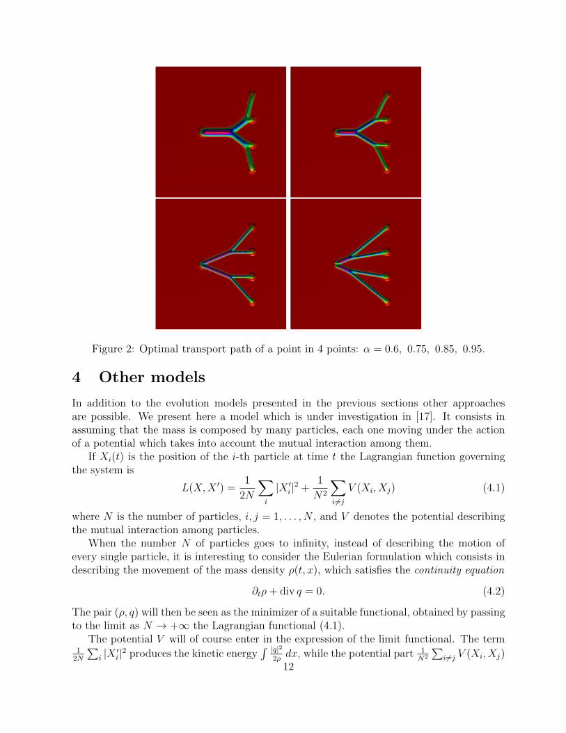
Figure 2: Optimal transport path of a point in 4 points: α = 0.6, 0.75, 0.85, 0.95.

4 Other models

In addition to the evolution models presented in the previous sections other approachesare possible. We present here a model which is under investigation in [17]. It consists inassuming that the mass is composed by many particles, each one moving under the actionof a potential which takes into account the mutual interaction among them.

If Xi(t) is the position of the i-th particle at time t the Lagrangian function governingthe system is

L(X,X ′) =1

2N

∑i

|X ′i|2 +1

N2

∑i 6=j

V (Xi, Xj) (4.1)

where N is the number of particles, i, j = 1, . . . , N , and V denotes the potential describingthe mutual interaction among particles.

When the number N of particles goes to infinity, instead of describing the motion ofevery single particle, it is interesting to consider the Eulerian formulation which consists indescribing the movement of the mass density ρ(t, x), which satisfies the continuity equation

∂tρ+ div q = 0. (4.2)

The pair (ρ, q) will then be seen as the minimizer of a suitable functional, obtained by passingto the limit as N → +∞ the Lagrangian functional (4.1).

The potential V will of course enter in the expression of the limit functional. The term1

2N

∑i |X ′i|2 produces the kinetic energy

∫ |q|22ρdx, while the potential part 1

N2

∑i 6=j V (Xi, Xj)

12

Figure 3: Optimal transport path of a point in a circle: α = 0.6, 0.75, 0.85, 0.95.

gives rise to the term∫∫V (x, y)ρ(x)ρ(y) dx dy. Summarizing, we end up with the energy

functional

E(ρ, q) =

∫ T

0

(∫ |q|22ρ

dx+

∫∫V (x, y)ρ(x)ρ(y) dx dy

)dt

that has to be minimized among all pairs (ρ, q) which satisfy the continuity equation (4.2)together with initial and final conditions ρ(0, ·) = ρ0 and ρ(1, ·) = ρ1.

The energy E(ρ, q) above has to be better detailed when ρ(t, ·) is a singular measure,situation that may happen with some potential V . In the singular case the expression ofE(ρ, q) becomes

E(ρ, q) =

∫ T

0

(1

2

∫ ∣∣∣dqdρ

∣∣∣2 dρ+

∫∫V (x, y)ρ(dx)ρ(dy)

)dt. (4.3)

Under some mild conditions on the potential V it is possible to obtain an existence resultfor an optimal path ρ(t, x). Its behaviour, in terms of congestion or concentration effects,heavily depends on the form of the potential V . Clearly, a potential of repulsive type willproduce a congestion effect, while a potential of attractive type will produce concentration.

Example 4.1. In the two-dimensional case assume that the initial and final configurationsare

ρ0 = δA, ρ1 =1

2δB +

1

2δC ,

13

where A = (0, 0), B = (1, 1), C = (1,−1). In the case of an attractive potential theevolution consists of the motion of two particles that travel together up to a certain pointand then move symmetrically to reach their final destinations, respectively the points B andC. If

(x(t), y(t)

)is the path of the upper particle, we have x(t) = t and y(t) minimizes the

functional ∫ 1

0

(|y′|2 + V (2y)

)dt.

Then y(t) = 0 for t ≤ t0, where

t0 = 1−∫ 1

0

(V (2y)

)−1/2dy,

whiley′′ = ∇V (2y) for t > t0.

In the case V (y) = C|y|α with α > 0 we have

t0 = 0 if α ≥ 2, t0 = 1− 2(2−α)/2

(2− α)√C

if α > 2.

If 0 < t0 < 1 we find

y(t) =1

2

(√C(2− α)(t− t0)

)2/(2−α)for t > t0.

Note that if α→ 0 we get

t0 ≈ 1− 1√C

y(t) ≈√C(t− t0) for t > t0

which shows the branching transportation behaviour.Here are the plots of the transportation paths in some cases.

0.2 0.4 0.6 0.8 1.0

0.2

0.4

0.6

0.8

1.0

0.2 0.4 0.6 0.8 1.0

0.2

0.4

0.6

0.8

1.0

0.2 0.4 0.6 0.8 1.0

0.2

0.4

0.6

0.8

1.0

Figure 4: (a) V (y) = |y|2. (b) V (y) = 8|y|. (c) V (y) = 4|y|0.1.

Acknowledgements. This work is part of the project 2008K7Z249 Trasporto ottimo di massa,disuguaglianze geometriche e funzionali e applicazioni financed by the Italian Ministry ofResearch.

14

References

[1] L. Ambrosio: Lecture notes on optimal transport problems. In “Mathematical aspectsof evolving interfaces”, Funchal 2000, Lect. Notes Math. 1812, Springer-Verlag, Berlin(2003).

[2] L. Ambrosio, N. Gigli, G. Savare: Gradient flows in metric spaces and in thespace of probability measure. Second edition. Lectures in Mathematics ETH Zurich,Birkhauser Verlag, Basel (2008).

[3] L. Ambrosio, P. Tilli: Topics on Analysis in Metric Spaces. Oxford Lecture Ser.Math. Appl. 25, Oxford University Press, Oxford (2004).

[4] L. Ambrosio, A. Pratelli: Existence and stability results in the L1 theory of optimaltransportation. In “Optimal transportation and applications”, Martina Franca 2001,Lect. Notes Math. 1813, Springer-Verlag, Berlin (2003), 123–160.

[5] J.D. Benamou, Y. Brenier: A computational fluid mechanics solution to the Monge–Kantorovich mass transfer problem. Numer. Math., 84 (2000), 375–393.

[6] G. Bouchitte, G. Buttazzo: New lower semicontinuity results for nonconvex func-tionals defined on measures. Nonlinear Anal., 15 (1990), 679–692.

[7] G. Bouchitte, G. Buttazzo: Integral representation of nonconvex functionals de-fined on measures. Ann. Inst. H. Poincare Anal. Non Lineaire, 9 (1992), 101–117.

[8] G. Bouchitte, G. Buttazzo: Relaxation for a class of nonconvex functionals definedon measures. Ann. Inst. H. Poincare Anal. Non Lineaire, 10 (1993), 345–361.

[9] A. Brancolini, G. Buttazzo, F. Santambrogio: Path functionals over Wasser-stein spaces. J. Eur. Math. Soc., 8 (2006), 415–434.

[10] L. Brasco: Curves of minimal action over metric spaces. Ann. Mat. Pura Appl., 189(2010), 95–125.

[11] L. Brasco: Geodesics and PDE methods in transport models. Ph.D. Thesis, Universitadi Pisa N Universite Paris-Dauphine (2010), available at http://cvgmt.sns.it/.

[12] L. Brasco, G. Buttazzo, F. Santambrogio: A Benamou-Brenier approach tobranched transport. SIAM J. Math. Anal., 43 (2) (2011), 1023–1040.

[13] L. Brasco, F. Santambrogio: An equivalent path functional formulation ofbranched transportation problems. Discrete Contin. Dyn. Syst., 29 (2011), 845–871.

[14] L. Brasco, G. Carlier, F. Santambrogio: Congested traffic dynamics, weak flowsand very degenerate elliptic equations. J. Math. Pures Appl., 93 (2010), 652–671.

[15] Y. Brenier: Extended Monge-Kantorovich theory. In “Optimal transportation andapplications”, Lect. Notes Math. 1813, Springer-Verlag, Berlin (2003), 92–121.

15

[16] G. Buttazzo, C. Jimenez, E. Oudet: An optimization problem for mass trans-portation with congested dynamics. SIAM J. Control Optim., 48 (2009), 1961–1976.

[17] G. Buttazzo, E. Oudet: Dynamic transport problems with particles interactionterms. Paper in preparation.

[18] L. Caffarelli, M. Feldman, R.J. McCann: Constructing optimal maps forMonge’s transport problem as a limit of strictly convex costs. J. Amer. Math. Soc.,15 (2002), 1–26.

[19] J. Dolbeault, B. Nazaret, G. Savare: A new class of transport distances betweenmeasures. Calc. Var. Partial Differential Equations, 34 (2009), 193–231.

[20] L.C. Evans, W. Gangbo: Differential equation methods for the Monge-Kantorovichmass transfer problem. Memoirs Amer. Math. Soc. 653, (1999).

[21] E.N. Gilbert: Minimum cost communication networks. Bell System Tech. J., 46(1967), 2209–2227.

[22] L.V. Kantorovich: On the transfer of masses. Dokl. Akad. Nauk. SSSR, 37 (1942),199–201. English translation in J. Math. Sci., 133, (2006), 1381–1382.

[23] B. Maury, A. Roudneff-Chupin, F. Santambrogio: A macroscopic crowd mo-tion model of the gradient-flow type. Math. Models Methods Appl. Sci., 20 (10) (2010),1787–1821.

[24] G. Monge: Memoire sur la theorie des deblais et des remblais. Histoire Acad. SciencesParis, (1781), 666–704.

[25] V.N. Sudakov: Geometric problems in the theory of infinite dimensional distributions.Proc. Steklov Inst. Math., 141 (1979), 1–178.

[26] N.S. Trudinger, X.J. Wang: On the Monge mass transfer problem. Calc. Var. PDE,13 (2001), 19–31.

[27] C. Villani: Topics in optimal transportation. Graduate Studies in Mathematics 58,American Mathematical Society, Providence (2003).

[28] C. Villani: Optimal transport, old and new. Grundlehren der Mathematischen Wis-senshaften 338, Springer-Verlag, Berlin (2009).

[29] Q. Xia: Optimal paths related to transport problems. Commun. Contemp. Math., 5(2003), 251–279.

16