evolution of phase strains during tensile loading of

CO

MM

UN

ICATIO

N
DOI: 10.1002/adem.201200204
Evolution of Phase Strains During Tensile Loading of BovineCortical Bone**

By Anjali Singhal,* Fang Yuan, Stuart R. Stock, Jonathan D. Almer,L. Catherine Brinson and David C. Dunand

Synchrotron X-ray scattering is used to measure average strains in the two main nanoscale phases ofcortical bone – hydroxyapatite (HAP) platelets and collagen fibrils – under tensile loading at bodytemperature (37 8C) and under completely hydrated conditions. Dog-bone shaped specimens from bovinefemoral cortical bone were prepared from three anatomical quadrants: anterio-medial, anterio-lateral, andposterio-lateral. The apparent HAP and fibrillar elastic moduli – ratios of tensile stress as applied externallyand phase strains as measured by diffraction – exhibit significant correlations with the (i) femur quadrantfrom which the samples are obtained, (ii) properties obtained at the micro-scale using micro-computedtomography, i.e., microstructure, porosity and attenuation coefficient, and (iii) properties at the macro-scaleusing thermo-gravimetry and tensile testing, i.e., volume fraction and Young’s modulus. Comparison ofthese tensile apparent moduli with compressive apparent moduli (previously published for samples from thesame animal and tested under the same temperature and irradiation conditions) indicates that collagendeforms plastically to a greater extent in tension. Greater strains in the collagen fibril and concomitantgreater load transfer to the HAP result in apparent moduli that are significantly lower in tension than incompression for both phases. However, tensile and compressive Young’s moduli measured macroscopicallyare not significantly different during uniaxial testing.

[*] Dr. A. Singhal, Dr. F. Yuan, Dr. L. C. Brinson, Dr. D. C. DunandDepartment of Materials Science and Engineering, North-western University, Evanston, IL 60208, USAE-mail: [email protected]

Dr. S. R. StockDepartment of Molecular Pharmacology and BiologicalChemistry, Feinberg School of Medicine, Northwestern Uni-versity, Chicago, IL 60611, USA

Dr. J. D. AlmerX-ray Sciences Division, Argonne National Laboratory,Argonne, IL 60438, USA

Dr. L. C. BrinsonDepartment of Mechanical Engineering, Northwestern University,Evanston, IL 60208, USA

[**] The authors thank Dr. Alix Deymier-Black (NU) for numeroususeful discussions throughout this work as well as assistancewith the diffraction experiments at the APS beamline 1-ID-C.They also acknowledge Dr. Xianghui Xiao (APS) for his helpwith the micro-CT experiments at APS beamline 2BM. Use ofthe Advanced Photon Source was supported by the U.S. Depart-ment of Energy, Office of Science, Office of Basic EnergySciences, under Contract No. DE-AC02-06CH11357.

238 wileyonlinelibrary.com � 2013 WILEY-VCH Verlag GmbH & Co

Bone is a hierarchical structural composite consisting

of a complex combination of calcium hydroxyapatite

[Ca3(PO4)10(OH)2), HAP], collagen and water, whose.[1,2]

Mammalian long bones are occasionally subjected to near

uniaxial tension, e.g., in primates displaying suspensory

behavior and, in particular, brachiation,[3] and in humans

during surgical procedures such as limb lengthening by the

Ilizarov technique.[4] The primary loading modes of long

bones are bending or compression;[5] for bending, depending

on the position of the neutral stress axis in the transverse-

section of the cortical bone and the curvature of the long

bone, regions can experience either a gradient of compressive

strains or a combination of tensile and compressive strains.[6]

Therefore, it is important to determine the properties of

cortical bone in both tension and compression, which in turn

can provide information about deformation in bending mode.

Bone forms and remodels in response to the loads experienced

in vivo,[1,7] making its properties heterogeneous and depen-

dent on the location. Thus, it is also important to perform

measurements on a population of samples in order to obtain

statistically significant and reproducible properties. Also, a

more complete understanding of the distribution of stresses

. KGaA, Weinheim ADVANCED ENGINEERING MATERIALS 2013, 15, No. 4

CO

MM

UN

ICATIO

N

A. Singhal et al./Evolution of Phase Strains During Tensile Loading

(dependent on the local stiffness which may be different in

tension and compression) in the femur will lead to improve-

ments in the design of novel implant materials.[8]

The strength of cortical bone is greater in compression

than in tension due to the different forms of microstructural

damage; compressive deformation involves shear-type

cracks at planes oblique to the direction of loading, while

tensile deformation involves cracks separating various

microstructural features, like osteons and lamellae, at their

boundaries.[9,10–12] Three-point bending tests on human

cortical bones have shown that, as the specimen is loaded,

the inelastic tensile strains become progressively higher than

the compressive strains.[10] Thus, it is clear that tensile failure

is the determining mode during failure in bending. Like many

anisotropic composite materials,[13] bone may also exhibit

differences between the elastic properties in the tensile and

compressive modes. Barak et al.[14] has shown using tests in

three-point bending on equine bones that the compressive

elastic modulus is significantly (p< 0.05) lower than the

tensile modulus by 6%. On the other hand, Reilly and

Burstein[11] found no difference between the elastic moduli in

human and bovine compact bone during uniaxial tensile and

compressive tests of 20 specimens. Riggs et al. testing equine

radii (26 specimens)[15] and Dempster and Liddicoat testing

human femora, tibiae, and humeri (21 specimens)[16] did not

find differences in the tensile and compressive moduli. One

challenge associated with these findings is that the species

to species variations in properties[12,17] further confounds the

true variation between tensile and compressive stiffness of

bone. Young’s modulus of bone depends on a number of other

factors such as fraction of secondary Haversian bone,[18]

mineral content,[19,20] density or porosity,[19,21] and orientation

of collagen fibers.[22] Yet another factor of considerable

importance is the testing environment since the hydration

state and temperature significantly affect the properties

under investigation.[23] None of the above studies used

body temperature during mechanical tests and only one

study (Barak et al.[14]) used completely hydrated conditions.

Evans[24] showed that drying increases the tensile modulus

of human cortical bone, and Bonfield and Li[25] showed that

bone’s elastic modulus decreases with increasing testing

temperature. It is thus important to determine the tensile

properties of bone, as close as possible, to physiological

conditions.

High-energy X-ray scattering is a technique which has been

in use to measure, in situ, the micromechanics of deformation

within the phases of metal matrix composites[26] and is

now being increasingly used to assess, in situ, the mechanical

response of mineralized biological materials such as bone,[27–34]

antler,[35] and tooth[36,37] during mechanical loading. The

technique offers a unique capability of measuring strains

within the nanoscopic phases of the materials while averaging

over the entire thickness of the sample, which can range from

a few millimeters to few centimeters. To date, the bulk of the

research has focused on compressive deformation and only a

few studies have investigated tensile deformation.[27,31,33]

ADVANCED ENGINEERING MATERIALS 2013, 15, No. 4 � 2013 WILEY-VCH Verl

Since biological samples show high spatial variability in

structure (and thus properties), it is important to understand

the extent of variability in the measured properties due to the

heterogeneity in the samples and to determine the repeatability

of the measurement technique. These points are addressed in

the present work by combining techniques spanning multiple

length scales. Tensile loading tests are performed at body

temperature (37 8C), in completely hydrated conditions, on

25 samples taken from different locations in the bovine femur

cross-section. The strains in the HAP phase and the fibrils,

averaged over a 3.6� 106 mm3 volume, are measured by a

combination of wide-angle (WAXS) and small-angle X-ray

scattering (SAXS). Macroscopic Young’s moduli of complete

samples are obtained through conventional tensile testing on

millimeter-sized dog-bone samples. The microstructure and

porosity of the samples are determined through micro-

Computed Tomography (micro-CT). Finally, the phase volume

fractions are determined through thermogravimetry. Finite-

element modeling is used to simulate the experimental

conditions and sample geometry to support the experimental

results. These results are compared with existing results from

compressive testing by Singhal et al.,[34] which were obtained

using the same technique and experimental setup on samples

taken from the same animal, in order to understand the

differences between the two types of loading with respect to

the structure of bone.

1. Materials and Methods

1.1. Sample Preparation

Bovine femurs of an 18-month old Black Angus cow were

obtained from a local slaughterhouse (Aurora Packing Company

Inc., Aurora, IL, USA) within an hour of slaughter. The bones

were cleaned of marrow and attached ligaments using scalpels.

Twenty five flat rectangular strips of cortical bone with

approximate dimensions 30� 10� 1.5 mm3 were cut from three

anatomical quadrants in a single cross-section of the femur, close

to the mid-diaphyseal region and with the 30 mm dimension

parallel to the long direction of the femur. The strips were then

mounted on a custom-built vertical and horizontal translational

stage, and a high-speed, low-torque abrasion aluminum oxide

tip (Dremel rotary tool, Multipro 395) was used to grind the

smallest faces into a dog-bone shape (Figure 1). The samples

have a central gage length of 5 mm, where the cross-section is

constant, and taper slightly over 2.5 mm before reaching a 5 mm

shoulder region with greater curvature and a 5 mm grip section.

The samples were hydrated with de-ionized water throughout

the preparation process. The dimensions of each sample were

measured using an optical microscope.

1.2. Scattering Measurements

All the samples were loaded in tension on an MTS-858

hydraulic loading frame, with clamping grips custom-made

for tensile testing of small samples. A hydration container

made of stiff polymer was attached to the grips, which

circulated body temperature (37 8C) phosphate buffered saline

ag GmbH & Co. KGaA, Weinheim http://www.aem-journal.com 239

CO

MM

UN

ICATIO

N


Fig. 1. Sample geometry (to scale). The lower half of the sample shows the scattering(black filled circles) and micro-CT (green box) measurement locations on the tensilesample. The top half of the sample shows a map of longitudinal stresses (expressed inGPa) for a gripping compressive stress of 30 MPa over the gripping section shown bythe red box, and an applied tensile load of 183 N (corresponding to 61 MPa in the gagesection). The blue box corresponds to the gage section. Scattering measurements arecarried out on the lower half of the sample. The measurement locations are overlaidon the stress distribution map in the top half for illustration purpose, given that thesample is symmetrical.

(PBS) around the samples throughout testing. The samples

were loaded in steps of 21 N up to a maximal load of 180 N,

and unloaded to 0 N in a single step. For each increment of

load, WAXS and SAXS patterns (see below) were recorded at

five different locations. Due to limited vertical translation

range, the lowermost measurement on the sample (Location 1)

was in the shoulder region, about 1.5 mm from the top of the

lower grip (red box in Figure 1). Measurements were done at a

spacing of 1 mm in the vertical direction, as indicated in the

bottom half of the sample in Figure 1: Location 5 was thus in

the region with a slight taper. The locations marked on the

top half of the sample are for illustration purpose, given

that the sample is symmetrical. The sample was horizontally

centered with respect to the X-ray beam using absorption

measurements.

Scattering measurements were performed at station 1-ID-C

at APS at two different length scales: WAXS (A-level

240 http://www.aem-journal.com � 2013 WILEY-VCH Verlag GmbH & C

periodicities) and SAXS (nm-level periodicities). The WAXS

rings are from Bragg diffraction from regularly arranged

atoms in each of the array of HAP crystals, whereas the

SAXS rings originate from scattering due to electron density

differences between the periodically arranged HAP crystals

and the collagen matrix framework.[28] The setup for

mechanical testing and scattering measurements is similar

to previous works.[30,32] The WAXS patterns were recorded

by a GE-41RT flat-panel detector (2048� 2048 pixels,

200 mm2 pixel�1), placed 1118 mm from the sample, while

the SAXS patterns were recorded by a PI-CCD detector

(1152� 1242 pixels, 22.5 mm pixel�1) placed 4000 mm from the

sample. X-ray with a beam size of 50� 50 mm2 and 70 keV

energy was used for the measurements. The X-ray exposure

was 1 s for a single WAXS or SAXS measurement, resulting

in a dose of 0.6 kGy for a combined WAXS and SAXS

measurement (see Appendix for calculation). These X-ray

exposure times were as short as possible in order to keep

irradiation damage below threshold levels as determined in

our previous work.[30,33]

1.3. Young’s Modulus Measurements

Young’s moduli of the samples were determined in a

separate experiment after the scattering measurements on

four samples from the anterio-medial, five from the anterio-

lateral, and five from the posterio-lateral quadrants. Strain

gages were attached to each of these samples to measure

longitudinal strains. The samples were loaded to 60 MPa in

100 s at ambient temperature. This rate of loading is higher

than the quasi-static loading carried out during in situ

diffraction and mechanical testing, where the samples were

held at each load for 246 s to allow time for the diffraction

measurements at five different locations on each sample. Also,

the samples were not kept hydrated during these macroscopic

measurements so as to keep the strain gage adhered to the

bone surface during testing. This resulted in the drying of the

samples as the experiment proceeded. The total duration of

the macroscopic modulus measurements was about 10–15 min

which included loading of the samples, and measurement.

However, according to the work of Sedlin,[24] on bending

properties of human cortical bone, the elastic modulus did not

change significantly for air drying up to 60 min. Thus the

duration for which the samples underwent drying is not

expected to significantly affect the measured modulus. Also,

since the gage section of the each sample was hand-machined,

any non-uniformity in the cross-section of the gage region of

the sample will be propagated, resulting in the variation of

the measured modulus from its actual value (in the case of a

perfectly uniform cross-section).

An aluminum (2024-T3 alloy) standard sample, of the same

shape and size as the bone samples, was tested first using a

strain gage which measured longitudinal strains. The

standard sample was loaded up to 75 MPa in load-control,

in 100, 200, or 1000 s. The resulting Young’s moduli values did

not depend on loading rate and averaged 81.9� 0.9 GPa, about

12% higher than the literature value of 73.1 GPa.[38] The bone

o. KGaA, Weinheim ADVANCED ENGINEERING MATERIALS 2013, 15, No. 4

CO

MM

UN

ICATIO

N


Young’s modulus reported in Section 3.2 is corrected by this

percentage difference.

1.4. Absorption Measurements Using Micro-ComputedTomography

Synchrotron micro-CT was performed on the bone samples

at station 2-BM at APS. Due to beam-time limitations, 5 of

25 samples could not be imaged. The bone samples were

air-dried overnight after mechanical testing to reduce motion

artifacts due to drying. The samples were imaged with

20.7 keV X-rays and reconstructed with 2.9 mm isotropic

volume elements (voxels). A total of 1024 (2K)2 slices were

recorded and covered 2.9 mm of the sample length (green

rectangular box in Figure 1) and one of the positions where

the scattering measurements were previously performed

(Location 5 in Figure 1).

The reconstructed 2D slices were visualized using ImageJ.

Each reconstructed slice is a map of the linear attenuation

coefficient. For each specimen, the mean linear attenuation

coefficient was calculated for each of six slices spaced 0.29 mm

apart. The mean for each sample was the average of the slice

average values. The slices near the top and bottom of the

imaged volume were not included in this analysis because of

low contrast.

Porosity was quantified in the same six slices of each

sample. The area fraction of voids was calculated for the entire

bone cross-section of each slice using the same segmentation

threshold. Each specimen’s porosity was the average of its

six slices. The microstructure of the sample was determined

from the reconstructed image slices. All the samples

examined either had a plexiform or a Haversian microstruc-

ture corresponding to a microstructure index of zero or one,

respectively.

1.5. Thermogravimetric Measurements

Thermogravimetric analysis (TGA) was performed on all

25 samples to determine the volume fractions of the three

phases – HAP, collagen, and water – in bone. This was

performed using a Mettler-Toledo instrument calibrated with

pure In and Al standards. TGA samples, weighing approxi-

mately 3–10 mg, were cut from the bone samples after

mechanical testing, close to Location 5 sampled by the

X-ray beam (Figure 1). They were heated from 25 to 680 8C at a

rate of 10 8C min�1 in air following earlier TGA procedures

for bone.[34,39] As in these studies, the TGA mass loss curves

exhibit three distinct regions. The difference in the mass of

the sample between two transition temperatures (25, 205,

and 545 8C) gives the weight fractions of water, collagen and

HAP. These weight fractions are then converted into volume

fractions using densities of 1.0 g cm�3 for water, 1.1 g cm�3 for

collagen, and 3.2 g cm�3 for HAP.[1]

1.6. Scattering Analysis

The X-ray scattering data analysis has been described in our

previous studies and will be summarized here briefly.[28,30]

The WAXS diffraction patterns are calibrated using a pressed


ceria powder disk. The radial center of the 00.2 peak is

determined at each azimuthal angle. The longitudinal HAP

strains are determined using the radii at azimuths of 908� 108and 2708� 108.[28] The analysis of the SAXS data proceeds in a

similar way by determining the radial center of the third order

D-period peak at approximately 67/3¼ 22.3 nm. The long-

itudinal strains at a particular stress are calculated by taking

an average over �158 about the maximum peak intensity at

908 and 2708 azimuths. The WAXS and SAXS strains are

reported as a function of stress; the slope of this plot is

calculated by taking a linear best-fit and termed as the HAP

and fibrillar apparent modulus, respectively.[30] Data points

which deviated grossly from linearity, either at the highest

or lowest stresses, were not used for this best-fit slope

determination. In all these cases, at least five data points were

used for least-squares slope determination.

The azimuthal angle of the maximum intensity of the

00.2 diffraction ring was quantified for all positions on all

specimens before loading. The azimuthal full-width at

half-maximum intensity (h-FWHM) was also measured for

each ring maxima.

1.7. Statistical Analysis

Significant differences in the means of the HAP and fibrillar

apparent moduli for different populations were accepted at

a significance level of p< 0.05 by the one-way ANOVA

(Analysis Of Variance) method, using OriginPro 8.6 (Origin

Lab, Northampton, MA, USA). In cases where significant

differences were measured, pair-wise t-tests were used to

determine which of the population means differed, also at

p< 0.05.

In Table 1, when continuously varying data was compared

with categorical data, i.e., microstructure index (two cate-

gories), the former was separated into the two categories,

and significant differences and correlation coefficients were

determined using ANOVA.

1.8. Finite Element Modeling

The non-uniform cross-sections at Locations 1–5 in the

dog-bone shaped samples result in non-uniform distribution

of stress. Finite element analysis was used to determine the

distribution of stresses within the samples. The longitudinal

stresses were averaged in the direction of travel of the X-ray

beam through the sample, i.e., along the 1.5 mm thickness

direction, to obtain the average longitudinal stresses at

different measurement locations.

The finite element simulation was implemented using

ABAQUS 6.10-EF1. The geometry in the model reproduced

the dimensions of the dog-bone shaped samples used for the

experiments (see Figure 1): 5.0 mm� 5.0 mm for the gripping

region, 2.0 mm width� 5.0 mm length for the central gage

region; the two 7.5-mm long shoulder regions between the

gripping and gage regions were connected by smooth curves.

The curves were obtained by connecting the width values

determined through the optical microscope at the locations at

which X-ray scattering measurements were done (3.96 mm


CO

MM

UN

ICATIO

N


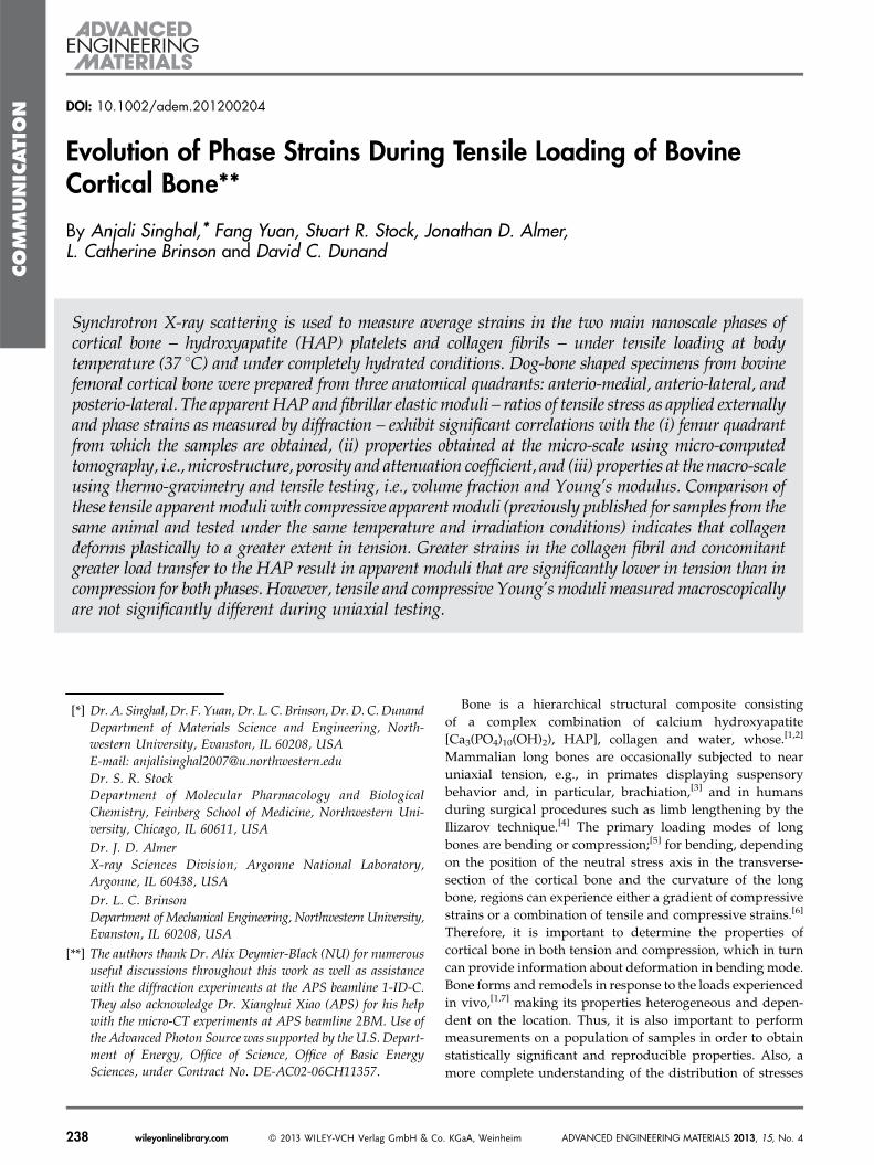
Table 1. Pearson’s correlation coefficients for HAP, fibrillar, and Young’s moduli, attenuation coefficient (m), porosity, microstructure index, and HAP volume fraction in thesamples. The microstructure index takes a value of zero or unity, respectively, for plexiform or Haversian microstructure.

R HAPmodulus

Fibrillarmodulus

Macroscopicmodulus

Attenuationcoefficient

HAPfraction

Porosityfraction

Fibrillar modulus 0.42

Macroscopic modulus 0.31 0.17

Attenuation coefficient 0.14 �0.11 0.55HAP fraction 0.20 �0.04 0.66 0.90

Porosity fraction �0.30 �0.27 �0.51 �0.55 �0.72

Microstructure �0.50 �0.10 �0.67 �0.69 �0.73 0.67

The values indicated in bold are significant at p< 0.05, those in italics are significant at p< 0.3, and the rest are all p> 0.3.

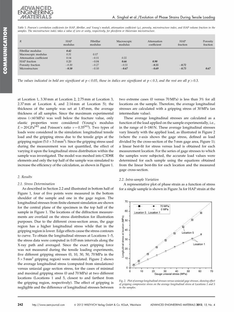
Fig. 2. Plot of average longitudinal stresses versus uniaxial gage stresses, showing effectof gripping compressive stress on the average longitudinal stress at Locations 1 and 5in the samples.

at Location 1, 3.30 mm at Location 2, 2.75 mm at Location 3,

2.37 mm at Location 4, and 2.14 mm at Location 5); the

thickness of the sample was set at 1.45 mm, the average

thickness of all samples. Since the maximum experimental

stress (<60 MPa) was well below the fracture value, only

elastic properties were considered (Young’s modulus

E¼ 20 GPa[40] and Poisson’s ratio n¼ 0.35[41]). Two types of

loads were considered in the simulation: longitudinal tensile

load and the gripping stress due to the tensile grips at the

gripping region (5.0� 5.0 mm2). Since the gripping stress used

during the measurement was not quantified, the effect of

varying it upon the longitudinal stress distribution within the

sample was investigated. The model was meshed into C3D8R

elements and only the top half of the sample was simulated to

increase the efficiency of the calculation, as shown in Figure 1.

2. Results

2.1. Stress Determination

As described in Section 2.2 and illustrated in bottom half of

Figure 1, four of five points were measured in the bottom

shoulder of the sample and one in the gage region. The

longitudinal stresses from finite element simulation are shown

for the central plane of the specimen in the top half of the

sample in Figure 1. The locations of the diffraction measure-

ments are overlaid on the stress distribution for illustration

purposes. Due to the different cross-section areas, the gage

region has a higher longitudinal stress while that in the

gripping region is lower. Edge effects cause the stress contours

to curve. To obtain the longitudinal stresses at Locations 1–5,

the stress data were computed in 0.05 mm intervals along the

X-ray path and averaged. Since the exact gripping force

was not measured during the tensile loading experiments,

five different gripping stresses (0, 10, 30, 50, 70 MPa in the

5� 5 mm2 gripping region) were simulated. Figure 2 shows

the average longitudinal stress (computed from simulations)

versus uniaxial gage section stress, for the cases of minimal

and maximal gripping stress (0 and 70 MPa) at two different

locations (Locations 1 and 5, closest to and farthest from

the gripping region, respectively). The effect of gripping is

negligible and the difference of longitudinal stresses between


two extreme cases (0 versus 70 MPa) is less than 3% for all

locations on the sample. Therefore, the average longitudinal

stresses are calculated with a gripping stress of 30 MPa (an

intermediate value).

These average longitudinal stresses are calculated as a

function of the load applied on the sample experimentally, i.e.,

in the range of 0–180 N. These average longitudinal stresses

vary linearly with the applied load, as illustrated in Figure 2

(where the x-axis shows the gage stress, defined as load

divided by the cross-section of the 5 mm gage area, Figure 1);

a linear best-fit for stress versus load is obtained for each

measurement location. For the series of gage stresses to which

the samples were subjected, the accurate load values were

determined for each sample using the equations obtained

from the linear best-fits for each location and the measured

gage cross-section.

2.2. Intra-sample Variation

A representative plot of phase strain as a function of stress

for a single sample is shown in Figure 3a for HAP strain at the


CO

MM

UN

ICATIO

N


five locations, and in Figure 3b for fibrillar strain at four

locations. The fibrillar strains at Location 4 in this sample were

very scattered and hence not shown here. For this sample,

EappHAP is 19.2� 2.9 GPa and E

appFib is 3.0� 1.4 GPa, as averaged

over the five locations (four locations for fibrillar modulus).

Figure 3c shows a box plot of the apparent HAP moduli (EappHAP)

measured over all 25 samples and at all five locations in each

sample, corresponding to 125 data points. In the case of

fibrillar moduli, sample AL8 had very weak scattered

intensity from all five locations in the SAXS, and the peak-fits

were very poor; this sample was eliminated from EappFib

averages. Additionally, 19 other EappFib values were eliminated

(6 from Location 1, 3 from Location 2, 2 from Location 3, 6 from

Location 4, and 2 from Location 5) because the fitted strain

values were very scattered from one stress to another.

Fig. 3. Plots of longitudinal stress versus (a) HAP strain for all five locations in sample AMHAP and fibrillar modulus at each location. Crosses indicate the data points not used for slopfor each box) (d) Box plot for apparent fibrillar modulus (n¼ 18, 21, 22, 18, and 22 in order omean, (~!) are the maximum and minimum values. The whiskers extend out to the 95


Figure 3d thus shows a box plot for a total of 101 EappFib from

24 samples. Statistical analysis (Section 2.7) was performed

on EappHAP values grouped according to their five positions, in

all samples. At Location 5, EappHAP is significantly greater than

at Locations 1, 2, and 3 (p< 0.05); EappHAP at Location 4 is

significantly greater than at Location 1; EappHAP at Location 2 is

significantly greater than at Location 1. The fibrillar moduli

(EappFib ) do not differ significantly between the five locations.

The average intra-sample standard deviation for apparent

elastic modulus across the five locations in each sample is

4.1 GPa for HAP and 1.6 GPa for the fibrils. Because system-

atically increasing or decreasing trends with position are not

found in the HAP or fibrillar apparent moduli, the mean of

these five measurement locations hereafter are used when

comparing specimens.

5. (b) Fibrillar strain for four locations in sample AM5. Best fit line gives the apparente determination. (c) Box plot showing the distribution of apparent HAP modulus (n¼ 25f Locations 1–5). The solid line within the box is the median of the distribution, (&) is theth and 5th percentiles, and the box represents the 75th, 50th, and 25th percentiles.


CO

MM

UN

ICATIO

N


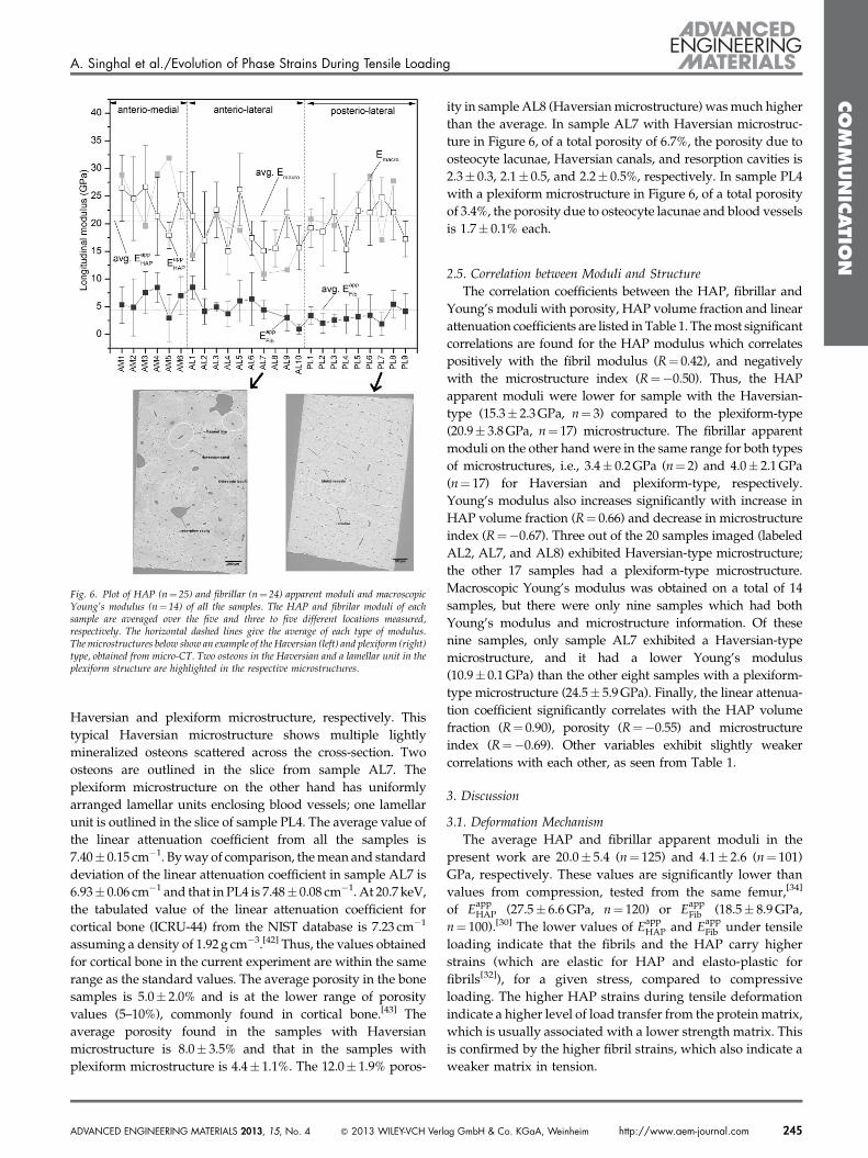
Fig. 5. Box plot of the quadrant-wise comparison of the HAP (n¼ 30, 50, and 45 left toright) and fibrillar (n¼ 28, 40, and 33 left to right) apparent moduli for all the samples.Signification of boxes, symbols and lines are as in Figure 3b and c.

2.3. Moduli and Anatomical Position

The apparent HAP moduli were first grouped according to

their position in the femur cross-section: anterior (which

includes anterio-medial and anterio-lateral quadrants) or

posterior (which has only the posterio-lateral quadrant).

Figure 4 shows a box plot of the HAP and fibrillar moduli

which includes all five locations (three to five locations for

fibrils) measured in each sample. No statistically significant

difference exists between EappHAP of the anterior (19.7� 6.0 GPa,

n¼ 80) and posterior (20.4� 4.4, n¼ 45) sides. The fibrillar

apparent moduli, on the other hand, are significantly higher at

the anterior side (4.7� 2.8 GPa, n¼ 67) than the posterior side

(2.9� 1.8 GPa, n¼ 33) as seen in Figure 4.

The moduli were then grouped according to their

quadrants, i.e., anterio-medial, anterio-lateral, and poster-

io-lateral. As seen in Figure 5, the HAP apparent moduli in the

anterio-lateral quadrant (17.4� 4.1 GPa, n¼ 50) are signifi-

cantly lower than those in the anterio-medial (23.6� 6.6 GPa,

n¼ 30) ( p< 0.001) and the posterio-lateral quadrant

(20.4� 4.4 GPa, n¼ 45) (p¼ 0.001). Also, the HAP apparent

moduli in the anterio-medial quadrant are significantly

greater than the posterior-lateral quadrant (p¼ 0.013). A

quadrant-wise comparison of the fibrillar apparent moduli

also showed (Figure 5) that the values in the anterio-medial

quadrant (5.8� 3.0 GPa, n¼ 28) were significantly greater than

the anterio-lateral (3.9� 2.3 GPa, n¼ 39) (p¼ 0.006) and the

posterior-lateral (2.9� 1.9 GPa, n¼ 33) quadrants (p< 0.001).

The fibrillar apparent moduli in the anterio-lateral quadrant

are significantly greater than in the posterior-lateral quadrant

(p¼ 0.036). The average macroscopic Young’s modulus

(Emacro) in the anterio-medial quadrant (31.1� 6.0 GPa,

n¼ 4) is also greater than the anterio-lateral quadrant

(17.5� 5.2 GPa, n¼ 5) (p¼ 0.009), and the anterio-lateral

quadrant is lower than the posterior-lateral quadrant

(25.9� 5.8 GPa, n¼ 5) ( p¼ 0.044). A similar grouping was

done with the corresponding h-FWHM of the samples to

Fig. 4. Box plot of the HAP (n¼ 80 and 45 left to right) and fibrillar (n¼ 68 and 33 leftto right) apparent modulus for anterior and posterior samples. Signification of boxes,symbols, and lines are as in Figure 3b and c.


determine any significant differences between the quadrants.

The anterio-medial quadrant had significantly lower

h-FWHM values (538� 48) than the anterio-lateral (578� 68)(p¼ 0.003) and the posterio-lateral (618� 88) quadrants

(p< 0.001). One single sample (AL8) had a h-FWHM value

of 1128� 238. The maximum intensity azimuthal angle is

found to vary from 708 to 1208 in most samples and was 1408 in

one single case (AL8), indicating that the (00.l) peak was not

perfectly aligned with the loading/longitudinal direction.

Figure 6 shows the HAP and fibrillar apparent moduli,

EappHAP and E

appFib , and the Emacro for the different samples

measured. By averaging the slopes from all of the five

locations for HAP, and three to five locations for fibrils, from

all of the 25 samples for HAP (125 slopes), and 24 samples for

fibrils (101 slopes), the overall HAP and fibrillar moduli were

calculated to be 20.0� 5.4 and 4.1� 2.6 GPa, respectively

(dotted lines in Figure 6). The average value of the Emacro

obtained over 14 samples is 21.5� 6.8 GPa (dotted line in

Figure 6). The large spread in the apparent moduli values

reflects positional variations within individual samples.

The inter-sample standard deviations calculated between

the average apparent elastic moduli measured for each

sample are 3.7 GPa for HAP, and 2.1 GPa for the fibrils. These

inter-sample variations are similar to the observed intra-

sample variations of 4.1 and 1.6 GPa for HAP and fibrils,

respectively (Section 3.2). It is apparent that the mean

macroscopic Young’s modulus is lower in the anterio-lateral

quadrant compared to the anterio-medial and posterior-

lateral quadrants. This trend is also exhibited by both the HAP

and fibrillar apparent moduli.

2.4. Microstructure

The reconstructed slices in Figure 6 show representative

microstructures from two samples, AL7 and PL4, which have a


CO

MM

UN

ICATIO

N


Fig. 6. Plot of HAP (n¼ 25) and fibrillar (n¼ 24) apparent moduli and macroscopicYoung’s modulus (n¼ 14) of all the samples. The HAP and fibrilar moduli of eachsample are averaged over the five and three to five different locations measured,respectively. The horizontal dashed lines give the average of each type of modulus.The microstructures below show an example of the Haversian (left) and plexiform (right)type, obtained from micro-CT. Two osteons in the Haversian and a lamellar unit in theplexiform structure are highlighted in the respective microstructures.

Haversian and plexiform microstructure, respectively. This

typical Haversian microstructure shows multiple lightly

mineralized osteons scattered across the cross-section. Two

osteons are outlined in the slice from sample AL7. The

plexiform microstructure on the other hand has uniformly

arranged lamellar units enclosing blood vessels; one lamellar

unit is outlined in the slice of sample PL4. The average value of

the linear attenuation coefficient from all the samples is

7.40� 0.15 cm�1. By way of comparison, the mean and standard

deviation of the linear attenuation coefficient in sample AL7 is

6.93� 0.06 cm�1 and that in PL4 is 7.48� 0.08 cm�1. At 20.7 keV,

the tabulated value of the linear attenuation coefficient for

cortical bone (ICRU-44) from the NIST database is 7.23 cm�1

assuming a density of 1.92 g cm�3.[42] Thus, the values obtained

for cortical bone in the current experiment are within the same

range as the standard values. The average porosity in the bone

samples is 5.0� 2.0% and is at the lower range of porosity

values (5–10%), commonly found in cortical bone.[43] The

average porosity found in the samples with Haversian

microstructure is 8.0� 3.5% and that in the samples with

plexiform microstructure is 4.4� 1.1%. The 12.0� 1.9% poros-


ity in sample AL8 (Haversian microstructure) was much higher

than the average. In sample AL7 with Haversian microstruc-

ture in Figure 6, of a total porosity of 6.7%, the porosity due to

osteocyte lacunae, Haversian canals, and resorption cavities is

2.3� 0.3, 2.1� 0.5, and 2.2� 0.5%, respectively. In sample PL4

with a plexiform microstructure in Figure 6, of a total porosity

of 3.4%, the porosity due to osteocyte lacunae and blood vessels

is 1.7� 0.1% each.

2.5. Correlation between Moduli and Structure

The correlation coefficients between the HAP, fibrillar and

Young’s moduli with porosity, HAP volume fraction and linear

attenuation coefficients are listed in Table 1. The most significant

correlations are found for the HAP modulus which correlates

positively with the fibril modulus (R¼ 0.42), and negatively

with the microstructure index (R¼�0.50). Thus, the HAP

apparent moduli were lower for sample with the Haversian-

type (15.3� 2.3 GPa, n¼ 3) compared to the plexiform-type

(20.9� 3.8 GPa, n¼ 17) microstructure. The fibrillar apparent

moduli on the other hand were in the same range for both types

of microstructures, i.e., 3.4� 0.2 GPa (n¼ 2) and 4.0� 2.1 GPa

(n¼ 17) for Haversian and plexiform-type, respectively.

Young’s modulus also increases significantly with increase in

HAP volume fraction (R¼ 0.66) and decrease in microstructure

index (R¼�0.67). Three out of the 20 samples imaged (labeled

AL2, AL7, and AL8) exhibited Haversian-type microstructure;

the other 17 samples had a plexiform-type microstructure.

Macroscopic Young’s modulus was obtained on a total of 14

samples, but there were only nine samples which had both

Young’s modulus and microstructure information. Of these

nine samples, only sample AL7 exhibited a Haversian-type

microstructure, and it had a lower Young’s modulus

(10.9� 0.1 GPa) than the other eight samples with a plexiform-

type microstructure (24.5� 5.9 GPa). Finally, the linear attenua-

tion coefficient significantly correlates with the HAP volume

fraction (R¼ 0.90), porosity (R¼�0.55) and microstructure

index (R¼�0.69). Other variables exhibit slightly weaker

correlations with each other, as seen from Table 1.

3. Discussion

3.1. Deformation Mechanism

The average HAP and fibrillar apparent moduli in the

present work are 20.0� 5.4 (n¼ 125) and 4.1� 2.6 (n¼ 101)

GPa, respectively. These values are significantly lower than

values from compression, tested from the same femur,[34]

of EappHAP (27.5� 6.6 GPa, n¼ 120) or E

appFib (18.5� 8.9 GPa,

n¼ 100).[30] The lower values of EappHAP and E

appFib under tensile

loading indicate that the fibrils and the HAP carry higher

strains (which are elastic for HAP and elasto-plastic for

fibrils[32]), for a given stress, compared to compressive

loading. The higher HAP strains during tensile deformation

indicate a higher level of load transfer from the protein matrix,

which is usually associated with a lower strength matrix. This

is confirmed by the higher fibril strains, which also indicate a

weaker matrix in tension.


CO

MM

UN

ICATIO

N


The average macroscopic Young’s modulus in the present

study is 21.5� 6.8 GPa (n¼ 14) which is within the broad

range of values, 18–32 GPa, found in literature for cortical

bones of species such as bovine, equine, human, deer, etc.,

loaded in tension.[12,44] The tensile average Young’s modulus

found in the present study is not significantly different

(p< 0.05) from the compressive value of 20.5� 1.5 GPa

(n¼ 23) found in our previous study on samples taken from

the same animal.[34] As discussed in Section 1, there is no

general agreement in the literature about the association

between the macroscopic tensile and compressive modulus.

Also, the compressive Young’s modulus is measured using

the ultrasonic speed-of-sound technique. Grimal et al.[45] have

reported that the ultrasonic modulus of cortical bone is about

21% higher than the modulus determined from mechanical

testing (three-point bend tests) due to stress-relaxation effects.

Thus, the difference between the compressive (20.5� 1.5 GPa)

and tensile Young’s modulus (21.5� 6.8 GPa) in the present

case could also result from the experimental variations

between the two techniques.

The flat dog-bone-shaped specimens in the present

experiment were loaded to the maximum 180 N (equivalent

approximately to a longitudinal stress of 60 MPa at Location

5), thus resulting in a maximum macroscopic strain of about

0.060/21.5¼ 0.0028 (0.28%). In recent work by Hoo et al. on

bovine femoral bone,[27] it was shown that a sudden decrease

in the longitudinal HAP and fibrillar strains occurs beyond a

macroscopic tensile strain of 0.2%, and this was hypothesized

to occur due to localized plastic deformation; the macroscopic

stress–strain curve did not show any deviation from linearity

at this point. It was theorized that stress is redistributed from

longitudinally oriented and load-bearing mineralized col-

lagen fibrils to the laterally oriented nanoscale structures,

without affecting the total strain carried by the material.[27]

Similarly, we hypothesize here that localized plastic deforma-

tion takes place at the molecular collagen level which results in

large strains measured within the fibrils. The increased plastic

deformation within the collagen matrix results in a decrease

in the EappFib . The HAP/collagen interface is expected to be

minimally damaged due to irradiation because of the low

exposure times used to acquire X-ray scattering data.[30] There

could be loss of some van der Waals or hydrogen bonds at the

interface due to mechanical loading which would weaken

the interface,[30] thus decreasing load transfer from collagen to

HAP to some extent. However, the observed increase in load

transfer, and hence strain, to the reinforcement (HAP) results

in lower values of apparent moduli compared to compression

experiments.

The greater strain which is carried under tensile loading

by both phases also suggests that the collagen phase (being

more compliant than HAP) yields at lower stresses than under

compressive loading. The ratio of fibril to mineral strain in the

present work is calculated as 4:1, and is about 1.6–3.5 times

higher than the value of 5:2, for tensile testing on fibrolamellar

packets of bovine femoral bone, found by Gupta et al.,[31] and

8:7 for tensile testing on fibrolamellar bovine femoral bones,


found by Hoo et al.[27] The difference in the ratios can be

attributed to the different testing conditions [dried[27] versus

hydrated (present case)] and the influence of the structures

present at larger length scales, e.g., osteons, due to large

(millimeter-sized) samples being studied in the present case

compared to thin lamellar (50–100 mm thick) sections of bone

studied in ref.[31]. Our previous work on compressive loading

of bovine bone samples, which were taken from the same

animal as the samples in the present work, results in a fibril to

mineral strain ratio of 8:5.[34] This further confirms that the

fibrils deform to a much larger extent under tensile loading.

Furthermore, the fact that moduli in the present work are

being compared between samples taken from the same

animal, makes a strong case for the above finding, rather than

two studies on two different animals.

The mechanical properties of collagen obtained from a

variety of species, demineralized bone, and in vitro self-

assembled fibrils have been extensively characterized. The

extraction of individual collagen fibrils in their native state

poses a major challenge to the determination of its properties.

The most commonly found values for the Young’s modulus

of collagen range from 2 to 11 GPa when tested in ambient

conditions,[46] and 0.2–0.8 GPa under hydrated condi-

tions.[47,48] Whereas a lot of research has been performed on

collagen under tensile loading, almost no information exists

on its properties under compression. It is difficult to test

collagen under compressive loading due to its lack of rigidity

in the longitudinal direction.[47] However, it is reasonable to

assume that the behavior of collagen is different under tensile

and compressive loading because of its highly fibrous

structure which influences the overall load transfer behavior.

According to the studies of Dempster and Liddicoat on human

femurs,[16] plastic deformation of bone begins at about 36 MPa

in tension and 70 MPa in compression. Greater strains and

thus greater plastic deformation are then expected for collagen

fibrils loaded in tension. Moreover, since cortical bone is

predominantly loaded in compression or bending under

natural physiological circumstances, it has evolved to resist

compressive loads more effectively than tensile loads.[1,2]

3.2. Spatial Variations between Femur Quadrants

A comparison of Young’s moduli of samples taken from

three quadrants of the femur (Figure 6) shows that the

anterio-lateral region is significantly less stiff, in macroscopic

tension, compared with the anterio-medial and posterior-

lateral regions. This trend is also exhibited by the statistically

significant lower EappHAP in the anterio-lateral quadrant. This

suggests that the Young’s modulus and EappHAP depends on

similar factors as discussed in the following. The larger

variation in EappFib (Figure 6b), on the other hand, obscure any

trend. The lower azimuthal spread (FWHM) in the HAP 00.2

diffraction ring, and hence the orientation distribution of HAP

c-axes with respect to the longitudinal/loading direction,

in the anterio-medial region, compared to the anterio- and

posterior-lateral regions, is consistent with the lower EappHAP in

the latter two regions. The anisotropic elastic constants of


CO

MM

UN

ICATIO

N


HAP have been reported as C11¼ 137 GPa and C33¼ 172 GPa

in Katz and Ukrainci,[49] with the c-axis aligned along the 33

direction, which makes it the most load bearing direction.

Thus when there are fewer HAP platelets with c-axes aligned

with the longitudinal (or loading) direction in the sampled

volume, as in the anterio- and posterior-lateral quadrants,

the average strain on those HAP platelets increases, thus

decreasing the measured EappHAP.

The HAP, fibrillar, and Young’s moduli exhibit significant

correlations with the microstructure, porosity, HAP volume

fraction and the mean attenuation coefficient (Table 1).

The Young’s modulus of the sample increases with the

HAP content (R¼ 0.66), which is a good predictor of

bone stiffness.[19,20] This is similar to the behavior of a

short-fiber reinforced composite, where an increase in the

stiffer reinforcement content (HAP in this case) results in an

increase in the overall stiffness of the sample. As expected,

the linear attenuation coefficient, which reflects the mineral

content of specimen, also correlates with HAP volume fraction

(R¼ 0.90). Thus, linear attenuation coefficient also increases

the Young’s modulus (R¼ 0.55). The HAP apparent modulus

concomitantly increases with the Young’s modulus (R¼ 0.31),

but correlates much less significantly with the HAP fraction

(R¼ 0.20). For the latter correlation, as the fraction of stiff

HAP platelets increases, the average stress on each HAP

platelet decreases, resulting in an increase in the HAP

apparent modulus (¼sapplied/ephase). However, as compared

to the Young’s modulus, EappHAP increases less significantly

with HAP fraction (R¼ 0.2 versus 0.66). This may be because

the samples used to determine the HAP fraction are obtained

approximately from the region sampled by the X-ray beam,

and that region might not be completely representative

of the local volume fractions everywhere in the bulk

sample.[34] Also, an increase in the HAP apparent modulus

is accompanied by an increase in the fibrillar apparent

modulus (R¼ 0.42). The HAP modulus reflects the ability of

the HAP phase to bear load; the fibrillar modulus applies

to an HAP/collagen nano-composite, and reflects the

cooperative deformation between HAP and collagen. Greater

load carrying capacity of the HAP phase thus increases

the load carrying capacity of the whole fibril due to factors

discussed above. Thus, the correlation between fibrillar

modulus and HAP modulus is expected.

The distribution of microstructures in the transverse

cross-section of the femur used in the present experiment is

such that specimens of plexiform structure are found in most

of the anterio-medial, anterio-lateral, and posterior-lateral

regions. Specimens of Haversian structure are found in the

anterior and lateral ends of the femur cross-section. These

results are consistent with that of ref.[50], which reported a

similar relation between the spatial location and bone

microstructure. The correlation of microstructure with sample

porosity (R¼ 0.67) indicates that Haversian bone has greater

porosity than plexiform bone (8.0 versus 4.4% volume

fractions, respectively), which makes Haversian bone less

stiff both macroscopically (R¼�0.67) and at the nanoscale


level (EappHAP, R¼�0.50). Haversian bone is also less miner-

alized compared to plexiform bone, as indicated by the lower

attenuation coefficient (R¼�0.69) and lower HAP fraction

(R¼�0.73). The higher porosity and lower mineral content of

Haversian bone thus results in lower moduli (samples AL2,

AL7, and AL8) compared to plexiform bone.[51] Among all the

samples tested, the Young’s modulus is determined only for a

single Haversian bone sample. This limitation can however be

circumvented by considering the fact that the same trend is

exhibited by both Young’s modulus and EappHAP with respect to

the microstructure, thus confirming that plexiform bone is

stiffer than Haversian bone.

The distribution of moduli in the various quadrants of the

femur (Figure 6) is most probably a result of the physiological

needs of the animal.[52] As bone forms and remodels according

to the stresses experienced locally,[1,53] a region which

experiences higher stresses becomes reinforced to a greater

extent through the addition of HAP, and attains a higher

stiffness. Similarly a region which experiences more impact

loads might show better shock absorption through introduc-

tion of pores. In our previous work,[34] compressive stiffness

was higher for the anterio-medial region than for the

anterio-lateral region. This was attributed to the presence of

higher compressive physiological loads experienced by

the anterio-medial region, resulting in greater HAP volume

fractions and thus higher modulus. The higher tensile stiffness

of the anterio-medial region compared with the anterio-lateral

region found in the present work confirms this finding. For

bovine bones which are predominantly loaded in compres-

sion, higher tensile stiffness may be beneficial during a

bending action due to the physiological loads with the stress

magnitude varying along the length of the femur, depending

on the position of the neutral bending axis in the transverse

cross-section of the femur,[54] and the curvature of the

femur.[6] This suggests that the anterio-medial region has

evolved to withstand higher stresses, both tensile and

compressive, in physiological situations.

4. Conclusions

Synchrotron X-ray diffraction was employed to study, for

the first time, the level and variability of the nanoscale strain

and stress partitioning behavior in bovine bones under tensile

loading. The apparent moduli measured at the phase (HAP

and fibrillar) level in situ by X-ray scattering, as well as the

Young’s modulus measured by tensile tests over large

volumes, varied significantly between different quadrants

of the femur cross-section, with the anterio-medial region

being the stiffest. These differences correlated with the HAP

volume fraction, sample texture, porosity, and microstructure.

Comparisons of elastic behavior at the nanoscale level

were made, for the first time, between tensile and compressive

loading of samples obtained from the same animal. The tensile

apparent HAP and fibrillar moduli were significantly lower

than in compression, which may be due to the asymmetry

of the elasto-plastic properties of collagen in tension and


CO

MM

UN

ICATIO

N


compression, which affects its load transfer capabilities to

the HAP platelets reinforcing it. Collagen is hypothesized to

deform plastically by intermolecular sliding to a greater extent

under tensile loading, resulting in greater transfer of strains to

the HAP and lower HAP apparent moduli of both HAP

and fibrils. The variability in the apparent moduli within and

between samples measured here underscores the need for

sampling over a large population of samples and multiple

locations to discern statistically significant trends.

Appendix: Radiation Dose Calculation

These calculations are done following equations described

in ref.[37]. The radiation dose, D, in Grays (Gy) is:

D ¼ EbftAEn

M(A1)

where Eb is the beam energy (1.12� 10�14 J at an energy

of 70 keV), f the photon flux (6.68� 109 ph s�1), t the

exposure time (1 s), and M is the irradiated sample mass

(7.2� 10�9 kg, calculated as the product of the beam area

A¼ 0.00502 cm2¼ 2.5� 10�5 cm2, sample thickness l¼ 0.15 cm,

and sample density r¼ 1.96 g cm�3). The sample energy

absorption, AEn , is given as:

AEn ¼ 1� exp �aEn lrð Þ (A2)

where aEn is the mass energy absorption coefficient for cortical

bone (0.10 cm2 g�1 for cortical bone at 70 keV[42]). The value of

AEn ¼ 0.03 from the above calculation.

Introducing the above parameters into Eq. (A1–A2) gives

a radiation dose per individual (WAXS or SAXS) scattering

measurement D¼ 290 Gy, and a total dose per combined

(WAXS and SAXS) measurement D¼ 580 Gy.

The radiation dose per scattering measurement is therefore

0.29 kGy. The total dose per WAXS and SAXS (2 s) measure-

ment is 0.58 kGy.

Received: June 8, 2012

Final Version: September 12, 2012

Published online: October 23, 2012

[1] R. B. Martin, D. B. Burr, N. A. Sharkey, Skeletal Tissue

Mechanics, Springer 1998.

[2] J. D. Currey, Bones: Structure and Mechanics, Princeton

University Press, Princeton, NJ 2006.

[3] S. M. Swartz, J. E. A. Bertram, A. A. Biewener, Nature

1989, 342, 270.

[4] D. Paley, J. Pediatr. Orthop. 1988, 8, 73.

[5] a) L. E. Lanyon, R. N. Smith, Acta Orthop. Scand. 1970, 41,

238. b) L. E. Lanyon, W. G. J. Hampson, A. E. Goodship,

J. S. Shah, Acta Orthop. Scand. 1975, 46, 256. c) C. T. Rubin,

L. E. Lanyon, J. Exp. Biol. 1982, 101, 187. d) C. T. Rubin,

L. E. Lanyon, J. Theor. Biol. 1984, 107, 321.

[6] J. E. A. Bertram, A. A. Biewener, J. Theor. Biol. 1988, 131,

75.


[7] a) L. Lanyon, D. Baggott, J. Bone Joint Surg. Br. 1976, 58-B,

436. b) J. G. Skedros, R. D. Bloebaum, M. W. Mason,

D. M. Bramble, Anat. Rec. 1994, 239, 396.

[8] M. Bessho, I. Ohnishi, J. Matsuyama, T. Matsumoto,

K. Imai, K. Nakamura, J. Biomech. 2007, 40, 1745.

[9] a) D. T. Reilly, A. H. Burstein, J. Bone Joint Surg. 1974, 56,

1001. b) J. D. Currey, J. Exp. Biol. 1999, 202, 2495.

[10] V. Ebacher, C. Tang, H. McKay, T. R. Oxland, P. Guy,

R. Wang, Bone 2007, 40, 1265.

[11] D. T. Reilly, A. H. Burstein, J. Biomech. 1975, 8, 393.

[12] G. C. Reilly, J. D. Currey, J. Exp. Biol. 1999, 202, 543.

[13] A. Matzenmiller, J. Lubliner, R. L. Taylor, Mech. Mater.

1995, 20, 125.

[14] M. M. Barak, J. D. Currey, S. Weiner, R. Shahar, J. Mech.

Behav. Biomed. Mater. 2009, 2, 51.

[15] C. M. Riggs, L. C. Vaughan, G. P. Evans, L. E. Lanyon,

A. Boyde, Anat. Embryol. 1993, 187, 239.

[16] W. T. Dempster, R. T. Liddicoat, Am. J. Anat. 1952, 91, 331.

[17] a) R. W. McCalden, J. A. McGeough, M. B. Barker,

C. M. Courtbrown, J. Bone Joint Surg.-Am. Vol. 1993,

75A, 1193. b) X. Wang, X. Shen, X. Li, C. Mauli Agrawal,

Bone 2002, 31, 1.

[18] a) T. M. Wright, W. C. Hayes, Med. Biol. Eng. Comput.

1976, 14, 671. b) H. D. Wagner, S. Weiner, J. Biomech.

1992, 25, 1311.

[19] J. D. Currey, J. Biomech. 1988, 21, 131.

[20] J. D. Currey, Philos. Trans. R. Soc. Lond. Ser. B, Biol. Sci.

1984, 304.

[21] X. N. Dong, X. E. Guo, J. Biomech. 2004, 37, 1281.

[22] J. G. Ramasamy, O. Akkus, J. Biomech. 2007, 40, 910.

[23] a) A. K. Bembey, A. J. Bushby, A. Boyde, V. L. Ferguson,

M. L. Oyen, J. Mater. Res. 2006, 21, 1962. b) A. K. Bembey,

M. L. Oyen, A. J. Bushby, A. Boyde, Philos. Mag. 2006, 86,

5691. c) F. S. Utku, E. Klein, H. Saybasili, C. A. Yucesoy,

S. Weiner, J. Struct. Biol. 2008, 162, 361.

[24] F. G. Evans, Mechanical Properties of Bone, Thomas 1973.

[25] W. Bonfield, C. H. Li, J. Biomech. 1968, 1, 323.

[26] a) M. L. Young, J. D. Almer, M. R. Daymond,

D. R. Haeffner, D. C. Dunand, Acta Mater. 2007, 55, 1999.

b) M. L. Young, J. DeFouw, J. D. Almer, D. C. Dunand, Acta

Mater. 2007, 55, 3467. c) M. L. Young, R. Rao, J. D. Almer,

D. R. Haeffner, J. A. Lewis, D. C. Dunand, Acta Mater. 2009,

57, 2362.

[27] R. P. Hoo, P. Fratzl, J. E. Daniels, J. W. C. Dunlop,

V. Honkimaki, M. Hoffman, Acta Biomater. 2011, 7, 2943.

[28] J. D. Almer, S. R. Stock, J. Struct. Biol. 2005, 152, 14.

[29] a) R. Akhtar, M. R. Daymond, J. D. Almer,

P. M. Mummery, J. Mater. Res. 2007, 23, 543. b) J. D.

Almer, S. R. Stock, J. Struct. Biol. 2007, 157, 365. c) X. N.

Dong, J. D. Almer, X. Wang, J. Biomech. 2011, 44, 676.

d) H. S. Gupta, W. Wagermaier, A. Zickler, J. Hartmann,

S. S. Funari, P. Roschger, H. D. Wagner, P. Fratzl, Int. J.

Fract. 2006, 139, 425. e) S. R. Stock, F. Yuan, L. C. Brinson,

J. D. Almer, J. Biomech. 2011, 44, 291. f) R. Akhtar,

M. R. Daymond, J. D. Almer, P. M. Mummery, Acta

Biomater. 2011, 7, 716.


CO

MM

UN

ICATIO

N


[30] A. Singhal, A. Deymier-Black, J. D. Almer, D. C.

Dunand, J. Mech. Behav. Biomed. Mater. 2011, 4, 1774.

[31] H. S. Gupta, J. Seto, W. Wagermaier, P. Zaslansky,

P. Boesecke, P. Fratzl, PNAS 2006, 103, 17741.

[32] A. C. Deymier-Black, F. Yuan, A. Singhal, J. D. Almer,

L. C. Brinson, D. C. Dunand, Acta Biomater. 2011, 8, 253.

[33] H. D. Barth, E. A. Zimmermann, E. Schaible, S. Y. Tang,

T. Alliston, R. O. Ritchie, Biomaterials 2011, 32, 8892.

[34] A. Singhal, J. D. Almer, D. C. Dunand, Acta Biomater.

2012, 8, 2747.

[35] R. Akhtar, M. R. Daymond, J. D. Almer, P. M.

Mummery, Acta Biomater. 2008, 4, 1677.

[36] a) A. C. Deymier-Black, J. D. Almer, S. R. Stock,

D. R. Haeffner, D. C. Dunand, Acta Biomater. 2010,

6, 2172. b) J. D. Almer, S. R. Stock, J. Biomech. 2010,

43, 2294. c) A. C. Deymier-Black, J. D. Almer, D. R.

Haeffner, D. C. Dunand, Mater. Sci. Eng., C 2011, 31,

1423.

[37] A. C. Deymier-Black, S. R. Stock, J. D. Almer,

D. C. Dunand, J. Mech. Behav. Biomed. Mater. 2012, 5, 71.

[38] M. Bauccio, Ed, ASM Metals Reference Book, ASM Inter-

national, Materials Park, OH 1993.

[39] L. F. Lozano, M. A. Pena-Rico, A. Heredia, J. Octolan-

Flores, A. Gomez-Cortes, R. Velazquez, I. A. Belio,

L. Bucio, J. Mater. Sci. 2003, 38, 4777.

[40] J. Y. Rho, R. B. Ashman, C. H. Turner, J. Biomech. 1993,

26, 111.

[41] R. B. Ashman, S. C. Cowin, W. C. Van Buskirk, J. C. Rice,

J. Biomech. 1984, 17, 349.

[42] J. H. Hubbell, S. M. Seltzer, Vol. 2011, National Institute

of Standards and Technology, Gaithersburg, MD,

http://physics.nist.gov/xaamdi 2004.


[43] L. J. Gibson, M. F. Ashby, Cellular Solids – Structure and

Properties, Cambridge University Press 1997.

[44] a) J. D. Currey, J. Exp. Biol. 1999, 202, 3285. b) M. B.

Schaffler, E. L. Radin, D. B. Burr, Bone 1990, 11, 321.

[45] Q. Grimal, S. Haupert, D. Mitton, L. Vastel, P. Laugier,

Med. Eng. Phys. 2009, 31, 1140.

[46] a) J. A. J. van der Rijt, K. O. van der Werf, M. L. Bennink,

P. J. Dijkstra, J. Feijen, Macromol. Biosci. 2006, 6, 697.

b) M. P. E. Wenger, L. Bozec, M. A. Horton, P. Mesquida,

Biophys. J. 2007, 93, 1255.

[47] A. J. Heim, W. G. Matthews, T. J. Koob, Appl. Phys. Lett.

2006, 89.

[48] a) S. J. Eppell, B. N. Smith, H. Kahn, R. Ballarini, J. R. Soc.

Interface 2006, 3, 117. b) Z. L. Shen, M. R. Dodge, H. Kahn,

R. Ballarini, S. J. Eppell, Biophys. J. 2008, 95, 3956.

c) S. Strasser, A. Zink, M. Janko, W. M. Heckl,

S. Thalhammer, Biochem. Biophys. Res. Commun. 2007,

354, 27.

[49] J. L. Katz, K. Ukrainci, J. Biomech. 1971, 4, 221.

[50] a) Y. Yamato, M. Matsukawa, T. Otani, K. Yamazaki,

A. Nagano, Ultrasonics 2006, 44, e233. b) M. Sasso,

G. Haıat, Y. Yamato, S. Naili, M. Matsukawa, J. Biomech.

2008, 41, 347.

[51] J. L. Katz, H. S. Yoon, IEEE Trans. Biomed. Eng. 1984,

BME-31, 878.

[52] A. A. Espinoza Orıas, J. M. Deuerling, M. D. Landrigan,

J. E. Renaud, R. K. Roeder, J. Mech. Behav. Biomed. Mater.

2009, 2, 255.

[53] S. C. Cowin, Bone Mechanics, CTC Press, Boca Raton, FL

1989.

[54] G. N. Duda, E. Schneider, E. Y. S. Chao, J. Biomech. 1997,

30, 933.


evolution of phase strains during tensile loading of

Documents