evolutionary robotics - chalmersmwahde/robotics/techreports/tr-bbr-2007-001.pdf · c 2005, 2007...
TRANSCRIPT

Evolutionary RoboticsThe Use of Artificial Evolution in Robotics
A tutorial presented at Ro-Man 2007
Mattias Wahde
Technical Report TR-BBR-2007-001Department of Applied MechanicsChalmers University of Technology
Goteborg, Swedenhttp://www.me.chalmers.se/˜ mwahde/AdaptiveSystems/TechnicalReports.html

c© 2005, 2007 Mattias Wahde, [email protected]
This document may be freely downloaded and distributed, but may not bealtered in any way.

Contents
Abbreviations iii
1 Introduction to evolutionary robotics 11.1 Biological and artificial evolution . . . . . . . . . . . . . . . . . . 11.2 Autonomous robots . . . . . . . . . . . . . . . . . . . . . . . . . . 21.3 A simple example . . . . . . . . . . . . . . . . . . . . . . . . . . . 3
1.3.1 Cleaning behavior in simulation . . . . . . . . . . . . . . 31.3.2 Cleaning behavior in a Khepera robot . . . . . . . . . . . 5
2 Fundamentals of evolutionary algorithms 62.1 Introduction . . . . . . . . . . . . . . . . . . . . . . . . . . . . . . 62.2 Biology vs. evolutionary algorithms . . . . . . . . . . . . . . . . 8
2.2.1 Embryological development . . . . . . . . . . . . . . . . 82.2.2 Multicellularity . . . . . . . . . . . . . . . . . . . . . . . . 92.2.3 Gene regulation in adult animals . . . . . . . . . . . . . . 102.2.4 Summary . . . . . . . . . . . . . . . . . . . . . . . . . . . 10
2.3 Taxonomy of evolutionary algorithms . . . . . . . . . . . . . . . 102.4 Basic operation of evolutionary algorithms . . . . . . . . . . . . 122.5 Basic components of evolutionary algorithms . . . . . . . . . . . 14
2.5.1 Encoding schemes . . . . . . . . . . . . . . . . . . . . . . 142.5.2 Fitness assignment . . . . . . . . . . . . . . . . . . . . . . 142.5.3 Selection . . . . . . . . . . . . . . . . . . . . . . . . . . . . 152.5.4 Replacement . . . . . . . . . . . . . . . . . . . . . . . . . . 162.5.5 Crossover . . . . . . . . . . . . . . . . . . . . . . . . . . . 172.5.6 Mutation . . . . . . . . . . . . . . . . . . . . . . . . . . . . 182.5.7 Elitism . . . . . . . . . . . . . . . . . . . . . . . . . . . . . 19
2.6 Genetic programming . . . . . . . . . . . . . . . . . . . . . . . . 192.6.1 Tree-based genetic programming . . . . . . . . . . . . . . 192.6.2 Linear genetic programming . . . . . . . . . . . . . . . . 22
2.7 Advanced topics . . . . . . . . . . . . . . . . . . . . . . . . . . . 262.7.1 Gray coding of binary-valued chromosomes . . . . . . . 262.7.2 Variable-size structures . . . . . . . . . . . . . . . . . . . 262.7.3 Selection . . . . . . . . . . . . . . . . . . . . . . . . . . . . 32
i
2.7.4 Fitness measures . . . . . . . . . . . . . . . . . . . . . . . 342.7.5 Alternative schemes for reproduction and replacement . 352.7.6 Subpopulation-based EAs . . . . . . . . . . . . . . . . . . 362.7.7 Grid-based EAs . . . . . . . . . . . . . . . . . . . . . . . . 38
2.8 Related algorithms . . . . . . . . . . . . . . . . . . . . . . . . . . 38
3 Evolutionary robotics 403.1 Introduction . . . . . . . . . . . . . . . . . . . . . . . . . . . . . . 40
3.1.1 Behavior-based robotics . . . . . . . . . . . . . . . . . . . 403.1.2 Evolving robots . . . . . . . . . . . . . . . . . . . . . . . . 43
3.2 Evolving single behaviors . . . . . . . . . . . . . . . . . . . . . . 473.2.1 Navigation . . . . . . . . . . . . . . . . . . . . . . . . . . . 473.2.2 Box-pushing . . . . . . . . . . . . . . . . . . . . . . . . . . 563.2.3 Visual discrimination of objects . . . . . . . . . . . . . . . 583.2.4 Corridor-following behavior . . . . . . . . . . . . . . . . 603.2.5 Behaviors for robot soccer . . . . . . . . . . . . . . . . . . 613.2.6 Motion of a robotic arm . . . . . . . . . . . . . . . . . . . 62
3.3 Evolution of complex behaviors and behavioral organization . . 633.3.1 Complex behaviors without explicit arbitration . . . . . 653.3.2 Evolving behavioral repertoires . . . . . . . . . . . . . . . 673.3.3 Evolution of behavioral organization by means of the
utility function method . . . . . . . . . . . . . . . . . . . 683.3.4 Closing comments on behavioral organization . . . . . . 79
3.4 Other issues in evolutionary robotics . . . . . . . . . . . . . . . . 793.4.1 Balancing, walking, and hopping robots . . . . . . . . . . 803.4.2 Simulations vs. evolution in actual robots . . . . . . . . . 833.4.3 Simultaneous evolution of body and brain . . . . . . . . 863.4.4 Simulation software . . . . . . . . . . . . . . . . . . . . . 88
3.5 The future of evolutionary robotics . . . . . . . . . . . . . . . . . 91
Appendix A: Artificial neural networks 94
Appendix B: Finite-state machines 98
Appendix C: The Khepera robot 100
Bibliographical notes 102
Bibliography 103
ii

Abbreviations
The abbreviations used in the tutorial are listed below, in alphabetical order. Inaddition, the abbreviations are also defined the first time they occur in the text.If an abbreviation is shown in plural form, an s is added to the abbrevation.Thus, for example, the term artificial neural networks is abbreviated as ANNs.
AI Artificial intelligenceALIFE Artificial LifeANN Artificial neural networkBBR Behavior-based roboticsDOF Degrees of freedomEA Evolutionary algorithmEP Evolutionary programmingER Evolutionary roboticsES Evolution strategyFFNN Feedforward neural networkFSM Finite-state machineGA Genetic algorithmGP Genetic programmingIR InfraredLGP Linear genetic programmingRNN Recurrent neural networkZMP Zero-moment point
iii

iv

Chapter 1
Introduction to evolutionaryrobotics
The topic of this tutorial is evolutionary robotics (ER), the sub-field of roboticsin which evolutionary algorithms (EAs) are used for generating and optimiz-ing the (artificial) brains (and sometimes bodies) of robots.
In this chapter a brief introduction to the topics of evolution and autono-mous robots will be given, followed by a simple example involving the evolu-tion of a cleaning behavior.
1.1 Biological and artificial evolution
EAs are methods for search and optimization based on darwinian evolution,which will be described further in the next chapter.
Why should one use these algorithms in robotics? There are many goodreasons for doing so; First of all, if properly designed, an EA allows structuralas well as parametric optimization of the system under study. This is particu-larly important in ER, where it is rarely possible (or even desirable) to specify,in advance, the structure of e.g. the artificial brain of a robot. Thus, mereparametric optimization would not be sufficiently versatile for the problem athand.
Second, evolution – whether artificial or natural – has, under the right con-ditions, the ability to avoid getting stuck at local optima in a search space. Thus,given enough time, an evolutionary algorithm usually finds a solution close tothe global optimum.
Finally, due partly to its stochastic nature, evolution can find several differ-ent (and equally viable) solutions to a given problem. The great diversity ofspecies in nature, for instance, shows that there are many different solutionsto the problem of survival. Another classical example is the evolution of theeye. Richard Dawkins notes in one of his books [23] that the eye has evolved
1

Introduction 2
in forty (!) different and independent ways. Thus, when nature approachedthe task of designing light–gathering devices to improve the chances of sur-vival of previously blind species, a large number of different solutions werediscovered. Two examples are the compound eyes of insects and the lens eyesof mammals. There is a whole range of complexity from simple eyes whichbarely distinguish light from darkness, to strikingly complex eyes which pro-vide their owner with very acute vision. In ER, the ability of the EA to comeup with solutions that were not anticipated is very important. Particularlyin complex problems, it often happens that an EA finds a solution which isremarkably simple, yet very difficult to arrive at by other means.
1.2 Autonomous robots
EAs can, in principle, be applied in most robotics problems. However, mostapplications of EAs in robotics concern autonomous robots, i.e. robots thatmove freely and without direct human supervision. While the number of au-tonomous robots is rapidly increasing, the most common types of robots in in-dustries are still stationary robotic arms operating in very structured and con-trolled environments. Such robots are normally equipped with very limitedcognitive abilities, and stationarity has therefore been a requirement ratherthan an option.
Autonomous robots, on the other hand, are expected to operate in unstruc-tured environments, i.e. environments that change rapidly and in an unpre-dictable way, so that it is impossible to rely on pre-defined maps. Thus, au-tonomous robots have much more in common with biological organisms thanstationary robotic arms, and it is therefore not surprising that computationalmethods based on biological phenomena have come to be used in connectionwith autonomous robots.
The influence from biology is evident already in the structure of the arti-ficial brains used in autonomous robots; It is common to use behavior-basedrobotics (BBR), in which robots are equipped with a repertoire of simple be-haviors, which are generally running concurrently and which are organizedto form a complete robotic brain. By contrast, classical artificial intelligence(AI), with its sense-plan-act structure (see Chapter 3), has much less in com-mon with biological systems.
Clearly, there exists many different approaches to the problem of generat-ing brains for artificial robots, and this tutorial does not make an attempt tocover all of these methods. Instead, the discussion will be limited to methodsinvolving EAs in one way or another. Readers interested in other methods arereferred to [3] and references therein.
Within the field of autonomous robots, there exists many different robottypes, the most common being wheeled robots and walking robots. Within

Introduction 3
the sub-field of walking robots, which will be discussed further in Subsect.3.4.1, there exists bipedal robots and quadrupedal robots, as well as robotswith more than four legs. Bipedal robots with an approximately human shapeare also called humanoid robots.
Note that, in this tutorial, a rather generous definition of the phrase autono-mous robot will be used, including not only real, physical robots, but simulatedrobots as well. This is necessary, since, by their very nature, EAs must oftenbe used in simulated environments. Evolution directly in hardware will becovered briefly as well, however, in Subsect. 3.4.2.
However, applications in artificial life (ALIFE) will not be considered. InALIFE, the aim is often to study biological phenomena in their own right,whereas in ER, the aim is to generate robots with a specific purpose, and thediscussion will henceforth omit results from ALIFE. The reader is referred to[69], and references therein, for further information on the topic of ALIFE.
Finally, before proceeding with two simple examples from the field of ER,the concept of a robotic brain should be defined: some researchers use theterm control system. However, in the author’s opinion, this term is misleading,as it leads the reader to think of classical control theory. Clearly, concepts fromclassical control theory are relevant in autonomous robots; For example, thelow-level control of the motors of autonomous robots is often taken care ofby PI- or PID-regulators. However, autonomous robots are expected to maketheir own decisions in complex, unstructured environments, in which systemsbased only on classical control theory simply are insufficient. Thus, hereafter,the term robotic brain (or, simply, brain) will be used when referring to thesystem that provides an autonomous robot, however simple, with the abilityto process information and decide upon which actions to take.
1.3 A simple example
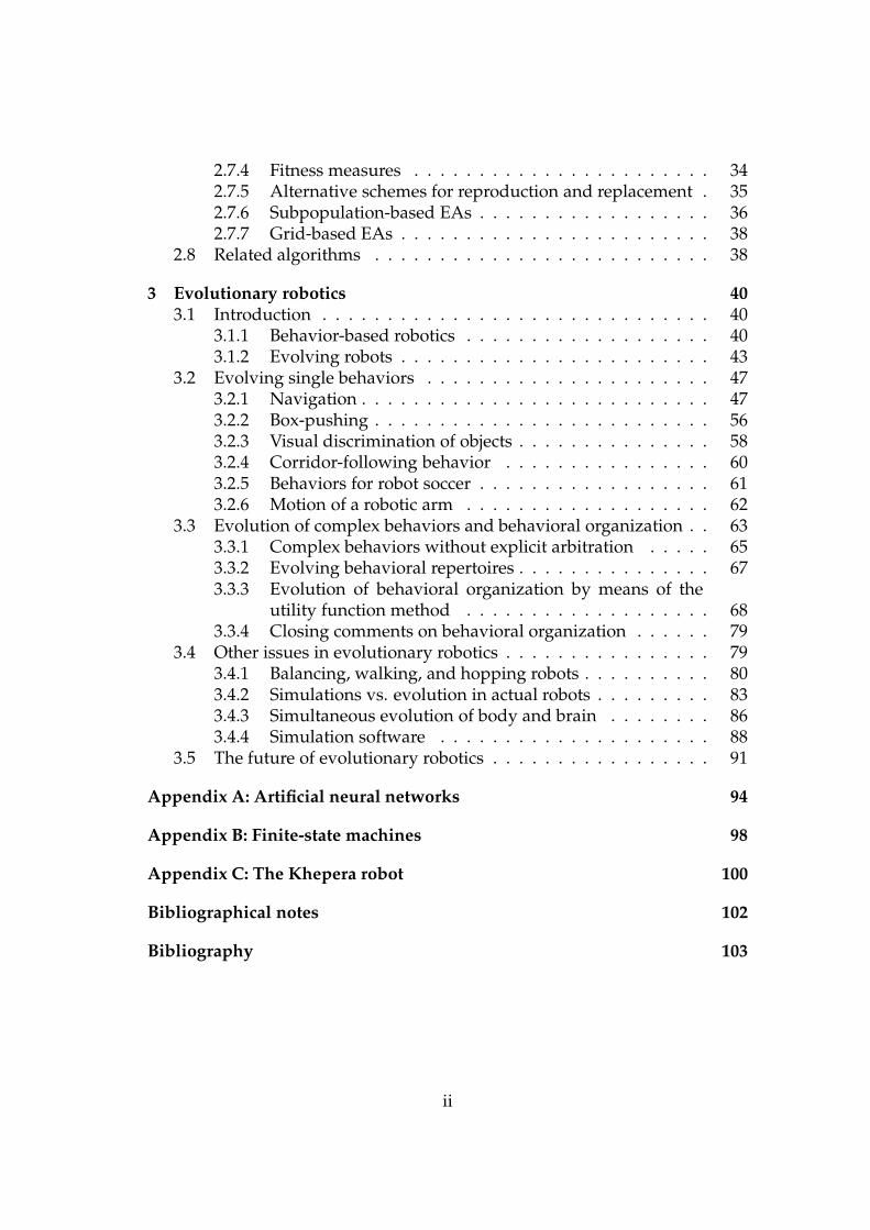
In this section, a brief introduction to ER will be given through a simple ex-ample, namely the evolution of a cleaning behavior. Consider an arena of thekind shown in the left panel of Fig. 1.1. The large cylinder represents a sim-ple, differentially steered, simulated two-wheeled robot, whereas the smaller(stationary) objects are considered to be garbage, and are to be removed by therobot. The aim is to use an evolutionary algorithm to generate a brain capableof making the robot clean the arena.
1.3.1 Cleaning behavior in simulation
The first choice that must be made is whether to evolve robotic brains in sim-ulation, or directly in hardware (an issue that will be discussed further in Sub-sect. 3.4.2). For the simple problem described here, which was part of an
Introduction 4
Figure 1.1: A simple, simulated cleaning robot (the large, circular object) in action [137].The initial state is shown in the left panel, and the final state in the right panel.
investigation concerning elementary behavioral selection [137], the choice wasmade to use simulated robots during evolution, and then attempt to transferthe best robotic brain found in simulation to a physical robot.
Next, a representation must be chosen for the robotic brains. Ideally, theEA should be given as much flexibility as possible but, in practice, some limi-tations must generally be introduced. In this problem, the robotic brains wererepresented as a generalized finite-state machines (GFSMs, see Appendix B),and the EA acted directly on the GFSMs rather than on a chromosomal encod-ing of them (see Sect. 2.7.2). In the beginning of the simulation, the GFSMswere small (i.e. contained very few states). However, the EA was allowed tochange the sizes of the GFSMs during the simulation.
The simulated robot was equipped with very simple sensors that coulddistinguish garbage objects from walls, but not much more.
The next step in the application of an EA is to choose a suitable fitnessmeasure, i.e. a performance measure for the evolving robotic brains. In theparticular case considered here, the aim of the robot was to place the garbageobjects as far from the center of the arena as possible. Thus, the fitness measurewas simply chosen as the mean square distance, counted from the center of thearena, of all the garbage objects at the end of the evaluation.
Furthermore, each robot was evaluated against several (usually five) differ-ent starting configurations, with garbage objects placed in different positions,to avoid a situation where the evolved robot would learn only to cope with agiven configuration.
Next, an EA was set up, in which a population of robotic brains (in the formof GFSMs) was generated. As the EA progressed, evaluating robotic brains,and generating new ones using selection, crossover, and mutations (see Sect.2.5), better and better results were obtained. In early generations, the simu-lated robots did little more than run around in circles near their starting po-

Fundamentals of evolutionary methods 5
sition. However, some robots were lucky enough to hit one or a few garbageobjects, thereby moving them slightly towards the walls of the arena. Beforelong, there appeared robots that would hit all the garbage objects.
The next evolutionary leap led to purposeful movement of objects. Here, aninteresting method appeared: Since both the body of the robot and the garbageobjects were round, objects could not easily be moved forward; Instead, theywould slide away from the desired direction of motion. Thus, a method in-volving several states of the GFSM was found, in which the robot moved in azig-zag fashion, thus managing to keep the garbage object in front.
Next, robots appeared that were able to deliver a garbage object at a wall,and then return towards the center of the arena in a curved, sweeping motion,in order to detect objects remaining near the center of the arena.
Towards the end of the run, the best evolved robots were able to place all, oralmost all, garbage objects near a wall, regardless of the starting configuration.
An example of the motion of an evolved robot is provided on the CD asso-ciated with the tutorial, in the file Cleaning_Simulation.avi .
1.3.2 Cleaning behavior in a Khepera robot
Needless to say, the aim of ER is to generate real, physical robots capable ofperforming useful tasks. Simulation is a useful tool in ER, but the final resultsshould be tested in physical robots.
The simulations for the cleaning robot discussed above were, in fact, stronglysimplified, and no attempt was made to simulate a physical robot exactly.Nevertheless, the best robotic brain obtained in the simulations was adaptedfor the Khepera robot (see Appendix C), the adaptation consisting mainly ofrescaling the parameters of the robotic brain, such as e.g. wheel speeds andsensor readings, to appropriate ranges. Quite amazingly, the evolved roboticbrain worked almost as well in the Khepera robot as in the simulated robots,as can be seen in the film Cleaning_Khepera.avi , which is also availableon the tutorial CD. Thus, in this particular case, the transition from simulationto real robots was quite simple, probably due to the simplicity of the problem.However, despite its simplicity, the problem just described still illustrates thepower of EAs as a method for generating robotic behaviors. Now, before pro-ceeding with a survey of results obtained in the field of ER, an introduction toEAs will be given.

Chapter 2
Fundamentals of evolutionaryalgorithms
2.1 Introduction
EAs are methods for search and optimization, (loosely) based on the propertiesof darwinian evolution. Typically, EAs are applied in optimization problemswhere classical optimization methods, such as e.g. gradient descent, Newton’smethod etc. [1] are difficult or impossible to apply. Such cases occur when theobjective function (i.e. the function whose maximum or minimum one wantsto find) is either not available in analytical form or is very complex (combining,say, thousands of real-valued and integer-valued variables).
Since the introduction of EAs in the 1970s, the number of applications ofsuch algorithms has grown steadily, and EAs are today used in fields as diverseas engineering, computational biology, finance, astrophysics, and, of course,robotics.
Below, a brief introduction to EAs will be given. Clearly, it is impossible toreview completely the vast topic of EAs on a few pages. Thus, readers inter-ested in learning more about EAs should consult other sources as well, e.g. [4],[51], [84], and [88].
Before introducing EAs, however, it is necessary to give a brief introduc-tion to the terms and concepts that appear in the study of biological evolution.Needless to say, this, too, is a vast topic, and only the most basic aspects willbe given below. For more information on biological evolution, see e.g. [22] and[23]. As their name implies, EAs are based on processes similar to those thatoccur during biological evolution. A central concept in the theory of evolutionis the notion of a population, by which we mean a group of individuals of thesame species (i.e. that can mate and have fertile offspring), normally confinedto some particular area in which the members of the population live, repro-duce, and die. The members of the population are referred to as individuals.
6

Fundamentals of evolutionary methods 7
In cases where members of the same species are separated by, for instance, abody of water or a mountain range, they form separate populations. Givenenough time, speciation (i.e. the formation of new species) may occur.
One of the central ideas behind Darwin’s theory of evolution is the idea ofgradual, hereditary change: New features in a species, such as protective coveror fangs, evolve gradually in response to a challenge provided by the environ-ment. For instance, in a species of predators, longer and sharper fangs mayevolve as a result of the evolution of thicker skin in their prey. This gradualarms race between two species is known as co–evolution.
The central concept is heredity, i.e. the idea that the properties of an indi-vidual can be encoded in such a way that they can be transmitted to the nextgeneration when (and if) an individual reproduces. Thus, each individual ofa species carries a genome that, in higher animals, consists of several chromo-somes in the form of DNA molecules. Each chromosome, in turn, containsa large number of genes, which are the units of heredity and which encodethe information needed to build and maintain an individual. Each gene iscomposed, essentially, of a sequence of bases. There are four bases in chro-mosomes (or DNA molecules), denoted A,C,G, and T. Thus, the informationis stored in a digital fashion, using an alphabet with four symbols. Duringdevelopment, as well as during the life of an individual, the DNA is read byan enzyme called RNA polymerase, and this process, known as transcriptionproduces messenger RNA (mRNA). Next, proteins are generated in a processcalled translation, using mRNA as a template.
Proteins are the building blocks of life, and are involved in one way oranother in almost every activity that takes place inside the living cell.
Each gene can have several settings. As a simple example, consider a genethat encodes eye color in humans. There are several options available: Eyesmay be green, brown, blue etc. The settings of a gene are known as alleles. Ofcourse, not all genes encode something that is as easy to visualize as eye color.The complete genome of an individual, with all its settings (encoding e.g. haircolor, eye color, height etc.) is known as the genotype.
During development, the stored information is decoded, resulting in anindividual carrying the traits encoded in the genome. The individual, with allits traits, is known as the phenotype, corresponding to the genotype.
Two central concepts in evolution are fitness and selection (for reproduc-tion), and these concepts are often intertwined: Individuals that are well adap-ted to their environment (which includes not only the climate and geographyof the region where the individual lives, but also other members of the samespecies, as well as members of other species), i.e. those that are stronger ormore intelligent than the others, have a larger chance to reproduce, and thusto spread their genetic material, resulting in more individuals having theseproperties etc.
Reproduction is the central moment for evolutionary change. Simplifying

Fundamentals of evolutionary methods 8
0 1 0 1 1 0 1 1 0 1 0 1 0 1 1 0 1 0 0 0 0 1 1 0 1 1 0 1 1 1 0 1 0 1 0 0 1 0 0 0 1 1 0 1 1 1 0 1 1 0 1 1 0 1
X , X1 2
Figure 2.1: Typical usage of a chromosome in a genetic algorithm. The 0s and 1s are thegenes, which are used as binary numbers to form, in this case, two variables x1 and x2, usinge.g. the first half of the chromosome to represent x1 and the second half to represent x2.
somewhat, we may say that during this process, the chromosomes of two (inthe case of sexual reproduction) individuals are combined, some genes beingtaken from one parent and others from the other parent. The copying of ge-netic information takes place with remarkable accuracy, but nevertheless thereoccurs some errors. These errors are known as mutations, and constitute theproviders of new information for evolution to act upon. In some simple species(e.g. bacteria) sexual reproduction does not occur. Instead, these species useasexual reproduction, in which only one parent is involved.
2.2 Biology vs. evolutionary algorithms
It should be noted that the description of reproduction above (and indeed ofevolution altogether) is greatly simplified: For example, in higher animals,the chromosomes are paired, allowing such concepts as recessive traits etc.Furthermore, not all parts of DNA are actually used in the production of anindividual: A large part of the genetic information is dormant (but may cometo be used in later generations).
Another simplification, relevant to the topic of EAs, comes from the waychromosomes are used. The most common usage in EAs is illustrated in Fig. 2.1.The figure shows the typical procedure used when generating an individualfrom a chromosome in a genetic algorithm As can be seen from the figure,the chromosome is used as a lookup table from which the traits of the corre-sponding individual are obtained. In the simple case shown in the figure, theindividual obtained consists of two variables x1 and x2 which can be used e.g.in a function optimization problem.
2.2.1 Embryological development
The simple procedure shown in Fig. 2.1 is, in fact, just a caricature of the pro-cess taking place when an individual is generated in a biological systems. Thebiological process is illustrated schematically in Fig. 2.2. First of all, in biolog-
Fundamentals of evolutionary methods 9
1 2 3 4
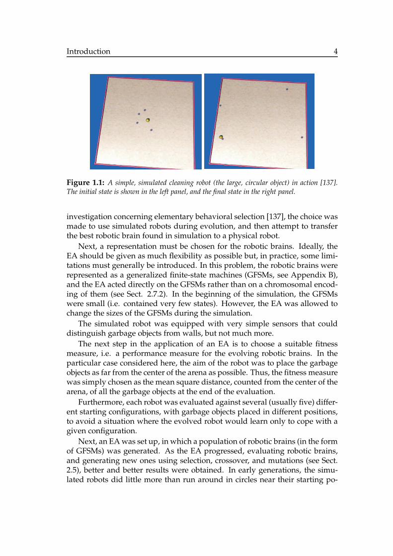
Figure 2.2: A schematic illustration of the function of the genome in a biological system.Four genes are shown. Genes 1, 3, and 4 are transcription factors, which regulate each other’slevels of expression, as well as that of gene 2, which is a structural gene. The arrow below gene2 indicates that its product is used in the cell for some other purpose than gene regulation. Notethat the figure is greatly simplified in that the intermediate step of translation is not shown.
ical systems, the chromosome is not used as a simple lookup table. Instead,genes interact with each other to form complex genetic regulatory networks,in which the activity (i.e. the level of production of mRNA) of a gene oftenis regulated by the activity of several other genes [109]. In such cases, theproduct of a gene (i.e. a protein) may attach itself to an operator close (on theDNA molecule) to another gene, and thereby affect, i.e. increase or decrease,the ability of RNA polymerase to bind to the DNA molecule at the startingposition of the gene (the promoter region).
Genes that regulate other genes are called regulatory genes or transcrip-tion factors. Some regulatory genes regulate their own expression, forminga direct feedback loop, which can act to keep the activity of the gene withinspecific bounds (see gene 1 in Fig. 2.2).
Gene regulation can occur in other ways as well. For example, a regulatorygene may activate a protein (i.e. the product of another gene) which then,in turn, may affect the transcription of other genes. Genes that have othertasks than regulatory ones are called structural genes. Such genes producethe many proteins needed for a body to function, e.g. those that appear inmuscle tissues. In addition, many structural genes code for enzymes, whichare proteins that catalyze various chemical reactions, such as, for example,breakdown of sugars.
During embryological development of an individual, the genome thus ex-ecutes a complex program, resulting in a complete individual.
2.2.2 Multicellularity
An additional simplification in most EAs is the absence of multicellularity. Bycontrast, in biological systems, the development of an individual results in asystem of many cells (except, of course, in the case of unicellular organisms),

Fundamentals of evolutionary methods 10
and the level of gene expression in each cell is determined by its interactionwith other cells. Thus, signalling between cells is an important factor in bio-logical systems. Note, however, that the set of chromosomes, and therefore theset of genes, is the same in all somatic (non-germ) cells in a biological organism.It is only the expression of genes that varies between cells, determining e.g. if acell should become part of the brain (a neuron) or part of the muscle tissue.
2.2.3 Gene regulation in adult animals
In EAs, the individual resulting from the decoding procedure shown in Fig. 2.1is usually fixed during its evaluation. However, in biological systems, thegenome remains active throughout the life time of the individuals, and con-tinues to produce the proteins needed in the body. In a computer analogy, theembryological development described above can be considered as a subrou-tine which comes to a halt when the individual is born. At that time, anothersubroutine, responsible for the growth of the newborn individual is activated,and is finally followed by a subroutine active during adult life. The amountneeded of any given protein usually varies with time, and continuous generegulation is thus essential in biological organisms.
2.2.4 Summary
To summarize the description of evolution, it can be noted that it is a processthat acts on populations of individuals. Information is stored in the individ-uals in the form of chromosomes, consisting of many genes. Individuals thatare well adapted to their environment are able to initiate the formation of newindividuals through the process of reproduction, which combines the geneticinformation of two separate individuals. Mutations provide further materialfor the evolutionary process.
Finally, it should be noted that, while EAs are inspired by biological evolu-tion, they often represent a strong simplification of the very complex processesoccurring in biological evolution. Clearly, there is no need to reproduce biol-ogy exactly: In ER, the aim is to generate e.g. artificial brains for autonomousrobots by means of any method that allows one to do so, and there is nothingpreventing deviations from biology.
2.3 Taxonomy of evolutionary algorithms
The taxonomy of EAs is sometimes confusing, particularly since different au-thors sometimes use slightly different definitions of the particular version ofEAs they are using. Here, EAs will be considered the umbrella term, coveringall types of algorithms based on darwinian evolution. A common special case
Fundamentals of evolutionary methods 11
Allindividualsevaluated?
No
Initialize population
Yes
Satisfactoryresult obtained?
Decode chromosome Evaluate individual
Select two individuals Perform crossover Mutate
Newpopulationcomplete?
No
Terminate run
Insert the two newindividuals in thepopulation
Replace entire parentpopulation by offspring
Yes
No
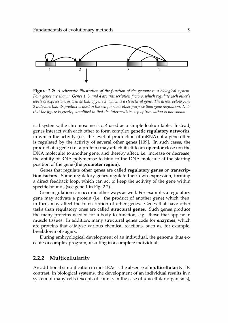
Figure 2.3: The basic flow of a standard GA, using generational replacement (see Sub-sect. 2.5.4 below). The dashed arrow indicates that crossover is only carried out with a proba-bility pc.
are genetic algorithms (GAs) [51], in which the variables of the problem areencoded in strings of digits which, when decoded, generate the system that isto be optimized (e.g. the brain of a robot represented, for example, by a neuralnetwork). Another version of EAs are evolution strategies (ESs) [5]. In a tra-ditional ES, the variables of the problem were encoded as numbers taking anyvalue in a given range (e.g. [0, 1]), whereas in traditional GAs, the digits wereusually binary, i.e. either 0 or 1. There were other differences as well, such asthe use of a variable mutation rate in ESs, whereas GAs typically used a con-stant mutation rate. However, GAs and ESs have gradually approached eachother, and many practitioners of EAs today use real-valued encoding schemesand variable mutation rates in algorithms which they refer to as GAs.
Other versions exist as well, and they differ from the traditional GA mainlyin the representations used. Thus, in genetic programming (GP) [68], the rep-resentation is usually a tree-like structure (even though a more recent version,linear GP, uses a representation closer to that used in GAs, further blurring thedistinction between different algorithms). In evolutionary programming (EP)[38], a representation in the form of finite-state machines (see Appendix B) wasoriginally used.
While there are many different versions of EAs, all such algorithms sharecertain important features - they operate on a population of candidate solu-

Fundamentals of evolutionary methods 12
tions (individuals), they select individuals in proportion to their performance,and then apply various operators (the exact nature of which depends on therepresentation used) to form new individuals, providing a path of gradual,hereditary change towards the desired structure.
In evolutionary robotics, it is common to skip the step of encoding the infor-mation in strings of digits, and instead allow the EA act directly on the struc-ture being optimized. For example, in the author’s research group, EAs areoften used that operate directly on recurrent neural networks (see AppendixA) or even on a behavioral selection system. The optimization of such systemswill be discussed below. In general, a system being optimized by an EA willbe called a structure whether or not it is obtained by decoding a chromosome.Thus, in a GA, one may optimize, say, a structure such as a neural network offixed size, obtained from a chromosome. Alternatively, one may use a moregeneric type of EA, in which the encoding step is skipped, and the EA insteadacts directly on the neural network.
2.4 Basic operation of evolutionary algorithms
Before discussing the various components of EAs, a brief description of the ba-sic functionality of such algorithms will be given, centered around the exam-ple of function optimization using a standard GA. However, with only smallmodifications, the discussion is applicable to almost any EA. The basic flowof a GA is shown in Fig. 2.3. The first step of any EA (not shown in the fig-ure), is to select a representation for the structures on which the algorithm willact. In the standard GA, the structures are strings of (binary) digits, knownas chromosomes. An example of a chromosome is shown in Fig. 2.1. Whendecoded, the chromosome will generate the corresponding individual, i.e. thephenotype corresponding to the genotype given by the chromosome. In thecase shown in Fig. 2.1, the individual simply consists of two real numbers x1
and x2, but more complex structures, such as e.g. ANNs, can also be encodedin chromosomes. In the case of ANNs, the real numbers obtained from thechromosome can be used for representing network weights.
As mentioned above, the encoding-decoding step is sometimes skipped inER. However, for the remainder of this section, only encoding schemes mak-ing used of chromosomes, represented as linear strings, will be considered.Advanced topics, such as EAs operating directly on a complex structure (e.g.an ANN), or using structures of variable size, will be considered in Sect. 2.7.2.
Once a representation has been chosen, the next step is to initialize the chro-mosomes, which is normally done in a random fashion. Next, each chromo-some is decoded to form the corresponding individual, which is then evalu-ated and assigned a fitness value, specified by the user. Consider the specific

Fundamentals of evolutionary methods 13
Figure 2.4: The function ψ10. The surface shows the function values obtained while keepingx3, x4, . . . , x10 fixed at zero, and thus only varying x1 and x2.
case of function maximization, applied to the benchmark function
ψn(x1, x2, . . . , xn) =1
2+
1
2nexp (−α
n∑
i=1
x2i )
n∑
i=1
cos
(
β√ixi
i∑
j=1
jxj
)
, (2.1)
where α and β are constants. This function has a global maximum of 1 atx1 = x2 = . . . = xn = 0, and is illustrated in Fig. 2.4 for the case n = 10,and with α = 0.05, β = 0.25. The figure was generated using the programGA Function Maximizer v1.1 , which is provided on the CD associatedwith this tutorial. The fitness measure should be such that individuals thatcome close to the desired result receive higher fitness than those that do not.Thus, in the case of function maximization, a possible fitness measure is simplythe function value itself1. Thus, for each individual, the variables x1, x2, . . . xn
are obtained from the chromosome, and the fitness value f = ψn(x1, x2, . . . , xn)is computed.
Following the flow chart in Fig. 2.3, when all individuals have been eval-uated, the production of new individuals can begin. Here, the first step isto select two (in case of sexual reproduction) individuals from the population,which will be used as parents for two new individuals. In general, the selectionof individuals is performed in a fitness-proportional manner, thus favoring in-dividuals with high fitness while at the same time allowing for the selection ofless fit individuals. The details of various selection procedures will be givenbelow in Subsect. 2.5.3. When two parents have been selected, two new indi-viduals are formed, normally using crossover with a certain probability pc (thecrossover probability, in which the genetic material of the parents is mixed,and mutation, in which a small, random change is made to each of the two
1In case of minimization, the inverse of the function value can be used.

Fundamentals of evolutionary methods 14
new chromosomes. The crossover and mutation operators are described inSubsects. 2.5.5 and 2.5.6 below. The procedure is repeated N/2 times, whereN is the population size. The N new individuals thus generated replace theN individuals from which parents were selected, forming the second genera-tion, which is evaluated in the same way as the first generation (see the flowchart). The whole procedure - evaluation, selection, crossover, and mutation -is repeated until a satisfactory solution to the problem has been found.
2.5 Basic components of evolutionary algorithms
Following the schematic example above, the main components of EAs willnow be described in some detail. For a more detailed description, see e.g.[4], [84], and [88]. Note that the implementation of some operators, notablycrossover and mutation, depends on the particular representation used.
2.5.1 Encoding schemes
The representation of the chromosomes can be chosen in several different ways.In the standard GA, binary encoding is used. Another alternative is real–number encoding, where genes take any value in the range [0, R], where Ris a non-negative real number (usually 1). As is often the case with EAs, it isnot possible to say that one encoding scheme is always superior to the others,and it is also difficult to make a fair comparison between the various encodingschemes. Real–number encoding schemes often use slightly different muta-tion methods (see below), which improve their performance in a way that isnot directly available for binary encoding schemes. In real–number encoding,a single gene g is used to represent a number between 0 and 1. This number isthen rescaled to the appropriate range ([−d, d]), according to
x = −d+ 2dg, (2.2)
assuming that the standard value R = 1 has been chosen for the range ofallowed gene values. For standard binary encoding, the procedure is
x = −d+ 2d(
g1 × 2−1 + g2 × 2−2 + g3 × 2−3 + . . .)
, (2.3)
where gi denotes the ith gene used in the representation of the variable x. Thereare also other procedures for encoding numbers using binary chromosomes.An example is Gray coding, which will be discussed briefly in Sect. 2.7.1.
2.5.2 Fitness assignment
The simplest possible fitness assignment consists of simply assigning the valueobtained from the evaluation (assuming a maximization task) without any

Fundamentals of evolutionary methods 15
transformations. This value is known as the raw fitness value. For example,if the task is to find the maximum of a simple trigonometric function such asf(x) = 1 + sin(x) cos(2x), the raw fitness value would be useful. However, ifinstead the task is to find the maximum of the function g(x) = 1000+ f(x), theraw fitness values would be of little use, since they would all be of order 1000.The selection process would find it difficult to single out the best individuals.
It is therefore generally a good idea to rescale the fitness values before theyare used. Linear fitness ranking is a commonly used rescaling procedure,where the best of the N individuals in the population is given fitness N, thesecond best fitness N − 1 etc. down to the worst individual, which is givenfitness 1. Letting R(i) denote the ranking of individual i, defined such that thebest individual ibest has ranking R(ibest) = 1 etc. down to the worst individualwith ranking R(iworst) = N , the fitness assignment is given by
f(i) = (N + 1 −R(i)). (2.4)
Fitness ranking must be used with caution, however, since individuals that areonly slightly better than the others may receive very high fitness values andsoon come to dominate the population, trapping it in a local optimum. Thetendency to converge on a local optimum can be decreased by using a lessextreme fitness ranking, assigning fitness values according to
f(i) = fmax − (fmax − fmin)
(
R(i) − 1
N − 1
)
. (2.5)
This ranking yields equidistant fitness values in the range [fmin, fmax]. The sim-ple ranking in Eq. (2.4) is obtained if fmax = N, fmin = 1.
The choice of the fitness measure often has a strong impact on the resultsobtained by the GA, and the topic will be discussed further in Sect. 2.7.4.
2.5.3 Selection
Selection can be carried out in many different ways, two of the most com-mon being roulette-wheel selection and tournament selection. All selectionschemes preferentially select individuals with high fitness, while allowing se-lection of less fit individuals as well.
In roulette-wheel selection, two individuals are selected from the wholepopulation using a procedure in which each individual is assigned a slice of aroulette wheel, with an opening angle proportional to its fitness. As the wheelis turned, the probability of an individual being selected is directly propor-tional to its fitness. An algorithm for roulette-wheel selection is to draw a ran-dom number r between 0 and 1, and the select the individual correspondingto the smallest value j which satisfies the inequality
∑j
i=1 fi∑N
i=1 fi
> r, (2.6)

Fundamentals of evolutionary methods 16
where fi denotes the fitness of individual i.
It is evident that roulette-wheel selection is a far cry from what happensin nature, where small groups of individuals, usually males, fight each otheruntil there remains a single winner which is allowed to mate. Tournamentselection tries to incorporate the main features of this process. In its simplestform, tournament selection consists of picking two individuals randomly fromthe population, and then selecting the best one as a parent. When two parentshave been selected this way, crossover and mutation takes place as usual. Amore sophisticated tournament selection scheme involves selecting m individ-uals randomly from the population. Next, with probability r, the best of the mindividuals is selected, and with probability 1− r a random individual amongthe other m−1 is selected. m is referred to as the tournament size, and r is thetournament selection parameter. A typical numerical value for r is around0.75. The tournament size is commonly set as a (small) fraction of the popu-lation size. Thus, unlike the case with roulette-wheel selection, in tournamentselection no individual is discarded without at least participating in a closecombat involving a small number of individuals. Note also that, in tourna-ment selection, negative fitness values are allowed, whereas all fitness valuesin roulette-wheel selection must be non-negative.
Both roulette-wheel selection and tournament selection operate with re-placement, i.e. selected individuals are returned to the population and canthus be selected again.
2.5.4 Replacement
In the example described in the previous section, generational replacementwas used, meaning that all individuals in the evaluated generation were re-placed by an equal number of offspring. Generational replacement is not veryrealistic from a biological point of view. In nature, different generations co–exist and individuals appear (and disappear) constantly, not only at specificintervals of time. By contrast, in generational replacement, there is no compe-tition between individuals from different generations.
In general, replacement schemes can be characterized by their generationalgap G, which simply measures the fraction of the population that is replacedin each selection cycle, i.e. in each generation. Thus, for generational replace-ment, G = 1.
At the opposite extreme are replacement schemes that only replace one in-dividual in each step. In this case G = 1/N , where N is the population size.In steady-state reproduction, G is usually equal to 1/N or 2/N , i.e. one or twoindividuals are replaced in each generation. In order to keep the populationsize constant, NG individuals must be deleted. The deletion procedure variesbetween different steady-state replacement schemes; In some, only the N par-

Fundamentals of evolutionary methods 17
Figure 2.5: Single-point crossover as implemented in a standard GA using fixed-length chro-mosomes. The crossover point is selected randomly.
ents are considered for deletion, whereas in others, both parents and offspringare considered.
Deletion of individuals can be done in various ways, e.g. by removing theleast fit individuals or by removing the oldest individuals.
As mentioned above, for G = 1 (i.e. generational replacement), individualsfrom different generations do not compete with each other. Note however thatthere may still be some de facto overlap between generations if the crossoverand mutation rates are sufficiently low since, in that case, many of the offspringwill be identical to their parents.
2.5.5 Crossover
Crossover allows partial solutions from different regions of the search space tobe assembled into a complete solution to the problem at hand.
The crossover procedure can be implemented in various ways. The sim-plest version is one–point crossover, in which a single crossover point is ran-domly chosen, and the first part of the first chromosome is joined with thesecond part of the second chromosome, as shown in Fig. 2.5. The procedurecan be generalized to n–point crossover, where n crossover points are selectedrandomly, and the chromosome parts are chosen with equal probability fromeither parent. In uniform crossover, the number of crossover points is equalto the number of genes in the chromosome, minus one.
While crossover plays a very important role, its effects may be negative ifthe population size is small, which is almost always the case in artificial evo-lution where the population size N typically is of order 30–1,000, as comparedto populations of several thousands or even millions of individuals in nature.The problem is that, through crossover, a successful (partial) solution will veryquickly spread through the population causing it to become rather uniform oreven completely uniform, in the absence of mutation. Thus, the populationwill experience inbreeding towards a possibly suboptimal solution.
A possible remedy is to allow crossover or sexual reproduction only witha certain probability pc. In this case, some new individuals are formed us-ing crossover followed by mutation, and some individuals are formed usingasexual reproduction, in which only mutations are involved. pc is commonly

Fundamentals of evolutionary methods 18
chosen in the range [0.7, 0.9].
2.5.6 Mutation
In natural evolution, mutation plays the role of providing the two other mainoperators, selection and crossover, with new material to work with. Most of-ten, mutations are deleterious when they occur but may bring advantages inthe long run, for instance when the environment suddenly undergoes changessuch that individuals without the mutation in question have difficulties sur-viving.
In GAs, the value of the mutation probability pmut is usually set by the userat the start of the computer run, and is thereafter left unchanged throughoutthe simulation. A typical value for the mutation probability is around 1/n,where n is the number of genes in the chromosome. There are, however, someversions of EAs, notably evolution strategies, in which the mutation probabil-ities are allowed to vary, see e.g. [5].
In the case of chromosomes using binary encoding, mutation normally con-sists of changing the value of a gene to the complementary value, i.e. changingfrom 0 to 1 or from 1 to 0, depending on the value before mutation.
In real–number encoding, the modifications obtained by randomly select-ing new values often become too large to be useful and therefore an alterna-tive approach, known as real–number creep, is frequently used instead. Inreal–number creep, the mutated value is not completely unrelated to the valuebefore the mutation as in the discrete encodings. Instead, the mutation is cen-tered on the previous value and the creep rate determines how far the muta-tion may take the new value. In arithmetic creep, the old value g of the geneis changed to a new value g′ according to
g → g′ = g − c + 2cr, (2.7)
where c ∈ [0, 1] is the creep rate and r is a random number in [0, 1]. In geomet-ric greep, the old value of the gene changes as
g → g′ = g(1 − c+ 2cr), (2.8)
Note that, in geometric creep, the variation in the value of the gene is propor-tional to the previous value. Thus, if g is small, the change in g will be smallas well. In addition, it should be noted that geometric creep cannot changethe sign of g. Thus, when using geometric creep, the encoding scheme shouldbe the standard one for real-numbered encoding, in which genes take non-negative values (e.g. in [0, 1]).
Furthermore, in both arithmetic and geometric creep, it is possible to obtainnew values g′ outside the allowed range. In that case, g′ is instead set to thelimiting value.

Fundamentals of evolutionary methods 19
Finally, it should be noted that creep mutations can be defined for binaryrepresentations as well. One procedure for doing so is to decode the genesrepresenting a given variable, change the variable by a small amount, e.g. ac-cording to an equation similar to Eq. (2.7) or Eq. (2.8), and then to encode thenew number back into the chromosome.
2.5.7 Elitism
Even though a fit individual has a large probability of being selected for repro-duction, there is no guarantee that it will be selected. Furthermore, even if it isselected, it is probable that it will be destroyed during crossover or mutation.In order to make sure that the best individual is not lost, it is common to makeone or a few exact copies of this individual and place them directly in the nextgeneration, a procedure known as elitism. All the other new individuals areformed via the usual sequence of selection, crossover, and mutation.
2.6 Genetic programming
As mentioned in Sect. 2.3, there exists many different types of EAs. In ER, oneof the simplest methods of generating a robotic brain is to evolve the weightsof an ANN (see Appendix A) of fixed size, using a GA with direct encoding,illustrated in Fig. 2.6. In such an approach the network cannot change size, andits success or failure depends entirely on the experimenter’s ability to select anappropriate structure for the network.
More flexible approaches have also been developed, in which the size ofthe structure being optimized (be it an ANN or something else) is allowedto vary. Genetic programming (GP) is one such approach, and because of itsfrequent use in ER, a brief introduction will be given here. For a more thoroughintroduction, see e.g. [6] and [68].
In the original formulation of GP, which will be described first, tree-basedrepresentations were used for the individuals. In later versions, such as linearGP, simple, linear chromosomes have been used instead.
2.6.1 Tree-based genetic programming
As the name implies, tree-based GP is used for evolving combinations (trees)of elementary instructions, i.e. computer programs rather than strings of dig-its. Very often, GP is implemented using the LISP programming language,whose structure fits well with the tree–like structure of individuals in standardGP. However, GP can also be implemented in other programming languages.In tree-based GP, trees consisting of elementary operators and terminals aregenerated. The elementary operators require a number of input arguments,

Fundamentals of evolutionary methods 20
Weights and bias, neuron 1 Weights and bias, neuron 2 Weights and bias, neuron 3
+1
+1
+1
1
2
3
Figure 2.6: Direct encoding of a simple ANN with three neurons and two input elements.The weights and biases (the latter shown as vertical arrows) are obtained directly from thechromosome, which is used simply as a lookup table. In this case, an ordinary GA would be anappropriate technique for optimizing the ANN.
*
3 +
z *
5 *
z z
IfObjectInView
ChangeSpeed Turn
1 30
Figure 2.7: Two GP trees. The tree to the left can be decoded to the function f(z) = 3(z +5z2). The tree to the right tells a robot to increase its speed by one unit if it sees an object, andto turn by 30 degrees if it does not see any object.
Fundamentals of evolutionary methods 21
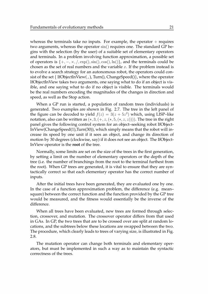
whereas the terminals take no inputs. For example, the operator + requirestwo arguments, whereas the operator sin() requires one. The standard GP be-gins with the selection (by the user) of a suitable set of elementary operatorsand terminals. In a problem involving function approximation, a possible setof operators is {+,−,×, /, exp(), sin(), cos(), ln()}, and the terminals could bechosen as the set of real numbers and the variable x. If the problem instead isto evolve a search strategy for an autonomous robot, the operators could con-sist of the set { IfObjectInView( , ), Turn(), ChangeSpeed()}, where the operatorIfObjectInView takes two arguments, one saying what to do if an object is vis-ible, and one saying what to do if no object is visible. The terminals wouldbe the real numbers encoding the magnitudes of the changes in direction andspeed, as well as the Stop action.
When a GP run is started, a population of random trees (individuals) isgenerated. Two examples are shown in Fig. 2.7. The tree in the left panel ofthe figure can be decoded to yield f(z) = 3(z + 5z2) which, using LISP–likenotation, also can be written as (∗, 3, (+, z, (∗, 5, (∗, z, z)))). The tree in the rightpanel gives the following control system for an object–seeking robot IfObject-InView(ChangeSpeed(1),Turn(30)), which simply means that the robot will in-crease its speed by one unit if it sees an object, and change its direction ofmotion by 30 degrees (clockwise, say) if it does not see an object. The IfObject-InView operator is the root of the tree.
Normally, some limits are set on the size of the trees in the first generation,by setting a limit on the number of elementary operators or the depth of thetree (i.e. the number of branchings from the root to the terminal furthest fromthe root). When GP trees are generated, it is vital to ensure that they are syn-tactically correct so that each elementary operator has the correct number ofinputs.
After the initial trees have been generated, they are evaluated one by one.In the case of a function approximation problem, the difference (e.g. mean–square) between the correct function and the function provided by the GP treewould be measured, and the fitness would essentially be the inverse of thedifference.
When all trees have been evaluated, new trees are formed through selec-tion, crossover, and mutation. The crossover operator differs from that usedin GAs. In GP, the two trees that are to be crossed over are split at random lo-cations, and the subtrees below these locations are swapped between the two.The procedure, which clearly leads to trees of varying size, is illustrated in Fig.2.8.
The mutation operator can change both terminals and elementary oper-ators, but must be implemented in such a way as to maintain the syntacticcorrectness of the trees.

Fundamentals of evolutionary methods 22
Figure 2.8: The crossover procedure in tree-based GP.
2.6.2 Linear genetic programming
Unlike tree-like GP, linear GP (LGP) [13] is used for evolving linear sequencesof basic instructions defined in the framework of an imperative programminglanguage.2 Two central concepts in LGP are registers and instructions. Reg-isters are of two basic kinds, variable registers and constant registers. Theformer can be used for providing input, manipulating data, and storing theoutput resulting from a calculation. As a specific example, consider the ex-pression
r3 := r1 + r2; (2.9)
In this example, the instruction consists of assigning a variable register (r3 ) thesum of the contents in two other variable registers (r1 and r2 ). As a secondexample, consider the instruction
r1 := r1*c1; (2.10)
Here, a variable register r1 , is assigned its previous value multiplied by thecontents of a constant register c1 . In LGP, a sequence of instructions of thekind just described are specified in a linear chromosome. The encoding schememust thus be such that it identifies the two operands (i.e. r1 and c1 in the sec-ond example above), the operator (multiplication, in the second example), aswell as the destination register (r1 ). An LGP instruction can thus be repre-sented as a sequence of integers that identify the operator, the index of thedestination registers, and the indices of the registers used as operands. Forexample, if only the standard arithmetic operators (addition, subtraction, mul-tiplication, and division) are used, they can be identified e.g. by the numbers
2In imperative programming, computation is carried out in the form of an algorithm con-sisting of a sequence of instructions. Typical examples of imperative programming languagesare C, Fortran, Java, and Pascal, as well as the machine languages used in common micropro-cessors and microcontrollers. By contrast, declarative programming involves a description ofa structure but no explicit algorithm (the specification of an algorithm is left to the support-ing software that interprets the declarative language). A web page written in HTML is thusdeclarative.

Fundamentals of evolutionary methods 23
Instruction Description Instruction DescriptionAddition ri := rj + rk Sine ri := sin rj
Subtraction ri := rj − rk Cosine rj := cos rj
Multiplication ri := rj × rk Square ri := r2j
Division ri := rj/rk Square root ri :=√rj
Exponentiation ri := erj Conditional branch if ri > rj
Logarithm ri := ln rj Conditional branch if ri ≤ rj
Table 2.1: Examples of typical LGP operators. Note that the operands can be either variableregisters or constant registers.
1,2,3, and 4. The set of all allowed instructions is called the instruction setand it may, of course, vary from case to case. However, no matter which in-struction set is employed, the user must make sure that all operations generatevalid results. For example, divisions by zero must be avoided. Therefore, inpractice, protected definitions are used. An example of a protected definitionof the division operator is
ri :=
{
rj/rk if rk 6= 0,rj + cmax otherwise,
(2.11)
where cmax is a large (pre-specified) constant. Note that the instruction set can,of course, contain operators other than the simple arithmetic ones. Some ex-amples of common LGP instructions are shown in Table 2.1. The usage of thevarious instructions should be clear except, perhaps, in the case of the branch-ing instructions. Commonly, these instructions are used in such a way that thenext instruction is skipped unless the condition is satisfied. Thus, for example,if the following two instructions appear in sequence
if (r1 < r2)r1 := r2 + r3;
(2.12)
the value of r1 will be set to r2+r3 only if r1 < r2 when the first instructionis executed. Note that it is possible to use a sequence of conditional branchesin order to generate more complex conditions. Clearly, conditional branchingcan be augmented to allow e.g. jumps to a given location in the sequence of in-structions. However, the use of jumping conditions can raise significantly thecomplexity of the representation. As soon as jumps are allowed, one faces theproblems of (1) making sure that the program terminates, i.e. does not enter aninfinite loop, and (2) avoiding jumps to non-existent locations. In particular,application of the crossover and mutation operators (see below) must then befollowed by a screening of a newly generated program, to ascertain that theprogram can be executed correctly. Jumping instructions will not be consid-ered further here.

Fundamentals of evolutionary methods 24
1 2 1 4 1 3 2 2 3 1 2 3 5 1 5 1 1 1 1 4
Operator (range [1,5])
Destination register (range [1,3])
Operand 1 (range [1,6])
Operand 2 (range [1,6])
Figure 2.9: An example of an LGP chromosome.
Genes Instruction Result1, 2, 1, 4 r2 := r1 + c1 r1 = 1, r2 = 2, r3 = 01, 3, 2, 2 r3 := r2 + r2 r1 = 1, r2 = 2, r3 = 43, 1, 2, 3 r1 := r2 × r3 r1 = 8, r2 = 2, r3 = 45, 1, 5, 1 if (r1 > c2) r1 = 8, r2 = 2, r3 = 41, 1, 1, 4 r1 := r1 + c1 r1 = 9, r2 = 2, r3 = 4
Table 2.2: Evaluation of the chromosome shown in Fig. 2.9, in a case where the input registerr1 was initially assigned the value 1. The variable registers r2 and r3 were both set to 0, andthe constant registers were set as c1 = 1, c2 = 3, c3 = 10. The first instruction (top line) isdecoded from the first four genes in the chromosome etc. The resulting output was taken as thevalue contained in r1 at the end of the calculation.
In LGP, chromosomes are used, similar to the those employed in a GA. Anexample of an LGP chromosome is shown in Fig. 2.9. Note that some instruc-tions (e.g. addition) need four numbers for their specification, whereas others(e.g. exponentiation) need only three. However, in order to simplify the rep-resentation, one may still represent each instruction by four numbers, simplyignoring the fourth number for those instructions where it is not needed. Notethat the four numbers constituting an instruction may have different range.For example, the operands may involve both variable registers and constantregisters, whereas the destination register must be a variable register. In thespecific example shown in Fig. 2.9, there are three variable registers available(r1, r2, and r3) and three constant registers (c1, c2, and c3), as well as five op-erators, namely addition, subtraction, multiplication, division, and the condi-tional branch instruction ’if (ri > rj)’. Let R denote the set of variable registers,i.e. R = {r1, r2, r3}, and C the set of constant registers, i.e. C = {c1, c2, c3}. LetA denote the union of these two sets, so that A = {r1, r2, r3, c1, c2, c3}. The setof operators, finally, is denoted O. Thus, in the set O = {o1, o2, o3, o4, o5}, thefirst operator (o1) represents + (addition) etc. An instruction is encoded usingfour numbers. The first number, in the range [1,5], determines the operator
Fundamentals of evolutionary methods 25
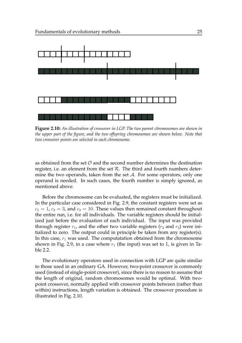
Figure 2.10: An illustration of crossover in LGP. The two parent chromosomes are shown inthe upper part of the figure, and the two offspring chromosomes are shown below. Note thattwo crossover points are selected in each chromosome.
as obtained from the set O and the second number determines the destinationregister, i.e. an element from the set R. The third and fourth numbers deter-mine the two operands, taken from the set A. For some operators, only oneoperand is needed. In such cases, the fourth number is simply ignored, asmentioned above.
Before the chromosome can be evaluated, the registers must be initialized.In the particular case considered in Fig. 2.9, the constant registers were set asc1 = 1, c2 = 3, and c3 = 10. These values then remained constant throughoutthe entire run, i.e. for all individuals. The variable registers should be initial-ized just before the evaluation of each individual. The input was providedthrough register r1, and the other two variable registers (r2 and r3) were ini-tialized to zero. The output could in principle be taken from any register(s).In this case, r1 was used. The computatation obtained from the chromosomeshown in Fig. 2.9, in a case where r1 (the input) was set to 1, is given in Ta-ble 2.2.
The evolutionary operators used in connection with LGP are quite similarto those used in an ordinary GA. However, two-point crossover is commonlyused (instead of single-point crossover), since there is no reason to assume thatthe length of original, random chromosomes would be optimal. With two-point crossover, normally applied with crossover points between (rather thanwithin) instructions, length variation is obtained. The crossover procedure isillustrated in Fig. 2.10.

Fundamentals of evolutionary methods 26
2.7 Advanced topics
In this section, a few advanced topics will be covered, with particular emphasison topics relevant to practitioners of ER. In should be noted that there is a verylarge number of variations on the theme of EAs. Thus, the description belowis intended as an illustration of a few advanced topics related to EAs, andis by no means exhaustive. The interested reader can find more informationconcerning advanced EA topics in e.g. [4].
2.7.1 Gray coding of binary-valued chromosomes
In the standard GA, a binary representation scheme is used in the chromo-somes. While simple to implement, such a scheme may have some disadvan-tages, one of them being that a small change in the decoded value obtainedfrom a chromosome may require flipping many bits which, in turn, is an un-likely event. Thus, the algorithm may get stuck simply as a result of the en-coding scheme. Consider, as an example, a ten-bit binary encoding scheme,and assume that the best possible chromosome is 1000000000. Now, considera case in which the population has converged to 0111111111. In order to reachthe best chromosome from this starting position, the algorithm would need tomutate all ten genes in the chromosome, even though the numerical differencebetween the decoded values obtained from the two chromosomes may be verysmall.
An alternative representation scheme, which avoids this problem is theGray code, which was patented in 1953 by Frank Gray at Bell Laboratories,but which had been used already in telegraphs in the 1870s. A Gray code issimply a binary representation of all the integers k, in the range [0, 2n], suchthat, in going from k to k + 1, only one bit changes in the representation. Thus,a Gray code representation of the numbers 0, 1, 2, 3 is given by 00, 01, 11, 10.
Of course, other 2-bit Gray code representations exist as well, for example10, 11, 01, 00 or 00, 10, 11, 01. However, these representations differ from theoriginal code only in that the binary numbers have been permuted or inverted.An interesting question is whether the Gray code is unique, if permutationsand inversions are disregarded. The answer turns out to be negative for n > 3.Gray codes can be generated in various ways.
2.7.2 Variable-size structures
In the standard GA, all chromosomes are of the same, fixed size, which is asuitable state of affairs for many problems. For example, in the optimizationof a function, with a known number of variables, it is easy to specify a chromo-some length. It is not entirely trivial, though: The number of genes per variablemust be set sufficiently high to give a representation with adequate accuracy

Fundamentals of evolutionary methods 27
for the variables. However, if the desired accuracy is difficult to determine,a safe approach is simply to set the number of genes per variable to a highvalue (50, say), and then run the GA with chromosomes of length 50 times thenumber of variables. Thus, there is no need to introduce chromosomes withvarying length.
However, in many other situations, it is desirable, or even essential, to op-timize structures of varying size. Indeed, during biological evolution, manydifferent genome sizes have resulted (in different species, both current and ex-tinct ones). Variations in genome length may result from accidents during theformation of new chromosomes, such as duplication of a gene or parts thereof(see Subsect. 2.7.5 below). Clearly, in nature, there can be no given, optimaland non-changing genome size. The same applies to artificial evolution ofcomplex structures, such as artificial brains for autonomous robots, whetherthe evolving structure is a behavioral selection system (see Sect. 3.3), a neuralnetwork (see Appendix A) or a finite-state machine (see Appendix B) repre-senting a single behavior, or some other structure. Evolutionary size variationcan be implemented either by allowing chromosomes to take variable lengthor by letting the EA act directly on the structure (e.g. a neural network) beingoptimized.
In general, varying size should be introduced in cases where there is insuf-ficient a priori knowledge of the optimal size of the structures being optimized.
In this section, two examples of encoding schemes will be given, startingwith a description of encoding schemes for ANNs. In view of their frequentuse in ER, ANNs occupy a central position in research concerning autonomousrobots, and therefore the description of ANNs will be quite detailed. However,the reader should keep in mind that there are also many cases in which archi-tectures other than ANNs are used in ER. For example, while ANNs are veryuseful for representing many individual behaviors in robots, other architec-tures are sometimes used when evolving behavioral selection (see Sect. 3.3).
Encoding schemes for neural networks
In the case of FFNNs (see Appendix A for the definition of network types)of given size, the encoding procedure is straightforward: If real-number en-coding is used, each gene can represent a network weight, and the decodingprocedure can easily be written so that it associates the weights with the cor-rect neuron. An example is shown in Fig. 2.6. Here, a simple FFNN withthree neurons, two in the hidden layer and one in the output layer is encodedin a chromosome containing 9 genes, shown as elongated boxes. If instead bi-nary encoding were to be used, each box would represent several genes which,when decoded, would yield the weight value.
In more complex applications, however, the encoding of information in alinear chromosome is often an unnecessary complication, and the EA can in-

Fundamentals of evolutionary methods 28
M1, M2 M3
M4
M6
M5
M7
Figure 2.11: Mutation operators (M1-M7). Modifications and additions are shown as boldlines and removed items are shown as dotted lines. The mutations are (M1-M2): weightmutations, either by a random value or a value centered on the previous value; (M3-M4):connectivity mutations, addition of an incoming weight with random origin (M3), or re-moval of an incoming weight (M4); (M5-M7): neuron mutations, removal of a neuron andall of its associated connections (M5), insertion of an unconnected neuron (zero-weight addi-tion) (M6), and addition of a neuron with a single incoming and a single outgoing connection(single connection addition) (M7). Reproduced with kind permission of Mr. J. Pettersson.
stead be made to operate directly on the structures that are to be optimized.For such implementations, object-oriented programming is very useful. Here,a type (i.e. a data structure) representing a neural network can be defined as alist of neurons, each of which is equipped with a list of incoming connectionsfrom input elements, as well as a list of incoming connections from neurons.Both the latter two lists and the list of neurons can then be allowed to vary insize. The generation of ANNs using EAs has been considered extensively inthe literature, see e.g. [146] for a review.
When generating brains for autonomous robots using EAs, there is rarelyany reason to limit oneself to FFNNs. Instead, the EA is commonly used foroptimizing completely general RNNs. Note, however, that the possibility ofgenerating an FFNN is not excluded, since such networks are special cases ofRNNs, and may appear as a result of the optimization procedure. When usingan EA to optimize RNNs of varying size, some problems must be tackled. Inparticular, several mutation operators must be defined, which can modify notonly the weights, but also the architecture (i.e. the structure) of the networks.A set of seven mutation operators (M1-M7) for RNNs is shown in Fig. 2.11.M1 and M2 modify the strengths of already present connections between units

Fundamentals of evolutionary methods 29
(see Appendix A) in the network, whereas M3-M7 modify the architecture ofthe network: M3 adds a connection between two randomly chosen units, andM4 removes an already present connection. M5 removes an entire neuron, andall its incoming and outgoing weights. M6 and M7 add neurons. In the caseof M6, the neuron is added without any incoming or outgoing weights. Thus,two mutations of type M3 are needed in order for the neuron to have an effecton the computation performed by the network. M7, by contrast, adds a neuronwith a direct connection from an input element to an output neuron (shownas filled circles in the figure). Note that many other neuron addition operatorscan be defined.
In addition, crossover operators can be defined that can combine chro-mosomes of varying size, unless the equivalent of species is introduced (seebelow), in which case only chromosomes of equal size are allowed in thecrossover procedure. In general, due to the distributed nature of computa-tion in neural networks, it is difficult to define a good crossover operator,even in cases where the networks are of equal size. This is so, since half anANN (say) does not perform half of the computation of the complete ANN.More likely, any part of an ANN will not perform any useful computationat all. Thus, cutting two networks in pieces and joining the first piece of thefirst network with the second piece of the second network (and vice versa) of-ten amounts to a huge macro-mutation, decreasing the fitness of the network,and thus generally eliminating it from the population. However, putting thisdifficulty aside for the moment, how should crossover be defined for neuralnetworks? One possibility is to encapsulate neurons, with their incoming con-nections into units, and only swap these units (using, e.g. uniform crossover)during crossover, rather than using a single crossover point.
Clearly, with this procedure, crossover can be performed with any two net-works. However, there is a more subtle problem concerning the identity of theweights. If the list of incoming weights to the neurons represents neuron in-dices, crossover may completely disrupt the network. For example, considera case where neuron 3, say, takes input from neurons 1, 4, and 5. If, duringcrossover, a single additional neuron is inserted between neurons 3 and 4, say,the inserted neuron will be the new neuron 4, and the old neuron 4 will becomeneuron 5 etc., thus completely changing the identities (and, therefore, the nu-merical values) of the weights, and also limiting the usefulness of crossover.
The problem of modified neuron identities can, of course, be mitigated bysimply rewiring the network (after e.g. neuron insertion) to make sure thatthe identities of the neurons and their weights remain unchanged. However,there are also biologically inspired methods for mitigating this problem: Con-sider another type of network, namely a genetic regulatory network. Here,some genes (transcription factors) can regulate the expression of other genes,by producing (via mRNA) protein products that bind to a binding site close tothe regulated genes. The procedure of binding is an ingenious one: Instead of,
Fundamentals of evolutionary methods 30
say, stating that e.g. ”the product of gene 45 binds to gene 32” (which wouldcreate problems like those discussed above, in the case of gene insertion ordeletion), the binding procedure may say something like ”the product of geneg binds to any gene with a binding site containing the nucleotide sequenceAATCGATAG”. In that case, if another gene, x say, is preceded (on the chro-mosome) by a binding site with the sequence AATCGATAG, the product ofgene g will bind to gene x regardless of their relative position on the chromo-some. Likewise, the connection can be broken if the sequence on the bindingsite preceding gene x is mutated to, say, ATTCGATCG. Encoding schemes us-ing neuron labels instead of neuron indices can be implemented for the evolu-tion of ANNs, but they will not be considered further here.
As mentioned above, crossover between networks often leads to lower fit-ness. However, there are crossover operators that modify networks more gen-tly. One such operator is averaging crossover, which can be applied to net-works of equal size. Consider a network of a given size, using an encodingscheme as that illustrated in Fig. 2.6. In averaging crossover, the value of genex in the two offspring, denoted x′1 and x′2 is given by
x′1 = αx1 + (1 − α)x2, (2.13)
andx′2 = (1 − α)x1 + αx2, (2.14)
where x1 and x2 denote the values of x in the parents. α is a number in therange [0, 1]. In case α is equal to 0 or 1, no crossover occurs, but for all othervalues of α there will be a mixing of genetic material from both individuals inthe offspring. If α is close to 0 (or 1), the mixing is very gentle.
Grammatical encoding
The introduction of variable-size structures, as discussed above, adds consid-erable flexibility to an EA, and is crucial in the solution of certain problems.
Another motivation for the introduction of variable-size structures is thefact that such structures have more similarity with chromosomes found innatural evolution. However, as was discussed in Sect. 2.2, even the variable-size structures used in EAs differ considerably from biological chromosomes.A particularly important difference is the fact that biological chromosomesdo not, in general, encode the parameters of a biological organism directly,whereas the structures (e.g. linear chromosomes) used in EAs most often douse such direct encoding.
An example should be given to illustrate the state of affairs in biologicalsystems. Consider the human brain. This very complex computer containson the order of 1011 computational elements (neurons), and around 1014 − 1015
connections (weights) between neurons, i.e. around 1,000 - 10,000 connections

Fundamentals of evolutionary methods 31
S A B C D A a f b a C e h a e B c a d a E g p j a D m l a e H c p c a . . .
Figure 2.12: Grammatical encoding, as implemented by Kitano [66].
per neuron. Now, if every connection were to be encoded in the chromosomethe information content of the chromosome would have to be around 105 Gb,even if the strength (and sign) of each connection weight could be encodedusing a single byte. However, the actual size of the human genome is around3 Gb. Furthermore, the genome does many other things than just specifyingthe structure of the brain. Thus, it is evident that rather than encoding thebrain down to the smallest detail, the genome encodes the procedure by whichthe brain is formed.
In EAs, encoding schemes that encode a procedure for generating e.g. aneural network, rather than the network itself, are known as grammatical en-coding schemes [45], [66]. In such methods, the chromosome can be seen as asentence expressed using a grammar. When the sentence is read, i.e. when thechromosome is decoded, the individual is generated, using the grammar. Anearly example of grammatical encoding is the method developed by Kitano[66] for encoding FFNNs. In that method, each chromosome is encoded in astring of the form shown in Fig. 2.12. The method was applied to the specificcase of FFNNs containing, at most, 8 neurons. The S in the chromosome is astart symbol, which, when read, generates a matrix of 4 symbols: (ABCD, inthe case shown in the figure)
S →(
A BC D
)
. (2.15)
The rule generating the matrix is, of course, quite arbitrary. For example, theelements could have been placed in a different order in the matrix. S andthe symbols A, B, C, and D are non-terminals, i.e. symbols that will them-selves be read and will then generate some other structure, which may containboth non-terminals or terminals, i.e. symbols which are not processed further.Each capital-letter symbol (A-Z) encodes a specific matrix of lower-case letters,taken from an alphabet (a-p) of 16 symbols that encode all 16 possible 2×2 ma-trices. Thus, rules for decoding, say, the matrices A and B are taken from thechromosome. For the chromosome shown in Fig. 2.12 above, the results wouldbe
A→(
a fb a
)
, (2.16)
and
B →(
c ad a
)
, (2.17)

Fundamentals of evolutionary methods 32
Note that the total number of matrices of the kind shown in the right-handsides of Eqs. (2.16) and (2.17) equal 164 = 216 = 65, 536. The results of decodingthe matrices in Eqs. (2.16) and (2.17) are given by
a→(
0 00 0
)
, b→(
0 00 1
)
, . . . p→(
1 11 1
)
. (2.18)
Thus, the first step generates a 2 × 2 matrix of capital letters, the second stepa 4 × 4 matrix of lowercase letters, and the final step an 8 × 8 matrix of 0s and1. This method is then used for generating a simple FFNN. The diagonal el-ements are used for determining the presence (1) or absence (0) of a neuron,and the off-diagonal elements (wij) in the 8×8 matrix are used for determiningthe connection weights from neuron i to neuron j. Since Kitano’s aim was togenerate FFNNs, recurrent connections were simply ignored, as were connec-tions to non-existent neurons (i.e. those neurons encoded by rows with a 0 asdiagonal element).
In the encoding scheme showed in Fig. 2.12, it is possible that the samecapital-letter symbol may appear in several rules. In this case, only the first(e.g. leftmost on the chromosome) rule is used in the decoding scheme imple-mented by Kitano.
Grammatical encoding schemes have been used in ER as well and someexamples will be given in Subsect. 3.4.3 below.
2.7.3 Selection
The selection of individuals in an EA can be performed in many different ways.So far, in this tutorial, tournament selection and roulette-wheel selection havebeen considered. Here, two additional selection methods will be introducedbriefly, namely Boltzmann selection and competitive selection.
Boltzmann selection
The Boltzmann selection scheme introduces concepts from physics into themechanisms of EAs. In this selection scheme, the notion of a temperature T isintroduced in the EA, and the basic idea behind the selection scheme is to useT as a tunable parameter that determines the extent to which good individualsare preferred over bad individuals during selection. The mechanism derivesits name from the fact that the equations (see below) for Boltzmann selectionare similar to the Boltzmann distribution which, among other things, can beused for determining the distribution of particle speeds in a gas. In addition,due to the presence of the temperature parameter T , Boltzmann selection isrelated to heating and cooling (annealing) processes in physics. Boltzmannselection can be implemented in various different ways [4]. In one version,
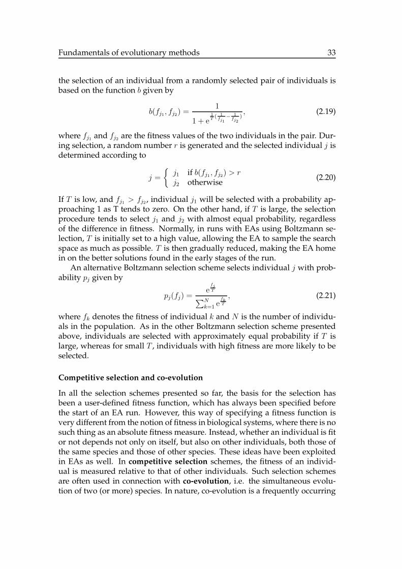
Fundamentals of evolutionary methods 33
the selection of an individual from a randomly selected pair of individuals isbased on the function b given by
b(fj1, fj2) =1
1 + e1T
( 1fj1
− 1fj2
), (2.19)
where fj1 and fj2 are the fitness values of the two individuals in the pair. Dur-ing selection, a random number r is generated and the selected individual j isdetermined according to
j =
{
j1 if b(fj1 , fj2) > rj2 otherwise
(2.20)
If T is low, and fj1 > fj2 , individual j1 will be selected with a probability ap-proaching 1 as T tends to zero. On the other hand, if T is large, the selectionprocedure tends to select j1 and j2 with almost equal probability, regardlessof the difference in fitness. Normally, in runs with EAs using Boltzmann se-lection, T is initially set to a high value, allowing the EA to sample the searchspace as much as possible. T is then gradually reduced, making the EA homein on the better solutions found in the early stages of the run.
An alternative Boltzmann selection scheme selects individual j with prob-ability pj given by
pj(fj) =e
fjT
∑N
k=1 efkT
, (2.21)
where fk denotes the fitness of individual k and N is the number of individu-als in the population. As in the other Boltzmann selection scheme presentedabove, individuals are selected with approximately equal probability if T islarge, whereas for small T , individuals with high fitness are more likely to beselected.
Competitive selection and co-evolution
In all the selection schemes presented so far, the basis for the selection hasbeen a user-defined fitness function, which has always been specified beforethe start of an EA run. However, this way of specifying a fitness function isvery different from the notion of fitness in biological systems, where there is nosuch thing as an absolute fitness measure. Instead, whether an individual is fitor not depends not only on itself, but also on other individuals, both those ofthe same species and those of other species. These ideas have been exploitedin EAs as well. In competitive selection schemes, the fitness of an individ-ual is measured relative to that of other individuals. Such selection schemesare often used in connection with co-evolution, i.e. the simultaneous evolu-tion of two (or more) species. In nature, co-evolution is a frequently occurring

Fundamentals of evolutionary methods 34
phenomenon. For example, predators may grow sharper fangs as a result ofthicker skin in their prey (and the prey, in turn, will then grow even thickerskin etc.).
In EAs, co-evolution is often implemented by considering two populations,where the fitness of the members of the first population is obtained from inter-actions with the members of the second population, and vice versa. A specificexample are the sorting networks evolved by Hillis [49]. In this application,the goal was to find sorting networks of order n, i.e. networks that can sortany permutation of the number 1, 2, . . . , n. In his experiments, Hillis used onepopulation of sorting networks, which was evolved against a population ofsequences to be sorted. The fitness of the sorting networks was measured bytheir ability to sort test sequences, and the fitness of the test sequences wasmeasured by their ability to fool the sorting networks, i.e. to make them sortincorrectly.
A problem with co-evolution is the issue of measuring absolute improve-ments, given that the fitness measure is a relative one. This problem can beattacked in various ways. A simple procedure (used e.g. by Wahde and Nor-dahl [132] in their work on pursuit and evasion in artificial creatures) is tomeasure the performance of the best individual (a pursuer, say, in the applica-tion considered in [132]) against a given, fixed individual. However, such anindividual cannot easily be defined in all applications.
Co-evolution is an interesting (and biologically motivated) idea, but it isnot applicable to all problems. In addition, the problems involved in measur-ing co-evolutionary progress (as discussed above) have made the use of co-evolution in EAs quite rare. However, there are some applications involvingER, and some references to those are given in Sect. 3.4.
2.7.4 Fitness measures
In many problems, e.g. function optimization, it is relatively easy to specifya fitness measure. However, in other problems, it is much more difficult. Anexample can be taken from the ER. Consider the problem of evolving a gait (i.e.a means of walking) for a simple model of a bipedal robot, namely the five-linkrobot shown in Fig. 3.24 in Subsect. 3.4.1 below, using, say, a neural network asthe brain of the robot. An obvious choice of fitness measure for this problem issimply the distance walked in a given amount of time, i.e. the position of thecenter-of-mass (COM) of the robot, at the end of an evaluation. However, withthis fitness measure it is usually found that the robot will throw itself forward,thus terminating the evalution, but at least reaching further than robots thatsimply collapse. Here, the problem stems from the fact that the step from arandom neural network to one that can generate the cyclical pattern neededfor legged locomotion is a very large one. Indeed, evolving a gait (for a pre-
Fundamentals of evolutionary methods 35
defined body shape) from random initial conditions is a very complex task,and the EA therefore takes the easier route of just throwing the body of therobot forward. Of course, if the EA did find an actual gait, however bad, thatcould keep the robot upright while walking slowly forward, the correspondingindividual would obtain a higher fitness value. However, such an individualis unlikely to be present in the early generations of the EA. In this particularcase, the problem can be solved by combining several criteria. For example,the fitness measure can be taken as a combination of the position of the feet andthe posture (e.g. the vertical position of the COM) at the end of the evaluation.
Furthermore, in ER, it is common that each individual must be evaluatedin a variety of situations, to prevent the EA from finding solutions that onlyperform well in certain specialized situations. Thus, in such cases, the robotshould be evaluated in a variety of different situations, and each evaluationwill result in a partial fitness value. Thus, when a robot has been completelyevaluated, there will be a vector of partial fitness values, from which a scalarfitness value must be obtained. Procedures for doing so will be given in Sect. 3.2.
Other complicated situations are those in which the fitness measure shouldtake into account several, possibly conflicting, criteria (multiobjective opti-mization). Another example is constrained optimization where not all possi-ble solutions are valid. Constrained optimization will not be considered fur-ther in this tutorial. The interested reader is referred to [84]. Multi-objectiveoptimization will, at least implicitly, be considered in some of the examples inChapter 3.
2.7.5 Alternative schemes for reproduction and replacement
In nature, there are restrictions on mating, the most obvious one being thatindividuals of one species generally do not mate with individuals of anotherspecies. However, mating restrictions exist even within species, as a result of,for example, geographical separation between individuals. In addition, to pre-vent inbreeding, biological organisms are designed to avoid mating with closerelatives. The concept of mating restriction has been exploited in EAs as well,and some brief examples will now be given. For a more detailed discussion,see e.g. [4].
Species-based EAs
In biology, one introduces the notion of species, to classify animals (and plants).Members of the same animal species are simply those that can mate3 and haveoffspring, or more correctly fertile offspring4. Speciation, i.e. the generation of
3For species that reproduce asexually, this definition can obviously not be used.4For example, a female tiger and a male lion (or vice versa) can have offspring (called a
liger), but the offspring is sterile.

Fundamentals of evolutionary methods 36
new species, occurs frequently in nature, often as a result of physical separa-tion (allopatry) of groups of individuals belonging to the same species. Aftermany generations, the descendants of those individuals may have evolved tobecome so different (genetically) that members from one group can no longerbreed with members of the other group, should they meet. This is so, sinceevolution will fine-tune animals (i.e. their genomes) to prevailing conditions.In addition, random accidents such as mutations, occur during recombinationof chromosomes and, if beneficial, such accidental changes may spread rapidlyin a population, thus making it genetically different from another populationin which the same random change has not taken place. In addition to mu-tations, gene duplication may also take place: It is common to find severalcopies of the same gene in a genome. In fact, it is believed [22] that at least twocomplete genome duplications have occurred in early vertebrates. Evidence forthis quadrupling of the genome can be obtained from studying a complex ofgenes known as hox5. The hox gene complexes are a set of transcription factorswhich are active during development of an animal, and which are responsiblefor determining the identity of different regions of a body, i.e. whether a partis to become a limb or something else. In many vertebrates (e.g. mammals),there are four hox gene complexes, suggesting that two genome duplicationshave occurred. Some EAs also use the concept of species. In such EAs, indi-viduals are only allowed to mate with individuals that share some properties,either on the genotype level or on the phenotype level. One of the simplestspeciation schemes is to allow crossover only between individuals for whichthe Hamming distance of the chromosomes, defined as the number of genesfor which the two chromosomes have different alleles (assuming a binary rep-resentation), does not exceed a pre-specified maximum value D.
In other EAs, the properties of the objects being optimized may provide anatural basis for mating restriction. For example, in the optimization of ANNs,a simple mating restriction procedure is to allow crossover only between indi-viduals with identical structure.
In general, one of the main ideas behind the introduction of species is toavoid matings of very different individuals, since such matings often result inrather bad individuals, especially when the EA has been running for a whileso that the parents have already started approaching (local) optima.
2.7.6 Subpopulation-based EAs
In subpopulation-based EAs, the population of N individuals is divided intoNs groups with ν = N/Ns individuals each. Mating is only allowed to take
5The hox genes belong to a larger family of genes called homeobox genes. Mutations tohomeobox genes can cause visible phenotypic changes. An example is the fruit fly DrosophilaMelanogaster, in which an extra set of legs may be placed in the position normally occupiedby antennae in the, a result of mutations in homeobox genes

Fundamentals of evolutionary methods 37
A
Figure 2.13: Premature convergence in an EA. In the original population, shown in the leftpanel, one individual (marked A) has significantly higher fitness than the others. Thus, thegenetic material of individual A will spread rapidly in the population, normally resulting inthe situation shown in the right panel: Convergence to a local optimum.
Figure 2.14: Mating restriction in a grid-based EA. The selected individual, representedby the dark, central square in the figure, is only allowed to mate with one of its immediateneighbors, shown as white squares.
place between individuals in the same subpopulation. Such EAs are also calledisland models, for obvious reasons. The idea behind subpopulation-basedEAs is to prevent situations in which an EA rapidly converges towards a localoptimum (a situation known as premature convergence), making it difficultto reach the global optimum, as illustrated in Fig. 2.13. In a subpopulation-based EA, it is less likely that, in the initial generation, all the best individualsin the subpopulations are located close to the same local optimum. Thus, inlater generations, when a certain amount of convergence inevitably occurs, itis more likely to find an individual reaching the global maximum rather thana local one.
However, if no interaction is allowed between individuals of different sub-populations, a subpopulation-based EA simply amount to running Ns EAswith ν individuals each. Thus, tunneling is allowed with some small probabil-

Fundamentals of evolutionary methods 38
ity pt. Tunneling can be achieved simply by swapping two indiviuals betweensubpopulations.
2.7.7 Grid-based EAs
In grid-based EAs, individuals are placed in a regular pattern as shown inFig. 2.14, and mating restrictions are introduced based on the placement ofindividuals on the grid. When an individual i on the grid is to be replaced bya new individual, parents are selected only in the neighborhood of the indi-vidual i. In the figure, the neighborhood contains eight individuals, but otherneighborhood sizes are, of course, possible as well.
The topology of the grid can be chosen in many different ways. A commonprocedure is to use periodic boundary conditions, in which the two edges ofa rectangular grid are joined to form a toroidal space. Grid-based EAs are alsocalled diffusion models.
2.8 Related algorithms
In view of their simplicity and general applicability, EAs have been appliedsuccessfully in many different problems involving optimization. However,during the last decade or so, several other stochastic optimization algorithms,with roughly the same applicability as EAs, have entered the stage. Two suchmethods are ant colony optimization (ACO) [26] and particle swarm opti-mization (PSO) [62]. Like EAs, both algorithms are population-based, i.e. alarge number of candidate solutions to the problem at hand are maintained.In addition, both algorithms are biologically inspired: ACO is based on theforaging behavior of ants, whereas PSO is based on the flocking behavior ofbirds (or, equivalently, the schooling behavior of fish).
During foraging, ants communicate by means of pheromones, a chemicalsubstance that indicates the recent presence of an ant. When an ant discoversa food source and then returns to the nest, other ants will be able to follow itspheromone trail to the same food source, thus further increasing the amountof pheromone along the trail. ACO operates essentially in the same way, usingartificial pheromones. A typical application is the traveling salesman prob-lem, where the objective is to find the shortest path visiting N cities (or nodesin a network) once and only once. In order to solve the problem, a group ofartificial ants is released and given the task of moving between the N cities,depositing artificial pheromone as they go, and also selecting their moves de-pending on the level of artificial pheromone that they encounter. Once allants have completed their task, a new group of ants is released etc. The levelof pheromone deposited by an ant is then taken essentially inversely propor-tional to the length of the corresponding path, making this path a more likely
Evolutionary robotics 39
choice than a longer path for the next set of ants.ACO is commonly more efficient than EAs on the traveling salesman prob-
lem. However, not all problems can easily be formulated in a way suitable forACO. By contrast, PSO can be applied to any problem that EAs can solve. InPSO, a population of candidate solutions (referred to as particles) is generated,just as in an EA. In addition to keeping track of the position (x1, x2, . . . , xK)of a given particle in the K−dimensional search space (just as one would doin an EA, where the position would be defined by the variables decoded fromthe chromosome of the individual), each particle is also given a velocity. Thus,rather than generating new individuals by crossover and (random) mutations,as in an EA, in PSO particles are moved (rather than replaced) by integratingtheir equations of motion. The acceleration of a given particle is determined by(1) the position of each particle in relation to the overall best position, i.e. theone associated with the highest value of the fitness function f(x1, x2, . . . , xK)(assuming maximization) found so far, and (2) the position of each particle inrelation to the previous best position of the particle itself. Thus, particles aredrawn towards regions of higher fitness, while still exploring other regions onthe way.
Even though both PSO and ACO are becoming increasingly popular inrobotics, it is so far EAs that have found most applications in the field of au-tonomous robots, and the remainder of this tutorial will be focused on theapplication of EAs in robotics.

Chapter 3
Evolutionary robotics
3.1 Introduction
In this chapter the main topic of this tutorial, namely the generation of roboticbodies and brains by means of EAs will be considered. This is a vast andrapidly growing area of research, and therefore, by necessity, only a few as-pects will be covered in detail in this tutorial. However, it is the author’s hopethat the topics covered with be representative of the field as a whole, and thatthe reference list at the end of the tutorial will provide useful directions forfurther reading.
ER has been applied in a large variety of different situations. Most appli-cations, however, can be considered part of the subfield of robotics known asbehavior-based robotics, and it is therefore appropriate to give a very briefintroduction to this topic. The reader is referred to [3], and references therein,for a more thorough introduction.
3.1.1 Behavior-based robotics
The concept of behavior-based robotics (BBR) was introduced in the mid 1980s,and was championed by Rodney Brooks [14] and others. BBR approaches in-telligence in a way that is very different from the classical AI approach, and aschematic illustration of the difference in given in Fig. 3.1. In classical artificialintelligence (AI), the flow of information is as shown in the left panel of thefigure. First, the sensors of the robot sense the environment. Next, a (usuallyvery complex) world model is built, and the robot reasons about the effectsof various actions within the framework of this world model, before finallydeciding upon an action, which is executed in the real world.
Now, this procedure, shown in the left panel of Fig. 3.1, is very differentfrom the distributed form of computation found in the brains of biological or-ganisms, and, above all, it is generally very slow, strongly reducing its survival
40
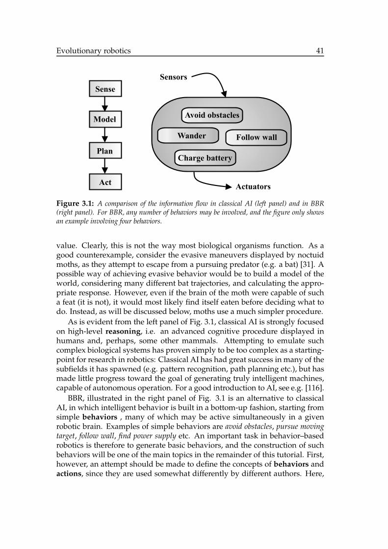
Evolutionary robotics 41
Sense
Plan
Act
ModelAvoid obstacles
Follow wall
Charge battery
Wander
Sensors
Actuators
Figure 3.1: A comparison of the information flow in classical AI (left panel) and in BBR(right panel). For BBR, any number of behaviors may be involved, and the figure only showsan example involving four behaviors.
value. Clearly, this is not the way most biological organisms function. As agood counterexample, consider the evasive maneuvers displayed by noctuidmoths, as they attempt to escape from a pursuing predator (e.g. a bat) [31]. Apossible way of achieving evasive behavior would be to build a model of theworld, considering many different bat trajectories, and calculating the appro-priate response. However, even if the brain of the moth were capable of sucha feat (it is not), it would most likely find itself eaten before deciding what todo. Instead, as will be discussed below, moths use a much simpler procedure.
As is evident from the left panel of Fig. 3.1, classical AI is strongly focusedon high-level reasoning, i.e. an advanced cognitive procedure displayed inhumans and, perhaps, some other mammals. Attempting to emulate suchcomplex biological systems has proven simply to be too complex as a starting-point for research in robotics: Classical AI has had great success in many of thesubfields it has spawned (e.g. pattern recognition, path planning etc.), but hasmade little progress toward the goal of generating truly intelligent machines,capable of autonomous operation. For a good introduction to AI, see e.g. [116].
BBR, illustrated in the right panel of Fig. 3.1 is an alternative to classicalAI, in which intelligent behavior is built in a bottom-up fashion, starting fromsimple behaviors , many of which may be active simultaneously in a givenrobotic brain. Examples of simple behaviors are avoid obstacles, pursue movingtarget, follow wall, find power supply etc. An important task in behavior–basedrobotics is therefore to generate basic behaviors, and the construction of suchbehaviors will be one of the main topics in the remainder of this tutorial. First,however, an attempt should be made to define the concepts of behaviors andactions, since they are used somewhat differently by different authors. Here,
Evolutionary robotics 42
a behavior will be defined simply as a sequence of actions performed in orderto achieve some goal. Thus, for example, an obstacle avoidance behavior mayconsist of the actions of stopping, turning, and starting to move again. Note,however, that the definition is not very strict, and that the terms behavior andaction remain somewhat blurred.
Returning to the example of the moth, its evasive behavior is very simpleindeed, and is in fact based on only a few neurons and an ingenious position-ing of the ears on its body. This simple system enables the moth to fly awayfrom an approaching bat and, if it is unable to shake off the pursuer, start tofly erratically to confuse the predator [31].
The example with the moth shows that intelligent behavior does not re-quire reasoning1, and in BBR one generally uses a more generous definition ofintelligent behavior than that implicity used in AI. Thus, in BBR, one may de-fine intelligent behavior as the ability to survive, and to strive to reach other goals,in an unstructured environment. This definition is more in tune with the fact thatmost biological organisms are capable of highly intelligent behavior in the en-vironment for which they have been designed, even though they may fail quitebadly in novel environments (as illustrated by the failure of e.g. a fly caught infront of a window). As mentioned in Chapter 1, an unstructured environmentis an environment that changes rapidly and unexpectedly, so that it is impossi-ble to rely on pre–defined maps, something that holds true for most real-worldenvironment. For example, if it is the task of a robot to transport equipment ina hospital, it must first be able to avoid (moving) obstacles. Putting a completeplan of the hospital into the robot will not be sufficient, since the environmentchanges on a continuous basis. The robot may pass an empty room, only tofind the room full of people or equipment when it returns.
Different behavior-based robots generally share certain features, even thoughnot all features are present in all such robots. To start with, behavior-basedrobots are first provided with the most basic behaviors such as obstacle avoid-ance or battery charging, needed to function in an unstructured environment.More complex behaviors are added at a later stage. Secondly, several behav-iors are generally in operation simultaneously, and the final action taken bythe robot represents either a choice between the suggestions given by the var-ious behaviors, or an average action formed from the actions suggested byseveral behaviors. Thirdly, BBR is mostly concerned with autonomous robots,i.e. robots that are able to move freely and without direct human supervision.Finally, the concept of situatedness is a central tenet of BBR: Behavior-basedrobots do not build complex, abstract world models. Instead, they read theinformation available through their sensors, and take actions based on that in-formation. Thus, behavior-based robots are generally situated (i.e. operate inthe real world), and many behaviors in BBR are reactive [95], i.e. have a di-
1The concept of rational behavior will be considered in Subsect. 3.3.3.

Evolutionary robotics 43
rect coupling between sensors and actuators. However, internal states are ofcourse allowed and are often very useful, but, to the extent that such states areused, they are not in the form of abstract world models.
Note that, in ER, it is often necessary to use simulations rather than ac-tual robots. While the use of simulations represents a step away from the re-quirement of situatedness, the simulations used in BBR differ strongly fromthe construction of abstract world models: Just as in a real, behavior-basedrobot, a simulated robot in BBR will rely only on the information it can gatherthrough its simulated sensors, and the reading of a sensor, in itself, never pro-vides explicit information about e.g. the distance to a detected object.
Clearly, no simulation can capture all the facets of reality. Thus, it is impor-tant to test, in real robots, any results obtained through simulations. The issueof evolution in simulations versus evolution in hardware will be consideredbriefly in Subsect. 3.4.2.
In general, the construction of a complete brain for a behavior-based robotcan be considered a two-stage process: First the individual behaviors must bedefined (or evolved, in the case or ER). Next, a system for selecting which ac-tion to take, based on the suggestions available from the individual behaviors,must be constructed as well. Clearly, in any robot intended for complex appli-cations, the behavioral selection system is just as important as the individualbehaviors themselves. For example, returning to the example of the hospitalrobot, it is clear that if it starts to run out of power, it must reprioritize its goalsand quickly try to find a power supply, even if, by doing so, it comes no closerto achieving its task of delivering objects. Methods for Behavioral organiza-tion, (also called action selection, behavioral coordination, and behavioralselection) have been the subject of much research in BBR. While a completesurvey of such methods is beyond the scope of this text, a few methods for be-havioral selection based on evolutionary algorithms will be considered belowin Sect. 3.3. For a review of methods for behavioral organization, see e.g. [108].Other relevant references on this topic are e.g. [9], [78], and [131].
3.1.2 Evolving robots
The aim of ER is to use EAs to evolve robotic brains2 (or bodies, or both),rather than designing them by other means, e.g. by hand. There are manyreasons for using artificial evolution to generate robotic brains [46], [47], oneof the most important being that it is very difficult to design such systems byhand in any but the simplest cases. In a non-controlled setting, i.e. any real-istic environment, there will always be many sources of noise, as well as both
2As mentioned in Chapter 1, in this tutorial, the term robotic brain will be used instead ofthe term control system, since the latter term is indicative of the more limited types of systemsconsidered in classical control theory.

Evolutionary robotics 44
stationary and moving obstacles and, perhaps, other robots as well. Trying topredict which situations may occur in such an environment is a daunting task,and hand-coded robotic brains are therefore generally non-robust and proneto failure. On the other hand, properly evolved robotic brains, i.e. those gener-ated using either physical robots or simulations involving realistic noise at alllevels, are often able to cope quite well with their environment, even though, infairness, it should be mentioned that the robotic brains evolved so far are quitesimple compared to the ultimate goal of truly intelligent machines. However,the complexity of evolved robotic brains is steadily increasing, and EAs arenow used not only for constructing simple behaviors, but also for generatingcomplex systems for behavioral organization [107], [131].
Furthermore, evolution (whether natural or artificial) is often able to findsolutions that are remarkably simple, yet difficult to achieve by other means.
Another advantage with EAs in connection with robots, is that their abil-ity to function even with very limited feedback. This is important in robotics,where it is often known what a robot should do, but perhaps not how it shoulddo it, e.g. in what order different behaviors should be activated, at what pointa task should be suspended in order to engage in self-preserving activities suchas obstacle avoidance etc. In other words, it is difficult to specify directly theadequacy of any single action: Feedback is often obtained long after an actionis performed, resulting in a credit assignment problem, i.e. the problem ofassigning credit (or blame) to previous actions. EAs are very well suited tothis kind of problems, where only rather vague guidance can be given. Anexample is the evolution of the simple cleaning behavior presented in Chap-ter 1: The simulated evolving robots were not told first to approach objects,then start pushing them, correcting the heading when needed etc. Instead, theonly feedback available was the final state, and the intermediate steps werethe result of evolution.
Of course, as with all methods, there are also some drawbacks with ER, oneof the most serious being that, in view of the many candidate robotic brainsthat must be examined before a satisfactory one is found, it is usually requiredto resort to the use of simulations, rather than evolving in actual, physicalrobots. Making realistic simulations is indeed difficult, and there exists a re-ality gap [59] between simulated and physical robots. However, as will bediscussed in Subsect. 3.4.2 below, it is possible to overcome the reality gap,and the need for using simulations does not, in fact, introduce fundamentallimits on the results obtained from ER.
In the remainder of this chapter, several examples of ER will be given, alongwith a discussion of several general issues that appear in most ER applications.The flow of an ER investigation is shown in Fig. 3.2, and it is quite similar tothe flow of a general EA. The figure is simplified: The procedure of formingindividuals can involve anything from setting a few parameters to runninga complex developmental process (see Subsect. 3.4.3 below), generating both

Evolutionary robotics 45
Evaluate inphysical robot
Form individual
Assign fitness
Arena
Allindividualsevaluated?
No
Initialize population
Yes
Generate new population
Satisfactoryresult obtained?
No
YesTerminate run
Validate results inphysical robots
Physics
Evaluate insimulation
Figure 3.2: The flow of an ER investigation. Note that some steps, e.g. formation of individ-uals and new populations, are shown in a strongly simplified way.
the brain and the body of a robot. The dashed arrows in the figure indicate achoice: As mentioned above, in many ER investigations, simulations are usedand, as indicated in the figure, the evaluation of an individual requires simu-lating the physics of the arena in which the evaluation takes place. The otheroption is to use actual, physical robots, and, in this case, the most commonapproach is to generate individuals in a computer, upload them one by oneon a single robot, evaluate the robot, and return its fitness. There are otherapproaches as well (not shown in the figure), such as embodied evolution[33], [140], where the entire evolutionary process takes place on a populationof physical robots. Incidentally, if evolution is carried out in physical robotsaccording to the scheme shown in Fig. 3.2, some restrictions are placed on thefitness measure, since it must be possible for the robot to assess its fitness andreturn the result to the computer, at least in cases where the EA is to operatewithout continuous human supervision. Thus, the fitness measure must bebased on quantities that are readily available to the robot, such as e.g. sensorsreadings, motor speeds etc. [34].
The final step in Fig. 3.2, i.e. the validation of the results in physical robots,is perhaps the most important step. A robotic brain that only functions insimulation is of little use. Note that validation should be carried out even ifthe evolution has been performed using a single physical robot. This is so,since all physical robots have individual characteristics. For example, there is

Evolutionary robotics 46
Figure 3.3: A schematic illustration of a differentially steered robot, equipped with threesensors. The wheels, shown as rectangles, are independently controlled. The vertical lineindicates the direction of motion (for positive wheel speeds).
no such thing as two completely identical IR sensors, even if they come fromthe same manufacturer and have the same product number.
If the validation does not give satisfactory results, there are two differentoptions, either to extend the EA run, or to attempt to adjust the robotic brain(or body) by hand. A useful approach in extended runs may be to switch fromsimulations to physical robots. Even a short extended run may then lead toimproved results [86].
The architectures used for robotic brains can be chosen in a variety of ways.It is common to use ANNs (see Appendix A), but other architectures are usedas well, as will be discussed below.
Robots used in ER investigations are of many kinds, including walkingrobots (see Subsect. 3.4.1) and wheeled robots. A common type of wheeledrobot for ER is the Khepera robot (see Appendix C), for which there also existsseveral simulators (see Subsect. 3.4.4). In general, differentially steered robots,such as Khepera, are also simple to model and thus to use in simulations. Thebasic equations of motion for such robots can be taken as
Mv + αv = A (τL + τR) , (3.1)
andIϕ+ βϕ = B (−τL + τR) , (3.2)
where M is the mass of the robot, I its moment of inertia (with respect tothe vertial axis), v its speed, and ϕ its direction of motion. τL and τR are thetorques acting on the left and right wheels, respectively. A and B are constantsdepending on geometrical and physical factors (such as the radius and mass
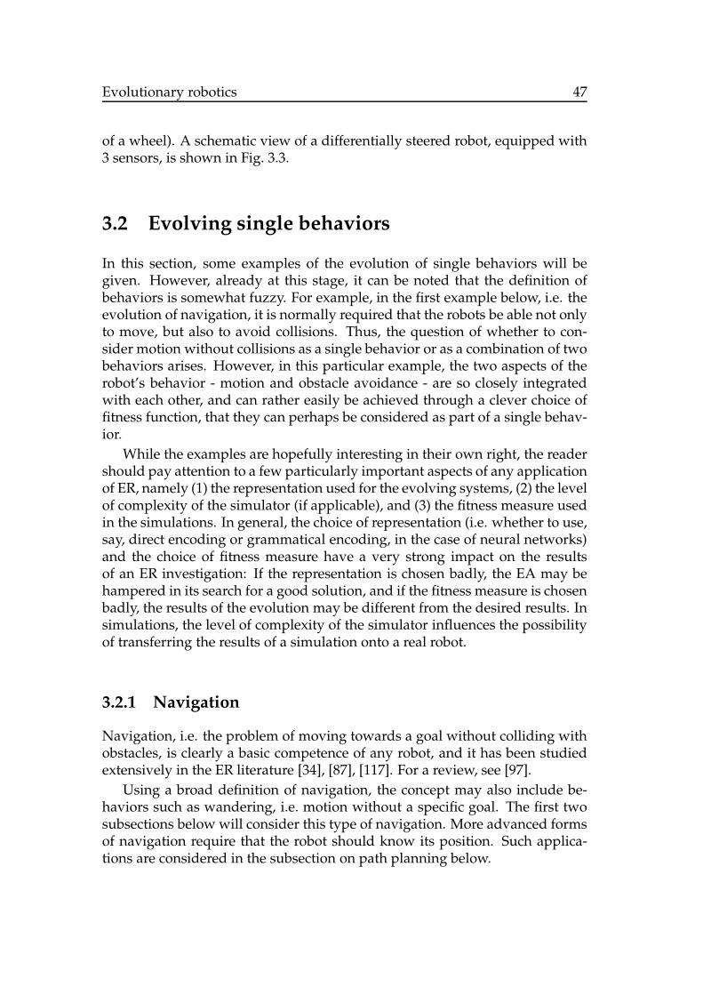
Evolutionary robotics 47
of a wheel). A schematic view of a differentially steered robot, equipped with3 sensors, is shown in Fig. 3.3.
3.2 Evolving single behaviors
In this section, some examples of the evolution of single behaviors will begiven. However, already at this stage, it can be noted that the definition ofbehaviors is somewhat fuzzy. For example, in the first example below, i.e. theevolution of navigation, it is normally required that the robots be able not onlyto move, but also to avoid collisions. Thus, the question of whether to con-sider motion without collisions as a single behavior or as a combination of twobehaviors arises. However, in this particular example, the two aspects of therobot’s behavior - motion and obstacle avoidance - are so closely integratedwith each other, and can rather easily be achieved through a clever choice offitness function, that they can perhaps be considered as part of a single behav-ior.
While the examples are hopefully interesting in their own right, the readershould pay attention to a few particularly important aspects of any applicationof ER, namely (1) the representation used for the evolving systems, (2) the levelof complexity of the simulator (if applicable), and (3) the fitness measure usedin the simulations. In general, the choice of representation (i.e. whether to use,say, direct encoding or grammatical encoding, in the case of neural networks)and the choice of fitness measure have a very strong impact on the resultsof an ER investigation: If the representation is chosen badly, the EA may behampered in its search for a good solution, and if the fitness measure is chosenbadly, the results of the evolution may be different from the desired results. Insimulations, the level of complexity of the simulator influences the possibilityof transferring the results of a simulation onto a real robot.
3.2.1 Navigation
Navigation, i.e. the problem of moving towards a goal without colliding withobstacles, is clearly a basic competence of any robot, and it has been studiedextensively in the ER literature [34], [87], [117]. For a review, see [97].
Using a broad definition of navigation, the concept may also include be-haviors such as wandering, i.e. motion without a specific goal. The first twosubsections below will consider this type of navigation. More advanced formsof navigation require that the robot should know its position. Such applica-tions are considered in the subsection on path planning below.

Evolutionary robotics 48
Figure 3.4: The environment used in the evolution of navigation in [34]. Reproduced withkind permission of Dr. D. Floreano.
Basic navigation
In [34], Floreano and Mondada evolved basic navigation. The authors specif-ically pointed out the difficulties in constructing accurate simulations, andchose instead to evolve navigation behavior in a real Khepera robot (see Ap-pendix C). The aim was to evolve collision-free navigation in an environmentwith stationary obstacles, shown in Fig. 3.4. In the experiments, the authorsused a simple, fixed-length chromosome to encode the weights of neural net-works of fixed structure. The networks consisted of a single layer of synapticweights, connecting the 8 IR sensors of the Khepera robot to two output neu-rons, connected to the motors. In addition, recurrent connections were intro-duced within the output layer.
The fitness contribution for each time step during the motion of the robotwas chosen as
Φ = V(
1 −√
|∆v|)
(1 − i), (3.3)
where V denotes the average rotation speed of the wheels, ∆v is the differencebetween the (signed) speeds of the wheels, and i is the value of the IR sen-sor with the highest reading. V , |∆v|, and i were all normalized to the range[0, 1], so that Φ also was constrained to this range. The complete fitness func-tion f was obtained by summing the values of Φ obtained for each time step,and then dividing the results by the number of time steps. The same fitnessmeasure was used also by Nolfi et al. [99].
The first factor (V ) in Eq. (3.3) promotes high speed, whereas the second
factor, 1 −√
|∆V |, promotes straight-line motion, and the third factor (1 − i)rewards obstacle avoidance. Note that the different factors in the fitness mea-sure counteract each other, to some extent. For example, the environment wassuch that the robot was required to turn quite often in order to avoid colli-sions, even though the second factor in the fitness measure would discourageit to do so. This is an example of what could be called an explicit fitness mea-sure, since explicit punishments (in the form of a reduced increase in fitness)are given if the speed is low, if the robot does not move in a straight line, or if

Evolutionary robotics 49
Figure 3.5: The maze used by Nelson et al. [92] for the evolution of navigation, reproducedwith kind permission of the authors. The figure shows some results obtained in simulation.Qualitatively similar results were obtained using a physical robot, EvBot, shown in Fig. 3.6.
the robot approaches an obstacle. The alternative is to use an implicit fitnessmeasure for some of the aspects of the robot’s motion. For example, in [59],Jakobi et al. used a fitness measure similar to the one given in Eq. (3.3), butwithout the factor (1 − i), since it was found that this factor is unnecessary ina sufficiently cluttered environment, where obstacle avoidance is an implicitrequirement for any form of motion.
Floreano and Mondada report that the best evolved robots successfullynavigated through their environment, and that some robots also showed in-telligent behavior beyond what was explicitly encoded in the fitness function.For example, some of the best robots learned to modulate the speed, keepingit at around three quarters of the maximum allowed speed in the vicinity ofobstacles.
While evolving robotic behaviors in hardware has obvious advantages, apossible disadvantage is that it is often quite time-consuming. Indeed, in theexperiments reported in [34], each generation lasted around 40 minutes. Inorder to evolve successful robots, around 50-100 generations were needed.
In addition to basic navigation, Floreano and Mondada also evolved hom-ing navigation, in which the robot was required periodically to recharge its(simulated) batteries. However, this was a more complex task, and it will beconsidered briefly in the discussion on complex behaviors and behavioral or-ganization in Sect. 3.3 below.
While some recurrent connections were included in the output layer of theneural networks used in [34], Nelson et al. [92] made more explicit use of tem-poral processing of information, motivated by the fact that robots commonlyshow suboptimal performance using reactive behaviors based on very poorsensory inputs.
Thus, Nelson et al. considered neural networks with several layers con-taining recurrent couplings as well as time-delayed couplings. The neural net-works were evolved in simulations involving robots equipped with 5 simple

Evolutionary robotics 50
Figure 3.6: The EvBot robot used in [92]. The robot is equipped with an array of tactilesensors, and can also be fitted with other sensors, such as video cameras. Reproduced withkind permission of Nelson et al.
tactile sensors. The task of the simulated robots was to navigate in a maze,shown in Fig. 3.5. The fitness measure was taken essentially as the distancetravelled, with a penalty for situations in which the robot became stuck.
It was indeed found that robots equipped with memory, in the form ofrecurrent couplings and time-delay elements, performed the navigation taskbetter than purely reactive robots. The best results were obtained for networksof moderate complexity, containing 1-3 hidden layers with 5-10 neurons perlayer. The best networks obtained during evolution were transferred, withretained functionality, to an actual robot (EvBot, shown in Fig. 3.6), equippedwith five tactile sensors.
Wandering behavior
Miglino et al. [87] evolved an exploratory behavior (also called wandering) insimulations. The resulting behaviors were then tested in actual (Lego) robots.In this case, the brains of the robots were represented by very simple neuralnetworks, with two inputs from a front sensor and a rear sensor, two hiddenunits, and two outputs controlling the two motors. In addition, a single mem-ory neuron was used, connecting the hidden layer to itself through a recurrentcoupling. All signals were binary (a Heaviside step function was used as thethreshold function in the neurons), and the simple neural networks used inthis study could, in fact, be represented as finite-state machines (see AppendixB).
In order to achieve wandering behavior, the authors used a fitness measurewhich rewarded movements that would take the robot to locations where ithad not been before. The robot was placed in an arena of size 2.6× 2.6 meters,

Evolutionary robotics 51
consisting of squares with 0.10 m side length. The central 20 × 20 square hadwhite color, and the remaining squares were black, so that the robot coulddetermine whether or not it was close to a boundary.
The fitness of the evolving robotic brains was incremented by one everytime the robot visited a square it had not previously visited, and the final fit-ness measure was taken as the fraction of squares visited.
An important issue in ER is the fact that an EA will try to exploit the par-ticularities of the encountered situations as much as possible. Thus, in theevolution of wandering behavior, if a single starting position was used in allevaluations, the EA would quickly find a way to optimize the motion of therobot based on the given starting position. In order to avoid such problems,Miglino et al. evaluated each robotic brain 10 times, starting from a randomlocation in the grid.
The authors report that the best evolved robotic brains managed to makethe corresponding robot visit an average of slightly more than half of the avail-able squares. The evolutionary process exhibited three clear stages, duringwhich the maximum fitness was essentially constant. The stages correspondedto different levels of complexity. For example, in the first stage, the evolvedneural networks made no use of the memory unit, whereas in the second stagethey did.
The neural networks obtained in the simulations where then implementedin actual Lego robots. While the behaviors of the actual robots were similar tothose of the simulated ones, there were some clear differences, some of whichwere attributed to noise (absent in the simulations). Thus, some simulationswere made with noise added, and it was found that a closer correspondencebetween the behavior of real robots and simulated robots could be found if thelatter were evolved at intermediate levels of noise.
Path planning
Path planning, the problem of determining the optimal route from a startingposition to a goal position, has been studied extensively in robotics in gen-eral, and also, to some extent, within the field of ER. A basic requirementfor path planning is localization, i.e. knowledge of one’s position. In manyER-related path planning studies, it is simply assumed that the localizationproblem has been solved, and the investigation instead centers on the prob-lem of finding suitable paths that avoid collisions with obstacles. However,some authors have considered the problem of localization. For example, Duck-ett [27] describes an EA-based method for simultaneous localization and map-ping (SLAM) and Pettersson et al. [105] recently developed a localization al-gorithm based on odometry, where the duration of execution of the behaviorfor odometry calibration (based on laser range finder scan matching) is es-sentially determined by an EA. With the assumption of sufficiently accurate
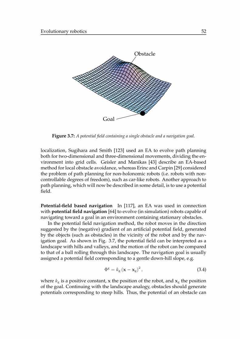
Evolutionary robotics 52
Obstacle
Goal
Figure 3.7: A potential field containing a single obstacle and a navigation goal.
localization, Sugihara and Smith [123] used an EA to evolve path planningboth for two-dimensional and three-dimensional movements, dividing the en-vironment into grid cells. Geisler and Manikas [43] describe an EA-basedmethod for local obstacle avoidance, whereas Erinc and Carpin [29] consideredthe problem of path planning for non-holonomic robots (i.e. robots with non-controllable degrees of freedom), such as car-like robots. Another approach topath planning, which will now be described in some detail, is to use a potentialfield.
Potential-field based navigation In [117], an EA was used in connectionwith potential field navigation [64] to evolve (in simulation) robots capable ofnavigating toward a goal in an environment containing stationary obstacles.
In the potential field navigation method, the robot moves in the directionsuggested by the (negative) gradient of an artificial potential field, generatedby the objects (such as obstacles) in the vicinity of the robot and by the nav-igation goal. As shown in Fig. 3.7, the potential field can be interpreted as alandscape with hills and valleys, and the motion of the robot can be comparedto that of a ball rolling through this landscape. The navigation goal is usuallyassigned a potential field corresponding to a gentle down-hill slope, e.g.
Φg = kg (x − xg)2 , (3.4)
where kg is a positive constant, x the position of the robot, and xg the positionof the goal. Continuing with the landscape analogy, obstacles should generatepotentials corresponding to steep hills. Thus, the potential of an obstacle can
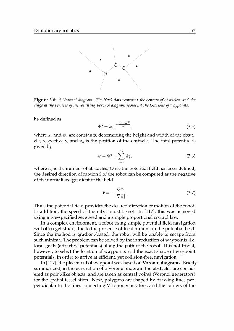
Evolutionary robotics 53
VL VRp1w1
w0
w1
w1p
u2p1
w2 p5
p4p2
u1
w3
Figure 3.8: A Voronoi diagram. The black dots represent the centers of obstacles, and therings at the vertices of the resulting Voronoi diagram represent the locations of waypoints.
be defined as
Φo = koe−
(x−xo)2
w2o , (3.5)
where ko and wo are constants, determining the height and width of the obsta-cle, respectively, and xo is the position of the obstacle. The total potential isgiven by
Φ = Φg +
no∑
i=1
Φoi , (3.6)
where no is the number of obstacles. Once the potential field has been defined,the desired direction of motion r of the robot can be computed as the negativeof the normalized gradient of the field
r = − ∇Φ
|∇Φ| . (3.7)
Thus, the potential field provides the desired direction of motion of the robot.In addition, the speed of the robot must be set. In [117], this was achievedusing a pre-specified set speed and a simple proportional control law.
In a complex environment, a robot using simple potential field navigationwill often get stuck, due to the presence of local minima in the potential field:Since the method is gradient-based, the robot will be unable to escape fromsuch minima. The problem can be solved by the introduction of waypoints, i.e.local goals (attractive potentials) along the path of the robot. It is not trivial,however, to select the location of waypoints and the exact shape of waypointpotentials, in order to arrive at efficient, yet collision-free, navigation.
In [117], the placement of waypoint was based on Voronoi diagrams. Brieflysummarized, in the generation of a Voronoi diagram the obstacles are consid-ered as point-like objects, and are taken as central points (Voronoi generators)for the spatial tessellation. Next, polygons are shaped by drawing lines per-pendicular to the lines connecting Voronoi generators, and the corners of the

Evolutionary robotics 54
resulting polygons are taken as the waypoint locations. The procedure is illus-trated in Fig. 3.8.
The potentials of the waypoints can be modelled e.g. as
Φp = kpe−
(x−xp)2
w2p , (3.8)
i.e. the same form as the obstacle potentials, but with negative constants kp.When the waypoints have been placed, and their potentials have been deter-mined, navigation proceeds as in standard potential field navigation, with thedirection of motion provided by the potential field, the only difference beingthat waypoints are successively removed as the robot passes in their vicinity toprevent it from being attracted back toward waypoints that have already beenpassed.
Once the location of obstacles in a given environment is known, the loca-tion of waypoints is generated deterministically through the procedure justdescribed. What remains to be determined is the depth (or height, in the caseof obstacles) of the potentials for the goal, obstacles, and waypoints, as wellas the widths of the potentials (i.e. wo for obstacles etc.). In [117], the authorsused an EA to determine suitable values for these parameters. In addition, thereference speed used in the proportional control law was determined by theEA. In fact, two reference speeds were used, v1
ref (for general navigation) andv0ref (near obstacles). Furthermore, the EA determined the distance do from the
closest obstacle at which a simulated robot would lower its set speed from v1ref
to v0ref , as well as the distance dw (between a waypoint and the robot) at which
the waypoint was removed.Thus, in all, a total of 10 parameters had to be determined, and, for this
purpose, the authors used a standard genetic algorithm (GA) with tournamentselection, single-point crossover, and mutation.
As in the navigation of wandering behavior discussed above, the authorsevaluated each set of parameters several times, in order to avoid overfitting toany particular environment.
For each evaluation, the fitness measure was calculated as
fi =Tmax
Te−
dD , (3.9)
where T denotes the time at which the robot reached the navigation goal, atwhich point the evaluation would be terminated. In addition, all evaluationshad a maximum duration of Tmax, whether or not the robot reached the goal.Furthermore, if the robot physically hit an obstacle, the evaluation was ter-minated immediately and T was set to Tmax. d denotes the distance betweenthe robot and the goal at termination, and D is the initial distance betweenthe robot and the goal. With this fitness measure, the robot was rewarded formoving quickly, and without collisions, toward the goal.
Evolutionary robotics 55
10.0s
Figure 3.9: The navigation of a simulated robot from [117] is shown in the left panel. Thesnapshot was taken after 10.0s in a simulation in which the goal was reached after 29.8s. In theright panel, a photograph of the actual Khepera II robot, navigating in the same environment,is shown. The robot, seen from above, is the smaller circle near the center of the photograph.
In all, 20 different environments, with different locations of obstacles, wereused in the evaluation of each individual (i.e. parameter set), and a final fitnessmeasure was formed by weighing the results of the Ne = 20 evaluations. Now,a common approach for doing so is to consider the average fitness, i.e.
f (1) =1
Ne
Ne∑
i=1
fi, (3.10)
The authors report that the runs with fitness measure f (1) achieved only medi-ocre results. This is understandable, as the fitness measure f (1) only measuresaverage performance, therefore making it possible for the simulated robot tofail completely in some environments and still achieve a rather high average.By contrast, fitness measure f (2)
f (2) = minifi, (3.11)
which was also used, focuses completely on the worst performance of therobot, and tends to generate results that are more robust. In fact, in all runswith this fitness measure, the simulated robot with the motion determined bythe best individual of the EA managed to reach its goal position in all environ-ments.
Next, the results from the simulations were transferred to an actual Khep-era II robot (see Appendix C). Clearly, the potential field navigation methodrequires accurate positioning, and it turned out that the drift in the devia-tion between actual and estimated position (based on dead reckoning) wastoo large if the dynamics of the robot was integrated as in the simulations.Thus, a simplified scheme was implemented, in which the robot navigated indiscrete steps. In each step the robot started from a standstill, determined (via
Evolutionary robotics 56
the potential field) its desired direction of heading, moved a distance δ in thisdirection, and stopped again. Provided that δ was chosen sufficiently small,this navigation procedure represents a slow-motion version of that used in thesimulations. Using this procedure, the Khepera robot rather successfully (butslowly) navigated through one of the most difficult environments used in thesimulations. Snapshots of a simulated robot and a physical robot navigatingin this environment are shown in Fig. 3.9.
3.2.2 Box-pushing
Simple Box-pushing can be used as a metaphor for behaviors needed, for in-stance, in transportation robots, and it has been investigated by several au-thors, e.g. [71], [120], [121], [144]. The results from two such investigationswill now be discussed briefly.
Single-robot box pushing
Lee et al. [71], evolved box-pushing in simulations, and transferred their re-sults onto a Khepera robot. In order to reduce the differences between simu-lations and real-world implementations of box-pushing, the authors used theinteresting approach of sampling the actual sensors on the Khepera, storing theresults in lookup tables that were then used in the simulations. In the simula-tions, the task of the robot was to push a small box towards a light source.
In fact, the simulations reported in [71] involved the evolution of organi-zation of two behaviors, namely box-pushing and box-side-circling. The latterbehavior was used in order to place the robot in the correct direction, so thatit could use the box-pushing to move the box toward the light source. Here,however, only the box-pushing behavior will be discussed, behavioral organi-zation being deferred to Sect. 3.3.
Lee et al. used GP to evolve tree-like structures achieving box-pushing,using the readings of the 8 IR sensors on the Khepera as input. The authorsused the measure
e =
T∑
t=1
α (1 − s(t)) + β (1 − v(t)) + γw(t), (3.12)
where s(t) denotes the average of the normalized activations of the two frontsensors (sensors 2 and 3, see Appendix C) on the (simulated) Khepera robot,v(t) the normalized forward speed of the wheels, and w(t) the normalizedspeed difference between the two wheels. Note that the measure e should beminimized, and is thus an error measure rather than a fitness measure in thetraditional sense. However, an EA can of course easily be modified to strive to

Evolutionary robotics 57
b 0 1 2 0-1 4-5 6-7... ...7
Figure 3.10: The left panel shows a schematic view of the environment used by Sprinkhuizenet al. [121] in the evolution of box-pushing behavior. Note the light source placed at the end ofthe corridor. The right panel shows the structure of the FFNNs used.
minimize an objective function. The measure e penalizes low activation of thefront sensors (i.e. loosing the object), low speed, and curved motion.
The EA used by Lee et al. made use of subpopulations (see Subsect. 2.7.6)in order to maintain the diversity of the population, and thus to avoid costlycomputations of almost identical individuals. Successful box-pushing behav-ior was achieved in 50 generations, using a total population size of 100.
Sprinkhuizen-Kuyper et al. [121] evolved box-pushing in simulations, us-ing a Khepera simulator involving a slightly more complex environment (seethe left panel of Fig. 3.10) containing walls. In this case a simple, one-layer,FFNN was used to represent the brain of the simulated robots. However, inaddition to the 8 input signals provided by the IR sensors and a bias signal,the authors added six simple edge detectors, consisting simply of the differ-ences between the readings of adjacent sensors, as shown in the right panelof Fig. 3.10. All 15 input signals were connected directly to the two outputs,which, in turn, provided the motor signals. Sprinkhuizen-Kuyper et al. notedthat the fitness of an individual can be defined in several different ways, andthe concepts of global, local, internal, and external fitness measures were intro-duced. A global fitness measure was defined as one only taking into accountthe difference between the final state and the starting state of the robot, ina given evaluation, whereas a local fitness measure assesses a robotic brainbased on its performance at each time step. An internal fitness measure wasdefined as one only based on the information available to the robot, throughits sensors, whereas an external fitness measure is based on information thatis not directly available to the robot, such as e.g. its position. The authors de-fined four fitness measures, using all possible combinations, i.e. global exter-nal, global internal, local external, and local internal. For example, the global

Evolutionary robotics 58
external fitness measure was defined as
fGE = d(BT , B0) −1
2d(BT , RT ), (3.13)
where d(BT , B0) denotes the difference in position of the box between the finalstate (at time T ) and the initial state, and d(BT , RT ) is the difference in positionbetween the box and the robot at the final state. The second term was intro-duced as a penalty for robots that did not keep pushing the box until the endof the simulation. The local external fitness measure instead used a sum ofterms similar to those given in Eq. (3.13). The global internal fitness measurerequired the introduction of lights, so that the robot could distinguish goodlocations from bad ones. Finally, the local internal fitness measure was takenas that used by Lee et al. [71].
Robotic brains were evolved using each of the four fitness measures. Next,each robotic brain was tested for its performance based on the other three fit-ness measure. It was found that the best performance was obtained with theglobal external fitness measure, indicating that the best performance is ob-tained when the EA is allowed to explore its search space quite freely, withoutrisking a penalty for occasional bad moves. The local internal fitness measuredid not do very well, however, and its failure was attributed to the fact thatthis fitness measure would reward robots pushing against a wall (with slidingwheels). The final results were succesfully implemented in a Khepera robot.
3.2.3 Visual discrimination of objects
In many ways, vision is a much more complex sensory modality than mereproximity detection, as it generally involves an array or a matrix of data thatsomehow must be integrated in order for a robot to make sense of the envi-ronment it is looking at. However, using vision, it it possible for a robot todiscriminate accurately between different objects.
In [100], the evolution of visual discrimination of objects was studied. Inthe initial experiments, Nolfi and Marocco, used an arena with two dark stripesof different widths on an otherwise white wall (see Fig. 3.11). The goal wasto evolve a neural network brain that would allow the robot to approach thewide stripe, and to avoid approaching the narrow stripe. The task is mademore difficult by the fact that a given stripe viewed by the robot can be eitherthe wide stripe seen from a large distance, or the narrow stripe seen from asmaller distance. Thus, the robot must somehow learn to distinguish betweenthe two stripes in order to achieve its goals.
The experiments were performed in simulations, in which a simulated Khep-era robot, equipped with the standard IR sensors as well as a linear vision array(see Appendix C), was used. The robotic brain was a fully connected single-layer FFNN, with 14 inputs corresponding to the (normalized) readings of the
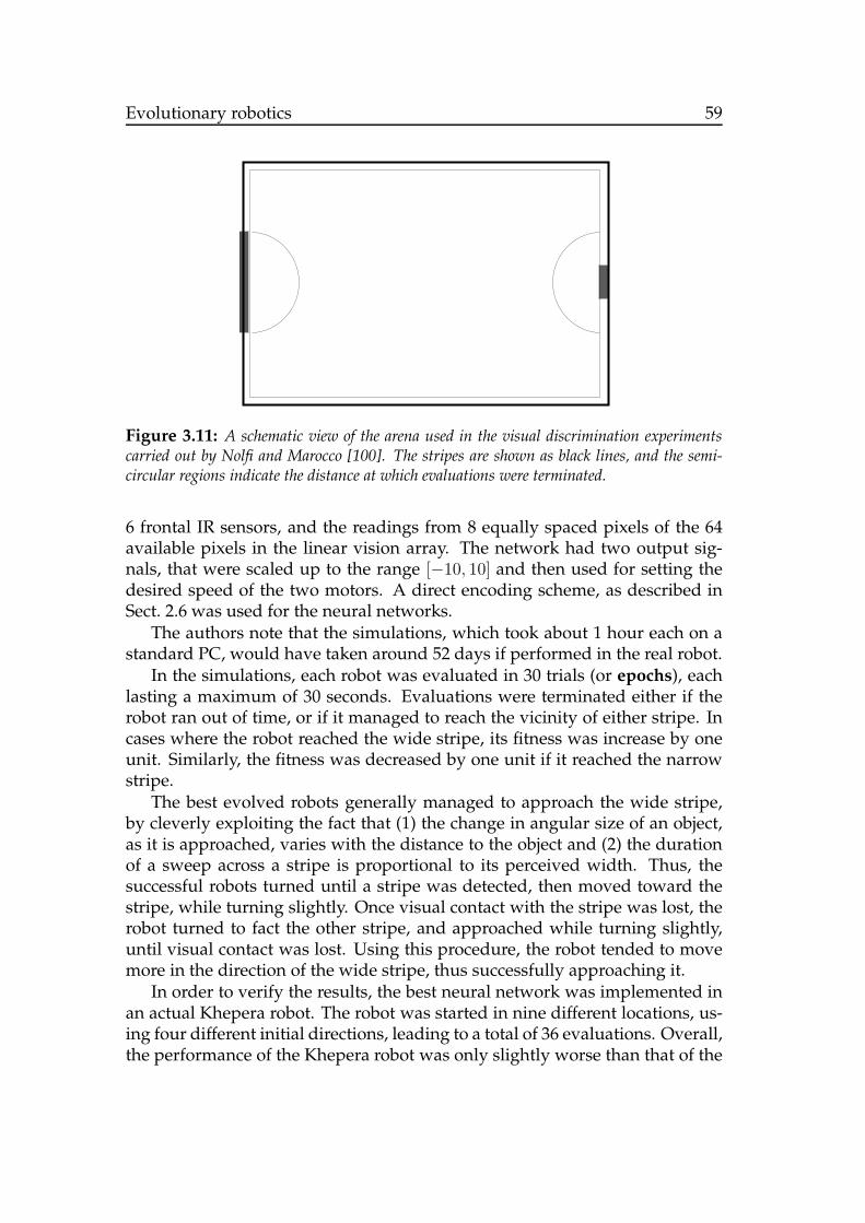
Evolutionary robotics 59
Figure 3.11: A schematic view of the arena used in the visual discrimination experimentscarried out by Nolfi and Marocco [100]. The stripes are shown as black lines, and the semi-circular regions indicate the distance at which evaluations were terminated.
6 frontal IR sensors, and the readings from 8 equally spaced pixels of the 64available pixels in the linear vision array. The network had two output sig-nals, that were scaled up to the range [−10, 10] and then used for setting thedesired speed of the two motors. A direct encoding scheme, as described inSect. 2.6 was used for the neural networks.
The authors note that the simulations, which took about 1 hour each on astandard PC, would have taken around 52 days if performed in the real robot.
In the simulations, each robot was evaluated in 30 trials (or epochs), eachlasting a maximum of 30 seconds. Evaluations were terminated either if therobot ran out of time, or if it managed to reach the vicinity of either stripe. Incases where the robot reached the wide stripe, its fitness was increase by oneunit. Similarly, the fitness was decreased by one unit if it reached the narrowstripe.
The best evolved robots generally managed to approach the wide stripe,by cleverly exploiting the fact that (1) the change in angular size of an object,as it is approached, varies with the distance to the object and (2) the durationof a sweep across a stripe is proportional to its perceived width. Thus, thesuccessful robots turned until a stripe was detected, then moved toward thestripe, while turning slightly. Once visual contact with the stripe was lost, therobot turned to fact the other stripe, and approached while turning slightly,until visual contact was lost. Using this procedure, the robot tended to movemore in the direction of the wide stripe, thus successfully approaching it.
In order to verify the results, the best neural network was implemented inan actual Khepera robot. The robot was started in nine different locations, us-ing four different initial directions, leading to a total of 36 evaluations. Overall,the performance of the Khepera robot was only slightly worse than that of the
Evolutionary robotics 60
simulated robots.
Additional experiments were also performed, using instead an environ-ment containing a small and a large black cylinders, whose sizes varied be-tween different evaluations of the same individual. For more details concern-ing the behavior of the evolved robots in these experiments, see [100].
3.2.4 Corridor-following behavior
Corridor-following could be considered as an instance of the more general be-havior navigation considered above. However, following corridors is an im-portant special case, particularly in indoor applications. Thus, this topic willbe given a brief separate consideration.
In [114], corridor-following behavior was evolved in simulations, using GP.Reynolds’ main point was that previous investigations of corridor-followinghad been fully deterministic and noise-free, leading to brittle results, becauseof the ability of the EA to exploit the particular details of the environmentin question. Reynolds, by contrast, introduced both sensory noise and motornoise in the simulations.
The simulations were performed using a very simple robot model, witha lower limit on its turning radius, essentially forcing it to move along thecorridor in which is was placed. As is common in GP, the structure of therobotic brain was allowed to vary during evolution. The simulated robotswere equipped with simple sensors, measuring wall proximity.
The author chose a fitness measure that encouraged even very slight im-provements. Thus, each individual was evaluated for a maximum of 16 trials.In each trial a graded fitness measure was used, based on the percentage of thecorridor negotiated (without collisions) by the simulated robot, starting from arandom direction of heading, as illustrated in Fig. 3.12. If a robot collided witha wall, it was not allowed to perform further evaluations. Thus, there was aselection pressure in favor of individuals capable of general navigation in thecorridor.
Simulations were performed using either a fixed set of (nine) proximitysensors, or a variable sensor setup, determined by the EA. Thus, in the lat-ter case, both the brain and (part of) the body of the simulated robots wereevolved. As expected, it was found that sensors placed in forward-pointingdirections, were more useful in corridor following than sensors pointing to theside or backwards. A certain degree of lateral symmetry was also found, eventhough the symmetry was not exact. The issue of simultaneous evolution ofbody and brain will be considered in more detail below (see Subsect. 3.4.3).

Evolutionary robotics 61
Figure 3.12: Gradually improved results obtained during the evolution of corridor-following behavior. Reproduced with kind permission of Dr. C. Reynolds.
3.2.5 Behaviors for robot soccer
In recent years, there has been a great interest in robot soccer, manifested inevents such as the Robocup tournament (see www.robocup.org). Robot soc-cer, or indeed any two-person (or two-team) game for robots, leads to interest-ing questions concerning not only evolution of behaviors in general, but alsomulti-robot coordination, co-evolution etc. Research on this topic has resultedin a very large number of publications, and only a few brief examples will begiven here. The interested reader is referred to www.robocup.org for furtherinformation.
The ultimate aim of Robocup is to generate a team of (humanoid) roboticfootball players, capable of beating the best human team, a seemingly distantgoal. In addition to humanoid robot soccer, wheeled robots and simulatedrobots have been used as well in the framework of Robocup. In [70], Lazarusand Hu evolved goalkeeper behavior in simulations using GP. In the simu-lations, the function set (see Sect. 2.6) included the standard operators of ad-dition (add ), multiplication (mult ) etc., as well as problem-specific operatorssuch as e.g. kick and catch . The terminal set included e.g. the directionto the ball and the distance to the ball. Each individual goalkeeper robot wastested against attacks from 10 different directions, as shown schematically inFig. 3.13. An attack consisted of the attacker kicking the ball in a straight linetoward the goal. The authors attempted to evolve active goalkeepers, thatwould not only catch an incoming ball, but would also attempt actively to
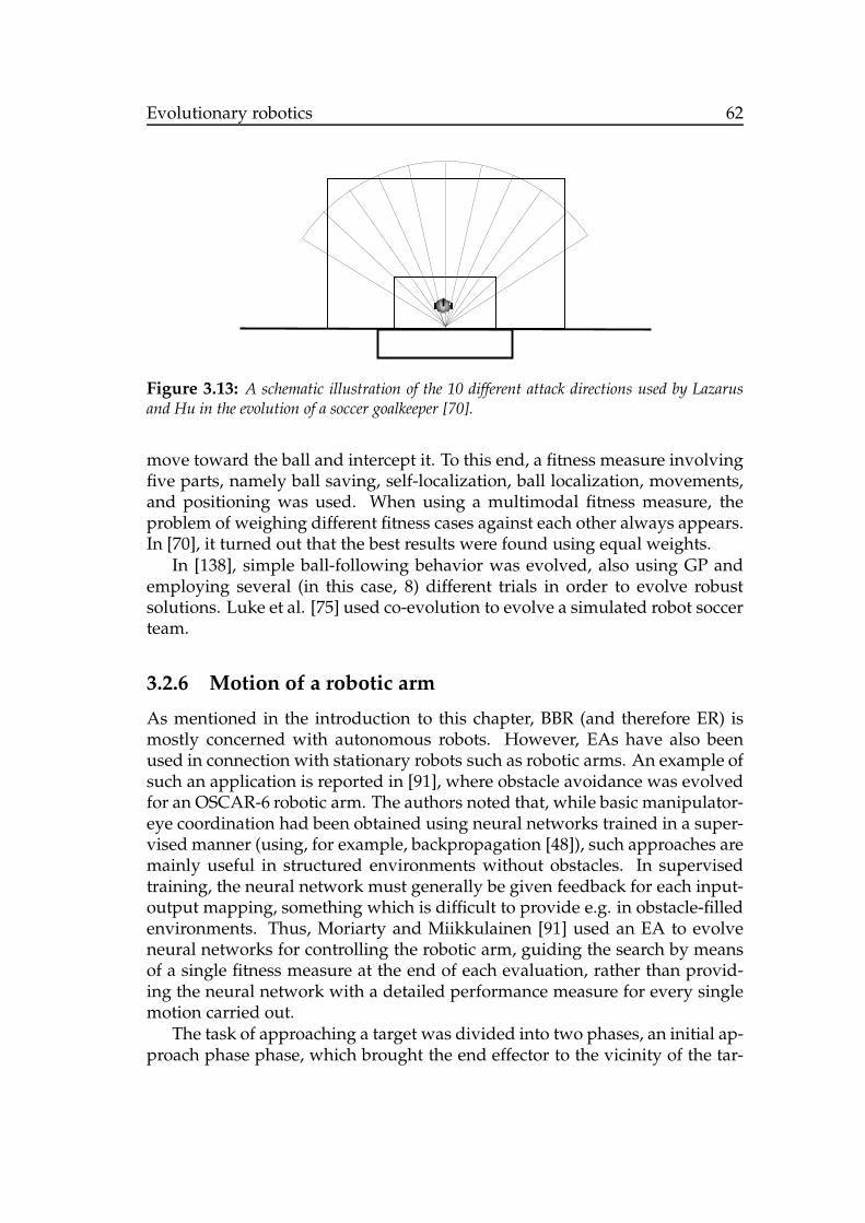
Evolutionary robotics 62
Figure 3.13: A schematic illustration of the 10 different attack directions used by Lazarusand Hu in the evolution of a soccer goalkeeper [70].
move toward the ball and intercept it. To this end, a fitness measure involvingfive parts, namely ball saving, self-localization, ball localization, movements,and positioning was used. When using a multimodal fitness measure, theproblem of weighing different fitness cases against each other always appears.In [70], it turned out that the best results were found using equal weights.
In [138], simple ball-following behavior was evolved, also using GP andemploying several (in this case, 8) different trials in order to evolve robustsolutions. Luke et al. [75] used co-evolution to evolve a simulated robot soccerteam.
3.2.6 Motion of a robotic arm
As mentioned in the introduction to this chapter, BBR (and therefore ER) ismostly concerned with autonomous robots. However, EAs have also beenused in connection with stationary robots such as robotic arms. An example ofsuch an application is reported in [91], where obstacle avoidance was evolvedfor an OSCAR-6 robotic arm. The authors noted that, while basic manipulator-eye coordination had been obtained using neural networks trained in a super-vised manner (using, for example, backpropagation [48]), such approaches aremainly useful in structured environments without obstacles. In supervisedtraining, the neural network must generally be given feedback for each input-output mapping, something which is difficult to provide e.g. in obstacle-filledenvironments. Thus, Moriarty and Miikkulainen [91] used an EA to evolveneural networks for controlling the robotic arm, guiding the search by meansof a single fitness measure at the end of each evaluation, rather than provid-ing the neural network with a detailed performance measure for every singlemotion carried out.
The task of approaching a target was divided into two phases, an initial ap-proach phase phase, which brought the end effector to the vicinity of the tar-

Evolutionary robotics 63
get, and a final approach phase which used smaller movements to reach withingrasping distance of the target. Based on this division, the authors devised acontrol system consisting of two neural networks, a primary network for theinitial approach phase, and a secondary network for the final approach phase.Each network was represented as a fully connected FFNN, with 9 input units,a single hidden layer with 16 neurons, and 7 output neurons. The 9 input unitsconsisted of 6 proximity sensors, as well as the x, y, and z components of thedistance between the end effector and the target. Six of the output units wereused for determining the direction of rotation and magnitude of rotation forthree joints in the robotic arm. The output units determining the magnitudeof rotation were scaled differently in the primary and secondary networks, insuch a way that the motion of the secondary networks used smaller steps. Theseventh output unit was used to override the output of the other six outputs,and thus to stop the arm, in emergency situations.
The training of the arms was made by starting the arm with random jointpositions, and a random target position, selected from a set of 400 pre-generatedpositions. An additional 50 target positions were generated for use during test-ing. In addition, obstacles were placed in one of 12 imaginary boxes locatedin the path of robotic arm. The motion was executed as a series of discretemoves, and simulations were terminated e.g. if a collision occurred. Fitnesswas assigned as the percentage of the initial distance (between the position ofthe end effector and the target) covered during the motion.
The results of the EA showed that the combination of primary and sec-ondary networks could, in fact, control the arm to within industry standards,i.e. with a deviation of one cm or less between the actual and desired end ef-fector positions. Furthermore, using the 50 test cases, it was shown that theevolved solutions were robust; Obstacles were hit only in around 2% of thetest cases.
3.3 Evolution of complex behaviors and behavioral
organization
A central issue in BBR is behavioral organization (also known as behavioralcoordination, behavior arbitration, or action selection), i.e. the process of de-termining which behavior to activate at a given time. Several methods for be-havioral organization have been suggested, e.g. subsumption [14], activationnetworks [78], potential fields [64], distributed architecture for mobile naviga-tion (DAMN) [115]. For reviews of such methods see e.g. [3], [9], and [108].
However, in many methods suggested to date, it is not uncommon, aspointed out in [9], [79], and [131], that the user must specify the architectureof the behavioral organization system by hand. This is far from optimal, for

Evolutionary robotics 64
several reasons: First, as mentioned in Subsect. 3.1.1, behavior-based robotsare generally expected to operate in unstructured environments, which cannoteasily be predicted, making it difficult to tune parameters by hand. Second,even if the environment happens to be fairly well structured, it is difficult to as-sess (at least quantitatively) the relevance of some behaviors, especially thosethat are not directly related to the assigned task of the robot. For example, abattery-driven robot that is assigned the task of transporting goods betweentwo locations, must occasionally recharge its batteries. Clearly, the behaviorof charging batteries is important, but it is difficult to judge quantitatively itsrelevance against the relevance of the assigned task, and thus to assign an opti-mal reward for it. Third, hand-coding a behavioral organizer represents a stepaway from the biologically inspired behavior-based architecture.
The purpose of any method for behavioral organization is to determinewhen different behaviors should be activated, and it is therefore natural tocategorize methods of behavioral organizations based on the procedure theyuse for selecting behaviors. There are two main categories, namely arbitrationmethods and cooperative methods3. In arbitration methods, exactly one be-havior is active, and the selection of which behavior to activate is generally afunction both of present sensor readings and the internal state of the robot. Incooperative methods, the action taken by the robot is a weighted combinationof the actions suggested by several behaviors.
The problem of behavioral selection has, of course, also been heavily stud-ied in the field of ethology (see e.g. [30] for a review). The brains of biologicalorganisms have been optimized through millions of years of evolution result-ing in behavioral selection systems, manifested in the beliefs and desires ofthe organism, that maximize the chances of survival. Thus, the concepts andideas introduced in ethology should be carefully considered when proposingmethods for behavioral selection in robotics.
From the point of view of ER, the aim, of course, is to reach beyond the sim-ple (and often purely reactive) robotic brains described above, and thus to gen-erate robotic brains capable of more complex behaviors. However, not all suchstudies have centered on behavioral organization in the sense described above,let alone evolution of behavioral organization. Basically, the published studiesthat focus on the evolution of complex behaviors can be divided into threecategories, namely (1) those in which complex behaviors are evolved withoutexplicit behavioral selection, i.e. without the presence of an independentlygenerated behavioral organizer that selects which behavior to activate [34],[44], [67], [94], [137], (2) those in which behaviors are evolved independentlyand are then used in a complete robotic brain equipped with a behavioral or-ganizer which is not evolved itself [65], and (3) those in which the central issueis the evolution of the behavioral organizer, and where the individual behav-
3Cooperative methods are sometimes also called command fusion methods.

Evolutionary robotics 65
2000 4000 6000 8000
60
70
80
90
100
f
i
Figure 3.14: Maximum fitness as a function of the number of evaluated individuals duringthe evolution of a complex behavior, divided into two constituent behaviors [137]. The threeshort and almost vertical curves show the results from runs in which the constituent behaviorswere first evolved separately, and then combined to form the complete robotic brain.
iors are generated either through an EA or by other means [71], [131].Here, ashort description of each category will be given, with the strongest emphasisplaced on the third category (see Subsect. 3.3.3 below), for which the utilityfunction method [131] will be described in some detail.
3.3.1 Complex behaviors without explicit arbitration
As pointed out in [44] and [137], a common problem when evolving com-plex behaviors is that the difference between the initial, randomly generated,robotic brains and those capable of carrying out the desired complex behavior,is so large that the EA without exception finds itself stuck in a local optimum.One obvious solution is to break down the problem into simpler tasks, forwhich the EA will be able to find an adequate solution, and then either to fuseseveral evolved robotic brains into one complete brain [137], or to make theproblem progressively more difficult until the desired level of complexity isreached, a procedure called incremental evolution [44].
An example, taken from [137], is shown in Fig. 3.14. Here, the task was toevolve a complex robotic brain, capable both of cleaning an arena and avoidingmoving obstacles. Two different approaches were used, namely (1) attemptingto evolve the complex behavior directly, starting from random robotic brains(which, in this investigation, were represented by generalized FSMs, see Ap-pendix C), and (2) first evolving cleaning and evasion separately, then fusingthe two generalized FSMs by adding random connections between them and,finally, continuing the evolution until the complex behavior emerged. In Fig.
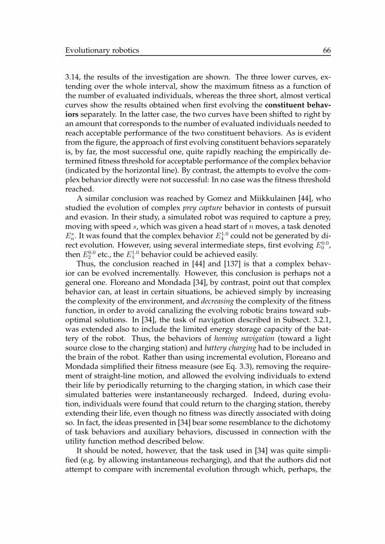
Evolutionary robotics 66
3.14, the results of the investigation are shown. The three lower curves, ex-tending over the whole interval, show the maximum fitness as a function ofthe number of evaluated individuals, whereas the three short, almost verticalcurves show the results obtained when first evolving the constituent behav-iors separately. In the latter case, the two curves have been shifted to right byan amount that corresponds to the number of evaluated individuals needed toreach acceptable performance of the two constituent behaviors. As is evidentfrom the figure, the approach of first evolving constituent behaviors separatelyis, by far, the most successful one, quite rapidly reaching the empirically de-termined fitness threshold for acceptable performance of the complex behavior(indicated by the horizontal line). By contrast, the attempts to evolve the com-plex behavior directly were not successful: In no case was the fitness thresholdreached.
A similar conclusion was reached by Gomez and Miikkulainen [44], whostudied the evolution of complex prey capture behavior in contests of pursuitand evasion. In their study, a simulated robot was required to capture a prey,moving with speed s, which was given a head start of nmoves, a task denotedEs
n. It was found that the complex behavior E1.04 could not be generated by di-
rect evolution. However, using several intermediate steps, first evolving E0.00 ,
then E0.02 etc., the E1.0
4 behavior could be achieved easily.Thus, the conclusion reached in [44] and [137] is that a complex behav-
ior can be evolved incrementally. However, this conclusion is perhaps not ageneral one. Floreano and Mondada [34], by contrast, point out that complexbehavior can, at least in certain situations, be achieved simply by increasingthe complexity of the environment, and decreasing the complexity of the fitnessfunction, in order to avoid canalizing the evolving robotic brains toward sub-optimal solutions. In [34], the task of navigation described in Subsect. 3.2.1,was extended also to include the limited energy storage capacity of the bat-tery of the robot. Thus, the behaviors of homing navigation (toward a lightsource close to the charging station) and battery charging had to be included inthe brain of the robot. Rather than using incremental evolution, Floreano andMondada simplified their fitness measure (see Eq. 3.3), removing the require-ment of straight-line motion, and allowed the evolving individuals to extendtheir life by periodically returning to the charging station, in which case theirsimulated batteries were instantaneously recharged. Indeed, during evolu-tion, individuals were found that could return to the charging station, therebyextending their life, even though no fitness was directly associated with doingso. In fact, the ideas presented in [34] bear some resemblance to the dichotomyof task behaviors and auxiliary behaviors, discussed in connection with theutility function method described below.
It should be noted, however, that the task used in [34] was quite simpli-fied (e.g. by allowing instantaneous recharging), and that the authors did notattempt to compare with incremental evolution through which, perhaps, the

Evolutionary robotics 67
sensors nodes goals
In battery charging area
Near battery charging area
Light level is low
Nothing around the robot
Obstacles are close
Following light Charging battery
Moving in straight line
Avoiding obstacles
Full battery
Not zero battery
Figure 3.15: A schematic representation of the behavioral organizer used by Kim and Cho[65]. The dashed lines are successor links and the solid ones are predecessor links, asdefined in the method of activation networks [79].
complex behavior could have evolved even faster. Nevertheless, the resultsreported above show that there are several ways of achieving complex behav-iors.
In addition, Floreano and Mondada carried out a painstaking analysis oftheir evolved neural network, in order to determine how it generated the com-plex behavior. While their analysis was impressive, it does, perhaps, point to aweakness with respect to the use of neural networks. The advantages of neu-ral networks, i.e. noise tolerance, absence of bias introduced by the user etc.,have been eloquently presented by several authors (e.g. [19], [34], and [94]).However, neural networks are also notoriously difficult to interpret. Thus, acomplex behavior based on neural networks will, most often, have to be usedas a black box. An alternative approach is to consider the robotic brain as atwo-part system containing (1) a set of basic behaviors, which may be imple-mented as neural networks, but also in other ways, using e.g. finite-state ma-chines or if-then-else -rules, and (2) a behavioral organizer (or arbitrator)that dynamically selects which behavior to activate, at all times. Such systemswill be introduced in the two following subsections.
3.3.2 Evolving behavioral repertoires
Kim and Cho [65] evolved a set of behaviors (also called a behavioral reper-toire [131]) for a task similar to the homing navigation considered by Floreanoand Mondada [34]. Their repertoire consisted of four behaviors, namely charg-

Evolutionary robotics 68
ing battery, following light, avoiding obstacles, and moving in a straight line. Foreach behavior, a neural network known as a CAM-brain (based on cellularautomata) was evolved, using incremental evolution [44]. However, the be-havioral organizer was not evolved. Instead the method of activation networks[78], [79] was used. Kim and Cho found that the behavioral organization sys-tem was able to select behaviors in the appropriate order, so as to achieve themain task of navigating in the arena, without collisions and without runningout of battery energy.
As pointed out above, an advantage of their behavioral organizer, com-pared to complex behaviors implemented in a neural network, is its relativesimplicity, as indicated in Fig. 3.15. However, the method of activation net-works, as indeed most methods of behavioral organization, requires that theuser be able to set a large number of properties manually, something whichbecomes more and more difficult as the size and complexity of the behavioralrepertoire grows.
Thus, as an alternative to such methods, one may evolve the behavioral or-ganizer itself. To conclude this section, one such method will now be describedin some detail.
3.3.3 Evolution of behavioral organization by means of the
utility function method
The utility function method developed by Wahde [131] is a biologically in-spired arbitration method, in which the selection of behaviors is based on aquantity called utility. Thus, before the method itself is described, a shortintroduction will be given to the concept of utility and its uses in rationaldecision-making.
Utility and rational decision-making
The concept of utility is used both for studying decision-making in economictheory and for studying behavioral selection in ethology. 4
Consider a case in which a robot must decide which of n actions A1, A2, . . . ,An to perform. For simplicity, consider the case n = 3, and assume that theactions have been ordered according to preference, such that the robot prefersA1 to A2, and A2 to A3. The situation can be denoted A1 > A2, A2 > A3, where> in this case means “is preferred to”. If this is the case, then A1 must also bepreferred to A3, so that A1 > A2 > A3. This property, known as transitivity ofchoice, underlies all rational decision-making. An agent exhibiting transitivity
4In ethology, the terms benefit or negative cost are often used instead of utility. Here,however, the term utility with be used throughout.

Evolutionary robotics 69
of choice is called a rational agent. Note that the use of reason is not a neces-sary prerequisite for rationality. Rational choices can be made unwittingly as aresult of design, as is the case in reactive robots and most likely in insects and,probably, in many higher animals as well.
In order to rank possible actions in order of preference, a common currencymust be available. Furthermore, it can be shown (see e.g. [30], [31], and [32])that an agent with transitive preferences uses a maximimization procedure,i.e. will select the action whose value, measured in the common currency, ismaximal. The common currency is usually called utility, and a rational agentthus selects the action to perform (Aisel) according to
Aisel = argmax U(Ai), (3.14)
where U(Ai) denotes the utility of action Ai in the current situation.
As an example, consider a floor-sweeping robot, which is given a fitnessincrement for each square meter of floor it sweeps. Clearly, the robot should tryto sweep as much floor as possible, in order to maximize its fitness. However,if the robot runs out of battery energy, it will no longer be able to move. Thus,the utility of a behavior that forces the robot to suspend, temporarily, its floor-sweeping activities to charge its batteries will rise as the energy in the batterydecreases, even though the battery charging behavior does not lead to anydirect increase in fitness. Hence, in order to receive as much fitness as possibleover a long period of time, the robot must, in fact, maximize utility.
Utility also provides a means of allocating limited resources in an optimalway. The life of any animal (or robot) inevitably involves many trade-offs,where less relevant behaviors must be sacrificed or at least postponed in orderto perform the most relevant behaviors, i.e. those associated with largest utilityvalue.
Organizing behaviors using the utility function method
In the utility function method [131], the robot is equipped with a behavioralrepertoire, in which each behavior Bi is assigned a utility function Ui, whichdepends on the values of the state variables of the robot. Three kinds of statevariables are defined, namely external variables, denoted s, representing e.g.sensor readings, internal physical variables, denoted p, representing e.g. theenergy in the batteries of the robot, and internal abstract variables, denoted x,which are dimensionless variables used in the behavioral selection procedure,and which roughly correspond to signalling substances (e.g. hormones) inbiological systems. Thus, the most general form of a utility function is
Ui = Ui
(
s1, . . . , sne, p1, . . . , pnp, x1, . . . , xni
)
, (3.15)

Evolutionary robotics 70
46 48 50 52 54 56time
-10
-5
0
5
10
utili
ty
B3
B2
B1
Figure 3.16: The utility functions for a behavioral organization problem, shown as functionsof time during part of the evaluation of a simulated robot.
where ne, np, and ni denote the number of external, internal physical, andinternal abstract variables, respectively. However, in most cases, each utilityfunction will only depend on a subset of the set of available variables.
In the utility function method, behaviors are divided into two categories.Task behaviors are directly related to the task of the robot and increase itsfitness, if successfully executed. An example of a task behavior is the floor-sweeping behavior described in the example above. Auxiliary behaviors, onthe other hand, do not change the fitness of the robot, but are neverthelessnecessary for the robot to be able to perform its duties. The battery chargingbehavior (for the floor-sweeping robot described above) is an example of anauxiliary behavior.
Furthermore, a time variable ti, referred to as the behavior time of behav-ior Bi, is defined for all behaviors. ti is set to zero every time Bi is activated,and then follows the same rate of increase as the global time variable t, whichmeasures the time since the robot was initialized. As soon as behavior Bi be-comes inactive, ti is again set to zero, where it remains until the behavior isactivated again.
Behavioral selection is straightforward in the utility function method; Atregular intervals, the values of the utility functions are computed, using thelatest available readings of the state variables as input, and the behavior withthe highest utility value is executed. This is illustrated in Fig. 3.16, in which isshown the variation in time of three utility functions obtained for a behavioralorganization problem involving three behaviors. In the part of the simulationshown in the figure, behavior B2 is initially active, since its utility value ex-

Evolutionary robotics 71
ceeds that of the other behaviors, and remains active from t = 44 (arbitraryunits) until around t = 49.5, when B3, which in this case happened to be anauxiliary battery charging behavior, was activated. Around t = 56, B1 wasactivated.
The problem, of course, is to determine the shape of the utility functions.In the utility function (UF) method, the optimization of utility functions is nor-mally carried out using EAs. In general, the utility functions depend on severalstate variables, and should provide appropriate utility values for any combi-nation of the relevant inputs. Thus, determining the exact shape of the utilityfunctions is a formidable task, and one for which EAs are very well suited. Inprinciple, GP can be used, in which case any function of the state variables canbe evolved. However, it is often sufficient to make an ansatz for the functionalform of each utility function, and then implement the EA as a standard GA forthe optimization of the parameters in the utility function.
For example, for a utility function Ui (associated with a behavior Bi) thatdepends on the two variables s and p, a common ansatz is
Ui(s, p) = ai,00 + ai,10s+ ai,01p+ ai,20s2 + ai,11sp+ ai,02p
2, (3.16)
where the ai,jk are constants. When optimizing the utility functions the ai,jk
(and the corresponding constants in all other utility functions), should be en-coded in the chromosomes used by the GA. The fitness gained while executingthe task behavior(s) is used as the optimization criterion.
A problem that may occur when selecting behaviors based on utility func-tions is rapid behavior switching in which the robot keeps swapping back andforth between two (or more) behaviors, and thus failing to achieve its goals.One of the purposes of the internal abstract variables is to prevent such rapidswitching. Thus, an internal abstract variable xi, which takes non-zero valuesonly in a specific behavior Bi, can be introduced. When the robot switchesfrom another behavior to Bi, xi is immediately set to a non-zero value (e.g.1), and if the utility functions are properly chosen, the utility of Bi will thenbe raised sufficiently to avoid immediate switching to another behavior. Asan example consider, in Fig. 3.16, the jump in utility for B3 at the momentwhen it becomes active. The internal abstract variables may depend both onother state variables and on the behavior time ti, and the exact variation canbe optimized by the GA as well. For example, a possible ansatz for an internalabstract variable xi is
xi =
{
bi,1 + bi,2e−|bi,3|ti If Bi is active
0 Otherwise(3.17)
where the bi,j are constants. Thus, with this ansatz for the internal abstractvariables, the chromosomes used by the GA will encode not only the constantsai,jk, but the constants bi,j as well.

Evolutionary robotics 72
Robotic brain
B1 B2 B3
B3.1
B3.2
Figure 3.17: An example of a robotic brain involving five behaviors on two hierarchical levels,taken from [136].
Behavioral hierarchies
The presentation above is somewhat simplified, in that it does not consider thefact that, in order to keep the level of complexity of the constituent behaviorsin a robotic brain at a reasonable level, the behaviors should often be dividedinto sub-behaviors. Battery energy maintenance is a case in point: maintain-ing the energy in the batteries of a robot requires that (at least) two separateprocedures be executed: one for finding an energy source, and one for connect-ing to the energy source and carrying out the actual charging. Evidently, theentire energy maintenance sequence could be considered as one single behav-ior. However, generating such a behavior, and making it reliable, for examplein the case of sudden interruptions due to obstacles in the path of the robot,would indeed be a daunting task. An alternative procedure is to introduce onebehavior for locating an energy source, and one for battery charging, and toconsider these behaviors as sub-behaviors to an overall energy maintenancebehavior. Thus, in such a case, the robotic brain would have a hierarchicalstructure, an example of which is shown in Fig. 3.17.
This figure shows the structure of the robotic brain for a simple, two-wheeledguard robot considered in [136]. The behavioral repertoire consisted of a totalof five behaviors, namely straight-line navigation (B1), obstacle avoidance (B2),energy maintenance (B3), corner seeking (B3.1), and battery charging (B3.2). In thearena where the robot operated, the battery charging stations were placed inthe corners. Thus, the corner seeking behavior corresponded to charging stationlocalization.
As shown in the figure, the five behaviors were placed on two hierarchicallevels. The utility function is able to cope with multiple hierarchical levels ofbehaviors, by comparing utility values on a level-by-level basis. Thus, in the

Evolutionary robotics 73
Robot with
3 sensors
Moving
obstacleArena border
Figure 3.18: The arena used in [107]. The aim of the simulated robot is to move withoutcollisions, from right to left, in the arena.
Figure 3.19: The robot used in [107] as seen from above, equipped with three simple prox-imity sensors, each with a triangular-shaped detection range. The filled black circles illustratepoints on an obstacle that are detectable by the range sensors. Dashed lines indicate detectedpoints in this particular configuration.
case shown in Fig. 3.17, it was determined which of the three utility functionsU1, U2, and U3 took the highest value. If it happened to be U3, the comparisonof U3.1 and U3.2 would determine which of these two behaviors was active.
The procedure is actually slightly more complex than this since the switchfrom, say, B2 to B3 (and then to one of the sub-behaviors B3.1 or B3.2) may re-quire modification of the internal abstract variables (if any) in B3, in order toavoid rapid behavior switching as discussed above. In practice, this is accom-plished by executing an enter procedure on each hierarchical level. Thus, whenU3 exceeded U2, the enter procedure for U3 was executed (thus possibly furtherraising U3 to prevent rapid switching back to B2), Next, the enter procedure ofeither B3.1 or B3.2 was called, depending on their relative utility values, andthe robot then proceeded by executing the active behavior, i.e. either B3.1 orB3.2.

Evolutionary robotics 74
0 1 2 3 4 5 6 7Time (s)
0
1
2
3
Util
ity
Figure 3.20: The early stages of a typical run. The bottom right panel shows the varia-tion of the four utility functions in one of the best performing individuals during evolutionwith the dynamic model. The curves represent the utility values for the behaviors move for-ward (solid curve), move backward (dash-dotted curve,), stop (dotted curved), and charge(dashed curve). Note that the utility of the move backward behavior is very low throughoutthe simulation.
Example 1: Locomotion in an arena with moving obstacles
In [107], the utility function method was used for generating a behavioral or-ganization system for a hopping robot traversing an arena with moving ob-stacles, illustrated in Fig. 3.18. The simulated robot, consisting of a foot plateand a leg with two degrees of freedom (DOF), implemented as two revolutejoints, was equipped with four behaviors: move forward (B1), move backward(B2), stop (B3), and charge batteries (B4). The robot was simulated using fullnewtonian dynamics, implemented in the EvoDyn package developed by Pet-tersson [104]. In B4, the robot was required to remain at a standstill, chargingits batteries using simulated solar cells.
While the UF method itself uses an EA to generate behavioral organization,the constituent behaviors can be generated by any method. In the particularcase considered in [107], the behaviors were implemented as continuous-time,recurrent neural networks (see Appendix A), and were optimized using an EA.Note, however, that the EA optimizing the individual behaviors should not beconfused with the EA used for generating the behavioral organizer throughthe UF method.
Once the four constituent behaviors had been generated, the behavioral

Evolutionary robotics 75
97 97.5 98 98.5 99 99.5 100Time (s)
-0.6
-0.5
-0.4
-0.3
-0.2
-0.1
0
Util
ity
Figure 3.21: A behavior switching sequence where, at first, behavior B1 (move forward) isactive. Shortly thereafter behavior B4 (charge) is activated due to the detection of an approach-ing obstacle. As the obstacle passes, and the sensor signal decreases, B1 is activated again. Forclarity, only the utility values for B1 (solid line) and B4 (dashed line) are shown in the bottompanel.
organizer, assigned the task of selecting between behaviors B1-B4, was gen-erated using the utility function method. The simulated robot was equippedwith three proximity sensors, as illustrated in Fig. 3.19. In addition, the robotwas able to measure the amount of available energy in its batteries. Thus,the ansatz for each utility function was taken as a second-degree polynomialUi = Ui(s1, s2, s3, E, xi), where s1, s2, and s3 are the readings of the three sen-sors, E is the battery energy, and xi is a behavior-specific internal abstractvariable, whose variation was modelled as in Eq. (3.17). The total numberof parameters to be optimized by the GA was 96.
The settings of the simulated robot’s battery were such that frequent recharg-ing was necessary. Thus, the task of moving through the arena was stronglynon-trivial, requiring constant vigilance in order to avoid collisions or an emptybattery (in which cases the evaluation was terminated). The fitness measurewas simply taken as the distance moved in the forward direction.
Despite the many parameters determining the utility functions and the ab-stract internal variables, a successful behavioral organizer was found quitequickly. An example is shown in Fig. 3.20, and a movie of the robot is availableon the tutorial CD in the file HoppingRobot_BehavioralOrganization.mpg .
However, the dynamically simulated robot was unable to traverse the wholearena. The failure could be attributed to the limited quality of the constituent

Evolutionary robotics 76
Figure 3.22: A two-wheeled exploration robot in a simple arena with 5 stationary obstacles.
behaviors B1-B4, rather than a failure of the behavioral organization system.Thus, an obvious conclusion was that the constituent behaviors must at leastreach some minimum level of quality, in order for a behavioral organizer toperform well.
In order to study the evolution of behavioral organizer in its own right, Pet-tersson and Wahde also carried out some simulations using a much simplerdynamical model (essentially a point-particle model) for the simulated robots.In this case, the EA found utility functions that would allow the robot to tra-verse the entire arena without collisions. An example of the motion of the sim-plified robot is shown in Fig. 3.21. In addition, two movies are available on thetutorial CD, in the files SimpleRobot_UM1.mpg and SimpleRobot_UM2.mpg .
Example 2: A simple exploration robot
As a second example of an application of the utility function method, a sim-ple exploration robot will be considered. The two-wheeled robot, shown inFig. 3.22, is differentially steered, and equipped with a two-dimensional laserrange finder for measuring the distance to the nearest objects in a certain sec-tor. In this example, the sector of measurement will be assumed to cover anarrow range centered around the current direction of motion of the robot.The task of this robot will be to explore a given arena, also shown in Fig. 3.22,while avoiding collisions with stationary obstacles.
Obviously, in a more realistic application, the robot would have to be able
Evolutionary robotics 77
to find a charging station and charge its batteries when necessary, avoid mov-ing obstacles (in addition to stationary ones), and carry out purposeful motionrather than the more or less random wandering that will be considered here.In such cases, a rather complex robotic brain involving many behaviors, prob-ably distributed on various hierarchical levels, e.g. as illustrated in Fig. 3.17,would be needed. The utility function method would easily handle such asituation, but, for simplicity and clarity, a greatly simplified situation will bestudied in this example, where the capacity of the robot’s battery is assumedto be infinite. In fact, only two behaviors will be included in the robotic brain,namely straight-line navigation (B1) and obstacle avoidance (B2). In B1, the brainof the robot sends equal signals to the two motors of the robot, making it movein a straight line (after an initial transient, in case the robot was turning at thetime of activation of B1). In B2, equal signals, but of opposite sign, will be sentto the two motors, until the minimum distance (as measured by the laser rangefinder) to the nearest obstacle exceeds a certain minimum value.
The fitness measure is basically taken as the amount of time spent execut-ing B1. However, the robot receives a fitness increase only if it executes B1
continuously for at least T0 seconds. The value of T0 was chosen, somewhatarbitrarily, as 0.2 s. With this fitness measure, the robot has a strong incentivefor executing B1 as much as possible, without dithering between the two be-haviors. On the other hand, it is also necessary for it sometimes to activateB2, in order to avoid collisions, since the evaluation is terminated if the robotcollides with a wall or with some other obstacle. Thus, the robot is faced witha behavioral selection problem, involving a trade-off between carrying out theassigned task (by executing B1) and surviving (by executing B2). Clearly, inthis simple case, it would not have been very difficult to write down a pro-cedure for behavioral selection by hand. However, as indicated above, thissimple example of a behavioral selection problem was chosen primarily for its(intended) pedagogical value, not for its (rather limited) usefulness.
In order to apply the utility function method, an ansatz is needed for eachutility function. Here, U1 will be taken as a pth degree polynomial in the vari-ables s1, s2, and s3 which represent the (inverted) readings along three rays ofthe laser range finder (in the directions 0, ± 30 degrees, relative to the forwarddirection). The inverted reading y along a ray equals R − z, where R is themaximum range (4.0 m, in this case) of the laser range finder, and z is the mea-sured distance to the nearest object along the ray. Thus, y will be in the range[0, R]. For B2, the utility function (U2) depends on two variables: savg, whichequals the average reading of all rays of the laser range finder and x, which isan internal abstract variable. x can be interpreted as a hormone whose levelis raised if the robot senses fear, e.g. as a result of an imminent collision. Thevariation of the variable x is slightly simplified in this example, however: ittakes the value 0 if B1 is active, and the value 1 if B2 is active.
Thus, the utility functions U1 and U2 will be polynomials of three and two
Evolutionary robotics 78
2 4 6 8 10Time
-3
-2
-1
0
1
2
3
4
Util
ity
Figure 3.23: Left panel: The motion of the robot, whose initial position is marked by a blackdisk. Right panel: The variation of the utility functions for the first 10 seconds of the motion.The solid line shows U1, and the dashed line U2.
variables, respectively, i.e.
U1(s1, s2, s3) = a000 + a100s1 + a010s2 + a001s3 + a110s1s2 + . . . , (3.18)
and
U2(savg, x) = a00 + a10savg + a01x+ a20s2avg + a11savgx+ a02x
2 + . . . (3.19)
Thus, the task of the evolutionary algorithm will be to determine the coeffi-cents aijk and aij so as to maximize the fitness of the robot in evaluations of agiven maximum duration T (here set to 50 s).
The two behaviors B1 and B2 were implemented in the format defined bythe UF Library simulation package described in Sect. 3.4.4. Next, an exe-cutable application was built, and the simulations for this exploration robotwere carried out, using utility function polynomials of degree p = 2. Due tothe simplicity of the problem, the evolutionary algorithm rather quickly foundrobotic brains that were able to keep the robot from colliding with obstacles forthe full duration of an evaluation, while spending as much time as possible ex-ecuting B1. In the left panel of Fig. 3.23, the motion of an evolved individualis shown, seen from above. The right panel of the same figure shows the vari-ation of the utility functions for the first 10 seconds of the evaluation. At theinitial moment of the evaluation, the robot was placed right in front of an ob-stacle, forcing it first to activate B2 in order to rotate to a different direction(this part of the motion is not visible in the left panel of Fig. 3.23, which onlydisplays translational motion). Once a clear path was found, at t ≈ 2 seconds,the robot began executing B1. At t ≈ 5.5 seconds, another obstacle was en-

Evolutionary robotics 79
countered, and the robot again activated B2 for a fraction of a second, beforeresuming the execution of B1.
3.3.4 Closing comments on behavioral organization
In the description of methods for behavioral organization above, the consid-ered applications were focused on motor behaviors, i.e. behaviors involvingthe actuators (e.g. the wheels) of the robot. Indeed, most methods for behav-ioral organization have, in practice, been applied to navigation-related prob-lems. Thus, while behavioral organization make possible the developmentof slightly more complex robotic brains than can easily be implemented us-ing single behaviors, there is still a long way to go in order to reach the goalof truly intelligent behavior-based robots. An obvious step in that directionwould be to allow purely mental processes, i.e. processes that do not involvethe use of the robot’s actuators, to run in parallel with the motion-related be-haviors (which can then be organized either through cooperative methods orarbitration methods). Indeed, this is the goal of the development of the succes-sor to the utiliy function method, currently in progress in the author’s researchgroup.
3.4 Other issues in evolutionary robotics
ER is a vast field, and this tutorial does not, of course, completely cover allaspects of the field. In the rest of this section, four different topics will beconsidered briefly, namely (1) ER applied to balancing, walking, and hoppingrobots, which constitute an increasingly important special case, (2) the relationbetween simulations and evolution in hardware (i.e. on actual robots) in ER,(3) simultaneous evolution of body and brain of robots, and (4) simulationsoftware for ER.
In addition to these topics, there are many others which will not be cov-ered in detail, such as (1) the relation between evolution and learning in ER,i.e. modification of the brain of a robot during its operation [8], [35], [96], [122],[128], [129], [145], (2) interactive evolution, in which the user provides a sub-jective fitness measure [60], [77], (3) evolvable hardware [63], [81], [126], (4)swarm robotics (see e.g. www.swarm-robotics.org ) and the evolution ofmulti-robot (collective) behaviors [7], [93], [111], [112], [127], (5) co-evolution,i.e. simultaneous evolution of two (or more) populations in competition witheach other, see Subsect. 2.7.3 above and e.g. [21], [36], [75], [101], [132], and (6)behavior acquisition, i.e. the generation of behaviors from primitive actions[143].
Evolutionary robotics 80
3.4.1 Balancing, walking, and hopping robots
In this subsection, the use of evolutionary techniques in connection with theimportant special case of robots equipped with legs rather than wheels will beconsidered, starting with a brief, general survey of walking robots.
Walking robots
Attempts at building walking robots can be traced back at least to the 1960s.In addition to research concerning bipedal robots efforts were also made todevelop monopedal [113] and quadrupedal robots [41]. One of the first func-tioning bipedal robots was developed in the 1970s by Kato [61].
As the name implies, the term bipedal robot refers to a robot that walks ontwo legs, whereas the definition of the term humanoid robot is more loose. Ingeneral, a humanoid robot is defined as a robot with some human-like features(not necessarily the ability to walk on two legs). For example, some humanoidrobots consist only of an upper body or a head (see e.g. [89]).
Some impressive examples of humanoid robots include the Honda ASIMOrobots (world.honda.com/ASIMO) and the Sony QRIO robots (www.sony.net/SonyInfo/QRIO). Advanced quadrupedal robots have also been developed. Agood example is the Sony AIBO pet robot (www.sony.net/Products/aibo).
There are many motivations for using bipedal robots, despite the fact thatit is much more difficult to implement algorithms for reliable locomotion insuch robots than in wheeled robots. First, bipedal robots are able to movein areas that are normally inaccessible to wheeled robots, such as stairs andareas littered with obstacles that make wheeled locomotion impossible. Sec-ond, walking robots cause less damage on the ground than wheeled robots.Third, it may be easier for people to interact with walking robots with a hu-manoid shape rather than robots with a nonhuman shape [16]. It is also easierfor a (full-scale) humanoid robot to function in areas designed for people (e.g.houses, factories), since its humanlike shape allows it to reach shelves etc.
Bipedal locomotion
One of the simplest models of a walking robot is the 5-link biped introduced byFurusho and Masubuchi [42] and subsequently used by several authors, e.g.[18], [106]. This simulated robot, which is shown in Fig. 3.24, is constrained tomove in the sagittal plane (i.e. the plane of the paper), and has five DOF. Thereexists many different formulations of the equations of motion for a bipedalrobot, e.g. the Lagrangian formulation and the Newton-Euler formulation.The Lagrangian equations of motion for the simple five-link robot shown inFig. 3.24 are
M(z)z + C(z, z)z + N(z) + ATλ = Γ, (3.20)

Evolutionary robotics 81
ϕ1
ϕ2 ϕ3
ϕ4
ϕ5
x
y
Figure 3.24: A simple five-link bipedal walking robot, used in [18], [42], and [106].
where M is the inertia matrix, C is the matrix of Coriolis and centrifugalforces, N contains gravity terms, A is the constraint matrix, λ contains thecorresponding Lagrange multipliers, and Γ are the generalized forces. z =
[ϕ1, . . . , ϕ5, x, y]T are the generalized coordinates, where x and y indicate the
coordinates for one foot of the robot.
The Lagrangian equations of motion have the advantage that the internalforces of constraint need not be explicitly represented in order to determinethe motion of the robot. However, in general, the Newton-Euler formulationis computationally the most efficient, with the computation time growing lin-early with the number of degrees of freedom. For a discussion of this formu-lation see e.g. [139]. In more advanced simulation models, the motion is notconstrained to the sagittal plane, and the models most often include feet, arms,as well as additional DOF in the hip [2], [40], [50].
In general, there are two types of bipedal gaits: Static walking, where theprojection of the centre-of-mass of the robot is kept within the area of the sup-porting foot, and dynamic walking where this is not the case. Static walkingis easier to implement, but is usually unacceptably slow, with individual stepstaking several seconds [18]. In dynamic walking, posture control based ondynamic generalizations of the concept of centre-of-mass, such as the zero-moment point (ZMP) [2] are used for generating stable bipedal gaits. TheZMP, originally introduced by Vukobratovic and Juricic [130] is the point onthe ground where the torques around the (horizontal) x and y axes, gener-ated by reaction forces and torques, are equal to zero. If the ZMP is containedwithin the convex hull of the support region defined by the feet (or foot, inthe case of the single support phase), the gait is dynamically balanced, i.e. therobot does not fall.

Evolutionary robotics 82
Figure 3.25: The evolved bipedal gait obtained in [142].
There are several different approaches to gait generation. Assuming thatan adequate model of the environment can be generated, it is possible to gen-erate bipedal gaits off-line, and then implement them in the robot [50], [54].Another approach is to use an on-line controller, which generates the appro-priate torques according to some control law [40]. For a review of bipedal andhumanoid robots, see e.g. [135].
Applications of EAs in walking robots
Since walking robots are inspired by the properties of their biological counter-parts, it is not far-fetched to consider biologically inspired computation meth-ods, and in particular, EAs, when generating gaits and other behaviors for suchrobots. The use of EAs in walking robots is well motivated since these meth-ods can be implemented even in cases where a complete dynamical model ofthe system under study is either unavailable or too complex to be useful [141].
Arakawa and Fukuda [2] used a GA to generate natural, human-like bipedalmotion based on energy optimization, and Wolff and Nordin [141] imple-mented an evolutionary strategy to improve a hand-coded bipedal gait ina small experimental humanoid (ELVINA). Currently, researchers in the au-thor’s group are using LGP (see subsect. 2.6.2 above) for generating bipedalgaits. Pettersson et al. [106] used an EA to develop energy-optimized bipedalgaits as well as robust balancing in the presence of external perturbations. GAshave also been used for generating robust gaits both on the Aibo quadrupedalrobot [52] and on robots with more than four legs [147]. Central pattern gen-erators (CPGs), which are believed to control oscillatory processes in animals,were used in [118]. A recurrent neural network CPG was optimized using aGA, and was shown to generate a stable bipedal walking pattern. A similar ap-proach was used in [142], where not only the network parameters but also thestructure of the CPG networks was evolved. Thus, in [142], feedback circuitsrelaying information to the CPG networks regarding joint angles and groundcontact (of the feet) were evolved, resulting in a gait capable of keeping a simu-lated, fully three-dimensional, 14-DOF robot walking indefinitely on a planarsurface. The gait is illustrated in Fig. 3.25. The evolution of locomotion inone-legged hopping robots has also been considered, see Subsect. 3.3.3 above.

Evolutionary robotics 83
3.4.2 Simulations vs. evolution in actual robots
Evolving behaviors is often a time-consuming process, particularly in caseswhere the evaluation of a single individual takes a long time. In general, an EAneeds at least several hundred evaluations (and sometimes thousands or evenmillions) in order to arrive at a useful result. Thus, at a first glance, evolvingbehaviors in simulation appear to be a more feasible approach than evolutionin hardware and simulations are indeed often used in ER. However, it is im-portant to keep in mind that a simulation is, at best, only a caricature of the realworld and, at worst, an outright misrepresentation of it. This view has beenchampioned, among other, by Brooks [15], who takes a particularly pessimisticview of the possibility of transferring results from simulations to reality. Thereare several reasons for believing that simulations will not transfer well to re-ality [86], a problem known as the reality gap [59]. First of all, it is difficultto generate an accurate physical model of the world, including the motionsof real-world objects, variations in lighting etc. Second, real environments areinvariably noisy, on all levels. Thus, noise is present in sensor readings, actua-tor signals, motion etc. Third, there is also a variation in supposedly identicalhardware components. For example, Miglino et al. [86] mention a measure-ment on two sensors of the same type, in which it was found that the range ofone sensor was nearly twice as large as the other, and the diffence in angularvariation between the two sensors was also of the same magnitude.
Evolution in hardware
The obvious alternative to evolving behaviors in simulation is, of course, toevolve in physical robots, and this approach has been used by many authors(see e.g. [33], [34], [52], [53], [140], [141]). However, evolution in hardwareis also associated with numerous difficulties. First of all, the evaluation of in-dividuals generally takes longer time than in actual robots than in simulatedrobots (see e.g. [34] or [52] for timing estimates). In order to arrive at a re-sult in a reasonable amount of time, it is therefore often necessary to resortto an EA with a small population size, and to run it only for a small numberof generations [141]. Second, supplying the robots with continuous power isan omnipresent problem: In real robots, the amount of available energy is fi-nite, and so recharging will be necessary at regular intervals. This problemcan be overcome by the introduction of a powered floor [33], or by requir-ing the robots periodically to return to a charging station. Charging batteriesis a rather slow process, but the transfer of energy to robots can be speededup using capacitors instead of batteries [102]. Third, in many applications,e.g. the evolution of gaits for bipedal robots, the evolutionary process must bemonitored continuously. An example of such an application is a project, cur-rently in progress in the author’s group, aimed at optimizing a simple gait in a
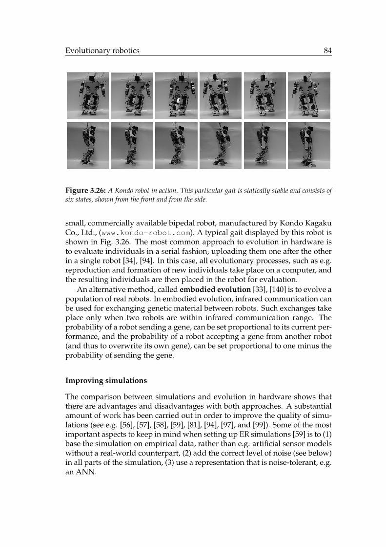
Evolutionary robotics 84
Figure 3.26: A Kondo robot in action. This particular gait is statically stable and consists ofsix states, shown from the front and from the side.
small, commercially available bipedal robot, manufactured by Kondo KagakuCo., Ltd., (www.kondo-robot.com ). A typical gait displayed by this robot isshown in Fig. 3.26. The most common approach to evolution in hardware isto evaluate individuals in a serial fashion, uploading them one after the otherin a single robot [34], [94]. In this case, all evolutionary processes, such as e.g.reproduction and formation of new individuals take place on a computer, andthe resulting individuals are then placed in the robot for evaluation.
An alternative method, called embodied evolution [33], [140] is to evolve apopulation of real robots. In embodied evolution, infrared communication canbe used for exchanging genetic material between robots. Such exchanges takeplace only when two robots are within infrared communication range. Theprobability of a robot sending a gene, can be set proportional to its current per-formance, and the probability of a robot accepting a gene from another robot(and thus to overwrite its own gene), can be set proportional to one minus theprobability of sending the gene.
Improving simulations
The comparison between simulations and evolution in hardware shows thatthere are advantages and disadvantages with both approaches. A substantialamount of work has been carried out in order to improve the quality of simu-lations (see e.g. [56], [57], [58], [59], [81], [94], [97], and [99]). Some of the mostimportant aspects to keep in mind when setting up ER simulations [59] is to (1)base the simulation on empirical data, rather than e.g. artificial sensor modelswithout a real-world counterpart, (2) add the correct level of noise (see below)in all parts of the simulation, (3) use a representation that is noise-tolerant, e.g.an ANN.

Evolutionary robotics 85
Sensors can be implemented in several different ways in ER simulations.One approach is simply to measure sensor readings on an actual robot, andstore them (e.g. in a lookup table) for later use in a simulator [86], [99]. Noisecan be added in different ways, either by slightly perturbing the measuredsensor readings, or by using actual sensor readings taken from a slightly dif-ferent position and angle than that currently held by the robot, a procedurecalled conservative position noise [86]. In this approach, sensor readingsmust be taken at many different positions, rendering the procedure quite time-consuming in all but the simplest environments. An alternative approach is toset up a physical model of the sensors, and to determine the values of themodel parameters through system identification. For example, Jakobi et al.[59] used this approach to model the IR sensors on a Khepera robot (see Ap-pendix C). They used a ray tracing technique which in which n ray tracingswere carried out (in different directions), and the resulting sensor reading wasthen modelled as
s =n∑
i=1
cosβi
(
a
d2i
+ b
)
, (3.21)
where βi is the angle at which ray i emanates from the sensor, and di is thedistance to an object along the ray. a and b were determined empirically [59].
Jakobi et al. [59] also studied the effects of noise, and found that the small-est performance difference between simulated robots and physical robots wasobtained when the noise level in simulations was set approximately equal tothe empirically determined noise level in the real world. Interestingly, it wasalso found that, in simulations with high noise levels, simulated robots couldmake use of noise to achieve good results in simulations that could not be re-produced in physical robots, showing that noise levels should not be set toohigh.
Jakobi [56], [58] has introduced a simulation procedure called minimalsimulations, which recognizes the inevitable discrepancies between the sim-ulated and real worlds. Thus, in a minimal simulation, the various aspectsof the interaction between a robot and its environment are divided into baseset aspects and implementational aspects, where the former have a physi-cal counterpart in the real world, whereas the latter do not. Thus, in a mini-mal simulation, the implementational aspects should be varied randomly fromevaluation to evaluation, thus rendering them useless to evolution, and forc-ing the EA to focus on the base set aspects. An evolved robotic brain that onlyrelies on base set aspects is called base set exclusive. In addition, a certain de-gree of variation is introduced also in the base set aspects, in order to capturethe fact that even in the base set aspects there will be discrepancies between thesimulated and real worlds. A robot that can cope also with such discrepancies,is termed base set robust.
Thus, summarizing, it is evident that the choice between evolution in sim-

Evolutionary robotics 86
ulation and evolution in hardware is a non-trivial one. Simulations have thedisadvantage of never being able to capture all aspects of the real world. How-ever, carefully designed simulations will nevertheless lead to results that canbe transferred to physical robots. Indeed, one may, perhaps, consider the re-sults obtained in a simulation as a first iteration toward the desired results.Of course, a hybrid approach can be used, in which evolution is first carriedout in simulations and then briefly continued in hardware. Miglino et al [86]report successful results from such an approach.
3.4.3 Simultaneous evolution of body and brain
The most common application of ER is to evolve the brain of a robot, adaptingit for use in a body of fixed size and shape. However, there is nothing prevent-ing the use of EAs for optimizing both the body and the brain of a robot.
Simultaneous optimization of body and brain has been considered in artifi-cial life, where Sims [119] evolved swimming, running, and hopping creatures,consisting of limbs composed of chains of block-like structures and neural net-works for moving the limbs in an oscillatory fashion. For a recent review, andalso an extension of Sims’ work, see [124]. The procedure of simultaneouslyoptimizing body and brain has been used also by several authors in the fieldof ER 5 A brief review of the topic can be found in [98].
In many such applications, see e.g. [11], [21], [24], [25], [82], [132], and[133], an artificial ontogeny (or morphogenesis) is employed, i.e. the bodyand brain of the individual are generated as the result of a developmental pro-cess, modelled on the embryological development of biological organisms, in-volving gene regulation and differential gene expression both in space andtime.6 In these cases, the encoding scheme used in the EA is, in general, muchmore complex than the simple lookup-table coding used in many other ap-plications. A simple example of an encoding scheme involving an elementof ontogeny is the grammatical encoding scheme described in Subsect. 2.7.2above.
The ability of EAs to optimize the morphology of robots opens up a plethoraof new possibilities, and reduces the severity of the problem of selecting an ap-propriate body structure a priori. As a simple example, in the pursuit-evasioncontests studied in [132] and [133], it was found that pursuers evolved forward-pointing sensors, whereas evaders evolved backward-pointing sensors. Whilethese investigations were carried out in simulation, Lichtensteiger and Eggen-
5Some authors use the term co-evolution to indicate simultaneous evolution of body andbrain. However, in order not to confuse this process with co-evolution involving different,competing species, see Subsect. 2.7.3 above, the term co-evolution should, perhaps, be avoidedin this context.
6For an introduction to gene regulation in biological systems, see e.g. [22] and [109].
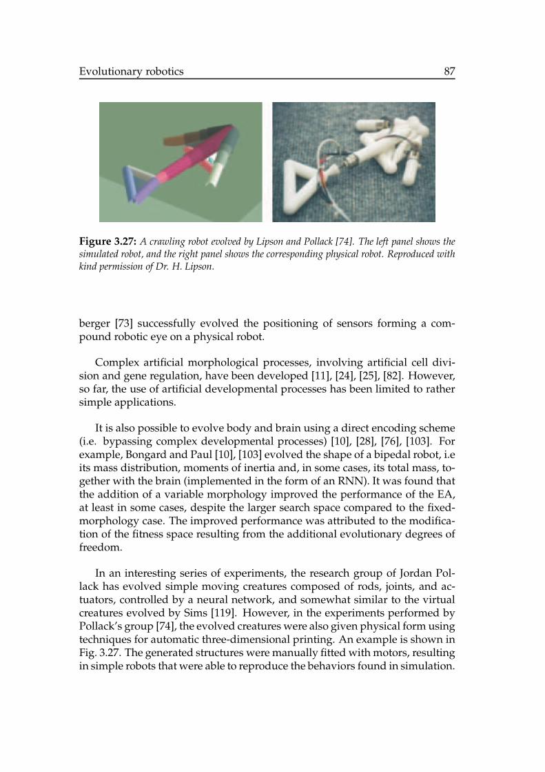
Evolutionary robotics 87
Figure 3.27: A crawling robot evolved by Lipson and Pollack [74]. The left panel shows thesimulated robot, and the right panel shows the corresponding physical robot. Reproduced withkind permission of Dr. H. Lipson.
berger [73] successfully evolved the positioning of sensors forming a com-pound robotic eye on a physical robot.
Complex artificial morphological processes, involving artificial cell divi-sion and gene regulation, have been developed [11], [24], [25], [82]. However,so far, the use of artificial developmental processes has been limited to rathersimple applications.
It is also possible to evolve body and brain using a direct encoding scheme(i.e. bypassing complex developmental processes) [10], [28], [76], [103]. Forexample, Bongard and Paul [10], [103] evolved the shape of a bipedal robot, i.eits mass distribution, moments of inertia and, in some cases, its total mass, to-gether with the brain (implemented in the form of an RNN). It was found thatthe addition of a variable morphology improved the performance of the EA,at least in some cases, despite the larger search space compared to the fixed-morphology case. The improved performance was attributed to the modifica-tion of the fitness space resulting from the additional evolutionary degrees offreedom.
In an interesting series of experiments, the research group of Jordan Pol-lack has evolved simple moving creatures composed of rods, joints, and ac-tuators, controlled by a neural network, and somewhat similar to the virtualcreatures evolved by Sims [119]. However, in the experiments performed byPollack’s group [74], the evolved creatures were also given physical form usingtechniques for automatic three-dimensional printing. An example is shown inFig. 3.27. The generated structures were manually fitted with motors, resultingin simple robots that were able to reproduce the behaviors found in simulation.
Evolutionary robotics 88
3.4.4 Simulation software
Since ER often involves the use of simulations, it is not surprising that manysimulation packages (i.e. collections of source code that can be used for gen-erating simulator for autonomous robots) and stand-alone robotic simulatorshave been developed. A few tools for ER simulations will now be introduced.
EvoRobot
The EvoRobot program is a simulator for Khepera robots, available on theworld wide web athttp://gral.ip.rm.cnr.it/evorobot/simulator.html .EvoRobot allows the user to perform various ER experiments, such as evolvingneural networks for navigation and obstacle avoidance. A variety of differentrobot parameters, such as the number and types of sensors, can be set throughthe graphical user interface. Evolution can be carried out both in simulationand using an actual Khepera robot. If simulations are used, the results can alsobe uploaded and tested in an actual Khepera robot.
Evolutionary robotics toolbox
The Evolutionary robotics toolbox (ERT) is a software package forMatlab for simulation of Khepera robots. As in the EvoRobot package, theresults from a simulation carried out in ERT can be tested on an actual Kheperarobot. The package can be downloaded fromhttp://diwww.epfl.ch/lami/team/urzelai/ertbx.html .
Webots
Webots TM is a commercially available software package [85] manufacturedby Cyberbotics (www.cyberbotics.com). Webots allows simulation of manydifferent types of robots, including Khepera, Koala (manufactured by K-team,www.k-team.com), and Aibo (manufactured by Sony, www.sony.com/aibo).As with the other robotics packages mentioned above, the results obtainedfrom a Webots simulation can be uploaded to an actual robot. In additionWebots supports, for instance, evolution of robot morphology and multi-robot simulations (such as robot soccer). Webots is equipped with an ad-vanced graphical user interface, allowing 3D rendering of simulated robots(see Fig. 3.28). Furthermore, it is possible to import 3D models deleveloped in3D modelling languages such as VRML.

Evolutionary robotics 89
Figure 3.28: A screenshot from a WebotsTM simulation of a Khepera II robot. Reproducedwith kind permission of Dr. O. Michel, Cyberbotics.
Figure 3.29: A screenshot from a simulation based on the UFLibrary software package. Thisparticular environment has been used in a project (in the author’s research group) aimed atgenerating a behavior selection system for a delivery robot (shown as a cylindrical object).
Evolutionary robotics 90
Darwin2K
Darwin2K [72] is an open source packages for robotic simulation, containingan evolutionary algorithm for ER simulations. Like Webots , Darwin2K in-cludes advanced robot models and has, among other things, been used in con-nection with research on planetary exploration robots. The Darwin2K packageis available at darwin2k.sourceforge.net .
Utility function library
The author’s research group is currently developing a general simulation pack-age, the utility function library or UFLibrary for ER applications involvingbehavioral organization using the utility function method (see Subsect. 3.3.3).The utility function library has been developed using Delphi object-orientedPascal (www.borland.com), and the first released version (v1.0.1), togetherwith a tutorial and reference manual, can now be downloaded from the in-ternet [134]. At present, the UFLibrary consists of a total of more than 12,000lines of code, divided into 51 source units, ranging from general units concern-ing e.g. the evolutionary algorithm used for the optimization of utility func-tions to more specific units such as those defining, for example, a DC motoror a laser range finder. In addition, a few basic behaviors, such as a naviga-tion behavior, an obstacle avoidance behavior etc. have been included in theUFLibrary .
UFLibrary makes possible the construction of robotic brains of arbitrarycomplexity, provided that certain guidelines (as enforced by the utility func-tion method) are followed. The functionality is provided in the form of asoftware package rather than as a stand-alone application. Although someprogramming is required to make full use of the UFLibrary , for example todefine new behaviors or to define a new stand-alone application based on thepackage, it is possible, for basic usage, to control most aspects of the simula-tions through the use of definition files in the form of simple text files. Whenimplementing an application, a minimum of two definition files are required,one for the world (arena) in which the robot is supposed to move and oper-ate, and one for the robot itself. The definition files have an object-orientedstructure, and provide an intuitive interface, even to users who have limitedprogramming experience. More detailed information concerning the use ofthe UFLibrary can be found in [134]. Also, the UFLibrary and the relateddocuments can be found on the CD accompanying this tutorial. A screenshotof a typical environment for a robotics simulation using this software is shownin Fig. 3.29.
It should be noted that a new version of the utility function method is beingdeveloped. Concurrently, a new version of the software is also being written,in which behaviors will be represented in a unified way, such that new behav-
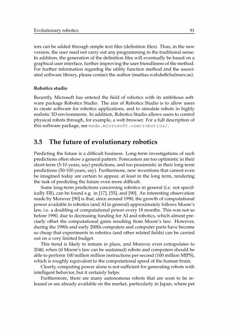
Evolutionary robotics 91
iors can be added through simple text files (definition files). Thus, in the newversion, the user need not carry out any programming in the traditional sense.In addition, the generation of the definition files will eventually be based on agraphical user interface, further improving the user friendliness of the method.For further information regardng the utility function method and the associ-ated software library, please contact the author ([email protected]).
Robotics studio
Recently, Microsoft has entered the field of robotics with its ambitious soft-ware package Robotics Studio. The aim of Robotics Studio is to allow usersto create software for robotics applications, and to simulate robots in highlyrealistic 3D environments. In addition, Robotics Studio allows users to controlphysical robots through, for example, a web browser. For a full description ofthis software package, see msdn.microsoft.com/robotics/ .
3.5 The future of evolutionary robotics
Predicting the future is a difficult business. Long-term investigations of suchpredictions often show a general pattern: Forecasters are too optimistic in theirshort-term (5-10 years, say) predictions, and too pessimistic in their long-termpredictions (50-100 years, say). Furthermore, new inventions that cannot evenbe imagined today are certain to appear, at least in the long term, renderingthe task of predicting the future even more difficult.
Some long-term predictions concerning robotics in general (i.e. not specif-ically ER), can be found e.g. in [17], [55], and [90]. An interesting observationmade by Moravec [90] is that, since around 1990, the growth of computationalpower available to robotics (and AI in general) approximately follows Moore’slaw, i.e. a doubling of computational power every 18 months. This was not sobefore 1990, due to decreasing funding for AI and robotics, which almost pre-cisely offset the computational gains resulting from Moore’s law. However,during the 1990s and early 2000s computers and computer parts have becomeso cheap that experiments in robotics (and other related fields) can be carriedout on a very limited budget.
This trend is likely to remain in place, and Moravec even extrapolates to2040, when (if Moore’s law can be sustained) robots and computers should beable to perform 100 million million instructions per second (100 million MIPS),which is roughly equivalent to the computational speed of the human brain.
Clearly, computing power alone is not sufficient for generating robots withintelligent behavior, but it certainly helps.
Furthermore, there are many autonomous robots that are soon to be re-leased or are already available on the market, particularly in Japan, where pet

Evolutionary robotics 92
Figure 3.30: The PaPeRo personal robot. c© NEC. Reproduced with kind permission of theNEC corporation.
robots such as AIBO, and humanoid robots such as ASIMO, have had greatsuccess. The fact that robots such as AIBO are mass produced is also impor-tant: The possibility of making profits from the construction of autonomousrobots is, of course, an essential driving force in their development.
So far, the capabilities of commercially available robots are quite limited,even though they are important precursors for more advanced robots. In ad-dition to entertainment robots such as AIBO, commercially available robotsinclude lawn moving robots, vacuuming robots, and robots for autonomoustransportation in hospitals. There are also prototypes for general-purposehousehold robots, such as the NEC PaPeRo robot shown in Fig. 3.30.
Returning now the ER, some general trends can be observed. Note thatthe following paragraphs reflect the author’s view. For an alternative (but notnecessarily conflicting) view of the short- to intermediate-term future of ER,see e.g. [37].
First of all, a result of the increasing complexity of robotic brains is to re-duce further the possibility of generating such systems by hand. Thus, if any-thing, ER is likely to become more useful as complexity grows. This can beseen e.g. in recent EA-based methods for behavioral organization [131]. In-deed, behavioral organization is of paramount importance in for ER to be ableto deliver robots with the capabilities needed for autonomous operation in re-alistic environments. Current research efforts in this field show that EA-basedmethods indeed are able to generate complex robotic brains, with a minimum

Evolutionary robotics 93
of hand-coding by the experimenter [107].Furthermore, it is likely that the EAs used for ER (and also for other ap-
plications) will become increasingly sophisticated incorporating, among otherthings, artificial gene regulation and ontogeny, as described in Subsects. 2.7.2and 3.4.3, to a greater degree than today. Indeed, the march towards morecomplex EAs is inspired, in part, by the rapid developments in molecular biol-ogy [22] and bioinformatics [12]. In particular, the advent of massively parallelgene expression measurements using microarray techniques [110] has led to arapid increase in the amount of biological data available, and the cooperationof biology and computer science in bioinformatics continues to deliver newinformation concerning the organization and function of biological systems,information that is likely to be assimilated also in EAs.
In addition, the simultaneous evolution of body and brain is likely to be-come increasingly important in ER. In biological systems, brains and bodieshave, of course, evolved together, and form an integrated system. Thus, de-spite the increasing complexity introduced by variable morphologies, it is pos-sible that simultaneous evolution of body and brain may, in fact, speed upevolution [10], [103].
Finally, it is likely that there will appear many new multi-robot applica-tions, in which the evolutionary process must also take into account the com-munication between robots [80], [144], as well as the communication betweenrobots and people [39]. A particularly interesting topic is the emergence ofcomplex, self-organized collective behavior from simple, local interactions,akin to stigmergy [125] in social insects such as ants and termites.
To summarize, it is evident that the influence from molecular biology, ge-netics, and ethology will continue to play an important role in ER and in thenear future, increasingly advanced robots, based in whole or in part on ER,will in all probability appear on the market, ready and able to help peoplewith a variety of tedious and dangerous tasks.

Appendix A: Artificial neuralnetworks
The aim of this appendix is to give a very brief introduction to neural net-works, introducing only those parts of this vast topic that will be used inthis tutorial. For a more thorough introduction see [48]. Artificial neural net-works (ANNs) are computational structures (loosely) based on the structureand function of biological neural networks that constitute the brains of ani-mals. Basically, an ANN is a set of interconnected elements, called neurons.
Neurons
The main computational element in neural networks, the neuron, is illustratedin Fig. A1. In essence, a neuron receives weighted inputs, either from otherneurons (or from the neuron itself, in some networks, see below), or from in-put elements, sums these input, adds a bias to form an internal signal, andproduces an output by passing the internal signal through a squashing func-tion. ANNs may operate either in discrete time or continuous time. In theformer case, the output of neuron i in a network, denoted xi is computed as
xi = σ
(
∑
j
wijzj + bi
)
, (A1)
where wij are the connection weights, zj the input signals to the neuron andbi is the bias. In the continuous case, the output at time x(t) is typically givenby the differential equation
τixi(t) + xi(t) = σ
(
∑
j
wijzj + bi
)
, (A2)
where τi are time constants. Typically, the zj are inputs from other neurons(or even the neuron i itself), so that the equations for different neurons arejoined into a set of coupled non-linear differential equations. Other equationsare also possible, of course. In any case, the neuron equations presented above
94
Appendix A: Artificial neural networks 95
wn
w2
w1
b
S s
Figure A1: An artificial neuron. First, the input signals, multiplied by the weights, areadded. Next, the bias b is added, and the output is computed using the squashing function σ.
represent very a strong simplification of the very intricate method of operationof actual biological neurons. The squashing function can be chosen in variousdifferent ways. Two common choices are the logistic function
σ(z) =1
1 + e−cz, (A3)
which restricts the output to the range [0, 1], and the hyperbolic tangent
σ(z) = tanh cz, (A4)
which restricts the output to [−1, 1]. In both functions, c is a positive constant,which determines the steepness of the squashing function. If c is set to a verylarge value, σ(z) approaches a step function.
Network types
The two main types of neural networks are feedforward neural networks(FFNNs) and recurrent neural networks (RNNs). In the former, neurons arearranged in layers, and signals flow from the input layer to the first hiddenlayer, from the first hidden layer to the second hidden layer etc. until the out-put layer is reached. By contrast, in RNNs, any neuron may be connected toany other neuron. RNNs often operate in continuous time, using Eq. (A2) torepresent neurons. The difference between FFNNs and RNNs is illustrated inFig. A2. For the FFNN, shown in the left panel of the figure, the input sig-nals are denoted Ij, the neurons in the middle layer xH, and the neurons inthe output layer xO. Assuming the network operates in discrete time, which iscommon in FFNNs, the corresponding network equations will be
xHi = σ
(
∑
j
wIHij Ij + bi
)
, (A5)

Appendix A: Artificial neural networks 96
Figure A2: The left panel shows a feedforward neural network (FFNN), whereas the rightpanel shows a recurrent neural network (RNN), in which feedback connections are present.
where wIHij are the weights connecting input element j to neuron i in the hid-
den layer, and
xOi = σ
(
∑
j
wHOij xH
j + bi
)
, (A6)
where wHOij are the weights connecting the hidden layer to the output layer.
Note that the first (leftmost) layer (the input layer) in the FFNN does not con-sist of neurons: the elements in this layer, indicated by squares to distinguishthem from neurons that are indicated by circles, simply serve to distribute theinput signals to the neurons in the hidden layer. No squashing function is as-sociated with the elements in the input layer. In general, the term units can beused to refer either to input elements or to neurons.
An RNN is shown in the right panel of Fig. A2. Here, neurons are not(necessarily) arranged in layers, and the output of a typical neuron is given by
τixi(t) + xi(t) = σ
(
∑
j
wijxj(t) +∑
j
wIijIj(t) + bi
)
, (A7)
wherewij are the weights connecting neurons to each other, andwIij are weights
connecting input j to neuron i. Again, the inputs are shown as squares in thefigure, and the neurons are shown as circles. Since RNN are not arranged inlayers, there are no natural output neurons. Instead, some neurons are sim-ply selected to be the output neurons. The number of such neurons varies, ofcourse, from problem to problem.
Training an ANN
In a neural network, the computation is intertwined with the structure of thenetwork (i.e. the number of neurons, and their connections to each other). Ifthe structure is changed, the computation changes as well. Thus, in order for anetwork to perform a given type of computation, both the number of neurons
Appendix A: Artificial neural networks 97
and the network weights must be set to appropriate values, a process knownas training. There are various algorithms for training neural networks. Themost common algorithm, applicable to FFNNs, is the backpropagation algo-rithm [48]. This training algorithm requires that the reward is immediate: forany input signal, it must be possible to judge directly the quality of the outputby means of an error function. For this reason, backpropagation belongs to afamily of training algorithms known as supervised training algorithms. Inci-dentally, it can be mentioned that the error function must be differentiable forbackpropagation to function properly. No such restrictions are required in thecase of ANN optimization by means of EAs.
However, supervised training methods are rarely applicable in ER, sinceimmediate rewards do not normally occur. Instead, the reward (if any) for agiven action generally occurs long after the action was taken. In addition back-propagation, as indeed many other methods developed in the neural networkliterature, require that the structure of the ANN be specified in advance. In ERit is generally impossible to specify the best structure of a ANN-based roboticbrain beforehand. Thus, for these reasons, EAs are often the method of choicewhen generating ANNs in ER and, in this tutorial, only EA-based generationof ANNs will be considered.

Appendix B: Finite-state machines
In addition to neural networks (see Appendix A), finite-state machines aresometimes used for representing robotic brains in connection with ER.
A finite-state machine [38] (hereafter FSM) consists, as the name implies,of a finite number of states and conditional transitions between those states.At every time step, an FSM reads an input symbol, and produces an outputsymbol as it jumps to the next target state.
In FSMs, the input and output symbols are taken from two discrete alpha-bets. Commonly, the input alphabet, i.e. the symbols received by the FSM, isthe same as the output alphabet, i.e. the symbols generated by the FSM.A simple FSM is shown in Fig. B1. In this case, the input and output alphabetsboth consist of the symbols 0 and 1, and the input-output mapping is shownin the right panel of the figure. Unlike FFNN (see Appendix A), FSMs can beequipped with a dynamic memory of previous events, and can thus be usede.g. to generate robotic brains that reach beyond the realm of purely reactivebehaviors.
FSMs, as introduced above, operate with discrete variables, however, andare therefore not always suitable in connection with autonomous robots, which,of course, operate in continuous time. A useful extension to FSMs are gener-alized finite-state machines (GFSMs) [137]. Like ordinary FSMs, GFSMs con-sist of a finite number of states and transitional conditions between the states.However, in GFSMs, each state consists of a specific setting of (some of) thevariables of the system under study. For example, in the case of a Kheperarobot (see Appendix C), the variables specified in a state may be the speeds ofthe two motors.
From each state i, there are Mi conditional transitions to other states. In thecase of autonomous robots, the conditions often involve the sensor readings,but other variables can also be used. The conditions can, in principle, be arbi-trarily complex, and are thus not restricted to a particular alphabet, as in FSMs.If a condition is satisfied, the GFSM immediately jumps to the correspondingtarget state. No particular action is associated with the jump from one state toanother. If none of the conditions are satisfied, the GFSM remains in the samestate, as indicated for state 1 in Fig. B2.
Thus, in GFSMs, each state is associated with some specific variable setting,
98

Appendix B: Finite-state machines 99
0/1
1/0
0/11/1
0/0
1/1 1/1
0/1
state input output state(before) (after)
1 0 1 22 1 0 11 1 1 33 0 0 44 1 1 11 0 1 2
1 2
3 4
. . .
. . .
. . .
. . .
Figure B1: A simple finite-state machine.
State 1
State 2
State j
. . .
Condition 1 Condition 2 Condition M1. . .
. . .State N
Figure B2: A GFSM. There are N states and, for each state i, there are Mi conditionaltransitions (which differ from state to state). Only one conditional transition is shown in thefigure, namely from state 1 to state j.
whereas in ordinary FSMs it is the state transitions that are associated withthe actions. This reduces the number of possible variable settings for GFSMscompared to FSMs for a given state machine size since, normally, there aremore transitions than states. However, it also makes the architecture moretransparent and easy to interpret.

Appendix C: The Khepera robot
During the last few decades, a large number of autonomous robots have beendeveloped, both by robotics researchers and, more recently, by companies suchas Sony, Honda etc. In this appendix, the properties of one commerciallyavailable robot, namely the Khepera robot developed by K-team (www.k-team.com) will be described briefly. The Khepera robot has, for many years,been a popular tool in ER, due to the facts that it is very compact and light (andthus easy to transport), easy to program, and equipped with basic sensory ca-pabilities. In addition, the fact that the robot is so widely used, as evidencedby the many examples in Chapter 3, facilitates the comparison of the resultsobtained by different research groups. The also exists several simulators forKhepera (see Subsect. 3.4.4), some of which allow evolved robotic brains to beuploaded directly onto an actual Khepera robot.
Khepera is a small differentially steered robot, equipped with two wheelsand eight infrared sensors in the standard configuration. Several additionalmodules, such as linear vision arrays and gripper arms, can be added to thestandard Khepera configuration. Two versions of Khepera exist: the originalversion (called Khepera I in the remainder of this appendix) with a diameterof around 55mm, and an improved version (Khepera II), with a diameter ofaround 70mm. The weight of the robot is approximately 80g (Khepera II).
Pictures of Khepera I and Khepera II are shown in Fig. C1. The robotis equipped with a processor from the Motorola 68K family, and has a RAMmemory of 256 Kb (Khepera I) or 512 Kb (Khepera II).
The robot can be programmed in C, and the communication between thecomputer and the robot is carried out via a serial cable. Once a program hasbeen downloaded into a Khepera robot, the cable can be removed and therobot is then fully autonomous. Each Khepera robot carries four rechargeableNiCd batteries, which allow the robot to operate for around 45 minutes (Khep-era I) to one hour (Khepera II). However, for longer operation, the robot canbe powered via the serial cable.
The robot is equipped with two DC motors, one on each side. The low-level control of both motors is handled by PID controllers, which allow theuser to set either a speed or a position, without worrying about the details ofthe motor control. The top speed of the robot is around 1 m/s. It is possible
100

Appendix C: The Khepera robot 101
Figure C1: The Khepera family: Khepera I (left panel) and Khepera II (right panel). Photosby the author.
2 3
1 4
0 5
7 6
Figure C2: A schematic view of the Khepera robot. The infrared sensors are numbered from0 to 7.
also to override the motor controllers and take more direct control over themotion of the robot.
As shown in the schematic view of the robot (Fig. C2), the robot has eightinfrared proximity sensors numbered from 0 (just in front of the left wheel inFig. C2) to 7 (behind the left wheel). The sensors can be used in two modes,either to measure the ambient light levels (using only the reception of infraredlight) or to measure the light reflected by objects surrounding the robot (byemitting infrared light and measuring the reflection). The sensors update theirreadings every 20 ms, allowing high resolution (in time) of the measurements.The readings for each sensor are integer values between 0 and 1023.
The sensor range for measurement of reflected light varies with the reflec-tivity of the object in question, but is around 20–50 mm (i.e. of the same orderof magnitude as the size of the robot itself) for Khepera I and up to 100 mmfor Khepera II. It should be noted that the Khepera is rather sensitive to theamount of ambient light present, and can easily be blinded if a strong lightsource is suddenly turned on.

Bibliographical notes
These tutorial notes are, of course, intended as an introduction to the ER liter-ature. However, the reader should also consult the original sources, given inthe reference list below. Because of the length of the reference list, however,readers who are new to the field of ER may be helped by some guidance, es-pecially since many of the references do not directly deal with ER but insteadwith closely related topics, such as BBR, ANNs etc.
Thus, in addition to these tutorial notes, the reader is recommended to be-gin by considering the book on evolutionary robotics by Nolfi and Floreano[97], as well as review papers such as [46], [47], [83], and [99]. It is also rec-ommended to read introductory texts on behavior-based robotics [3], ethology[30], and molecular biology [22], since all these fields have a strong influenceon research in ER.
Furthermore, despite its length, the reference list below is only a partial(and probably biased) sample of the many papers available in ER. Thus, thereader is recommended to consult journals in which ER-based research ap-pears, e.g. Adaptive Behavior, Artificial Life, Evolutionary Computation, IEEETransactions on Evolutionary Computation, IEEE Transactions on Systems,Man, and Cybernetics, and Robotics and Autonomous Systems, as well asthe proceedings of the many conferences in which ER is often featured, e.g.Simulation of Adaptive Behavior (SAB), Artificial life (ALIFE), EvolutionaryRobotics (ER), Genetic and Evolutionary Computation (GECCO), IntelligentRobots and Systems (IROS), Robotics and Automation (ICRA), and Systems,Man, and Cybernetics (SMC). The author maintains a regularly updated list ofconferences in ER and related fields, which is available athttp://www.me.chalmers.se/˜mwahde/ConferenceList.ph p
102
Bibliography
[1] Andreasson, N., Evgrafov, A., and Patriksson, M. An introduction to con-tinuous optimization: foundations and fundamental algorithms, Studentlitter-atur, 2005
[2] Arakawa, T and Fukuda, T. Natural motion trajectory generation of bipedlocomotion using genetic algorithm through energy optimization, In: Proc. ofthe 1996 IEEE Int. Conf. on Systems, Man, and Cybernetics, pp. 1495-1500, 1996
[3] Arkin, R.C. Behavior-based robotics, MIT Press, 1998
[4] Back, T., Fogel, D.B., and Michalewicz, Z. (Eds.), Handbook of Evolution-ary Computation, Institute of Physics Publishing and Oxford UniversityPress, 1997
[5] Back, T., Hoffmeister, F., and Schwefel, H.-P. A Survey of Evolution Strate-gies, In: Proc. of the 4th Int. Conf. on Genetic Algorithms, Morgan Kauf-mann Publishers, pp. 2-9, 1991
[6] Banzhaf, W., Nordin, P., Keller, R.E., and Francone, F.D. Genetic Program-ming - An Introduction, Morgan Kaufmann Publishers, 1998
[7] Bassett, J.K. and De Jong, K.A. Evolving Behaviors for Cooperating Agents,In: Proc. of the 12th Int. Symp. on Methodologies for Intelligent Systems,pp. 157-165, 2000
[8] Belew, R. K. and Mitchell, M. Adaptive Individuals in Evolving Populations:Models and Algorithms, Santa Fe Institute Studies in the Science of Com-plexity, 26, pp. 1-22, 1996
[9] Blumberg, B.M. Action-selection in Hamsterdam: lessons from ethology. In:From Animals to Animats 3: Proc. of the 3rd Int. Conf. on Simulation ofAdaptive Behavior (SAB94), MIT Press, 1994
[10] Bongard, J.C. and Paul, C. Making Evolution an Offer It Can’t Refuse: Mor-phology and the Extradimensional Bypass, Lecture Notes in Computer Sci-ence, 2159, pp. 401-412, 2001
103

Bibliography 104
[11] Bongard, J.C. and Pfeifer, R. Evolving Complete Agents using Artificial On-togeny, In: Morpho-functional Machines: The New Species, Springer-Verlag, 237-258, 2003
[12] Bower, J.M. and Bolouri, H. (Eds.) Computational Modeling of Genetic andBiochemical Networks, MIT Press, 2001
[13] Brameier, M. On linear genetic programming, PhD thesis, Dortmund Uni-versity, Dortmund, Germany, 2003
[14] Brooks, R.A. A Robust Layered Control System for a Mobile Robot, IEEE Jour-nal of Robotics and Automation, RA-2, No. 1, pp. 14-23, 1986
[15] Brooks, R.A. Artificial life and real robots, In: Proc. of the first Europeanconference on artificial life (ECAL91), MIT Press, pp. 3-10, 1992
[16] Brooks, R.A. Prospects for human level intelligence for humanoid robots,In: Proc. of the First International Conference on Humanoid Robots(HURO-96)
[17] Brooks, R.A. Robot: The Future of Flesh and Machines, Penguin Press, Pa-perback Ed., 2003
[18] Cheng, M.-Y. and Lin, C.-S. Genetic algorithm for control design of bipedlocomotion, In: Proc. of the IEEE Int. Conf. on Robotics and Automation,pp. 1315-1320, 1995
[19] Cliff, D., Harvey, I., and Husbands, P. Explorations in EvolutionaryRobotics, Adaptive Behavior 2:1, pp. 73-110, 1993
[20] Cliff, D., Husbands, P., and Harvey, I. Evolving visually guided robots In:Proc. of the 2nd Int. Conf. on Simulation of Adaptive Behavior (SAB92),MIT Press/Bradford books pp 374–383, 1993
[21] Cliff, D. and Miller, G.F. Co-evolution of pursuit and evasion II: Simulationmethods and results, in Proc. of the 4th Int. Conf. on the Simulation ofAdaptive Behavior (SAB96), MIT Press, pp. 506-515, 1996
[22] Davidson, E.H. Genomic Regulatory Systems - Development and Evolution,Academic Press, 2001
[23] Dawkins, R. Climbining Mount Improbable, Penguin books, 1997
[24] Dellaert, F. and Beer, R.D. A Developmental Model for the Evolution of Com-plete Autonomous Agents, In: Proc. of the 4th Int. Conf. on Simulation ofAdaptive Behavior (SAB96), MIT Press, pp. 393-401, 1996

Bibliography 105
[25] Dellaert, F. and Beer, R.D. Toward an evolvable model of development forautonomous agent synthesis, In: Proc. of the 4th Int. Conf. on Artificial Life,MIT Press, 1994
[26] Dorigo, M. and Stutzle, T. Ant Colony Optimization, MIT Press, 2004
[27] Duckett, T. A Genetic Algorithm for Simultaneous Localization and Mapping,In: Proc. of the 2003 Int. Conf. on Robotics and Automation (ICRA2003),pp. 434-439, 2003
[28] Endo, K., Maeno, T., and Kitano, H. Co-evolution of Morphology and Walk-ing Pattern of Biped Humanoid Robot using Evolutionary Computation - Evo-lutionary Designing Method and its Evaluation, In: Proc. of the IEEE/RSJInt. Conf. on Intelligent Robots and Systems, pp. 340-345, 2003
[29] Erinc, G. and Carpin, S. A genetic algorithm for nonholonomic motion plan-ning, In: Proc. of the IEEE 2007 Int. Conf. on Robotics and Automation(ICRA2007), pp. 1843-1849, 2007
[30] McFarland, D. Animal Behaviour, Addison-Wesley, 1999
[31] McFarland, D., and Bosser, T. Intelligent Behavior in Animals and Robots,MIT Press, 1993
[32] McFarland, D. and Spier, E. Basic cycles, utility, and opportunism in self-sufficient robots, Robots and Autonomous Systems, 20, pp. 179-190, 1997
[33] Ficici, S.G., Watson, R.A., and Pollack, J.B. Embodied Evolution: A Re-sponse to Challenges in Evolutionary Robotics, In: Proc. of the 8th EuropeanWorkshop on Learning Robots, pp. 14-22, 1999
[34] Floreano, D. and Mondada, F. Evolution of homing navigation in a real mo-bile robot, IEEE Transactions on Systems, Man, and Cybernetics, Part B,26, pp. 396–407, 1996
[35] Floreano, D. and Mondada, F. Evolution of plastic neurocontrollers for sit-uated agents, In: Proc. of the 4th Int. Conf. on Simulation of AdaptiveBehavior (SAB96), pp. 402-410, 1996
[36] Floreano, D., Nolfi, S., and Mondada, F. Competitive Co-EvolutionaryRobotics: From Theory to Practice, In: Proc. of the 5th Int. Conf. on Sim-ulation of Adaptive Behavior (SAB98), pp. 515-524, 1998
[37] Floreano, D. and Urzelai, J. Evolutionary Robots: The Next Generation, In:Proc. of the 7th Int. Symp. on Evolutionary Robotics (ER2000), 2000
[38] Fogel, L.J. Intelligence through Simulated Evolution, Wiley, 1999

Bibliography 106
[39] Fong, T., Nourbakhsh, I., and Dautenhahn, K. A survey of socially interac-tive robots, Robotics and Autonomous Systems 42, pp. 143-166, 2003
[40] Fujimoto, Y. and Kawamura, A. Simulation of an autonomous biped walkingrobot including environmental force interaction, IEEE Robotics and Automa-tion Magazine 5, No. 2, pp. 33-42, 1998
[41] Furusho, J., Akihito, S., Masamichi, S., and Eichi, K. Realization of bouncegait in a quadruped robot with articular-joint-type legs In: Proc. of the IEEEInt. Conf. on Robotics and Automation, pp. 697-702, 1995
[42] Furusho, J., Masubuchi, M. Control of a dynamical biped locomotion systemfor steady walking, Journal of Dynamical Systems, Measurements, andControl, 108, pp. 111-118, 1986
[43] Geisler, T. and Manikas, T.W. Autonomous robot navigation system using anovel value encoded genetic algorithm, In: Proc. of the 45th IEEE MidwestSymp. on Circuits and Systems, 2002
[44] Gomez, F. and Miikkulainen, R.. Incremental evolution of complex generalbehavior, Adaptive Behavior, 5, pp. 317–342, 1997
[45] Gruau, F. Automatic Definition of Modular Neural Networks, Adaptive Be-havior 3:2, pp. 151-183, 1994
[46] Harvey, I., Husbands, P., and Cliff, D. Issues in Evolutionary Robotics, In:From Animals to Animats II: Proc. of the 2nd Int. Conf. on Simulation ofAdaptive Behavior (SAB92), pp. 364-373, 1992
[47] Harvey, I., Husbands, P., Cliff, D., Thompson, A., and Jakobi, N. Evolu-tionary robotics: the Sussex approach, Robotics and Autonomous Systems,20, No 2-4, pp. 205-224, 1997
[48] Haykin, S. Neural networks - A comprehensive foundation, Prentice-Hall,1994
[49] Hillis, W.D., Co-evolving parasites improve simulated evolution as an opti-mization procedure, Physica D, 42, pp. 228-234, 1990
[50] Hirai, K., Hirose, M., Haikawa, Y., and Takenaka, T. The development ofthe Honda humanoid robot, In: Proc. of the IEEE Int. Conf. on Robotics andAutomation, 2, pp. 1321-1326, 1998
[51] Holland, J. H. Adaptation in Natural and Artificial systems, University ofMichigan Press, 1975 (2nd Ed.: MIT Press, 1992)
Bibliography 107
[52] Hornby, G., Fujita, M., Takamura, S., Yamamoto, T., and Hanagata, O.Autonomous evolution of gaits with the Sony quadruped robot, In: Proc. of theGenetic and Evolutionary Computation Conference, Morgan Kaufmann,vol. 2, pp. 1297-1304, 1999
[53] Hornby, G., Takamura, S., Yokono, J., Hanagata, O., Yamamoto, T., andFujita, M. Evolving robust gaits with aibo In: Proc. of the IEEE Int. Conf. onRobotics and Automation, pp. 3040-3045, 2000
[54] Huang, Q., Nakamura, Y., Inamura, T. Humanoids walk with feedforwarddynamic pattern and feedback sensory reflection, In: Proc. of the IEEE Int.Conf. on Robotics and Automation, pp. 4220-4225, 2001
[55] Inoue, H. and Hirukawa, H. Explorations of Humanoid Robot Applications,In: Proc. of the IEEE-RAS Int. Conf. on Humanoid Robots, pp. 497-499,2001
[56] Jakobi, N. Minimal Simulations for Evolutionary Robotics, PhD thesis,School of Cognitive and Computing Sciences, University of Sussex, 1998
[57] Jakobi, N. Running across the reality gap: Octopod locomotion evolved in aminimal simulation. In: Proceedings of Evorobot, Springer Verlag, 1998
[58] Jakobi, N. The Minimal Simulation Approach to Evolutionary Robotics, In:Evolutionary Robotics - From Intelligent Robots to Artificial Life, proc.of ER98, AAI Books, 1998
[59] Jakobi, N., Husbands, P., and Harvey, I. Noise and the reality gap: The useof simulation in evolutionary robotics, Lecture Notes in Computer Science,929, pp. 704-720, 1995
[60] Katagami, D. and Yamada, S. Teachers’s Load and Timing of Teaching basedon Interactive Evolutionary Robotics, In: Proc. of the 2003 IEEE Int. Symp.on Computational Intelligence in Robotics and Automation, 2003
[61] Kato, I. and Tsuiki, H. The hydraulically powered walking machine with ahigh carrying capacity In: 4th Int. Symp. on External Control of HumanExtremities. Yugoslav Committee for Electronics and Automation, pp.410-421, 1972
[62] Kennedy, J. and Eberhart, R. Particle swarm optimization, In: Proc. of theIEEE Int. Conf. on Neural Networks, Piscataway, NJ, pp. 1942-1948, 1995
[63] Keymeulen, D., Iwata, M., Kuniyoshi, Y., and Higuchi, T. Comparisonbetween an Off-line Model-free and an On-line Model-based Evolution appliedto a Robotics Navigation System using Evolvable Hardware, Proc. of the 6thInt. Conf. on Artificial Life, pp. 199-208, 1998
Bibliography 108
[64] Khatib, O. Real-time obstacle avoidance for manipulators and mobile robots,Int. J. of Robotics Research, 5:1, pp. 90-98, 1986
[65] Kim, K.-J. and Cho, S.-B. Robot action selection for higher behaviors withCAM-Brain modules, In: Int. Symp. on Robotics, pp. 1623-1628, 2001
[66] Kitano, H. Designing neural networks using genetic algorithms with graphgeneration system, Complex Systems 4, pp. 461-476, 1990
[67] Koza, J.R. Evolution of Subsumption Using Genetic Programming, In: Proc.of the First European Conf. on Artificial Life, MIT Press, pp. 110-119,1992
[68] Koza, J.R. Genetic Programming: On the Programming of Computers byMeans of Natural Selection, MIT Press, 1992
[69] Langton, C. (Ed.) Artificial Life - An Overview, MIT Press, 1997
[70] Lazarus, C. and Hu, H. Evolving goalkeeper behaviours for simulated soccercompetition, In: Proceedings of the 3rd IASTED International Conferenceon Artificial Intelligence and Applications (AIA 2003), 2003
[71] Lee, W.-P., Hallam, J., Lund, H.H. Applying Genetic Programming to EvolveBehavior Primitives and Arbitrators for Mobile Robots, In: Proc. of the 4th Int.Conf. on Evolutionary Computation, 1997
[72] Leger, C. Darwin2K: An Evolutionary Approach to Automated Design forRobotics, Kluwer Academic Publishers, 2000
[73] Lichtensteiger, L. and Eggenberger, P. Evolving the Morphology of a Com-pound Eye on a Robot, In: Proc. of the Third European Workshop on Ad-vanced Mobile Robots (Eurobot99), pp. 127-134, 1999
[74] Lipson, H. and Pollack, J.B. Automatic design and manufacture of roboticlifeforms, Nature, 406, pp. 974-978, 2000
[75] Luke, S., Hohn, C., Farris, J., Jackson, G., and Hendler, J. Co-evolvingSoccer Softbot Team Coordination with Genetic Programming, In: RoboCup97: Robot Soccer World Cup, Springer Verlag, pp. 398-411, 1997
[76] Lund, H.H., Hallam, J., and Lee, W. Evolving robot morphology, In: Proc.of the IEEE 4th Int. Conf. on Evolutionary Computation, IEEE Press, pp.197-202, 1997
[77] Lund, H.H., Miglino, O., Pagliarini, L., Billard, A., and Ijspeert, A. Evo-lutionary Robotics - A Children’s Game, In: Proc. of the 5th IEEE Int. Conf.on Evolutionary Computation, IEEE Press, pp. 154-158, 1998

Bibliography 109
[78] Maes, P. How to do the right thing, Connection Sci. J., 1, No. 3, pp. 291-323,1989
[79] Maes, P. Modeling Adaptive Autonomous Agent, Artificial Life, 1:1-2, pp.135-162, 1994
[80] Mataric, M. Learning to Behave Socially, In: Proc. of the 3rd Int. Conf. onSimulation of Adaptive Behavior (SAB94), pp. 453-462, 1994
[81] Mataric, M. and Cliff, D. Challenges in evolving controllers for physicalrobots, Robotics and Autonomous Systems, 19, No. 1, pp. 67-83, 1996
[82] Mautner, C. and Belew R. K. Evolving Robot Morphology and Control, In:Proc. of Artificial Life and Robotics 1999 (AROB99), 1999
[83] Meyer, J.-A. Evolutionary Approaches to Neural Control in Mobile Robots, In:Proc. of the IEEE Int. Conf. on Systems, Man, and Cybernetics, 1998
[84] Michalewicz, Z. Genetic Algorithms + Data Structures = Evolution Pro-grams, 3rd Ed., Springer, 1996
[85] Michel, O. WebotsTM: Professional Mobile Robot Simulation, Int. J. of Ad-vanced Robotic Systems, 1:1, pp. 39-42, 2004
[86] Miglino, O., Lund, H.H., and Nolfi, S. Evolving Mobile Robots in Simulatedand Real Environments, Artificial Life, 2, pp. 417-434, 1996
[87] Miglino, O., Nafasi, C., and Taylor, C. Selection for Wandering Behavior ina Small Robot, Tech. Rep. UCLA-CRSP-94-01, Department of CognitiveScience, UCLA, 1994.
[88] Mitchell, M. An Introduction to Genetic Algorithms, MIT Press, 1996
[89] Miwa, H., Takanobu, H. and Takanishi, A. Development of a human-likehead robot we-3rv with various robot personalities, In: Proc. of the IEEE-RASInternational Conference on Humanoid Robots, pp. 117-124, 2001
[90] Moravec, H. Robot: Mere Machine to Transcendent Mind, Oxford Univer-sity Press, 1999
[91] Moriarty, D. E. and Miikkulainen, R. Evolving obstacle avoidance behaviorin a robot arm. In: From Animals to Animats: Proc. of the 4th Int. Conf. onSimulation of Adaptive Behavior (SAB96), MIT Press, pp. 468-475, 1996
[92] Nelson, A.L., Grant, E., Galeotti, J.M., and Rhody, S. Maze exploration be-haviors using an integrated evolutionary robotics environment, Robotics andAutonomous Systems 46, pp. 159-173, 2004

Bibliography 110
[93] Nelson, A.L., Grant, E., Henderson, T.C. Evolution of neural controllers forcompetitive game playing with teams of mobile robots, Robotics and Autono-mous Systems 46, pp. 135-150, 2004
[94] Nolfi, S. Evolving non-trivial behaviors on real robots: A garbage collectingrobot. Robotics and Autonomous Systems, 22, pp. 187–198, 1997
[95] Nolfi, S. Power and Limits of Reactive Agents. Neurocomputing, 42, pp.119-145, 2002
[96] Nolfi, S. and Floreano, D. Learning and evolution Autonomous Robots,7:1, pp. 89-113, 1998
[97] Nolfi, S. and Floreano, D. Evolutionary robotics, MIT Press, 2000.
[98] Nolfi, S. and Floreano, D. Synthesis of autonomous robots through evolution,Trends in Cognitive Science, 6:1, pp. 31-36, 2002
[99] Nolfi, S., Floreano, D., Miglino, O., and Mondada, F. How to evolve au-tonomous robots: Different approaches in evolutionary robotics, In: ArtificialLife IV, pp. 190–197, 1994.
[100] Nolfi, S. and Marocco, D. Evolving Robots Able to Visually DiscriminateBetween Objects with Different Size, International Journal of Robotics andAutomation (17) 4, pp. 163-170, 2002
[101] Ostergaard, E.H. and Lund, H.H. Co-Evolving Complex Robot Behavior, In:Proc. of the 5th Int. Conf. on Evolvable Systems (ICES2003), pp. 308-319,Springer Verlag, 2003
[102] Parker, G.B., Georgescu, R., and Northcutt, K. Continuous Power Supplyfor a Robot Colony, Proceedings of the World Automation Congress, 2004
[103] Paul, C. and Bongard, J.C. The Road Less Travelled: Morphology in the Opti-mization of Biped Robot Locomotion, In: Proc. of the IEEE/RSJ Int. Conf. onIntelligent Robots and Systems (IROS2001), IEEE Press, 1, pp. 226-232,2001
[104] Pettersson, J. Generating Motor Behaviors for Bipedal Robots Using Biolog-ically Inspired Computation Methods, Licentiate Thesis, Chalmers Univer-sity of Technology, 2003
[105] Pettersson, J., Hartono, P., and Wahde, M. A behavior module for odometrycalibration in autonomous robots, Submitted to AMiRE2007.
[106] Pettersson, J., Sandholt, H., and Wahde, M. A flexible evolutionary methodfor the generation and implementation of behaviors in humanoid robots In:Proc. of the IEEE/RAS Int. Conf. on Humanoid Robots, pp. 279-286, 2001
Bibliography 111
[107] Pettersson, J. and Wahde, M. Application of the utility manifold method forbehavioral organization in a locomotion task, submitted to IEEE Trans. onEvolutionary Computation, 2004
[108] Pirjanian, P. Behavior coordination mechanisms – state-of-the-art, TechnicalReport IRIS-99-375, Institute of Robotics and Intelligent Systems, Uni-versity of Southern California, Los Angeles, 1999
[109] Ptashne, M. A Genetic Switch: Phage λ and Higher Organisms, 2nd Ed., CellPress and Blackwell Science, 1992
[110] Quackenbush, J. Computational Analysis of Microarray Data, Nature Ge-netics Reviews, 2, pp. 418-427, 2001
[111] Quinn, M., Smith, L., Mayley, G., and Husbands, P. Evolving Team Be-haviour for Real robots, In: EPSRC/BBSRC Int. Workshop on BiologicallyInspired Robots: The Legacy of W. Grey Walter, pp. 217-224, 2002
[112] Quinn, M., Smith, L., Mayley, G., and Husbands, P. Evolving teamworkand role allocation for real robots, In: Proc. of the 8th Int. Conf. on ArtificialLife, pp. 302-311, 2002
[113] Raibert, M. Legged robots that balance, MIT Press, 1986
[114] Reynolds, C.W. Evolution of Corridor Following Behavior in a Noisy World.,In: Proc. of the 3rd Int. Conf. on Simulation of Adaptive Behavior, pp.402–410, 1994
[115] Rosenblatt, J.K. DAMN: A distributed architecture for mobile navigation, J.of Exp. and Theor. Artificial Intelligence, 9:2-3, pp. 339-360, 1997
[116] Russell, S.J. and Norvig, P. Artificial Intelligence: A Modern Approach,Prentice-Hall, 2nd Ed., 2002
[117] Savage, J., Marquez, E., Pettersson, J., Trygg, N., Petersson, A., andWahde, M. Optimization of Waypoint-Guided Potential Field Navigation Us-ing Evolutionary Algorithms, To appear in: Proc. of the 2004 IEEE/RSJ Int.Conf. on Intelligent Robots and Systems (IROS2004), 2004
[118] Shan, J., Junshi, C., and Jiapin, C. Design of central pattern generator for hu-manoid robot walking based on multi-objective GA, In: Proc. of the IEEE/RSJInt. Conf. on Intelligent Robots and Systems, pp. 1930-1935, 2000
[119] Sims, K. Evolving 3D Morphology and Behavior by Competition, ArtificialLife 1, pp. 353-372, 1994
Bibliography 112
[120] Sprinkhuizen-Kuyper, I.G. Artificial Evolution of Box-pushing Behavior,Technical Reports in Computer Science, CS 01-02, 2001
[121] Sprinkhuizen-Kuyper, I.G., Kortmann, R., and Postma, E.O. Fitness func-tions for evolving box-pushing behaviour In: Proceedings of the TwelfthBelgium-Netherlands Artificial Intelligence Conference, pp. 275-282,2000
[122] Stanley, K.O. and Miikkulainen, R. Evolving Adaptive Neural Networkswith and without Adaptive Synapses, Proc. of the Genetic and Evolution-ary Computation Conference, late breaking papers (GECCO 2003), 2003
[123] Sugihara, K. and Smith, J. A Genetic Algorithm for 3-D Path Planning ofa Mobile Robot, Tech. Rep. No. 96-09-01, Software Engineering ResearchLaboratory, Department of Information and Computer Sciences, Univer-sity of Hawaii at Manoa, 1996
[124] Taylor, T. and Massey, C. Recent Developments in the Evolution of Mor-phologies and Controllers for Physically Simulated Creatures, Artificial Life7:1, pp. 77-87, 2001
[125] Theraulaz, G. and Bonabeau, E. A Brief History of Stigmergy, ArtificialLife 5, pp. 97-116, 1999
[126] Thompson, A. Evolving Electronic Robot Controllers that Exploit HardwareResources, In: Proc. of the 3rd Int. Conf. on Artificial Life, Springer Verlag,pp. 640-656, 1995
[127] Trianni, V., Tuci, E., Dorigo, M. Evolving Functional Self-Assembling in aSwarm of Autonomous Robots, In: Proc of the 8th Int. Conf. on the Simula-tion of Adaptive Behavior (SAB04), pp. 405-414, 2004
[128] Tuci, E., Harvey, I., and Quinn, M. Evolving integrated controllers for auto-nomous learning robots using dynamic neural networks, Proc. of the 7th Int.Conf. on the Simulation of Adaptive Behavior (SAB02), 2002
[129] Urzelai, J. and Floreano, D. Evolutionary Robotics: Coping with Environ-mental Change, In: Proc. of the Genetic and Evolutionary ComputationConference (GECCO 2000), pp. 941-948, 2000
[130] Vukobratovic, M. and Juricic, D. Contribution to the synthesis of bipedalgait, IEEE Trans. Bio-Med. Eng. 16, No. 1, pp. 1-6, 1969
[131] Wahde, M. A method for behavioural organization for autonomous robotsbased on evolutionary optimization of utility functions, J. Systems and Con-trol Engineering, 217, pp. 249-258, 2003

Bibliography 113
[132] Wahde, M. and Nordahl, M. Co-evolving Pursuit-Evasion Strategies inOpen and Confined Regions, In: Proc. of the 6th Int. Conf. on Artificial Life,MIT Press, pp. 472-476, 1998
[133] Wahde, M. and Nordahl, M. Evolution of protean behavior in pursuit-evasioncontests, In: Proc. of the 5th Int. Conf. on the Simulation of AdaptiveBehavior (SAB98), MIT Press, pp. 557-561, 1998
[134] Wahde, M. and Pettersson, P. UFLibrary v1.0.1 Tutorial, available atwww.me.chalmers.se/˜ mwahde/robotics/UFMethod/UFLibrary/index.html
[135] Wahde, M. and Pettersson, J. A brief review of bipedal robotics research,In: Proc. of the 8th UK Mechatronics Forum International Conference(Mechatronics 2002), pp. 480-488, 2002
[136] Wahde, M., Pettersson, J., Sandholt, H., and Wolff, K. Behavioral SelectionUsing the Utility Function Method: A Case Study Involving a Simple GuardRobot, to appear in Proc. of the 3rd International Symposium in Autono-mous Minirobots for Research and Edutainment (AMiRE2005), 2005
[137] Wahde, M. and Sandholt, H. Evolving Complex Behaviors on AutonomousRobots, In: Proc. of the 7th UK Mechatronics Forum International Confer-ence (Mechatronics 2000), Pergamon Press, 2000
[138] Walker, M. Evolution of a Robotic Soccer Player Res. Lett. Inf. Math. Sci, 3,pp. 15-23, 2002
[139] Walker, M. and Orin, D. Efficient dynamic computer simulation of roboticmechanisms, Journal of Dynamic Systems, Measurements, and Control104, pp. 205-211, 1982
[140] Watson, R. A., Ficici, S. G., and Pollack, J. B. Embodied Evolution: Embody-ing an Evolutionary Algorithm in a Population of Robots, In: 1999 Congresson Evolutionary Computation, IEEE Press, pp. 335-342, 1999
[141] Wolff, K. and Nordin, P. Evolution of efficient gait with humanoids usingvisual feedback, In: Proc. of the IEEE-RAS Int. Conf. on Humanoid Robots,pp. 99-106, 2001
[142] Wolff, K., Pettersson, J., Heralic, A., and Wahde, M. Structural Evolutionof Central Pattern Generators for Bipedal Walking in 3D Simulation, In: Proc.of the 2006 IEEE Conference on Systems, Man, and Cybernetics (SMC2006), Taipei, Taiwan, pp. 227-234, 2006
[143] Yamada, S. Evolutionary Design of Behaviors for Action-Based EnvironmentModeling by a Mobile Robot, Proc. of the Genetic and Evolutionary Com-putation Conference (GECCO-2000), pp. 957-964, 2000

Bibliography 114
[144] Yamada, S., Saito, J. Adaptive Action Selection Without Explicit Communi-cation for Mutirobot Box-Pushing, IEEE Trans. on Systems, Man, and Cy-bernetics, Part C, 31, No.3, pp.398-404, 2001
[145] Yamauchi, B.M. and Beer, R.D. Sequential Behavior and Learning in EvolvedDynamical Neural Networks, Adaptive Behavior 2:3, pp. 219-246, 1994
[146] Yao, X. Evolving Artificial Neural Networks, Proc. of the IEEE 87:9, pp.1423-1447, 1999
[147] Zykov, V., Bongard, J., and Lipson, H., Evolving Dynamic Gaits on a Phys-ical Robot, Proc. of the Genetic and Evolutionary Computation Confer-ence, Late Breaking Paper, GECCO04, 2004