evolutionary stabilization of microbial genomes and ... · department of applied mathematics, ......

Evolutionary Stabilization ofMicrobial Genomes and Mutation Rates

in Variable Environments

Chibuikem NwizuDepartment of Applied Mathematics, Brown University

Submission for Applied Mathematics-Biology Science Concentration

Adviser: Dr. Sohini Ramachandran, Ph.D.First Reader: Dr. Daniel Weinreich, Ph.D.

Second Reader: Dr. Anastasios Matzavinos, Ph.D.Spring 2017

Abstract

The goal of this project is to understand how fluctuating envi-ronments maintain genetic diversity and stabilize mutation rates inbacteria. Can it explain the diversity of genomes and the stabil-ity of mutation rates in natural prokaryotic populations? This thesispresents a theoretical model of the evolutionary dynamics of genomiccomplexity/diversity and mutation rate in variable environments. Inthe thesis, we explore the dynamics of this model and determine theenvironmental conditions in the model under which mutation ratesare stabilized. The results of these simulations, not only supportexperimental observations, but also use the ecological framework ofspecialists/generalists to understand the results. We can use thisnew model to inform existing theory and empirical observations onmicrobial genome diversity, microbial genome complexity, and mu-tation rate evolution.

Chibuikem Nwizu CONTENTS

Contents

1 Introduction 31.1 Microbial Diversity and the Prokaryotic pan-genome . . . . . . . 31.2 Mutation rate stabilization . . . . . . . . . . . . . . . . . . . . . 4

2 Model 52.1 Model Formulation . . . . . . . . . . . . . . . . . . . . . . . . . . 52.2 The Simple Model . . . . . . . . . . . . . . . . . . . . . . . . . . 8

2.2.1 Equilbrium dynamics of 1 Loci . . . . . . . . . . . . . . . 8

3 Results 93.1 Non-Equilibrium Behavior . . . . . . . . . . . . . . . . . . . . . . 93.2 Equilibrium Behavior . . . . . . . . . . . . . . . . . . . . . . . . 11

3.2.1 Equilibrium Behavior of Genome Complexity . . . . . . . 113.2.2 Equilibrium Behavior of Genome Diversity . . . . . . . . 13

3.3 The Fate of a Mutator in variable Environments . . . . . . . . . 15

4 Discussion & Conclusion 18

5 Methods 20

6 Acknowledgements 20

References 20

7 Supplementary Materials 24

2 Evol. Stabl. of Micro. Genomes and Mut. Rates in Var. Env.

Chibuikem Nwizu

1 Introduction

1.1 Microbial Diversity and the Prokaryotic pan-genome

We are motivated by the question: why do populations have such high intra-speicies genomic diversity? In nature, if one sequenced the DNA of two nat-uarally occuring E. coli bacteria found in the same soil but separated by onlya centimeter, despite them being from the same species, one would find thattheir genomes look very different. Trosvik et. al. 2002, report some prokaryoticspecies have as little as 70% of shared DNA. Furthermore, in soil in 30-100cm3, up to 3,000-11,000 genomes may exist [38]. Recent advances in sequencingtechnology have allowed us to look, with greater resolution into the genomes ofprokaryotes. When looking at the total number of genes observed in a prokary-otic species as a function of the number of genome sequenced, one observes thenumber of genes increases rapidly, initially; however as the number of genomesequenced continues to increase, the number of new genes converges. In ecology,such curves are called a rarefaction curve (Figure 1).

Figure 1: (A) The number of genes in the core genome. (B) The number ofgenes in the accessory genome. (C) The number of genes in the pan-genome

From these curves we observe, a baseline level of genes found in all membersof the species (Figure 1 A). The literature has called this the core the genome.We also see in rarefaction curves the number of genomes not present in allmembers of a species (Figure 1 B). The literature calls this the accessory genome[21]. Together, both the core and accessory genome make up what is known asthe pan-genome (Figure 1 C).

The idea of a pan-genome is unique to prokaryotes but poorly understood[27, 6]. Futhermore, to understand the factors that impact the pan-genome’s sizeand complexity, one must understand the magnitude, dynamics and controllingfactors of the accessory genome. The pan-genome expands the definition ofwhat it means to be a member of a particular prokaryotic species: a prokaryote


Chibuikem Nwizu 1.2 Mutation rate stabilization

is a member of a species because it has any combination of genes that are foundin the pan-genomic pool of genes of a particular species[19].

In bacteria, a number of reasons explain why this happens and they areall related to this idea of horizontal gene transfer. Normally genes are trans-ferred vertically— from mother to daughter. In bacteria, however, DNA can beswapped via conjugation, tranduction (the incorperation of DNA via viruses),chromosomal rearrangement, and even collection of DNA from the environment[8, 35, 7, 39, 3]. All these mechanisms allow for genes to be constantly passedaround, creating that diversity pool in the pan-genome. This is a popular viewof what maintains this diversity [28].

This presents a problem when considering this variation in light of our un-derstanding of evolution. Currently, we understand evolution works on variationwithin a population. Selection of beneficial and variation is effectively reduceddue to the selection of beneficial variants. In this current understanding of howevolution works, variation is hard to maintain.

In this paper we examine the stabilizing effect of varying environments onpan-genomic diversity and genome complexity. Here we define complexity asthe number of functional genes in the genome and diversity as the number ofunique genomes in the population. We predict that patterns of genome diversityobserved in nature can be reproduced modelling the evolution of the accessorygenome in variable environments. We know that the tendency is to loose genesthat are not required at a particular time either through selection or mutation.We investigate whether varying what is required at a particular time is enoughto maintain genome complexity and diversity.

1.2 Mutation rate stabilization

In population genetics, classical theory on mutation rate evolution is alreadyestablished. Due to the highly deleterious nature of mutations, mutation ratesare expected to be low in most populations. Therefore, one should not expectto see a high mutation rate in a population in constant environments. Thoughhaving a high mutation rate would confer to an increase in deleterious mutations,it also confers to an increase of beneficial mutations. These beneficial mutationsincrease the fitness of a population, lead to beneficial adaptations, and driveevolution [31].

Giraud et al. 2001, however, observed the opposite phenomenon. When anE. coli mutator strain was allowed to adapt in an in vivo constant environment(in a mouse gut), the high mutation rate was initially beneficial, for it allowed itto adapt faster in that environment compared to the wild type strain. Interest-ingly, when that adapted mutator strain was moved to a second environment,the neutral/beneficial mutations it had accumulated in one environment hadbecome deleterious in the other environment. Subsequent, studies corroboratedthese results, showing mutators perform better in lab and clinical environments(where the environment is constant) than in fluctuating environments [33, 40].Thus, there is a profound gap between the theory of mutation rate evolution andwhat is observed. This suggests that the current theory is in need of revision.


Chibuikem Nwizu

Recent studies have given possible molecular reasons for the favoring of mu-tators in constant environments. These studies have shown that, as expected,high mutation rates confer many loss of functions mutations that break genes.However, assuming that the gene is not essential to survival, this loss of func-tion may lead to an increase in fitness, for the organism is no longer wastingenergy using/maintaing an unnecessary function [21, 17]. Loss of function mu-tations may (albeit very rarely) also lead to the creation of a de novo functionthat confers a fitness advantage in a particular environment [13]. If the envi-ronment changes, however, and the function lost is necessary, any benefit forlosing that gene is lost, and the mutation becomes deleterious. Mutators, there-fore, overspecialize in constant environments and are selected for, but when theenvironment changes, they are selected against [13, 17].

2 Model

2.1 Model Formulation

In our model, we represent the a microbial accessory genome as a 1 x n vector:

g = [x1, x2, ... , xn], xj ∈ {1, 0}

where n is a fixed number and represents the number of loci in the accessorygenome. In our model, each gene occupies one loci position. The value of xjindicates the functionality of the gene at location j. A 1 indicates that the geneat position j is functional, while 0 indicates that the gene at position j is notfunctional.

Next, in our model, we represent an entire population as an N x n matrix

G =

g1g2...

gN

=

x11, x12, x13, ... x1nx21, x22, x23, ... x2n

...xN1, xN2, xN3, ... xNn

where element xij of G is the jth gene of indivdual i in the population.In our model we represent the environment as a 1 x n vector similar to the

microbial genome:E = [e1, e2, ... , en], ej ∈ {1, 0}

Where n is a fixed number and represents the total number of possible genesin the accessory genome that the environment can act upon. The value of ejindicates the whether or not the environment requires the gene at location j.A 1 indicates that the environment requires the gene at position j, while a 0indicates that the environment does not require the gene at position j. Unlikethe genome in our model, E is strictly a row vector, meaning that all individualsin the populations are subjected to the same environmental pressures.


Chibuikem Nwizu 2.1 Model Formulation

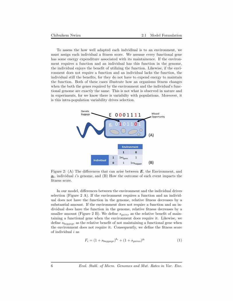
To assess the how well adapted each indvidiual is to an environment, wemust assign each individual a fitness score. We assume every functional genehas some energy expenditure associated with its maintainence. If the environ-ment requires a function and an individual has this function in the genome,the individual enjoys the benefit of utilizing the function. Likewise, if the envi-ronment does not require a function and an individual lacks the function, theindividual still the benefits, for they do not have to expend energy to maintainthe function. Both of these cases illustrate how an organisms fitness changeswhen the both the genes required by the environment and the individual’s func-tional genome are exactly the same. This is not what is observed in nature andin experiments, for we know there is variabilty with populations. Moreover, itis this intra-population variability drives selection.

Figure 2: (A) The differences that can arise between E, the Environment, andgi, individual i ’s genome, and (B) How the outcome of each event impacts thefitness score.

In our model, differences between the environment and the individual drivesselection (Figure 2 A). If the environment requires a function and an individ-ual does not have the function in the genome, relative fitness decreases by asubstantial amount. If the environment does not require a function and an in-dividual does have the function in the genome, relative fitness decreases by asmaller amount (Figure 2 B). We define sgains as the relative benefit of main-taining a functional gene when the environment does require it. Likewise, wedefine sbaggage as the relative benefit of not maintaining a functional gene whenthe environment does not require it. Consequently, we define the fitness scoreof individual i as

Fi = (1 + sbaggage)bi + (1 + sgains)

gi (1)


Chibuikem Nwizu 2.1 Model Formulation

wherebi =

∑j

1b(xij , ej)

gi =∑j

1g(xij , ej)(2)

and 1b and 1g are indicator functions that are 1 when xij = ej = 0 (in the caseof 1b) or xij = ej = 1 (in the case of 1g), but are zero otherwise.

We employ a Wright-Fischer Model for selection to model selection in ourpopulation. In Wright-Fischer, individuals are stochastically choosen to re-produce in proportion to their fitness in the current environment— the valuerepresented in equation 1. Using Wright-Fisher, the allelic composition of thepopulation changes, but the total population size remains fixed at N. We willnot discuss how Wright-Fisher selection works in this paper, only mention itsuse. Again, by employing Wright-Fisher, we encorperate the obsereved stochas-ticity of selection into our model: Though an organism may have a high fitnessscore, it does not gaurentee their survival in an environment, only increasestheir probability of surviving.

We also include mutations in our model. Mutations in nature occur as anerror in the copying of genetic information from parent to offspring– manifestingitself from small events like single nucleotide substitution, to large large eventslike a chromosome insertion/deletion. As previously noted, mutations are amajor driver for genetic variability within a population. Likewise, within ourmodel, mutations drive intra-population variability.

We define µ as the per loci per individual knockout mutation rate (that isthe rate of 1 → 0). In the accessory genome, we model the number of knockoutmutations as a Binomial random variable

XKO ∼ Bino(nfunc, µ) (3)

where nfunc is the total number of functional sites available in accessory genomesaccross the population.

Likewise, we define µr as the per loci per individual reverse mutation rate(that is 0 → 1) occur per loci per individual. We assume that the reversemutations rate are proportional to knockout mutation rate

µr = r ∗ µ, r ∈ [0, 1)

We model the number of reverse mutations also as a Binomial random vari-able

XRev ∼ Bino(nnon−func, µr) (4)

where nnon−func is the total number of non-functional sites available in acces-sory genomes accross the population.

Mutations can occur in our core genome (though it is not explicitly mod-elled). We also assume that a mutation to the core genome is automaticallylethal. We model the number of lethal mutations as a Poisson random variable

XLeth ∼ Poi(λ) (5)


Chibuikem Nwizu 2.2 The Simple Model

where λ = nessential ∗ µ, and represents the average number of times mutationoccurs in the core genome (nessential).

Our next parameter is the fraction needed. We define fraction needed (f) asthe probability that any particular gene at loci j will be required by any partic-ular enviroment. Such a parameter is important because it is unknown exactlyhow much of the accessory genome is needed by any particular environment.However, our model is sensitive to this: if the environment, E, requires a highnumber of ones, selection will favor inviduals who maintain a higher numberof ones. Addtionally, If the environment changes, we would want the aver-age number of genes required to remain constant across environmental changes.This allows us to observe how requiring different functions effects the long termgenome diversity and complexity of the accessory genome.

Related to f is the rate at which the environment changes. We define τ asthe wait time between environmental changes (the change rate is technically 1

τbut we will refer to τ as the change rate). When τ is small, the environmentchanges very quickly, and when τ is large, the environment changes very slowly.

2.2 The Simple Model

To build intuition, we start by examining the behavior of the model with onlyn = 1 locus.

2.2.1 Equilbrium dynamics of 1 Loci

We looked at the fraction of ones at equilibrium for very small τ . We define thefraction of 1’s in the population as

pj =

∑i xijN

(6)

With this definition, we were able to write a deterministic description for therate of the fraction of ones at locus j=1.

dpjdt

=− µ pj + µr(1− pj)

− f sgains pj − (1− f) sbaggage pj

+ (1− f) sbaggage (1− pj) + f sgains (1− pj)

(7)

This deterministic treatment of the model assumes that the environment changesrapidly. For very small tau, the environment changes so quickly that any oneindividual experiences many enviroments. Consequently, the behaviour of the1-loci model for small tau at equilibrium can be modelled with the fraction ofones at equilibrium

p∞ =f sgains − (1− f) sbaggage + µr

µ+ µr + f sgains(8)


Chibuikem Nwizu

3 Results

3.1 Non-Equilibrium Behavior

First, we would like to understand the pre-equilibrium behaviour of the model.Understanding this behavior will provide intuition about the forces that impactour model and insight into the qualitative tendenicies of the a population’s ac-cessory genome. In particular, we would like to understand the pre-equilibriumdynamics of the functional genes in a population’s accessory genome. Becausethe most mutations are loss of function mutations, we expect the number offunctional genes to decay with time. As the functional genes decays, the popu-lation becomes more specialized, able to tolerate less unique environments thatrequire unique mutations. Consequently, we will call this metric the rate ofspecialization, S∗. We define the average rate of specialization, S∗, over allreplicates as

S∗ =1

r

r∑max

{dp∗rdt

}where p∗ is the fraction of functional genes accross the entire population for asingle replicate, and r is the number of replicates.

There will be certain parameter regimes that increase S∗. Regimes thatpromote faster specialization will favor accessory genomes that are closer to thefunctional genes required by the environment. These genomes have a selectiveadvantage and will sweep the population, lowering the fraction of functionalgenes in the population. We define these genomes as specialist genomes (spe-icalists). Specialists have the functional genes required by the current envi-ronment therefore they experience a selective advantage in these regimes. Onthe other hand, we define generalist genomes (generalists) as genomes that spe-cialize slower, but are more aptly suited for surviving many different types ofenvironments.


Chibuikem Nwizu 3.1 Non-Equilibrium Behavior

Figure 3: Large values of τ mark a regime where specialists are favored. Thesimulation parameters were sgains = 0.1, sbaggage = 0.01, f = 0.2, µ1 = 10−5.

When we increased τ , S∗ increased. Figure 3 shows this trend. For smallτs, generalists are favored because their high functional gene content allowsthem to be better suited for a wider variety of environments. This drives thepopulation’s fraction functional genes up. Large τs favor specialists because,during the simulation time, their genomes converge faster to the functional genesrequired by the environment. This provides them with a selective advantage andallows them to sweep the population.

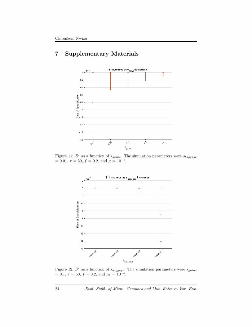
When we increased sgains, S∗ decreased (see Figure 11 in Supplemental Ma-terials). Thinking about the model, we are able to gain intuition about thisresult. As the population evolves, individuals with too many loss of functionmutations are selected against. Consequently, increasing sgains selects for indi-vidual who maintain lots of functional genes in their genome. As the generalistssurvive and increase in frequency, their genomes prevent the decay of functionalgenes in the population, slowing the rate of specialization.

When we increased sbaggage, S∗ increased (see Figure 12 in SupplementalMaterials). In our model, sbaggage is given when the individual loses a func-tional gene, and the environment does not require it. Specialists are more likelyto have lots of zeros that match the environment; therefore, sbaggage favors thespecialists. Since specialists are favored and they tend to carry fewer func-tional genes, the fraction of functional genes in the population is driven down,increasing S∗.

When we increased f , S∗ increased (see Figure 13 in Supplemental Materi-als). f is the fraction of time loci i is needed. A larger f corresponds to moregenes being required in every environment. Consequently, the generalist is fa-vored over the specialist for their genomes contain more functional genes. This


Chibuikem Nwizu 3.2 Equilibrium Behavior

maintains a high fraction of functional genes in the population, slowing the rateof specialization.

Finally, when we increased µ1, S∗ decreased (see Figure 14 in Supplemen-tal Materials). As µ1 increases, more loss of function mutations occur. Thispromotes the creation of specialists. With more specialists, the fraction of func-tional genes in the population is driven down, increasing S∗.

Table 1 below summarizes the results of the results of the simulations

Table 1: Summary of the effects of the model parameters on S∗

Change Effect on S∗

τ ↑ ↑sgains ↑ ↓sbaggage ↑ ↑f ↑ ↓µ2 ↑ ↑

3.2 Equilibrium Behavior

3.2.1 Equilibrium Behavior of Genome Complexity

Figure 4: Genome Complexity at equilibrium is stablized by fast-changing en-vironments.

We looked at the number of functional genes at equilibrium to understand theeffect of variable environments on pan-genomic complexity. Figure 4 showsthe fraction of functional genes at equilibrium, Feq. For large τ values, Feq



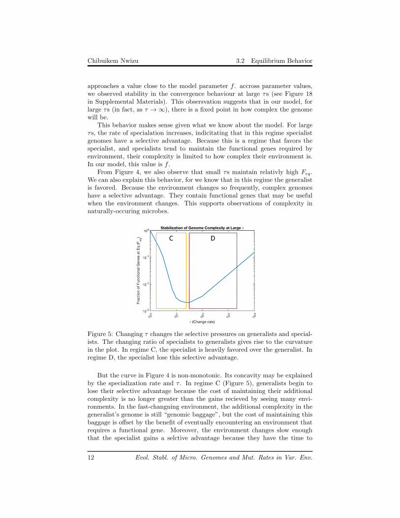
approaches a value close to the model parameter f . accross parameter values,we observed stability in the convergence behaviour at large τs (see Figure 18in Supplemental Materials). This obsersvation suggests that in our model, forlarge τs (in fact, as τ →∞), there is a fixed point in how complex the genomewill be.

This behavior makes sense given what we know about the model. For largeτs, the rate of specialation increases, indicitating that in this regime specialistgenomes have a selective advantage. Because this is a regime that favors thespecialist, and specialists tend to maintain the functional genes required byenvironment, their complexity is limited to how complex their environment is.In our model, this value is f .

From Figure 4, we also observe that small τs maintain relativly high Feq.We can also explain this behavior, for we know that in this regime the generalistis favored. Because the environment changes so frequently, complex genomeshave a selective advantage. They contain functional genes that may be usefulwhen the environment changes. This supports observations of complexity innaturally-occuring microbes.

Figure 5: Changing τ changes the selective pressures on generalists and special-ists. The changing ratio of specialists to generalists gives rise to the curvaturein the plot. In regime C, the specialist is heavily favored over the generalist. Inregime D, the specialist lose this selective advantage.

But the curve in Figure 4 is non-monotonic. Its concavity may be explainedby the specialization rate and τ . In regime C (Figure 5), generalists begin tolose their selective advantage because the cost of maintaining their additionalcomplexity is no longer greater than the gains recieved by seeing many envi-ronments. In the fast-changning environment, the additional complexity in thegeneralist’s genome is still “genomic baggage”, but the cost of maintaining thisbaggage is offset by the benefit of eventually encountering an environment thatrequires a functional gene. Moreover, the environment changes slow enoughthat the specialist gains a selctive advantage because they have the time to



specialize.In regime D (Figure 5), this advantage diminishes, resulting in the upward

inflection of the curve. The specialists continue to have a selective advantageduring moderate τs; however, these extended periods in a particular environ-ment causes them to overspecialize on that particular environment. When theenvironment changes, it is likely they have lost the genes needed for the newenvironment. Therefore, moderate specialists with enough complexity (in fact,with the complexity closest to f) are selected for, raising the value of Feq to f .

3.2.2 Equilibrium Behavior of Genome Diversity

Figure 6: Pan-genome diversity at equilibrium is maximized in moderately-changing environments.

Next, we looked the Shannon Index of the population at equilibrium to un-derstand the effect of varying environments on the pan-genomic diversity. Toquantify diversity, we used the Shannon Index:

H ′ =∑i

hi lnhi

where hi is the fraction of individuals with genome i. Figure 6 shows the AverageShannon Index, H ′, at equilibrium. The behavior of the plot at extremelylarge and extremely small values of τ show that diversity is very low at bothextremes. This suggests that only only one type group exists at both extremes:specialists, when τ is large, and generalists, when τ is small. Moreover, for largeτs, H ′ appears to converge to the same value for the same f , across independentsimulation runs.



Based on our understanding of the model, the diversity behavior of pan-genomes at equilibrium appears to converge due to the dominance of specialistsin this regime. We can explain why converges through the S∗ and Feq. We knowit is converging because constant environments favor genomic convergence to f(Figure 3). Furthermore, we know they are converging to the same complexityvalue (Figure 4). Diversity shrinks because selection favors the specialist andforces genomes to converge to the environments complexity.

From Figure 6, we see that small τs also promote convergence. In thisregime, the generalist dominate. Since, diversity is low we know that there areonly a few unique genomes; however, only a few unique generalist genomes areneeded to maintain the complexity observed in Figure 4. These genomes havethe raw genomic material to cause a diversity explosion. Selection, however,prevents this. For large enough subpopulations, selection can not make a gen-eralist lineage more diverse. The diversification only occurs through mutation.However, for low mutation rates, after generalist lineages split into a parent andchild branch, the child branch is small in size and subject to drift. Therefore,selection keeps diversity low in rapidly changing environments.

Figure 7: Behavior in intermediate regions are explained by S∗ and Feq.

In regime C (Figure 7), the diversity increases. This increase may be dueto two factors that work in concert: (1) there are generalists to provide thegenetic raw material for diversity and (2) selection begins to favor specialistsmore, allowing smaller lineages to grow and extablish.

Likewise, the decrease in diversity in regime D (Figure 7), could be due to thelack of generalist: Specialization increases during this time and and degradesthe genomic diversity. Another factor that could contribute to the decline isthat in this regime, selection for specialists decreases. The true explanation islikely a combination of the both of the aforementioned hypotheses.


Chibuikem Nwizu 3.3 The Fate of a Mutator in variable Environments

3.3 The Fate of a Mutator in variable Environments

We have defined the specialist by the content of their genome. In this section,we will expand the definition to include all types of genomes with an elevatedmutation rate. These types of specialists are called mutators.

It is important to expand the definition of specialists to include mutatorsbecause much of the constant environment behavior noted in this report hasbeen exhibited in mutators in controlled evolution experiments under labora-tory conditions [33, 40]. Namely, many studies have observed that laboratorypopulations of prokaryotes evolve higher mutation rates. Unlike there labora-tory counterparts, natural populations tend to evolve lower mutation rates [32].We seek to understand how varying environments stablize mutation rate us-ing our model. Moreover, we would like to understand the fate of mutators invariable envirnoments.

We are able to expand the definition of a specialist because most mutationsbreak genes. We have seen that non-functional genes create a selection differ-ence. We have observed that it is this difference in selection that changes thetrajectory of the allelic composition of the population. With the present modelwe seek to understand the fate of mutators in variable environments, and theeffect that the model parameters have on the mutator’s fate.

Figure 8: Mutators are have a selective advantage in slow-changing environ-ments. The simulation parameters were sgains = 0.1, sbaggage = 0.01, f = 0.2,and µ2 = 10−5.

As τ increased, the mutator’s fixation probability increased. Figure 8 showsthis trend. The dashed line is at 1

N and indicates the point at which the τgoes from deleterious to beneficial. The results of this simulation indicate a



very defined point of neutrality exists for that particular set of parameters. Thepoint of neutrality appears to be between τ = 50 and τ = 75. As τ increases, theenvironment changes at a slower rate, meaning the mutator is allowed more timeto specialize on a particular environment. This explaination is corroborated byexperimental observation [33, 40].

The impact of the other parameters in noted in Table 2 below. When we in-creased sgains, the fixation probability decreased (see Figure 15 in SupplementalMaterials). Thinking about the model, we gain intuition about this result, mu-tators tend to lose functional mutations faster than the wildtype. In an changingenvironment, they may begin to lose functional genes not needed in one envi-ronment quickly, but when the environment changes and they encounter a newenvironment that may require this function, they are at a disadvantage exactlylike a specialist would in the same scenerio. As the cost of this disadvantagegrows, the mutator selected against.

As we increased sbaggage, the fixation probability decreased (see Figure 16 inSupplemental Materials). The results of this simulation is more pronounced, andthe effects of sbaggage appears to have a large impact on Pfix. To gain intuitionabout this results, we note that when loosing functions is very beneficial, themutator will be favored for they tend to loose functional mutations faster thanthe wildtype. The results suggest that this benefit is strong enough to dominateeven as the environment changes.

When f increases, fixation probability increased (see Figure 17 in Supple-mental Materials in Supplementals). Because f is the fraction of time, loci iis needed, larger f mean that more genes are required in every environment.In these cases, the mutator disadvantaged because their tendency to lose func-tional genes means they are not able to maintain the fraction of ones need inany particular environment.



Figure 9: In fluctating environments (τ = 100), mutation rate appears to stablesat moderate values. The simulation parameters were sgains = 0.1, sbaggage =0.01, and f = 0.2.

Finally, as µ2 increases, Pfix behaves non-monotonic. Figure 9 shows thistrend. The result suggest there is a non-monotonic relationship between µ2 andPfix. For extreme values of µ2, Pfix appears to be small. This suggest for thisparticular parameter set, there is an optimum mutation rate. Unlike any ofthe parameters, µ2 appears to be deleterious for extreme values of µ2; howeverfor median values of µ2 appear to be beneficial. The threshold is between1× 10−6 < µ2 < 5× 10−6 and 5× 10−5 < µ2 < 5× 10−4. The presences of twothreshold suggests that µ2 is stablized in variable environments. This could bebcause when µ2 is smaller than the wildtype’s mutation rate, µ1, it is unable tobreak genes as well as the wildtype and must pay the cost of carrying aroundgenetic baggage. But when µ2 is much larger than the µ1, it will specilize tooquickly on the environment, and pay the cost of not having the right functionwhen the environment changes. Additionally, when µ2 is much larger than theµ1, it also overspecializes on the current environment, and break essential genes.Table 2 below summarizes the results of the results of the simulations

Table 2: Summary of the effects of the model parameters on Pfix

Change Effect on Pfixτ ↑ ↑sgains ↑ ↓sbaggage ↑ ↑f n ↑ ↓µ2 ↑ l


Chibuikem Nwizu

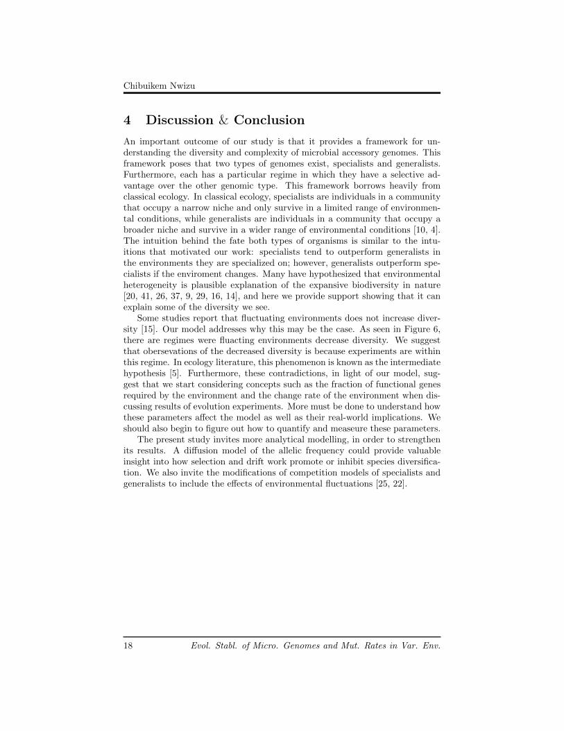
4 Discussion & Conclusion

An important outcome of our study is that it provides a framework for un-derstanding the diversity and complexity of microbial accessory genomes. Thisframework poses that two types of genomes exist, specialists and generalists.Furthermore, each has a particular regime in which they have a selective ad-vantage over the other genomic type. This framework borrows heavily fromclassical ecology. In classical ecology, specialists are individuals in a communitythat occupy a narrow niche and only survive in a limited range of environmen-tal conditions, while generalists are individuals in a community that occupy abroader niche and survive in a wider range of environmental conditions [10, 4].The intuition behind the fate both types of organisms is similar to the intu-itions that motivated our work: specialists tend to outperform generalists inthe environments they are specialized on; however, generalists outperform spe-cialists if the enviroment changes. Many have hypothesized that environmentalheterogeneity is plausible explanation of the expansive biodiversity in nature[20, 41, 26, 37, 9, 29, 16, 14], and here we provide support showing that it canexplain some of the diversity we see.

Some studies report that fluctuating environments does not increase diver-sity [15]. Our model addresses why this may be the case. As seen in Figure 6,there are regimes were fluacting environments decrease diversity. We suggestthat obersevations of the decreased diversity is because experiments are withinthis regime. In ecology literature, this phenomenon is known as the intermediatehypothesis [5]. Furthermore, these contradictions, in light of our model, sug-gest that we start considering concepts such as the fraction of functional genesrequired by the environment and the change rate of the environment when dis-cussing results of evolution experiments. More must be done to understand howthese parameters affect the model as well as their real-world implications. Weshould also begin to figure out how to quantify and measeure these parameters.

The present study invites more analytical modelling, in order to strengthenits results. A diffusion model of the allelic frequency could provide valuableinsight into how selection and drift work promote or inhibit species diversifica-tion. We also invite the modifications of competition models of specialists andgeneralists to include the effects of environmental fluctuations [25, 22].


Chibuikem Nwizu

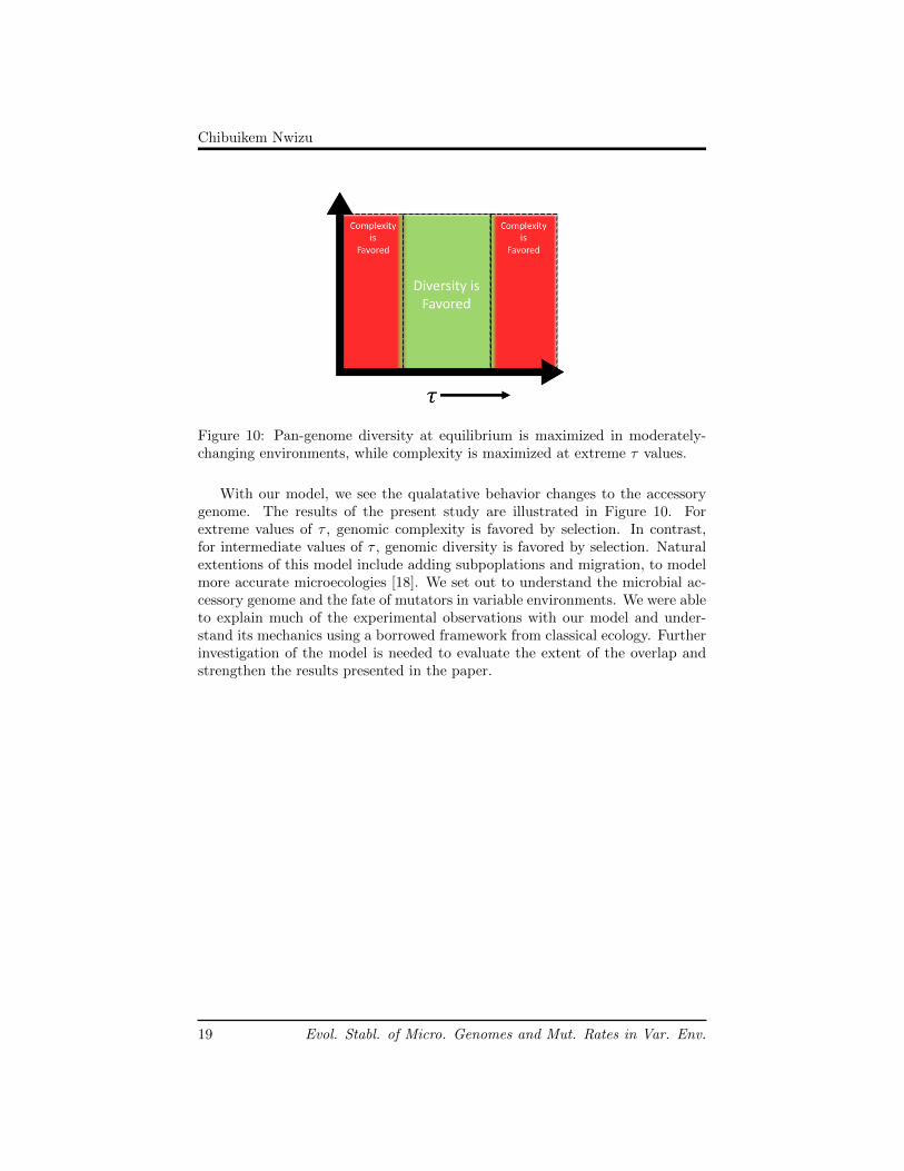
Figure 10: Pan-genome diversity at equilibrium is maximized in moderately-changing environments, while complexity is maximized at extreme τ values.

With our model, we see the qualatative behavior changes to the accessorygenome. The results of the present study are illustrated in Figure 10. Forextreme values of τ , genomic complexity is favored by selection. In contrast,for intermediate values of τ , genomic diversity is favored by selection. Naturalextentions of this model include adding subpoplations and migration, to modelmore accurate microecologies [18]. We set out to understand the microbial ac-cessory genome and the fate of mutators in variable environments. We were ableto explain much of the experimental observations with our model and under-stand its mechanics using a borrowed framework from classical ecology. Furtherinvestigation of the model is needed to evaluate the extent of the overlap andstrengthen the results presented in the paper.


Chibuikem Nwizu

5 Methods

We ran simulations using a combination of R2014a, Matlab 2015a, 2015b, and2016a. Jobs were run on the Brown University CCV or on local machines. Thegenome of the organism was represented a by a one-dimensional array of 1’s and0’s where each index corresponds to a locus on the genome. A 1 correspondsto function at that particular locus. A 0 corresponds to no function at thatparticular locus. Each locus is independent of one another. The population wasfed into a mutation function that, based on the mutation rate, performed loss offunction mutations, gain of function mutations, and lethal mutations. A loss offunction mutation refers to the conversion of a 1 to a 0 on the nonessential lociof the genome. A gain of function mutation refers to the conversion of a 0 toa 1 nonessential loci of the genome. A lethal mutation refers to the conversionof a 1 to a 0 on essential loci of the genome. A matrix of all of the individualbit string constituted a population. The environment was also represented aby a one-dimensional array of 1’s and 0’s where each index corresponds to alocus on the genome. Then environment frequently based on the parameter τ .We calculated the fitness of each organism in a population at a particular timestep. To calculate the fitness, each row in the population matrix was comparedto the environmental array. If the value at locus i agreed with the environmentat locus, and the value was 1, the organism’s fitness score is added to by a theamount 1 + sgain. If the value at locus i agreed with the environment at locus,and the value was 0, the organism’s fitness score is added to by a the amount1 + sbaggage. The fitness score were feed into a Wright-Fisher function, thatselected the individuals reproduce based on the fitness values. Termination ofthe simulation was dependent on the type of simulation: fixation simulation wereterminated when either the mutant fixed or went extinct; all other simulationsterminated after a defined number of generations.

6 Acknowledgements

I would like to thank my mentor and friend Christopher Graves for the work hehas done in advising, guiding, and mentoring me through this research journey.Without Chris, I would not have been able to complete this project. I wouldalso like to acknowledge the Weinreich lab (both its Principle Investigator, Dr.Daniel Weinreich, and its current/former memebers) for giving me a researchhome these past two years. I am very appriciative of the opportunities and ex-periences given to me, for the have allowed me to mature and grow intellectualy.

References

[1] D. Berger, R. J. Walters, and W. U. Blanckenhorn, Experimentalevolution for generalists and specialists reveals multivariate genetic con-straints on thermal reaction norms, Journal of Evolutionary Biology, 27(2014), pp. 1975–1989.


Chibuikem Nwizu REFERENCES

[2] S. Casjens, The diverse and dynamic structure of bacterial genomes, An-nual review of genetics, 32 (1998), pp. 339–377.

[3] S. Casjens, N. Palmer, R. Van Vugt, W. Mun Huang, B. Steven-son, P. Rosa, R. Lathigra, G. Sutton, J. Peterson, R. J. Dodson,et al., A bacterial genome in flux: the twelve linear and nine circular ex-trachromosomal dnas in an infectious isolate of the lyme disease spirocheteborrelia burgdorferi, Molecular microbiology, 35 (2000), pp. 490–516.

[4] A. Colles, L. H. Liow, and A. Prinzing, Are specialists at risk un-der environmental change? neoecological, paleoecological and phylogeneticapproaches, Ecology Letters, 12 (2009), pp. 849–863.

[5] J. H. Connell, Diversity in tropical rain forests and coral reefs, Science,199 (1978), pp. 1302–1310.

[6] U. Dobrindt and J. Hacker, Whole genome plasticity in pathogenicbacteria, Current opinion in microbiology, 4 (2001), pp. 550–557.

[7] C. Dutta and A. Pan, Horizontal gene transfer and bacterial diversity,Journal of biosciences, 27 (2002), pp. 27–33.

[8] L. S. Frost, R. Leplae, A. O. Summers, and A. Toussaint, Mo-bile genetic elements: the agents of open source evolution, Nature ReviewsMicrobiology, 3 (2005), pp. 722–732.

[9] D. J. Futuyma and G. Moreno, The evolution of ecological specializa-tion, Annual Review of Ecology and Systematics, 19 (1988), pp. 207–233.

[10] G. W. Gilchrist, Specialists and generalists in changing environments.i. fitness landscapes of thermal sensitivity, The American Naturalist, 146(1995), pp. 252–270.

[11] A. Giraud, I. Matic, O. Tenaillon, A. Clara, M. Radman,M. Fons, and F. Taddei, Costs and benefits of high mutation rates: adap-tive evolution of bacteria in the mouse gut, Science, 291 (2001), pp. 2606–2608.

[12] L. R. Hallsson and M. Bjorklund, Selection in a fluctuating environ-ment leads to decreased genetic variation and facilitates the evolution ofphenotypic plasticity, Journal of evolutionary biology, 25 (2012), pp. 1275–1290.

[13] A. K. Hottes, P. L. Freddolino, A. Khare, Z. N. Donnell, J. C.Liu, and S. Tavazoie, Bacterial adaptation through loss of function, PLoSGenet, 9 (2013), p. e1003617.

[14] Y. Huang, J. R. Stinchcombe, and A. F. Agrawal, Quantitativegenetic variance in experimental fly populations evolving with or withoutenvironmental heterogeneity, Evolution, 69 (2015), pp. 2735–2746.



[15] S. M. Karve, K. Tiwary, S. Selveshwari, and S. Dey, Environmen-tal fluctuations do not select for increased variation or population-basedresistance in escherichia coli, Journal of biosciences, 41 (2016), pp. 39–49.

[16] R. Kassen, The experimental evolution of specialists, generalists, andthe maintenance of diversity, Journal of evolutionary biology, 15 (2002),pp. 173–190.

[17] D. J. Kvitek and G. Sherlock, Whole genome, whole population se-quencing reveals that loss of signaling networks is the major adaptive strat-egy in a constant environment, PLoS Genet, 9 (2013), p. e1003972.

[18] N. Lanchier and C. Neuhauser, A spatially explicit model for competi-tion among specialists and generalists in a heterogeneous environment, TheAnnals of Applied Probability, (2006), pp. 1385–1410.

[19] P. Lapierre and J. P. Gogarten, Estimating the size of the bacterialpan-genome, Trends in genetics, 25 (2009), pp. 107–110.

[20] R. C. Lewontin et al., The genetic basis of evolutionary change,vol. 560, Columbia University Press New York, 1974.

[21] D. Medini, C. Donati, H. Tettelin, V. Masignani, and R. Rap-puoli, The microbial pan-genome, Current opinion in genetics & develop-ment, 15 (2005), pp. 589–594.

[22] A. Melbinger and M. Vergassola, The impact of environmental fluc-tuations on evolutionary fitness functions, arXiv preprint arXiv:1510.05664,(2015).

[23] A. Mira, L. Klasson, and S. G. Andersson, Microbial genome evo-lution: sources of variability, Current opinion in microbiology, 5 (2002),pp. 506–512.

[24] A. Mira, H. Ochman, and N. A. Moran, Deletional bias and the evo-lution of bacterial genomes, Trends in Genetics, 17 (2001), pp. 589–596.

[25] C. Neuhauser and S. W. Pacala, An explicitly spatial version of thelotka-volterra model with interspecific competition, Annals of Applied Prob-ability, (1999), pp. 1226–1259.

[26] E. Nevo, Genetic variation in natural populations: patterns and theory,Theoretical population biology, 13 (1978), pp. 121–177.

[27] V. C. Nwosu, Antibiotic resistance with particular reference to soil mi-croorganisms, Research in Microbiology, 152 (2001), pp. 421–430.

[28] H. Ochman, J. G. Lawrence, and E. A. Groisman, Lateral genetransfer and the nature of bacterial innovation, Nature, 405 (2000), pp. 299–304.



[29] M. L. Rosenzweig, Species diversity in space and time, Cambridge Uni-versity Press, 1995.

[30] L. Rouli, V. Merhej, P.-E. Fournier, and D. Raoult, The bacterialpangenome as a new tool for analysing pathogenic bacteria, New microbesand new infections, 7 (2015), pp. 72–85.

[31] P. D. Sniegowski, P. J. Gerrish, T. Johnson, A. Shaver, et al.,The evolution of mutation rates: separating causes from consequences,Bioessays, 22 (2000), pp. 1057–1066.

[32] P. D. Sniegowski, P. J. Gerrish, and R. E. Lenski, Evolution of highmutation rates in experimental populations of e. coli, Nature, 387 (1997),p. 703.

[33] M. M. Tanaka, C. T. Bergstrom, and B. R. Levin, The evolution ofmutator genes in bacterial populations: the roles of environmental changeand timing, Genetics, 164 (2003), pp. 843–854.

[34] H. Tettelin, D. Riley, C. Cattuto, and D. Medini, Comparativegenomics: the bacterial pan-genome, Current opinion in microbiology, 11(2008), pp. 472–477.

[35] C. M. Thomas and K. M. Nielsen, Mechanisms of, and barriers to,horizontal gene transfer between bacteria, Nature reviews microbiology, 3(2005), pp. 711–721.

[36] E. R. Tillier and R. A. Collins, Genome rearrangement by replication-directed translocation, Nature genetics, 26 (2000), pp. 195–197.

[37] D. Tilman, Resource competition and community structure, Princeton uni-versity press, 1982.

[38] V. Torsvik, L. Øvreas, and T. F. Thingstad, Prokaryotic diversity–magnitude, dynamics, and controlling factors, Science, 296 (2002),pp. 1064–1066.

[39] M. Touchon and E. P. Rocha, Causes of insertion sequences abun-dance in prokaryotic genomes, Molecular biology and evolution, 24 (2007),pp. 969–981.

[40] J. Travis and E. Travis, Mutator dynamics in fluctuating environments,Proceedings of the Royal Society of London B: Biological Sciences, 269(2002), pp. 591–597.

[41] R. H. Whittaker and S. A. Levin, Niche: theory and application,Dowden, Hutchinson & Ross Stroudsbourg, 1975.


Chibuikem Nwizu

7 Supplementary Materials

Figure 11: S∗ as a function of sgains. The simulation parameters were sbaggage= 0.01, τ = 50, f = 0.2, and µ = 10−5.

Figure 12: S∗ as a function of sbaggage. The simulation parameters were sgains= 0.1, τ = 50, f = 0.2, and µ1 = 10−5.


Chibuikem Nwizu

Figure 13: S∗ as a function of f . The simulation parameters were sgains =0.1,sbaggage = 0.01, τ = 50, and µ1 = 10−5.

Figure 14: S∗ as a function of µ. The simulation parameters were sgains = 0.1,sbaggage = 0.01, τ = 50, and f = 0.2.


Chibuikem Nwizu

Figure 15: Pfix decreases as a function of sgains. The simulation parameterswere sbaggage = 0.01, τ = 50, f = 0.2, and µ2 = 10−5.

Figure 16: Pfix increases as a function of sbaggage. The simulation parameterswere sgains = 0.1, τ = 50, f = 0.2, and µ2 = 10−5


Chibuikem Nwizu

Figure 17: Pfix decreases as a function of f . The simulation parameters weresgains = 0.1, sbaggage = 0.01, τ = 50, and µ2 = 10−5.

Figure 18: Genome Complexity for large τ converge to the f = 0.20


evolutionary stabilization of microbial genomes and ... · department of applied mathematics, ......

Documents