evolving artiﬁcial neural networksxin/papers/published_iproc_sep99.pdf · evolving artiﬁcial...

Evolving Artificial Neural Networks

XIN YAO, SENIOR MEMBER, IEEE

Invited Paper

Learning and evolution are two fundamental forms of adapta-tion. There has been a great interest in combining learning andevolution with artificial neural networks (ANN’s) in recent years.This paper: 1) reviews different combinations between ANN’s andevolutionary algorithms (EA’s), including using EA’s to evolveANN connection weights, architectures, learning rules, and inputfeatures; 2) discusses different search operators which have beenused in various EA’s; and 3) points out possible future researchdirections. It is shown, through a considerably large literaturereview, that combinations between ANN’s and EA’s can lead tosignificantly better intelligent systems than relying on ANN’s orEA’s alone.

Keywords—Evolutionary computation, intelligent systems, neu-ral networks.

I. INTRODUCTION

Evolutionary artificial neural networks (EANN’s) referto a special class of artificial neural networks (ANN’s) inwhich evolution is another fundamental form of adaptationin addition to learning [1]–[5]. Evolutionary algorithms(EA’s) are used to perform various tasks, such as con-nection weight training, architecture design, learning ruleadaptation, input feature selection, connection weight ini-tialization, rule extraction from ANN’s, etc. One distinctfeature of EANN’s is their adaptability to a dynamicenvironment. In other words, EANN’s can adapt to an en-vironment as well as changes in the environment. The twoforms of adaptation, i.e., evolution and learning in EANN’s,make their adaptation to a dynamic environment much moreeffective and efficient. In a broader sense, EANN’s can beregarded as a general framework for adaptive systems, i.e.,systems that can change their architectures and learningrules appropriately without human intervention.

This paper is most concerned with exploring possiblebenefits arising from combinations between ANN’s andEA’s. Emphasis is placed on the design of intelligentsystems based on ANN’s and EA’s. Other combinations

Manuscript received July 10, 1998; revised February 18, 1999. Thiswork was supported in part by the Australian Research Council throughits small grant scheme.

The author is with the School of Computer Science, Universityof Birmingham, Edgbaston, Birmingham B15 2TT U.K. (e-mail:[email protected]).

Publisher Item Identifier S 0018-9219(99)06906-6.

between ANN’s and EA’s for combinatorial optimizationwill be mentioned but not discussed in detail.

A. Artificial Neural Networks

1) Architectures: An ANN consists of a set of processingelements, also known as neurons or nodes, which areinterconnected. It can be described as a directed graph inwhich each node performs a transfer function of theform

(1)

where is the output of the node is the th input tothe node, and is the connection weight between nodes

and . is the threshold (or bias) of the node. Usually,is nonlinear, such as a heaviside, sigmoid, or Gaussian

function.ANN’s can be divided into feedforward and recurrent

classes according to their connectivity. An ANN is feed-forward if there exists a method which numbers all thenodes in the network such that there is no connection froma node with a large number to a node with a smaller number.All the connections are from nodes with small numbers tonodes with larger numbers. An ANN is recurrent if such anumbering method does not exist.

In (1), each term in the summation only involves oneinput . High-order ANN’s are those that contain high-order nodes, i.e., nodes in which more than one inputare involved in some of the terms of the summation. Forexample, a second-order node can be described as

where all the symbols have similar definitions to those in(1).

The architecture of an ANN is determined by its topo-logical structure, i.e., the overall connectivity and transferfunction of each node in the network.

0018–9219/99$10.00 1999 IEEE

PROCEEDINGS OF THE IEEE, VOL. 87, NO. 9, SEPTEMBER 1999 1423

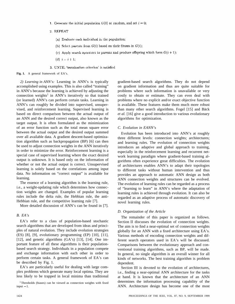
Fig. 1. A general framework of EA’s.

2) Learning in ANN’s: Learning in ANN’s is typicallyaccomplished using examples. This is also called “training”in ANN’s because the learning is achieved by adjusting theconnection weights1 in ANN’s iteratively so that trained(or learned) ANN’s can perform certain tasks. Learning inANN’s can roughly be divided into supervised, unsuper-vised, and reinforcement learning. Supervised learning isbased on direct comparison between the actual output ofan ANN and the desired correct output, also known as thetarget output. It is often formulated as the minimizationof an error function such as the total mean square errorbetween the actual output and the desired output summedover all available data. A gradient descent-based optimiza-tion algorithm such as backpropagation (BP) [6] can thenbe used to adjust connection weights in the ANN iterativelyin order to minimize the error. Reinforcement learning is aspecial case of supervised learning where the exact desiredoutput is unknown. It is based only on the information ofwhether or not the actual output is correct. Unsupervisedlearning is solely based on the correlations among inputdata. No information on “correct output” is available forlearning.

The essence of a learning algorithm is the learning rule,i.e., a weight-updating rule which determines how connec-tion weights are changed. Examples of popular learningrules include the delta rule, the Hebbian rule, the anti-Hebbian rule, and the competitive learning rule [7].

More detailed discussion of ANN’s can be found in [7].

B. EA’s

EA’s refer to a class of population-based stochasticsearch algorithms that are developed from ideas and princi-ples of natural evolution. They include evolution strategies(ES) [8], [9], evolutionary programming (EP) [10], [11],[12], and genetic algorithms (GA’s) [13], [14]. One im-portant feature of all these algorithms is their population-based search strategy. Individuals in a population competeand exchange information with each other in order toperform certain tasks. A general framework of EA’s canbe described by Fig. 1.

EA’s are particularly useful for dealing with large com-plex problems which generate many local optima. They areless likely to be trapped in local minima than traditional

1Thresholds (biases) can be viewed as connection weights with fixedinput�1.

gradient-based search algorithms. They do not dependon gradient information and thus are quite suitable forproblems where such information is unavailable or verycostly to obtain or estimate. They can even deal withproblems where no explicit and/or exact objective functionis available. These features make them much more robustthan many other search algorithms. Fogel [15] and Backet al. [16] give a good introduction to various evolutionaryalgorithms for optimization.

C. Evolution in EANN’s

Evolution has been introduced into ANN’s at roughlythree different levels: connection weights; architectures;and learning rules. The evolution of connection weightsintroduces an adaptive and global approach to training,especially in the reinforcement learning and recurrent net-work learning paradigm where gradient-based training al-gorithms often experience great difficulties. The evolutionof architectures enables ANN’s to adapt their topologiesto different tasks without human intervention and thusprovides an approach to automatic ANN design as bothANN connection weights and structures can be evolved.The evolution of learning rules can be regarded as a processof “learning to learn” in ANN’s where the adaptation oflearning rules is achieved through evolution. It can also beregarded as an adaptive process of automatic discovery ofnovel learning rules.

D. Organization of the Article

The remainder of this paper is organized as follows.Section II discusses the evolution of connection weights.The aim is to find a near-optimal set of connection weightsglobally for an ANN with a fixed architecture using EA’s.Various methods of encoding connection weights and dif-ferent search operators used in EA’s will be discussed.Comparisons between the evolutionary approach and con-ventional training algorithms, such as BP, will be made.In general, no single algorithm is an overall winner for allkinds of networks. The best training algorithm is problemdependent.

Section III is devoted to the evolution of architectures,i.e., finding a near-optimal ANN architecture for the tasksat hand. It is known that the architecture of an ANNdetermines the information processing capability of theANN. Architecture design has become one of the most

1424 PROCEEDINGS OF THE IEEE, VOL. 87, NO. 9, SEPTEMBER 1999

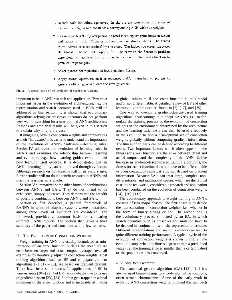
Fig. 2. A typical cycle of the evolution of connection weights.

important tasks in ANN research and application. Two mostimportant issues in the evolution of architectures, i.e., therepresentation and search operators used in EA’s, will beaddressed in this section. It is shown that evolutionaryalgorithms relying on crossover operators do not performvery well in searching for a near-optimal ANN architecture.Reasons and empirical results will be given in this sectionto explain why this is the case.

If imagining ANN’s connection weights and architecturesas their “hardware,” it is easier to understand the importanceof the evolution of ANN’s “software”—learning rules.Section IV addresses the evolution of learning rules inANN’s and examines the relationship between learningand evolution, e.g., how learning guides evolution andhow learning itself evolves. It is demonstrated that anANN’s learning ability can be improved through evolution.Although research on this topic is still in its early stages,further studies will no doubt benefit research in ANN’s andmachine learning as a whole.

Section V summarizes some other forms of combinationsbetween ANN’s and EA’s. They do not intend to beexhaustive, simply indicative. They demonstrate the breadthof possible combinations between ANN’s and EA’s.

Section VI first describes a general framework ofEANN’s in terms of adaptive systems where interactionsamong three levels of evolution are considered. Theframework provides a common basis for comparingdifferent EANN models. The section then gives a briefsummary of the paper and concludes with a few remarks.

II. THE EVOLUTION OF CONNECTION WEIGHTS

Weight training in ANN’s is usually formulated as min-imization of an error function, such as the mean squareerror between target and actual outputs averaged over allexamples, by iteratively adjusting connection weights. Mosttraining algorithms, such as BP and conjugate gradientalgorithms [7], [17]–[19], are based on gradient descent.There have been some successful applications of BP invarious areas [20]–[22], but BP has drawbacks due to its useof gradient descent [23], [24]. It often gets trapped in a localminimum of the error function and is incapable of finding

a global minimum if the error function is multimodaland/or nondifferentiable. A detailed review of BP and otherlearning algorithms can be found in [7], [17], and [25].

One way to overcome gradient-descent-based trainingalgorithms’ shortcomings is to adopt EANN’s, i.e., to for-mulate the training process as the evolution of connectionweights in the environment determined by the architectureand the learning task. EA’s can then be used effectivelyin the evolution to find a near-optimal set of connectionweights globally without computing gradient information.The fitness of an ANN can be defined according to differentneeds. Two important factors which often appear in thefitness (or error) function are the error between target andactual outputs and the complexity of the ANN. Unlikethe case in gradient-descent-based training algorithms, thefitness (or error) function does not have to be differentiableor even continuous since EA’s do not depend on gradientinformation. Because EA’s can treat large, complex, non-differentiable, and multimodal spaces, which are the typicalcase in the real world, considerable research and applicationhas been conducted on the evolution of connection weights[24], [26]–[112].

The evolutionary approach to weight training in ANN’sconsists of two major phases. The first phase is to decidethe representation of connection weights, i.e., whether inthe form of binary strings or not. The second one isthe evolutionary process simulated by an EA, in whichsearch operators such as crossover and mutation have tobe decided in conjunction with the representation scheme.Different representations and search operators can lead toquite different training performance. A typical cycle of theevolution of connection weights is shown in Fig. 2. Theevolution stops when the fitness is greater than a predefinedvalue (i.e., the training error is smaller than a certain value)or the population has converged.

A. Binary Representation

The canonical genetic algorithm (GA) [13], [14] hasalways used binary strings to encode alternative solutions,often termed chromosomes. Some of the early work inevolving ANN connection weights followed this approach

YAO: EVOLVING ARTIFICIAL NEURAL NETWORKS 1425

(a) (b)

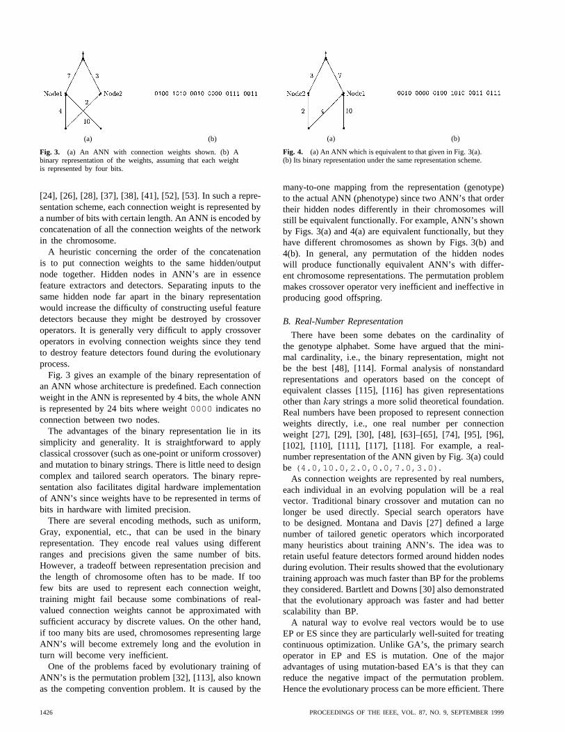
Fig. 3. (a) An ANN with connection weights shown. (b) Abinary representation of the weights, assuming that each weightis represented by four bits.

[24], [26], [28], [37], [38], [41], [52], [53]. In such a repre-sentation scheme, each connection weight is represented bya number of bits with certain length. An ANN is encoded byconcatenation of all the connection weights of the networkin the chromosome.

A heuristic concerning the order of the concatenationis to put connection weights to the same hidden/outputnode together. Hidden nodes in ANN’s are in essencefeature extractors and detectors. Separating inputs to thesame hidden node far apart in the binary representationwould increase the difficulty of constructing useful featuredetectors because they might be destroyed by crossoveroperators. It is generally very difficult to apply crossoveroperators in evolving connection weights since they tendto destroy feature detectors found during the evolutionaryprocess.

Fig. 3 gives an example of the binary representation ofan ANN whose architecture is predefined. Each connectionweight in the ANN is represented by 4 bits, the whole ANNis represented by 24 bits where weight0000 indicates noconnection between two nodes.

The advantages of the binary representation lie in itssimplicity and generality. It is straightforward to applyclassical crossover (such as one-point or uniform crossover)and mutation to binary strings. There is little need to designcomplex and tailored search operators. The binary repre-sentation also facilitates digital hardware implementationof ANN’s since weights have to be represented in terms ofbits in hardware with limited precision.

There are several encoding methods, such as uniform,Gray, exponential, etc., that can be used in the binaryrepresentation. They encode real values using differentranges and precisions given the same number of bits.However, a tradeoff between representation precision andthe length of chromosome often has to be made. If toofew bits are used to represent each connection weight,training might fail because some combinations of real-valued connection weights cannot be approximated withsufficient accuracy by discrete values. On the other hand,if too many bits are used, chromosomes representing largeANN’s will become extremely long and the evolution inturn will become very inefficient.

One of the problems faced by evolutionary training ofANN’s is the permutation problem [32], [113], also knownas the competing convention problem. It is caused by the

(a) (b)

Fig. 4. (a) An ANN which is equivalent to that given in Fig. 3(a).(b) Its binary representation under the same representation scheme.

many-to-one mapping from the representation (genotype)to the actual ANN (phenotype) since two ANN’s that ordertheir hidden nodes differently in their chromosomes willstill be equivalent functionally. For example, ANN’s shownby Figs. 3(a) and 4(a) are equivalent functionally, but theyhave different chromosomes as shown by Figs. 3(b) and4(b). In general, any permutation of the hidden nodeswill produce functionally equivalent ANN’s with differ-ent chromosome representations. The permutation problemmakes crossover operator very inefficient and ineffective inproducing good offspring.

B. Real-Number Representation

There have been some debates on the cardinality ofthe genotype alphabet. Some have argued that the mini-mal cardinality, i.e., the binary representation, might notbe the best [48], [114]. Formal analysis of nonstandardrepresentations and operators based on the concept ofequivalent classes [115], [116] has given representationsother than ary strings a more solid theoretical foundation.Real numbers have been proposed to represent connectionweights directly, i.e., one real number per connectionweight [27], [29], [30], [48], [63]–[65], [74], [95], [96],[102], [110], [111], [117], [118]. For example, a real-number representation of the ANN given by Fig. 3(a) couldbe (4.0,10.0,2.0,0.0,7.0,3.0) .

As connection weights are represented by real numbers,each individual in an evolving population will be a realvector. Traditional binary crossover and mutation can nolonger be used directly. Special search operators haveto be designed. Montana and Davis [27] defined a largenumber of tailored genetic operators which incorporatedmany heuristics about training ANN’s. The idea was toretain useful feature detectors formed around hidden nodesduring evolution. Their results showed that the evolutionarytraining approach was much faster than BP for the problemsthey considered. Bartlett and Downs [30] also demonstratedthat the evolutionary approach was faster and had betterscalability than BP.

A natural way to evolve real vectors would be to useEP or ES since they are particularly well-suited for treatingcontinuous optimization. Unlike GA’s, the primary searchoperator in EP and ES is mutation. One of the majoradvantages of using mutation-based EA’s is that they canreduce the negative impact of the permutation problem.Hence the evolutionary process can be more efficient. There


have been a number of successful examples of applying EPor ES to the evolution of ANN connection weights [29],[63]–[65], [67], [68], [95], [96], [102], [106], [111], [117],[119], [120]. In these examples, the primary search operatorhas been Gaussian mutation. Other mutation operators, suchas Cauchy mutation [121], [122], can also be used. EPand ES also allow self adaptation of strategy parameters.Evolving connection weights by EP can be implementedas follows.

1) Generate an initial population of individuals atrandom and set . Each individual is a pairof real-valued vectors, ,where ’s are connection weight vectors and’s arevariance vectors for Gaussian mutations (also knownas strategy parameters in self-adaptive EA’s). Eachindividual corresponds to an ANN.

2) Each individual , creates asingle offspring by: for

(2)

(3)

where , and denote theth component of the vectors and ,

respectively. denotes a normally distributedone-dimensional random number with mean zero andvariance one. indicates that the randomnumber is generated anew for each value of. Theparameters and are commonly set toand [15], [123]. in (3) may bereplaced by Cauchy mutation [121], [122], [124] forfaster evolution.

3) Determine the fitness of every individual, includingall parents and offspring, based on the training error.Different error functions may be used here.

4) Conduct pairwise comparison over the union of par-ents and offspring .For each individual, opponents are chosen uni-formly at random from all the parents and offspring.For each comparison, if the individual’s fitness isno smaller than the opponent’s, it receives a “win.”Select individuals out of and

, that have most wins to form thenext generation. (This tournament selection schememay be replaced by other selection schemes, such as[125].)

5) Stop if the halting criterion is satisfied; otherwise,and go to Step 2).

C. Comparison Between Evolutionary Trainingand Gradient-Based Training

As indicated at the beginning of Section II, the evolu-tionary training approach is attractive because it can handlethe global search problem better in a vast, complex, mul-timodal, and nondifferentiable surface. It does not dependon gradient information of the error (or fitness) functionand thus is particularly appealing when this information

is unavailable or very costly to obtain or estimate. Forexample, the evolutionary approach has been used to trainrecurrent ANN’s [41], [60], [65], [100], [102], [103], [106],[117], [126]–[128], higher order ANN’s [52], [53], andfuzzy ANN’s [76], [77], [129], [130]. Moreover, the sameEA can be used to train many different networks regardlessof whether they are feedforward, recurrent, or higher orderANN’s. The general applicability of the evolutionary ap-proach saves a lot of human efforts in developing differenttraining algorithms for different types of ANN’s.

The evolutionary approach also makes it easier to gener-ate ANN’s with some special characteristics. For example,the ANN’s complexity can be decreased and its generaliza-tion increased by including a complexity (regularization)term in the fitness function. Unlike the case in gradient-based training, this term does not need to be differentiableor even continuous. Weight sharing and weight decay canalso be incorporated into the fitness function easily.

Evolutionary training can be slow for some problems incomparison with fast variants of BP [131] and conjugategradient algorithms [19], [132]. However, EA’s are gen-erally much less sensitive to initial conditions of training.They always search for a globally optimal solution, whilea gradient descent algorithm can only find a local optimumin a neighborhood of the initial solution.

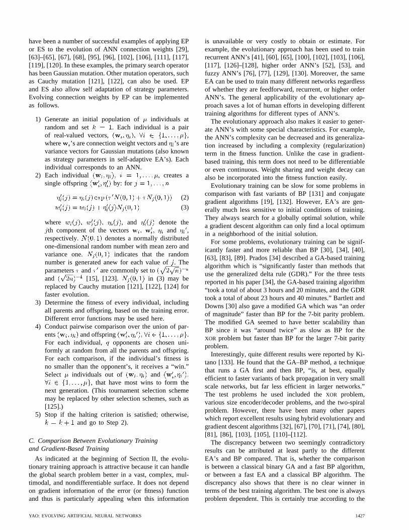
For some problems, evolutionary training can be signif-icantly faster and more reliable than BP [30], [34], [40],[63], [83], [89]. Prados [34] described a GA-based trainingalgorithm which is “significantly faster than methods thatuse the generalized delta rule (GDR).” For the three testsreported in his paper [34], the GA-based training algorithm“took a total of about 3 hours and 20 minutes, and the GDRtook a total of about 23 hours and 40 minutes.” Bartlett andDowns [30] also gave a modified GA which was “an orderof magnitude” faster than BP for the 7-bit parity problem.The modified GA seemed to have better scalability thanBP since it was “around twice” as slow as BP for theXOR problem but faster than BP for the larger 7-bit parityproblem.

Interestingly, quite different results were reported by Ki-tano [133]. He found that the GA–BP method, a techniquethat runs a GA first and then BP, “is, at best, equallyefficient to faster variants of back propagation in very smallscale networks, but far less efficient in larger networks.”The test problems he used included theXOR problem,various size encoder/decoder problems, and the two-spiralproblem. However, there have been many other paperswhich report excellent results using hybrid evolutionary andgradient descent algorithms [32], [67], [70], [71], [74], [80],[81], [86], [103], [105], [110]–[112].

The discrepancy between two seemingly contradictoryresults can be attributed at least partly to the differentEA’s and BP compared. That is, whether the comparisonis between a classical binary GA and a fast BP algorithm,or between a fast EA and a classical BP algorithm. Thediscrepancy also shows that there is no clear winner interms of the best training algorithm. The best one is alwaysproblem dependent. This is certainly true according to the


no-free-lunch theorem [134]. In general, hybrid algorithmstend to perform better than others for a large number ofproblems.

D. Hybrid Training

Most EA’s are rather inefficient in fine-tuned local searchalthough they are good at global search. This is especiallytrue for GA’s. The efficiency of evolutionary training canbe improved significantly by incorporating a local searchprocedure into the evolution, i.e., combining EA’s globalsearch ability with local search’s ability to fine tune. EA’scan be used to locate a good region in the space and thena local search procedure is used to find a near-optimalsolution in this region. The local search algorithm couldbe BP [32], [133] or other random search algorithms [30],[135]. Hybrid training has been used successfully in manyapplication areas [32], [67], [70], [71], [74], [80], [81], [86],[103], [105], [110]–[112].

Lee [81] and many others [32], [136]–[138] used GA’s tosearch for a near-optimal set of initial connection weightsand then used BP to perform local search from theseinitial weights. Their results showed that the hybrid GA/BPapproach was more efficient than either the GA or BP al-gorithm used alone. If we consider that BP often has to runseveral times in practice in order to find good connectionweights due to its sensitivity to initial conditions, the hybridtraining algorithm will be quite competitive. Similar workon the evolution of initial weights has also been done oncompetitive learning neural networks [139] and Kohonennetworks [140].

It is interesting to consider finding good initial weightsas locating a good region in the weight space. Defining thatbasin of attraction of a local minimum as being composedof all the points, sets of weights in this case, which canconverge to the local minimum through a local searchalgorithm, then a global minimum can easily be found bythe local search algorithm if an EA can locate a point, i.e., aset of initial weights, in the basin of attraction of the globalminimum. Fig. 5 illustrates a simple case where there isonly one connection weight in the ANN. If an EA can findan initial weight such as , it would be easy for a localsearch algorithm to arrive at the globally optimal weight

even though itself is not as good as .

III. T HE EVOLUTION OF ARCHITECTURES

Section II assumed that the architecture of an ANN ispredefined and fixed during the evolution of connectionweights. This section discusses the design of ANN architec-tures. The architecture of an ANN includes its topologicalstructure, i.e., connectivity, and the transfer function of eachnode in the ANN. As indicated in the beginning of thispaper, architecture design is crucial in the successful ap-plication of ANN’s because the architecture has significantimpact on a network’s information processing capabilities.Given a learning task, an ANN with only a few connectionsand linear nodes may not be able to perform the taskat all due to its limited capability, while an ANN with

Fig. 5. An illustration of using an EA to find good initial weightssuch that a local search algorithm can find the globally optimalweights easily.wI2 in this figure is an optimal initial weightbecause it can lead to the global optimumwB using a local searchalgorithm.

a large number of connections and nonlinear nodes mayoverfit noise in the training data and fail to have goodgeneralization ability.

Up to now, architecture design is still very much a humanexpert’s job. It depends heavily on the expert experienceand a tedious trial-and-error process. There is no systematicway to design a near-optimal architecture for a given taskautomatically. Research on constructive and destructive al-gorithms represents an effort toward the automatic design ofarchitectures [141]–[148]. Roughly speaking, a constructivealgorithm starts with a minimal network (network withminimal number of hidden layers, nodes, and connections)and adds new layers, nodes, and connections when nec-essary during training while a destructive algorithm doesthe opposite, i.e., starts with the maximal network anddeletes unnecessary layers, nodes, and connections duringtraining. However, as indicated by Angelineet al. [149],“Such structural hill climbing methods are susceptible tobecoming trapped at structural local optima.” In addition,they “only investigate restricted topological subsets ratherthan the complete class of network architectures” [149].

Design of the optimal architecture for an ANN can beformulated as a search problem in the architecture spacewhere each point represents an architecture. Given someperformance (optimality) criteria, e.g., lowest training error,lowest network complexity, etc., about architectures, theperformance level of all architectures forms a discretesurface in the space. The optimal architecture design isequivalent to finding the highest point on this surface. Thereare several characteristics of such a surface as indicated byMiller et al. [150] which make EA’s a better candidate forsearching the surface than those constructive and destruc-tive algorithms mentioned above. These characteristics are[150]:

1) the surface is infinitely large since the number ofpossible nodes and connections is unbounded;

2) the surface is nondifferentiable since changes in thenumber of nodes or connections are discrete and canhave a discontinuous effect on EANN’s performance;


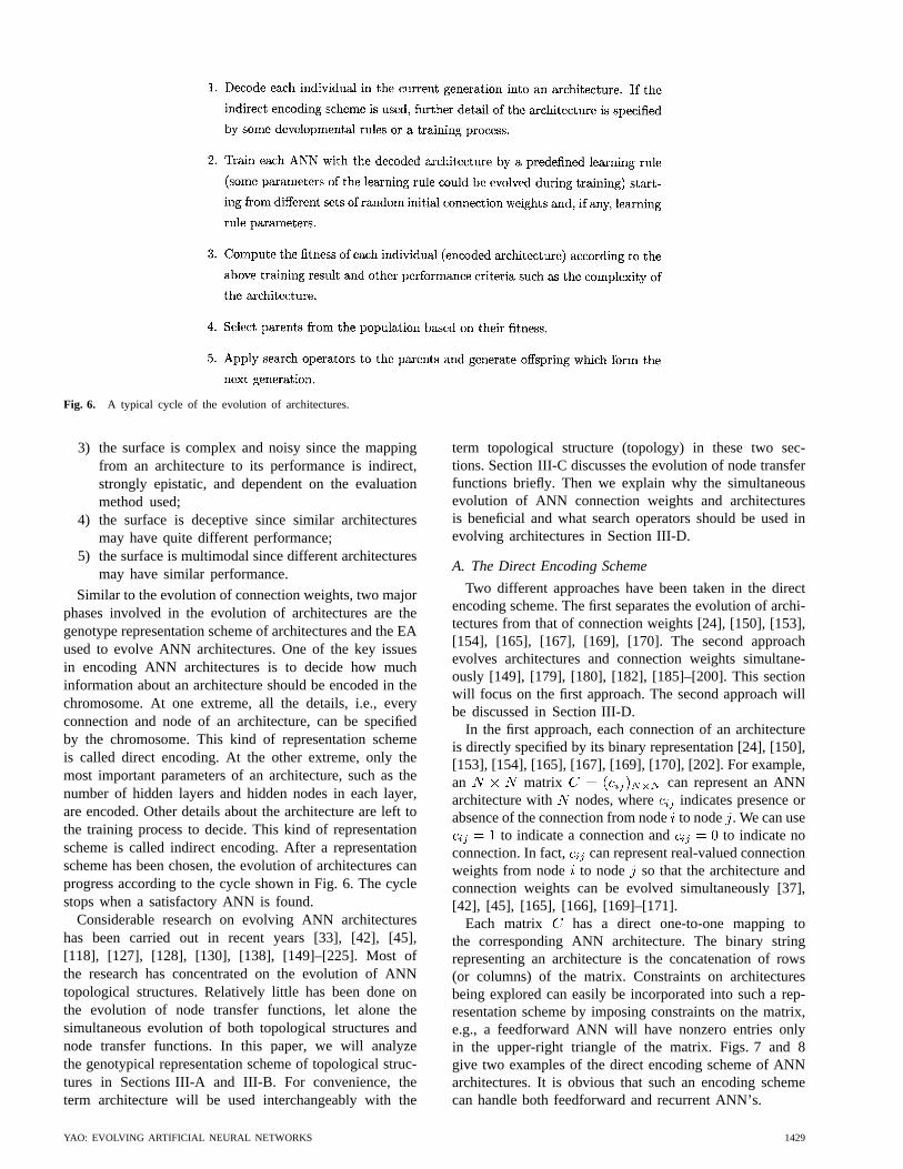
Fig. 6. A typical cycle of the evolution of architectures.

3) the surface is complex and noisy since the mappingfrom an architecture to its performance is indirect,strongly epistatic, and dependent on the evaluationmethod used;

4) the surface is deceptive since similar architecturesmay have quite different performance;

5) the surface is multimodal since different architecturesmay have similar performance.

Similar to the evolution of connection weights, two majorphases involved in the evolution of architectures are thegenotype representation scheme of architectures and the EAused to evolve ANN architectures. One of the key issuesin encoding ANN architectures is to decide how muchinformation about an architecture should be encoded in thechromosome. At one extreme, all the details, i.e., everyconnection and node of an architecture, can be specifiedby the chromosome. This kind of representation schemeis called direct encoding. At the other extreme, only themost important parameters of an architecture, such as thenumber of hidden layers and hidden nodes in each layer,are encoded. Other details about the architecture are left tothe training process to decide. This kind of representationscheme is called indirect encoding. After a representationscheme has been chosen, the evolution of architectures canprogress according to the cycle shown in Fig. 6. The cyclestops when a satisfactory ANN is found.

Considerable research on evolving ANN architectureshas been carried out in recent years [33], [42], [45],[118], [127], [128], [130], [138], [149]–[225]. Most ofthe research has concentrated on the evolution of ANNtopological structures. Relatively little has been done onthe evolution of node transfer functions, let alone thesimultaneous evolution of both topological structures andnode transfer functions. In this paper, we will analyzethe genotypical representation scheme of topological struc-tures in Sections III-A and III-B. For convenience, theterm architecture will be used interchangeably with the

term topological structure (topology) in these two sec-tions. Section III-C discusses the evolution of node transferfunctions briefly. Then we explain why the simultaneousevolution of ANN connection weights and architecturesis beneficial and what search operators should be used inevolving architectures in Section III-D.

A. The Direct Encoding Scheme

Two different approaches have been taken in the directencoding scheme. The first separates the evolution of archi-tectures from that of connection weights [24], [150], [153],[154], [165], [167], [169], [170]. The second approachevolves architectures and connection weights simultane-ously [149], [179], [180], [182], [185]–[200]. This sectionwill focus on the first approach. The second approach willbe discussed in Section III-D.

In the first approach, each connection of an architectureis directly specified by its binary representation [24], [150],[153], [154], [165], [167], [169], [170], [202]. For example,an matrix can represent an ANNarchitecture with nodes, where indicates presence orabsence of the connection from nodeto node . We can use

to indicate a connection and to indicate noconnection. In fact, can represent real-valued connectionweights from node to node so that the architecture andconnection weights can be evolved simultaneously [37],[42], [45], [165], [166], [169]–[171].

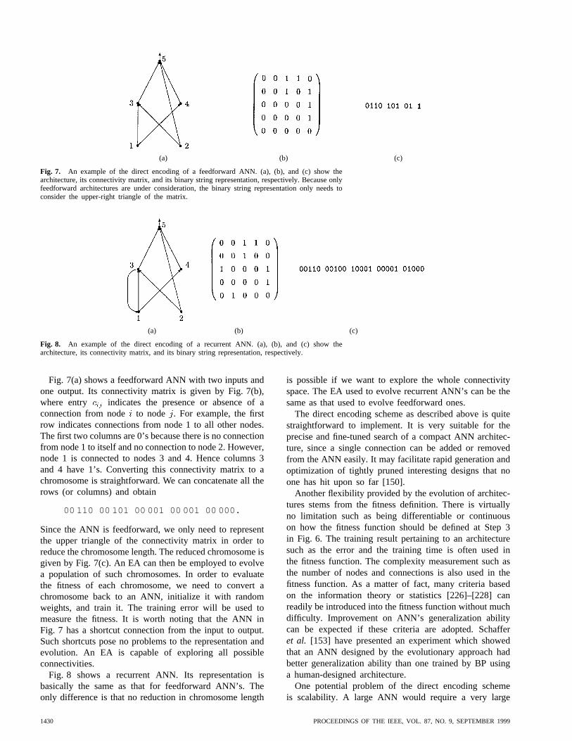
Each matrix has a direct one-to-one mapping tothe corresponding ANN architecture. The binary stringrepresenting an architecture is the concatenation of rows(or columns) of the matrix. Constraints on architecturesbeing explored can easily be incorporated into such a rep-resentation scheme by imposing constraints on the matrix,e.g., a feedforward ANN will have nonzero entries onlyin the upper-right triangle of the matrix. Figs. 7 and 8give two examples of the direct encoding scheme of ANNarchitectures. It is obvious that such an encoding schemecan handle both feedforward and recurrent ANN’s.


(a) (b) (c)

Fig. 7. An example of the direct encoding of a feedforward ANN. (a), (b), and (c) show thearchitecture, its connectivity matrix, and its binary string representation, respectively. Because onlyfeedforward architectures are under consideration, the binary string representation only needs toconsider the upper-right triangle of the matrix.

(a) (b) (c)

Fig. 8. An example of the direct encoding of a recurrent ANN. (a), (b), and (c) show thearchitecture, its connectivity matrix, and its binary string representation, respectively.

Fig. 7(a) shows a feedforward ANN with two inputs andone output. Its connectivity matrix is given by Fig. 7(b),where entry indicates the presence or absence of aconnection from node to node . For example, the firstrow indicates connections from node 1 to all other nodes.The first two columns are 0’s because there is no connectionfrom node 1 to itself and no connection to node 2. However,node 1 is connected to nodes 3 and 4. Hence columns 3and 4 have 1’s. Converting this connectivity matrix to achromosome is straightforward. We can concatenate all therows (or columns) and obtain

00 110 00 101 00 001 00 001 00 000.

Since the ANN is feedforward, we only need to representthe upper triangle of the connectivity matrix in order toreduce the chromosome length. The reduced chromosome isgiven by Fig. 7(c). An EA can then be employed to evolvea population of such chromosomes. In order to evaluatethe fitness of each chromosome, we need to convert achromosome back to an ANN, initialize it with randomweights, and train it. The training error will be used tomeasure the fitness. It is worth noting that the ANN inFig. 7 has a shortcut connection from the input to output.Such shortcuts pose no problems to the representation andevolution. An EA is capable of exploring all possibleconnectivities.

Fig. 8 shows a recurrent ANN. Its representation isbasically the same as that for feedforward ANN’s. Theonly difference is that no reduction in chromosome length

is possible if we want to explore the whole connectivityspace. The EA used to evolve recurrent ANN’s can be thesame as that used to evolve feedforward ones.

The direct encoding scheme as described above is quitestraightforward to implement. It is very suitable for theprecise and fine-tuned search of a compact ANN architec-ture, since a single connection can be added or removedfrom the ANN easily. It may facilitate rapid generation andoptimization of tightly pruned interesting designs that noone has hit upon so far [150].

Another flexibility provided by the evolution of architec-tures stems from the fitness definition. There is virtuallyno limitation such as being differentiable or continuouson how the fitness function should be defined at Step 3in Fig. 6. The training result pertaining to an architecturesuch as the error and the training time is often used inthe fitness function. The complexity measurement such asthe number of nodes and connections is also used in thefitness function. As a matter of fact, many criteria basedon the information theory or statistics [226]–[228] canreadily be introduced into the fitness function without muchdifficulty. Improvement on ANN’s generalization abilitycan be expected if these criteria are adopted. Schafferet al. [153] have presented an experiment which showedthat an ANN designed by the evolutionary approach hadbetter generalization ability than one trained by BP usinga human-designed architecture.

One potential problem of the direct encoding schemeis scalability. A large ANN would require a very large


matrix and thus increase the computation time of theevolution. One way to cut down the size of matrices isto use domain knowledge to reduce the search space. Forexample, if complete connection is to be used between twoneighboring layers in a feedforward ANN, its architecturecan be encoded by just the number of hidden layers andnodes in each hidden layer. The length of chromosome canbe reduced greatly in this case [153], [154]. However, doingso requires sufficient domain knowledge and expertise,which are difficult to obtain in practice. We also run therisk of missing some very good solutions when we restrictthe search space manually.

The permutation problem as illustrated by Figs. 3 and4 in Section II-A still exists and causes unwanted sideeffects in the evolution of architectures. Because two func-tionally equivalent ANN’s which order their hidden nodesdifferently have two different genotypical representations,the probability of producing a highly fit offspring byrecombining them is often very low. Some researchersthus avoided crossover and adopted only mutations inthe evolution of architectures [45], [128], [149], [179],[185]–[197], [217], [223], although it has been shown thatcrossover may be useful and important in increasing theefficiency of evolution for some problems [48], [113],[212], [229]. Hancock [113] suggested that the permutationproblem might “not be as severe as had been supposed”with the population size and the selection mechanism heused because “The increased number of ways of solvingthe problem outweigh the difficulties of bringing buildingblocks together.” Thierens [101] proposed a genetic encod-ing scheme of ANN’s which can avoid the permutationproblem, however, only very limited experimental resultswere presented. It is worth indicating that most studies onthe permutation problem concentrate on the GA used, e.g.,genetic operators, population sizes, selection mechanisms,etc. While it is necessary to investigate the algorithm, it isequally important to study the genotypical representationscheme, since the performance surface defined in the be-ginning of Section III is determined by the representation.More research is needed to further understand the impact ofthe permutation problem on the evolution of architectures.

B. The Indirect Encoding Scheme

In order to reduce the length of the genotypical represen-tation of architectures, the indirect encoding scheme hasbeen used by many researchers [151], [152], [155], [156],[159], [160], [168], [184], [205], [208], [211], [230]–[232]where only some characteristics of an architecture areencoded in the chromosome. The details about each con-nection in an ANN is either predefined according to priorknowledge or specified by a set of deterministic devel-opmental rules. The indirect encoding scheme can pro-duce more compact genotypical representation of ANNarchitectures, but it may not be very good at findinga compact ANN with good generalization ability. Some[151], [230], [231] have argued that the indirect encodingscheme is biologically more plausible than the direct one,because it is impossible for genetic information encoded in

chromosomes to specify independently the whole nervoussystem according to the discoveries of neuroscience.

1) Parametric Representation:ANN architectures maybe specified by a set of parameters such as the numberof hidden layers, the number of hidden nodes in eachlayer, the number of connections between two layers, etc.These parameters can be encoded in various forms in achromosome. Harpet al. [152], [156] used a “blueprint” torepresent an architecture which consists of one or moresegments representing an area (layer) and its efferentconnectivity (projections). The first and last area areconstrained to be the input and output area, respectively.Each segment includes two parts of the information: 1)that about the area itself, such as the number of nodes inthe area and the spatial organization of the area, and 2)that about the efferent connectivity. It should be noted thatonly the connectivity pattern instead of each connectionis specified here. The detailed node-to-node connection isspecified by implicit developmental rules, e.g., the networkinstantiation software used by Harpet al. [152], [156].Similar parametric representation methods with differentsets of parameters have also been proposed by others [155],[159]. An interesting aspect of Harpet al.’s work is theircombination of learning parameters with architectures inthe genotypical representation. The learning parameters canevolve along with architecture parameters. The interactionbetween the two can be explored through evolution.

Although the parametric representation method can re-duce the length of binary chromosome specifying ANN’sarchitectures, EA’s can only search a limited subset ofthe whole feasible architecture space. For example, if weencode only the number of hidden nodes in the hidden layer,we basically assume strictly layered feedforward ANN’swith a single hidden layer. We will have to assume twoneighboring layers are fully connected as well. In general,the parametric representation method will be most suitablewhen we know what kind of architectures we are tryingto find.

2) Developmental Rule Representation:A quite differentindirect encoding method from the above is to encode de-velopmental rules, which are used to construct architectures,in chromosomes [151], [168], [184], [205], [230], [232].The shift from the direct optimization of architectures tothe optimization of developmental rules has brought somebenefits, such as more compact genotypical representation,to the evolution of architectures. The destructive effect ofcrossover will also be lessened since the developmental rulerepresentation is capable of preserving promising buildingblocks found so far [151]. But this method also has someproblems [233].

A developmental rule is usually described by a recursiveequation [230] or a generation rule similar to a productionrule in a production system with a left-hand side (LHS) anda right-hand side (RHS) [151]. The connectivity pattern ofthe architecture in the form of a matrix is constructed from abasis, i.e., a single-element matrix, by repetitively applyingsuitable developmental rules to nonterminal elements in


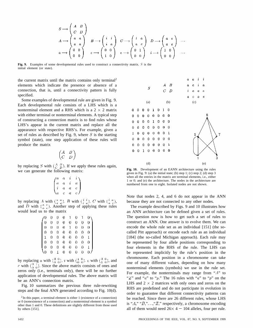
Fig. 9. Examples of some developmental rules used to construct a connectivity matrix.S is theinitial element (or state).

the current matrix until the matrix contains only terminal2

elements which indicate the presence or absence of aconnection, that is, until a connectivity pattern is fullyspecified.

Some examples of developmental rule are given in Fig. 9.Each developmental rule consists of a LHS which is anonterminal element and a RHS which is a 22 matrixwith either terminal or nonterminal elements. A typical stepof constructing a connection matrix is to find rules whoseLHS’s appear in the current matrix and replace all theappearance with respective RHS’s. For example, given aset of rules as described by Fig. 9, whereis the startingsymbol (state), one step application of these rules willproduce the matrix

by replacing with . If we apply these rules again,we can generate the following matrix:

by replacing with with with ,and with . Another step of applying these ruleswould lead us to the matrix

by replacing with with with , andwith . Since the above matrix consists of ones and

zeros only (i.e., terminals only), there will be no furtherapplication of developmental rules. The above matrix willbe an ANN’s connection matrix.

Fig. 10 summarizes the previous three rule-rewritingsteps and the final ANN generated according to Fig. 10(d).

2In this paper, a terminal element is either 1 (existence of a connection)or 0 (nonexistence of a connection) and a nonterminal element is a symbolother than 1 and 0. These definitions are slightly different from those usedby others [151].

(a) (b) (c)

(d) (e)

Fig. 10. Development of an EANN architecture using the rulesgiven in Fig. 9: (a) the initial state; (b) step 1; (c) step 2; (d) step 3when all the entries in the matrix are terminal elements, i.e., either1 or 0; and (e) the architecture. The nodes in the architecture arenumbered from one to eight. Isolated nodes are not shown.

Note that nodes 2, 4, and 6 do not appear in the ANNbecause they are not connected to any other nodes.

The example described by Figs. 9 and 10 illustrates howan ANN architecture can be defined given a set of rules.The question now is how to get such a set of rules toconstruct an ANN. One answer is to evolve them. We canencode the whole rule set as an individual [151] (the so-called Pitt approach) or encode each rule as an individual[184] (the so-called Michigan approach). Each rule maybe represented by four allele positions corresponding tofour elements in the RHS of the rule. The LHS canbe represented implicitly by the rule’s position in thechromosome. Each position in a chromosome can takeone of many different values, depending on how manynonterminal elements (symbols) we use in the rule set.For example, the nonterminals may range from “” to“ ” and “ ” to “ .” The 16 rules with “ ” to “ ” on theLHS and 2 2 matrices with only ones and zeros on theRHS are predefined and do not participate in evolution inorder to guarantee that different connectivity patterns canbe reached. Since there are 26 different rules, whose LHSis “ ,” “ ,” ,“ ,” respectively, a chromosome encodingall of them would need 26 4 104 alleles, four per rule.


The LHS of a rule is implicitly determined by its positionin the chromosome. For example, the rule set in Fig. 9 canbe represented by the following chromosome:

ABCDaaaaiiiaiaacaeaewhere the first four elements indicate the RHS of rule “”,the second four indicate the RHS of rule “,” etc.

Some good results from the developmental rule repre-sentation method have been reported [151] using varioussize encoder/decoder problems. However, the method hassome limitations. It often needs to predefine the number ofrewriting steps. It does not allow recursive rules. It is notvery good at evolving detailed connectivity patterns amongindividual nodes. A compact genotypical representationdoes not imply a compact phenotypical representation, i.e.,a compact ANN architecture. Recent work by Siddiqi andLucas [233] shows that the direct encoding scheme can beat least as good as the developmental rule method. Theyhave reimplemented Kitano’s system and discovered thatthe performance difference between the direct and indirectencoding schemes was not caused by the encoding schemeitself, but by how sparsely connected the initial ANNarchitectures were in the initial population [151]. The directencoding scheme achieved the same performance as thatachieved by the developmental rule representation whenthe initial conditions were the same [233].

The developmental rule representation method normallyseparates the evolution of architectures from that of con-nection weights. This creates some problems for evolution.Section III-D will discuss these in more detail.

Mjolsnesset al. [230] described a similar rule encodingmethod where rules are represented by recursive equa-tions which specify the growth of connection matrices.Coefficients of these recursive equations, represented bydecomposition matrices, are encoded in genotypes and op-timized by simulated annealing instead of EA’s. Connectionweights are optimized along with connectivity by simulatedannealing since each entry of a connection matrix can havea real-valued weight. One advantage of using simulatedannealing instead of GA’s in the evolution is the avoidanceof the destructive effect of crossover. Wilson [234] alsoused simulated annealing in ANN architecture design.

3) Fractal Representation:Merrill and Port [231] pro-posed another method for encoding architectures whichis based on the use of fractal subsets of the plane. Theyargued that the fractal representation of architectures wasbiologically more plausible than the developmental rulerepresentation. They used three real-valued parameters, i.e.,an edge code, an input coefficient, and an output coefficientto specify each node in an architecture. In a sense, thisencoding method is closer to the direct encoding schemerather to the indirect one. Fast simulated annealing [235]was used in the evolution.

4) Other Representations:A very different approach tothe evolution of architectures has been proposed by Ander-sen and Tsoi [236]. Their approach is unique in that eachindividual in a population represents a hidden node ratherthan the whole architecture. An architecture is built layerby layer, i.e., hidden layers are added one by one if the

current architecture cannot reduce the training error belowcertain threshold. Each hidden layer is constructed auto-matically through an evolutionary process which employsthe GA with fitness sharing. Fitness sharing encourages theformation of different feature detectors (hidden nodes) inthe population. The number of hidden nodes in each hiddenlayer can vary.

One limitation of this approach [236] is that it couldonly deal with strictly layered feedforward ANN’s. Anotherlimitation is that there are usually several hidden nodes inthe same species which have very similar functionality,i.e., which are basically the same feature detector in apopulation. Such redundancy needs to be removed by anadditional clean-up algorithm.

Smith and Cribbs [181], [237] also used an individualto represent a hidden node rather than the whole ANN.Their approach can only deal with strictly three-layeredfeedforward ANN’s.

C. The Evolution of Node Transfer Functions

The discussion on the evolution of architectures so faronly deals with the topological structure of an architecture.The transfer function of each node in the architecture hasbeen assumed to be fixed and predefined by human experts,yet the transfer function has been shown to be an importantpart of an ANN architecture and have significant impact onANN’s performance [238]–[240]. The transfer function isoften assumed to be the same for all the nodes in an ANN,at least for all the nodes in the same layer.

Storket al. [241] were, to our best knowledge, the first toapply EA’s to the evolution of both topological structuresand node transfer functions even though only simple ANN’swith seven nodes were considered. The transfer functionwas specified in the structural genes in their genotypicrepresentation. It was much more complex than the usualsigmoid function because they tried to model a biologicalneuron in the tailflip circuitry of crayfish.

White and Ligomenides [171] adopted a simpler ap-proach to the evolution of both topological structures andnode transfer functions. For each individual (i.e., ANN)in the initial population, 80% nodes in the ANN usedthe sigmoid transfer function and 20% nodes used theGaussian transfer function. The evolution was used todecide the optimal mixture between these two transferfunctions automatically. The sigmoid and Gaussian transferfunction themselves were not evolvable. No parameters ofthe two functions were evolved.

Liu and Yao [191] used EP to evolve ANN’s withboth sigmoidal and Gaussian nodes. Rather than fixingthe total number of nodes and evolve mixture of differentnodes, their algorithm allowed growth and shrinking of thewhole ANN by adding or deleting a node (either sigmoidalor Gaussian). The type of node added or deleted wasdetermined at random. Good performance was reported forsome benchmark problems [191]. Hwanget al. [225] wentone step further. They evolved ANN topology, node transferfunction, as well as connection weights for projection neuralnetworks.


Sebald and Chellapilla [242] used the evolution of nodetransfer function as an example to show the importance ofevolving representations. Representation and search are thetwo key issues in problem solving. Co-evolving solutionsand their representations may be an effective way to tacklesome difficult problems where little human expertise isavailable.

D. Simultaneous Evolution of Architecturesand Connection Weights

The evolutionary approaches discussed so far in design-ing ANN architectures evolve architectures only, withoutany connection weights. Connection weights have to belearned after a near-optimal architecture is found. This is es-pecially true if one uses the indirect encoding scheme, suchas the developmental rule method. One major problem withthe evolution of architectures without connection weightsis noisy fitness evaluation [194]. In other words, fitnessevaluation as described in step 3 of Fig. 6 is very inaccurateand noisy because a phenotype’s (i.e., an ANN with afull set of weights) fitness was used to approximate itsgenotype’s (i.e., an ANN without any weight information)fitness. There are two major sources of noise [194].

1) The first source is the random initialization of theweights. Different random initial weights may pro-duce different training results. Hence, the same geno-type may have quite different fitness due to differentrandom initial weights used in training.

2) The second source is the training algorithm. Differenttraining algorithms may produce different trainingresults even from the same set of initial weights. Thisis especially true for multimodal error functions. Forexample, BP may reduce an ANN’s error to 0.05through training, but an EA could reduce the errorto 0.001 due to its global search capability.

Such noise may mislead evolution because the fact thatthe fitness of a phenotype generated from genotypeishigher than that generated from genotypedoes not meanthat truly has higher quality than . In order to reducesuch noise, an architecture usually has to be trained manytimes from different random initial weights. The averageresult is then used to estimate the genotype’s mean fitness.This method increases the computation time for fitnessevaluation dramatically. It is one of the major reasons whyonly small ANN’s were evolved in previous studies.

In essence, the noise identified in this paper is caused bythe one-to-many mapping from genotypes to phenotypes.Angelineet al. [149] and Fogel [12], [243] have provided amore general discussion on the mapping between genotypesand phenotypes. It is clear that the evolution of architectureswithout any weight information has difficulties in evaluat-ing fitness accurately. As a result, the evolution would bevery inefficient.

One way to alleviate this problem is to evolve ANNarchitectures and connection weights simultaneously [37],[42], [45], [149], [165], [166], [169]–[172], [179], [180],

[182], [185]–[200], [230], [232]. In this case, each individ-ual in a population is a fully specified ANN with completeweight information. Since there is a one-to-one mappingbetween a genotype and its phenotype, fitness evaluationis accurate.

One issue in evolving ANN’s is the choice of searchoperators used in EA’s. Both crossover-based and mutation-based EA’s have been used. However, use of crossoverappears to contradict the basic ideas behind ANN’s, becausecrossover works best when there exist “building blocks” butit is unclear what a building block might be in an ANN sinceANN’s emphasize distributed (knowledge) representation[244]. The knowledge in an ANN is distributed among allthe weights in the ANN. Recombining one part of an ANNwith another part of another ANN is likely to destroy bothANN’s.

However, if ANN’s do not use a distributed represen-tation but rather a localized one, such as radial basisfunction (RBF) networks or nearest-neighbor multilayerperceptrons, crossover might be a very useful operator.There has been some work in this area where good resultswere reported [119], [120], [245]–[253]. In general, ANN’susing distributed representation are more compact and havebetter generalization capability for most practical problems.

Yao and Liu [193], [194] developed an automatic system,EPNet, based on EP for simultaneous evolution of ANNarchitectures and connection weights. EPNet does not useany crossover operators for the reason given above. It relieson a number of mutation operators to modify architecturesand weights. Behavioral (i.e., functional) evolution, rathergenetic evolution, is emphasized in EPNet. A number oftechniques were adopted to maintain the behavioral linkbetween a parent and its offspring [190]. Fig. 11 shows themain structure of EPNet.

EPNet uses rank-based selection [125] and five muta-tions: hybrid training; node deletion; connection deletion;connection addition; and node addition [188], [194], [254].Hybrid training is the only mutation in EPNet which mod-ifies ANN’s weights. It is based on a modified BP (MBP)algorithm with an adaptive learning rate and simulatedannealing. The other four mutations are used to grow andprune hidden nodes and connections.

The number of epochs used by MBP to train each ANN’sin a population is defined by two user-specified parameters.There is no guarantee that an ANN will converge to evena local optimum after those epochs. Hence this trainingprocess is called partial training. It is used to bridge thebehavioral gap between a parent and its offspring.

The five mutations are attempted sequentially. If onemutation leads to a better offspring, it is regarded assuccessful. No further mutation will be applied. Otherwisethe next mutation is attempted. The motivation behindordering mutations is to encourage the evolution of compactANN’s without sacrificing generalization. A validation setis used in EPNet to measure the fitness of an individual.

EPNet has been tested extensively on a number of bench-mark problems and achieved excellent results, includingparity problems of size from four to eight, the two-spiral


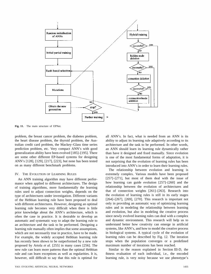
Fig. 11. The main structure of EPNet.

problem, the breast cancer problem, the diabetes problem,the heart disease problem, the thyroid problem, the Aus-tralian credit card problem, the Mackey–Glass time seriesprediction problem, etc. Very compact ANN’s with goodgeneralization ability have been evolved [185]–[195]. Thereare some other different EP-based systems for designingANN’s [128], [129], [217], [223], but none has been testedon as many different benchmark problems.

IV. THE EVOLUTION OF LEARNING RULES

An ANN training algorithm may have different perfor-mance when applied to different architectures. The designof training algorithms, more fundamentally the learningrules used to adjust connection weights, depends on thetype of architectures under investigation. Different variantsof the Hebbian learning rule have been proposed to dealwith different architectures. However, designing an optimallearning rule becomes very difficult when there is littleprior knowledge about the ANN’s architecture, which isoften the case in practice. It is desirable to develop anautomatic and systematic way to adapt the learning rule toan architecture and the task to be performed. Designing alearning rule manually often implies that some assumptions,which are not necessarily true in practice, have to be made.For example, the widely accepted Hebbian learning rulehas recently been shown to be outperformed by a new ruleproposed by Artolaet al. [255] in many cases [256]. Thenew rule can learn more patterns than the optimal Hebbianrule and can learn exceptions as well as regularities. It is,however, still difficult to say that this rule is optimal for

all ANN’s. In fact, what is needed from an ANN is itsability to adjust its learning rule adaptively according to itsarchitecture and the task to be performed. In other words,an ANN should learn its learning rule dynamically ratherthan have it designed and fixed manually. Since evolutionis one of the most fundamental forms of adaptation, it isnot surprising that the evolution of learning rules has beenintroduced into ANN’s in order to learn their learning rules.

The relationship between evolution and learning isextremely complex. Various models have been proposed[257]–[271], but most of them deal with the issue ofhow learning can guide evolution [257]–[260] and therelationship between the evolution of architectures andthat of connection weights [261]–[263]. Research intothe evolution of learning rules is still in its early stages[264]–[267], [269], [270]. This research is important notonly in providing an automatic way of optimizing learningrules and in modeling the relationship between learningand evolution, but also in modeling the creative processsince newly evolved learning rules can deal with a complexand dynamic environment. This research will help us tounderstand better how creativity can emerge in artificialsystems, like ANN’s, and how to model the creative processin biological systems. A typical cycle of the evolution oflearning rules can be described by Fig. 12. The iterationstops when the population converges or a predefinedmaximum number of iterations has been reached.

Similar to the reason explained in Section III-D, thefitness evaluation of each individual, i.e., the encodedlearning rule, is very noisy because we use phenotype’s


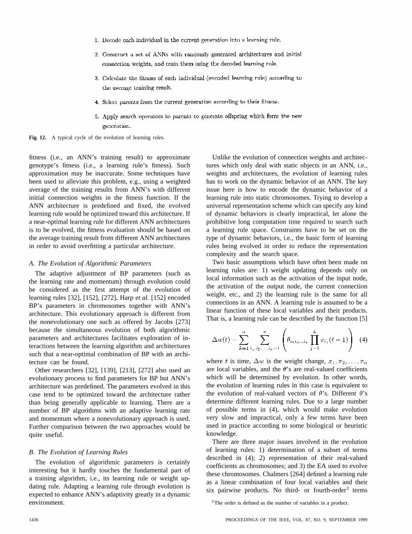
Fig. 12. A typical cycle of the evolution of learning rules.

fitness (i.e., an ANN’s training result) to approximategenotype’s fitness (i.e., a learning rule’s fitness). Suchapproximation may be inaccurate. Some techniques havebeen used to alleviate this problem, e.g., using a weightedaverage of the training results from ANN’s with differentinitial connection weights in the fitness function. If theANN architecture is predefined and fixed, the evolvedlearning rule would be optimized toward this architecture. Ifa near-optimal learning rule for different ANN architecturesis to be evolved, the fitness evaluation should be based onthe average training result from different ANN architecturesin order to avoid overfitting a particular architecture.

A. The Evolution of Algorithmic Parameters

The adaptive adjustment of BP parameters (such asthe learning rate and momentum) through evolution couldbe considered as the first attempt of the evolution oflearning rules [32], [152], [272]. Harpet al. [152] encodedBP’s parameters in chromosomes together with ANN’sarchitecture. This evolutionary approach is different fromthe nonevolutionary one such as offered by Jacobs [273]because the simultaneous evolution of both algorithmicparameters and architectures facilitates exploration of in-teractions between the learning algorithm and architecturessuch that a near-optimal combination of BP with an archi-tecture can be found.

Other researchers [32], [139], [213], [272] also used anevolutionary process to find parameters for BP but ANN’sarchitecture was predefined. The parameters evolved in thiscase tend to be optimized toward the architecture ratherthan being generally applicable to learning. There are anumber of BP algorithms with an adaptive learning rateand momentum where a nonevolutionary approach is used.Further comparison between the two approaches would bequite useful.

B. The Evolution of Learning Rules

The evolution of algorithmic parameters is certainlyinteresting but it hardly touches the fundamental part ofa training algorithm, i.e., its learning rule or weight up-dating rule. Adapting a learning rule through evolution isexpected to enhance ANN’s adaptivity greatly in a dynamicenvironment.

Unlike the evolution of connection weights and architec-tures which only deal with static objects in an ANN, i.e.,weights and architectures, the evolution of learning ruleshas to work on the dynamic behavior of an ANN. The keyissue here is how to encode the dynamic behavior of alearning rule into static chromosomes. Trying to develop auniversal representation scheme which can specify any kindof dynamic behaviors is clearly impractical, let alone theprohibitive long computation time required to search sucha learning rule space. Constraints have to be set on thetype of dynamic behaviors, i.e., the basic form of learningrules being evolved in order to reduce the representationcomplexity and the search space.

Two basic assumptions which have often been made onlearning rules are: 1) weight updating depends only onlocal information such as the activation of the input node,the activation of the output node, the current connectionweight, etc., and 2) the learning rule is the same for allconnections in an ANN. A learning rule is assumed to be alinear function of these local variables and their products.That is, a learning rule can be described by the function [5]

(4)

where is time, is the weight change,are local variables, and the’s are real-valued coefficientswhich will be determined by evolution. In other words,the evolution of learning rules in this case is equivalent tothe evolution of real-valued vectors of’s. Different ’sdetermine different learning rules. Due to a large numberof possible terms in (4), which would make evolutionvery slow and impractical, only a few terms have beenused in practice according to some biological or heuristicknowledge.

There are three major issues involved in the evolutionof learning rules: 1) determination of a subset of termsdescribed in (4); 2) representation of their real-valuedcoefficients as chromosomes; and 3) the EA used to evolvethese chromosomes. Chalmers [264] defined a learning ruleas a linear combination of four local variables and theirsix pairwise products. No third- or fourth-order3 terms

3The order is defined as the number of variables in a product.


were used. Ten coefficients and a scale parameter wereencoded in a binary string via exponential encoding. Thearchitecture used in the fitness evaluation was fixed becauseonly single-layer ANN’s were considered and the numberof inputs and outputs were fixed by the learning task athand. After 1000 generations, starting from a population ofrandomly generated learning rules, the evolution discoveredthe well-known delta rule [7], [274] and some of its vari-ants. These experiments, although simple and preliminary,demonstrated the potential of evolution in discovering novellearning rules from a set of randomly generated rules.However, constraints set on learning rules could preventsome from being evolved such as those which include third-or fourth-order terms.

Similar experiments on the evolution of learning ruleswere also carried out by others [265], [266], [267], [269],[270]. Fontanari and Meir [267] used Chalmers’ approachto evolve learning rules for binary perceptrons. They alsoconsidered four local variables but only seven terms wereadopted in their learning rules, which included one first-order, three second-order, and three third-order terms in (4).Baxter [269] took one step further than just the evolutionof learning rules. He tried to evolve complete ANN’s(including connection weights, architectures, and learningrules) in a single level of evolution. It is clear that the searchspace of possible ANN’s would be enormous if constraintswere not set on the connection weights, architectures, andlearning rules. In his experiments, only ANN’s with binarythreshold nodes were considered, so the weights could onlybe 1 or 1. The number of nodes in ANN’s was fixed.The learning rule only considered two Boolean variables.Although Baxter’s experiments were rather simple, theyconfirmed that complex behaviors could be learned andthe ANN’s learning ability could be improved throughevolution [269].

Bengioet al.’s approach [265], [266] is slightly differentfrom Chalmers’ in the sense that gradient descent algo-rithms and simulated annealing, rather than EA’s, wereused to find near-optimal’s. In their experiments, fourlocal variables and one zeroth-order, three first-order, andthree second-order terms in (4) were used.

Research related to the evolution of learning rules in-cludes Parisiet al.’s work on “econets,” although theydid not evolve learning rules explicitly [260], [275]. Theyemphasized the crucial role of the environment in whichthe evolution occured while only using some simple neuralnetworks. The issue of environmental diversity is closelyrelated to the noisy fitness evaluation as pointed out inSection III-D and at the beginning of Section IV. Thereare two possible sources of noise. The first is the decodingprocess (morphogenesis) of chromosomes. The second isintroduced when a decoded learning rule is evaluated byusing it to train ANN’s. The environmental diversity isessential in obtaining a good approximation to the fitnessof the decoded learning rule and thus in reducing the noisefrom the second source. If a general learning rule whichis applicable to a wide range of ANN architectures andlearning tasks is needed, the environmental diversity has to

be very high, i.e., many different architectures and learningtasks have to be used in the fitness evaluation.

V. OTHER COMBINATIONS BETWEEN ANN’ S AND EA’S

A. The Evolution of Input Features

For many practical problems, the possible inputs to anANN can be quite large. There may be some redundancyamong different inputs. A large number of inputs to anANN increase its size and thus require more training dataand longer training times in order to achieve a reasonablegeneralization ability. Preprocessing is often needed toreduce the number of inputs to an ANN. Various dimensionreduction techniques, including the principal componentanalysis, have been used for this purpose.

The problem of finding a near-optimal set of inputfeatures to an ANN can be formulated as a search problem.Given a large set of potential inputs, we want to find a near-optimal subset which has the fewest number of featuresbut the performance of the ANN using this subset is noworse than that of the ANN using the whole input set. EA’shave been used to perform such a search effectively [267],[277]–[287]. Very good results, i.e., better performancewith fewer inputs, have been reported from these studies.In the evolution of input features, each individual in thepopulation represents a subset of all possible inputs. Thiscan be implemented using a binary chromosome whoselength is the same as the total number of input features.Each bit in the chromosome corresponds to a feature. “1”indicates presence of a feature, while “0” indicates absenceof the feature. The evaluation of an individual is carried outby training an ANN with these inputs and using the resultto calculate its fitness value. The ANN architecture is oftenfixed. Such evaluation is very noisy, however, because ofthe reason explained in Section III-D.

Not only does the evolution of input features provide away to discover important features from all possible inputsautomatically, it can also be used to discover new trainingexamples. Zhang and Veenker [288] described an activelearning paradigm where a training algorithm based onEA’s can self-select training examples. Cho and Cha [289]proposed another algorithm for evolving training sets byadding virtual samples.

B. ANN as Fitness Estimator

EA’s have been used with success to optimize variouscontrol parameters [290]–[292]. However, it is very timeconsuming and costly to obtain fitness values for somecontrol problems as it is impractical to run a real systemfor each combination of control parameters. In order toget around this problem and make evolution more efficient,fitness values are often approximated rather than computedexactly. ANN’s are often used to model and approximatea real control system due to their good generalizationabilities. The input to such ANN’s will be a set of controlparameters. The output will be the control system outputfrom which an evaluation of the whole system can easily be


obtained. When an EA is used to search for a near-optimalset of control parameters, the ANN will be used in fitnessevaluation rather than the real control system [293]–[297].

This combination of ANN’s and EA’s has a couple ofadvantages in evolving control systems. First, the time-consuming fitness evaluation based on real control systemsis replaced by fast fitness evaluation based on ANN’s. Sec-ond, this combination provides safer evolution of controlsystems. EA’s are stochastic algorithms. It is possible thatsome poor control parameters may be generated in theevolutionary process. These parameters could damage areal control system. If we use ANN’s to estimate fitness,we do not need to use the real system and thus can avoiddamages to the real system. However, how successful thiscombination approach will be depends largely on how wellANN’s learn and generalize.

C. Evolving ANN Ensembles

Learning is often formulated as an optimization problemin the machine learning field. However, learning is differentfrom optimization in practice because we want the learnedsystem to have best generalization, which is different fromminimizing an error function on a training data set. TheANN with the minimum error on a training data set maynot have best generalization unless there is an equivalencebetween generalization and the error on the training data.Unfortunately, measuring generalization quantitatively andaccurately is almost impossible in practice [298] althoughthere are many theories and criteria on generalization,such as the minimum description length (MDL) [299],Akaike information criteria (AIC) [300], and minimummessage length (MML) [301]. In practice, these criteriaare often used to define better error functions in the hopethat minimizing the functions will maximize generalization.While these functions often lead to better generalization oflearned systems, there is no guarantee.

EA’s are often used to maximize a fitness function orminimize an error function, and thus they face the sameproblem as described above: maximizing a fitness functionis different from maximizing generalization. The EA isactually used as an optimization, not learning, algorithm.While little can be done for traditional nonpopulation-basedlearning, there are opportunities for improving population-based learning, e.g., evolutionary learning.

Since the maximum fitness may not be equivalent to bestgeneralization in evolutionary learning, the best individualwith the maximum fitness in a population may not bethe one we want. Other individuals in the population maycontain some useful information that will help to improvegeneralization of learned systems. It is thus beneficialto make use of the whole population rather than anysingle individual. A population always contains at leastas much information as any single individual. Hence,combining different individuals in the population to forman integrated system is expected to produce better results.Such a population of ANN’s is called an ANN ensemblein this section. There have been some very successful

experiments which show that EA’s can be used to evolveANN ensembles [192], [193], [302]–[305].

D. Others

There are some other novel combinations betweenANN’s and EA’s. For example, Zitar and Hassoun [306]used EA’s to extract rules in a reinforcement learningsystem and then used them to train ANN’s. Sziranyi[99] and Pal and Bhandari [98] used EA’s to tune circuitparameters and templates in cellular ANN’s. Olmez [97]used EA’s to optimize a modified restricted Coulombenergy (RCE) ANN. Imada and Araki [307] used EA’sto evolve connection weights for Hopfield ANN’s. Manyothers used EA’s and ANN’s for combinatorial or global(numerical) optimization in order to combine EA’s globalsearch capability with ANN’s fast convergence to localoptima [308]–[318].

VI. CONCLUDING REMARKS

Although evolution has been introduced into ANN’s atvarious levels, they can roughly be divided into three: theevolution of connection weights, architectures, and learningrules. This section first describes a general framework forANN’s and then draws some conclusions.

A. A General Framework for EANN’s

A general framework for EANN’s can be describedby Fig. 13 [3]–[5]. The evolution of connection weightsproceeds at the lowest level on the fastest time scale in anenvironment determined by an architecture, a learning rule,and learning tasks. There are, however, two alternatives todecide the level of the evolution of architectures and that oflearning rules: either the evolution of architectures is at thehighest level and that of learning rules at the lower levelor vice versa. The lower the level of evolution, the fasterthe time scale it is on.

From the engineering perspective, the decision on thelevel of evolution depends on what kind of prior knowledgeis available. If there is more prior knowledge about anANN’s architecture than that about their learning rules, orif a particular class of architectures is pursued, it is betterto put the evolution of architectures at the highest levelbecause such knowledge can be encoded in an architecture’sgenotypic representation to reduce the (architecture) searchspace and the lower-level evolution of learning rules canbe biased toward this type of architectures. On the otherhand, the evolution of learning rules should be at thehighest level if there is more prior knowledge about themavailable or if there is a special interest in certain type oflearning rules. Unfortunately, there is usually little priorknowledge available about either architectures or learningrules in practice except for some very vague statements[319]. In this case, it is more appropriate to put the evolutionof architectures at the highest level since the optimalityof a learning rule makes more sense when evaluated inan environment including the architecture to which the


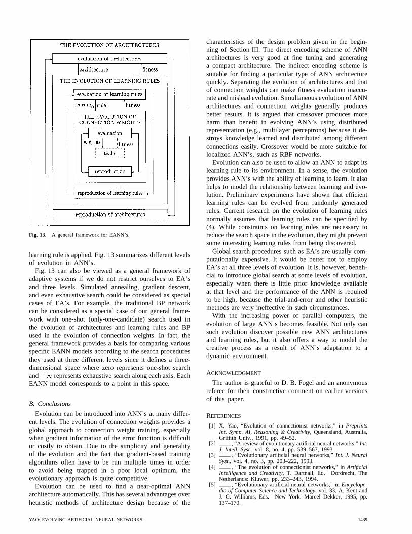
Fig. 13. A general framework for EANN’s.

learning rule is applied. Fig. 13 summarizes different levelsof evolution in ANN’s.

Fig. 13 can also be viewed as a general framework ofadaptive systems if we do not restrict ourselves to EA’sand three levels. Simulated annealing, gradient descent,and even exhaustive search could be considered as specialcases of EA’s. For example, the traditional BP networkcan be considered as a special case of our general frame-work with one-shot (only-one-candidate) search used inthe evolution of architectures and learning rules and BPused in the evolution of connection weights. In fact, thegeneral framework provides a basis for comparing variousspecific EANN models according to the search proceduresthey used at three different levels since it defines a three-dimensional space where zero represents one-shot searchand represents exhaustive search along each axis. EachEANN model corresponds to a point in this space.

B. Conclusions

Evolution can be introduced into ANN’s at many differ-ent levels. The evolution of connection weights provides aglobal approach to connection weight training, especiallywhen gradient information of the error function is difficultor costly to obtain. Due to the simplicity and generalityof the evolution and the fact that gradient-based trainingalgorithms often have to be run multiple times in orderto avoid being trapped in a poor local optimum, theevolutionary approach is quite competitive.

Evolution can be used to find a near-optimal ANNarchitecture automatically. This has several advantages overheuristic methods of architecture design because of the

characteristics of the design problem given in the begin-ning of Section III. The direct encoding scheme of ANNarchitectures is very good at fine tuning and generatinga compact architecture. The indirect encoding scheme issuitable for finding a particular type of ANN architecturequickly. Separating the evolution of architectures and thatof connection weights can make fitness evaluation inaccu-rate and mislead evolution. Simultaneous evolution of ANNarchitectures and connection weights generally producesbetter results. It is argued that crossover produces moreharm than benefit in evolving ANN’s using distributedrepresentation (e.g., multilayer perceptrons) because it de-stroys knowledge learned and distributed among differentconnections easily. Crossover would be more suitable forlocalized ANN’s, such as RBF networks.

Evolution can also be used to allow an ANN to adapt itslearning rule to its environment. In a sense, the evolutionprovides ANN’s with the ability of learning to learn. It alsohelps to model the relationship between learning and evo-lution. Preliminary experiments have shown that efficientlearning rules can be evolved from randomly generatedrules. Current research on the evolution of learning rulesnormally assumes that learning rules can be specified by(4). While constraints on learning rules are necessary toreduce the search space in the evolution, they might preventsome interesting learning rules from being discovered.

Global search procedures such as EA’s are usually com-putationally expensive. It would be better not to employEA’s at all three levels of evolution. It is, however, benefi-cial to introduce global search at some levels of evolution,especially when there is little prior knowledge availableat that level and the performance of the ANN is requiredto be high, because the trial-and-error and other heuristicmethods are very ineffective in such circumstances.

With the increasing power of parallel computers, theevolution of large ANN’s becomes feasible. Not only cansuch evolution discover possible new ANN architecturesand learning rules, but it also offers a way to model thecreative process as a result of ANN’s adaptation to adynamic environment.

ACKNOWLEDGMENT

The author is grateful to D. B. Fogel and an anonymousreferee for their constructive comment on earlier versionsof this paper.

REFERENCES

[1] X. Yao, “Evolution of connectionist networks,” inPreprintsInt. Symp. AI, Reasoning & Creativity, Queensland, Australia,Griffith Univ., 1991, pp. 49–52.

[2] , “A review of evolutionary artificial neural networks,”Int.J. Intell. Syst., vol. 8, no. 4, pp. 539–567, 1993.

[3] , “Evolutionary artificial neural networks,”Int. J. NeuralSyst., vol. 4, no. 3, pp. 203–222, 1993.

[4] , “The evolution of connectionist networks,” inArtificialIntelligence and Creativity, T. Dartnall, Ed. Dordrecht, TheNetherlands: Kluwer, pp. 233–243, 1994.

[5] , “Evolutionary artificial neural networks,” inEncyclope-dia of Computer Science and Technology, vol. 33, A. Kent andJ. G. Williams, Eds. New York: Marcel Dekker, 1995, pp.137–170.


[6] G. E. Hinton, “Connectionist learning procedures,”ArtificialIntell., vol. 40, no. 1–3, pp. 185–234, Sept. 1989.

[7] J. Hertz, A. Krogh, and R. Palmer,Introduction to the Theory ofNeural Computation. Reading, MA: Addison-Wesley, 1991.

[8] H.-P. Schwefel,Numerical Optimization of Computer Models.Chichester, U.K.: Wiley, 1981.

[9] H.-P. Schwefel,Evolution and Optimum Seeking. New York:Wiley, 1995.

[10] L. J. Fogel, A. J. Owens, and M. J. Walsh,Artificial IntelligenceThrough Simulated Evolution. New York: Wiley, 1966.

[11] D. B. Fogel, System Identification Through Simulated Evolu-tion: A Machine Learning Approach to Modeling. NeedhamHeights, MA: Ginn, 1991.

[12] , Evolutionary Computation: Toward a New Philosophy ofMachine Intelligence. New York: IEEE Press, 1995.

[13] J. H. Holland, Adaptation in Natural and Artificial Systems.Ann Arbor, MI: Univ. Michigan Press, 1975.

[14] D. E. Goldberg,Genetic Algorithms in Search, Optimization,and Machine Learning. Reading, MA: Addison-Wesley, 1989.

[15] D. B. Fogel, “An introduction to simulated evolutionary opti-mization,” IEEE Trans. Neural Networks, vol. 5, pp. 3–14, Jan.1994.

[16] T. Back, U. Hammel, and H.-P. Schwefel, “Evolutionary com-putation: Comments on the history and current state,”IEEETrans. Evolutionary Computation, vol. 1, pp. 3–17, Apr. 1997.

[17] D. R. Hush and B. G. Horne, “Progress in supervised neuralnetworks,” IEEE Signal Processing Mag., vol. 10, pp. 8–39,Jan. 1993.

[18] D. E. Rumelhart, G. E. Hinton, and R. J. Williams, “Learn-ing internal representations by error propagation,” inParallelDistributed Processing: Explorations in the Microstructures ofCognition, vol. I, D. E. Rumelhart and J. L. McClelland, Eds.Cambridge, MA: MIT Press, 1986, pp. 318–362.

[19] M. F. Møller, “A scaled conjugate gradient algorithm forfast supervised learning,”Neural Networks, vol. 6, no. 4, pp.525–533, 1993.

[20] K. J. Lang, A. H. Waibel, and G. E. Hinton, “A time-delayneural network architecture for isolated word recognition,”Neural Networks, vol. 3, no. 1, pp. 33–43, 1990.

[21] S. S. Fels and G. E. Hinton, “Glove-talk: A neural networkinterface between a data-glove and a speech synthesizer,”IEEETrans. Neural Networks, vol. 4, pp. 2–8, Jan. 1993.

[22] S. Knerr, L. Personnaz, and G. Dreyfus, “Handwritten digitrecognition by neural networks with single-layer training,”IEEE Trans. Neural Networks, vol. 3, pp. 962–968, Nov. 1992.

[23] R. S. Sutton, “Two problems with backpropagation and othersteepest-descent learning procedures for networks,” inProc.8th Annual Conf. Cognitive Science Society. Hillsdale, NJ:Erlbaum, 1986, pp. 823–831.

[24] D. Whitley, T. Starkweather, and C. Bogart, “Genetic al-gorithms and neural networks: Optimizing connections andconnectivity,” Parallel Comput., vol. 14, no. 3, pp. 347–361,1990.

[25] Y. Chauvin and D. E. Rumelhart, Eds.,Backpropagation: The-ory, Architectures, and Applications. Hillsdale, NJ: Erlbaum,1995.

[26] D. Whitley, “The GENITOR algorithm and selective pressure:Why rank-based allocation of reproductive trials is best,” inProc. 3rd Int. Conf. Genetic Algorithms and Their Applications,J. D. Schaffer, Ed. San Mateo, CA: Morgan Kaufmann, 1989,pp. 116–121.

[27] D. Montana and L. Davis, “Training feedforward neural net-works using genetic algorithms,” inProc. 11th Int. Joint Conf.Artificial Intelligence. San Mateo, CA: Morgan Kaufmann,1989, pp. 762–767.

[28] T. P. Caudell and C. P. Dolan, “Parametric connectivity:Training of constrained networks using genetic algorithms,” inProc. 3rd Int. Conf. Genetic Algorithms and Their Applications,J. D. Schaffer, Ed. San Mateo, CA: Morgan Kaufmann, 1989,pp. 370–374.

[29] D. B. Fogel, L. J. Fogel, and V. W. Porto, “Evolving neuralnetworks,” Biological Cybern., vol. 63, no. 6, pp. 487–493,1990.

[30] P. Bartlett and T. Downs, “Training a neural network witha genetic algorithm,” Dep. Elect. Eng., Univ. Queensland,Australia, Tech. Rep., Jan. 1990.

[31] J. Heistermann and H. Eckardt, “Parallel algorithms for learningin neural networks with evolution strategy,” inProc. Parallel

Computing’89, D. J. Evans, G. R. Joubert, and F. J. Peters, Eds.Amsterdam, The Netherlands: Elsevier, 1989, pp. 275–280.

[32] R. K. Belew, J. McInerney, and N. N. Schraudolph, “Evolvingnetworks: Using genetic algorithm with connectionist learning,”Comput. Sci. Eng. Dep. (C-014), , Univ. of California, SanDiego, Tech. Rep. CS90-174 (revised), Feb. 1991.

[33] N. J. Radcliffe, “Genetic neural networks on MIMD comput-ers (compressed edition),” Ph.D. dissertation, Dep. TheoreticalPhys., Univ. Edinburgh, U.K., 1990.

[34] D. L. Prados, “Training multilayered neural networks by replac-ing the least fit hidden neurons,” inProc. IEEE SOUTHEAST-CON’92, vol. 2, pp. 634–637.

[35] H. de Garis, “Steerable genNets: The genetic programmingof steerable behaviors in genNets,” inToward a Practice ofAutonomous Systems: Proc. 1st Europ. Conf. Artificial Life, F.J. Varela and P. Bourgine, Eds. Cambridge, MA: MIT Press,1991, pp. 272–281.

[36] , “Using the genetic algorithm to train time dependentbehaviors in neural networks,” inProc. 1st Int. Workshop Mul-tistrategy Learning (MSL-91), R. S. Michalski and G. Tecuci,Eds. Fairfax, VA: Center for Artificial Intelligence, 1991, pp.273–280.

[37] M. Srinivas and L. M. Patnaik, “Learning neural networkweights using genetic algorithms—Improving performance bysearch-space reduction,” inProc. 1991 IEEE Int. Joint Conf.Neural Networks (IJCNN’91 Singapore), vol. 3, pp. 2331–2336.

[38] H. de Garis, “GenNets: Genetically programmed neuralnets—Using the genetic algorithm to train neural nets whoseinputs and/or outputs vary in time,” inProc. 1991 IEEE Int.Joint Conf. Neural Networks (IJCNN’91 Singapore), vol. 2, pp.1391–1396.

[39] A. Homaifar and S. Guan, “Training weights of neural networksby genetic algorithms and messy genetic algorithms,” inProc.2nd IASTED Int. Symp. Expert Systems and Neural Networks,M. H. Hamza, Ed. Anaheim, CA: Acta, 1990, pp. 74–77.

[40] D. L. Prados, “New learning algorithm for training multilay-ered neural networks that uses genetic-algorithm techniques,”Electron. Lett., vol. 28, pp. 1560–1561, July 1992.

[41] A. P. Wieland, “Evolving neural network controllers for un-stable systems,” inProc. 1991 IEEE Int. Joint Conf. NeuralNetworks (IJCNN’91 Seattle), vol. 2, pp. 667–673.

[42] J. R. Koza and J. P. Rice, “Genetic generation of both theweights and architecture for a neural network,” inProc. 1991IEEE Int. Joint Conf. Neural Networks (IJCNN’91 Seattle), vol.2, pp. 397–404.

[43] S. Dominic, R. Das, D. Whitley, and C. Anderson, “Geneticreinforcement learning for neural networks,” inProc. 1991IEEE Int. Joint Conf. Neural Networks (IJCNN’91 Seattle), vol.2, pp. 71–76.

[44] F. A. Dill and B. C. Deer, “An exploration of genetic algorithmsfor the selection of connection weights in dynamical neural net-works,” in Proc. IEEE 1991 National Aerospace and ElectronicsConf. NAECON 1991, vol. 3, pp. 1111–1115.

[45] S. Bornholdt and D. Graudenz, “General asymmetric neuralnetworks and structure design by genetic algorithms,”NeuralNetworks, vol. 5, no. 2, pp. 327–334, 1992.

[46] B. Maricic, “Genetically programmed neural network forsolving pole-balancing problem,” inArtificial Neural Networks:Proc. Int. Conf. Artificial Neural Networks—ICANN-91, vol.2, T. Kohonen, K. Makisara, O. Simula, and J. Kangas,Eds. Amsterdam, The Netherlands: North-Holland, 1991,pp. 1273–1276.

[47] J. J. Spofford and K. J. Hintz, “Evolving sequential machinesin amorphous neural networks,” inArtificial Neural Networks:Proc. Int. Conf. Artificial Neural Networks—ICANN-91, vol. 1,T. Kohonen, K. Makisara, O. Simula, and J. Kangas, Eds. Am-sterdam, The Netherlands: North-Holland, 1991, pp. 973–978.

[48] F. Menczer and D. Parisi, “Evidence of hyperplanes in thegenetic learning of neural networks,”Biological Cybern., vol.66, pp. 283–289, 1992.

[49] Y. Ichikawa and T. Sawa, “Neural network application for directfeedback controllers,”IEEE Trans. Neural Networks, vol. 3, pp.224–231, Mar. 1992.

[50] A. W. O’Neil, “Genetic based training of two-layer, optoelec-tronic neural network,”Electron. Lett., vol. 28, pp. 47–48, Jan.1992.

[51] J. Heistermann, “A mixed genetic approach to the optimizationof neural controllers,” inProc. CompEuro’92, P. Dewilde and J.


Vandewallele, Eds. Los Alamitos, CA: IEEE Computer Soc.,1992, pp. 459–464.

[52] D. J. Janson and J. F. Frenzel, “Application of genetic algo-rithms to the training of higher order neural networks,”J. Syst.Eng., vol. 2, pp. 272–276, 1992.

[53] D. J. Janson and J. F. Frenzel, “Training product unit neuralnetworks with genetic algorithms,”IEEE Expert, vol. 8, pp.26–33, May 1993.

[54] A. V. Scherf and L. D. Voelz, “Training neural networks withgenetic algorithms for target detection,” inProc. SPIE, Conf.Science of Artificial Neural Networks, vol. 1710, pt. 1, Orlando,FL, 1992, pp. 734–741.

[55] E. DeRouin and J. Brown, “Alternative learning methods fortraining neural network classifiers,” inProc. SPIE, Conf. Sci-ence of Artificial Neural Networks, pt. 1, vol. 1710, Orlando,FL, 1992, pp. 474–483.

[56] M. A. Lewis, A. H. Fagg, and A. Solidum, “Genetic pro-gramming approach to the construction of a neural networkfor control of a walking robot,” inProc. 1992 IEEE Int. Conf.Robotics and Automation, vol. 3. Los Alamitos, CA: IEEEComputer Soc., 1992, pp. 2618–2623.

[57] H. B. Penfold, O. F. Diessel, and M. W. Bentink, “A geneticbreeding algorithm which exhibits self-organizing in neuralnetworks,” in Proc. IASTED Int. Symp. Artificial IntelligenceApplication and Neural Networks—AINN’90, M. H. Hamza, Ed.Anaheim, CA: ACTA, 1990, pp. 293–296.

[58] M. L. Gargano, R. A. Marose, and L. von Kleeck, “Anapplication of artificial neural networks and genetic algorithmsto personnel selection in the financial industry,” inProc. 1st Int.Conf. Artificial Intelligence on Wall Street. Los Alamitos, CA:IEEE Computer Soc., 1991, pp. 257–262.

[59] J. G. Elias, “Genetic generation of connection patterns for a dy-namic artificial neural network,” inProc. Int. Workshop Combi-nations of Genetic Algorithms and Neural Networks (COGANN-92), D. Whitley and J. D. Schaffer, Eds. Los Alamitos, CA:IEEE Computer Soc., 1992, pp. 38–54.

[60] R. D. Beer and J. C. Gallagher, “Evolving dynamical neuralnetworks for adaptive behavior,”Adaptive Behavior, vol. 1, no.1, pp. 91–122, 1992.

[61] L. Meeden, “Incremental approach to developing intelligentneural network controllers for robots,”IEEE Trans. Syst., Man,Cybern. B, vol. 26, pp. 474–485, Mar. 1996.

[62] S. Baluja, “Evolution of an artificial neural network basedautonomous land vehicle controller,”IEEE Trans. Syst., Man,Cybern. B, vol. 26, pp. 450–463, Mar. 1996.

[63] V. W. Porto, D. B. Fogel, and L. J. Fogel, “Alternative neuralnetwork training methods,”IEEE Expert, vol. 10, pp. 16–22,Mar. 1995.

[64] S. Yao, C. J. Wei, and Z. Y. He, “Evolving wavelet neuralnetworks for function approximation,”Electron. Lett., vol. 32,no. 4, pp. 360–361, 1996.

[65] G. W. Greenwood, “Training partially recurrent neural net-works using evolutionary strategies,”IEEE Trans. Speech AudioProcessing, vol. 5, pp. 192–194, Feb. 1997.

[66] A. Chilingarian, S. Ter-Antonyan, and A. Vardanyan, “Com-parison of Bayesian and neural techniques in problems ofclassification to multiple categories,”Nuclear Instrum. Methodsin Phys. Res., Section A: Accelerators, Spectrometers, Detectorsand Associated Equipment, vol. 389, nos. 1–2, pp. 230–232,1997.

[67] A. P. Topchy and O. A. Lebedko, “Neural network training bymeans of cooperative evolutionary search,”Nuclear Instrum.Methods in Phys. Res., Section A: Accelerators, Spectrometers,Detectors and Associated Equipment, vol. 389, nos. 1–2, pp.240–241, 1997.

[68] R. Berlich and M. Kunze, “Comparison between the perfor-mance of feed forward neural networks and the supervisedgrowing neural gas algorithm,”Nuclear Instrum. Methods inPhys. Res., Section A: Accelerators, Spectrometers, Detectorsand Associated Equipment, vol. 389, nos. 1–2, pp. 274–277,1997.

[69] Y. Ikuno, H. Kawabata, Y. Hirao, M. Hirata, T. Nagahara, andY. Inagaki, “Application of an improved genetic algorithm tothe learning of neural networks,”Solid State Commun., vol. 91,no. 3, pp. 731–735, 1994.

[70] W. Kinnebrock, “Accelerating the standard backpropagationmethod using a genetic approach,”Neurocomput., vol. 6, nos.5–6, pp. 583–588, 1994.

[71] S. L. Hung and H. Adeli, “Parallel genetic/neural networklearning algorithm for MIMD shared memory machines,”IEEETrans. Neural Networks, vol. 5, pp. 900–909, Nov. 1994.

[72] T. Maifeld and G. Sheble, “Short-term load forecasting by aneural network and a refined genetic algorithm,”Electric PowerSyst. Res., vol. 31, no. 3, pp. 147–152, 1994.

[73] B. Deo, A. Datta, B. Kukreja, R. Rastogi, and K. Deb, “Opti-mization of back propagation algorithm and GAS-assisted ANNmodels for hot metal desulphurization,”Steel Res., vol. 65, no.12, pp. 528–533, 1994.

[74] A. J. Skinner and J. Q. Broughton, “Neural networks in compu-tational materials science: Training algorithms,”Modeling andSimulation in Materials Sci. Eng., vol. 3, no. 3, pp. 371–390,1995.

[75] Y. Chen, M. Narita, and T. Yamada, “Nuclear reactor diagnosticsystem using genetic algorithm (GA)-trained neural networks,”Elect. Eng. Japan (English Translation of Denki Gakkai Ron-bunshi), vol. 115, no. 5, pp. 88–99, 1995.

[76] M. Lehotsky, V. Olej, and J. Chmurny, “Pattern recognitionbased on the fuzzy neural networks and their learning bymodified genetic algorithms,”Neural Network World, vol. 5,no. 1, pp. 91–97, 1995.

[77] N. Wang, D. Yao, and F. Zhang, “Genetic-based fuzzy netcontroller and its application,”Advances in Modeling and Anal.B, vol. 38, nos. 1–2, pp. 49–58, 1997.

[78] P. Osmera, “Optimization of neural networks by genetic al-gorithms,” Neural Network World, vol. 5, no. 6, pp. 965–976,1995.

[79] S. Jain, P.-Y. Peng, A. Tzes, and F. Khorrami, “Neural networkdesign with genetic learning for control of a single link flexiblemanipulator,”J. Intell. Robot. Syst.: Theory Applicat., vol. 15,no. 2, pp. 135–151, 1996.

[80] M. A. Taha and A. S. Hanna, “Evolutionary neural networkmodel for the selection of pavement maintenance strategy,”Transportation Res. Rec., vol. 1497, pp. 70–76, May 1995.

[81] S.-W. Lee, “Off-line recognition of totally unconstrained hand-written numerals using multilayer cluster neural network,”IEEETrans. Pattern Anal. Machine Intell., vol. 18, pp. 648–652, June1996.

[82] S.-K. Lee and D. Jang, “Translation, rotation and scale invariantpattern recognition using spectral analysis and hybrid genetic-neural-fuzzy networks,”Comput. Ind. Eng., vol. 30, no. 3, pp.511–522, 1996.

[83] J. V. Hansen and R. D. Meservy, “Learning experiments withgenetic optimization of a generalized regression neural net-work,” Decision Support Syst., vol. 18, nos. 3–4, pp. 317–325,1996.

[84] S.-J. Huang and C.-L. Huang, “Genetic-based multilayered per-ceptron for Taiwan power system short-term load forecasting,”Electric Power Syst. Res., vol. 38, no. 1, pp. 69–74, 1996.

[85] , “Application of genetic-based neural networks to ther-mal unit commitment,”IEEE Trans. Power Syst., vol. 12, pp.654–660, Feb. 1997.

[86] Y. M. Chen and R. M. O’Connell, “Active power line con-ditioner with a neural network control,”IEEE Trans. Ind.Applicat., vol. 33, pp. 1131–1136, July/Aug. 1997.

[87] C. R. Chen and C. H. Chu, “Concurrent training algorithm forsupervised learning in artificial neural networks,”J. Inform. Sci.Eng., vol. 13, no. 2, pp. 267–291, 1997.

[88] J. Jarmulak, P. Spronck, and E. J. H. Kerckhoffs, “Neuralnetworks in process control: Model-based and reinforcementtrained controllers,”Comput. Electron. Agriculture, vol. 18, nos.2–3, pp. 149–166, 1997.

[89] R. S. Sexton, R. E. Dorsey, and J. D. Johnson, “Toward globaloptimization of neural networks: A comparison of the geneticalgorithm and backpropagation,”Decision Support Syst., vol.22, no. 2, pp. 171–185, 1998.

[90] M. Kamo, T. Kubo, and Y. Iwasa, “Neural network for femalemate preference, trained by a genetic algorithm,”PhilosophicalTrans. Roy. Soc., vol. 353, no. 1367, p. 399, 1998.

[91] J. Zhou and D. L. Civco, “Using genetic learning neuralnetworks for spatial decision making in GIS,”PE & RS:Photogrammetric Eng. Remote Sensing, vol. 62, no. 11, pp.1287–1295, 1996.

[92] B. Yoon, D. J. Holmes, and G. Langholz, “Efficient geneticalgorithms for training layered feedforward neural networks,”Inform. Sci., vol. 76, nos. 1–2, pp. 67–85, 1994.

[93] P. G. Korning, “Training neural networks by means of genetic


algorithms working on very long chromosomes,”Int. J. NeuralSyst., vol. 6, no. 3, pp. 299–316, 1995.

[94] S. Park, L.-J. Park, and C. Park, “A neuro-genetic controller fornonminimum phase systems,”IEEE Trans. Neural Networks,vol. 6, pp. 1297–1300, Sept. 1995.

[95] D. B. Fogel, E. C. Wasson, and V. W. Porto, “A step towardcomputer-assisted mammography using evolutionary program-ming and neural networks,”Cancer Lett., vol. 119, no. 1, p.93, 1997.

[96] D. B. Fogel, E. C. Wasson, and E. M. Boughton, “Evolvingneural networks for detecting breast cancer,”Cancer Lett., vol.96, no. 1, pp. 49–53, 1995.

[97] T. Olmez, “Classification of EEG waveforms by using RCEneural networks and genetic algorithms,”Electron. Lett., vol.33, no. 18, pp. 1561–1562, 1997.

[98] S. Pal and D. Bhandari, “Genetic algorithms with fuzzy fitnessfunction for object extraction using cellular networks,”FuzzySets and Syst., vol. 65, nos. 2–3, pp. 129–139, 1994.

[99] T. Sziranyi, “Robustness of cellular neural networks in imagedeblurring and texture segmentation,”Int. J. Circuit TheoryApplicat., pt 2, vol. 24, no. 3, pp. 381–396, 1996.

[100] P. Adamidis and V. Petridis, “Co-operating populations withdifferent evolution behaviors,” inProc. 1996 IEEE Int. Conf.Evolutionary Computation, ICEC’96, pp. 188–191.

[101] D. Thierens, “Non-redundant genetic coding of neural net-works,” in Proc. 1996 IEEE Int. Conf. Evolutionary Compu-tation, ICEC’96, pp. 571–575.

[102] R. G. Hutchins, “Identifying nonlinear dynamic systems usingneural nets and evolutionary programming,” inProc. 28thAsilomar Conf. Signals, Systems & Computers. Part 2 (of 2).Los Alamitos, CA: IEEE Computer Soc., 1994, pp. 887–891.

[103] J. Lei, G. He, and J.-P. Jiang, “State estimation of the CSTRsystem based on a recurrent neural network trained by HGA’s,”in Proc. 1997 IEEE Int. Conf. Neural Networks. Part 2 (of 4),pp. 779–782.

[104] D. Popvic and K. C. S. Murty, “Retaining diversity of searchpoint distribution through a breeder genetic algorithm for neu-ral network learning,” inProc. 1997 IEEE Int. Conf. NeuralNetworks. Part 1 (of 4), pp. 495–498.

[105] A. Likartsis, I. Vlachavas, and L. H. Tsoukalas, “New hybridneural-genetic methodology for improving learning,” inProc.9th IEEE Int. Conf. Tools with Artificial Intelligence, pp. 32–36.

[106] A. Schultz and H. Wechsler, “Data fusion in neural networksvia computational evolution,” inProc. 1994 IEEE Int. Conf.Neural Networks. Part 5 (of 7), pp. 3044–3049.

[107] M. Koeppen, M. Teunis, and B. Nickolay, “Neural networkthat uses evolutionary learning,” inProc. 1997 IEEE Int. Conf.Evolutionary Computation, ICEC’97, pp. 635–639.

[108] J. Aguilar and A. Colmenares, “Recognition algorithm usingevolutionary learning on the random neural networks,” inProc.1997 IEEE Int. Conf. Neural Networks. Part 2 (of 4), pp.1023–1028.

[109] R. Hochman, T. M. Khoshgoftaar, E. B. Allen, and J. P.Hudepohl, “Evolutionary neural networks: A robust approachto software reliability problems,” inProc. 1997 8th Int. Symp.Software Reliability Engineering. Los Alamitos, CA: IEEEComputer Soc., 1997, pp. 13–26.

[110] W. Yan, Z. Zhu, and R. Hu, “Hybrid genetic/BP algorithm andits application for radar target classification,” inProc. 1997IEEE National Aerospace and Electronics Conf., NAECON. Part2 (of 2), pp. 981–984.

[111] J.-M. Yang, C.-Y. Kao, and J.-T. Horng, “Evolving neuralinduction regular language using combined evolutionaryalgorithms,” in Proc. 1996 1st Joint Conf. Intelligent Sys-tems/ISAI/IFIS, pp. 162–169.

[112] P. Zhang, Y. Sankai, and M. Ohta, “Hybrid adaptive learningcontrol of nonlinear system,” inProc. 1995 American ControlConf. Part 4 (of 6), pp. 2744–2748.

[113] P. J. B. Hancock, “Genetic algorithms and permutation prob-lems: A comparison of recombination operators for neural netstructure specification,” inProc. Int. Workshop Combinationsof Genetic Algorithms and Neural Networks (COGANN-92), D.Whitley and J. D. Schaffer, Eds. Los Alamitos, CA: IEEEComputer Soc., 1992, pp. 108–122.

[114] J. Antonisse, “A new interpretation of schema notation thatoverturns the binary encoding constraint,” inProc. 3rd Int. Conf.Genetic Algorithms and Their Applications, J. D. Schaffer, Ed.San Mateo, CA: Morgan Kaufmann, 1989, pp. 86–91.

[115] N. J. Radcliffe, “Equivalence class analysis of genetic algo-rithms,” Complex Syst., vol. 5, no. 2, pp. 183–205, 1991.

[116] D. B. Fogel and A. Ghozeil, “A note on representations andvariation operators,”IEEE Trans. Evolutionary Computation,vol. 1, pp. 159–161, July 1997.

[117] N. Saravanan and D. B. Fogel, “Evolving neural control sys-tems,” IEEE Expert, vol. 10, pp. 23–27, Mar. 1995.

[118] K. S. Tang, C. Y. Chan, K. F. Man, and S. Kwong, “Geneticstructure for NN topology and weights optimization,” inProc.1st IEE/IEEE Int. Conf. Genetic Algorithms in Engineering Sys-tems: Innovations and Applications (GALESIA’95), Stevenage,U.K., Inst. Elect. Eng. Conf. Pub. 414, pp. 250–255.

[119] M. Sarkar and B. Yegnanarayana, “Evolutionary programming-based probabilistic neural networks construction technique,” inProc. 1997 IEEE Int. Conf. Neural Networks, Part 1 (of 4), pp.456–461.

[120] P. J. Angeline, “Evolving basis functions with dynamic recep-tive fields,” in Proc. 1997 IEEE Int. Conf. Systems, Man, andCybernetics, Part 5 (of 5), pp. 4109–4114.

[121] X. Yao and Y. Liu, “Fast evolutionary programming,” inEvo-lutionary Programming V: Proc. 5th Annu. Conf. EvolutionaryProgramming, L. J. Fogel, P. J. Angeline, and T. Back, Eds.Cambridge, MA: MIT Press, 1996, pp. 451–460.

[122] X. Yao, G. Lin, and Y. Liu, “An analysis of evolutionaryalgorithms based on neighborhood and step sizes,” inEvolu-tionary Programming VI: Proc. 6th Annu. Conf. EvolutionaryProgramming, vol. 1213 ofLecture Notes in Computer Science,P. J. Angeline, R. G. Reynolds, J. R. McDonnell, and R.Eberhart, Eds. Berlin, Germany: Springer-Verlag, 1997, pp.297–307.

[123] T. Back and H.-P. Schwefel, “An overview of evolutionaryalgorithms for parameter optimization,”Evolutionary Compu-tation, vol. 1, no. 1, pp. 1–23, 1993.

[124] X. Yao and Y. Liu, “Fast evolution strategies,”Control Cybern.,vol. 26, no. 3, pp. 467–496, 1997.

[125] X. Yao, “An empirical study of genetic operators in geneticalgorithms,”Microprocessing and Microprogramming, vol. 38,no. 1–5, pp. 707–714, Sept. 1993.

[126] J. Torreele, “Temporal processing with recurrent networks:An evolutionary approach,” inProc. 4th Int. Conf. GeneticAlgorithms, R. K. Belew and L. B. Booker, Eds. San Mateo,CA: Morgan Kaufmann, 1991, pp. 555–561.

[127] M. Mandischer, “Evolving recurrent neural networks with non-binary encoding,” inProc. 1995 IEEE Int. Conf. EvolutionaryComputation, Part 2 (of 2), pp. 584–589.

[128] F. Heimes, G. Zalesski, W. L. Jr., and M. Oshima, “Traditionaland evolved dynamic neural networks for aircraft simulation,”in Proc. 1997 IEEE Int. Conf. Systems, Man, and Cybernetics,Part 3 (of 5), pp. 1995–2000.

[129] K.-H. Wu, C.-H. Chen, and J.-D. Lee, “Cache-genetic-basedmodular fuzzy neural network for robot path planning,” inProc.1996 IEEE Int. Conf. Systems, Man and Cybernetics, Part 4 (of4), pp. 3089–3094, 1996.

[130] T. Ichimura, T. Takano, and E. Tazaki, “Reasoning and learningmethod for fuzzy rules using neural networks with adaptivestructured genetic algorithm,” inProc. 1995 IEEE Int. Conf.Systems, Man and Cybernetics, Part 4 (of 5), pp. 3269–3274.

[131] S. E. Fahlman, “Faster-learning variations on back-propagation:An empirical study,” inProc. 1988 Connectionist Models Sum-mer School, D. S. Touretzky, G. E. Hinton, and T. J. Sejnowski,Eds. San Mateo, CA: Morgan Kaufmann, 1988, pp. 38–51.

[132] E. M. Johansson, F. U. Dowla, and D. M. Goodman, “Backprop-agation learning for multilayer feed-forward neural networksusing the conjugate gradient method,”Int. J. Neural Syst., vol.2, no. 4, pp. 291–301, 1991.

[133] H. Kitano, “Empirical studies on the speed of convergence ofneural network training using genetic algorithms,” inProc. 8thNat. Conf. AI (AAAI-90). Cambridge, MA: MIT Press, 1990,pp. 789–795.

[134] D. H. Wolpert and W. G. Macready, “No free lunch theoremsfor optimization,” IEEE Trans. Evolutionary Computation, vol.1, pp. 67–82, Apr. 1997.

[135] X. Yao, “Optimization by genetic annealing,” inProc. 2ndAustralian Conf. Neural Networks, Sydney, Australia, 1991, pp.94–97.

[136] S. Omatu and S. Deris, “Stabilization of inverted pendulumby the genetic algorithm,” inProc. 1996 IEEE Conf. EmergingTechnologies and Factory Automation, ETFA’96. Part 1 (of 2),


pp. 282–287.[137] S. Omatu and M. Yoshioka, “Self-tuning neuro-PID control and

applications,” inProc. 1997 IEEE Int. Conf. Systems, Man, andCybernetics, Part 3 (of 5), pp. 1985–1989.

[138] I. Erkmen and A. Ozdogan, “Short term load forecasting usinggenetically optimized neural network cascaded with a modifiedKohonen clustering process,” inProc. 1997 IEEE Int. Symp.Intelligent Control, pp. 107–112.

[139] J. J. Merelo, M. Paton, A. Canas, A. Prieto, and F. Moran,“Optimization of a competitive learning neural network bygenetic algorithms,” inProc. Int. Workshop Artificial NeuralNetworks (IWANN’93), Lecture Notes in Computer Science, vol.686. Berlin, Germany: Springer-Verlag, 1993, pp. 185–192.

[140] D. D. Wang and J. Xu, “Fault detection based on evolving LVQneural networks,” inProc. 1996 IEEE Int. Conf. Systems, Manand Cybernetics, vol. 1, pp. 255–260.

[141] S. E. Fahlman and C. Lebiere, “The cascade-correlation learningarchitecture,” inAdvances in Neural Information ProcessingSystems 2, D. S. Touretzky, Ed. San Mateo, CA: MorganKaufmann, 1990, pp. 524–532.

[142] M. Frean, “The upstart algorithm: A method for constructingand training feedforward neural networks,”Neural Computa-tion, vol. 2, no. 2, pp. 198–209, 1990.

[143] M. C. Mozer and P. Smolensky, “Skeletonization: A techniquefor trimming the fat from a network via relevance assessment,”Connection Sci., vol. 1, no. 1, pp. 3–26, 1989.

[144] J. Sietsma and R. J. F. Dow, “Creating artificial neural networksthat generalize,”Neural Networks, vol. 4, no. 1, pp. 67–79,1991.

[145] Y. Hirose, K. Yamashita, and S. Hijiya, “Back-propagationalgorithm which varies the number of hidden units,”NeuralNetworks, vol. 4, no. 1, pp. 61–66, 1991.

[146] Y. LeCun, J. S. Denker, and S. A. Solla, “Optimal brain dam-age,” in Advances in Neural Information Processing Systems2, D. S. Touretzky, Ed. San Mateo, CA: Morgan Kaufmann,1990, pp. 598–605.

[147] A. Roy, L. S. Kim, and S. Mukhopadhyay, “A polynomialtime algorithm for the construction and training of a class ofmultilayer perceptrons,”Neural Networks, vol. 6, no. 4, pp.535–545, 1993.

[148] J.-N. Hwang, S.-S. You, S.-R. Lay, and I.-C. Jou, “What’swrong with a cascaded correlation learning network: A pro-jection pursuit learning perspective,” Dep. Elect. Eng., Univ.Washington, Seattle, Tech. Rep. FT-10, 1993.

[149] P. J. Angeline, G. M. Sauders, and J. B. Pollack, “An evolution-ary algorithm that constructs recurrent neural networks,”IEEETrans. Neural Networks, vol. 5, pp. 54–65, Jan. 1994.

[150] G. F. Miller, P. M. Todd, and S. U. Hegde, “Designing neuralnetworks using genetic algorithms,” inProc. 3rd Int. Conf.Genetic Algorithms and Their Applications, J. D. Schaffer, Ed.San Mateo, CA: Morgan Kaufmann, 1989, pp. 379–384.

[151] H. Kitano, “Designing neural networks using genetic algorithmswith graph generation system,”Complex Syst., vol. 4, no. 4, pp.461–476, 1990.

[152] S. A. Harp, T. Samad, and A. Guha, “Toward the geneticsynthesis of neural networks,” inProc. 3rd Int. Conf. GeneticAlgorithms and Their Applications, J. D. Schaffer, Ed. SanMateo, CA: Morgan Kaufmann, 1989, pp. 360–369.

[153] J. D. Schaffer, R. A. Caruana, and L. J. Eshelman, “Usinggenetic search to exploit the emergent behavior of neuralnetworks,”Phys. D, vol. 42, pp. 244–248, 1990.

[154] S. W. Wilson, “Perceptron redux: Emergence of structure,”Phys. D, vol. 42, pp. 249–256, 1990.

[155] N. Dodd, D. Macfarlane, and C. Marland, “Optimization ofartificial neural network structure using genetic techniquesimplemented on multiple transputers,” inProc. Transputing’91,P. Welch, D. Stiles, T. L. Kunii, and A. Bakkers, Eds. Ams-terdam, The Netherlands: IOS, 1991, pp. 687–700.

[156] S. A. Harp, T. Samad, and A. Guha, “Designing application-specific neural networks using the genetic algorithm,” inAd-vances in Neural Information Processing Systems 2, D. S.Touretzky, Ed. San Mateo, CA: Morgan Kaufmann, 1990, pp.447–454.

[157] W. B. Dress, “Darwinian optimization of synthetic neuralsystems,” inProc. 1st IEEE Int. Conf. Neural Networks, vol.3, 1987, pp. 769–775.

[158] A. Bergman and M. Kerszberg, “Breeding intelligent automata,”in Proc. of the 1st IEEE Int. Conf. Neural Networks, vol. 3,

1987, pp. 63–69.[159] P. J. B. Hancock, “GANNET: Design of a neural net for face

recognition by genetic algorithm,” Center for Cognitive andComputational Neuroscience, Dep. Comput. Sci. Psychology,Stirling Univ., Stirling, U.K., Tech. Rep. CCCN-6, Aug. 1990.

[160] C. P. Dolan and M. G. Dyer, “Toward the evolution of sym-bols,” in Proc. 2nd Int. Conf. Genetic Algorithms and TheirApplications. Hillsdale, NJ: Erlbaum, 1987, pp. 123–131.

[161] B. Fullmer and R. Miikkulainen, “Using marker-based geneticencoding of neural networks to evolve finite-state behavior,”in Toward a Practice of Autonomous Systems: Proc. 1st Eu-rop. Conf. Artificial Life, F. J. Varela and P. Bourgine, Eds.Cambridge, MA: MIT Press, 1991, pp. 255–262.

[162] M. Zaus and R. Megnet, “Fusion-technology and the design ofevolutionary machines for neural networks,” inArtificial NeuralNetworks: Proc. Int. Conf. Artificial Neural Networks—ICANN-91, vol. 2, T. Kohonen, K. Makisara, O. Simula, and J. Kangas,Eds. Amsterdam, The Netherlands: North-Holland, 1991, pp.1165–1168.

[163] N. Dodd, “Optimization of neural-network structure using ge-netic techniques,” inProc. Conf. Applications of Artificial In-telligence in Engineering VI, G. Rzevski and R. A. Adey, Eds.London, U.K.: Elsevier, 1991, pp. 939–944.

[164] S. J. Marshall and R. F. Harrison, “Optimization and training offeedforward neural networks by genetic algorithms,” inProc.2nd IEE Int. Conf. Artificial Neural Networks. London, U.K.:Inst. Elect. Eng. Press, 1991, pp. 39–43.

[165] S. Oliker, M. Furst, and O. Maimon, “A distributed geneticalgorithm for neural network design and training,”ComplexSyst., vol. 6, no. 5, pp. 459–477, 1992.

[166] L. Marti, “Genetically generated neural networks I: Repre-sentational effects,” inProc. Int. Joint Conf. Neural Networks(IJCNN’92 Baltimore), vol. IV, pp. 537–542.

[167] W. Schiffmann, M. Joost, and R. Werner, “Synthesis and per-formance analysis of multilayer neural network architectures,”Inst. Phys., Koblenz, Univ. Koblenz, Tech. Rep. 16/1992, 1992.

[168] H.-M. Voigt, J. Born, and I. Santib´anez-Koref, “Evolutionarystructuring of artificial neural networks,” Bionics and EvolutionTechniques Lab., Tech. Univ. Berlin, Germany, Tech. Rep.,1993.

[169] F. J. Marin and F. Sandoval, “Genetic synthesis of discrete-time recurrent neural network,” inProc. Int. Workshop ArtificialNeural Networks (IWANN’93), Lecture Notes in Computer Sci-ence, vol. 686. Berlin, Germany: Springer-Verlag, 1993, pp.179–184.

[170] E. Alba, J. F. Aldana, and J. M. Troya, “Fully automatic ANNdesign: A genetic approach,” inProc. Int. Workshop ArtificialNeural Networks (IWANN’93), Lecture Notes in Computer Sci-ence, vol. 686. Berlin, Germany: Springer-Verlag, 1993, pp.399–404.

[171] D. White and P. Ligomenides, “GANNet: A genetic algorithmfor optimizing topology and weights in neural network design,”in Proc. Int. Workshop Artificial Neural Networks (IWANN’93),Lecture Notes in Computer Science, vol. 686. Berlin, Ger-many: Springer-Verlag, 1993, pp. 322–327.

[172] H. Andersen, “A constructive algorithm for a multilayer per-ceptron based on co-operative population concepts in geneticalgorithms,” Master’s thesis, Dep. Elect. Comput. Eng., Univ.Queensland, Brisbane, Australia, Sept. 1993.

[173] D. H. Gariglio and A. J. Helget, “Identification and control of asimulated distillation plant using connectionist and evolutionarytechniques,”Simulation, vol. 63, no. 6, pp. 393–404, 1994.

[174] L. A. Belfore, II, and A.-R. A. Arkadan, “Modeling faultedswitched reluctance motors using evolutionary neural net-works,” IEEE Trans. Ind. Electron., vol. 44, pp. 226–233, Feb.1997.

[175] A. Dobnikar, “Evolutionary design of application-specific neu-ral networks: A genetic approach,”Neural Network World, vol.5, no. 1, pp. 41–50, 1995.

[176] Y. Sato and T. Furuya, “Coevolution in recurrent neural net-works using genetic algorithms,”Syst. Comput. Japan, vol. 27,no. 5, pp. 64–73, 1996.

[177] F. Mondada and D. Floreano, “Evolution of neural control struc-tures: Some experiments on mobile robots,”Robot. AutonomousSyst., vol. 16, nos. 2–4, pp. 183–195, 1995.

[178] H. Ishigami, T. Fukuda, and F. Arai, “Structure optimization offuzzy neural network by genetic algorithm,”Fuzzy Sets Syst.,vol. 71, no. 3, pp. 257–264, 1995.


[179] J. Fang and Y. Xi, “Neural network design based on evolu-tionary programming,”Artificial Intell. Eng., vol. 11, no. 2, pp.155–161, 1997.

[180] C. Nikolopoulos and P. Fellrath, “Hybrid expert system forinvestment advising,”Expert Syst., vol. 11, no. 4, pp. 245–248,1994.

[181] R. E. Smith and I. H. B. Cribbs, “Combined biologicalparadigms: A neural, genetics-based autonomous systemsstrategy,”Robot. Autonomous Syst., vol. 22, no. 1, pp. 65–74,1997.

[182] V. Maniezzo, “Genetic evolution of the topology and weightdistribution of neural networks,”IEEE Trans. Neural Networks,vol. 5, pp. 39–53, Jan. 1994.

[183] J. Sklansky and M. Vriesenga, “Genetic selection and neu-ral modeling of piecewise linear classifiers,”Int. J. PatternRecognition Artificial Intell., vol. 10, no. 5, pp. 587–612, 1996.

[184] X. Yao and Y. Shi, “A preliminary study on designing artificialneural networks using co-evolution,” inProc. IEEE SingaporeInt. Conf. Intelligent Control and Instrumentation, Singapore,June 1995, pp. 149–154.

[185] X. Yao and Y. Liu, “EPNet for chaotic time-series prediction,”in Select. Papers 1st Asia-Pacific Conf. Simulated Evolution andLearning (SEAL’96), vol. 1285 of Lecture Notes in ArtificialIntelligence, X. Yao, J.-H. Kim, and T. Furuhashi, Eds. Berlin,Germany: Springer-Verlag, 1997, pp. 146–156.

[186] Y. Liu and X. Yao, “A population-based learning algorithmwhich learns both architectures and weights of neural net-works,” Chinese J. Advanced Software Res., vol. 3, no. 1, pp.54–65, 1996.

[187] X. Yao and Y. Liu, “Toward designing artificial neural networksby evolution,” Appl. Math. Computation, vol. 91, no. 1, pp.83–90, 1998.

[188] , “Evolutionary artificial neural networks that learn andgeneralize well,” inProc. 1996 IEEE Int. Conf. Neural Net-works, Washington, DC, June 3–6, 1996, pp. 159–164.

[189] , “Evolving artificial neural networks for medical appli-cations,” inProc. 1995 Australia-Korea Joint Workshop Evolu-tionary Computation, KAIST, Taejon, Korea, Sept. 1995, pp.1–16.

[190] X. Yao, “The importance of maintaining behavioral link be-tween parents and offspring,” inProc. 1997 IEEE Int. Conf.Evolutionary Computation (ICEC’97), Indianapolis, IN, Apr.1997, pp. 629–633.

[191] Y. Liu and X. Yao, “Evolutionary design of artificial neu-ral networks with different nodes,” inProc. 1996 IEEE Int.Conf. Evolutionary Computation (ICEC’96), Nagoya, Japan, pp.670–675.

[192] X. Yao and Y. Liu, “Ensemble structure of evolutionary artifi-cial neural networks,” inProc. 1996 IEEE Int. Conf. Evolution-ary Computation (ICEC’96), Nagoya, Japan, pp. 659–664.

[193] , “Making use of population information in evolutionaryartificial neural networks,”IEEE Trans. Syst., Man, Cyber. B,vol. 28, pp. 417–425, Mar. 1998.

[194] , “A new evolutionary system for evolving artificial neuralnetworks,”IEEE Trans. Neural Networks, vol. 8, pp. 694–713,May 1997.

[195] , “Evolving artificial neural networks through evolution-ary programming,” inEvolutionary Programming V: Proc. 5thAnnu. Conf. Evolutionary Programming, L. J. Fogel, P. J.Angeline, and T. Back, Eds. Cambridge, MA: MIT Press,1996, pp. 257–266.

[196] J. R. McDonnell and D. E. Waagen, “Evolving cascade-correlation networks for time-series forecasting,”Int. J.Artificial Intell. Tools, vol. 3, no. 3, pp. 327–338, 1995.

[197] J. R. McDonnell and D. Waagen, “Evolving recurrent percep-trons for time-series modeling,”IEEE Trans. Neural Networks,vol. 5, pp. 24–38, Jan. 1994.

[198] J. C. F. Pujol and R. Poli, “Evolving the topology and theweights of neural networks using a dual representation,”Appl.Intell., vol. 8, no. 1, pp. 73–84, 1998.

[199] N. Richards, D. E. Moriarty, and R. Miikkulainen, “Evolvingneural networks to play Go,”Appl. Intell., vol. 8, no. 1, pp.85–96, 1998.

[200] D. Moriarty and R. Miikkulainen, “Discovering complex othellostrategies through evolutionary neural networks,”ConnectionSci., vol. 7, nos. 3/4, pp. 195–210, 1995.

[201] R. Smalz and M. Conrad, “Combining evolution with creditapportionment: A new learning algorithm for neural nets,”

Neural Networks, vol. 7, no. 2, pp. 341–351, 1994.[202] B. Kothari, B. Paya, and I. Esat, “Machinery fault diagnostics

using direct encoding graph syntax for optimizing artificialneural network structure,” inProc. 1996 3rd Biennial JointConf. Engineering Systems Design and Analysis, ESDA, Part7 (of 9). New York: ASME, 1996, pp. 205–210.

[203] C. R. Chow and C. H. Chu, “Configuration of multilayeredfeedforward networks by an evolutionary process,” inProc.37th Midwest Symp. Circuits and Systems, Part 1 (of 2), 1994,pp. 531–534.

[204] S. Dreiseitl and W. Jacak, “Genetic algorithm based neuralnetworks for dynamical system modeling,” inProc. 1995 IEEEInt. Conf. Evolutionary Computation, Part 2 (of 2), pp. 602–607.

[205] E. Vonk, L. C. Jain, and R. Johnson, “Using genetic algorithmswith grammar encoding to generate neural networks,” inProc.1995 IEEE Int. Conf. Neural Networks, Part 4 (of 6), pp.1928–1931.

[206] S.-B. Cho and K. Shimohara, “Modular neural networksevolved by genetic programming,” inProc. 1996 IEEE Int.Conf. Evolutionary Computation, ICEC’96, pp. 681–684.

[207] D. H. F. Yip, E. L. Hines, and W. W. H. Yu, “Application ofartificial neural networks in sales forecasting,” inProc. 1997IEEE Int. Conf. Neural Networks, Part 4 (of 4), pp. 2121–2124.

[208] C. A. Perez and C. A. Holzmann, “Improvements on hand-written digit recognition by genetic selection of neural networktopology and by augmented training,” inProc. 1997 IEEEInt. Conf. Systems, Man, and Cybernetics, Part 2 (of 5), pp.1487–1491.

[209] K. Shirakawa and N. Okubo, “Genetic determination of large-signal HEMT model,” inProc. 1997 27th Europ. MicrowaveConf, Part 1 (of 2), Turnbridge Wells, U.K., pp. 432–436.

[210] N. Snoad and T. Bossomaier, “MONSTER—The ghost in theconnection machine: Modularity of neural systems in theoreticalevolutionary research,” inProc. 1995 ACM/IEEE Supercomput-ing Conf. Los Alamitos, CA: IEEE Computer Soc., 1995, pp.578–601.

[211] T. Ragg and S. Gutjahr, “Automatic determination of optimalnetwork topologies based on information theory and evolution,”in Proc. 1997 23rd EUROMICRO Conf.. Los Alamitos, CA:IEEE Computer Soc., 1997, pp. 549–555.

[212] S. D. Likothanassis, E. Georgopoulos, and D. Fotakis,“Optimizing the structure of neural networks using evolutiontechniques,” in Proc. 5th Int. Conf. Application of High-Performance Computers in Engineering. Ashurst, U.K.:Computational Mechanics, 1997, pp. 157–168.

[213] D. Patel, “Using genetic algorithms to construct a network forfinancial prediction,” inProc. SPIE: Applications of ArtificialNeural Networks in Image Processing, Bellingham, WA, 1996,pp. 204–213.

[214] D. E. Moriarty and R. Miikkulainen, “Improving game-treesearch with evolutionary neural networks,” inProc. 1st IEEEConf. Evolutionary Computation. Part 1 (of 2), 1994, pp.496–501.

[215] S. G. Romaniuk, “Applying crossover operators to automaticneural network construction,” inProc. 1st IEEE Conf. Evolu-tionary Computation. Part 2 (of 2), 1994, pp. 750–752.

[216] , “Toward minimal network architectures with evolution-ary growth networks,” inProc. 1994 IEEE Int. Conf. NeuralNetworks, Part 3 (of 7), pp. 1710–1712.

[217] C.-H. Lee and J. H. Kim, “Evolutionary ordered neural networkwith a linked-list encoding scheme,” inProc. 1996 IEEE Int.Conf. Evolutionary Computation, ICEC’96, pp. 665–669.

[218] A. I. Esparcia-Alcazar and K. C. Sharman, “Genetic pro-gramming techniques that evolve recurrent neural networkarchitectures for signal processing,” inProc. 1996 IEEE Work-shop Neural Networks for Signal Processing, pp. 139–148.

[219] Z. Q. Bo, H. Y. Li, R. K. Aggarwal, A. T. Johns, and P. J.Moore, “Non-communication protection of transmission linebased on genetic evolved neural network,” inProc. 1997 6thInt. Conf. Developments in Power System Protection, Stevenage,U.K., Inst. Elect. Eng. Conf. Pub. 434, 1997, pp. 291–294.

[220] Z. Q. Bo, H. Y. Li, R. K. Aggarwal, and A. T. Johns,“Current transients based faulted phase selection techniqueusing a genetic algorithm evolved neural network,” inProc.1997 32nd Universities Power Engineering Conf., UPEC’97,Part 2 (of 2). Iraklio, Greece: Technological Educational Inst.,1997, pp. 959–962.

[221] Y. H. Song, A. T. Johns, Q. Y. Xuan, and J. Y. Liu, “Genetic


algorithm based neural networks applied to fault classificationfor EHV transmission lines with a UPFC,” inProc. 1997 6thInt. Conf. Developments in Power System Protection, Stevenage,U.K., Inst. Elect. Eng. Conf. Pub. 434, 1997, pp. 278–281.

[222] Q. Zhao, “EditEr: A combination of IEA and CEA,” inProc.1997 IEEE Int. Conf. Evolutionary Computation, ICEC’97, pp.641–645.

[223] M. Sarkar and B. Yegnanarayana, “Feedforward neural net-works configuration using evolutionary programming,” inProc.1997 IEEE Int. Conf. Neural Networks, Part 1 (of 4), pp.438–443.

[224] S. B. Cho, “Combining modular neural networks developedby evolutionary algorithm,” inProc. 1997 IEEE Int. Conf.Evolutionary Computation, ICEC’97, pp. 647–650.

[225] M. W. Hwang, J. Y. Choi, and J. Park, “Evolutionary projectionneural networks,” inProc. 1997 IEEE Int. Conf. EvolutionaryComputation, ICEC’97, pp. 667–671.

[226] M. Bichsel and P. Seitz, “Minimum class entropy: A maximuminformation approach to layered networks,”Neural Networks,vol. 2, no. 2, pp. 133–141, 1989.

[227] D. B. Fogel, “An information criterion for optimal neuralnetwork selection,”IEEE Trans. Neural Networks, vol. 2, pp.490–497, Sept. 1991.

[228] J. Utans and J. Moody, “Selecting neural network architecturesvia the prediction risk: Application to corporate bond ratingprediction,” in Proc. 1st Int. Conf. AI Applications on WallStreet. Los Alamitos, CA: IEEE Computer Soc., 1991, pp.35–41.

[229] W. M. Spears and V. Anand, “A study of crossover operatorsin genetic programming,” inProc. 6th Int. Symp. Methodologiesfor Intelligent Systems (ISMIS’91), Z. W. Ras and M. Ze-mankova, Eds. Berlin, Germany: Springer-Verlag, 1991, pp.409–418.

[230] E. Mjolsness, D. H. Sharp, and B. K. Alpert, “Scaling, machinelearning, and genetic neural nets,”Advances in Applied Math.,vol. 10, pp. 137–163, 1989.

[231] J. W. L. Merrill and R. F. Port, “Fractally configured neuralnetworks,”Neural Networks, vol. 4, no. 1, pp. 53–60, 1991.

[232] F. Gruau, “Genetic synthesis of boolean neural networks witha cell rewriting developmental process,” inProc. Int. Work-shop Combinations of Genetic Algorithms and Neural Networks(COGANN-92), D. Whitley and J. D. Schaffer, Eds. LosAlamitos, CA: IEEE Computer Soc., 1992, pp. 55–74.

[233] A. A. Siddiqi and S. M. Lucas, “A comparison of matrixrewriting versus direct encoding for evolving neural networks,”in Proc. 1998 IEEE Int. Conf. Evolutionary Computation, pp.392–397.

[234] S. S. Wilson, “Teaching network connectivity using simulatedannealing on a massively parallel processor,”Proc. IEEE, vol.79, pp. 559–566, Apr. 1991.

[235] H. H. Szu and R. L. Hartley, “Nonconvex optimization by fastsimulated annealing,”Proc. IEEE, vol. 75, pp. 1538–1540, Nov.1987.

[236] H. C. Andersen and A. C. Tsoi, “A constructive algorithm forthe training of a multilayer perceptron based on the geneticalgorithm,” Complex Syst., vol. 7, no. 4, pp. 249–268, 1993.

[237] R. E. Smith and H. B. Cribbs III, “Is a learning classifier systema type of neural network,”Evolutionary Computation, vol. 2,no. 1, pp. 19–36, Spring 1994.

[238] G. Mani, “Learning by gradient descent in function space,”in Proc. IEEE Int. Conf. System, Man, and Cybernetics, LosAngeles, CA, 1990, pp. 242–247.

[239] D. R. Lovell and A. C. Tsoi,The Performance of the Neocogni-tron with Various S-Cell and C-Cell Transfer Functions, Intell.Machines Lab., Dep. Elect. Eng., Univ. Queensland, Tech. Rep.,Apr. 1992.

[240] B. DasGupta and G. Schnitger, “Efficient approximation withneural networks: A comparison of gate functions,” Dep. Com-put. Sci., Pennsylvania State Univ., University Park, Tech. Rep.,1992.

[241] D. G. Stork, S. Walker, M. Burns, and B. Jackson, “Preadap-tation in neural circuits,” inProc. Int. Joint Conf. NeuralNetworks, vol. I, Washington, DC, 1990, pp. 202–205.

[242] A. V. Sebald and K. Chellapilla, “On making problems evolu-tionarily friendly, part I: Evolving the most convenient repre-sentations,” inEvolutionary Programming VII: Proc. 7th Annu.Conf. Evolutionary Programming, vol. 1447 ofLecture Notes inComputer Science, V. W. Porto, N. Saravanan, D. Waagen, and

A. E. Eiben, Eds. Berlin, Germany: Springer-Verlag, 1998,pp. 271–280.

[243] D. B. Fogel, “Phenotypes, genotypes, and operators in evolu-tionary computation,” inProc. 1995 IEEE Int. Conf. Evolution-ary Computation (ICEC’95), Perth, Australia, pp. 193–198.

[244] D. E. Rumelhart and J. L. McClelland, Eds.,Parallel Dis-tributed Processing: Explorations in the Microstructures of Cog-nition. Cambridge, MA: MIT Press, 1986.

[245] S. Jockusch and H. Ritter, “Self-organizing maps: Local com-petition and evolutionary optimization,”Neural Networks, vol.7, no. 8, pp. 1229–1239, 1994.

[246] Q. Zhao and T. Higuchi, “Evolutionary learning of nearest-neighbor MLP,” IEEE Trans. Neural Networks, vol. 7, pp.762–767, May 1996.

[247] Q. Zhao, “Stable on-line evolutionary learning of NN-MLP,”IEEE Trans. Neural Networks, vol. 8, pp. 1371–1378, Nov.1997.

[248] Q. Zhao and T. Higuchi, “Efficient learning of NN-MLP basedon individual evolutionary algorithm,”Neurocomput., vol. 13,nos. 2–4, pp. 201–215, 1996.

[249] B. A. Whitehead and T. D. Choate, “Cooperative-competitivegenetic evolution of radial basis function centers with widthsfor time series prediction,”IEEE Trans. Neural Networks, vol.7, pp. 869–880, July 1996.

[250] B. A. Whitehead, “Genetic evolution of radial basis functioncoverage using orthogonal niches,”IEEE Trans. Neural Net-works, vol. 7, pp. 1525–1528, Nov. 1996.

[251] S. A. Billings and G. L. Zheng, “Radial basis function networkconfiguration using genetic algorithms,”Neural Networks, vol.8, no. 6, pp. 877–890, 1995.

[252] B. A. Whitehead and T. D. Choate, “Evolving space-fillingcurves to distribute radial basis functions over an input space,”IEEE Trans. Neural Networks, vol. 5, pp. 15–23, Jan. 1994.

[253] E. P. Maillard and D. Gueriot, “RBF neural network, basisfunctions and genetic algorithms,” inProc. 1997 IEEE Int. Conf.Neural Networks. Part 4 (of 4), pp. 2187–2190.

[254] Y. Liu and X. Yao, “A population-based learning algorithmwhich learns both architectures and weights of neural net-works,” in Proc. ICYCS’95 Workshop Soft Computing, Beijing,China, 1995, pp. 29–38.

[255] A. Artola, S. Broecher, and W. Singer, “Different voltage-dependent thresholds for inducing long-term depression andlong-term potentiation in slices of rat visual cortex,”Nature,vol. 347, no. 6288, pp. 69–72, Sept. 1990.

[256] P. J. B. Hancock, L. S. Smith, and W. A. Phillips, “A bio-logically supported error-correcting learning rule,” inProc. Int.Conf. Artificial Neural Networks—ICANN-91, vol. 1, T. Koho-nen, K. Makisara, O. Simula, and J. Kangas, Eds. Amsterdam,The Netherlands: North-Holland, 1991, pp. 531–536.

[257] J. M. Smith, “When learning guides evolution,”Nature, vol.329, no. 6142, pp. 761–762, Oct. 1987.

[258] G. E. Hinton and S. J. Nowlan, “How learning can guideevolution,” Complex Syst., vol. 1, no. 3, pp. 495–502, 1987.

[259] R. K. Belew, “Evolution, learning and culture: Computationalmetaphors for adaptive algorithms,” Comput. Sci. Eng. Dep. (C-014), Univ. of California, San Diego, Tech. Rep. #CS89-156,Sept. 1989.

[260] S. Nolfi, J. L. Elman, and D. Parisi, “Learning and evolution inneural networks,” Center Res. Language, Univ. California, SanDiego, July Tech. Rep. CRT-9019, 1990.

[261] H. Muhlenbein and J. Kindermann, “The dynamics of evolutionand learning—Toward genetic neural networks,” inConnection-ism in Perspective, R. Pfeifer et al., Eds. Amsterdam, TheNetherlands: Elsevier, pp. 173–198, 1989.

[262] H. Muhlenbein, “Adaptation in open systems: Learning andevolution,” in Workshop Konnektionismus, J. Kindermann andC. Lischka, Eds. Germany: GMD, 1988, pp. 122–130.

[263] J. Paredis, “The evolution of behavior: Some experiments,” inProc. 1st Int. Conf. Simulation of Adaptive Behavior: From Ani-mals to Animats, J. Meyer and S. W. Wilson, Eds. Cambridge,MA: MIT Press, 1991.

[264] D. J. Chalmers, “The evolution of learning: An experiment ingenetic connectionism,” inProc. 1990 Connectionist ModelsSummer School, D. S. Touretzky, J. L. Elman, and G. E. Hinton,Eds. San Mateo, CA: Morgan Kaufmann, 1990, pp. 81–90.

[265] Y. Bengio and S. Bengio, “Learning a synaptic learningrule,” Dep. Informatique et de Recherche Operationelle, Univ.Montreal, Canada, Tech. Rep. 751, Nov. 1990.


[266] S. Bengio, Y. Bengio, J. Cloutier, and J. Gecsei, “On theoptimization of a synaptic learning rule,” inPreprints Conf.Optimality in Artificial and Biological Neural Networks, Univ.of Texas, Dallas, Feb. 6–8, 1992.

[267] J. F. Fontanari and R. Meir, “Evolving a learning algorithm forthe binary perceptron,”Network, vol. 2, no. 4, pp. 353–359,Nov. 1991.

[268] D. H. Ackley and M. S. Littman, “Interactions between learningand evolution,” inArtificial Life II, SFI Studies in the Sciences ofComplexity, Vol. X, C. G. Langton, C. Taylor, J. D. Farmer, andS. Rasmussen, Eds. Reading, MA: Addison-Wesley, 1991, pp.487–509.

[269] J. Baxter, “The evolution of learning algorithms for artificialneural networks,” inComplex Systems, D. Green and T. Bosso-maier, Eds. Amsterdam, The Netherlands: IOS, pp. 313–326,1992.

[270] D. Crosher, “The artificial evolution of a generalized class ofadaptive processes,” inPreprints AI’93 Workshop EvolutionaryComputation, Nov. 1993, pp. 18–36.

[271] P. Turney, D. Whitley, and R. Anderson, Eds.,EvolutionaryComputation (Special Issue on the Baldwin Effect), vol. 4, no.3, pp. 213–329, 1996.

[272] H. B. Kim, S. H. Jung, T. G. Kim, and K. H. Park, “Fast learningmethod for back-propagation neural network by evolutionaryadaptation of learning rates,”Neurocomput., vol. 11, no. 1, pp.101–106, 1996.

[273] R. A. Jacobs, “Increased rates of convergence through learningrate adaptation,”Neural Networks, vol. 1, no. 3, pp. 295–307,1988.

[274] B. Widrow and M. E. Hoff, “Adaptive switching circuits,” in1960 IRE WESTCON Convention Rec., pp. 96–104, 1960.

[275] D. Parasi, F. Cecconi, and S. Nolfi, “Econets: Neural networksthat learn in an environment,”Network, vol. 1, no. 2, pp.149–168, Apr. 1990.

[276] M. N. Narayanan and S. B. Lucas, “A genetic algorithm toimprove a neural network to predict a patient’s response toWarfarin,” Methods Inform. Med., vol. 32, pp. 55–58, 1993.

[277] Z. Guo and R. E. Uhrig, “Using genetic algorithms to select in-puts for neural networks,” inProc. Int. Workshop Combinationsof Genetic Algorithms and Neural Networks (COGANN-92), D.Whitley and J. D. Schaffer, Eds. Los Alamitos, CA: IEEEComputer Soc., 1992, pp. 223–234.

[278] F. Z. Brill, D. E. Brown, and W. N. Martin, “Fast geneticselection of features for neural network classifiers,”IEEE Trans.Neural Networks, vol. 3, pp. 324–328, Mar. 1992.

[279] L. S. Hsu and Z. B. Wu, “Input pattern encoding through gen-eralized adaptive search,” inProc. Int. Workshop Combinationsof Genetic Algorithms and Neural Networks (COGANN-92), D.Whitley and J. D. Schaffer, Eds. Los Alamitos, CA: IEEEComputer Soc., 1992, pp. 235–247.

[280] E. J. Chang and R. P. Lippmann, “Using genetic algorithmsto improve pattern classification performance,” inAdvances inNeural Information Processing Systems (3), R. P. Lippmann, J.E. Moody, and D. S. Touretzky, Eds. San Mateo, CA: MorganKaufmann, 1991, pp. 797–803.

[281] J. Hornyak and L. Monostori, “Feature extraction technique forANN-based financial forecasting,”Neural Network World, vol.7, nos. 4–5, pp. 543–552, 1997.

[282] S. M. Yamany, K. J. Khiani, and A. A. Farag, “Applications ofneural networks and genetic algorithms in the classification ofenothelial cells,”Pattern Recognition Lett., vol. 18, nos. 11–13,pp. 1205–1210, 1997.

[283] B. Back, T. Laitinen, and K. Sere, “Neural networks and geneticalgorithms for bankruptcy predictions,”Expert Syst. Applicat.:Int. J., vol. 11, no. 4, pp. 407–413, 1996.

[284] F. Dellaert and J. Vandewalle, “Automatic design of cellularneural networks by means of genetic algorithms: Finding afeature detector,” inProc. IEEE Int. Workshop Cellular NeuralNetworks and Their Applications, 1994, pp. 189–194.

[285] P. R. Weller, R. Summers, and A. C. Thompson, “Usinga genetic algorithm to evolve an optimum input set for apredictive neural network,” inProc. 1st IEE/IEEE Int. Conf.Genetic Algorithms in Engineering Systems: Innovations andApplications (GALESIA’95), Stevenage, U.K., Inst. Elect. Eng.Conf. Pub. 414, 1995, pp. 256–258.

[286] M. A. Kupinski and M. L. Maryellen, “Feature selection andclassifiers for the computerized detection of mass lesions indigital mammography,” inProc. 1997 IEEE Int. Conf. Neural

Networks. Part 4 (of 4), pp. 2460–2463.[287] A. D. Brown and H. C. Card, “Evolutionary artificial neural net-

works,” in Proc. 1997 Canadian Conf. Electrical and ComputerEngineering, CCECE’97. Part 1 (of 2), pp. 313–317.

[288] B.-T. Zhang and G. Veenker, “Neural networks that teachthemselves through genetic discovery of novel examples,” inProc. 1991 IEEE Int. Joint Conf. Neural Networks (IJCNN’91Singapore), vol. 1, pp. 690–695.

[289] S. Cho and K. Cha, “Evolution of neural network training setthrough addition of virtual samples,” inProc. 1996 IEEE Int.Conf. Evolutionary Computation, ICEC’96, pp. 685–688.

[290] Z. Michalewicz, C. Z. Janikow, and J. B. Krawczyk, “A modi-fied genetic algorithm for optimal control problems,”Comput.Math. Applicat., vol. 23, no. 12, pp. 83–94, 1992.

[291] D. B. Fogel, “Applying evolutionary programming to selectedcontrol problems,”Comput. Math. Applicat., vol. 27, no. 11,pp. 89–104, 1994.

[292] J. Bobbin and X. Yao, “Solving optimal control problems with acost on changing control by evolutionary algorithms,” inProc.1997 IEEE Int. Conf. Evolutionary Computation (ICEC’97),Indianapolis, IN, pp. 331–336.

[293] T. Morimoto, J. de Baerdemaeker, and Y. Hashimoto, “Intelli-gent approach for optimal control of fruit-storage process usingneural networks and genetic algorithms,”Comput. Electron.Agriculture, vol. 18, nos. 2–3, pp. 205–224, 1997.

[294] T. Morimoto, J. Suzuki, and Y. Hashimoto, “Optimization ofa fuzzy controller for fruit storage using neural networks andgenetic algorithms,”Eng. Applicat. Artificial Intell., vol. 10, no.5, pp. 453–461, 1997.

[295] N. Noguchi and H. Terao, “Path planning of an agricultural mo-bile robot by neural network and genetic algorithm,”Comput.Electron. Agriculture, vol. 18, nos. 2–3, pp. 187–204, 1997.

[296] L.-D. Chou and J.-L. C. Wu, “Bandwidth allocation of virtualpaths using neural-network-based genetic algorithms,”Proc.Inst. Elect. Eng. Commun., vol. 145, no. 1, pp. 33–39, 1998.

[297] , “Parameter adjustment using neural-network-based ge-netic algorithms for guaranteed QOS in atm networks,”IEICETrans. Commun., vol. E78-B, no. 4, pp. 572–579, 1995.

[298] D. H. Wolpert, “A mathematical theory of generalization,”Complex Syst., vol. 4, no. 2, pp. 151–249, 1990.

[299] J. Rissanen, “Modeling by shortest data description,”Automat-ica, vol. 14, no. 5, pp. 465–471, Sept. 1978.

[300] H. Akaike, “A new look at the statistical model identification,”IEEE Trans. Automat. Contr., vol. AC-19, pp. 716–723, Dec.1974.

[301] C. S. Wallace and J. D. Patrick, “Coding decision trees,” Dep.Comput. Sci., Monash University, Clayton, Victoria, Australia,Tech. Rep. 91/153, Aug. 1991.

[302] X. Yao, Y. Liu, and P. Darwen, “How to make best useof evolutionary learning,” inComplex Systems: From LocalInteractions to Global Phenomena, R. Stocker, H. Jelinek, andB. Durnota, Eds. Amsterdam, The Netherlands: IOS, 1996,pp. 229–242.

[303] P. G. Harrald and M. Kamstra, “Evolving artificial neuralnetworks to combine financial forecasts,”IEEE Trans. Evolu-tionary Computation, vol. 1, pp. 40–51, Apr. 1997.

[304] Y. Liu and X. Yao, “Toward designing neural network ensem-bles by evolution,” inParallel Problem Solving from Nature(PPSN) V, vol. 1498 ofLecture Notes in Computer Science, A.E. Eiben, T. Back, M. Schoenauer, and H.-P. Schwefel, Eds.Berlin, Germany: Springer-Verlag, 1998, pp. 623–632.

[305] S. Wesolkowski and K. Hassanein, “Comparative study ofcombination schemes for an ensemble of digit recognitionneural networks,” inProc. 1997 IEEE Int. Conf. Systems, Man,and Cybernetics. Part 4 (of 5), pp. 3534–3539, 1997.

[306] R. A. Zitar and M. H. Hassoun, “Neurocontrollers trained withrules extracted by a genetic assisted reinforcement learningsystem,” IEEE Trans. Neural Networks, vol. 6, pp. 859–878,July 1995.

[307] A. Imada and K. Araki, “Application of an evolution strategy tothe Hopfield model of associative memory,” inProc. 1997 IEEEInt. Conf. Evolutionary Computation, ICEC’97, pp. 679–683.

[308] P. P. C. Yip and Y.-H. Pao, “Combinatorial optimization withuse of guided evolutionary simulated annealing,”IEEE Trans.Neural Networks, vol. 6, no. 2, pp. 290–295, 1995.

[309] D. W. Coit and A. E. Smith, “Solving the redundancy allocationproblem using a combined neural network/genetic algorithmapproach,”Comput. Oper. Res., vol. 23, no. 6, pp. 515–526,


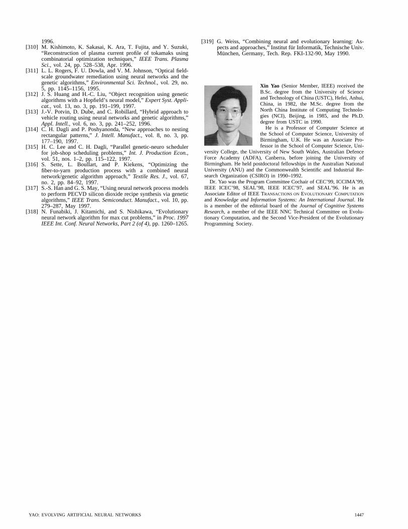
1996.[310] M. Kishimoto, K. Sakasai, K. Ara, T. Fujita, and Y. Suzuki,

“Reconstruction of plasma current profile of tokamaks usingcombinatorial optimization techniques,”IEEE Trans. PlasmaSci., vol. 24, pp. 528–538, Apr. 1996.

[311] L. L. Rogers, F. U. Dowla, and V. M. Johnson, “Optical field-scale groundwater remediation using neural networks and thegenetic algorithms,”Environmental Sci. Technol., vol. 29, no.5, pp. 1145–1156, 1995.

[312] J. S. Huang and H.-C. Liu, “Object recognition using geneticalgorithms with a Hopfield’s neural model,”Expert Syst. Appli-cat., vol. 13, no. 3, pp. 191–199, 1997.

[313] J.-V. Potvin, D. Dube, and C. Robillard, “Hybrid approach tovehicle routing using neural networks and genetic algorithms,”Appl. Intell., vol. 6, no. 3, pp. 241–252, 1996.

[314] C. H. Dagli and P. Poshyanonda, “New approaches to nestingrectangular patterns,”J. Intell. Manufact., vol. 8, no. 3, pp.177–190, 1997.

[315] H. C. Lee and C. H. Dagli, “Parallel genetic-neuro schedulerfor job-shop scheduling problems,”Int. J. Production Econ.,vol. 51, nos. 1–2, pp. 115–122, 1997.

[316] S. Sette, L. Boullart, and P. Kiekens, “Optimizing thefiber-to-yarn production process with a combined neuralnetwork/genetic algorithm approach,”Textile Res. J., vol. 67,no. 2, pp. 84–92, 1997.

[317] S.-S. Han and G. S. May, “Using neural network process modelsto perform PECVD silicon dioxide recipe synthesis via geneticalgorithms,” IEEE Trans. Semiconduct. Manufact., vol. 10, pp.279–287, May 1997.

[318] N. Funabiki, J. Kitamichi, and S. Nishikawa, “Evolutionaryneural network algorithm for max cut problems,” inProc. 1997IEEE Int. Conf. Neural Networks, Part 2 (of 4), pp. 1260–1265.

[319] G. Weiss, “Combining neural and evolutionary learning: As-pects and approaches,” Institut fur Informatik, Technische Univ.Munchen, Germany, Tech. Rep. FKI-132-90, May 1990.

Xin Yao (Senior Member, IEEE) received theB.Sc. degree from the University of Scienceand Technology of China (USTC), Hefei, Anhui,China, in 1982, the M.Sc. degree from theNorth China Institute of Computing Technolo-gies (NCI), Beijing, in 1985, and the Ph.D.degree from USTC in 1990.

He is a Professor of Computer Science atthe School of Computer Science, University ofBirmingham, U.K. He was an Associate Pro-fessor in the School of Computer Science, Uni-

versity College, the University of New South Wales, Australian DefenceForce Academy (ADFA), Canberra, before joining the University ofBirmingham. He held postdoctoral fellowships in the Australian NationalUniversity (ANU) and the Commonwealth Scientific and Industrial Re-search Organization (CSIRO) in 1990–1992.

Dr. Yao was the Program Committee Cochair of CEC’99, ICCIMA’99,IEEE ICEC’98, SEAL’98, IEEE ICEC’97, and SEAL’96. He is anAssociate Editor of IEEE TRANSACTIONS ON EVOLUTIONARY COMPUTATION

and Knowledge and Information Systems: An International Journal. Heis a member of the editorial board of theJournal of Cognitive SystemsResearch, a member of the IEEE NNC Technical Committee on Evolu-tionary Computation, and the Second Vice-President of the EvolutionaryProgramming Society.


evolving artiﬁcial neural networksxin/papers/published_iproc_sep99.pdf · evolving artiﬁcial...

Documents