ex ante efficiency implies incentive compatibility · ex ante efficiency implies incentive...
TRANSCRIPT

Economic Theory (2008) 36:35–55DOI 10.1007/s00199-007-0261-4
RESEARCH ARTICLE
Ex ante efficiency implies incentive compatibility
Yeneng Sun · Nicholas C. Yannelis
Received: 11 March 2007 / Revised: 3 May 2007 / Published online: 25 May 2007© Springer-Verlag 2007
Abstract We show that when agents become informationally negligible in a largeeconomy with asymmetric information, every ex ante efficient allocation must beincentive compatible. This means that any ex ante core or Walrasian allocation isincentive compatible. The corresponding result is false for fixed finite-agent economieswith asymmetric information. An example is also constructed to show that the ex postversion of the result does not hold. Furthermore, we show that the result is sharp inthe sense that it will fail to hold if one relaxes any of the main assumptions, namely,strong conditional independence on the information structure, strict concavity on theutility functions, type independence on the utility functions and endowments.
Keywords Asymmetric information · Pareto efficiency · Incentive compatibility ·Negligible private information · Strong conditional independence ·Exact law of large numbers
JEL Classification Numbers D0 · D5 · D6 · D8 · C0
Y. Sun (B)Department of Economics, National University of Singapore,1 Arts Link, Singapore 117570, Singaporee-mail: [email protected]
N. C. YannelisDepartment of Economics, University of Illinois at Urbana-Champaign,Champaign, IL 61820, USAe-mail: [email protected]
123

36 Y. Sun, N. C. Yannelis
1 Introduction
It is well known that in a finite-agent economy with asymmetric information, theremay not exist any incentive compatible, efficient allocations.1 However, intuition sug-gests that a perfectly competitive market should still perform efficiently since nosingle agent has monopoly power on information. This intuitive idea of perfect com-petition for an atomless economy with asymmetric information is formalized in Sunand Yannelis (2007). In particular, it is shown in Sun and Yannelis (2007) that thereexists an incentive compatible, ex post efficient allocation in a perfectly competitiveasymmetric information economy, and thus the well-known conflict between incentivecompatibility and Pareto efficiency is resolved exactly.2
While the existence of incentive compatible and ex post efficient allocations isshown in Sun and Yannelis (2007). It is easy to construct a large asymmetric informa-tion economy satisfying all the relevant conditions, and yet it has an ex post efficientallocation which is not incentive compatible (see Proposition 2 below). The purposeof this paper is to show that if we shift our attention to the ex ante case, then a totallydifferent type of result can be obtained. That is, every ex ante efficient allocation isincentive compatible (see Theorem 1 below). The result is shown under the assump-tions of strong conditional independence on the information structure, strict concavityon the utility functions, type independence on the utility functions and endowments.Such a result is obviously false in a fixed finite-agent economy with asymmetric in-formation, and there are no analogous results in the literature.
The proof of Theorem 1 requires four main assumptions, namely, strong conditionalindependence on the information structure, strict concavity on the utility functions,type independence on the utility functions and endowments. We show that if onerelaxes any of those assumptions, Theorem 1 may fail to hold. In particular, Propo-sition 3 shows that if the strong (conditional) independence is relaxed to a slightlyweaker condition of mutual independence, then there exists a large asymmetric infor-mation economy in which every allocation has an essentially equivalent version that isnot incentive compatible. Proposition 4 shows the importance of the strict concavitycondition on the utility functions while Propositions 5 and 6 demonstrate that Theorem1 cannot be extended to allow either initial endowments or utility functions to dependon private signals.
The paper is organized as follows. Sections 2 and 3 introduce, respectively theinformation structure and an economy with negligible asymmetric information. Themain result is presented in Sect. 4. The relationship between ex ante and ex postefficiency is studied in Sect. 5. In particular, it is shown that ex ante efficiency impliesex post efficiency while the latter does not imply incentive compatibility. Section 6shows that the main result may fail to hold if one relaxes any of the main assumptions.
1 See, for example (Glycopantis and Yannelis, 2005, p. vi, Example 0.1).2 Several other different approaches for related problems have also been proposed by different authors.Prescott and Townsend (1984) introduced a lottery model and showed the existence of incentive compatible,ex ante efficient lottery allocations. Based on a notion of informational smallness, McLean and Postlewaite(2002) showed the existence of incentive compatible, ex post efficient allocations in an approximate sensefor a replica economy. Hahn and Yannelis (1997) focused on a second best Pareto efficiency notion whichresults in incentive compatible allocations.
123

Ex ante efficiency implies incentive compatibility 37
All the proofs are given in the appendix. Finally, we note that our exact result inTheorem 1 on an atomless economy with asymmetric information have asymptoticanalogs for large but finite asymmetric information economies; this is illustrated inSect. 6 of Sun and Yannelis (2007).
2 The information structure
We fix an atomless probability space3 (I, I, λ) representing the space of economicagents, and S = s1, s2, . . . , sK the space of true states of nature (its power setdenoted by S), which are not known to the agents. Let T 0 = q1, q2, . . . , qL be thespace of all the possible signals (types) for individual agents, (T, T ) a measurablespace that models the private signal profiles for all the agents, and therefore T isa space of functions from I to T 0.4 Thus, t ∈ T , as a function from I to T 0, representsa private signal profile for all agents in I . For agent i ∈ I , t (i) (also denoted by ti ) isthe private signal of agent i while t−i the restriction of the signal profile t to the setI \ i of agents different from i ; let T−i be the set of all such t−i . For simplicity, weshall assume that (T, T ) has a product structure so that T is a product of T−i and T 0,while T is the product algebra of the power set T 0 on T 0 with a σ -algebra T−i onT−i . For t ∈ T and t ′i ∈ T 0, we shall adopt the usual notation (t−i , t ′i ) to denote thesignal profile whose value is t ′i for agent i , and the same as t for other agents.
Let (Ω,F , P) be a probability space representing all the uncertainty on the truestates as well as on the signals for all the agents, where (Ω,F) is the product measur-able space (S ×T,S ⊗T ). Let P S and PT be the marginal probability measures of P ,respectively on (S,S) and on (T, T ). Let s and ti , i ∈ I be the respective projectionmappings from Ω to S and from Ω to T 0 with ti (s, t) = ti .5 For each true state s ∈ S,we assume without loss of generality that the state is non-redundant in the sense thatπs = P S(s) > 0; let PT
s be the conditional probability measure on (T, T ) when therandom variable s takes value s. Thus, for each B ∈ T , PT
s (B) = P(s × B)/πs . Itis obvious that PT = ∑
s∈S πs PTs . Note that the conditional probability measure PT
sis often denoted as P(·|s) in the literature.
For i ∈ I , let τi be the signal distribution of agent i on the space T 0,6 andP S×T−i (·|ti ) the conditional probability measure on the product measurable space(S × T−i ,S ⊗ T−i ) when the signal of agent i is ti ∈ T 0. If τi (ti ) > 0, then it isclear that for D ∈ S ⊗ T−i , P S×T−i (D|ti ) = P(D × ti )/τi (ti ).
For s ∈ S, let PT−is and τis be the marginal probability measures of PT
s , respectivelyon (T−i , T−i ) and (T 0, T 0). Since redundant signals are allowed for agent i ∈ I(q ∈ T 0 is a redundant signal for agent i if τi (q) = 0), we shall impose the
3 We use the convention that all probability spaces are countably additive.4 In the literature, one usually assumes that different agents have possibly different sets of signals andrequire that the agents take all their own signals with positive probability. For notational simplicity, wechoose to work with a common set T 0 of signals, but allow zero probability for some of the redundantsignals. There is no loss of generality in this latter approach.5 ti can also be viewed as a projection from T to T 0.6 For q ∈ T 0, τi (q) is the probability P(ti = q).
123

38 Y. Sun, N. C. Yannelis
assumption that for any q ∈ T 0, if τi (q) > 0, then τis(q) > 0 for all s ∈ S,which means that any non-redundant signal has positive probability conditioned onany given true state.
Let F be the private signal process from I × T to T 0 such that F(i, t) = ti for any(i, t) ∈ I × T . In this paper, we need to work with F that is independent conditionedon the true states s ∈ S. However, an immediate technical difficulty arises, which isthe so-called measurability problem of independent processes. In our context, a signalprocess that is essentially independent, conditioned on the true states of nature is neverjointly measurable in the usual sense except for trivial cases.7 Hence, we need to workwith a joint agent-probability space (I × T, I T , λ PT
s ) that extends the usualmeasure-theoretic product (I ×T, I ⊗T , λ⊗ PT
s ) of the agent space (I, I, λ) and theprobability space (T, T , PT
s ), and retains the Fubini property.8 Its formal definitionis given in Definition 2 of the Appendix.
Let I F be the collection of all subsets A of I × Ω such that there are setsAs ∈ I T for s ∈ S such that A = ∪s∈S(i, s, t) ∈ I ×Ω : (i, t) ∈ As. By abusingthe notation, we can denote I F by (I T )⊗S. Define λ P on I F by lettingλ P(A) = ∑
s∈S πs(λ PTs )(As). Thus, one can view λ PT
s as the conditionalprobability measure on I × T , given s = s.
We shall assume that F is a measurable process from (I ×T, IT ) to T 0. When thetrue state is s, the signal distribution of agent i conditioned on the true state is PT
s F−1i ,
i.e., the probability for agent i to have q ∈ T 0 as her signal is PTs (F−1
i (q)), whereFi = F(i, ·). Let µs be the agents’ average signal distribution conditioned on thetrue state s, i.e.,
µs(q) =∫
I
PTs (F−1
i (q))dλ =∫
I
∫
T
1q(F(i, t))d PTs dλ, (1)
where 1q is the indicator function of the singleton set q. We shall impose thefollowing non-triviality assumption on the process F :
∀s, s′ ∈ S, s = s′ ⇒ µs = µs′ .
This says that different true states of nature correspond to different average conditionaldistributions of agents’ signals.
3 The large private information economy
We shall now follow the definition and notation in Sect. 2. We consider a large economywith asymmetric information. The space of agents is the atomless probability space(I, I, λ). In this economy, agents i ∈ I are informed with their private signals ti ∈ T 0
7 See Sun (2006) and Sun and Yannelis (2007), and their references for detailed discussion of the measur-ability problem.8 I T is a σ -algebra that contains the usual product σ -algebra I ⊗T , and the restriction of the countablyadditive probability measure λ PT
s to I ⊗ T is λ ⊗ PTs .
123

Ex ante efficiency implies incentive compatibility 39
but not the true state, and they can have contingent consumptions based on the signalprofiles t ∈ T announced by all the agents. Decisions are made at the ex ante level.The common consumption set is the positive orthant R
m+. In the sequel, we shall stateseveral assumptions on the economy.
A1. The utility function of each agent depends on her consumption x ∈ Rm+ and the
true state s ∈ S but not on the private signals of the agents in the economy.Thus, we can let u be a function from I ×R
m+ × S to R+ such that for any giveni ∈ I , u(i, x, s) is the utility of agent i at consumption bundle x ∈ R
m+ and truestate s ∈ S.
A2. For any given s ∈ S, u(i, x, s), (also denoted by us(i, x)),9 is I-measurable ini ∈ I , continuous, strictly concave and monotonic10 in x ∈ R
m+.A3. Let e be a λ-integrable function from I to R
m+ with e(i) as the initial endowmentof agent i .11
A4. The private signal process F is a measurable process from (I × T, I T ) toT 0 that is strongly conditionally independent, given s in the sense that forany i ∈ I , agent i’s signal F(i, ·) is independent of all the events in the signalspace (T−i , T−i ), conditioned on the true states of nature.12 In other words,for each s ∈ S, the probability space (T, T , PT
s ) is the product of its marginal
probability spaces (T−i , T−i , PT−is ) and (T 0, T 0, τis).
The Assumption A4 says that conditioned on the true states of nature, the privatesignal of an individual agent has strictly no influence over any others. Thus, perfectcompetition prevails in this economy in the sense that agents have negligible initialendowments and negligible private information.
We shall now consider an economy where the agents are informed with their signalsbut not the true state. Formally, the collection E p = (I ×Ω, IF , λ P), u, e, F, sis called a private information economy.
The space of consumption plans for the economy E p is the space L1(PT , Rm+) of
integrable functions from (T, T , PT ) to Rm+, which is infinite dimensional. Fix an
agent i ∈ I . For a consumption plan z ∈ L1(PT , Rm+), let
U pi (z) =
∫
Ω
u(i, z(t), s)d P (2)
be the ex ante expected utility of agent i for the consumption plan z.13
9 In the sequel, we shall often use subscripts to denote some variable of a function that is viewed as aparameter in a particular context.10 The utility function u(i, ·, s) is monotonic if for any x, y ∈ R
m+ with x ≤ y and x = y, u(i, x, s) <
u(i, y, s).11 Since the true state s ∈ S is not known to the agents, the agents’ endowments cannot depend on s.However, as in McLean and Postlewaite (2002) and Sun and Yannelis (2007), here we also assume that theendowments do not depend on the private signals of agents.12 For a general justification of using conditional independence, see Hammond and Sun (2003).13 Fix i ∈ I . Since u(i, ·, s) is strictly concave for each s ∈ S, there are constants c, d ∈ R+ such thatu(i, x, s) ≤ c‖x‖ + d for any x ∈ R
m+, where ‖ · ‖ is the Euclidean norm. From this condition, it is clearthat
∫Ω u(i, z(t), s)d P is finite.
123

40 Y. Sun, N. C. Yannelis
Definition 1 1. An allocation for the economy E p is an integrable function x p from(I ×T, I T , λ PT ) to R
m+; agent i’s consumption plan is x p(i, ·) (also denotedby x p
i ).2. An allocation x p is feasible if for PT -almost all t ∈ T ,
∫I x p(i, t)dλ(i) =∫
I e(i)dλ(i).3. A feasible allocation x p is said to be ex ante efficient if there does not exist a
feasible allocation y p such that for λ-almost all i ∈ I , U pi (y p
i ) > U pi (x p
i ).4. A feasible allocation x p is said to be ex post efficient if for PT -almost all t ∈ T , x p
tis efficient in the large deterministic (ex post) economyE p
t =(I, I, λ),U (·, ·, t), e,where U (i, x, t) = ∑
s∈S ui (x, s)P S(s|t) is the ex post utility of agent i (alsodenoted by Ui (x |t)) for her consumption bundle x ∈ R
m+ with the given signalprofile t .
5. For an allocation x p, an agent i ∈ I , private signals ti , t ′i ∈ T 0, let
Ui (x pi , t ′i |ti ) =
∫
S×T−i
ui (x pi (t−i , t ′i ), s)d P S×T−i (·|ti ), (3)
be the interim expected utility of agent i when she receives private signal ti butmis-reports as t ′i . The allocation x p is said to be incentive compatible if λ-almostall i ∈ I ,
Ui (x pi , ti |ti ) ≥ Ui (x p
i , t ′i |ti )
holds for all the non-redundant signals ti , t ′i ∈ T 0 of agent i (i.e., τi (ti ) > 0 andτi (t ′i ) > 0).
6. A feasible allocation x p is said to be an ex ante Walrasian allocation (ex antecompetitive equilibrium allocation) if there is a bounded measurable price functionp from (T, T ) to R
m+ \ 0 such that for λ-almost all i ∈ I , x p(i) is a maximalelement in the budget set
⎧⎨
⎩z ∈ L1(PT , R
m+) :∫
T
p(t) · z(t)d PT ≤∫
T
p(t) · e(i)d PT
=⎛
⎝∫
T
p(t)d PT
⎞
⎠ · e(i)
⎫⎬
⎭
under the expected utility function U pi (·).
7. A coalition A (i.e., a set in I with λ(A) > 0) is said to ex ante block an allocationx p in E p if there exists an allocation y p such that
∫A y p(i, t)dλ(i) = ∫
A e(i)dλ(i)for PT -almost all t ∈ T , and for λ-almost all i ∈ A, U p
i (y pi )) > U p
i (x pi ).14
14 One can also only define the allocation y p on A × T instead of I × T . However, there is no loss ofgenerality since one can always extend a function defined on A × T to I × T to keep its integrability.
123

Ex ante efficiency implies incentive compatibility 41
A feasible allocation x p is said to be in the ex ante core of E p, or simply an exante core allocation in E p, if there is no coalition that ex ante blocks x p.
4 The main theorem
We are now ready to state the main result of this paper. Its proof will be given inSubsect. 7.2 of the appendix.
Theorem 1 Under Assumptions A1–A4, any ex ante efficient allocation is incentivecompatible.
It is obvious that any ex ante core allocation is ex ante efficient. It is also easy tocheck that any ex ante Walrasian allocation is ex ante efficient. Hence the followingtwo corollaries are clear consequences of Theorem 1.
Corollary 1 Under Assumptions A1–A4, any ex ante core allocation is incentivecompatible.
Corollary 2 Under Assumptions A1–A4, any ex ante Walrasian allocation is incen-tive compatible.
5 Ex ante versus ex post efficiency
In this section, we adopt the economic model specified in Sects. 2 and 3. We assumethat Assumptions A1–A4 are satisfied.
As noted in Holmström and Myerson (1983), ex ante efficiency implies expost efficiency for a finite-agent economy. The ex post efficiency in Holmström andMyerson (1983) requires all the states to be revealed, and thus incentive compatibilityis not an issue. In contrast, the notion of ex post efficiency as considered in McLeanand Postlewaite (2002) for a countable replica economy and Sun and Yannelis (2007)for an atomless private information economy requires only the signals to be revealedbut not the true states. Nevertheless, the following proposition, whose proof will begiven in Subsect. 7.3 of the appendix, shows that ex ante efficiency does imply ex postefficiency in our setting.
Proposition 1 Every ex ante efficient allocation is ex post efficient.
Theorem 1 above shows that incentive compatibility follows form ex ante effi-ciency. However, this is not the case for ex post efficiency. In particular, the followingproposition shows that there exists an ex post efficient allocation that is not incentivecompatible;15 by Theorem 1, such an allocation is not ex ante efficient. This meansthat the converse of Proposition 1 is not true.
Proposition 2 There exists a large private information economy such that (1) it sat-isfies all the conditions on the information structure in Sect. 2 as well as AssumptionsA1–A4 in Sect. 3; (2) it has an ex post efficient allocation that is not incentive com-patible.
15 The details of the construction can be found in Subsect. 7.4 of the appendix.
123
42 Y. Sun, N. C. Yannelis
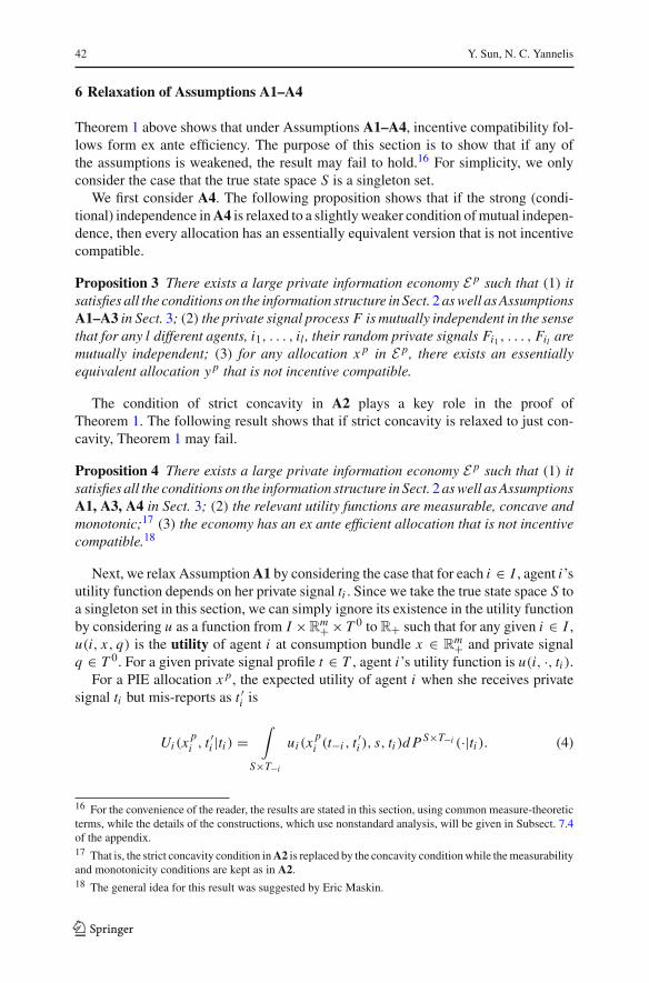
6 Relaxation of Assumptions A1–A4
Theorem 1 above shows that under Assumptions A1–A4, incentive compatibility fol-lows form ex ante efficiency. The purpose of this section is to show that if any ofthe assumptions is weakened, the result may fail to hold.16 For simplicity, we onlyconsider the case that the true state space S is a singleton set.
We first consider A4. The following proposition shows that if the strong (condi-tional) independence in A4 is relaxed to a slightly weaker condition of mutual indepen-dence, then every allocation has an essentially equivalent version that is not incentivecompatible.
Proposition 3 There exists a large private information economy E p such that (1) itsatisfies all the conditions on the information structure in Sect. 2 as well as AssumptionsA1–A3 in Sect. 3; (2) the private signal process F is mutually independent in the sensethat for any l different agents, i1, . . . , il , their random private signals Fi1, . . . , Fil aremutually independent; (3) for any allocation x p in E p, there exists an essentiallyequivalent allocation y p that is not incentive compatible.
The condition of strict concavity in A2 plays a key role in the proof ofTheorem 1. The following result shows that if strict concavity is relaxed to just con-cavity, Theorem 1 may fail.
Proposition 4 There exists a large private information economy E p such that (1) itsatisfies all the conditions on the information structure in Sect. 2 as well as AssumptionsA1, A3, A4 in Sect. 3; (2) the relevant utility functions are measurable, concave andmonotonic;17 (3) the economy has an ex ante efficient allocation that is not incentivecompatible.18
Next, we relax Assumption A1 by considering the case that for each i ∈ I , agent i’sutility function depends on her private signal ti . Since we take the true state space S toa singleton set in this section, we can simply ignore its existence in the utility functionby considering u as a function from I ×R
m+ × T 0 to R+ such that for any given i ∈ I ,u(i, x, q) is the utility of agent i at consumption bundle x ∈ R
m+ and private signalq ∈ T 0. For a given private signal profile t ∈ T , agent i’s utility function is u(i, ·, ti ).
For a PIE allocation x p, the expected utility of agent i when she receives privatesignal ti but mis-reports as t ′i is
Ui (x pi , t ′i |ti ) =
∫
S×T−i
ui (x pi (t−i , t ′i ), s, ti )d P S×T−i (·|ti ). (4)
16 For the convenience of the reader, the results are stated in this section, using common measure-theoreticterms, while the details of the constructions, which use nonstandard analysis, will be given in Subsect. 7.4of the appendix.17 That is, the strict concavity condition in A2 is replaced by the concavity condition while the measurabilityand monotonicity conditions are kept as in A2.18 The general idea for this result was suggested by Eric Maskin.
123

Ex ante efficiency implies incentive compatibility 43
The incentive compatibility can be defined in the same way as in Definition 1. For aconsumption plan z ∈ L1(PT , R
m+), the ex ante utility can be defined as in equation(2) by
U pi (z) =
∫
Ω
u(i, z(t), s, ti )d P (5)
Proposition 5 below shows that if Assumption A1 is relaxed to allow type dependentutilities, then Theorem 1 can fail strongly so that every ex ante efficient allocationin some large private information economy is not incentive compatible. On the otherhand, the economy in Proposition 5 does have an incentive compatible, ex post efficientallocation as shown by Theorem 2 of Sun and Yannelis (2007).
Proposition 5 There exists a large private information economy E p such that (1) itsatisfies all the conditions on the information structure in Sect. 2 as well as AssumptionsA2–A4 in Sect. 3; (2) agent i’s utility function depends on her private signal ti asdescribed above; (3) every ex ante efficient allocation in the economy is not incentivecompatible.
Finally, we relax Assumption A3 by considering the case that for each i ∈ I , agenti’s endowment depends on her private signals. Let e be a function from I × T 0 to R
m+with e(i, ti ) as the initial endowment of agent i with private signal ti . We assume thatfor each q ∈ T 0, e(i, q) is λ-integrable.
Fix an allocation x p. When agents’ endowments do not depend on their privatesignals, Eq. (3) defines the expected utility of agent i when she receives private signalti but mis-reports as t ′i . If we consider the case that the endowment of every agentdepends on her private signal as above, then the expected utility of agent i when shereceives private signal ti but mis-reports as t ′i is19
Ui (x pi , t ′i |ti ) =
∫
S×T−i
ui (x pi (t−i , t ′i ) − e(t ′i ) + e(ti ), s)d P S×T−i (·|ti ). (6)
The incentive compatibility can be defined in the same way as in Definition 1.
Proposition 6 There exists a large private information economy E p such that (1) itsatisfies all the conditions on the information structure in Sect. 2 as well as AssumptionsA1, A2, A4 in Sect. 3; (2) agent i’s endowment depends on her private signal ti asdescribed above; (3) every ex ante efficient allocation in the economy is not incentivecompatible.
19 The idea is that when agent i receives private signal ti but mis-reports as t ′i , her total consumption is her
endowment e(ti ) plus her net trade x pi (t−i , t ′i ) − e(t ′i ).
123

44 Y. Sun, N. C. Yannelis
7 Appendix
7.1 The exact law of large numbers
In order to work with independent processes constructed from signal profiles, we needto work with an extension of the usual measure-theoretic product that retains the Fubiniproperty. Below is a formal definition of the Fubini extension in Definition 2.2 of Sun(2006).
Definition 2 A probability space (I × Ω,W, Q) extending the usual product space(I × Ω, I ⊗ F , λ ⊗ P) is said to be a Fubini extension of (I × Ω, I ⊗ F , λ ⊗ P) iffor any real-valued Q-integrable function f on (I × Ω,W),
(1) the two functions fi and fω are integrable, respectively on (Ω,F , P) forλ-almost all i ∈ I , and on (I, I, λ) for P-almost all ω ∈ Ω;
(2)∫Ω
fi d P and∫
I fωd P are integrable, respectively on (I, I, λ) and (Ω,F , P),with
∫I×Ω
f d Q = ∫I
(∫Ω
fi d P)
dλ = ∫Ω
(∫I fωdλ
)d P .20
To reflect the fact that the probability space (I × Ω,W, Q) has (I, I, λ) and(Ω,F , P) as its marginal spaces, as required by the Fubini property, it will be denotedby (I × Ω, I F , λ P).
We shall now follow the notation of Sect. 2. When the probability space (I ×T, I T , λ PT
s ) is a Fubini extension of the usual product space (I ×T, I⊗T , λ⊗ PTs ), for
each s ∈ S, it can be checked that (I ×Ω, I F , λ P), defined in the last paragraphof Sect. 2, is a Fubini extension of the usual product space (I × Ω, I ⊗ F , λ ⊗ P).
The following is an exact law of large numbers for a continuum of independentrandom variables shown in Sun (2006), which is stated here as a lemma using ournotation for the convenience of the reader.21
Lemma 1 If a I T -measurable process G from I × T to a complete separablemetric space X is essentially pairwise independent conditioned on s in the sensethat for λ-almost all i ∈ I , the random variables Gi and G j from (T, T , PT
s ) toX are independent for λ-almost all j ∈ I , then for each s ∈ S, the cross-sectionaldistribution λG−1
t of the sample function Gt (·) = G(t, ·) is the same as the distribution(λ PT
s )G−1 of the process G viewed as a random variable on (I ×T, IT , λ PTs )
for PTs -almost all t ∈ T . In addition, for each s ∈ S, when X is the real line R and G
is (λ PTs )-integrable,
∫I Gt dλ = ∫
I×T Gd(λ PTs ) holds for PT
s -almost all t ∈ T .
7.2 Proof of Theorem 1
Let x p be any ex ante efficient allocation. Then the Fubini property implies that thereis a set A∗ ∈ I with λ(A∗) = 1 such that for any i ∈ A∗ and any s ∈ S, the integral
20 The classical Fubini Theorem is only stated for the usual product measure spaces. It does not apply tointegrable functions on (I × Ω, W, Q) since these functions may not be I ⊗ F -measurable. However,the conclusions of that theorem do hold for processes on the enriched product space (I × Ω, W, Q) thatextends the usual product.21 See Corollaries 2.9 and 2.10 in Sun (2006). We state the result using a complete separable metric spaceX for the sake of generality. In particular, a finite space or an Euclidean space is a complete separable metricspace.
123

Ex ante efficiency implies incentive compatibility 45
∫T x p(i, t)d PT
s is finite.22 We can define an allocation x p by letting x pi (·) = x p
i (·)for i ∈ A∗ and x p
i (·) ≡ ei for i /∈ A∗. Then, the integral∫
T x p(i, t)d PTs is finite for
all i ∈ I and s ∈ S. It is obvious that x p is feasible and ex ante efficient.Define the following sets
∀s ∈ S, Ls = t ∈ T : λF−1t = µs; L0 = T − ∪s∈S Ls .
The non-triviality assumption implies that for any s, s′ ∈ S with s = s′, Ls ∩ Ls′ = ∅.The measurability of the sets Ls, s ∈ S and L0 follows from the measurability of F .Thus, the collection L0 ∪ Ls, s ∈ S forms a measurable partition of T .
By Eq. (1) and the Fubini property for (I × T, I T , λ PTs ), we have µs(q) =∫
I×T 1q(F(i, t))d(λ PTs ) for any q ∈ T 0. Thus, µs is actually the distribution
(λ PTs )F−1 of F , viewed as a random variable on the product space I × T . Since
the signal process F satisfies the condition of conditional independence, it certainlysatisfies the condition of essential pairwise conditional independence, the exact lawof large numbers in Lemma 1 implies that PT
s (Ls) = 1 for each s ∈ S.For each (i, t) ∈ I × T , let
y p(i, t) =⎧⎨
⎩
∫
Ie(i)dλ if t ∈ L0,
∫
Tx p(i, t ′)d PT
s (t ′) if t ∈ Ls, s ∈ S.(7)
Since the Fubini property implies that∫
T x p(·, t)d PTs (t) is I-measurable on I , it is
clear that y p is I ⊗ T -measurable and hence I T -measurable. For t ∈ L0, y p(·, t)is the constant
∫I e(i)dλ and thus
∫I y p(i, t)dλ = ∫
I e(i)dλ; for s ∈ S and t ∈ Ls ,y p(i, t) is
∫T x p(i, t)d PT
s , and hence
∫
I
y p(i, t)dλ(i) =∫
I
∫
T
x p(i, t ′)d PTs (t ′)dλ(i)
=∫
T
∫
I
x p(i, t ′)dλ(i)d PTs (t ′) =
∫
I
e(i)dλ(i),
where the last identity follows from the feasibility of x p. Therefore, y p is a feasibleallocation in E p that satisfies the feasibility condition for all t ∈ T .
We shall prove that x p(i, t) = y p(i, t) for λ PT -almost all (i, t) ∈ I × T .Suppose not; then there exist s0 ∈ S and coalition A ∈ I (with λ(A) > 0) such thatfor each i ∈ A, PT
s0(t ∈ T : x p(i, t) = y p(i, t)) > 0, i.e., the random variable x p
i (·)is not essentially constant under the probability measure PT
s0. For each i ∈ A, since
22 The Fubini property only implies the integrability of x p(i, ·) for λ-almost i ∈ I . It also means thatx p(i, ·) may not be integrable for i in a λ-null subset of I .
123

46 Y. Sun, N. C. Yannelis
u(i, ·, s0) is strictly concave, Jensen’s inequality implies that
∫
T
ui (x pi (t), s0)d PT
s0(t) < ui
⎛
⎝∫
T
x pi (t)d PT
s0, s0
⎞
⎠ . (8)
The assumption of monotonicity implies that for each i ∈ A, ui (0, s0) ≤ ui (x pi (t), s0)
for all t ∈ T , which implies that ui (0, s0) ≤ ∫T ui (x p
i (t), s0)d PTs0
(t). By Eq. (8), wehave for each i ∈ A, ui (0, s0) < ui
(∫T x p
i (t)d PTs0
, s0), and hence
∫T x p
i (t)d PTs0
musthave positive components. By the continuity of the utility functions u(i, ·, s0), one canchoose a coalition A0 ⊆ A (with 0 < λ(A0) < 1), a positive number ε0 and a vectore0 ∈ R
m+ with e0 = 0 such that for any i ∈ A0,∫
T x pi (t)d PT
s0≥ e0, and
∫
T
ui (x pi (t), s0)d PT
s0(t) + ε0 < ui
⎛
⎝∫
T
x pi (t)d PT
s0, s0
⎞
⎠
< ui
⎛
⎝∫
T
x pi (t)d PT
s0− e0, s0
⎞
⎠ + ε0. (9)
For each (i, t) ∈ I × T , let
z p(i, t) =⎧⎨
⎩
y p(i, t) for (i, t) ∈ I × (T \ Ls0),
y p(i, t) − e0 for (i, t) ∈ A0 × Ls0 ,
y p(i, t) + λ(A0)1−λ(A0)
e0 for (i, t) ∈ (I \ A0) × Ls0 .
(10)
It is obvious that z p is I T -measurable. When (i, t) ∈ A0 × Ls0 , z p(i, t) =y p(i, t) − e0 = ∫
T x pi (t ′)d PT
s0(t ′) − e0 ≥ 0. It is thus clear that z p takes values
in Rm+. The feasibility of y p for all t ∈ T implies immediately that for t ∈ (T \ Ls0),∫
I z p(i, t)dλ = ∫I e(i)dλ. For t ∈ Ls0 ,
∫
I
z p(i, t)dλ =∫
A0
(y p(i, t) − e0)dλ +∫
I\A0
(
y p(i, t) + λ(A0)
1 − λ(A0)e0
)
dλ
=∫
I
y p(i, t)dλ − λ(A0)e0 + λ(I \ A0)λ(A0)
1 − λ(A0)e0
=∫
I
y p(i, t)dλ =∫
I
e(i)dλ.
Therefore, z p is a feasible allocation.
123
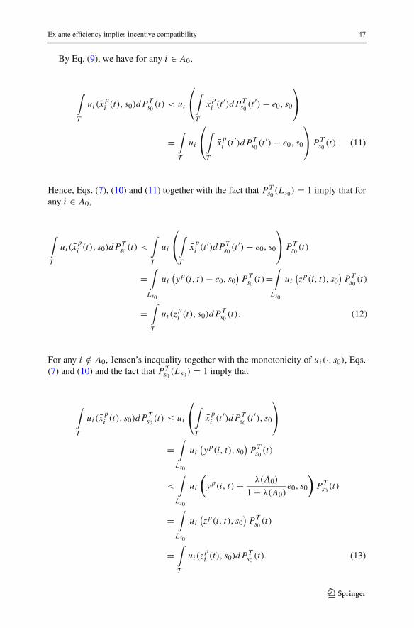
Ex ante efficiency implies incentive compatibility 47
By Eq. (9), we have for any i ∈ A0,
∫
T
ui (x pi (t), s0)d PT
s0(t) < ui
⎛
⎝∫
T
x pi (t ′)d PT
s0(t ′) − e0, s0
⎞
⎠
=∫
T
ui
⎛
⎝∫
T
x pi (t ′)d PT
s0(t ′) − e0, s0
⎞
⎠ PTs0
(t). (11)
Hence, Eqs. (7), (10) and (11) together with the fact that PTs0
(Ls0) = 1 imply that forany i ∈ A0,
∫
T
ui (x pi (t), s0)d PT
s0(t) <
∫
T
ui
⎛
⎝∫
T
x pi (t ′)d PT
s0(t ′) − e0, s0
⎞
⎠ PTs0
(t)
=∫
Ls0
ui(y p(i, t) − e0, s0
)PT
s0(t)=
∫
Ls0
ui(z p(i, t), s0
)PT
s0(t)
=∫
T
ui (zpi (t), s0)d PT
s0(t). (12)
For any i /∈ A0, Jensen’s inequality together with the monotonicity of ui (·, s0), Eqs.(7) and (10) and the fact that PT
s0(Ls0) = 1 imply that
∫
T
ui (x pi (t), s0)d PT
s0(t) ≤ ui
⎛
⎝∫
T
x pi (t ′)d PT
s0(t ′), s0
⎞
⎠
=∫
Ls0
ui(y p(i, t), s0
)PT
s0(t)
<
∫
Ls0
ui
(
y p(i, t) + λ(A0)
1 − λ(A0)e0, s0
)
PTs0
(t)
=∫
Ls0
ui(z p(i, t), s0
)PT
s0(t)
=∫
T
ui (zpi (t), s0)d PT
s0(t). (13)
123
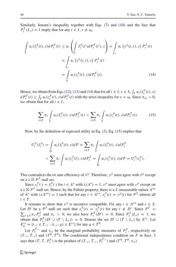
48 Y. Sun, N. C. Yannelis
Similarly, Jensen’s inequality together with Eqs. (7) and (10) and the fact thatPT
s (Ls) = 1 imply that for any i ∈ I , s = s0,
∫
T
ui (x pi (t), s)d PT
s (t) ≤ ui
⎛
⎝∫
T
x pi (t ′)d PT
s (t ′), s
⎞
⎠ =∫
Ls
ui(y p(i, t), s
)PT
s (t)
=∫
Ls
ui(z p(i, t), s
)PT
s (t)
=∫
T
ui (zpi (t), s)d PT
s (t). (14)
Hence, we obtain from Eqs. (12), (13) and (14) that for all i ∈ I , s ∈ S,∫
T ui (x pi (t), s)
d PTs (t) ≤ ∫
T ui (zpi (t), s)d PT
s (t) with the strict inequality for s = s0. Since πs0 > 0,we obtain that for all i ∈ I ,
∑
s∈S
πs
∫
T
ui (x pi (t), s)d PT
s (t) <∑
s∈S
πs
∫
T
ui (zpi (t), s)d PT
s (t). (15)
Now, by the definition of expected utility in Eq. (2), Eq. (15) implies that
U pi (x p
i ) =∫
Ω
ui (x pi (t), s)d P =
∑
s∈S
πs
∫
T
ui (x pi (t), s)d PT
s
<∑
s∈S
πs
∫
T
ui (zpi (t), s)d PT
s =∫
Ω
ui (zpi (t), s)d P = U p
i (z pi ).
This contradicts the ex ante efficiency of x p. Therefore, y p must agree with x p excepton a λ PT -null set.
Since x pi (·) = x p
i (·) for i ∈ A∗ with λ(A∗) = 1, x p must agree with y p except ona λ PT -null set. Hence, by the Fubini property, there is a I-measurable subset A∗∗of A∗ with λ(A∗∗) = 1 such that for any i ∈ A∗∗, x p
i (t) = y p(t) for PT -almost allt ∈ T .
It remains to show that x p is incentive compatible. Fix any i ∈ A∗∗ and s ∈ S.Let Di be a PT -null set such that x p
i (t) = y pi (t) for any t /∈ Di . Since PT =
∑s′∈S πs′ PT
s′ and πs > 0, we also have PTs (Di ) = 0. Since PT
s (Ls) = 1, weobtain that PT
s (Di ∪ (T \ Ls)) = 0. Denote the set Di ∪ (T \ Ls) by Eis . LetEis
q = t−i ∈ T−i : (t−i , q) ∈ Eis for any q ∈ T 0.
Let PT−is and τis be the marginal probability measures of PT
s , respectively on(T−i , T−i ) and (T 0, T 0). The conditional independence condition on F in Sect. 3says that (T, T , PT
s ) is the product of (T−i , T−i , PT−is ) and (T 0, T 0, τis).
123

Ex ante efficiency implies incentive compatibility 49
For any fixed ti , t ′i ∈ T 0 with τi (ti ) > 0 and τi (t ′i ) > 0, our assumption onnon-redundant signals in Sect. 2 implies that τis(ti ) > 0 and τis(t ′i ) > 0. Since
PTs (Eis) = PT
s (∪q∈T 0 Eisq × q) =
∑
q∈T 0
PT−is (Eis
q ) · τis(q) = 0,
we have PT−is (Eis
ti ) = PT−is (Eis
t ′i) = 0. Therefore, PT−i
s (Eisti ∪ Eis
t ′i) = 0.
For any fixed t−i /∈ Eisti ∪ Eis
t ′i, we have (t−i , ti ) /∈ Eis and (t−i , t ′i ) /∈ Eis , which
means that (t−i , ti ) ∈ Ls \ Di and (t−i , t ′i ) ∈ Ls \ Di . Since (t−i , ti ), (t−i , t ′i ) /∈ Di ,the property of the set Di implies that
x pi (t−i , ti ) = y p
i (t−i , ti ), and x pi (t−i , t ′i ) = y p
i (t−i , t ′i ). (16)
Since (t−i , ti ), (t−i , t ′i ) ∈ Ls , the definition of y p implies that
y pi (t−i , ti ) = y p
i (t−i , t ′i ) =∫
t ′′∈T
x p(i, t ′′)d PTs (t ′′), (17)
which also equals∫
t ′′∈T x p(i, t ′′)d PTs (t ′′) (since i also belongs to A∗). Hence, for any
t−i /∈ Eisti ∪ Eis
t ′i, Eqs. (16) and (17) imply that x p
i (t−i , ti ) = x pi (t−i , t ′i ).
The above identity and the fact that Eisti ∪ Eis
t ′iis a PT−i
s -null set imply that
∫
T−i
ui (x pi (t−i , ti ), s)PT−i
s =∫
T−i
ui (x pi (t−i , t ′i ), s)PT−i
s . (18)
It is easy to see that for any q ∈ T 0,
∫
S×T−i
ui (x pi (t−i , q), s)d P S×T−i (·|ti )
=∑
s∈S
πsτis(ti )τi (ti )
∫
T−i
ui (x pi (t−i , q), s)PT−i
s . (19)
By taking q to be ti or t ′i in Eq. (19), Eqs. (3) and (18) then imply that Ui (x pi , ti |ti ) =
Ui (x pi , t ′i |ti ). Therefore, the condition of incentive compatibility is satisfied by an
arbitrary ex ante efficient allocation x p.
7.3 Proof of Proposition 1
Let x p be an ex ante efficient allocation. We follow the proof of Theorem 1 to showthat x p and y p differ only on a λ PT -null set, where y p is defined in Eq. (7).
123

50 Y. Sun, N. C. Yannelis
Suppose that x p is not ex post efficient. Since x p and y p differ only on a λPT -nullset, the Fubini property implies that for PT -almost all t ∈ T , x p
t and y pt differ only
on a λ-null set. Thus, y p is ex ante efficient, but not ex post efficient.Let C be the set of t ∈ T such that y p
t is not efficient in the ex post large deterministiceconomy E p
t = (I, I, λ), U (·, ·, t), e. Then, C is not a null set under the measurePT , which also means that there exists s0 ∈ S such that C is not a null set under themeasure PT
s0.
As shown in the proof of Theorem 1 in Sun and Yannelis (2007), we have forPT -almost all t ∈ Ls0 , U (i, ·, t) = ∑
s∈S u(i, ·, s)P S(s|t) = u(i, ·, s0) for alli ∈ I . Hence, there is t0 ∈ C ∩ Ls0 such that U (·, ·, t0) = u(·, ·, s0). Thus, y p
t0 isnot efficient in the large deterministic economy E p
t0 = (I, I, λ), u(·, ·, s0), e, whichmeans that there exists a feasible allocation α for E p
t0 such that for λ-almost all i ∈ I ,
ui (α(i), s0) > ui (y pt0(i), s0) = ui (y p
t (i), s0) (20)
for all t ∈ Ls0 .Define a feasible allocation β p such that
β p(i, t) =
y p(i, t) if t ∈ Ls0 ,
α(i) if t ∈ Ls0 .(21)
Then, it is easy to see that U pi (β
pi ) > U p
i (y pi ) for λ-almost all i ∈ I , which contradicts
the ex ante efficiency of y p. Therefore, x p must be ex post efficient.
7.4 Proof of Propositions 2–6
In all the constructions of this subsection, we take S to be a singleton set. Thus, we canidentify Ω with T and P with PT . The constructions will use nonstandard analysis.One can pick up some background knowledge on nonstandard analysis from the firstthree chapters of the book Loeb and Wolff (2000).
We shall fix some notations first for this subsection. Fix n ∈ ∗N∞. Let
I = 1, 2, . . . , n with its internal power set I0 and internal counting probabilitymeasure λ0 on I0 with λ0(A) = |A|/|I | for any A ∈ I0, where |A| is the internalcardinality of A. Let (I, I, λ) be the Loeb space of the internal probability space(I, I0, λ0), which will serve as the space of agents for the large private informationeconomies considered in various constructions below.
Let T 0 = 0, 1 be the signals for individual agents, and T the set of all the internalfunctions from I to T 0 (the space of signal profiles). Let T0 be the internal power seton T , P0 an internal probability measure on (T, T0), and (T, T , P) the correspondingLoeb space. Except in the proof of Proposition 3 below, P0 will be taken to be theinternal counting probability measure on T0 in this subsection, i.e., the probabilityweight for each t = (t1, t2, . . . , tn) ∈ T under P0 is 1/2n ; and in this case it is obviousthat condition (A4) is satisfied.
Let (I ×T, I0 ⊗T0, λ0 ⊗ P0) be the internal product probability space of (I, I0, λ0)
and (T, T0, P0). Let (I × T, I T , λ P) be the Loeb space of the internal product
123

Ex ante efficiency implies incentive compatibility 51
(I × T, I0 ⊗ T0, λ0 ⊗ P0), which is indeed a Fubini extension of the usual productprobability space by Keisler’s Fubini Theorem (see, for example Loeb and Wolff(2000)).
Proof of Proposition 2: We consider a one-good economy with strictly concave andmonotonic utility functions ui : R+ → R+ and constant endowments ei = 1 for allthe agents i ∈ I . Thus, condition (1) of Proposition 2 is satisfied. Note that any feasibleallocation xi ≥ 0, i ∈ I (i.e.,
∫I xi dλ = 1) is efficient in the relevant deterministic
economy (I, I, λ), (ui , ei )i∈I .Next, define an allocation x p(i, t) = 2ti in the private information economy. Since
Assumption (A4) is satisfied, one can apply Lemma 1 to claim that for P-almost allt ∈ T ,
∫I x p
t (i)dλ = ∫I
∫T 2ti d Pdλ = 1, which means that x p is feasible and ex post
efficient. It is easy to see that
Ui (x pi , 1|0) =
∫
T−i
ui (x pi (t−i , 1))d PT−i = ui (2)
> ui (0) =∫
T−i
ui (x pi (t−i , 0))d PT−i = Ui (x p
i , 0|0). (22)
Hence, x p is not incentive compatible.
Proof of Proposition 3: We need to work with an internal probability measure P0 sothat Assumption (A4) is violated. Define an internal probability measure P0 on (T, T0)
such that for any t = (t1, t2, . . . , tn) ∈ T , its probability weight is defined by23
P0(t) = 1
2n−1 if∑n
j=1 t j is odd,0 if
∑nj=1 t j is even.
(23)
Fix any different agents i1, . . . , i ∈ I . For any k1, . . . , k ∈ 0, 1, if∑
j=1 k j
is odd, then
P0(t ∈ T : ti1 = k1, . . . , ti = k
)
= P0
⎛
⎝t ∈ T :∑
i =i1,...,i
ti is even, and ti1 = k1, . . . , ti = k
⎞
⎠
= 2n−−1 · 1
2n−1 = 1
2;
similarly, if∑
j=1 k j is even, one can also obtain that P0(t ∈ T : ti1 = k1, . . . , ti =k) = 1
2 . Hence, the random private signals Fi1 , . . . , Fi are mutually independent,which means that the private signal process F is mutually independent.
23 This definition is motivated by a classical example of Bernstein in Feller (1968, p. 126) and its general-ization in Wang (1979).
123

52 Y. Sun, N. C. Yannelis
Define a set A in T by letting A = t ∈ T : ∑nj=1 t j is odd.; then P(A) = 1.
Let e be the vector (1, . . . , 1) in Rm+. For i ∈ I , let ui and ei be the utility function
and endowment of agent i that satisfy Assumptions (A1)–(A3). For any allocationx p in the private information economy, define another allocation y p in the privateinformation economy such that for any (i, t) ∈ I × T ,
y p(i, t) =
x p(i, t) if t ∈ A,x p(i, t−i , 1 − ti ) + e if t ∈ A.
(24)
It is clear that y p is essentially equivalent to x p.For any fixed agent i ∈ I , let A−i = t−i ∈ T−i : ∑
j =i t j is odd.. Then it is
easy to see that PT−i (A−i |ti = 0) = 1 and PT−i (A−i |ti = 1) = 0, which meansthat Assumption (A4) is not satisfied. By equation (3) in the definition of incentivecompatibility,
Ui (y pi , t ′i |ti ) =
∫
S×T−i
ui (y pi (t−i , t ′i ))d PT−i (·|ti ),
and the monotonicity of the utility function ui , we can obtain that
Ui (y pi , 1|0) =
∫
A−i
ui (y pi (t−i , 1))d PT−i (·|ti = 0)
=∫
A−i
ui (x pi (t−i , 0) + e)d PT−i (·|ti = 0)
>
∫
A−i
ui (x pi (t−i , 0))d PT−i (·|ti = 0)
=∫
A−i
ui (y pi (t−i , 0))d PT−i (·|ti = 0) = Ui (y p
i , 0|0), (25)
which means that the allocation y p is not incentive compatible.
Proof of Proposition 4: We consider a one-good economy with utility functionsui (x) = x and constant endowments ei = 1 for all the agents i ∈ I . (1) and (2)of Proposition 4 are satisfied.
As in the proof of Proposition 2, define a feasible allocation x p(i, t) = 2ti in theprivate information economy. It is then easy to check that for all i ∈ I , U p
i (x pi ) = 1.
Suppose that there is a feasible allocation y p such that U pi (y p
i ) > U pi (x p
i ) = 1for λ-almost all i ∈ I . Then,
∫I U p
i (y pi )dλ > 1. On the other hand, by the feasibility
of y p, we have∫
I y p(i, t)dλ = 1 for P-almost all t ∈ T . The Fubini propertyimplies that
∫I U p
i (y pi )dλ = ∫
I
∫T y p(i, t)d Pdλ = ∫
T
∫I y p(i, t)dλd P = 1. This is
a contradiction. Therefore, x p is ex ante efficient. Equation (22) shows that x p is notincentive compatible.
123

Ex ante efficiency implies incentive compatibility 53
Proof of Proposition 5: We consider a one-good economy with utility functionsui (x, ti ) = (1 + ti )
√x and constant endowments ei = 1 for all the agents i ∈ I .
(1) and (2) of Proposition 5 are satisfied.Let x p be an ex ante efficient allocation. Then, Jensen’s inequality implies that
U pi (x p
i ) =∫
T
(1 + ti )√
x pi (t−i , ti )d P
= 1
2
∫
T−i
√x p
i (t−i , 0)d PT−i +∫
T−i
√x p
i (t−i , 1)d PT−i
≤ 1
2
√√√√
∫
T−i
x pi (t−i , 0)d PT−i +
√√√√
∫
T−i
x pi (t−i , 1)d PT−i , (26)
with equality only when for PT−i -almost all t−i ∈ T−i , x pi (t−i , 0) = ∫
T−ix p
i (t−i , 0)
d PT−i and x pi (t−i , 1) = ∫
T−ix p
i (t−i , 1)d PT−i .
Fix a constant c ≥ 0. The function 12√
x1+√x2, subject to the constraints x1+x2 =
c, x1, x2 ≥ 0, achieves the maximum value√
5 c/2 only at x1 = c/5 and x2 = 4c/5.Let ai = ∫
T x pi (t)d P . Then,
∫T−i
x pi (t−i , 0)d PT−i + ∫
T−ix p
i (t−i , 1)d PT−i = 2ai .Therefore,
1
2
√√√√
∫
T−i
x pi (t−i , 0)d PT−i +
√√√√
∫
T−i
x pi (t−i , 1)d PT−i ≤
√5 ai
2(27)
with equality only when∫
T−ix p
i (t−i , 0)d PT−i = 2ai/5 and∫
T−ix p
i (t−i , 1)d PT−i =8ai/5.
Define an allocation y p by letting y p(i, t) = 25 (1+3ti )ai . By the exact law of large
numbers, we have
∫
I
y p(i, t)dλ =∫
I
∫
T
2
5(1 + 3ti )ai d Pdλ =
∫
I
2
5(1 + 3/2)ai dλ =
∫
I
ai dλ = 1
for P-almost all t ∈ T . That is, y p is a feasible allocation. It is also easy to check that
U pi (y p
i ) =√
5 ai2 . Hence, U p
i (y pi ) ≥ U p
i (x pi ) with equality only when for PT−i -almost
all t−i ∈ T−i , x pi (t−i , 0) = 2ai/5 and x p
i (t−i , 1) = 8ai/5.By the ex ante efficiency of x p, there exists a set A in I with λ(A) = 1 such that
for any i ∈ A, x pi (t−i , 0) = 2ai/5 and x p
i (t−i , 1) = 8ai/5 hold for PT−i -almost allt−i ∈ T−i . Let B = i ∈ A : ai > 0. Since
∫I ai dλ = 1, we have λ(B) > 0. By the
definition of incentive compatibility, we have, for any agent i ∈ B,
123

54 Y. Sun, N. C. Yannelis
Ui (x pi , 1|0) =
∫
T−i
ui (x pi (t−i , 1), 0)d PT−i =
√8ai
5
>
√2ai
5=
∫
T−i
ui (x pi (t−i , 0), 0)d PT−i = Ui (x p
i , 0|0). (28)
Hence, x p is not incentive compatible.
Proof of Proposition 6: We consider a one-good economy with strictly concave andmonotonic utility functions ui : R+ → R+, and endowments ei (ti ) = 2ti for alli ∈ I . Then, as in the proof of Proposition 2, the exact law of large numbers in Lemma1 implies that
∫I ei (ti )dλ = 1 for P-almost all t ∈ T .
Let x p be an ex ante efficient allocation. As in the proof of Theorem 1, Jensen’sinequality implies that for λ-almost all i ∈ I , x p
i (t) = ∫T x p
i (t)d P(t) for P-almostall t ∈ T .
By the definition of incentive compatibility in Eq. (6), we have, for λ-almost allagents i ∈ B,
Ui (x pi , 0|1) =
∫
T−i
ui (x pi (t−i , 0) − e(0) + e(1))d PT−i
=∫
T−i
ui (x pi (t−i , 1) + 2)d PT−i
>
∫
T−i
ui (x pi (t−i , 1))d PT−i = Ui (x p
i , 1|1). (29)
Hence, x p is not incentive compatible.
Acknowledgments An earlier version of this paper was presented respectively at the Workshop on Eco-nomic Theory, National University of Singapore, on May 16, 2005, and at the Midwest Economic TheoryConference, University of Kansas, on October 15, 2005. The authors are grateful to Eric Maskin for ques-tions and suggestions.
References
Feller, W.: An Introduction to Probability Theory and its Applications, 3rd edn. New York: Wiley (1968)Glycopantis, D., Yannelis, N.C. (eds.): Differential Information Economies. New York: Springer-Verlag
(2005)Hahn, G., Yannelis, N.C.: Efficiency and incentive compatibility in differential information economies.
Econ Theory 10, 383–411 (1997)Hammond, P.J., Sun, Y.N.: Monte Carlo simulation of macroeconomic risk with a continuum of agents: the
symmetric case. Econ Theory 21, 743–766 (2003)Holmström B., Myerson R.: Efficient and durable decision rules with incomplete information. Econometrica
51, 1799–1819 (1983)Loeb, P.A., Wolff, M.: (eds.) Nonstandard Analysis for the Working Mathematician. Dordrecht: Kluwer
(2000)
123

Ex ante efficiency implies incentive compatibility 55
McLean, R., Postlewaite, A.: Informational size and incentive compatibility. Econometrica 70, 2421–2453(2002)
Prescott, E., Townsend, R.: Pareto-optima and competitive equilibria with adverse selection and moralhazard. Econometrica 52, 21–45 (1984)
Sun, Y.N.: The exact law of large numbers via Fubini extension and characterization of insurable risks.J Econ Theory 126, 31–69 (2006)
Sun, Y.N., Yannelis, N.C.: Perfect competition in asymmetric information economies: compatibility ofefficiency and incentives. J Econ Theory 134, 175—194 (2007)
Wang, Y.H.: Dependent random variables with independent subsets. Am Math Monthly 86, 290–292 (1979)
123