ex post equilibria in double auctions of divisible assets
TRANSCRIPT
Ex Post Equilibria in Double Auctions of
Divisible Assets∗
Songzi Du†
Simon Fraser University
Haoxiang Zhu‡
MIT Sloan School of Management
October 11, 2012
Abstract
We characterize ex post equilibria in uniform-price double auctions of divis-
ible assets. Bidders receive private signals, have interdependent values, incur
quadratic holding costs, and bid with demand schedules. In a static double
auction we characterize an ex post equilibrium, in which no bidder would de-
viate from his strategy even if he would observe the signals of other bidders.
Moreover, under mild conditions this ex post equilibrium is unique. In a market
with a sequence of double auctions, we characterize a stationary and subgame
perfect ex post equilibrium whose allocation path converges to the efficient
allocation exponentially in the number of auction rounds. Our ex post equilib-
rium aggregates dispersed private information and is robust to distributional
assumptions and implementation details.
Keywords: ex post equilibrium, double auction, information aggregation, dynamic
trading
JEL Codes: D44, D82, G14
∗First draft: January 2011. For helpful comments, we are grateful to Alessandro Bonatti, BradynBreon-Drish, Jeremy Bulow, Hui Chen, Darrell Duffie, Ilan Kremer, Andrey Malenko, KonstantinMilbradt, Michael Ostrovsky, Jun Pan, Parag Pathak, Paul Pfleiderer, Uday Rajan, Andy Skrzypacz,Jiang Wang, and Bob Wilson, as well as seminar participants at Stanford University, Simon FraserUniversity, and MIT. Paper URL: http://ssrn.com/abstract=2040609.†Simon Fraser University, Department of Economics, 8888 University Drive, Burnaby, B.C.
Canada, V5A 1S6. [email protected].‡MIT Sloan School of Management, 100 Main Street E62-623, Cambridge, MA 02142.
1
1 Introduction
Auctions of divisible assets are common in many markets. Examples include the
auctions of treasury bills and bonds, defaulted bonds and loans in the settlement of
credit default swaps, and commodities such as milk powder, iron ore, and electricity.
The trading of equity and futures contracts is typically organized as continuous double
auctions (e.g., open limit order books). Analyzing the bidding behavior in these
auctions helps us better understand information aggregation, allocative efficiency,
and auction design and implementation.
In this paper we propose an ex post equilibrium in divisible-asset auctions with
interdependent values. Interdependent values naturally arise in financial markets, as
well as in goods markets where winning bidders subsequently resell part of the assets.
We focus on a uniform-price double auction in which bidders bid with demand (and
supply) schedules and pay for their allocations at the market-clearing price.1 Every
bidder receives a private signal and values the asset at a weighted average of his own
signal and the signals of other bidders. Bidders also incur costs that are quadratic
in the asset quantities they hold. Under mild conditions, we show that there exists
a unique ex post equilibrium—an equilibrium in which a dealer’s strategy depends
only on his private information, but his strategy remains optimal even if he learns the
private information of all other bidders (hence the “ex post” notation). That is, an ex
post equilibrium implies no regret. In the ex post equilibrium of our baseline model,
a bidder’s demand schedule is linear in his own signal, the price, and the quantity of
the asset being auctioned. We show that the ex post equilibrium can be generalized
to auctions with inventories and auctions of multiple assets. In a separate paper, we
extend the ex post equilibrium to auctions with derivatives externality, such as the
settlement auctions of credit default swaps (see Du and Zhu 2012).
The intuition for our ex post equilibrium is simple, and we now provide a heuristic
description of its construction. We start by conjecturing that bidders use a symmetric
demand schedule that is linear in the private signal, the price, and the total supply
(i.e., the quantity of asset being auctioned). Let us consider bidder 1. Given that
other bidders’ demands are linear in their signals, bidder 1 can infer the sum of other
bidders’ signals—hence his valuation—from the sum of their equilibrium allocations,
1In financial markets such as stock exchanges, the demand schedules are typically represented bylimit orders.
2
which is equal to the total supply less bidder 1’s equilibrium allocation. By submitting
a demand schedule, the bidder effectively selects his optimal demand at each possible
market-clearing price. We show that this “price-by-price optimization” ensures the
ex post optimality of each bidder’s strategy, and a linear ex post equilibrium follows.
We observe that this equilibrium construction relies critically on the linearity of the
demand schedules (otherwise, bidder 1 cannot transform the sum of other bidders’
allocations to the sum of their signals). In fact, we show that under mild conditions,
only linear demand schedules can satisfy ex post optimality. Hence, the linear ex post
equilibrium we have constructed is unique.
We further apply the ex post equilibrium methodology to study dynamic trad-
ing as well as the associated equilibrium price and allocative efficiency. In a static
uniform-price auction, it is well-known that bidders have incentives to shade their
bids below their true values (“demand reduction”), thus resulting in an inefficient al-
location of assets in equilibrium (see, for example, Ausubel, Cramton, Pycia, Rostek,
and Weretka 2011). Such inefficiency, however, should be mitigated if bidders have
the opportunity to continue trading after the initial auction completes. We formalize
this intuition by introducing an infinite sequence of double auctions, in which bid-
ders maximize the sums of time-discounted utilities. In this setting we characterize a
stationary and subgame perfect ex post equilibrium. In this equilibrium, the alloca-
tions of assets across bidders converge exponentially to the efficient allocation as the
number of auction rounds increases. This convergence result complements Rustichini,
Satterthwaite, and Williams (1994), Cripps and Swinkels (2006), and Reny and Perry
(2006), among others, who show that allocations in a one-shot double auction con-
verge, at a polynomial rate, to the efficient level as the number of bidders increases.
In markets with a finite (and potentially small) number of bidders, our result suggests
that a sequence of double auctions is a simple and effective mechanism that quickly
achieves allocative efficiency.
Our ex post equilibrium has a number of desirable properties. First, it aggregates
private information for a finite number of bidders. This feature is also present in Ros-
tek and Weretka (2012), who solve for Bayesian equilibria under normally distributed
signals. Many previous models of information aggregation rely on the number of
agents tending to infinity, as in Wilson (1977), Milgrom (1979), Kremer (2002), Reny
and Perry (2006), and Kazumori (2012), among others. Second, consistent with the
“Wilson criterion” (Wilson 1987), an ex post equilibrium is robust to modeling details
3
such as the probability distribution of private information and the implementation of
the double auction. Therefore, our ex post equilibrium offers a robust and tractable
alternative to the tradition of relying on normal distributions to model auctions and
trading, as in Grossman (1976), Kyle (1985), Kyle (1989), Vives (2011), and Rostek
and Weretka (2012), among many others.2 Third, our ex post equilibrium is parsimo-
nious: A bidder’s one-dimensional demand schedule handles the (n− 1)-dimensional
uncertainty regarding all other bidders’ valuations.3 This feature is particularly at-
tractive for applications in financial markets where trading is often conducted through
electronic limit order books. Last but not least, because of its robustness, ex post
optimality is a natural equilibrium selection criterion. It is particularly useful for
the analysis of uniform-price auctions, which in many cases admit a continuum of
Bayesian-Nash equilibria (Wilson 1979). In our static double auction, the ex post
selection criterion implies the uniqueness of equilibrium under mild conditions.
A major contribution of this paper is to characterize an ex post equilibrium in
which bidders have dispersed information regarding the common-value component
of the asset. A previous literature studies equilibria that are ex post optimal with
respect to supply shocks, as in Klemperer and Meyer (1989), Ausubel, Cramton, Pycia,
Rostek, and Weretka (2011), and Rostek and Weretka (2011). In these papers, the
value of the asset is common knowledge. (In the special case that bidders have purely
private values, our ex post equilibrium is also ex post optimal with respect to supply
shocks.) Separately, Ausubel (2004) proposes an ascending-price multi-unit auction
and characterize an equilibrium in which truthful bidding is ex post optimal if bidders
have pure private values.
Our results complement those of Perry and Reny (2005), who construct an ex post
equilibrium in a multi-unit ascending-price auction with interdependent values. In
their model, a bidder specifies different demands against different bidders as prices
gradually rise throughout the auction; therefore, bidders’ private information is nat-
urally revealed as the auction progresses, and bidders’ subsequent demands depend
on this revealed information. In our ex post equilibrium of the double auction, by
2Rochet and Vila (1994) extend the model of Kyle (1985) to settings with arbitrary distributionof signals, under the additional assumption that the informed trader observes the demand from noisetraders. Bidders in our ex post equilibrium do not have this superior information.
3This parsimony is one of the features that distinguish our model from the interdependent-valuemodel of Dasgupta and Maskin (2000). In Dasgupta and Maskin (2000), if the number of biddersis at least three, then each bidder conditions his bids on the signals of all other bidders—a (n− 1)-dimensional vector. In our ex post equilibrium, each bidder’s demand schedule is one-dimensional.
4
contrast, each bidder submits a single demand schedule against all other bidders, and
no private information is revealed before the final price is determined. (Of course,
our equilibrium is robust to the revelation of private information.) In addition, while
Perry and Reny focus on designing an auction format that ex post implements the
efficient outcome, we focus on the standard uniform-price double auction and show
that multiple rounds of double auctions achieve asymptotic efficiency.
In a static double auction, our ex post optimality condition is similar to the
“uniform incentive compatible” condition of Holmstrom and Myerson (1983). In the
dynamic trading game, our notion of subgame perfect ex post equilibrium is similar
to the notions of “belief-free equilibrium” in Horner and Lovo (2009) and “perfect
type-contingently public ex post equilibrium” in Fudenberg and Yamamoto (2011).
A major distinction is that the equilibria of Horner and Lovo (2009) and Fudenberg
and Yamamoto (2011) rely on dynamic punishments to be sustained and require
the discount factors to be close to 1, whereas our dynamic ex post equilibrium is
stationary and imposes no restriction on the discount factor.
Finally, our results are related to the literature on ex post implementation. In a
general setting with interdependent values and correlated signals, Cremer and McLean
(1985) use bidders’ beliefs to construct a revenue-maximizing mechanism in which
truth-telling is an ex post equilibrium. In contrast, in our model both the equi-
librium and the allocation mechanism (double auction) are independent of bidders’
beliefs. Bergemann and Morris (2005) characterize a “separability” condition under
which ex post implementation is equivalent to Bayesian implementation that is ro-
bust to higher order beliefs. In those separable environments, they conclude, ex post
implementation/equilibrium is desirable because of its robustness to beliefs. Jehiel,
Meyer-Ter-Vehn, Moldovanu, and Zame (2006) prove that if agents have multidimen-
sional signals, any finite, non-constant allocation rule cannot be ex post implemented
for generic valuation functions. For an allocation rule with an infinite set of possible
realizations, such as in a divisible double auction, it seems an open question whether
the allocation rule can be ex post implemented with multidimensional signals and
generic valuation functions.4
4In Section 3.2 we construct an ex post equilibrium for a divisible double auction of multipleassets, where each bidder has multidimensional signals (one for each asset) and interdependentvalues.
5

2 Ex Post Equilibria with Interdependent Values
2.1 Model
We consider a uniform-price double auction of a divisible asset. Divisible assets
include commodities, electricity, and financial securities and derivatives. A total
quantity S of the divisible asset is up for auction, where S can be positive, negative,
or zero. Without loss of generality, we refer to S as the supply of the asset. There
are n ≥ 2 symmetric bidders. Bidder i, i ∈ {1, 2, . . . , n}, receives a signal, si ∈ (s, s),
that is observed by bidder i only.5 Given the profile of signals (s1, s2, . . . , sn), bidder
i values the asset at the weighted average of all signals:
vi = αsi + β∑j 6=i
sj, (1)
where α and β are positive constants. Thus, bidders have interdependent values. This
form of additive interdependent values can be interpreted as a generalized “Wallet
Game” (see, for example, Bulow and Klemperer 2002). Because other bidders’ signals
{sj}j 6=i are unobservable to bidder i, vi is also unobservable to bidder i. Without loss
of generality, we normalize the sum of the weights to one:
α + (n− 1)β = 1.
In addition, bidder i with the value vi has the utility
U(qi, p; vi) = (vi − p)qi −1
2λq2
i , (2)
where qi is the amount of the asset that he receives in the auction, p is the price
determined in the auction, and λ > 0 is a commonly known constant that represents
bidders’ decreasing marginal values on each additional unit of asset. For example,
the constant λ can represent the cost of holding a large inventory.
Bidder i submits a downward-sloping and differentiable demand schedule xi( · ; si) :
R → R, contingent on his signal si. Each bidder’s demand schedule is unobservable
to other bidders. (As discussed shortly, our equilibrium analysis is robust to whether
5Our results go through if different bidders have different supports of signals, so long as eachsupport of signals is a subset of the real line.
6

demand schedules are observable.) Bidder i’s demand schedule specifies that bidder
i wishes to buy a quantity xi(p; si) of the asset at the price p. A positive xi(p; si)
represents a buy interest, whereas a negative xi(p; si) represents a sell interest. Given
the submitted demand schedules (x1( · ; s1), . . . , xn( · ; sn)), the auctioneer determines
the transaction price p∗ = p∗(s1, . . . , sn) from the market-clearing condition 6
n∑i=1
xi(p∗; si) = S. (3)
After p∗ is determined, bidder i is allocated the quantity xi(p∗; si) of the asset and
pays xi(p∗; si)p
∗.
Definition 1. An ex post equilibrium is a profile of strategies (x1, . . . , xn) such
that for every profile of signals (s1, . . . , sn) ∈ (s, s)n, every bidder i has no incentive
to deviate from xi. That is, for any alternative strategy xi of bidder i,
U(xi(p∗; si), p
∗; vi) ≥ U(xi(p; si), p; vi),
where vi is given by (1), p∗ is the market-clearing price given xi and {xj}j 6=i, and p
is the market-clearing price given xi and {xj}j 6=i.
In an ex post equilibrium, no bidder deviates from his equilibrium strategy even if
he observes the other bidders’ signals. Thus, the optimality condition in Definition 1 is
written in terms of the ex post utility U( · ), rather than the expected utility E[U( · )].Therefore, our analysis below is valid for any joint distribution of (s1, . . . , sn), and we
do not have to specify this distribution.
2.2 Characterizing an Ex Post Equilibrium
We now explicitly solve for an ex post equilibrium. A modeling challenge associated
with interdependent values is that the bidding strategy of bidder i must be optimal
for each realization of {sj}j 6=i, but bidder i’s strategy cannot depend on {sj}j 6=i.We conjecture a strategy profile (x1, . . . , xn). Given that all other bidders use this
strategy profile and for a fixed profile of signals (s1, . . . , sn), the profit of bidder i at
6Assume that if no market-clearing price exists, each bidder gets a utility of zero.
7
the price of p is
Πi(p) =
(αsi + β
∑j 6=i
sj − p
)(S −
∑j 6=i
xj(p; sj)
)− 1
2λ
(S −
∑j 6=i
xj(p; sj)
)2
.
We can see that bidder i is effectively selecting an optimal price p. Taking the first-
order condition of Πi(p) at p = p∗, we have, for all i,
0 = Π′i(p∗) = −xi(p∗; si) +
(αsi + β
∑j 6=i
sj − p∗ − λxi(p∗; si)
)(−∑j 6=i
∂xj∂p
(p∗; sj)
).
(4)
Therefore, an ex post equilibrium corresponds to a solution {xi} to the first-order
condition (4), such that for each i, xi depends only on si, p, and S.
We conjecture a symmetric linear demand schedule:
xj(p; sj) = asj − bp+ cS, (5)
where a, b, and c are constants. In this conjectured equilibrium, all bidders j 6= i use
the strategy (5). Thus, we can rewrite the each bidder j’s signal sj in terms of his
demand xj:
∑j 6=i
sj =∑j 6=i
xj(p∗; sj) + bp− cS
a=
1
a(S − xi(p∗; si) + (n− 1)(bp∗ − cS)) ,
where we have also used the market clearing condition. Substituting the above equa-
tion into bidder i’s first order condition (4) and rearranging, we have
xi(p∗; si) =
α(n− 1)bsi − (n− 1)b [1− β(n− 1)b/a] p∗ + S [1− (n− 1)c] β(n− 1)b/a
1 + λ(n− 1)b+ β(n− 1)b/a
≡ asi − bp∗ + cS.
Matching the coefficients and using the normalization that α+ (n−1)β = 1, we solve
a = b =1
λ· nα− 2
n− 1, c = β =
1− αn− 1
.
It is easy to verify that under this linear strategy, Π′′i ( · ) = −nb(1−α) ≤ 0 if nα > 2.
8
We thus have a linear ex post equilibrium.
Proposition 1. Suppose that nα > 2. In a double auction with interdependent values,
there exists an ex post equilibrium in which bidder i submits the demand schedule
xi(p; si) =nα− 2
λ(n− 1)(si − p) +
1− αn− 1
S, (6)
and the equilibrium price is
p∗ =1
n
n∑i=1
si −λ(nα− 1)
n(nα− 2)S =
1
n
n∑i=1
vi −λ(nα− 1)
n(nα− 2)S. (7)
A Special Case with Private Values
Before discussing properties of the equilibrium in Proposition 1, we first consider a
special case of Proposition 1 in which bidders have purely private values, i.e. α = 1.
Our next result reveals that in this special case the equilibrium of Proposition 1 is
also ex post optimal with respect to uncertainty regarding the supply S.
Corollary 1. Suppose that α = 1 and n > 2. In this double auction with private
values, there exists an ex post equilibrium in which bidder i submits the demand
schedule
xi(p; si) =n− 2
λ(n− 1)(si − p) , (8)
and the equilibrium price is
p∗ =1
n
n∑i=1
si −λ(n− 1)
n(n− 2)S =
1
n
n∑i=1
vi −λ(n− 1)
n(n− 2)S. (9)
Note that the equilibrium demand schedules xi in (8) is independent of the supply
S, and therefore remains an equilibrium given any uncertainty about S. This feature
is reminiscent to Klemperer and Meyer (1989), who characterize supply function
equilibria that are ex post optimal with respect to demand shocks. In their model,
however, bidders’s marginal values are common knowledge. Similarly, in a setting
with a commonly known asset value, Ausubel, Cramton, Pycia, Rostek, and Weretka
(2011) characterize an ex post equilibrium with uncertain supply. As we discuss
shortly, a key contribution of our results is information aggregation, i.e., when private
9
information regarding the common-value component of the asset is dispersed across
many bidders.
2.3 Uniqueness of the Ex Post Equilibrium
In this short subsection, we show that under mild conditions, ex post optimality is a
sufficiently strong equilibrium selection criterion such that it implies the uniqueness
of the ex post equilibrium characterized in Proposition 1.
Proposition 2. In addition to nα > 2, suppose that either α < 1 and n ≥ 4, or α = 1
and n ≥ 3. Then the equilibrium in Proposition 1 is the unique ex post equilibrium
in the class of strategy profiles (x1, . . . , xn) in which for every i, xi is continuously
differentiable, ∂xi∂p
(p; si) < 0, and ∂xi∂si
(p; si) > 0.
Proof. See Section A.1.
The proof of Proposition 2 is relatively involved, but its intuition is simple.
For strategies to be ex post optimal, each bidder must be able to calculate an
one-dimensional sufficient statistic of other bidders’ signals from variables that he
observes—the equilibrium allocation and price. Because the equilibrium allocations
{xi(p∗; si)} satisfy the linear constraint∑n
i=1 xi(p∗; si) = S, and because valuations
{vi} are linear in the signals {si}, it is natural to conjecture that the ex post equilib-
rium condition holds only if each bidder’s demand is linear in his signal and the price.
The main theme of the proof of Proposition 2 is to establish this linearity. As we
discussed in the introduction, the uniqueness property makes the ex post equilibrium
particularly appealing in uniform-price auctions, which usually admit a continuum of
Bayesian-Nash equilibria (Wilson 1979).
2.4 Information Aggregation and Robustness
Information aggregation is an important property of the ex post equilibrium in Propo-
sition 1. Equation (7) reveals that the equilibrium p∗ aggregates the average signal∑ni=1 si/n, or equivalently the average valuation
∑ni=1 vi/n, even though the demand
schedule of each bidder depends only on his own signal. In the special case of S = 0,
i.e. if bidders only trade among themselves, the market-clearing price p∗ is exactly
equal to the average signal∑n
i=1 si/n. Information aggregation in the ex post equi-
librium applies to double auction with a finite number n of bidders, whereas prior
10
models of information aggregation typically rely on large markets, as in Wilson (1977),
Milgrom (1979), and Kremer (2002), and Reny and Perry (2006), Kazumori (2012),
among others.
Another key feature of the equilibrium of Proposition 1 is that it does not rely on
any particular distributional assumption of signals, such as the normal distribution
used by Grossman (1976), Kyle (1985), Kyle (1989), Vives (2011) and Rostek and
Weretka (2012), among others. By breaking away from the normality paradigm and
indeed from any distributional assumption, our ex post equilibrium retains analytical
tractability and achieves practical robustness. For example, the ex post equilibrium
does not rely on bidders’ common knowledge or belief of the distribution of signals;
the ex post equilibrium remains valid even if bidders make “mistakes” in assessing
the probability distributions of signals received by others. Nor does the ex post
equilibrium rely on any particular implementation of the double auction, such as
whether the bids are observable, as long as the implementation method does not
change bidders’ preferences. Therefore, the ex post equilibrium is consistent with the
Wilson criterion that desirable properties of a trading model include its robustness
to common-knowledge assumptions and implementation details (Wilson, 1987).
The ex post equilibrium of Proposition 1 has yet another advantage of being less
sensitive to preferences than Bayesian equilibria are. Clearly, maximizing a bidder’s ex
post utility U in equation (2) is equivalent—in terms of equilibrium strategies, prices
and allocations—to maximizing a strictly increasing function of his ex post utility.
In other words, our ex post equilibrium in a static double auction (this section and
Section 3) remains an equilibrium given utility function of the form f(U( · )), where f
is a strictly increasing function, and U is the original utility function. By contrast, in a
Bayesian equilibrium and for an arbitrary increasing function f , the optimal strategy
that maximizes a bidder’s expected utility under the original preference, E[U( · )],may not maximize his expected utility under the alternative preference, E[f(U( · ))],because E[U ′( · )f ′(U( · ))] 6= E[U ′( · )]E[f ′(U( · ))] in general (i.e., the two marginal
utilities can be correlated under uncertainty). Compared with Bayesian equilibrium,
therefore, an ex post equilibrium is less sensitive to assumptions on preferences and
can be more appealing for practical applications.
There are two main differences between the ex post equilibrium of Proposition 1
and rational expectation equilibria (REE) under asymmetric information (Grossman,
1976, 1981). First, strategies in the ex post equilibrium are optimal for each real-
11

ization of the n-dimensional signal profile (s1, s2, . . . , sn), whereas strategies in REE
models are optimal for each realization of the one-dimensional equilibrium price. Be-
cause each market-clearing price corresponds to multiple possible signal profiles, the
ex post optimality of this paper seems to be a sharper notation of information ag-
gregation than the Bayesian optimality in REE models. Second, consistent with the
Milgrom 1981 critique of REE models, the double-auction mechanism of this paper
provides an explicit formulation of the price-formation process.
2.5 Efficiency
We now study the efficiency of the ex post equilibrium in Proposition 1. For a fixed
profile of signals (s1, . . . , sn), the efficient allocation, {qei }, maximizes the total welfare:
max{qi}
n∑i=1
(viqi −
λ
2q2i
)subject to:
n∑i=1
qi = S.
For each bidder i, the efficient allocation, {qei }, and the allocation in the ex post
equilibrium, {q∗i }, are given by
qei =nα− 1
λ(n− 1)
(si −
1
n
n∑j=1
sj
)+
1
nS, (10)
q∗i =nα− 2
λ(n− 1)
(si −
1
n
n∑j=1
sj
)+
1
nS. (11)
Comparing (10) and (11), we see that in both cases allocations are increasing in
signals. Bidders, however, trade less in the ex post equilibrium in the sense that
q∗i − S/nqei − S/n
=nα− 2
nα− 1< 1.
This feature is the familiar demand reduction in multi-unit auctions (see, for example,
Ausubel et al. 2011). As n→∞, q∗i − qei → 0, regardless how S changes with n.
We now turn to the competitive equilibrium price. By the second welfare theorem,
the efficient allocation is also the competitive equilibrium allocation. The correspond-
12
ing competitive equilibrium price is
pe =1
n
n∑i=1
si −λ
nS. (12)
Comparing (12) with the ex post equilibrium price p∗ in (7), we see that p∗ differs
from pe by a factor of (nα − 1)/(nα − 2) in the coefficient of S. In other words, the
ex post equilibrium price “overreacts” to supply shocks, relative to the competitive
equilibrium price.
Finally, we calculate the allocative inefficiency of the ex post equilibrium in the
one-shot double auction. The allocative inefficiency is defined as the difference be-
tween the total utility associated with the efficient allocation and the total utility
associated with the ex post equilibrium allocation:
n∑i=1
(viq
ei −
λ
2(qei )
2
)−
n∑i=1
(viq∗i −
λ
2(q∗i )
2
)=
∑ni=1
(si − 1
n
∑nj=1 sj
)2
2λ(n− 1)2. (13)
In this calculation, we have assumed that the total revenues pe∑n
i=1 qei and p∗
∑ni=1 q
∗i
enter linearly into the utility function of the auctioneer who provides the supply S.
Thus, all payments have a zero effect on total utility. We can see that the allocative
inefficiency is independent of the supply S. Thus, while the ex post equilibrium
price can be substantially different from the competitive equilibrium price when the
supply is large, the resulting allocative inefficiency remains invariance to the size of
the supply.
Moreover, if the signals {si} are i.i.d. with a finite variance, the allocative ineffi-
ciency in (13) is the unbiased variance estimator of the signals scaled by a factor of
1/(2λ(n− 1)). Thus, the allocative inefficiency of the ex post equilibrium vanishes at
the rate of O(1/n) as n tends to infinity. This rate of convergence is same as the one
in Rustichini, Satterthwaite, and Williams (1994) on double auction of a single indi-
visible asset. In Section 4 we show that, for a fixed number n of bidders, a sequence
of double auctions achieves exponential convergence to the efficient allocation, as the
number of auction rounds increases.
13
3 Extensions
3.1 Inventory Management
We now extend the ex post equilibrium of Proposition 1 to bidders with inventories;
we will further extend this analysis to a dynamic setting in Section 4. For example,
broker-dealers in financial markets often hold inventories as part of their normal busi-
ness of market-making. Inventories matter because they can affect bidders’ marginal
valuations. Bidders update their inventories by buying or selling additional units in
the auction.
Before the auction, bidder i holds an ex ante inventory zi on the traded asset,
where zi is bidder i’s private information (in addition to his private signal si), for
i ∈ {1, . . . , n}. The total ex ante inventory
Z =n∑i=1
zi
is common knowledge. For example, in financial markets the total supply of a security
(e.g., stocks or bonds) is often public information, and the net supply of a derivative
contract (e.g., futures) is usually zero. After acquiring an additional quantity qi of
the asset in the auction, bidder i incurs the cost of λ(qi + zi)2/2, so his utility is:
U(qi, p; vi, zi) = vizi + (vi − p)qi −1
2λ(qi + zi)
2, (14)
where p is the price determined in the auction and vi is given in (1). All other parts
of the model are the same as Section 2.
As before, we look for an ex post equilibrium in a uniform-price double auction.
In an ex post equilibrium, each bidder i’s strategy, which depends only on his private
signal si and inventory zi, is optimal for all realizations of other bidders’ private
signals {sj}j 6=i and inventories {zj}j 6=i. We denote by xi(p; si, zi) the demand schedule
of bidder i who has a signal of si and an inventory of zi, and characterize the following
ex post equilibrium.
Proposition 3. Suppose that nα > 2. In a double auction with interdependent values
and private inventories, there exists an ex post equilibrium in which bidder i submits
14

the demand schedule
xi(p; si, zi) =nα− 2
λ(n− 1)(si − p) +
1− αn− 1
S − nα− 2
nα− 1zi +
(1− α)(nα− 2)
(n− 1)(nα− 1)Z, (15)
and the equilibrium price is
p∗ =1
n
n∑i=1
si −λ
n
(nα− 1
nα− 2S + Z
). (16)
Under the same conditions stated in Proposition 2, this is the unique ex post equilib-
rium.
Proof. See Section A.2.
As in Proposition 1, the equilibrium price in Proposition 3 aggregates bidders’
private information. Moreover, the larger is the inventory zi, the less does the bidder
wish to buy (or equivalently, the more does the bidder wish to sell).
In this market, the efficient allocation7 {qei }, the corresponding competitive equi-
librium price pe, and the ex post equilibrium allocation, {q∗i }, are, respectively,
qei + zi =nα− 1
λ(n− 1)
(si −
1
n
n∑j=1
sj
)+
1
n(S + Z), (17)
pe =1
n
n∑j=1
sj −λ
n(S + Z), (18)
q∗i + zi =nα− 2
λ(n− 1)
(si −
1
n
n∑j=1
sj
)+
1
n(S + Z) +
1
nα− 1
(zi −
1
nZ
). (19)
As in Section 2, the ex post equilibrium price overreacts to supply shocks, relative
to the competitive equilibrium price. That is, p∗ < pe if S > 0 and p∗ > pe if
S < 0. Moreover, in addition to producing a smaller scaling factor in front of the
(si−∑n
j=1 sj/n) term, the ex post equilibrium allocation in (19) is also corrected by an
extra (zi −Z/n) term, in comparison with the efficient allocation in (18). This extra
term indicates that the allocation in the ex post equilibrium depends not only on the
heterogeneity of information, but also on the heterogeneity of existing inventories. In
7The allocation {qei } solves max{qi}∑ni=1
(vi(zi + qi)− λ
2 (zi + qi)2)
subject to:∑ni=1 qi = S.
15
Section 4 we analyze a sequence of double auctions in which inventories evolve over
time.
3.2 Multiple Assets
In this subsection we extend the analysis of ex post equilibrium to multiple assets.
In addition to bolstering the basic intuition of Proposition 1, this subsection sheds
light on how the complementarity and substitutability among multiple assets affect
the bidding strategies.
Suppose that there are m ≥ 2 distinct assets. Bidder i receives a vector of private
signals ~si ≡ (si,1, . . . , si,m)′ and values asset k (1 ≤ k ≤ m) at
vi,k = αksi,k + βk∑j 6=i
sj,k, (20)
where as before we have the normalization
αk + βk(n− 1) = 1. (21)
Again, the joint probability distribution of (~s1, . . . , ~sn) is inconsequential because we
focus on ex post equilibrium.
With multiple assets, bidder i’s utility after acquiring ~qi ≡ (qi,1, . . . , qi,m)′ units of
assets at the price vector ~p ≡ (p1, . . . , pm)′ is
U(~qi, ~p; ~vi) =m∑k=1
(vi,k − pk)qi,k −1
2
m∑k=1
m∑l=1
qi,kΛk,lqi,l ≡ (~vi − ~p) · ~qi −1
2~qi′Λ~qi, (22)
where ~vi ≡ (vi,1, . . . , vi,m)′ is the vector of bidder i’s valuations and Λ ≡ {Λk,l} is a
symmetric, positive definite matrix. The matrix Λ captures the complementarity and
substitutability among the assets. For example, a negative Λk,l indicates that asset
k and asset l are complements because holding one of them increases the marginal
valuation of holding the other.
In this double auction, each bidder i simultaneously bids on all assets by sub-
mitting a demand schedule vector ~xi(~p; ~si) ≡ (xi,1(~p; ~si), . . . , xi,m(~p; ~si))′. Due to
the complementarity and substitutability among assets, bidder i’s demand for any
given asset can depend on the prices of all assets. The market-clearing price vector
16
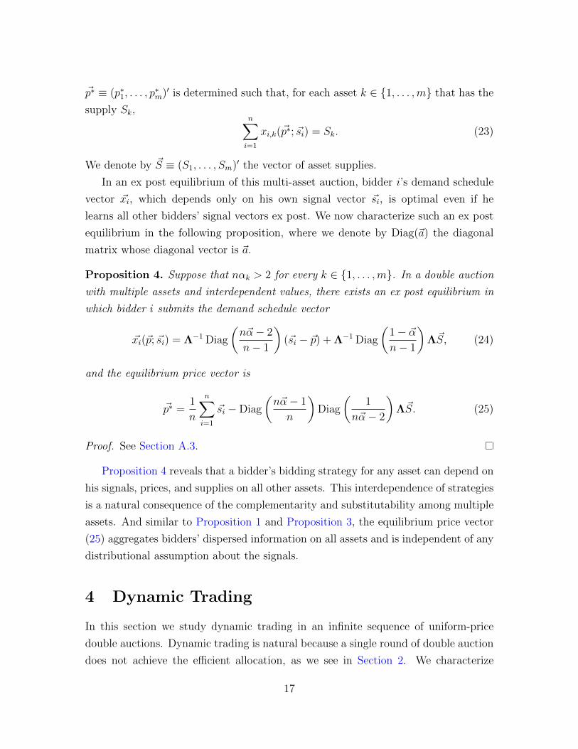
~p∗ ≡ (p∗1, . . . , p∗m)′ is determined such that, for each asset k ∈ {1, . . . ,m} that has the
supply Sk,n∑i=1
xi,k(~p∗; ~si) = Sk. (23)
We denote by ~S ≡ (S1, . . . , Sm)′ the vector of asset supplies.
In an ex post equilibrium of this multi-asset auction, bidder i’s demand schedule
vector ~xi, which depends only on his own signal vector ~si, is optimal even if he
learns all other bidders’ signal vectors ex post. We now characterize such an ex post
equilibrium in the following proposition, where we denote by Diag(~a) the diagonal
matrix whose diagonal vector is ~a.
Proposition 4. Suppose that nαk > 2 for every k ∈ {1, . . . ,m}. In a double auction
with multiple assets and interdependent values, there exists an ex post equilibrium in
which bidder i submits the demand schedule vector
~xi(~p; ~si) = Λ−1 Diag
(n~α− 2
n− 1
)(~si − ~p) + Λ−1 Diag
(1− ~αn− 1
)Λ~S, (24)
and the equilibrium price vector is
~p∗ =1
n
n∑i=1
~si −Diag
(n~α− 1
n
)Diag
(1
n~α− 2
)Λ~S. (25)
Proof. See Section A.3.
Proposition 4 reveals that a bidder’s bidding strategy for any asset can depend on
his signals, prices, and supplies on all other assets. This interdependence of strategies
is a natural consequence of the complementarity and substitutability among multiple
assets. And similar to Proposition 1 and Proposition 3, the equilibrium price vector
(25) aggregates bidders’ dispersed information on all assets and is independent of any
distributional assumption about the signals.
4 Dynamic Trading
In this section we study dynamic trading in an infinite sequence of uniform-price
double auctions. Dynamic trading is natural because a single round of double auction
does not achieve the efficient allocation, as we see in Section 2. We characterize
17

a stationary and subgame perfect ex post equilibrium, in which the allocations of
assets among the bidders converge exponentially to the efficient level as the number
of trading rounds increases.
The new element of this section is that trading occurs in repeated rounds of double
auctions at each clock time τ ∈ {0,∆, 2∆, 3∆, . . .}, where ∆ > 0 is the length of each
round of trading in clock time. The smaller is ∆, the higher is the frequency of
trading. (We later discuss the limiting behavior of the market as ∆ → 0.) Bidders
have a discounting factor of e−rτ at clock time τ , where r > 0 is the discount rate
per unit of clock time. We will refer to each trading round as a period, indexed by
t ∈ {0, 1, 2, . . .}, so the period-t auction occurs at the clock time t∆.
As in Section 2, n bidders receive private signals {si} and have interdependent
values {vi}, where vi is defined by (1). Bidders’ signals and values do not change
with time. We let zi,t be bidder i’s private inventory before the period-t auction is
held. The initial total inventory Z =∑n
i=1 zi,0 is common knowledge. For simplicity,
we assume that the external supply S is zero in each period. This implies that the
total inventory in each period t ≥ 1 is also Z.
In each period t ≥ 0, a new uniform-price double auction is held to reallocate the
asset among the bidders. In auction t, bidder i submits a demand schedule xi,t(p).
The auctioneer determines the market-clearing price p∗t by
n∑i=1
xi,t(p∗t ) = 0, (26)
and bidder i receives qi,t = xi,t(p∗t ) units of the asset at the price of p∗t . Inventories
therefore evolve according to
zi,t+1 = zi,t + qi,t. (27)
Bidder i’s utility in period t alone is
U(qi,t, p∗t ; vi, zi,t) =
(vi(zi,t + qi,t)−
1
2λ(qi,t + zi,t)
2
)∆− p∗t qi,t. (28)
Notice that in the dynamic model, we model bidder i’s value vi as a “flow utility”
per unit of clock time, so the asset’s contribution to bidder i’s utility in each period
should be weighted by the clock-time length of that period, ∆. The holding cost is
18

weighted similarly. Bidder i’s overall utility is the time-discounted sum:
Vi,t =∞∑t′=t
e−r(t′−t)∆U(qi,t′ , p
∗t′ ; vi, zi,t′). (29)
We emphasize that in period t before the new auction is held, bidder i’s infor-
mation consists of the path of his inventories {zi,t′}t′≤t and his submitted demand
schedules {xi,t′(p)}0≤t′<t, in addition to his private signal si. For notational simplic-
ity, we let bidder i’s information set at the beginning of period t be
Hi,t = {si, {zi,t′}0≤t′≤t, {xi,t′(p)}0≤t′<t} . (30)
Notice that by equations (26) and (27) a bidder can infer the previous price path
{p∗t′}t′<t from Hi,t. Bidder i’s period-t strategy, xi,t = xi,t(p;Hi,t), is measurable with
respect to Hi,t.
Definition 2. A subgame perfect ex post equilibrium consists of the strategy
profile {xj,t}1≤j≤n,t≥0 such that for every bidder i and for every path of his history
Hi,t, bidder i has no incentive to deviate from {xi,t′}t′≥t for every profile of other
bidders’ histories {Hj,t}j 6=i: for every alternative strategy {xi,t′}t′≥t,
Vi,t ({xi,t′}t′≥t, {xj,t}j 6=i,t′≥t, {Hj,t}j 6=i | Hi,t) ≥ Vi,t ({xi,t′}t′≥t, {xj,t}j 6=i,t′≥t, {Hj,t}j 6=i | Hi,t) .
As in Definition 1, the optimality condition in Definition 2 is written in terms of
the ex post utility, not the expected utility.
We now characterize a subgame perfect ex post equilibrium. This equilibrium is
stationary, that is, a bidder’s strategy only depends on his signal and current level of
inventory, but does not depend explicitly on t.
Proposition 5. Suppose that nα > 2, ∆ > 0 and r > 0. In the market with
interdependent values and dynamic trading, there exists a stationary and subgame
perfect ex post equilibrium in which bidder i submits the demand schedule
xi,t(p; si, zi,t) = a
(si −
1− e−r∆
∆p− λ(n− 1)
nα− 1zi,t +
λ(1− α)
nα− 1Z
), (31)
19
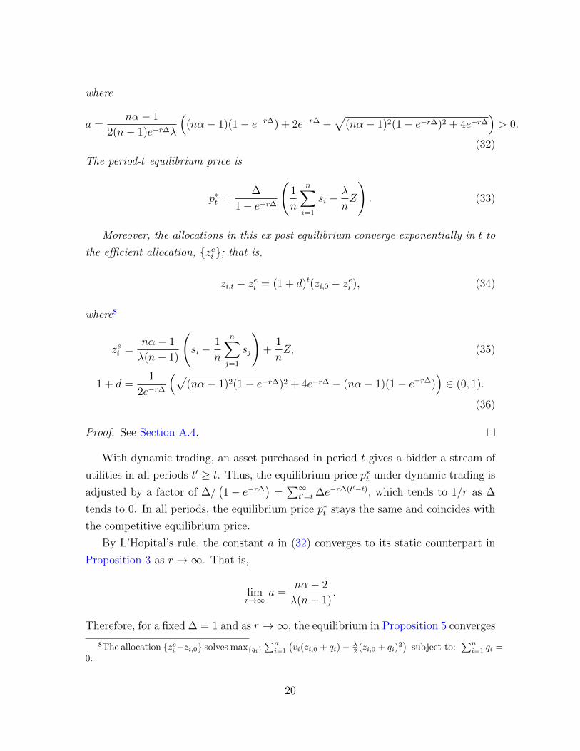
where
a =nα− 1
2(n− 1)e−r∆λ
((nα− 1)(1− e−r∆) + 2e−r∆ −
√(nα− 1)2(1− e−r∆)2 + 4e−r∆
)> 0.
(32)
The period-t equilibrium price is
p∗t =∆
1− e−r∆
(1
n
n∑i=1
si −λ
nZ
). (33)
Moreover, the allocations in this ex post equilibrium converge exponentially in t to
the efficient allocation, {zei }; that is,
zi,t − zei = (1 + d)t(zi,0 − zei ), (34)
where8
zei =nα− 1
λ(n− 1)
(si −
1
n
n∑j=1
sj
)+
1
nZ, (35)
1 + d =1
2e−r∆
(√(nα− 1)2(1− e−r∆)2 + 4e−r∆ − (nα− 1)(1− e−r∆)
)∈ (0, 1).
(36)
Proof. See Section A.4.
With dynamic trading, an asset purchased in period t gives a bidder a stream of
utilities in all periods t′ ≥ t. Thus, the equilibrium price p∗t under dynamic trading is
adjusted by a factor of ∆/(1− e−r∆
)=∑∞
t′=t ∆e−r∆(t′−t), which tends to 1/r as ∆
tends to 0. In all periods, the equilibrium price p∗t stays the same and coincides with
the competitive equilibrium price.
By L’Hopital’s rule, the constant a in (32) converges to its static counterpart in
Proposition 3 as r →∞. That is,
limr→∞
a =nα− 2
λ(n− 1).
Therefore, for a fixed ∆ = 1 and as r →∞, the equilibrium in Proposition 5 converges
8The allocation {zei−zi,0} solves max{qi}∑ni=1
(vi(zi,0 + qi)− λ
2 (zi,0 + qi)2)
subject to:∑ni=1 qi =
0.
20
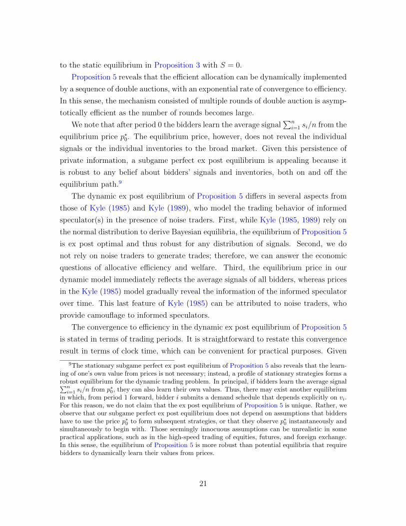
to the static equilibrium in Proposition 3 with S = 0.
Proposition 5 reveals that the efficient allocation can be dynamically implemented
by a sequence of double auctions, with an exponential rate of convergence to efficiency.
In this sense, the mechanism consisted of multiple rounds of double auction is asymp-
totically efficient as the number of rounds becomes large.
We note that after period 0 the bidders learn the average signal∑n
i=1 si/n from the
equilibrium price p∗0. The equilibrium price, however, does not reveal the individual
signals or the individual inventories to the broad market. Given this persistence of
private information, a subgame perfect ex post equilibrium is appealing because it
is robust to any belief about bidders’ signals and inventories, both on and off the
equilibrium path.9
The dynamic ex post equilibrium of Proposition 5 differs in several aspects from
those of Kyle (1985) and Kyle (1989), who model the trading behavior of informed
speculator(s) in the presence of noise traders. First, while Kyle (1985, 1989) rely on
the normal distribution to derive Bayesian equilibria, the equilibrium of Proposition 5
is ex post optimal and thus robust for any distribution of signals. Second, we do
not rely on noise traders to generate trades; therefore, we can answer the economic
questions of allocative efficiency and welfare. Third, the equilibrium price in our
dynamic model immediately reflects the average signals of all bidders, whereas prices
in the Kyle (1985) model gradually reveal the information of the informed speculator
over time. This last feature of Kyle (1985) can be attributed to noise traders, who
provide camouflage to informed speculators.
The convergence to efficiency in the dynamic ex post equilibrium of Proposition 5
is stated in terms of trading periods. It is straightforward to restate this convergence
result in terms of clock time, which can be convenient for practical purposes. Given
9The stationary subgame perfect ex post equilibrium of Proposition 5 also reveals that the learn-ing of one’s own value from prices is not necessary; instead, a profile of stationary strategies forms arobust equilibrium for the dynamic trading problem. In principal, if bidders learn the average signal∑ni=1 si/n from p∗0, they can also learn their own values. Thus, there may exist another equilibrium
in which, from period 1 forward, bidder i submits a demand schedule that depends explicitly on vi.For this reason, we do not claim that the ex post equilibrium of Proposition 5 is unique. Rather, weobserve that our subgame perfect ex post equilibrium does not depend on assumptions that biddershave to use the price p∗0 to form subsequent strategies, or that they observe p∗0 instantaneously andsimultaneously to begin with. Those seemingly innocuous assumptions can be unrealistic in somepractical applications, such as in the high-speed trading of equities, futures, and foreign exchange.In this sense, the equilibrium of Proposition 5 is more robust than potential equilibria that requirebidders to dynamically learn their values from prices.
21
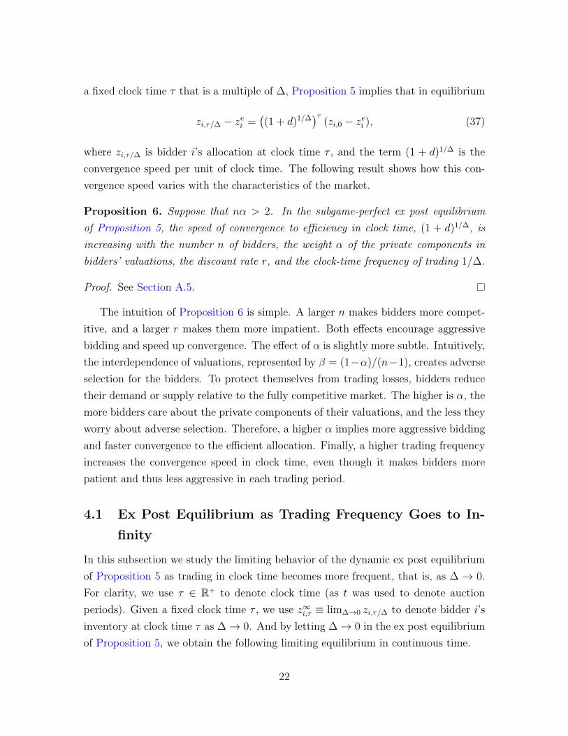
a fixed clock time τ that is a multiple of ∆, Proposition 5 implies that in equilibrium
zi,τ/∆ − zei =((1 + d)1/∆
)τ(zi,0 − zei ), (37)
where zi,τ/∆ is bidder i’s allocation at clock time τ , and the term (1 + d)1/∆ is the
convergence speed per unit of clock time. The following result shows how this con-
vergence speed varies with the characteristics of the market.
Proposition 6. Suppose that nα > 2. In the subgame-perfect ex post equilibrium
of Proposition 5, the speed of convergence to efficiency in clock time, (1 + d)1/∆, is
increasing with the number n of bidders, the weight α of the private components in
bidders’ valuations, the discount rate r, and the clock-time frequency of trading 1/∆.
Proof. See Section A.5.
The intuition of Proposition 6 is simple. A larger n makes bidders more compet-
itive, and a larger r makes them more impatient. Both effects encourage aggressive
bidding and speed up convergence. The effect of α is slightly more subtle. Intuitively,
the interdependence of valuations, represented by β = (1−α)/(n−1), creates adverse
selection for the bidders. To protect themselves from trading losses, bidders reduce
their demand or supply relative to the fully competitive market. The higher is α, the
more bidders care about the private components of their valuations, and the less they
worry about adverse selection. Therefore, a higher α implies more aggressive bidding
and faster convergence to the efficient allocation. Finally, a higher trading frequency
increases the convergence speed in clock time, even though it makes bidders more
patient and thus less aggressive in each trading period.
4.1 Ex Post Equilibrium as Trading Frequency Goes to In-
finity
In this subsection we study the limiting behavior of the dynamic ex post equilibrium
of Proposition 5 as trading in clock time becomes more frequent, that is, as ∆ → 0.
For clarity, we use τ ∈ R+ to denote clock time (as t was used to denote auction
periods). Given a fixed clock time τ , we use z∞i,τ ≡ lim∆→0 zi,τ/∆ to denote bidder i’s
inventory at clock time τ as ∆→ 0. And by letting ∆→ 0 in the ex post equilibrium
of Proposition 5, we obtain the following limiting equilibrium in continuous time.
22
Proposition 7. Suppose that nα > 2 and r > 0. As ∆ → 0, the equilibrium of
Proposition 5 converges to the following ex post equilibrium:
1. Bidder i’s equilibrium strategy is represented by a process {x∞i,τ}τ∈R+. At the
clock time τ , x∞i,τ specifies bidder i’s rate of order submission and is defined by
x∞i,τ (p; si, z∞i,τ ) = a∞
(si − rp−
λ(n− 1)
nα− 1z∞i,τ +
λ(1− α)
nα− 1Z
), (38)
where
a∞ =(nα− 1)(nα− 2)r
2λ(n− 1). (39)
Given a clock time T > 0, in equilibrium the total amount of trading by bidder
i in the clock-time interval [0, T ] is
z∞i,T − zi,0 =
∫ T
τ=0
x∞i,τ (p∗; si, z
∞i,τ )dτ. (40)
2. The equilibrium price at any clock time τ is
p∗ =1
r
(1
n
n∑i=1
si −λ
nZ
). (41)
3. Bidder i’s equilibrium allocation path {z∞i,τ}τ≥0 converges to the efficient alloca-
tion zei (given by (35)) exponentially at the rate of r(nα− 2)/2. That is, given
any clock time τ ≥ 0,
z∞i,τ − zei = e−12r(nα−2)τ (zi,0 − zei ) . (42)
Proof. See Section A.6.
One implication of Proposition 7 is that even though trading occurs continually,
in equilibrium the efficient allocation is not reached instantaneously. The delay comes
from bidders’ price impact and associated demand reduction. Although submitting
aggressive orders allows a bidder to achieve his desired allocation sooner, aggressive
bidding also moves the price against the bidder and increases his trading cost. Facing
this tradeoff, each bidders uses a finite rate of order submission in the limit. Consistent
with Proposition 6, the speed of convergence to efficiency in Proposition 7 is increasing
23
in the number of bidders n, the discount rate r, and the weight α of the private
components in bidders’ valuations.
5 Conclusion
In this paper we characterize the ex post equilibrium in a uniform-price double auction
with interdependent values. In the ex post equilibrium, a bidder’s strategy depends
only on his own private information, but he does not deviate from it even after ob-
serving the private information of other bidders. This ex post equilibrium aggregates
private information dispersed across bidders, and is robust to distributional assump-
tions and details of auction design. Under mild conditions this ex post equilibrium is
unique in the class of continuously differentiable strategy profiles. Moreover, we show
that the ex post equilibrium can be adapted to settings with private inventories and
with multiple classes of assets.
We further generalize our ex post equilibrium to a dynamic game with an infinite
sequence of double auctions. In this dynamic market, we characterize a stationary
and subgame perfect ex post equilibrium, in which the allocations of assets among
bidders converge exponentially to the efficient allocation as the number of auction
rounds increase. A key economic implication of our analysis is that a sequence of
double auctions is an asymptotically optimal mechanism that maximizes allocative
efficiency.
Appendix
A Proofs
A.1 Proof of Proposition 2
We fix an ex post equilibrium strategy (x1, . . . , xn) such that for every i, xi is con-
tinuously differentiable, ∂xi∂p
(p; si) < 0 and ∂xi∂si
(p; si) > 0. We will show that the
equilibrium demand schedule xi must be linear in si and p.
For any fixed p, we let the inverse function of xi(p; · ) be si(p; · ). That is, for any
realized allocation yi ∈ R, we have xi(p; si(p; yi)) = yi. Because xi(p; si) is strictly
24
increasing in si, si(p; yi) is strictly increasing yi. Throughout the proof, we will denote
dealer’s realized allocation by yi and his demand schedule by xi( · ; · ). With an abuse
of notation, we denote ∂xi∂p
(p; yi) ≡ ∂xi∂p
(p; si(p; yi)).
We also fix a profile of signal s = (s1, . . . , sn) ∈ (s, s)n. Let p = p∗(s) and
yi = xi(p∗(s); si). By continuity, there exists some δ > 0 such that, for any i and any
(p, yi) ∈ (p−δ, p+δ)×(yi−δ, yi+δ), there exists some s′i ∈ (s, s) such that xi(p; s′i) = yi.
In other words, every price and allocation pair in (p − δ, p + δ) × (yi − δ, yi + δ) is
“realizable” given some signal.
We will prove that there exist constants A 6= 0, B and E such that
si(p; yi) = Ayi +Bp+ E (43)
for (p, yi) ∈ (p − δ/n, p + δ/n) × (yi − δ/n, yi + δ/n), i ∈ {1, . . . , n}. Once (43) is
established, we can then rewrite
xi(p; s′i) =
s′i −Bp− EA
for p ∈ (p− δ′, p+ δ′), s′i ∈ (si− δ′, si + δ′), and i ∈ {1, . . . , n}, where δ′ > 0 is a suffi-
ciently small constant so that xi(p; s′i) ∈ (yi− δ/n, yi + δ/n) for (p, s′i) in this interval.
That is, the demand schedule xi is linear and symmetric in a neighborhood of (p, si),
for every bidder i. Once linearity and symmetry are established, the construction in
the main text preceding Proposition 1 then pins down the values of A, B and E, which
are independent of (s1, . . . , sn) and the choice of the neighborhood. Since (s1, . . . , sn)
is arbitrary, the same constants A, B, and E apply to any s = (s1, . . . , sn) ∈ (s, s)n
and p = p∗(s), which implies the uniqueness of the strategy xi(p; si).
We now proceed to prove (43). There are two cases. In Case 1, α < 1 and n ≥ 4.
In Case 2, α = 1 and n ≥ 3.
A.1.1 Case 1: α < 1 and n ≥ 4
The proof for Case 1 consists of two steps.
Step 1 of Case 1: Lemma 1 and Lemma 2 below imply equation (43).
Lemma 1. There exist functions A(p), {Bi(p)} such that
si(p; yi) = A(p)yi +Bi(p), (44)
25

holds for every p ∈ (p− δ, p+ δ) and every yi ∈ (yi − δ/n, yi + δ/n), 1 ≤ i ≤ n.
Proof. This lemma is proved in Step 2 of Case 1. For this lemma we need the condition
that n ≥ 4; in the rest of the proof n ≥ 3 suffices.
Lemma 2. Suppose that l ≥ 2 and that
l∑i=1
fi(p; yi) = fl+1
(p,
l∑i=1
yi
), (45)
for every p ∈ P and (y1, . . . , yl) ∈∏l
i=1 Yi, where Yi is an open subset of R, fi is
differentiable and P is an arbitrary set. Then there exists function C(p) and {Di(p)}such that
fi(p; yi) = C(p)yi +Di(p)
holds for every i ∈ {1, . . . , l}, p ∈ P and yi ∈ Yi.
Proof. We differentiate (45) with respect to yi and to yj, where i, j ∈ {1, 2, . . . , l},and obtain
∂fi∂yi
(p; yi) =∂fl+1
∂yi
(p;
l∑j=1
yj
)=∂fj∂yj
(p; yj)
for any yi ∈ Yi and yj ∈ Yj. Because (y1, . . . , yl) are arbitrary, the partial derivatives
above cannot depend on any particular yi. Thus, there exists some function C(p)
such that ∂fi∂yi
(p; yi) = C(p) for all yi. Lemma 2 then follows.
In Step 1 of the proof of Case 1 of Proposition 2, we show that Lemma 1 and
Lemma 2 imply equation (43). Let us first rewrite bidder i’s ex post first-order
condition as:
− yi +
(αsi(p; yi) + β
∑j 6=i
sj(p; yj)− p− λyi
)(−∑j 6=i
∂xj∂p
(p; yj)
)= 0, (46)
where yn = S −∑n−1
j=1 yj, p ∈ (p− δ, p+ δ) and yj ∈ (yj − δ/n, yj + δ/n). 10
Our strategy is to repeatedly apply Lemma 1 and Lemma 2 to (46) in order to
arrive at (43).
10We restrict yj to (yj − δ/n, yj + δ/n) so that yn = S −∑n−1j=1 yj ∈ (yn − δ, yn + δ), and as a
result s(p; yn) and ∂xn
∂yn(p; yn) are well-defined.
26
First, we plug the functional form of Lemma 1 into (46). Without loss of generality,
we let i = n and rewrite (46) as
n−1∑j=1
∂xj∂p
(p; yj)︸ ︷︷ ︸left-hand side of (45)
= − yn
α(A(p)yn +Bn(p)) + β∑n−1
j=1 (A(p)yj +Bj(p))− p− λyn︸ ︷︷ ︸right-hand side of (45)
.
Applying Lemma 2 to the above equation, we see that there exist functions C(p) and
{Dj(p)} such that∂xj∂p
(p; yj) = C(p)yj +Dj(p), (47)
for j ∈ {1, . . . , n − 1}. Note that we have used the condition n ≥ 3 when applying
Lemma 1.
By the same argument, we apply Lemma 2 to (46) for i = 1, and conclude that
(47) holds for j = n as well.
Using (44) and (47), we rewrite bidder i’s ex post first-order condition as:((α− β)si(p; yi) + β
(A(p)S +
n∑j=1
Bj(p)
)− p− λyi
)(−C(p)(S − yi)−
∑j 6=i
Dj(p)
)−yi = 0.
(48)
Solving for si(p; yi) in terms of p and yi from equation (48), we see that for the so-
lution to be consistent with (44), we must have C(p) = 0. Otherwise, i.e. if C(p) 6= 0,
then (48) implies that si(p; yi) contains the term yi/(−C(p)(S − yi)−
∑j 6=iDj(p)
),
contradicting the linear form of Lemma 1.
Inverting (44), we see that xi(p; si) = (si−Bi(p))/A(p). Therefore, for ∂xi∂p
(p; si) to
be independent of si (i.e., C(p) = 0), A(p) must be a constant function, i.e. A(p) = A
for some constant A ∈ R. This implies that
Di(p) = −B′i(p)
A, (49)
by the definition of Di(p) in (47).
Given C(p) = 0 and A(p) = A, (48) can be rewritten as
(α− β)si(p; yi) + β
(AS +
n∑j=1
Bj(p)
)− p− λyi −
yi−∑
j 6=iDj(p)= 0. (50)
27

For (50) to be consistent with si(p; yi) = Ayi +Bi(p), we must have that Dj(p) = Dj
for some constants Dj, j ∈ {1, . . . , n}, and that
1∑j 6=iDj
=1∑
j 6=i′ Dj
, for all i 6= i′,
which implies that for all i, Di ≡ D for some constant D.
By (49), this means that Bi(p) = Bp+Ei where B = −DA. Finally, (50) implies
that Ei = Ej = E for some constant E as well.
Hence, we have shown that Lemma 1 implies (43). This completes Step 1 of the
proof of Case 1 of Proposition 2. In Step 2 below, we prove Lemma 1.
Step 2 of Case 1: Proof of Lemma 1.
Bidder n’s ex post first order condition can be written as:
n−1∑j=1
∂xj∂p
(p; yj) = − yn
αsn(p; yn) + β∑n−1
j=1 sj(p; yj)− p− λyn, (51)
where yn = S −∑n−1
j=1 yj. Differentiate (51) with respect to yi gives:
∂
∂yi
(∂xi∂p
(p; yi)
)=
Γ(y1, . . . , yn−1) + yn
(−α ∂sn
∂yn(p; yn) + β ∂s1
∂y1(p; y1) + λ
)Γ(y1, . . . , yn−1)2
, (52)
where
Γ(y1, . . . , yn−1) = αsn(p; yn) + βn−1∑j=1
sj(p; yj)− p− λyn. (53)
Solving for Γ(y1, . . . , yn−1) in (52), we get
Γ(y1, . . . , yn−1) = ρi
(yi,
n−1∑j=1
yj
)(54)
for some function ρi, i ∈ {1, 2, . . . , n− 1}.We let ρi,1 be the partial derivative of ρi with respect to its first argument, and
let ρi,2 be the partial derivative of ρi with respect to its second argument. For each
pair of distinct i, k ∈ {1, . . . , n− 1}, differentiating (54) with respect to yi and yk, we
28
have
dΓ(y1, . . . , yn−1)
dyi= ρi,1 + ρi,2 = ρk,2,
dΓ(y1, . . . , yn−1)
dyk= ρk,1 + ρk,2 = ρi,2,
which imply that for all i 6= k ∈ {1, . . . , n− 1},
ρi,1 + ρk,1 = 0. (55)
Clearly, (55) together with n ≥ 4 imply that ρi,1 = −ρi,1, i.e., ρi,1 = 0 for all
i ∈ {1, . . . , n− 1}. That is, each ρi is only a function of its second argument:
ρi
(yi,
n−1∑j=1
yj
)= ρi
(n−1∑j=1
yj
). (56)
Then, using (53), (54) and (56) for i = 1, we have
βn−1∑j=1
sj(p; yj) = ρ1
(n−1∑j=1
yj
)+ p+ λyn − αsn(p; yn). (57)
Applying Lemma 2 to (57) (recall that yn = S −∑n−1
j=1 yj), we conclude that, for all
j ∈ {1, . . . , n− 1},sj(p; yj) = A(p)yj +Bj(p). (58)
Finally, we repeat this argument to bidder 1’s ex post first-order condition and con-
clude that (58) holds for j = n as well. This concludes the proof of Lemma 1.
A.1.2 Case 2: α = 1 and n ≥ 3
We now prove Case 2 of Proposition 2. Bidder n’s ex post first order condition in
this case is:n−1∑j=1
∂xj∂p
(p; yj) =−yn
sn(p∗; yn)− p− λyn, (59)
for every p ∈ (p− δ, p+ δ) and (y1, . . . , yn−1) ∈∏n−1
j=1 (yj − δ/n, yj + δ/n), and where
yn = S −∑n−1
j=1 yj.
29
Applying Lemma 2 to (59) gives:
∂xj∂p
(p; yj) = C(p)yj +Dj(p), (60)
for j ∈ {1, . . . , n − 1}. Applying Lemma 2 to the ex post first-order condition of
bidder 1 shows that (60) holds for j = n as well.
Substituting (60) back into the first-order condition (59), we obtain:
(si(p; yi)− p− λyi)
(−C(p)(S − yi)−
∑j 6=i
Dj(p)
)− yi = 0,
which can be rewritten as:
∂xi∂p
(p; yi) = C(p)yi +Di(p) =yi
si(p; yi)− p− λyi+ C(p)S +
n∑j=1
Dj(p). (61)
We claim that C(p) = 0. Suppose for contradiction that C(p) 6= 0. Then matching
the coefficient of yi in (61), we must have si(p; yi) = λyi + Bi(p) for some function
Bi(p). But this implies that ∂xi∂p
(p; yi) = −B′i(p)/λ, which is independent of yi. This
implies C(p) = 0, a contradiction. Thus, C(p) = 0.
Then, (61) implies that si(p; yi)− p = Ai(p)yi for some function Ai(p). And since∂xi∂p
(p; yi) is independent of yi, Ai(p) must be a constant function, i.e., si(p; yi)− p =
Aiyi for some Ai ∈ R. Substitute this back to (61) gives:
∂xi∂p
(p; yi) = − 1
Ai=
1
Ai − λ−
n∑j=1
1
Aj,
which implies1
Ai − λ− 1
Aj − λ=
1
Aj− 1
Ai, for all i 6= j,
which is only possible if Ai = Aj ≡ A ∈ R for all i 6= j. Thus, si(p; yi) − p = Ayi,
which concludes the proof of this case.
A.2 Proof of Proposition 3
We first verify the ex post equilibrium of Proposition 3. Then, we prove uniqueness.
30

With inventory and given other bidders’ demand schedules, bidder i’s utility is
Πi(p) =
(S −
∑j 6=i
xj(p; sj, zj)
)(αsi + β
∑j 6=i
sj − p
)− 1
2λ
(zi + S −
∑j 6=i
xj(p; sj, zj)
)2
.
Taking the first-order condition of Πi(p), we obtain
0 = Π′i(p∗) = −xi(p∗; si, zi) +
(−∑j 6=i
∂xj∂p
(p∗; sj, zj)
)[αsi + β
∑j 6=i
sj − p∗ − λ (zi + xi(p∗; si, zi))
].
(62)
As before, we conjecture a linear demand schedule
xj(p; sj, zj) = asj − bp+ cS + dzj + eZ,
and write
∑j 6=i
sj =1
a
[∑j 6=i
xj(p∗; sj, zj) + (n− 1)bp∗ − (n− 1)cS − d
∑j 6=i
zj − (n− 1)eZ
]
=1
a[S − xi(p∗; si, zi) + (n− 1)bp∗ − (n− 1)cS − d(Z − zi)− (n− 1)eZ] .
Substituting the above expression into (62) and rearranging, we have
xi(p∗; si, zi) = [1 + λ(n− 1)b+ β(n− 1)b/a]−1 · (n− 1)b
· {αsi − [1− β(n− 1)b/a] p∗ + S [1− (n− 1)c] β/a
+ (βd/a− λ)zi − Z[d+ (n− 1)e]β/a}
≡ asi − bp∗ + cS + dzi + eZ.
Matching the coefficients and using the normalization that α+ (n−1)β = 1, we solve
a = b =1
λ· nα− 2
n− 1, c =
1− αn− 1
, d = −nα− 2
nα− 1, e =
1− αn− 1
· nα− 2
nα− 1.
We now turn to uniqueness. For a fixed ex post equilibrium (x1, . . . , xn) and a
31

profile of inventories z = (z1, . . . , zn), the ex post first-order condition for bidder i is:
−xi(p∗; si, zi)+
(αsi + β
∑j 6=i
sj − p∗ − λ(zi + xi(p∗; si, zi))
)(−∑j 6=i
∂xj∂p
(p∗; sj, zj)
)= 0.
Under the same conditions stated in Proposition 2, we apply the reasoning in the proof
of Proposition 2 to the fixed profile z and conclude that in any ex post equilibrium,
xi(p∗; si, zi) = a(z)si − b(z)p∗ + d(z)zi + C(z),
for some functions a(z), b(z), d(z), and C(z). The calculations above show that these
functions are independent of z and thus are constants. The uniqueness of the ex post
equilibrium follows.
A.3 Proof of Proposition 4
Suppose that other bidders j 6= i use the strategy {~xj( · ; ~sj)}j 6=i. For fixed signals
(~s1, . . . , ~sn), bidder i’s utility at the price vector ~p is
Πi(~p) =
(Diag(~α)~si + Diag(~β)
∑j 6=i
~sj − ~p
)′(~S −
∑j 6=i
~xj(~p; ~sj)
)
− 1
2
(~S −
∑j 6=i
~xj(~p; ~sj)
)′Λ
(~S −
∑j 6=i
~xj(~p; ~sj)
).
Bidder i’s ex-post first-order condition is that the gradient of Πi vanishes at the
market-clearing prices ~p∗, i.e.,
dΠi(~p∗)
d~p= −~xi(~p∗; ~si) +
(−∑j 6=i
∂ ~xj(~p∗; ~sj)
∂~p
)′(Diag(~α)~si + Diag(~β)
∑j 6=i
~sj − ~p∗ −Λ~xi(~p∗; ~si)
)= 0,
(63)
where∂ ~xj( ~p∗;~sj)
∂~pis an m-by-m matrix of partial derivatives.
We conjecture that bidders use linear symmetric demand schedules of the form:
~xi(~p; ~si) = B(~si − ~p) + C~S,
32
where B and C are m-by-m matrices. Furthermore, we assume that B is symmetric
and invertible.
These demand schedules yield the market-clearing price vector of
~p∗ =1
n
n∑i=1
~si + B−1
(C− 1
nI
)~S.
where I is the identity matrix. Substituting the expressions of ~xj and ~p∗ into (63)
and rearranging, we have:
(I + (n− 1)BΛ) (B(~si−~p∗)+C~S) = (n−1)B
(Diag(~α− ~β)(~si − ~p∗)−Diag(n~β)B−1
(C− 1
nI
)~S
).
Matching coefficients with our conjecture, we obtain:
B = Λ−1 Diag
(n~α− 2
n− 1
),
C = Λ−1 Diag
(1− ~αn− 1
)Λ.
A.4 Proof of Proposition 5
In this proof, we first construct the stationary and subgame perfect ex post equilib-
rium of Proposition 5, and then show that the allocation path in this equilibrium
converges to the efficient allocation as the trading round t→∞.
We conjecture that bidders use the stationary and symmetric strategy:
xi,t(p; si, zi,t) = asi − bp+ dzi,t + fZ. (64)
We let p∗ be the market-clearing price in every period as determined by the con-
jectured strategy (64):
an∑j=1
sj − bnp∗ + (d+ nf)Z = 0. (65)
For the simplicity of notation we write xi,t(p∗; si, zi,t) as xi,t.
We want to construct the strategy in (64) so that for any fixed profiles (s1, . . . , sn)
and (z1,t, . . . , zn,t), every bidder i does not have an incentive to deviate from this
33

strategy in period t if he anticipates that (i) others are using this strategy from
period t on, and (ii) he himself will return to this strategy from period t + 1 and
onwards. Then, by the single-deviation principle, this symmetric strategy profile is a
subgame perfect ex post equilibrium.
Bidder i’s ex post first-order condition (with respect to p∗t ) in period t is:(−∑j 6=i
∂xj,t∂p
(p∗t ; sj, zj,t)
)·
[∆
(vi − λ(xi,t + zi,t) +
∞∑k=1
e−rk∆∂(zi,t+k + xi,t+k)
∂xi,t(vi − λ(zi,t+k + xi,t+k))
)
− p∗t −∞∑k=1
e−rk∆∂xi,t+k∂xi,t
p∗t+k
]− xi,t −
∞∑k=1
e−rk∆ xi,t+k∂p∗t+k∂p∗t
= 0.
(66)
If bidders follow the conjectured strategy in (64) from period t + 1 and onwards,
then we have the following evolution of inventories and prices, for k ≥ 1:
zi,t+k + xi,t+k = (asi − bp∗ + fZ)(1 + (1 + d) + · · ·+ (1 + d)k−1
)+ (1 + d)k(xi,t + zi,t)
= (asi − bp∗ + fZ)
(1
−d− (1 + d)k
−d
)+ (1 + d)k(xi,t + zi,t), (67)
p∗t+k = p∗,
where p∗ is defined in (65). This implies that
∂(zi,t+k + xi,t+k)
∂xi,t= (1 + d)k, (68)
∂xi,t+k∂xi,t
= (1 + d)k−1d, (69)
∂p∗t+k∂p∗t
=∂p∗t+k∂xi,t
= 0. (70)
Given the conjectured strategy in (64) and the derivatives in (68), (69) and (70),
34
the ex post first order condition in (66) becomes:
(n− 1)b
[∆
(vi − λ(xi,t + zi,t) +
∞∑k=1
e−rk∆(1 + d)k(vi − λ(zi,t+k + xi,t+k))
)
− p∗ −∞∑k=1
e−rk∆(1 + d)k−1d p∗
]− xi,t = 0. (71)
Averaging Equation (71) across all bidders and using the fact that∑n
i=1 xi,t+k = 0
and∑n
i=1 zi,t+k = Z, we get:
p∗ =∆
1− e−r∆
(s− λ
nZ
), (72)
where
s ≡ 1
n
n∑i=1
si.
Therefore, in (64) we must have
b =1− e−r∆
∆a, (73)
aλ
n+d
n+ f = 0.
Substituting (67), (72) and (73) into the first-order condition (71) gives:
(n− 1)(1− e−r∆)a
[1
1− e−r∆(1 + d)
(vi − s+
λ
nZ
)(74)
−∞∑k=1
λe−rk∆(1 + d)k(
1
−d− (1 + d)k
−d
)(a(si − s)−
d
nZ
)
− λ
1− e−r∆(1 + d)2(xi,t + zi,t)
]− xi,t = 0.
35
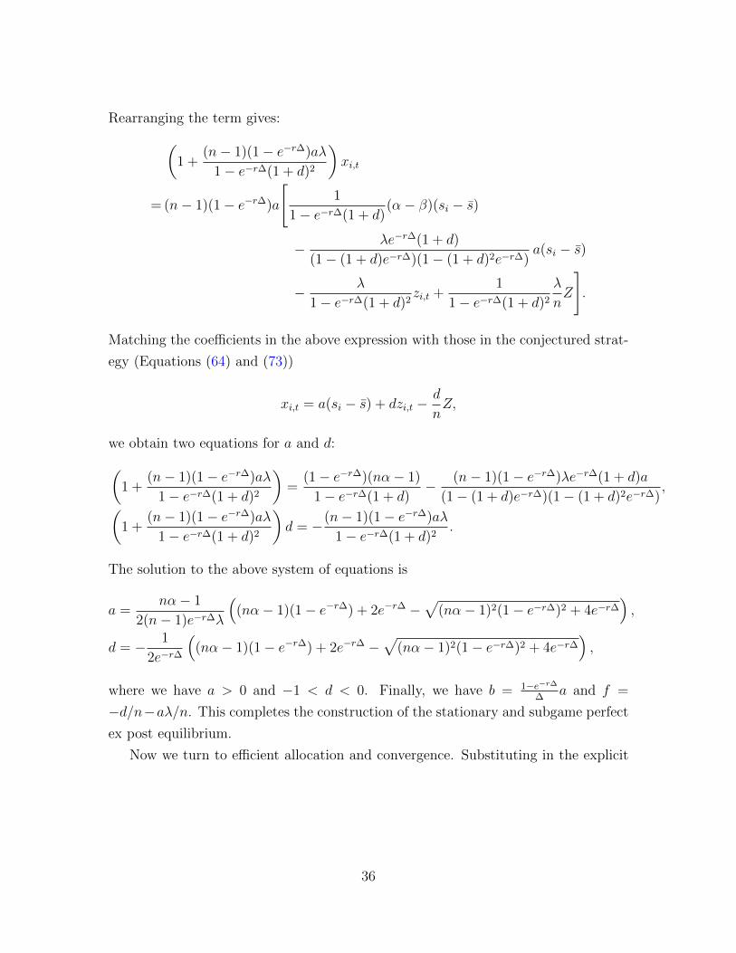
Rearranging the term gives:(1 +
(n− 1)(1− e−r∆)aλ
1− e−r∆(1 + d)2
)xi,t
= (n− 1)(1− e−r∆)a
[1
1− e−r∆(1 + d)(α− β)(si − s)
− λe−r∆(1 + d)
(1− (1 + d)e−r∆)(1− (1 + d)2e−r∆)a(si − s)
− λ
1− e−r∆(1 + d)2zi,t +
1
1− e−r∆(1 + d)2
λ
nZ
].
Matching the coefficients in the above expression with those in the conjectured strat-
egy (Equations (64) and (73))
xi,t = a(si − s) + dzi,t −d
nZ,
we obtain two equations for a and d:(1 +
(n− 1)(1− e−r∆)aλ
1− e−r∆(1 + d)2
)=
(1− e−r∆)(nα− 1)
1− e−r∆(1 + d)− (n− 1)(1− e−r∆)λe−r∆(1 + d)a
(1− (1 + d)e−r∆)(1− (1 + d)2e−r∆),(
1 +(n− 1)(1− e−r∆)aλ
1− e−r∆(1 + d)2
)d = −(n− 1)(1− e−r∆)aλ
1− e−r∆(1 + d)2.
The solution to the above system of equations is
a =nα− 1
2(n− 1)e−r∆λ
((nα− 1)(1− e−r∆) + 2e−r∆ −
√(nα− 1)2(1− e−r∆)2 + 4e−r∆
),
d = − 1
2e−r∆
((nα− 1)(1− e−r∆) + 2e−r∆ −
√(nα− 1)2(1− e−r∆)2 + 4e−r∆
),
where we have a > 0 and −1 < d < 0. Finally, we have b = 1−e−r∆
∆a and f =
−d/n−aλ/n. This completes the construction of the stationary and subgame perfect
ex post equilibrium.
Now we turn to efficient allocation and convergence. Substituting in the explicit
36

expressions for a, b, d, and f , (67) becomes:
zi,t+k+1 =
(a(si − s)−
d
nZ
)(1
−d− (1 + d)k
−d
)+ (1 + d)kzi,t+1
= zei (1− (1 + d)k) + (1 + d)kzi,t+1,
which can be rewritten as
zi,t+k+1 − zei = (1 + d)k(zi,t+1 − zei ),
where
zei =nα− 1
λ(n− 1)(si − s) +
Z
n.
To see that {zei } is the efficient allocation in the dynamic setting, note that by
Jensen’s inequality we have:
(1−e−r∆)∞∑t=0
e−rt∆(
(zi,t + qi,t)vi −λ
2(zi,t + qi,t)
2
)≤ (zi,0+q′i)vi−
λ
2(zi,0+q′i)
2, (75)
where
q′i = (1− e−r∆)∞∑t=0
e−rt∆(zi,t + qi,t)− zi,0.
It is easy to verify that
qei ≡ zei − zi,0, i ∈ {1, . . . , n}
solves:
max{qi}
n∑i=1
(vi(zi,0 + qi)−
λ
2(zi,0 + qi)
2
)subject to:
n∑i=1
qi = 0.
Therefore, by (75), qi,0 = qei and qi,t = 0, t ≥ 1 and i ∈ {1, . . . , n} solve:
max{qi,t}
n∑i=1
∞∑t=0
e−rt∆(vi(zi,t + qi,t)−
λ
2(zi,t + qi,t)
2
)∆
subject to:n∑j=1
qj,t = 0, zi,t+1 = zi,t + qi,t, for every i ∈ {1, . . . , n} and t ≥ 0.
That is, {zei } is the efficient allocation.
37
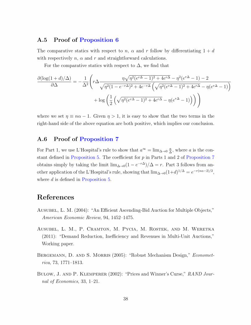
A.5 Proof of Proposition 6
The comparative statics with respect to n, α and r follow by differentiating 1 + d
with respectively n, α and r and straightforward calculations.
For the comparative statics with respect to ∆, we find that
∂(log(1 + d)/∆)
∂∆= − 1
∆2
(r∆
η√η2(er∆ − 1)2 + 4er∆ − η2(er∆ − 1)− 2√
η2(1− e−r∆)2 + 4e−r∆(√
η2(er∆ − 1)2 + 4er∆ − η(er∆ − 1))
+ log
(1
2
(√η2(er∆ − 1)2 + 4er∆ − η(er∆ − 1)
)))
where we set η ≡ nα − 1. Given η > 1, it is easy to show that the two terms in the
right-hand side of the above equation are both positive, which implies our conclusion.
A.6 Proof of Proposition 7
For Part 1, we use L’Hospital’s rule to show that a∞ = lim∆→0a∆
, where a is the con-
stant defined in Proposition 5. The coefficient for p in Parts 1 and 2 of Proposition 7
obtains simply by taking the limit lim∆→0(1− e−r∆)/∆ = r. Part 3 follows from an-
other application of the L’Hospital’s rule, showing that lim∆→0(1+d)1/∆ = e−r(nα−2)/2,
where d is defined in Proposition 5.
References
Ausubel, L. M. (2004): “An Efficient Ascending-Bid Auction for Multiple Objects,”
American Economic Review, 94, 1452–1475.
Ausubel, L. M., P. Cramton, M. Pycia, M. Rostek, and M. Weretka
(2011): “Demand Reduction, Inefficiency and Revenues in Multi-Unit Auctions,”
Working paper.
Bergemann, D. and S. Morris (2005): “Robust Mechanism Design,” Economet-
rica, 73, 1771–1813.
Bulow, J. and P. Klemperer (2002): “Prices and Winner’s Curse,” RAND Jour-
nal of Economics, 33, 1–21.
38

Cremer, J. and R. P. McLean (1985): “Optimal Selling Strategies under Un-
certainty for a Discriminating Monopolist when Demands are Interdependent,”
Econometrica, 53, 345–361.
Cripps, M. W. and J. M. Swinkels (2006): “Efficiency of Large Double Auc-
tions,” Econometrica, 74, 47–92.
Dasgupta, P. and E. Maskin (2000): “Efficient Auctions,” Quarterly Journal of
Economics, 115, 341–388.
Du, S. and H. Zhu (2012): “Are CDS Auctions Biased?” Working paper.
Fudenberg, D. and Y. Yamamoto (2011): “Learning from Private Information
in Noisy Repeated Games,” Journal of Economic Theory, 146, 1733–1769.
Grossman, S. (1976): “On the Efficiency of Competitive Stock Markets Where
Trades Have Diverse Information,” Journal of Finance, 31, 573–585.
——— (1981): “An Introduction to the Theory of Rational Expectations Under
Asymmetric Info,” Review of Economic Studies, 48, 541–559.
Holmstrom, B. and R. B. Myerson (1983): “Efficient and Durable Decision
Rules with Incomplete Information,” Econometrica, 51, 1799–1819.
Horner, J. and S. Lovo (2009): “Belief-Free Equilibria in Games with Incomplete
Information,” Econometrica, 77, 453–487.
Jehiel, P., M. Meyer-Ter-Vehn, B. Moldovanu, and W. R. Zame (2006):
“The Limits of Ex Post Implementation,” Econometrica, 74, 585–610.
Kazumori, E. (2012): “Information Aggregation in Large Double Auctions with
Interdependent Values,” Working paper.
Klemperer, P. D. and M. A. Meyer (1989): “Supply Function Equilibria in
Oligopoly under Uncertainty,” Econometrica, 57, 1243–1277.
Kremer, I. (2002): “Information Aggregation in Common Value Auctions,” Econo-
metrica, 70, 1675–1682.
Kyle, A. S. (1985): “Continuous Auctions and Insider Trading,” Econometrica, 53,
1315–1335.
39

——— (1989): “Informed Speculation with Imperfect Competition,” Review of Eco-
nomic Studies, 56, 317–355.
Milgrom, P. (1981): “Rational Expectations, Information Acquisition, and Com-
petitive Bidding,” Econometrica, 49, 921–943.
Milgrom, P. R. (1979): “A Convergence Theorem for Competitive Bidding with
Differential Information,” Econometrica, 47, 679–688.
Perry, M. and P. J. Reny (2002): “An Efficient Auction,” Econometrica, 70,
1199–1212.
——— (2005): “An Efficient Multi-Unit Ascending Auction,” Review of Economic
Studies, 72, 567–592.
Reny, P. J. and M. Perry (2006): “Toward a Strategic Foundation for Rational
Expectations Equilibrium,” Econometrica, 74, 1231–1269.
Rochet, J.-C. and J.-L. Vila (1994): “Insider Trading without Normality,” Re-
view of Economic Studies, 61, 131–152.
Rostek, M. and M. Weretka (2011): “Dynamic Thin Markets,” Working paper.
——— (2012): “Price Inference in Small Markets,” Econometrica, 80, 687–711.
Rustichini, A., M. Satterthwaite, and S. R. Williams (1994): “Convergence
to Efficiency in a Simple Market with Incomplete Information,” Econometrica, 62,
1041–1063.
Vives, X. (2011): “Strategic Supply Function Competition with Private Informa-
tion,” Econometrica, 79, 1919–1966.
Wilson, R. (1977): “A Bidding Model of Perfect Competition,” Review of Economic
Studies, 44, 511–518.
——— (1979): “Auctions of Shares,” Quarterly Journal of Economics, 93, 675–689.
——— (1987): “Game-Theoretic Analyses of Trading Processes,” in Advances in
Economic Theory: Fifth World Congress, ed. by T. Bewley, Cambridge University
Press, 33–70.
40