exact local whittle estimation of fractional …korora.econ.yale.edu/phillips/pubs/art/p1156.pdf ·...

EXACT LOCAL WHITTLE ESTIMATION OF FRACTIONAL INTEGRATION

BY

KATSUMI SHIMOTSU AND PETER C. B. PHILLIPS

COWLES FOUNDATION PAPER NO. 1156

COWLES FOUNDATION FOR RESEARCH IN ECONOMICS YALE UNIVERSITY

Box 208281 New Haven, Connecticut 06520-8281

2006

http://cowles.econ.yale.edu/

The Annals of Statistics2005, Vol. 33, No. 4, 1890–1933DOI 10.1214/009053605000000309© Institute of Mathematical Statistics, 2005

EXACT LOCAL WHITTLE ESTIMATION OFFRACTIONAL INTEGRATION

BY KATSUMI SHIMOTSU1 AND PETER C. B. PHILLIPS2

Queen’s University and Yale University,University of Auckland and University of York

An exact form of the local Whittle likelihood is studied with theintent of developing a general-purpose estimation procedure for the memoryparameter (d) that does not rely on tapering or differencing prefilters. Theresulting exact local Whittle estimator is shown to be consistent and to havethe same N(0, 1

4 ) limit distribution for all values of d if the optimizationcovers an interval of width less than 9

2 and the initial value of the process isknown.

1. Introduction. Semiparametric estimation of the memory parameter (d) infractionally integrated (I (d)) time series is appealing in empirical work because ofthe general treatment of the short-memory component that it affords. Two commonstatistical procedures in this class are log-periodogram (LP) regression [1, 10]and local Whittle (LW) estimation [5, 11]. LW estimation is known to be moreefficient than LP regression in the stationary (|d| < 1

2) case, although numericaloptimization methods are needed in the calculation. Outside the stationary region,it is known that the asymptotic theory for the LW estimator is discontinuous atd = 3

4 and again at d = 1, is awkward to use because of nonnormal limit theoryand, worst of all, the estimator is inconsistent when d > 1 [8]. Thus, the LWestimator is not a good general-purpose estimator when the value of d may take onvalues in the nonstationary zone beyond 3

4 . Similar comments apply in the case ofLP estimation [4].

To extend the range of application of these semiparametric methods, datadifferencing and data tapering have been suggested [3, 15]. These methodshave the advantage that they are easy to implement and they make use ofexisting algorithms once the data filtering has been carried out. Differencing hasthe disadvantage that prior information is needed on the appropriate order ofdifferencing. Tapering has the disadvantage that the filter distorts the trajectory ofthe data and inflates the asymptotic variance. As a consequence, there is presently

Received March 2002; revised July 2004.1Supported by ESRC Grant R000223629.2Supported by NSF Grant SES-00-92509.AMS 2000 subject classification. 62M10.Key words and phrases. Discrete Fourier transform, fractional integration, long memory, nonsta-

tionarity, semiparametric estimation, Whittle likelihood.

1890

EXACT LOCAL WHITTLE ESTIMATION 1891

no general-purpose efficient estimation procedure when the value of d may takeon values in the nonstationary zone beyond 3

4 .The present paper studies an exact form of the local Whittle estimator which

does not rely on differencing or tapering and which seems to offer a good general-purpose estimation procedure for the memory parameter that applies throughoutthe stationary and nonstationary regions of d . The estimator, which we call theexact LW estimator, is shown to be consistent and to have N(0, 1

4) limit distributionwhen the optimization covers an interval of width less than 9

2 . The exact LWestimator therefore has the same limit theory as the LW estimator has for stationaryvalues of d . The approach seems to offer a useful alternative for applied researcherswho are looking for a general-purpose estimator and want to allow for a substantialrange of stationary and nonstationary possibilities for d . The method has thefurther advantage that it provides a basis for constructing asymptotic confidenceintervals for d that are valid irrespective of the true value of the memory parameter.

The exact LW estimator given here assumes the initial value of the data tobe known. This restriction can be removed by estimating it along with d , asshown by Shimotsu [14]. Also, computation of the estimator involves a numericaloptimization that is more demanding than conventional LW estimation. Ourexperience from simulations indicates that the computation time required is aboutten times that of the LW estimator and is well within the capabilities of a smallnotebook computer.

2. Exact local Whittle estimation. We consider the fractional process Xt

generated by the model

(1 − L)d0Xt = utI {t ≥ 1}, t = 0,±1, . . . ,(1)

where I {·} is the indicator function and ut is stationary with zero mean and spectraldensity fu(λ) ∼ G0 as λ → 0. Expanding the binomial in (1) gives the form

t∑k=0

(−d0)k

k! Xt−k = utI {t ≥ 1},(2)

where

(d0)k = �(d0 + k)

�(d0)= (d0)(d0 + 1) · · · (d0 + k − 1)

is Pochhammer’s symbol for the forward factorial function and �(·) is the gammafunction. When d0 is a positive integer, the series in (2) terminates, giving the usualformulae for the model (1) in terms of differences and higher-order differencesof Xt. An alternative form for Xt is obtained by inversion of (1), giving a validrepresentation for all values of d0,

Xt = (1 − L)−d0utI {t ≥ 1} =t−1∑k=0

(d0)k

k! ut−k.(3)

1892 K. SHIMOTSU AND P. C. B. PHILLIPS

Define the discrete Fourier transform (d.f.t.) and the periodogram of a time seriesat evaluated at frequency λ as

wa(λ) = (2πn)−1/2n∑

t=1

ateitλ,

Ia(λ) = |wa(λ)|2.

2.1. Exact local Whittle likelihood and estimator. We start with the likelihoodfunction of the stationary innovation ut . The (negative) Whittle likelihood of ut

based on frequencies up to λm and up to scale multiplication is

m∑j=1

logfu(λj ) +m∑

j=1

Iu(λj )

fu(λj ), λj = 2πj

n,(4)

where m is some integer less than n. We want to transform the likelihoodfunction (4) to be data dependent.

If |d0| < 12 , it is known that Iu(λj ) can be approximated by λ

2d0j Ix(λj )

[10, 12]. Therefore, if one views Iu(λj ) as the j th observation of ut in the

frequency domain, replacing Iu(λj ) in (4) with λ2d0j Ix(λj ) and adding the Jacobian∑m

j=1 logλ−2dj to (4) makes it data dependent. Indeed, the resulting objective

function coincides with that of the LW estimator.However, when d0 takes a larger value, in particular when |d0| > 1, λ

2d0j Ix(λj )

no longer provides a good approximation of Iu(λj ). In this paper, we proposeto use a “corrected” d.f.t. of Xt that can approximate Iu(λj ) and validlytransform (4) in such cases. Lemma 5.1 in Section 5 provides the necessaryalgebraic relationship for these quantities for any value of d0, namely,

Iu(λj ) = I�d0x(λj ) = |Dn(eiλj ;d0)|2|vx(λj ;d0)|2,

(5)vx(λj ;d) = wx(λj ) − Dn(e

iλj ;d)−1(2πn)−1/2Xλj n(d),

where

Dn(eiλ;d) =

n∑k=0

(−d)k

k! eikλ

and

Xλn(d) =n−1∑p=0

dλpe−ipλXn−p with dλp =n∑

k=p+1

(−d)k

k! eikλ.

The function vx(λj ;d0) in (5) adds a correction term that involves Xλj n(d0)

to the d.f.t. wx(λj ), which ensures that the relationship (5) holds exactly forall d0. Accordingly, we may interpret vx(λj ;d0) as a well-suited proxy for the


j th frequency domain observation of Xt . Consequently, replacing Iu(λj ) in (4)with |Dn(e

iλj ;d)|2|vx(λj ;d)|2, adding the Jacobian∑m

j=1 log |Dn(eiλj ;d)|−2 and

using (5) again give, in conjunction with the local approximation fu(λj ) ∼ G and|Dn(e

iλj ;d)|2 ∼ λ2dj [8],

Qm(G,d) = 1

m

m∑j=1

[log(Gλ−2d

j ) + 1

GI�dx(λj )

],

where I�dx(λj ) is the periodogram of

�dXt = (1 − L)dXt =t∑

k=0

(−d)k

k! Xt−k.

We propose to estimate d and G by minimizing Qm(G,d), so that

(G, d ) = arg minG∈(0,∞),d∈[�1,�2]

Qm(G,d),(6)

where �1 and �2 are the lower and upper bounds of the admissible values of d

such that −∞ < �1 < �2 < ∞. Concentrating Qm(G,d) with respect to G, wefind that d satisfies

d = arg mind∈[�1,�2]

R(d),

where

R(d) = log G(d) − 2d1

m

m∑j=1

logλj , G(d) = 1

m

m∑j=1

I�dx(λj ).

The estimator d is based on the transformation of the Whittle likelihood functionof ut by (5). Since (5) follows from a purely algebraic manipulation and holdsexactly for any d , we call d the exact local Whittle estimator of d . [The word“exact” is used to distinguish the proposed estimator (which relies on an exactalgebraic manipulation) from the conventional local Whittle estimator, whichis based on the approximation Ix(λj ) ∼ λ−2d

j Iu(λj ). Of course, the Whittlelikelihood is itself an approximation of the exact likelihood, but this should causeno confusion.]

2.2. Consistency. We now introduce the assumptions on m and the stationarycomponent ut in (1).

ASSUMPTION 1.

fu(λ) ∼ G0 ∈ (0,∞) as λ → 0+ .


ASSUMPTION 2. In a neighborhood (0, δ) of the origin, fu(λ) is differentiableand

d

dλlogfu(λ) = O(λ−1) as λ → 0+ .

ASSUMPTION 3.

ut = C(L)εt =∞∑

j=0

cj εt−j ,

∞∑j=0

c2j < ∞,

where

E(εt |Ft−1) = 0, E(ε2t |Ft−1) = 1 a.s., t = 0,±1, . . . ,

in which Ft is the σ -field generated by εs , s ≤ t , and there exists a ran-dom variable ε such that Eε2 < ∞ and for all η > 0 and some K > 0,Pr(|εt | > η) ≤ K Pr(|ε| > η).

ASSUMPTION 4.

1

m+ m(logm)1/2

n+ logn

mγ→ 0 for any γ > 0.

ASSUMPTION 5.

�2 − �1 ≤ 92 .

Assumptions 1–3 are analogous to Assumptions A1–A3 of [11]. However, weimpose them in terms of ut rather than Xt . Assumption 4 is slightly strongerthan Assumption A4 of [11]. Assumption 5 restricts the length of the intervalof permissible values in the optimization (6), although it imposes no restrictionson the value of d0 itself. For instance, if we assume the data are overdifferencedat most once and hence d0 ≥ −1, then taking [�1,�2] = [−1,3.5] makesd consistent for any d0 ∈ [�1,�2]. When one wants to allow the intervalof permissible values to be wider than 9

2 , the tapered estimators with sufficientlyhigh order of tapering provide useful alternatives.

Under these conditions we may now establish the consistency of d .

THEOREM 2.1. Suppose Xt is generated by (1) with d0 ∈ [�1,�2] and

Assumptions 1–5 hold. Then dp→ d0 as n → ∞.

Assumption 5 is necessary for the following reason. Loosely speaking, we proveconsistency by showing that (i) when |d − d0| is small, R(d) − R(d0) convergesuniformly to a nonrandom function that achieves its minimum at d0, and (ii) when|d − d0| is large, R(d)−R(d0) is uniformly bounded away from 0. When |d − d0|


is larger than 12 , the periodogram I�dx(λj ) in the objective function does not

behave like λ2(d−d0)j Iu(λj ). Consequently, R(d) − R(d0) does not converge to a

nonrandom function, and we need an alternative way to bound it away from zero.For instance, when 1

2 ≤ d − d0 ≤ 32 , the normalized d.f.t. is expressed as [cf. (30)

in the proof of consistency]

λ−(d−d0)j w�dx(λj ) � e−(π/2)(d−d0)iwu(λj ) + λ

−(d−d0)j (2πn)−1/2eiλj Zn,

where

Zn =n∑

t=1

(1 − L)dXt .

The leakage from the last term prevents the uniform convergence of R(d)−R(d0)

and complicates the proof. When |d − d0| is larger, λ−(d−d0)j w�dx(λj ) has further

additional terms [e.g., the equation below (51)], and we were able to show thenecessary results only for |d − d0| ≤ 9

2 , which is why we need Assumption 5.Lemma 5.10 in Section 5 is the main tool in handling the effects of such additionalterms. We could relax Assumption 5 if we could extend Lemma 5.10 to hold withmore general summands (1 − eiλj )kQk + · · · + Q0, but we were not able to do so.

REMARK 1. An alternative way of accommodating a wider range of d withoutsacrificing efficiency is to use a two-step procedure. A two-step estimator basedon the objective function R(d) that uses a (higher-order) tapered estimator in thefirst step would have the same asymptotic variance as the exact LW estimator.(Strictly speaking, the asymptotic properties of tapered estimators have beenestablished only under the alternative type of fractionally integrated processgenerated as in (8), although some results on the difference between their d.f.t.’sare available [12].)

REMARK 2. The model (1) assumes, in effect, that the initial value of Xt isknown. In practice, it is more natural to allow for an unknown initial value, μ0,and model Xt as

Xt = μ0 + (1 − L)−d0utI {t ≥ 1}(7)

= μ0 +t−1∑k=0

(d0)k

k! ut−k.

Estimation of μ0 affects the limiting behavior of the estimator. According toShimotsu [14], (i) if μ0 is replaced with the sample average X = n−1 ∑n

t=1 Xt ,then the estimator is consistent for d0 ∈ (−1

2 ,1) and asymptotically normal ford0 ∈ (−1

2 , 34), but simulations suggest that the estimator is inconsistent for d0 > 1;

and (ii) if μ0 is replaced by X1, then the estimator is consistent for d0 ≥ 12 and


asymptotically normal for d0 ∈ [12 ,2), but simulations suggest that the estimator

is inconsistent for d0 ≤ 0. To accommodate unknown μ0, it is possible to extendTheorem 2.1 for Xt generated by (7) by estimating μ0 along with d0. For instance,Shimotsu [14] proposes estimating μ0 by

μ(d) = w(d)X + (1 − w(d)

)X1,

where w(d) is a smooth (twice continuously differentiable) weight function suchthat w(d) = 1 for d ≤ 1

2 , w(d) ∈ [0,1] for 12 ≤ d ≤ 3

4 and w(d) = 0 for d ≥ 34 ,

and replacing Xt with Xt − μ(d) in the periodograms in the objective function.Shimotsu [14] shows the resulting estimator of d is consistent and asymptoticallynormal for d0 ∈ (−1

2 ,2), excluding arbitrary small intervals around 0 and 1.Another possibility would be to replace Xt with Xt − μ in the periodogramordinates and minimize the objective function with respect to (d,G,μ).

REMARK 3. Fractionally integrated processes as defined in (1) are morerestrictive in some ways than the stationary frequency domain characterizationused in [11] and elsewhere. It might be possible to extend the results in this paperto the class of nonstationary processes analyzed by [13] and seek to achieve asimilar degree of generality to Robinson [11], but we do not attempt to do so here.

REMARK 4. Another popular definition of a fractionally integrated processprovides for different generating mechanisms according to the specific range ofvalues taken by d0, as in

Xt =

⎧⎪⎪⎨⎪⎪⎩(1 − L)−d0ut , d0 ∈ (−∞, 1

2

),

μ0 +t∑

k=1

Zk, Zt = (1 − L)1−d0ut , d0 ∈ [12 , 3

2

),

(8)

with corresponding extensions for larger values of d0, so that Xt or its (higher-order) difference is stationary. While we do not explore the effects of thesealternative generating mechanisms here, simulation results suggest that the versionof the exact LW estimator in [14] is consistent for this type of fractionallyintegrated process.

2.3. Asymptotic normality. We introduce some further assumptions that areused to derive the limit distribution theory.

ASSUMPTION 1′ . Assumption 1 holds, and also for some β ∈ (0,2]fu(λ) = G0

(1 + O(λβ)

)as λ → 0+ .

ASSUMPTION 2′ . In a neighborhood (0, δ) of the origin, C(eiλ) is differen-tiable and

d

dλC(eiλ) = O(λ−1) as λ → 0+ .


ASSUMPTION 3′ . Assumption 3 holds and also

E(ε3t |Ft−1) = μ3, E(ε4

t |Ft−1) = μ4 a.s., t = 0,±1, . . . ,

for finite constants μ3 and μ4.

ASSUMPTION 4′ . As n → ∞,

1

m+ m1+2β(logm)2

n2β+ logn

mγ→ 0 for any γ > 0.

ASSUMPTION 5′ . Assumption 5 holds.

Assumptions 1′–3′ are analogous to Assumptions A1′–A3′ of [11], except thatour assumptions are in terms of ut rather than Xt . Assumption 4′ is slightlystronger than Assumption 4′ of [11].

The following theorem establishes the asymptotic normality of the exact localWhittle estimator for d0 ∈ (�1,�2). (The approximate mean squared error andthe corresponding optimal bandwidth can be obtained heuristically in the samemanner as in [2].)

THEOREM 2.2. Suppose Xt is generated by (1) with d0 ∈ (�1,�2) andAssumptions 1′–5′ hold. Then

m1/2(d − d0)d→ N

(0, 1

4

)as n → ∞.

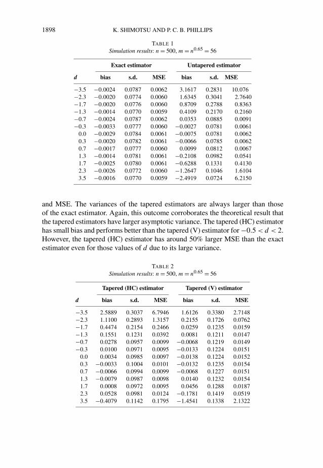
3. Simulations. This section reports some simulations that were conducted toexamine the finite sample performance of the exact LW estimator (hereafter, exactestimator), the LW estimator (hereafter, untapered estimator) and the LW estimatorwith two types of tapering studied by Hurvich and Chen [3] and Velasco [15] withBartlett’s window [hereafter, tapered (HC) and tapered (V) estimator, resp.]. Thetapered (HC) estimator and tapered (V) estimator are consistent and asymptoticallynormal for d ∈ (−0.5,1.5) with limiting variances 1.5/(4m) and 2.1/(4m),respectively (see Remark 1). We generate I (d) processes according to (3) withut ∼ i.i.d.N(0,1). �1 and �2 are set to −6 and 6. Although this setting violatesAssumption 5, it does not appear to adversely affect the performance of theexact estimator. The bias, standard deviation and mean squared error (MSE) werecomputed using 10,000 replications. The sample size and band parameter m werechosen to be n = 500 and m = n0.65 = 56. Values of d were selected in the interval[−3.5,3.5].

Tables 1 and 2 show the simulation results. The exact estimator has littlebias for all values of d . The untapered estimator has a large bias for d > 1,corroborating the theoretical result that it converges to unity in probability [8].When −0.5 < d < 1, the exact and untapered estimators have similar variance


TABLE 1Simulation results: n = 500, m = n0.65 = 56

Exact estimator Untapered estimator

d bias s.d. MSE bias s.d. MSE

−3.5 −0.0024 0.0787 0.0062 3.1617 0.2831 10.076−2.3 −0.0020 0.0774 0.0060 1.6345 0.3041 2.7640−1.7 −0.0020 0.0776 0.0060 0.8709 0.2788 0.8363−1.3 −0.0014 0.0770 0.0059 0.4109 0.2170 0.2160−0.7 −0.0024 0.0787 0.0062 0.0353 0.0885 0.0091−0.3 −0.0033 0.0777 0.0060 −0.0027 0.0781 0.0061

0.0 −0.0029 0.0784 0.0061 −0.0075 0.0781 0.00620.3 −0.0020 0.0782 0.0061 −0.0066 0.0785 0.00620.7 −0.0017 0.0777 0.0060 0.0099 0.0812 0.00671.3 −0.0014 0.0781 0.0061 −0.2108 0.0982 0.05411.7 −0.0025 0.0780 0.0061 −0.6288 0.1331 0.41302.3 −0.0026 0.0772 0.0060 −1.2647 0.1046 1.61043.5 −0.0016 0.0770 0.0059 −2.4919 0.0724 6.2150

and MSE. The variances of the tapered estimators are always larger than thoseof the exact estimator. Again, this outcome corroborates the theoretical result thatthe tapered estimators have larger asymptotic variance. The tapered (HC) estimatorhas small bias and performs better than the tapered (V) estimator for −0.5 < d < 2.However, the tapered (HC) estimator has around 50% larger MSE than the exactestimator even for those values of d due to its large variance.

TABLE 2Simulation results: n = 500, m = n0.65 = 56

Tapered (HC) estimator Tapered (V) estimator

d bias s.d. MSE bias s.d. MSE

−3.5 2.5889 0.3037 6.7946 1.6126 0.3380 2.7148−2.3 1.1100 0.2893 1.3157 0.2155 0.1726 0.0762−1.7 0.4474 0.2154 0.2466 0.0259 0.1235 0.0159−1.3 0.1551 0.1231 0.0392 0.0081 0.1211 0.0147−0.7 0.0278 0.0957 0.0099 −0.0068 0.1219 0.0149−0.3 0.0100 0.0971 0.0095 −0.0133 0.1224 0.0151

0.0 0.0034 0.0985 0.0097 −0.0138 0.1224 0.01520.3 −0.0033 0.1004 0.0101 −0.0132 0.1235 0.01540.7 −0.0066 0.0994 0.0099 −0.0068 0.1227 0.01511.3 −0.0079 0.0987 0.0098 0.0140 0.1232 0.01541.7 0.0008 0.0972 0.0095 0.0456 0.1288 0.01872.3 0.0528 0.0981 0.0124 −0.1781 0.1419 0.05193.5 −0.4079 0.1142 0.1795 −1.4541 0.1338 2.1322


Figures 1 and 2 plot kernel estimates of the densities of the four estimatorsfor the values d = −0.7,0.3,1.3 and 2.3. The sample size and m were chosen asn = 500 and m = n0.65, and 10,000 replications were used. When d = −0.7, theexact and tapered (V) estimators have symmetric distributions centered on −0.7,with the tapered estimator having a flatter distribution. The untapered and tapered(HC) estimators appear to be biased. When d = 0.3, the untapered and exactestimators have almost identical distributions, whereas the two tapered estimatorshave more dispersed distributions. When d = 1.3, the untapered estimator iscentered on unity. In this case, the exact estimator seems to work well, havinga symmetric distribution centered on 1.3. The tapered estimators have flatterdistributions than the exact estimator but otherwise appear reasonable and theyare certainly better than the inconsistent untapered estimator. When d = 2.3, theuntapered and tapered (V) estimators appear centered on 1.0 and 2.0, respectively.In this case, the tapered (HC) estimator is upward biased. Again, the exactestimator has a symmetric distribution centered on the true value 2.3.

In summary, there seems to be little doubt from these results that the exact LWestimator is the best general-purpose estimator over a wide range of d values.

FIG. 1. Densities of the four estimators: n = 500, m = n0.65.


FIG. 2. Densities of the four estimators: n = 500, m = n0.65.

4. Proofs. In this and the following section, |x|+ denotes max{x,1} and x∗denotes the complex conjugate of x. C, c and ε denote generic constants suchthat C,c ∈ (1,∞) and ε ∈ (0,1) unless specified otherwise, and they may takedifferent values in different places.

4.1. Proof of consistency. Define G(d) = G01m

∑m1 λ

2(d−d0)j and S(d) =

R(d) − R(d0). Rewrite S(d) as

S(d) = R(d) − R(d0)

= logG(d)

G(d)− log

G(d0)

G0+ log

(1

m

m∑j=1

j2d−2d0/ m2(d−d0)

2(d − d0) + 1

)

− 2(d − d0)

[1

m

m∑j=1

log j − (logm − 1)

]

+ 2(d − d0) − log(2(d − d0) + 1

).


Define U(d) = 2(d − d0) − log(2(d − d0) + 1) and

T (d) = logG(d0)

G0− log

G(d)

G(d)− log

(1

m

m∑j=1

j2d−2d0/ m2d−2d0

2(d − d0) + 1

)

+ 2(d − d0)

[1

m

m∑j=1

log j − (logm − 1)

],

so that S(d) = U(d) − T (d). For arbitrarily small � > 0, define �1 = {d0 − 12 +

� ≤ d ≤ d0 + 12} and �2 = {d ∈ [�1, d0 − 1

2 + �] ∪ [d0 + 12 ,�2]}, �2 being

possibly empty. Without loss of generality we assume � < 18 hereafter. For

12 > ρ > 0, define Nρ = {d : |d − d0| < ρ}. Then it follows (cf. [11], page 1634)that

Pr(|d − d0| ≥ ρ) ≤ Pr(

infd∈�1\Nρ

S(d) ≤ 0)

+ Pr(

inf�2

S(d) ≤ 0).(9)

Robinson ([11], (3.4), page 1635) shows

infd∈�1\Nρ

U(d) ≥ ρ2/2.(10)

Therefore, Pr(|d − d0| ≥ ρ) → 0 if

sup�1

|T (d)| p→ 0, Pr(

inf�2

S(d) ≤ 0)

→ 0

as n → ∞. From [11], the fourth term of T (d) is O(logm/m) uniformly in d ∈ �1and

sup�1

∣∣∣∣∣2(d − d0) + 1

m

m∑j=1

(j

m

)2d−2d0

− 1

∣∣∣∣∣ = O

(1

m2�

).(11)

Note thatG(d) − G(d)

G(d)

= m−1 ∑m1 λ

2(d−d0)j λ

2(d0−d)j I�dx(λj ) − G0m

−1 ∑m1 λ

2(d−d0)j

G0m−1 ∑m1 λ

2(d−d0)j

= m−1 ∑m1 (j/m)2(d−d0)λ

2(d0−d)j I�dx(λj ) − G0m

−1 ∑m1 (j/m)2(d−d0)

G0m−1 ∑m1 (j/m)2(d−d0)

(12)

= [2(d − d0) + 1]m−1 ∑m1 (j/m)2(d−d0)[λ2(d0−d)

j I�dx(λj ) − G0][2(d − d0) + 1]G0m−1 ∑m

1 (j/m)2(d−d0)

= A(d)

B(d).


Therefore, by the fact that Pr(| logY | ≥ ε) ≤ 2 Pr(|Y − 1| ≥ ε/2) for any

nonnegative random variable Y and ε ≤ 1, sup�1|T (d)| p→ 0 if

sup�1

|A(d)/B(d)| p→ 0.(13)

Define θ = d − d0, and define

Yt (θ) = (1 − L)dXt = (1 − L)d−d0(1 − L)d0Xt = (1 − L)θutI {t ≥ 1}.Hereafter, we use the notation at ∼ I (α) when at is generated by (1) withparameter α. So Yt ∼ I (−θ). Note that

d ∈ �1 ⇐⇒ −12 + � ≤ θ ≤ 1

2 .

Applying Lemma 5.1(a) to (Yt (θ), ut ) and reversing the role of Xt and ut , weobtain

wy(λj ) = wu(λj )Dn(eiλj ; θ) − (2πn)−1/2Uλj n(θ),(14)

and A(d) can be written as, with g = 2(d − d0) + 1,

A(d) = g

m

m∑j=1

(j

m

)2θ

[λ−2θj Iy(λj ) − G0].(15)

Hereafter in this section let Iyj denote Iy(λj ), let wuj denote wu(λj ), and employthe same notation for the other d.f.t.’s and periodograms. From an argument similarto that of [11], page 1636, sup�1

|A(d)| is bounded by

2m−1∑r=1

(r

m

)2� 1

r2 sup�1

∣∣∣∣∣r∑

j=1

[λ−2θj Iyj − G0]

∣∣∣∣∣ + 2

msup�1

∣∣∣∣∣m∑

j=1

[λ−2θj Iyj − G0]

∣∣∣∣∣.(16)

Now

λ−2θj Iyj − G0

= λ−2θj Iyj − λ−2θ

j |Dn(eiλj ; θ)|2Iuj

(17)+ [λ−2θ

j |Dn(eiλj ; θ)|2 − G0/fu(λj )]Iuj

+ [Iuj − |C(eiλj )|2Iεj ]G0/fu(λj ) + G0(2πIεj − 1).

For any η > 0, Lemma 5.2 and Assumption 1 imply that n can be chosen so that∣∣λ−2θj |Dn(e

iλj ; θ)|2 − G0/fu(λj )∣∣ ≤ η + O(λ2

j ) + O(j−1/2),(18)

j = 1, . . . ,m.

The results in [11], page 1637, imply that, uniformly in j = 1, . . . ,m,

E|wuj − C(eiλj )wεj |2 = O(j−1 log(j + 1)

),

(19)E|Iuj − |C(eiλj )|2Iεj | = O

(j−1/2(

log(j + 1))1/2)

.


It follows from (18) and (19) that

m∑r=1

(r

m

)2� 1

r2 sup�1

r∑j=1

∣∣[λ−2θj |Dn(e

iλj ; θ)|2 − G0/fu(λj )]Iuj

+ [Iuj − |C(eiλj )|2Iεj ]G0/fu(λj )∣∣

= Op(η + m2n−2 + m−2� logm).

Robinson ([11], pages 1637–1638) shows∑m

1 (r/m)2�r−2|∑r1(2πIεj − 1)| p→ 0

and m−1 ∑m1 (2πIεj −1)

p→ 0. From (14), the fact that ||A|2 −|B|2| ≤ |A+B||A−B| and the Cauchy–Schwarz inequality we have

E sup�1

∣∣λ−2θj Iyj − λ−2θ

j |Dn(eiλj ; θ)

∣∣2Iuj |

≤(E sup

�1

∣∣∣∣2λ−θj Dn(e

iλj ; θ)wuj − λ−θj

Uλj n(θ)√2πn

∣∣∣∣2)1/2

(20)

×(E sup

�1

∣∣∣∣λ−θj

Uλj n(θ)√2πn

∣∣∣∣2)1/2

.

From (19) and Lemmas 5.2 and 5.3, it follows that, uniformly in j = 1, . . . ,m,

E sup�1

|λ−θj Dn(e

iλj ; θ)wuj |2 = O(1),

E sup�1

∣∣λ−θj (2πn)−1/2Uλj n(θ)

∣∣2 = O(j−1(logn)2)

.

Therefore, we obtain

(20) = O(1 + j−1/2 logn)O(j−1/2 logn) = O(j−1/2(logn)2)

.(21)

It follows that

m−1∑r=1

(r

m

)2� 1

r2 E sup�1

∣∣∣∣∣r∑

j=1

[λ−2θj Iyj − λ−2θ

j |Dn(eiλj ; θ)|2Iuj ]

∣∣∣∣∣= O

(m−�(logn)2)

,

and hence the first term in (16) is op(1). Using the same technique, we can show

that the second term in (16) is op(1), and sup�1|A(d)| p→ 0 follows. Equation (11)

gives sup�1|B(d) − G0| = O(m−2�), and (13) follows.


Now we take care of �2 = {d ∈ [�1, d0 − 12 + �] ∪ [d0 + 1

2 ,�2]} = {θ ∈[�1 − d0,−1

2 + �] ∪ [12 ,�2 − d0]} to show Pr(inf�2 S(d) ≤ 0) → 0. Note that

S(d) = log G(d) − log G(d0) − 2(d − d0)1

m

m∑j=1

logλj

= log1

m

m∑j=1

I�dxj − log1

m

m∑j=1

I�d0xj

− 2(d − d0) log2π

n− 2(d − d0)

1

m

m∑j=1

log j

= log1

m

m∑j=1

λ2(d−d0)j λ

2(d0−d)j I�dxj − log

1

m

m∑j=1

I�d0xj

− 2(d − d0) log2π

n− 2(d − d0) logp

= log1

m

m∑j=1

(j

p

)2θ

λ−2θj I�dxj − log

1

m

m∑j=1

I�d0xj

= log D(d) − log D(d0),

where p = exp(m−1 ∑m1 log j) ∼ m/e as m → ∞. Applying (17) with θ = 0 and

proceeding similarly to the argument below (17), we obtain

log D(d0) − logG0 = log

(1 + G−1

0

(1

m

m∑j=1

Iuj − G0

))= op(1).

Therefore, Pr(inf�2 S(d) ≤ 0) tends to 0 if there exists δ > 0 such that

Pr(

inf�2

log D(d) − logG0 ≤ log(1 + δ)

)= Pr

(inf�2

D(d) − G0 ≤ δG0

)→ 0

as n → 0. Now, for any fixed κ ∈ (0,1) we have

D(d) = 1

m

m∑j=1

(j

p

)2θ

λ−2θj Iyj ≥ 1

m

m∑j=[κm]

(j

p

)2θ

λ−2θj Iyj .

Let∑′ denote the sum over j = [κm], . . . ,m. It follows that, for d ∈ �2,

D(d) − G0

(22) ≥ m−1′∑

(j/p)2θ (λ−2θj Iyj − G0) + G0

(m−1

′∑(j/p)2θ − 1

).


From Lemma 5.5, by choosing δ first and then κ sufficiently small, for large m wehave

inf�2

G0

(m−1

′∑(j/p)2θ − 1

)> 4δG0.

Therefore, Pr(inf�2 S(d) ≤ 0) → 0 if there exists δ > 0 such that

Pr

(inf�2

(m−1

′∑(j/p)2θ (λ−2θ

j Iyj − G0)

)≤ −3δG0

)→ 0(23)

as n → ∞. We proceed to show (23) for subsets of �2.First we consider �1

2 = {θ ∈ [−12 ,−1

2 + �]}. Rewrite

m−1′∑

(j/p)2θ (λ−2θj Iyj − G0) = �1n(θ) + �2n(θ),

where

�1n(θ) = m−1′∑

(j/p)2θ [λ−2θj Iyj − λ−2θ

j |Dn(eiλj ; θ)|2Iuj ],(24)

�2n(θ) = m−1′∑

(j/p)2θ [λ−2θj |Dn(e

iλj ; θ)|2Iuj − G0].(25)

For �1n(θ), since (20) and (21) are still valid for θ ∈ �12, we have

E sup�1

2



∣∣ = O(j−1/2(logn)2)

,

and it follows from Lemma 5.4 that E sup�12|�1n(θ)| = o(1). For �2n(θ), rewrite

�2n(θ) as

m−1′∑

(j/p)2θ [λ−2θj |Dn(e

iλj ; θ)|2 − G0/fu(λj )]Iuj(26)

+ m−1′∑

(j/p)2θ [Iuj − |C(eiλj )|2Iεj ]G0/fu(λj )(27)

+ m−1′∑

(j/p)2θG0(2πIεj − 1).(28)

sup�12|(26)|, sup�1

2|(27)| = op(1) follows from (19) and Lemmas 5.2(b) and 5.4.

For (28), summation by parts gives

(28) = G0

(m

p

)2θ 1

m

m−1∑r=[κm]

((r

m

)2θ

−(

r + 1

m

)2θ) r∑j=[κm]

(2πIεj − 1)

+ G0

(m

p

)2θ 1

m

m∑j=[κm]

(2πIεj − 1)

= I (θ) + II(θ).


As in [11], page 1637, write

2πIεj − 1 = 1

n

n∑t=1

(ε2t − 1) + 1

n

∑∑s �=t

cos{(s − t)λj }εsεt ,

from which it follows that

sup�1

2

|I (θ)| ≤ C

m

m∑r=[κm]

∣∣∣∣ sup�1

2

(r

m

)2θ ∣∣∣∣∣∣∣∣∣1

n

n∑t=1

(ε2t − 1)

∣∣∣∣∣+ C

m

m∑r=[κm]

∣∣∣∣ sup�1

2

(r

m

)2θ ∣∣∣∣ 1

rn

∣∣∣∣∣∑∑s �=t

r∑j=[κm]

cos{(s − t)λj }εsεt

∣∣∣∣∣.From [11], (3.19) and (3.20), we have n−1 ∑n

1(ε2t − 1)

p→ 0 and

E

(∑∑s �=t

εsεt

r∑j=[κm]

cos{(s − t)λj })2

= O(rn2).

In conjunction with max[κm]≤r≤m sup�2(r/m)2θ = O(1), we obtain sup�1

2|I (θ)| =

op(1). sup�12|II(θ)| = op(1) follows from a similar argument. Hence

sup�12|(28)| = op(1) and sup�1

2|�2n(θ)| = op(1) follow, and we have estab-

lished (23) for θ ∈ �12.

For �22 = {θ : 1

2 ≤ θ ≤ 32} define Zn(θ) = ∑n

t=1 Yt (θ) ∼ I (1 − θ) with 1 − θ ∈[−1

2 , 12 ]. From Lemma 5.1(b) we have

wyj = (1 − eiλj )wzj + (2πn)−1/2eiλj Zn(θ).(29)

DefineDnj (θ) = λ−θ

j (1 − eiλj )Dn(eiλj ; θ − 1),

Unj (θ) = λ−θj (1 − eiλj )(2πn)−1/2Uλj n(θ − 1),

and then applying (14) to (Zt (θ), ut ) gives

λ−θj wyj = Dnj (θ)wuj − Unj (θ) + λ−θ

j (2πn)−1/2eiλj Zn(θ).(30)

Since θ − 1 ≥ −12 , from Lemma 5.2 we have, for θ ∈ �2

2,

Dnj (θ) = e−(π/2)θi + O(λj ) + O(j−1/2) uniformly in θ.(31)

With a slight abuse of notation, rewrite

m−1′∑

(j/p)2θ (λ−2θj Iyj − G0)

= m−1′∑

(j/p)2θ [λ−2θj Iyj − |Dnj (θ)|2Iuj ]

(32)

+ m−1′∑

(j/p)2θ [|Dnj (θ)|2Iuj − G0]= �1n(θ) + �2n(θ).


Therefore, (23) follows if, for θ ∈ �22,

Pr(

infθ

�1n(θ) ≤ −2δG0

)→ 0, sup

θ

|�2n(θ)| = op(1) as n → ∞.(33)

supθ |�2n(θ)| = op(1) follows straightforwardly from (31) and by the sameargument as the one for θ ∈ �1

2. For �1n(θ), substituting (30) to the definitionof �1n(θ) gives

�1n(θ) = m−1′∑

(j/p)2θ |Unj (θ)|2(34)

+ m−1′∑

(j/p)2θλ−2θj (2πn)−1Z2

n(35)

− 2 Re

[m−1

′∑(j/p)2θDnj (θ)∗w∗

ujUnj (θ)

](36)

− 2 Re

[m−1

′∑(j/p)2θ Unj (θ)λ−θ

j (2πn)−1/2eiλj Zn(θ)

](37)

+ 2 Re

[m−1


ujλ−θj (2πn)−1/2eiλj Zn(θ)

].(38)

Equation (34) is almost surely nonnegative. Lemma 5.3 gives

E supθ

|Unj (θ)|2 = O(j−1(logn)2)

,(39)

and hence supθ |(36)| = op(1) follows from (39) and Lemma 5.4. Therefore,(33) and hence (23) follow if, for any ζ > 0,

Pr(

infθ

[(35) + (37) + (38)] ≤ −ζ

)→ 0 as n → ∞.(40)

We proceed to show (40). First, there exists η > 0 such that, uniformly in θ ,

(35) = p−2θ (2π)−2θ−1n2θ−1Zn(θ)2m−1′∑

1 ≥ η(m−θnθ−1/2Zn(θ)

)2.

From (39) and Lemma 5.4, we have, uniformly in θ ,

(37) = m−θnθ−1/2Zn(θ) · Op(m−1/2 logn).

For (38), it follows from (31), eiλj = 1 + O(λj ) and Lemmas 5.4 and 5.6 that

m−1′∑

(j/p)2θDnj (θ)∗w∗ujλ

−θj (2πn)−1/2eiλj Zn(θ)

= (2πn)−1/2Zn(θ)e(π/2)θim−1′∑

(j/p)2θw∗ujλ

−θj

(41)

+ (2πn)−1/2Zn(θ)m−1′∑

(j/p)2θw∗ujλ

−θj [O(λj ) + O(j−1/2)]

= m−θnθ−1/2Zn(θ)[Op(m−1/2 logm) + Op(mn−1)].


Therefore, we can write

(37) + (38) = m−θnθ−1/2Zn(θ) · Rn(θ,ω),(42)

where ω denotes an element of the sample space �, and

supθ

|Rn(θ,ω)| = Op(kn), kn = m−1/2 logn + mn−1 → 0.(43)

Before showing (40), define

�1 = {(ω, θ) ∈ � × � :m−θnθ−1/2|Zn(θ)| < kn logm},�2 = {(ω, θ) ∈ � × � :m−θnθ−1/2|Zn(θ)| ≥ kn logm},

where � is the domain of θ (�12 in this case), so that �1 ∪ �2 = � × �. Then{

(ω, θ) :η(m−θnθ−1/2Zn(θ)

)2 − |m−θnθ−1/2Zn(θ) · Rn(θ,ω)| ≤ −ζ}

= {(ω, θ) :

(η(m−θnθ−1/2Zn(θ)

)2

− |m−θnθ−1/2Zn(θ) · Rn(θ,ω)| ≤ −ζ) ∩ �1

}∪ {

(ω, θ) :(η(m−θnθ−1/2Zn(θ)

)2

− |m−θnθ−1/2Zn(θ) · Rn(θ,ω)| ≤ −ζ) ∩ �2

}⊆ {

(ω, θ) :η(m−θnθ−1/2Zn(θ)

)2 − kn logm|Rn(θ,ω)| ≤ −ζ}

∪ {(ω, θ) :m−θnθ−1/2|Zn(θ)|[ηkn logm − |Rn(θ,ω)|] ≤ −ζ }⊆ {(ω, θ) :kn logm|Rn(θ,ω)| ≥ ζ } ∪ {(ω, θ) :ηkn logm − |Rn(θ,ω)| ≤ 0}.

Therefore,{ω : inf

θ

[η(m−θnθ−1/2Zn(θ)

)2 − |m−θnθ−1/2Zn(θ) · Rn(θ,ω)|] ≤ −ζ

}⊆

{ω : sup

θ

kn logm|Rn(θ,ω)| ≥ δG0

}

∪{ω :ηkn logm − sup

θ

|Rn(θ,ω)| ≤ 0},

and it follows that

Pr(

infθ

[η(m−θnθ−1/2Zn(θ)

)2 − |m−θnθ−1/2Zn · Rn(θ,ω)|] ≤ −ζ

)≤ Pr

(kn logm sup

θ

|Rn(θ,ω)| ≥ ζ

)

+ Pr(ηkn logm − sup

θ

|Rn(θ,ω)| ≤ 0)

→ 0,


because supθ |Rn(θ,ω)| = Op(kn), and k2n logm → 0 from Assumption 4. There-

fore (40) follows, and hence (23) holds for θ ∈ �22.

For �32 = {θ :−3

2 ≤ θ ≤ −12}, from Lemma 5.1 we have

wyj = (1 − eiλj )−1w�yj − (1 − eiλj )−1(2πn)−1/2eiλj Yn(θ),(44)

where �Yt(θ) ∼ I (−θ − 1). With a slight abuse of notation, define

Dnj (θ) = λ−θj (1 − eiλj )−1Dn(e

iλj ; θ + 1),

Unj (θ) = λ−θj (1 − eiλj )−1(2πn)−1/2Uλj n(θ + 1).

Then, applying (14) to (�Yt(θ), ut ) gives

λ−θj wyj = Dnj (θ)wuj − Unj (θ) + λ−θ

j (2πn)−1/2eiλj (1 − eiλj )−1Yn(θ).(45)

Dnj (θ) and Unj (θ) satisfy (31) and (39) for θ ∈ �32, because −θ − 1 ∈ [−1

2 , 12 ].

Using the decomposition (32) and the same argument as the one for θ ∈ �22, we

obtain

m−1′∑


= m−1′∑

(j/p)2θ [λ−2θj Iyj − |Dnj (θ)|2Iuj ] + op(1),

where op(1) is uniform in θ ∈ �32. Using (45), rewrite the first term on the right-

hand side as

m−1′∑

(j/p)2θ |Unj (θ)|2(46)

+ m−1′∑

(j/p)2θλ−2θj (2πn)−1|1 − eiλj |−2Yn(θ)2(47)

− 2 Re

[m−1


ujUnj (θ)

](48)

− 2 Re

[m−1

′∑(j/p)2θ Unj (θ)λ−θ

j (2πn)−1/2eiλj (1 − eiλj )−1Yn(θ)

](49)

+ 2 Re

[m−1

′∑(j/p)2θDnj (θ)∗

(50)

× w∗ujλ

−θj (2πn)−1/2eiλj (1 − eiλj )−1Yn(θ)

].

Equation (46) is almost surely nonnegative. Because Dnj (θ) and Unj (θ) satisfy(31) and (39), it follows from a decomposition similar to (41) and Lemmas


5.4 and 5.6 that supθ |(48)| = op(1) and (49) + (50) = m−θ−1nθ+1/2Yn(θ) ×Op(m−1/2 logn + mn−1). Finally, (47) is equal to

p−2θn2θ−1(2π)−2θ−1m−1′∑ |1 − eiλj |−2Yn(θ)2

= p−2θn2θ−1(2π)−2θ−1Yn(θ)2m−1′∑

λ−2j

(1 + o(1)

)(51)

≥ ηm−2θ−2n2θ+1Yn(θ)2,

for some η > 0. Therefore we can apply the argument following (42) with slightchanges to show (23) for θ ∈ �3

2.For �4

2 = {θ : 32 ≤ θ ≤ 5

2}, by applying (29) twice and (14), we obtain

λ−θj wyj = Dnj (θ)wuj − Unj (θ)

+ λ−θj (2πn)−1/2eiλj

[(1 − eiλj )

n∑t=1

Zt(θ) + Zn(θ)

],

where

Dnj (θ) = λ−θj (1 − eiλj )2Dn(e

iλj ; θ − 2),

Unj (θ) = λ−θj (1 − eiλj )2(2πn)−1/2Uλj n(θ − 2),

and Dnj (θ) and Unj (θ) satisfy (31) and (39). We proceed to evaluate the terms inm−1 ∑′(j/p)2θλ−2θ

j Iyj . First, observe that

m−1′∑

(j/p)2θλ−2θj (2πn)−1

∣∣∣∣∣(1 − eiλj )

n∑t=1

Zt(θ) + Zn(θ)

∣∣∣∣∣2

(52)

= p−2θn2θ−1(2π)−2θ−1m−1′∑∣∣∣∣∣(1 − eiλj )

n∑t=1

Zt(θ) + Zn(θ)

∣∣∣∣∣2

.

By applying Lemma 5.10(a) with Q3 = Q2 = 0, Q1 = ∑n1 Zt(θ) and Q0 = Zn(θ),

there exists η > 0 such that, for sufficiently large n,

(52) ≥ ηm−2θ+2n2θ−3

(n∑

t=1

Zt(θ)

)2

+ ηm−2θn2θ−1Zn(θ)2 = �3n(θ)

uniformly in θ . Of the other terms in m−1 ∑′(j/p)2θλ−2θj Iyj , the terms involving

the cross products of wuj , Unj (θ) and (1 − eiλj )∑n

1 Zt(θ) + Zn(θ) are dominated


by �3n(θ). For instance, proceeding as in (41) gives

m−1′∑

(j/p)2θDnj (θ)wujλ−θj (2πn)−1/2e−iλj

[(1 − e−iλj )

n∑t=1

Zt(θ) + Zn(θ)

]

= m−θ+1nθ−3/2n∑

t=1

Zt(θ) · Op(m−1/2 logn + n−1m)

+ m−θnθ−1/2Zn(θ) · Op(m−1/2 logn + n−1m),

where the Op(·) terms are uniform in θ . Therefore, the terms in m−1 ∑′(j/p)2θ ×[λ−2θ

j Iyj −|Dnj (θ)|2Iuj ] are either op(1) or nonnegative or dominated by �3n(θ).

We obtain supθ |m−1 ∑′(j/p)2θ [|Dnj (θ)|2Iuj − G0]| = op(1) by using (31) andproceeding as in (26)–(28) and the following argument, and thus (23) follows forθ ∈ �4

2.Since |θ | ≤ �2 − �1 ≤ 9

2 , the proof is completed by showing (23) for theremaining subsets of �2 :

�52 = {

θ :−52 ≤ θ ≤ −3

2

},

�62 = {

θ : 72 ≤ θ ≤ 5

2

},

�72 = {

θ :−72 ≤ θ ≤ −5

2

},

�82 = {

θ : 92 ≤ θ ≤ 7

2

},

�92 = {

θ :−92 ≤ θ ≤ −7

2

}.

Applying (29) or (44) repeatedly and (14) gives the required result for �·2. For

instance, for �92 = {θ :−9

2 ≤ θ ≤ −72}, applying (44) four times and then (14), we

have

λ−θj wyj = Dnj (θ)wuj − Unj (θ) − λ−θ

j (2πn)−1/2eiλj Wnj ,

where

Dnj (θ) = λ−θj (1 − eiλj )−4Dn(e

iλj ; θ + 4),

Unj (θ) = λ−θj (1 − eiλj )−4(2πn)−1/2Uλj n(θ + 4),

Wnj = (1 − eiλj )−4�3Yn(θ) − (1 − eiλj )−3�2Yn(θ)

− (1 − eiλj )−2�Yn(θ) − (1 − eiλj )−1Yn(θ),

and Dnj (θ) and Unj (θ) satisfy (31) and (39). We can easily obtain

m−1′∑


= m−1′∑

(j/p)2θ [λ−2θj Iyj − |Dnj (θ)|2Iuj ] + op(1),


where op(1) is uniform in θ ∈ �92. For the first term on the right-hand side, from

Lemma 5.10(b) we have, for large n and η > 0,

m−1′∑

(j/p)2θλ−2θj (2πn)−1|Wnj |2

= (2π)−2θ−1n2θ−1p−2θm−1′∑ |Wnj |2(53)

≥ ηn2θ−1m−2θ

[m−8n8(

�3Yn(θ))2 + m−6n6(

�2Yn(θ))2

+m−4n4(�Yn(θ)

)2 + m−2n2Yn(θ)2

],

uniformly in θ . The terms involving the cross products between wuj , Unj (θ)

and Wnj are dominated by (53). The other terms in m−1 ∑′(j/p)2θ [λ−2θj Iyj −

|Dnj (θ)|2Iuj ] are either op(1) or almost surely nonnegative, and hence (23)follows.

4.2. Proof of asymptotic normality. Theorem 2.1 holds under the currentconditions and implies that with probability approaching 1, as n → ∞ d satisfies

0 = R′(d) = R′(d0) + R′′(d)(d − d0),(54)

where |d − d0| ≤ |d − d0|. From the fact that

∂

∂dw�dxj = ∂

∂d

1√2πn

n∑t=1

eiλj t (1 − L)dXt

= 1√2πn

n∑t=1

eiλj t log(1 − L)(1 − L)dXt ,

∂2

∂d2 w�dxj = 1√2πn

n∑t=1

eiλj t (log(1 − L))2

(1 − L)dXt ,

we obtain

R′′(d) = G2(d)G(d) − G21(d)

G2(d)= G2(d)G0(d) − G2

1(d)

G20(d)

,

where

G1(d) = 1

m

m∑j=1

∂

∂d

[w�dxjw

∗�dxj

] = 1

m

m∑j=1

2 Re[wlog(1−L)�dxjw

∗�dxj

],

G2(d) = 1

m

m∑j=1

∂2

∂d2

[w�dxjw

∗�dxj

] = 1

m

m∑j=1

Wx(L,d, j),


Wx(L,d, j) = 2 Re[w(log(1−L))2�dxjw

∗�dxj

] + 2Ilog(1−L)�dxj ,

G0(d) = 1

m

m∑j=1

j2θλ−2θj Iyj ,

G1(d) = 1

m

m∑j=1

j2θλ−2θj 2 Re

[wlog(1−L)yjw

∗yj

],

G2(d) = 1

m

m∑j=1

j2θλ−2θj Wy(L,0, j),

and θ = d − d0 and Yt (θ) = (1 − L)dXt = (1 − L)θutI {t ≥ 1}, as defined in theproof of Theorem 2.1. Fix ε > 0 and let M = {d : (logn)4|d − d0| < ε}. From (9)in the proof of Theorem 2.1 we have

Pr(d /∈ M) ≤(

inf�1\M

S(d) ≤ 0)

+ o(1).

Hence, in view of (10), Pr(d /∈ M) tends to zero if

sup�1

|A(d)/B(d)| = op

((logn)−8)

,(55)

where A(d) and B(d) are defined in (12) in the proof of Theorem 2.1. FromAssumption 1′, (18) is strengthened to∣∣λ−2θ

j |Dn(eiλj ; θ)|2 − G0/fu(λj )

∣∣ = O(λβj ) + O(j−1/2),

(56)j = 1, . . . ,m.

Therefore, proceeding as in the proof of Theorem 2.1, we obtain

m∑r=1

(r

m

)2� 1

r2 sup�1

∣∣∣∣∣r∑

j=1

[λ−2θj Iyj − 2πG0Iεj ]

∣∣∣∣∣ = Op

(mβn−β + m−�(logn)2)

.

Robinson ([11], (4.9), page 1643) shows

r∑j=1

(2πIεj − 1) = Op(r1/2) as n → ∞ for 1 ≤ r ≤ m,(57)

and it follows that∑m

1 (r/m)2�r−2|∑r1(2πIεj − 1)| = O(m−2� logm). Applying

the same argument to the second term of (16), we obtain sup�1|A(d)| =

op((logn)−8), and (55) follows in view of (11). Thus we assume d ∈ M in thefollowing discussion of Gk(d).


Now we derive the approximation of Gk(d) for k = 0,1,2. For G0(d) observethat

E supθ∈M

|λ−2θj Iyj − Iuj |

≤ E supθ∈M



∣∣(58)

+ E supθ∈M

∣∣λ−2θj |Dn(e

iλj ; θ)|2 − 1∣∣Iuj

= O(j−1/2(logn)2 + j2n−2)

, j = 1, . . . ,m,

where the third line follows from (21) and Lemma 5.2. Since |j2θ − 1|/|2θ | ≤(log j)n2|θ | ≤ (log j)n1/ logn = e log j on M , we have

supM

|j2θ − 1| = O((logn)−3)

,

(59)supM

|j2θ | = O(1), j = 1, . . . ,m.

Therefore, in view of (58) and EIuj = O(1) [following from (19)], we obtain

supM

∣∣∣∣∣G0(d) − 1

m

m∑j=1

Iuj

∣∣∣∣∣≤ sup

M

∣∣∣∣∣ 1

m

m∑j=1

j2θ [λ−2θj Iyj − Iuj ]

∣∣∣∣∣ + supM

∣∣∣∣∣ 1

m

m∑j=1

(j2θ − 1)Iuj

∣∣∣∣∣= op

((logn)−2)

.

For G1(d), from (14) and Lemma 5.9 we have

λ−2θj wlog(1−L)yjw

∗yj + Jn(e

iλj )Iuj

= Jn(eiλj )[1 − λ−2θ

j |Dn(eiλj ; θ)|2]Iuj

− Jn(eiλj )λ−θ

j Dn(eiλj ; θ)wuj · λ−θ

j (2πn)−1/2Uλj n(θ)∗

− λ−θj Dn(e

iλj ; θ)∗w∗uj · λ−θ

j (2πn)−1/2Vnj (θ)

− λ−2θj (2πn)−1Uλj n(θ)∗Vnj (θ).

Then, since Jn(eiλj ) = O(logn), it follows from (59) and Lemmas 5.2, 5.3 and 5.9

that

1

m

m∑j=1

supM

j2θ∣∣ Re

[λ−2θ

j wlog(1−L)yjw∗yj + Jn(e

iλj )Iuj

]∣∣ = op

((logn)−1)

.


In conjunction with (59), Jn(eiλj ) = O(logn) and EIuj = O(1), it follows that

supM

∣∣∣∣∣G1(d) + 1

m

m∑j=1

2 Re[Jn(eiλj )]Iuj

∣∣∣∣∣= sup

M

∣∣∣∣∣ 1

m

m∑j=1

(1 − j2θ )2 Re[Jn(eiλj )]Iuj

∣∣∣∣∣ + op

((logn)−1)

= op

((logn)−1)

.

For G2(d), the same line of argument as above with Lemma 5.9(c) gives

supM

∣∣∣∣∣G2(d) − 1

m

m∑j=1

{2 Re[Jn(eiλj )2] + 2Jn(e

iλj )Jn(eiλj )∗}Iuj

∣∣∣∣∣= sup

M

∣∣∣∣∣G2(d) − 1

m

m∑j=1

4{Re[Jn(eiλj )]}2Iuj

∣∣∣∣∣= op(1).

From (19) and Assumption 1′, we obtain

E|Iuj − G0Iεj | ≤ E|Iuj − |C(eiλj )|2Iεj | + E2π |fu(λj ) − fu(0)|Iεj

= O(j−1/2(

log(j + 1)) + jβn−β)

, j = 1, . . . ,m.

Therefore, in view of Jn(eiλj ) = O(logn), EIεj = 1, and Cov(Iεj , Iεk) = O(1) if

j = k and O(n−1) if j �= k, we have

G0(d) = m−1m∑

j=1

Iuj + op

((logn)−2)

= G0m−1

m∑j=1

Iεj + op

((logn)−2)

= G0 + op

((logn)−2)

,

G1(d) = −2m−1m∑

j=1

Re[Jn(eiλj )]Iuj + op

((logn)−1)

= −G0m−1

m∑j=1

2 Re[Jn(eiλj )]Iεj + op

((logn)−1)

= −G0m−1

m∑j=1

2 Re[Jn(eiλj )] + op

((logn)−1)


and

G2(d) = m−1m∑

j=1

4{Re[Jn(eiλj )]}2Iuj + op(1)

= G0m−1

m∑j=1

4{Re[Jn(eiλj )]}2Iεj + op(1)

= G0m−1

m∑j=1

4{Re[Jn(eiλj )]}2 + op(1).

It follows that

R′′(d) = [G2(d)G0(d) − G21(

d)][G0(d)]−2

= G20m

−1 ∑m1 4{Re[Jn(e

iλj )]}2 − {G0m−1 ∑m

1 2 Re[Jn(eiλj )]}2 + op(1)

{G0 + op((logn)−2)}2(60)

= 4m−1m∑

j=1

{Re[Jn(eiλj )]}2 − 4

{m−1

m∑j=1

Re[Jn(eiλj )]

}2

+ op(1).

From Lemma 5.8(a) and a routine calculation, we obtain

m−1m∑

j=1

{Re[Jn(eiλj )]}2 = m−1

m∑j=1

(logλj )2 + o(1),

{m−1

m∑j=1

Re[Jn(eiλj )]

}2

=(m−1

m∑j=1

logλj

)2

+ o(1).

Therefore, 14 times (60) is, apart from op(1) terms,

m−1m∑

j=1

(logλj )2 −

(m−1

m∑j=1

logλj

)2

= m−1m∑

j=1

(log j)2 −(m−1

m∑j=1

log j

)2

→ 1,

and R′′(d) = 4 + op(1) follows.Now we find the limit distribution of m1/2R′(d0). In view of Lemma 5.9(b),

E|wuj − C(eiλj )wεj |2 = O(j−1 log(j + 1)) [see (19)] and E|Jnλj(eiλj L)εn|2 =

O(nj−1) [see (77)], we obtain

−wlog(1−L)ujw∗uj

= [Jn(eiλj )wuj + rnj ]w∗

uj


− C(1)(2πn)−1/2Jnλj(e−iλj L)εnC(eiλj )∗w∗

εj

− C(1)(2πn)−1/2Jnλj(e−iλj L)εn[w∗

uj − C(eiλj )∗w∗εj ]

= Jn(eiλj )Iuj − C(1)(2πn)−1/2Jnλj

(e−iλj L)εnC(eiλj )∗w∗εj + Rnj ,

where rnj is defined in Lemma 5.9(b), and E|j1/2Rnj | = o(1) + O(j−1/2 logm)

as n → ∞. It follows that m1/2G1(d0) is equal to

−m−1/2m∑

j=1

2 Re[Jn(eiλj )]Iuj(61)

+ C(1)m−1/2m∑

j=1

2 Re[(2πn)−1/2Jnλj

(e−iλj L)εnC(eiλj )∗w∗εj

](62)

+ op(1) + Op

(m−1/2(logm)2)

.

From Lemma 5.8(a) we have

(61) = 2m−1/2m∑

j=1

(logλj )Iuj + Op(m5/2n−2) + Op(m−1/2 logm).

For (62), in view of the fact that

w∗εj = (2πn)−1/2

n∑p=1

e−ipλj εp = (2πn)−1/2n−1∑q=0

eiqλj εn−q,

we obtain the decomposition

m−1/2m∑

j=1

(2πn)−1/2Jnλj(e−iλj L)εnC(eiλj )∗w∗

εj

(63)

= m−1/2m∑

j=1

C(eiλj )∗(2πn)−1

(n−1∑p=0

jλjpe−ipλj εn−p

)(n−1∑q=0

eiqλj εn−q

).

Because the εt are martingale differences, the second moment of (63) is boundedby

1

mn2

m∑j=1

m∑k=1

n−1∑p=0

∣∣jλjp

∣∣∣∣jλkp

∣∣ + 2

mn2

m∑j=1

m∑k=1

n−1∑p=0

∣∣jλjp

∣∣ n−1∑r=0

∣∣j−λkr

∣∣(64)

+ 1

mn2

m∑j=1

m∑k=1

n−1∑p=0,p �=q

∣∣jλjp

∣∣∣∣j−λkp

∣∣∣∣∣∣∣n−1∑q=0

eiq(λj−λk)

∣∣∣∣∣.(65)


Since jλjp = O(max{|p|−1+ nj−1, logn}) from Lemma 5.8, (64) is bounded by

1

mn2

m∑j=1

m∑k=1

[n−1∑p=0

(logn)2 +n−1∑p=0

n

j |p|+n−1∑r=0

n

k|r|+

]

= O(mn−1(logn)2 + m−1(logn)4)

,

and, in view of the fact that∑n−1

q=0 eiq(λj−λk) = nI {j = k}, (65) is bounded by

1

mn

m∑j=1

n−1∑p=0

∣∣jλjp

∣∣2 = O

(1

mn

m∑j=1

n−1∑p=0

j−1|p|−1+ n logn

)= O

(m−1(logn)3)

,

giving (62) = op(1). Therefore, we obtain

m1/2G1(d0) = 2m−1/2m∑

j=1

(logλj )Iuj + op(1).

Let νj = logλj − m−1 ∑m1 logλj = log j − m−1 ∑m

1 log j with∑m

1 νj = 0. Thenit follows that

m1/2R′(d0) = m1/2

[G1(d0)

G(d0)− 2

1

m

m∑j=1

logλj

]

= 2m−1/2 ∑m1 (logλj )Iuj + op(1) − (m−1 ∑m

1 logλj )2m−1/2 ∑m1 Iuj

m−1 ∑m1 Iuj

= 2m−1/2 ∑m1 νj Iuj + op(1)

G0 + op(1)

= 2m−1/2 ∑m1 νj (Iuj − G0) + op(1)

G0 + op(1)

= 2m−1/2 ∑m1 νj (2πIεj − 1) + op(1)

1 + op(1)

d→ N(0,4),

where the fifth line follows from [11], page 1644, completing the proof.

5. Technical lemmas. Lemma 5.2 extends Lemma A.3 of Phillips andShimotsu [8] to hold uniformly in θ . Its proof follows easily from the proof ofLemmas A.2 and A.3 of [8] and is therefore omitted.

LEMMA 5.1 ([7], Theorem 2.2). (a) If Xt follows (1), then

wu(λ) = Dn(eiλ;d)wx(λ) − (2πn)−1/2einλXλn(d),


where Dn(eiλ;d) = ∑n

k=0(−d)k

k! eikλ and

Xλn(d) = Dnλ(e−iλL;d)Xn =

n−1∑p=0

dλpe−ipλXn−p, dλp =n∑

k=p+1

(−d)k

k! eikλ.

(b) If Xt follows (1) with d = 1, then

wx(λ)(1 − eiλ) = wu(λ) − (2πn)−1/2ei(n+1)λXn.

LEMMA 5.2 (cf. [8], Lemmas A.2 and A.3). (a) Uniformly in θ ∈ [−C,C]and in j = 1,2, . . . ,m with m = o(n), as n → ∞,

λ−θj (1 − eiλj )θ = e−(π/2)θi + O(λj ), λ−2θ

j |1 − eiλj |2θ = 1 + O(λ2j ).

(b) Uniformly in θ ∈ [−1 + ε,C] and in j = 1,2, . . . ,m with m = o(n), asn → ∞,

λ−θj Dn(e

iλj ; θ) = e−(π/2)θi + O(λj ) + O(j−1−θ ),

λ−2θj |Dn(e

iλj ; θ)|2 = 1 + O(λ2j ) + O(j−1−θ ).

LEMMA 5.3. Let Uλn(θ) = Dnλ(e−iλL; θ)un = ∑n−1

p=0 θλpe−ipλun−p . Underthe assumptions of Theorem 2.1, we have, uniformly in j = 1, . . . ,m, as n → ∞,

E supθ∈[−1/2,1/2]

∣∣nθ−1/2j1/2−θ Uλj n(θ)∣∣2 = O

((logn)2)

.

PROOF. When θ = 0, the result follows immediately because Uλj n(0) = 0.

When θ �= 0, define ap = θλjpe−ipλj so that Uλj n(θ) = ∑n−1p=0 apun−p . We

suppress the dependence of ap on θ and λj . Summation by parts gives

Uλj n(θ) =n−2∑p=0

(ap − ap+1)

p∑q=0

un−q + an−1

n−1∑q=0

un−q.

Phillips and Shimotsu ([8], page 670) show that (note that Phillips and Shimotsuuse λs instead of λj to denote Fourier frequencies)

ap − ap+1 = bnp(θ) + (−θ)n

n! e−ipλj ,

where

bnp(θ) =n−1∑

k=p+1

(1 + θ)�(k − θ)

�(−θ)�(k + 2)ei(k−p)λj .(66)


Then, since an−1 = (−θ)ne−i(n−1)λj /n!, we have

Uλj n(θ) =n−2∑p=0

bnp(θ)

p∑q=0

un−q

+ (−θ)n

n!n−2∑p=0

e−ipλj

p∑q=0

un−q + (−θ)n

n! e−i(n−1)λj

n−1∑q=0

un−q

(67)

=n−2∑p=0

bnp(θ)

p∑q=0

un−q + (−θ)n

n!n−1∑p=0

e−ipλj

p∑q=0

un−q

= U1n(θ) + U2n(θ).

We proceed to show that the elements of nθ−1/2j1/2−θU·n(θ) are of the statedorder. First, for U1n, we have

supθ

|nθ−1/2j1/2−θU1n(θ)| ≤n−2∑p=0

supθ

|nθ−1/2j1/2−θbnp(θ)|∣∣∣∣∣

p∑q=0

un−q

∣∣∣∣∣.Because

∑∞−∞ Eutut+q = 2πfu(0) = 2πG0 < ∞, it follows from Kronecker’slemma that, uniformly in p = 0, . . . , n − 1,

E

( p∑q=0

un−q

)2

= (p + 1)

p∑q=−p

(1 − |q|/(p + 1)

)Eutut+q = O(|p|+).(68)

Therefore, if we have, uniformly in p = 0, . . . , n − 1 and j = 1, . . . ,m,

supθ∈[−1/2,1/2]

|nθ−1/2j1/2−θbnp(θ)| = O(|p|−3/2+ ),(69)

it follows from Minkowski’s inequality that

E supθ

|nθ−1/2j1/2−θU1n(θ)|2 = O

((n−2∑p=0

|p|−1+

)2)= O

((logn)2)

.(70)

To show (69), Phillips and Shimotsu ([8], page 670, equation (21)) show that

|bnp(θ)| = O(min{|p|−θ−1+ , |p|−θ−2+ nj−1})(71)

uniformly in θ ∈ [−12 , 1

2 ], p = 0, . . . , n − 1, and j = 1, . . . ,m. Although Phillipsand Shimotsu do not state explicitly that the bound (71) holds uniformly inθ ∈ [−1

2 , 12 ], it is clear from its proof that (71) holds uniformly in θ ∈ [−1

2 , 12 ].

Then (69) follows from (71) because

0 ≤ p ≤ n/j :nθ−1/2j1/2−θ |p|−θ−1+ = (j |p|+/n)1/2−θ |p|−3/2+ ≤ |p|−3/2

+ ,

n/j ≤ p ≤ n :nθ−1/2j1/2−θp−θ−2nj−1 = (jp/n)−θ−1/2p−3/2 ≤ p−3/2.


For U2n = ((−θ)n/n!)∑n−10 e−ipλj

∑p0 un−q , first we rewrite the sum as

n−1∑p=0

e−ipλj

p∑q=0

un−q =n∑

n−p=1

ei(n−p)λj

n∑n−q=n−p

un−q

=n∑

k=1

uk

k∑q=1

eiqλj

(72)

=n∑

k=1

uk

eiλj (1 − eikλj )

1 − eiλj

= eiλj

1 − eiλj

n∑k=1

uk − eiλj

1 − eiλj(2πn)1/2wu(λj ).

Since (−θ)n/n! = O(n−θ−1) uniformly in θ ∈ [−12 , 1

2 ] and (1 − eiλj )−1 =O(nj−1), E supθ |nθ−1/2j1/2−θU2n|2= O(1) follows from (68) and E|wu(λj )|2 =O(1) ([11], page 1637). �

LEMMA 5.4. For κ ∈ (0,1) and C ∈ (1,∞), as m → ∞,

(a) sup−C≤γ≤C

∣∣∣∣∣ 1

m

m∑j=[κm]

(j

m

)γ

−∫ 1

κxγ dx

∣∣∣∣∣ = O(m−1),

(b) sup−C≤γ≤C

∣∣∣∣∣m−1m∑

j=[κm](j/m)γ

∣∣∣∣∣ = O(1),

lim infm→∞ inf−C≤γ≤C

(m−1

m∑j=[κm]

(j/m)γ

)> ε > 0.

PROOF. Note that [κm] ≥ 3 for large m. For part (a), since

1

m

m∑j=[κm]

(j

m

)γ

=m∑

j=[κm]

∫ j/m

(j−1)/m

(j

m

)γ

dx,

∫ 1

κxγ dx =

m∑j=[κm]

∫ j/m

(j−1)/mxγ dx −

∫ κ

([κm]−1)/mxγ dx,

their difference is bounded uniformly in γ by, for sufficiently large m:m∑

j=[κm]

∣∣∣∣ ∫ j/m

(j−1)/m

{(j

m

)γ

− xγ

}dx

∣∣∣∣ + ∫ κ

κ−(2/m)xγ dx

≤ c

m2

m∑j=[κm]

(j

m

)−C−1

+ c

m= O(m−1),


by the mean value theorem. Part (b) follows immediately from part (a). �

LEMMA 5.5. For p ∼ m/e as m → ∞ and � ∈ (0, 12e

), there exist ε ∈ (0,0.1)

and κ ∈ (0, 14) such that, for all fixed κ ∈ (0, κ] and sufficiently large m:

(a) inf−C≤γ≤−1+2�

1

m

m∑j=[κm]

(j

p

)γ

≥ 1 + 2ε,

(b) inf1≤γ≤C

1

m

m∑j=[κm]

(j

p

)γ

≥ 1 + 2ε.

PROOF. From Lemma 5.4 we obtain, for large m,

inf−C≤γ≤−1+2�

1

m

m∑j=[κm]

(j

p

)γ

≥ inf−C≤γ≤−1+2�

1

m

p∑j=[κm]

(j

p

)γ

≥ 1

m

p∑j=[κm]

(j

p

)−1+2�

∼ 1

e

∫ 1

κex2�−1 dx = 1 − (κe)2�

2�e,

inf1≤γ≤C

1

m

m∑j=[κm]

(j

p

)γ

∼ inf1≤γ≤C

eγ

γ + 1(1 − κγ+1) ≥ e

2(1 − κ2),

where the last inequality holds because eγ /(γ + 1) is monotone increasing forγ ≥ 1. Since 2�e < 1, choosing κ sufficiently small gives the stated results. �

LEMMA 5.6. For κ ∈ (0,1), C ∈ (1,∞) and m = o(n), as n → ∞,

E supα∈[−C,C]

∣∣∣∣∣ 1

m

m∑j=[κm]

(j

m

)α

wu(λj )

∣∣∣∣∣ = O(m−1/2 logm).

PROOF. Summation by parts gives

1

m

m∑j=[κm]

(j

m

)α

wu(λj )

= 1

m

m−1∑r=[κm]

[(r

m

)α

−(

r + 1

m

)α] r∑j=[κm]

wu(λj ) + 1

m

m∑j=[κm]

wu(λj ).

Note that, uniformly in r = 1, . . . ,m − 1 and α,∣∣∣∣( r

m

)α

−(

r + 1

m

)α∣∣∣∣ =(

r

m

)α∣∣∣∣1 −(

1 + 1

r

)α∣∣∣∣ ≤ c

(r

m

)−C 1

r,(73)


because supα |(1+x)α −1| ≤ C2Cx for 0 ≤ x ≤ 1. The results in ([11], page 1637)imply that E|wu(λj ) − C(eiλj )wε(λj )|2 = O(j−1 log(j + 1)) uniformly in j =1, . . . ,m, giving

E

∣∣∣∣∣r∑

j=[κm]wu(λj )

∣∣∣∣∣2

= O(r log(r + 1)

), r = [κm], . . . ,m.(74)

From (73), (74) and Lemma 5.4, E supα∈[−C,C] |m−1 ∑m[κm](j/m)αwu(λj )| isbounded by

m−1m−1∑

r=[κm](r/m)−Cr−1/2 log r + m−1/2 logm = O(m−1/2 logm),

giving the required result. �

LEMMA 5.7. Define Jn(L) = ∑nk=1 Lk/k and Dn(L;d) = ∑n

k=0(−d)k

k! Lk .Then:

(a) Jn(L) = Jn(eiλ) + Jnλ(e

−iλL)(e−iλL − 1),

(b) Jn(L)Dn(L;d) = Jn(eiλ)Dn(e

iλ;d) + Dn(eiλ;d)Jnλ(e

−iλL)(e−iλL − 1)

+Jn(L)Dnλ(e−iλL;d)(e−iλL − 1),

where

Jnλ(e−iλL) =

n−1∑p=0

jλpe−ipλLp, jλp =n∑

p+1

1

keikλ,

Dnλ(e−iλL;d) =

n−1∑p=0

dλpe−ipλLp, dλp =n∑

p+1

(−d)k

k! eikλ.

PROOF. For part (a) see [9], formula (32). For part (b), from Lemma 2.1 of [7]we have Dn(L;d) = Dn(e

iλ;d)+Dnλ(e−iλL;d)(e−iλL−1), and the stated result

follows immediately. �

LEMMA 5.8. Let Jn(eiλ) = ∑n

k=1 eikλ/k and jλp = ∑nk=p+1 eikλ/k, as

defined in Lemma 5.7. Then uniformly in p = 0, . . . , n − 1 and j = 1, . . . ,m withm = o(n), as n → ∞:

(a) Jn(eiλj ) = − logλj + i

2(π − λj ) + O(λ2

j ) + O(j−1),

(b) jλjp = O(min{|p|−1+ nj−1, logn}).PROOF. For (a), first we have

Jn(eiλj ) =

n∑k=1

1

keikλj =

∞∑k=1

1

keikλj −

∞∑k=n+1

1

keikλj .(75)


The first term on the right-hand side of (75) is equal to ([16], page 5)

∞∑k=1

cos kλj

k+ i

∞∑k=1

sinkλj

k= − log

∣∣∣∣2 sinλj

2

∣∣∣∣ + i1

2(π − λj ).

Since 2 sin(λj/2) = λj + O(λ3j ) = λj (1 + O(λ2

j )), the right-hand side is equal to

− logλj − log(1 + O(λ2

j )) + i

1

2(π − λj )

= − logλj + O(λ2j ) + i

2(π − λj ).

For the second term on the right-hand side of (75), summation by parts gives∣∣∣∣∣∞∑

k=n+1

1

keikλj

∣∣∣∣∣=

∣∣∣∣∣ limN→∞

[n+N−1∑r=n+1

(1

r− 1

r + 1

) r∑k=n+1

eikλj + 1

n + N

n+N∑k=n+1

eikλj

]∣∣∣∣∣≤ C

(nj−1

∞∑k=n

r−2 + j−1

)= O(j−1),

giving (a). Part (b) follows from the fact that

|jλjp| ≤ (p + 1)−1 maxp+1≤N≤n

∣∣∣∣∣N∑

k=p+1

eikλj

∣∣∣∣∣ and jλjp = O

(n∑

k=0

|k|−1+

).

�

LEMMA 5.9. Suppose Yt = (1 − L)θutI {t ≥ 1} . Under the assumptions ofTheorem 2.2 we have:

(a) −wlog(1−L)y(λj ) = Jn(eiλj )Dn(e

iλj ; θ)wu(λj ) + n−1/2Vnj (θ),

(b) −wlog(1−L)u(λj ) = Jn(eiλj )wu(λj )

− C(1)(2πn)−1/2Jnλj(e−iλj L)εn + rnj ,

(c) w(log(1−L))2y(λj ) = Jn(eiλj )2Dn(e

iλj ; θ)wu(λj ) + n−1/2�nj (θ),

where, uniformly in j = 1, . . . ,m, as n → ∞,

E supθ

|nθ−1/2j1/2−θVnj (θ)|2 = O((logn)4)

,

E|j1/2rnj |2 = o(1) + O(j−1),

E supθ

|nθ−1/2j1/2−θ�nj (θ)|2 = O((logn)6)

.


PROOF. Define ut = utI {t ≥ 1}, so that Yt = Dt−1(L; θ)ut = Dn(L; θ)ut fort ≤ n. Since Yt = 0 for t ≤ 0, we have

log(1 − L)Yt = (−L − L2/2 − L3/3 − · · ·)Yt = −Jn(L)Yt .

For parts (a) and (b), from Lemma 5.7(b) we have

− log(1 − L)Yt

= Jn(L)Dn(L; θ)ut

= Jn(eiλj )Dn(e

iλj ; θ)ut + Dn(eiλj ; θ)Jnλj

(e−iλj L)(e−iλj L − 1)ut

+ Jn(L)Dnλj(e−iλj L; θ)(e−iλj L − 1)ut .

Since∑n

t=1 eitλj (e−iλj L − 1)ut = −un, taking the d.f.t. of the right-hand sidegives

Jn(eiλj )Dn(e

iλj ; θ)wu(λj ) − (2πn)−1/2Dn(eiλj ; θ)Jnλj

(e−iλj L)un

(76)− (2πn)−1/2Jn(L)Dnλj

(e−iλj L; θ)un.

Note that Lemma 5.2(b) gives |Dn(eiλj ; θ)| ≤ cλθ

j . Therefore part (a) follows if

E∣∣Jnλj

(e−iλj L)un

∣∣2 = O(nj−1),(77)

E supθ

∣∣nθ−1/2j1/2−θJn(L)Dnλj(e−iλj L; θ)un

∣∣2 = O((logn)4)

.(78)

First we show (77). Define a′p = jλjpe−ipλj = ∑n

k=p+1 k−1ei(k−p)λj , so that

Jnλj(e−iλj L)un = ∑n−1

p=0 a′pun−p = ∑n−1

p=0 a′pun−p . Then summation by parts

gives

Jnλj(e−iλj L)un =

n−2∑p=0

(a′p − a′

p+1)

p∑q=0

un−q + a′n−1

n−1∑q=0

un−q.

Observe that

a′p − a′

p+1 =n∑

k=p+1

1

kei(k−p)λj −

n∑k=p+2

1

kei(k−p−1)λj

=n−1∑

k=p+1

[1

k− 1

k + 1

]ei(k−p)λj + 1

ne−ipλj

=n−1∑

k=p+1

1

k(k + 1)ei(k−p)λj + 1

ne−ipλj .


Define cnp = ∑n−1k=p+1

1k(k+1)

ei(k−p)λj . Then since a′n−1 = n−1e−i(n−1)λj , we

obtain

Jnλj(e−iλj L)un

=n−2∑p=0

cnp

p∑q=0

un−q + 1

n

n−2∑p=0

e−ipλj

p∑q=0

un−q + 1

ne−i(n−1)λj

n−1∑q=0

un−q

=n−2∑p=0

cnp

p∑q=0

un−q + 1

n

n−1∑p=0

e−ipλj

p∑q=0

un−q(79)

=n−2∑p=0

cnp

p∑q=0

un−q +[

1

n

eiλj

1 − eiλj

n∑k=1

uk − 1

n

eiλj

1 − eiλj(2πn)1/2wu(λj )

]

= J1n + J2n,

where the fourth line follows from (72). E|J2n|2 = O(nj−2) in view of the orderof magnitude of E|∑n

1 uk|2 and E|wu(λj )|2. For J1n, since

|cnp| =∣∣∣∣∣

n−1∑k=p+1

1

k(k + 1)ei(k−p)λj

∣∣∣∣∣≤ |p|−2+ max

1≤N≤n

∣∣∣∣∣p+N∑p+1

eikλj

∣∣∣∣∣ ≤ C|p|−2+ nj−1,

|cnp| ≤∣∣∣∣∣

n−1∑k=p+1

1

k(k + 1)

∣∣∣∣∣ ≤ C|p|−1+ ,

we have

|cnp| ≤ C min{|p|−1+ , |p|−2+ nj−1}.(80)

Therefore, it follows from (68) and Minkowski’s inequality that

E|J1n|2 = O

(( n/j∑p=0

|p|−1/2+ +

n∑p=n/j

n

j|p|−3/2

+

)2)= O(nj−1),(81)

and hence (77) follows.Now we move to the proof of (78). When θ = 0, then Dnλj

(e−iλj L; θ) = 0,and (78) follows immediately. Assume θ �= 0. If we have, uniformly in r =0,1, . . . ,

E supθ

|nθ−1/2j1/2−θLrDnλj(e−iλj L; θ)un|2 = O

((logn)2)

,(82)


then (78) follows because Minkowski’s inequality gives

E supθ

∣∣nθ−1/2j1/2−θJn(L)Dnλj(e−iλj L; θ)un

∣∣2≤ E

(n−1∑p=1

p−1 supθ

∣∣nθ−1/2j1/2−θLpDnλj(e−iλj L; θ)un

∣∣)2

≤(

n−1∑p=1

p−1(E sup

θ

∣∣nθ−1/2j1/2−θLpDnλj(e−iλj L; θ)un

∣∣2)1/2)2

= O((logn)4)

.

We proceed to show (82). For r ≥ n, (82) follows immediately becauseLrDnλj

(e−iλj L; θ)un = 0. For r = 0, . . . , n − 1, using a decomposition similarto (67) gives

LrDnλj(e−iλj L; θ)un

=n−2∑p=0

bnp(θ)Lrp∑

q=0

un−q + (−θ)n

n! Lrn−1∑p=0

e−ipλj

p∑q=0

un−q

= U ′1n(θ) + U ′

2n(θ),

where bnp(θ) is defined in (66). For U ′1n(θ), since E(Lr ∑p

q=0un−q)2 = O(|p|1/2

+ ),

the arguments in the proof of Lemma 5.3 go through and E supθ |nθ−1/2j1/2−θ ×U ′

1n(θ)|2 = O((logn)2) holds. For U ′2n(θ), using a decomposition similar to (72)

gives

U ′2n(θ) = (−θ)n

n!eiλj

1 − eiλjLr

n∑k=1

uk − (−θ)n

n!eiλj

1 − eiλjLr

n∑k=1

eikλjuk

= (−θ)n

n!eiλj

1 − eiλj

n−r∑k=1

uk − (−θ)n

n!eiλj

1 − eiλjeirλj

n−r∑q=1

eiqλj uq.

Since E(∑n−r

k=1 uk)2 = O(n1/2) for any r , E supθ |nθ−1/2j1/2−θU ′

2n(θ)|2 = O(1)

and (82) follow if, for m = o(n),

max1≤r≤n

max1≤j≤m

E

∣∣∣∣∣(2πr)−1/2r∑

k=1

eikλj uk

∣∣∣∣∣2

= O(1).(83)

We establish (83) to complete the proof of part (a). An elementary calculationgives

E

∣∣∣∣∣(2πr)−1/2r∑

k=1

eikλj uk

∣∣∣∣∣2

=∫ π

−πfu(λ)Kr(λ − λj ) dλ,


where Kr(λ) = (2πr)−1∑rs=1

∑rt=1 ei(t−s)λ is Fejér’s kernel. From Zygmund [16],

pages 88–90,∫ π−π |Kr(λ)|dλ < A and |Kr(λ)| ≤ Ar−1λ−2 for a finite con-

stant A. Furthermore, from Assumption 1 there exists η ∈ (0, π) such thatsupλ∈[−η,η] |fu(λ)| < C, and inf|λ|>η |λ − λj | ≥ η/2 if λj < η/2. It follows thatfor sufficiently large n∫ π

−πfu(λ)Kr(λ − λj ) dλ

=∫|λ|≤η

fu(λ)Kr(λ − λj ) dλ +∫η≤|λ|≤π

fu(λ)Kr(λ − λj ) dλ

≤ AC + Ar−1(η/2)−2∫η≤|λ|≤π

fu(λ) dλ < ∞,

uniformly in j = 1, . . . ,m, and (83) follows.For part (b), in view of (76), Dn(e

iλj ;0) = 1 and Dnλj(e−iλj L;0) = 0, part (b)

follows if, as n → ∞, uniformly in j = 1, . . . ,m,

E∣∣j1/2n−1/2Jnλj

(e−iλj L)(un − C(1)εn

)∣∣2 = o(1) + O(j−1).(84)

Using the same decomposition as (79), write j1/2n−1/2Jnλj(e−iλj L)(un −

C(1)εn) asn−2∑p=0

j1/2√

ncnp

p∑q=0

(un−q − C(1)εn−q

)(85)

+ j1/2

n√

n

eiλj

1 − eiλj

n∑k=1

(un−k − C(1)εn−k

)(86)

− j1/2

n

eiλj√

2π

1 − eiλj[wu(λj ) − C(1)wε(λj )].

If we have

E

[ p∑q=0


)]2

(87)

={

O(|p|+), uniformly in p = 0, . . . , n − 1,o(p), as p → ∞,

then it follows from Minkowski’s inequality and the order of cnp given by (80) that

(E|(85)|2)1/2 = O

((j/n)1/2

√n/j∑

p=0

|p|−1/2+

)

+ o

((j/n)1/2

n/j∑p=√

n/j

p−1/2 + (j/n)1/2n∑

p=n/j

n

jp−3/2

)


= O((j/n)1/4) + o(1)

= o(1),

because√

n/j ≥ √n/m → ∞ from Assumption 4′. To prove (87), note that when

p = 0, (87) follows immediately. When p ≥ 1, observe that

E

[ p∑q=0


)]2

≤ 2E

[ p∑q=0

un−q

]2

+ 2E

[C(1)

p∑q=0

εn−q

]2

.

Since the first term on the right-hand side is uniformly O(p) from (68) and thesecond term on the right-hand side is equal to 2C(1)2(p + 1), the first part of (87)holds. For the second part of (87), note that the left-hand side of (87) is equal to(γq = Eutut+q )

p∑r=−p

(p + 1 − |r|)γr − 2C(1)

p∑q=0

q∑r=0

cq−r + (p + 1)C(1)2

= −(p + 1)∑

|r|≥p+1

γr − 2p∑

r=1

rγr + 2C(1)(p + 1)∑

r≥p+1

cr − 2C(1)

p∑r=1

rcr .

If∑∞−∞ ar converges, then

∑|r|≥p+1 ar tends to 0 as p → ∞; thus the first and

third terms are o(p) because both∑∞−∞ γr and

∑∞−∞ cr converge. The secondand fourth terms are o(p) from Kronecker’s lemma, and the second part of (87)follows. Obviously E|(86)|2 = O(j−1), and (84) follows.

For part (c), first from Lemma 2.1 of [7] and Lemma 5.7 we have

Jn(L)2 = Jn(L)[Jn(eiλ) + Jnλ(e

−iλL)(e−iλL − 1)]= Jn(L)Jn(e

iλ) + Jn(L)Jnλ(e−iλL)(e−iλL − 1)

= Jn(eiλ)2 + Jn(e

iλ)Jnλ(e−iλL)(e−iλL − 1)

+ Jn(L)Jnλ(e−iλL)(e−iλL − 1),

Dn(L; θ) = Dn(eiλ; θ) + Dnλ(e

−iλL; θ)(e−iλL − 1).

It follows that(log(1 − L)

)2Yt = Jn(L)2Dn(L; θ)ut

= Jn(eiλ)2Dn(e

iλ; θ)ut

+ Dn(eiλ; θ)[Jn(e

iλ) + Jn(L)]Jnλ(e−iλL)(e−iλL − 1)ut

+ Jn(L)2Dnλ(e−iλL; θ)(e−iλL − 1)ut .


Taking its d.f.t. gives

Jn(eiλj )2Dn(e

iλj ; θ)wu(λj )

− (2πn)−1/2Dn(eiλj ; θ)[Jn(e

iλj ) + Jn(L)]Jnλj(e−iλj L)un

− (2πn)−1/2Jn(L)2Dnλs (e−iλj L; θ)un.

By the same argument as the ones used in showing (77) and (82), we obtain

E∣∣LqJnλj

(e−iλj L)un

∣∣2 = O(nj−1), q = 0,1, . . . .

In conjunction with Jn(eiλj ) = O(logn), Minkowski’s inequality and (82), it

follows that

E supθ

∣∣nθ−1/2j1/2−θDn(eiλj ; θ)[Jn(e

iλj ) + Jn(L)]Jnλj(e−iλj L)un

∣∣2= O

((logn)2)

,

E supθ

∣∣nθ−1/2j1/2−θJn(L)2Dnλj(e−iλj L; θ)un

∣∣2= O

((logn)6)

for j = 1, . . . ,m, giving the stated result. �

LEMMA 5.10. Let Qk , k = 0, . . . ,3, be any real numbers, κ ∈ (0, 18), and

1/m + m/n → 0 as n → ∞. Then there exists η > 0 not depending on Qk suchthat, for sufficiently large n:

(a) m−1m∑

j=[κm]|(1 − eiλj )3Q3 + (1 − eiλj )2Q2 + (1 − eiλj )Q1 + Q0|2

≥ η(m6n−6Q23 + m4n−4Q2

2 + m2n−2Q21 + Q2

0),

(b) m−1m∑

j=[κm]|(1 − eiλj )−1Q3 + (1 − eiλj )−2Q2

+ (1 − eiλj )−3Q1 + (1 − eiλj )−4Q0|2≥ η(m−2n2Q2

3 + m−4n4Q22 + m−6n6Q2

1 + m−8n8Q20).

PROOF. Define

A(λ) = (1 − eiλ)3Q3 + (1 − eiλ)2Q2 + (1 − eiλ)Q1 + Q0.

Since 1 − eiλ = −iλ + O(λ2) as λ → 0, we have

A(λ) = iλ3Q3 − λ2Q2 − iλQ1 + Q0(88)

+ O(λ4)Q3 + O(λ3)Q2 + O(λ2)Q1.


Applying 2|a||b| ≤ |a|2 + |b|2 to the product terms involving the remainder terms,we obtain

|A(λ)|2 = (λ2Q2 − Q0)2 + (λ3Q3 − λQ1)

2 + R(λ),(89)

where R(λ) = O(λ7)Q23 + O(λ5)Q2

2 + O(λ3)Q21 + O(λ)Q2

0. First we show that

m−1m∑

j=[κm](λ2

jQ2 − Q0)2 ≥ η(m4n−4Q2

2 + Q20).(90)

When sgn(Q2) �= sgn(Q0), then (90) holds from Lemma 5.4. When sgn(Q2) =sgn(Q0), without loss of generality assume Q2,Q0 > 0. Note that λ2

jQ2 is

an increasing function of j . Now suppose (λm/2)2Q2 − Q0 ≥ 0. Then, since

(λ3m/4)2 = 9

4(λm/2)2, we have, for j = 3m/4, . . . ,m,

λ2jQ2 − Q0 ≥ 9

4(λm/2)2Q2 − Q0

= 14(λm/2)

2Q2 + 2(λm/2)2Q2 − Q0

≥ 14(λm/2)

2Q2 + Q0.

Now suppose (λm/2)2Q2 −Q0 < 0. Then, since (λm/4)

2 = 14(λm/2)

2, we have, forj = 1, . . . ,m/4,

λ2jQ2 − Q0 ≤ 1

4(λm/2)2Q2 − Q0

= −14(λm/2)

2Q2 + [12(λm/2)

2Q2 − Q0]

≤ −14(λm/2)

2Q2 − 12Q0.

Therefore, either for j = 1, . . . ,m/4 or for j = 3m/4, . . . ,m, we have

|λ2jQ2 − Q0| ≥ 1

4(λm/2)2Q2 + 1

2Q0(91)

and (90) follows immediately. The same argument gives, if sgn(Q3) = sgn(Q1),

|λ3jQ3 − λjQ1| ≥ λj

{14(λm/2)

2|Q3| + 12 |Q1|},(92)

either for j = 1, . . . ,m/4 or for j = 3m/4, . . . ,m, and it follows from (91) and(92) that

m−1m∑

j=[κm](λ3

jQ3 − λjQ1)2 ≥ η(m6n−6Q2

3 + m2n−2Q21).

For R(λ) in (89), it follows from Lemma 5.4 that

m−1m∑

j=[κm]R(λj )

= O(m7n−7)Q23 + O(m5n−5)Q2

2 + O(m3n−3)Q21 + O(mn−1)Q2

0,


and part (a) follows. For part (b), rewrite the term inside the summation as

|(1 − eiλj )−4A(λj )|2 = ∣∣λ−4j

(1 + O(λj )

)A(λj )

∣∣2.Applying (88) and the following argument with (91) and (92) gives part (b). �

Acknowledgments. The authors thank an Associate Editor and three refereesfor helpful comments and advice that led to a substantial revision of the originalversion of this paper. K. Shimotsu thanks the Cowles Foundation for hospitalityduring his stay from January 2002 to August 2003. Simulations were performedin MATLAB.

REFERENCES

[1] GEWEKE, J. and PORTER-HUDAK, S. (1983). The estimation and application of long memorytime series models. J. Time Ser. Anal. 4 221–238.

[2] HENRY, M. and ROBINSON, P. M. (1996). Bandwidth choice in Gaussian semiparametricestimation of long range dependence. Athens Conference on Applied Probability and TimeSeries. Lecture Notes in Statist. 115 220–232. Springer, New York.

[3] HURVICH, C. M. and CHEN, W. W. (2000). An efficient taper for potentially overdifferencedlong-memory time series. J. Time Ser. Anal. 21 155–180.

[4] KIM, C. S. and PHILLIPS, P. C. B. (1999). Log periodogram regression: The nonstationarycase. Mimeographed, Cowles Foundation, Yale Univ.

[5] KÜNSCH, H. (1987). Statistical aspects of self-similar processes. In Proc. First World Congressof the Bernoulli Society (Yu. Prokhorov and V. V. Sazanov, eds.) 1 67–74. VNU SciencePress, Utrecht.

[6] MARINUCCI, D. and ROBINSON, P. M. (1999). Alternative forms of fractional Brownianmotion. J. Statist. Plann. Inference 80 111–122.

[7] PHILLIPS, P. C. B. (1999). Discrete Fourier transforms of fractional processes. CowlesFoundation Discussion Paper #1243, Yale Univ. Available at cowles.econ.yale.edu.

[8] PHILLIPS, P. C. B. and SHIMOTSU, K. (2004). Local Whittle estimation in nonstationary andunit root cases. Ann. Statist. 32 656–692.

[9] PHILLIPS, P. C. B. and SOLO, V. (1992). Asymptotics for linear processes. Ann. Statist. 20971–1001.

[10] ROBINSON, P. M. (1995). Log-periodogram regression of time series with long-rangedependence. Ann. Statist. 23 1048–1072.

[11] ROBINSON, P. M. (1995). Gaussian semiparametric estimation of long-range dependence. Ann.Statist. 23 1630–1661.

[12] ROBINSON, P. M. (2005). The distance between rival nonstationary fractional processes.J. Econometrics. To appear.

[13] ROBINSON, P. M. and MARINUCCI, D. (2001). Narrow-band analysis of nonstationaryprocesses. Ann. Statist. 29 947–986.

[14] SHIMOTSU, K. (2004). Exact local Whittle estimation of fractional integration with unknownmean and time trend. Mimeographed, Queen’s Univ., Kingston.


[15] VELASCO, C. (1999). Gaussian semiparametric estimation of non-stationary time series.J. Time Ser. Anal. 20 87–127.

[16] ZYGMUND, A. (1977). Trigonometric Series. Cambridge Univ. Press.

DEPARTMENT OF ECONOMICS

QUEEN’S UNIVERSITY

KINGSTON, ONTARIO

CANADA K7L 3N6E-MAIL: [email protected]

COWLES FOUNDATION FOR

RESEARCH IN ECONOMICS

YALE UNIVERSITY

P.O. BOX 208281NEW HAVEN, CONNECTICUT 06520-8281USAE-MAIL: [email protected]

exact local whittle estimation of fractional …korora.econ.yale.edu/phillips/pubs/art/p1156.pdf ·...

Documents