exact tuning of pid controllers in control feedback design
TRANSCRIPT
Exact Tuning of PID Controllers
in Control Feedback Design∗
Lorenzo Ntogramatzidis† Augusto Ferrante★
†Department of Mathematics and Statistics,
Curtin University, Perth WA 6845, Australia.
E-mail: [email protected].
★Dipartimento di Ingegneria dell’Informazione,
Universita di Padova, via Gradenigo, 6/B – I-35131 Padova, Italy.
E-mail: [email protected]
Abstract
In this paper, we introduce a range of techniques for the exact design of PID controllers for feedback
control problems involving requirements on the steady-state performance and standard frequency domain
specifications on the stability margins and crossover frequencies. These techniques hinge on a set of simple
closed-form formulae for the explicit computation of the parameters of the controller in finite terms as func-
tions of the specifications, and therefore they eliminate the need for graphical, heuristic or trial-and-error
procedures. The relevance of this approach isi) theoretical, since a closed-form solution is provided for the
design of PID-type controllers with standard frequency domain specifications;ii) computational, since the
techniques presented here are readily implementable as software routines, for example using MATLABR⃝;
iii) educational, because the synthesis of the controller reduces to a simple exercise on complex numbers
that can be solved with pen, paper and a scientific calculator. These techniques also appear to be very conve-
nient within the context of adaptive control and self-tuning strategies, where the controller parameters have
to be calculated on-line. Furthermore, they can be easily combined with graphical and first/second order
plant approximation methods in the cases where the model of the system to be controlled is not known.
1 Introduction
Countless tuning methods have been proposed for PID controllers over the last seventy years. Accounting
for all of them goes beyond the possibilities of this paper. We limit ourselves tonoticing that many surveys
and textbooks have been entirely devoted to these techniques, that differfrom each other in terms of the
∗This work was partially supported by the Australian Research Council (Discovery Grant DP0986577) and by the Italian Ministry
for Education and Resarch (MIUR) under PRIN grant “Identification and Robust Control of Industrial Systems”.
specifications, the amount of knowledge on the model of the plant and in termsof tools exploited, see e.g.
[2, 3, 4, 13] and the references therein.
Recently, renewed interest has been devoted to design techniques for PID controllers under frequency
domain specifications, see e.g. [16, 12, 9, 8, 7]. In particular, much effort has been devoted to the computation
of the parameters of the PID controllers that guarantee desired values ofthe gain/phase margins and of the
crossover frequency. Specifications on the stability margins have always been extensively utilised in feedback
control system design to ensure a robust control system. It is also commonto encounter specifications on
phase margin and gain crossover frequency, since these two parameters together often serve as a performance
measure of the control system. Indeed, loosely speaking, the phase margin is related to characteristics of the
response such as the peak overshoot and the resonant peak, while the gain crossover frequency is related to the
rise time and the bandwidth, [6, 5].
In the last fifteen years, three important sets of techniques have been proposed to deal with requirements
on the phase/gain margins and on the gain crossover frequency, to the end of avoiding the trial-and-error nature
of classical control methods based on Bode and Nichols diagrams. The first one is a graphical method hinging
on design charts, and exploits an interpolation technique to determine the parameters of the PID controller.
This method can be adapted to control problems involving different kinds ofcompensators, including phase-
correction networks, and can deal with specification on the stability margins,crossover frequencies and on
the steady-state performance, [16]. A second important set of techniques that can handle specifications on the
phase and gain margins relies on the approximation of the plants dynamics with a first (or second) order plus
delay model, [7], [12]. A third numerical technique has been recently proposed in [9] in which the objective is
the determination of the set of PID controllers that satisfy given requirements on the gain and phase margins,
but without the flexibility required to also deal with specifications on the crossover frequencies and on the
steady-state performance.
To overcome the difficulties and approximations of trial-and-error procedures on Bode and Nyquist plots,
and of the three above described design methods, a unified design framework is presented in this paper for
the closed-form solution of the feedback control problem with PID controllers. The problem of determin-
ing closed-form expressions for the parameters of the controller to exactly meet the aforementioned design
specifications has been described as a difficult one, [7], and this in part explains the popularity of heuristic,
numerical and graphical solutions to this problem, [6], [11]. In this paper, we show that this is not the case:
simple closed-form formulae are easily established for the computation of the parameters of a PID controller
thatexactlymeets specifications on the steady-state performance, stability margins and crossover frequencies,
without the need to resort to approximations for the transfer function of theplant.
There are several advantages connected with the use of the methods presented here for the synthesis of
PID controllers:i) unlike other analytical synthesis methods [14], steady-state performancespecifications can
be handled easily; Moreover, the desired phase/gain margins and crossover frequency can be achieved exactly,
without the need for trial-and-error, approximations of the plant dynamicsor graphical considerations;ii) a
closed-form solution to the feedback control problem allows to analyse how the solution changes as a result
of variations of the problem data; Moreover, the explicit formulae presented here can be exploited for the
self-tuning of the controller;iii) very neat necessary and sufficient solvability conditions can be derived for
each controller and each set of specifications considered, and reliablemethods can be established to select
the compensator structure to be employed depending on the specifications imposed; iv) Several important
questions arising in the design of PID controllers can find a precise answer for the first time. For example,
is it possible to determine in finite terms the range of phase margins that can be achieved at a particular gain
crossover frequency for each type of compensator belonging to the family of PID controllers?v) The approach
presented here can be used jointly with graphical considerations on Bodeor Nichols diagrams to determine the
set of solutions of the control problem in the case of inequality constraints;vi) The formulae presented here
are straightforwardly implementable as MATLABR⃝ routines. Furthermore, as shown in the several numerical
examples throughout the paper, the calculation of the parameters of the controller is carried out via standard
manipulations on complex numbers, and therefore appears to be very suitable for educational purposes;vii)
The generality of this method allows more complex compensator structures to be taken into account, as well.
For example, the proper versions of the PID and PD controllers will be considered as well;viii) In the case
of additional degrees of freedom in the solution of the control problem, it ispossible to exactly establish how
to select the parameters to be chosen in order to guarantee the solvability of the problem;ix) The closed-form
formulae that deliver the parameters of the PID controller as a function of the specifications only depend on
the magnitude and argument of the frequency response of the system to becontrolled at the desired crossover
frequency. As such, this method can be used in conjunction with a graphical method based onany of the
standard diagrams for the representation of the dynamics of the frequency response, e.g., the Bode, Nyquist or
Nichols diagrams;x) In the case a mathematical model of the plant or a graphic representation of itsfrequency
reponse are not available, the technique presented in this paper can be used on a first/second order plus delay
approximation of the plant. The extra flexibility offered by the design method presented here consists in the
fact that the formulae for the computation of the parameters are not linked to aparticular structure of the
plant. This means that, differently from other approaches based on suchapproximation, when a more accurate
mathematical model is available for the model of the plant, the formulae presentedhere can still be used
without modifications, and will deliver more reliable values for the parametersof the compensator.
This paper provides a unified and comprehensive exposition of this technique, not only for PID controllers
in standard form, but also for PI and PD controllers, as well as for modified (bi-)proper PID and PD controllers
with approximation of the derivative action. The basic problem consideredthroughout the paper consists in
finding the parameters of the controller that guarantees a certain phase margin and crossover frequency, and
to satisfy appropriate steady-state requirements. Standard PID controllers will be considered first. Differently
from the synthesis with lead and lag networks [1], [15], here it is necessary to distinguish between two different
types of steady-state requirements. In fact, due to the pole at the origin in thetransfer function of the standard
PID controller, it is essential to discriminate between the case where the steady-state specifications impose a
constraint on the Bode gain (or integral constant) of the PID controller, and the case where the presence of
the pole at the origin in the PID controller alone is sufficient to satisfy the steady-state requirements. The
synthesis procedures differ significantly in these two scenarios. In the first case, three simple formulae yield
the expression of the three parameters of the PID controller as a function of the phase margin and the crossover
frequency required, [5]. In the solution of the second problem there isa degree of freedom that can be exploited
to satisfy additional requirements. Here, we consider two possibilities. The first is the imposition of the ratio
of the two time constants of the PID controllers, which is useful since that ratiodirectly affects the quality of
the time response of the closed-loop system, and its assignment can avoid the situation of complex conjugate
zeros in the transfer function of the PID controller, see also [10]. The second is the imposition of the gain
margin, in addition to the phase margin. More precisely, in the case of specifications on both stability margins
and on the gain crossover frequency, it is possible to compute the phase crossover frequency by solving a
polynomial equation, and then compute the parameters of the controller in finite terms. In the case of PI and
PD controllers, when the steady-state requirements sharply assign the integral constant, it is not possible to
impose simultaneously the phase margin and the gain crossover frequency,except for very particular cases.
However, when the use alone of a PI (or PD) controller is sufficient to guarantee the satisfaction of the steady-
state specifications, the problem can be solved in closed form as described above.
2 Problem formulation
In this section we formulate the problem of the design of the parameters of a compensator belonging to the
family of PID controllers such that different types of steady-state specifications are satisfied and such that the
crossover frequency and the phase margin of the loop gain transfer function are equal to desired valuesωg and
PM, respectively. For the sake of simplicity of exposition, only unity feedback schemes are considered here.
The extension to non-unity feedback schemes does not present difficulties. Consider the following assumptions
on the transfer function of the plantG(s):
(i) G(s) has no poles in the open right half-plane and is is strictly proper;
(ii) The polar plot ofG( jω) for ω ≥ 0 intersects the unit circle and the negative real semiaxis only once
(except for the intersection in the origin asω → ∞);
(iii) The modulus ofG( jω) is a monotonically decreasing function ofω .
These are the standard assumptions that guarantee that the stability margins are both well defined, and that
a positive value of these margin will guarantee stability of the closed-loop system by virtue of the Nyquist
Criterion, [5, 6]. Consider compensators described by the one of the following transfer functions:
i) PID controller in standard form:
CPID(s) = Kp
(
1+1
Ti s+Td s
)
; (1)
ii) Proper PID controllers:
C′PID(s) = Kp
(
1+1
Ti s+
Td s1+ τd s
)
; (2)
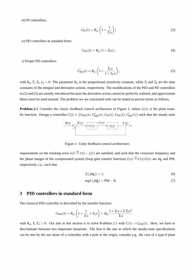
iii) PI controllers:
CPI(s) = Kp
(
1+1
Ti s
)
; (3)
iv) PD controllers in standard form:
CPD(s) = Kp (1+Td s) ; (4)
v) Proper PD controllers:
C′PD(s) = Kp
(
1+Td s
1+ τd s
)
; (5)
with Kp,Ti ,Td,τd > 0. The parameterKp is the proportional sensitivity constant, whileTi andTd are the time
constants of the integral and derivative actions, respectively. The modifications of the PID and PD controllers
in (2) and (5) are usually introduced because the derivative action cannot be perfectly realised, and approximate
filters must be used instead. The problem we are concerned with can be stated in precise terms as follows.
Problem 2.1 Consider the classic feedback control architecture in Figure 1, whereG(s) is the plant trans-
fer function. Design a controllerC(s) ∈ {CPID(s),C′PID(s),CPI(s),CPD(s),C′
PD(s)} such that the steady-state
R(s) Y(s)+−
U(s)E(s)C(s) G(s)
Figure 1: Unity feedback control architecture.
requirements on the tracking errore(t)def= r(t)− y(t) are satisfied, and such that the crossover frequency and
the phase margin of the compensated system (loop gain transfer function)L(s)def= C(s)G(s) areωg and PM,
respectively, i.e., such that
∣L( jωg)∣= 1, (6)
argL( jωg) = PM−π. (7)
3 PID controllers in standard form
The classical PID controller is described by the transfer function:
CPID(s) = Kp
(
1+1
Ti s+Td s
)
= Kp1+Ti s+Ti Td s2
Ti s
with Kp,Ti ,Td > 0. Our aim in this section is to solve Problem 2.1 withC(s) = CPID(s). Here, we have to
discriminate between two important situations. The first is the one in which the steady-state specifications
can be met by the use alone of a controller with a pole at the origin; consider e.g. the case of a type-0 plant
and the steady-state performance criterion of zero position error. In thiscase, the fact itself of using a PID
controller guarantees that the steady-state requirement is satisfied. The second case of interest is the one in
which the imposition of the steady-state specifications gives rise to a constraint on the Bode gainKidef= Kp/Ti of
CPID(s). This situation occurs, for example, in the case of a type-0 plant when the steady-state specification not
only requires zero position error, but also that the velocity error be equal to (or smaller than) a given non-zero
constant. A similar situation arises with constraints on the acceleration error for type-1 plants.
3.1 Steady-State requirements do not constrain Ki
First, we consider the case where the steady-state specifications do not lead to a constraint on the integral
constant of the PID controller. In order to compute the parameters of the PID controller, we writeG( jω) and
CPID( jω) in polar form as
G( jω) = ∣G( jω)∣e j argG( jω), CPID( jω) = M(ω)e j ϕ(ω).
The loop gain frequency response can be written asL( jω) = ∣G( jω)∣M(ω)e j (argG( jω)+ϕ(ω)). If the gain
crossover frequencyωg and the phase margin PM of the loop gain transfer functionL(s) are assigned, by (6-7)
it is found that∣L( jωg)∣ = 1 and PM= π +argL( jωg) must be satisfied. These two equations can be written
as
(i) Mg = 1/ ∣G( jωg)∣ ,
(ii) ϕg = PM−π −argG( jωg),
whereMgdef= M(ωg) andϕg
def= ϕ(ωg). In order to find the parameters of the controller such that(i)-(ii) are met,
equation
Mge j ϕg = Kp1+ j ωgTi −ω2
g Ti Td
j ωgTi(8)
must be solved inKp,Ti ,Td > 0. It is easy to see that in the solution to this problem there is a degree of freedom,
since by equating the real and imaginary parts of both sides of (8) we obtainthe pair of equations
ωgMgTi cosϕg = ωgKpTi , (9)
−Mg ωgTi sinϕg = Kp−Kp ω2g Ti Td (10)
in the three unknownsKp,Ti andTd. A possibility to carry out the design at this point is to freely assign one
of the unknowns and to solve (9-10) for the other two. However, from (9) it is easily seen thatKp cannot be
chosen arbitrarily. If we chooseTi , (9) givesKp = Mg cosϕg, and (10) leads to
Td =1+ωgTi tanϕg
Ti ω2g
.
However, in order to guaranteeKp > 0 andTd > 0, the angleϕg must be such that cosϕg > 0 andTi must be
chosen to be smaller than−1/(ωg tanϕg). These two conditions can be simultaneously satisfied only when
ϕg ∈ (−π/2,0). If we chooseTd, we getKp = Mg cosϕg and
Ti =1
ω2g Td −ωg tanϕg
,
which implies that in order to ensureTi > 0 we must chooseTd to be greater than tanϕg/ωg. Therefore,Td is
arbitrary whenϕg ∈ (−π/2,0), while whenϕg ∈ (0,π/2), we must chooseTd > tanϕg/ωg.
Another possibility to carry out the design of the PID controller in the case ofunconstrained integral
constant is to exploit the remaining degree of freedom so as to satisfy some further time or frequency domain
requirements. There are several ways to exploit this degree of freedom in the calculation of the parameters of
the controller. In the sequel, we consider two important situations: the first isthe one where the ratioTd/Ti is
chosen, so as to ensure, for example, that the zeros of the PID controller are real; the second is the one where
a gain margin constraint is to be satisfied.
3.1.1 Imposition of the ratio Td/Ti
A very convenient way to exploit the degree of freedom in the solution of (8) consists in the imposition of the
ratioσ def= Td/Ti . This is convenient since it is an easily established fact that whenTi ≥ 4Td, i.e., whenσ−1 ≥ 4,
the zeros of the PID controller are real (and coincident whenσ−1 = 4), and they are complex conjugate when
σ−1 < 4. In the following theorem, necessary and sufficient conditions are given for the solvability of Problem
2.1 in the case of a standard PID controller when the ratioσ is given. Moreover, closed-form formulae are
provided for the parameters of the PID controller to meet the specifications on PM,ωg andσ exactly.
Theorem 3.1 Let σ = Td/Ti be assigned. Equation (8) admits solutions in Kp,Ti ,Td > 0 if and only if
ϕg ∈(
−π2,π2
)
. (11)
If (11) is satsfied, the solution of (8) withσ fixed is given by
Kp = Mg cosϕg (12)
Ti =tanϕg+
√
tan2 ϕg+4σ2ωg σ
(13)
Td = Ti σ (14)
Proof: (Only if). As already observed, equating real part to real part and imaginary part to imaginary part in
(8) results in (9) and (10). SinceKp must be positive, from (9) – which can be written asKp = Mg cosϕg – we
get thatϕg must satisfy−π/2< ϕg < π/2. If this inequality is satisfied, it is also easy to see that (10) always
admits a positive solution. In fact, (10) can be written as the quadratic equation
ω2g σ T2
i −ωgTi tanϕg−1= 0, (15)
in Ti , that always admits two real solutions, one positive and one negative.
(If). From (12), it follows that (9) is satisfied. Moreover, since as aforementioned (10) can be writtes as (15)
and√
tan2 ϕ +4σ > ∣ tanϕ ∣, the positive solution is given by (13).
3.1.2 Imposition of the Gain Margin
Another possibility in the solution of the control problem in the case of unconstrainedKi is to fix the gain
margin to a certain value GM. To this end, the conditions argL( jωp) =−π and GM= ∣L( jωp)∣−1 on the loop
gain frequency response must be satisfied by definition of gain margin andphase crossover frequencyωp. By
writing againCPID( jω) = M(ω)e j ϕ(ω), it is found that these conditions are equivalent to
Mp =1
GM ∣G( jωp)∣, (16)
ϕp = −π −argG( jωp), (17)
whereMpdef= M(ωp) andϕp
def= ϕ(ωp). Therefore, now the parametersKp,Ti ,Td > 0 of the PID controller must
be determined so that (8) and
Mpe j ϕp = Kp1+ j ωpTi −ω2
p Ti Td
j ωpTi(18)
are simultaneously satisfied. By equating the real and the imaginary part of (8) and (18) we obtain (9), (10)
and the additional two equations
ωpMpTi cosϕp = ωpKpTi , (19)
−Mp ωpTi sinϕp = Kp−Kp ω2p Ti Td. (20)
From (9) and (19), we obtain the equation
Mg cosϕg = Mp cosϕp (21)
in the unknownωp. For the control problem to be solvable, it is required that equation (21) admits at least one
strictly positive solution. At first glance, equation (21) seems transcendental in ωp. However, a more careful
analysis reveals that the solution of (21) can be found by solving a polynomial equation inωp, as the following
lemma shows.
Lemma 3.1 Let G(s) be a rational function in s∈ ℂ. Then, (21) can be reduced to a polynomial equation in
ωp. Let n1 and m1 represent the number of real poles/zeros of G(s), and let n2 and m2 represent the number
of complex conjugate pairs of poles/zeros of G(s), respectively, and letν ∈ ℤ be the number of poles at the
origin of G(s) (with the understanding that ifν < 0, the transfer function has−ν zeros at the origin). Then,
the degree of the polynomial equation (21) is at most{
max{ν + l , 2m1+4m2} if ν ≥ 0
max{l ,−ν +2m1+4m2} if ν < 0
where l= m1+m2+n1+n2.
Proof: Let us write the transfer function of the plant in the Bode real form:
G(s) =KB
sν
m1
∏i=1
(1+ τi s)m2
∏i=1
(
1+2ζi
ωn,is+
s2
ω2n,i
)
n1
∏i=1
(1+ τi s)n2
∏i=1
(
1+2ζi
ωn,is+
s2
ω2n,i
)
with ν ∈ ℤ. In the Bode real form given above, the parametersτi andτi are the time constants associated with
the real poles/zeros,ζi and ζi are the damping ratios andωn,i andωn,i are the natural frequencies associated
with the complex conjugate pairs of poles/zeros ofG(s). It follows that
Mp =ων
p
KB
n1
∏i=1
√
1+ω2p τ2
i
n2
∏i=1
√
√
√
⎷
(
1−ω2
p
ω2n,i
)2
+4ζ 2i
ω2p
ω2n,i
GMm1
∏i=1
√
1+ω2p τ2
i
m2
∏i=1
√
√
√
⎷
(
1−ω2
p
ω2n,i
)2
+4ζ 2i
ω2p
ω2n,i
and
ϕp = −hπ +ν
∑i=1
(
−π2
)
+m1
∑i=1
arctan(ωp τi)+m2
∑i=1
arctan2ζiωp ωn,i
ω2p− ω2
n,i
−n1
∑i=1
arctan(ωp τi)−n2
∑i=1
arctan2ζiωp ωn,i
ω2p−ω2
n,i
where the integerh depends on the sign ofKB and on the sign of the real parts of the second order terms of the
frequency responseG( j ω). As such,ϕp can be written as
ϕp =−(h+ν − ν)π +ν
∑i=1
(
−π2
)
+l
∑j=0
Φ j
for suitably defined anglesΦ j , wherel = m1+m2+n1+n2 andν is either equal to 0 whenν is even and equal
to 1 if ν is odd. Therefore,
cosϕp =
{
(−1)h+ν−1 cos(
∑lj=0 Φ j
)
if ν is even
(−1)h+ν sin(
∑lj=0 Φ j
)
if ν is odd(22)
In view of the well-known formulae
cos
(
l
∑j=0
Φ j
)
= ∑evenk∈{0,...,l}
(−1)k2 ∑
S⊆{1,... l}∣S∣=k
(
∏j∈S
sinΦ j ∏j /∈S
cosΦ j
)
(23)
sin
(
l
∑j=0
Φ j
)
= ∑oddk∈{0,...,l}
(−1)k2 ∑
S⊆{1,... l}∣S∣=k
(
∏j∈S
sinΦ j ∏j /∈S
cosΦ j
)
, (24)
we obtain
cosϕp =p
∑j=1
(
m1
∏i=1
f ai, j(arctan(ωp τi))
m2
∏i=1
f bi, j(arctan
2ζiωp ωn,i
ω2p− ω2
n,i
)
⋅n1
∏i=1
f ci, j(arctan(ωp τi))
n2
∏i=1
f di, j(arctan
2ζiωp ωn,i
ω2p−ω2
n,i
)
)
where f ki, j (with k ∈ {a,b,c,d}) are either sine or cosine functions andp= 2m1+m2+n1+n2−1. From the gonio-
metric identities
sinarctanθ =θ√
1+θ 2cosarctanθ =
1√1+θ 2
it follows that cosϕp can be written as
cosϕp =F(ωp)
n1
∏i=1
√
1+ω2p τ2
i
n2
∏i=1
√
√
√
⎷
(
1−ω2
p
ω2n,i
)2
+4ζ 2i
ω2p
ω2n,i
m1
∏i=1
√
1+ω2p τ2
i
m2
∏i=1
√
√
√
⎷
(
1−ω2
p
ω2n,i
)2
+4ζ 2i
ω2p
ω2n,i
whereF(ωp) is a polynomial function ofωp given by sums of products of the typeωp τi , ωp τi , ζi ωp/ωn,i and
ζi ωp/ωn,i . Its degree depends on the term containing the largest number of sine factors in the sum (22). From
(23-24) it is easy to establish that whenν is even,
degF =
{
l if l is even
l −1 if l is odd
and, whenν is odd,
degF =
{
l −1 if l is even
l if l is odd
Therefore, the degree ofF(ωp) is at mostl . Hence,
Mpcosϕp =ων
p F(ωp)
KBGMm1
∏i=1
(1+ω2pτ2
i )m2
∏i=1
⎡
⎣
(
1−ω2
p
ω2n,i
)2
+4ζ 2i
ω2p
ω2n,i
⎤
⎦
Therefore, (21) is a polynomial equation inωp. In view of possible cancellations, the degree of this equation
is not greater than max{ν + l , 2m1+4m2} if ν ≥ 0 and max{l ,−ν +2m1+4m2} if ν < 0.
Remark 3.1 If the transfer function of the process is given by the product of a rational functionG(s), and
a delaye−t0 s, i.e., if G(s) = G(s)e−t0 s, equation (21) is not polynomial inωp, and it needs to be solved
numerically. More details about this case are given in Section 9.
Theorem 3.2 Consider Problem 2.1 with the additional specification on the gain margin GM. Equations (8)
and (18) admit solutions in Kp,Ti ,Td > 0 if and only ifϕg ∈ (−π/2,π/2) and (21) admits a positive solution
ωp such that⎧
⎨
⎩
ωp < ωg
ωg tanϕg > ωp tanϕp
ωp tanϕg > ωg tanϕp
or
⎧
⎨
⎩
ωp > ωg
ωg tanϕg < ωp tanϕp
ωp tanϕg < ωg tanϕp
(25)
If ϕg ∈ (−π/2,π/2) and (25) is satisfied, the control problem admits solutions with a PID controller, whose
parameters can be computed as
Kp = Mg cosϕg (26)
Ti =ω2
g −ω2p
ωg ωp (ωp tanϕg−ωg tanϕp)(27)
Td =ωg tanϕg−ωp tanϕp
ω2g −ω2
p(28)
Proof: (Only if). As already seen, a necessary condition for the problem to admit solutions isthat ωp is a
solution of (21). From (9) and (10), and from (19) and (20), we obtain
−ωgTi tanϕg = 1−ω2g Ti Td, (29)
−ωpTi tanϕp = 1−ω2p Ti Td. (30)
By solving (29) and (30) inTi andTd, we obtain (26-28). ForKp to be positive, it is necessary thatϕg ∈(−π/2,π/2). Moreover, the time constantsTi andTd are positive ifωg andωp satisfy (25).
(If). It is a matter of straighforward substitution of (26-28) into (9), (10), (19) and (20).
Remark 3.2 In view of the constraintKp > 0, (25) can be written as follows:
If ωg > ωp: one of the following conditions must hold:
∙ ϕg,ϕp ∈(
0, π2
)
andϕg > ϕp;
∙ ϕg ∈(
0, π2
)
andϕp ∈(
−π2 ,0)
;
∙ ϕg,ϕp ∈(
−π2 ,0)
andϕg < ϕp.
If ωg < ωp: one of the following conditions must hold:
∙ ϕg,ϕp ∈(
0, π2
)
andϕg < ϕp;
∙ ϕg ∈(
−π2 ,0)
andϕp ∈(
0, π2
)
;
∙ ϕg,ϕp ∈(
−π2 ,0)
andϕg > ϕp.
3.2 Steady-State requirements constrain Ki
Now, the Bode gainKi = Kp/Ti is determined via the imposition of the steady-state requirements; for example,
for type-0 (resp. type-1) plants,Ki is computed via the imposition of the velocity error (resp. acceleration
error).
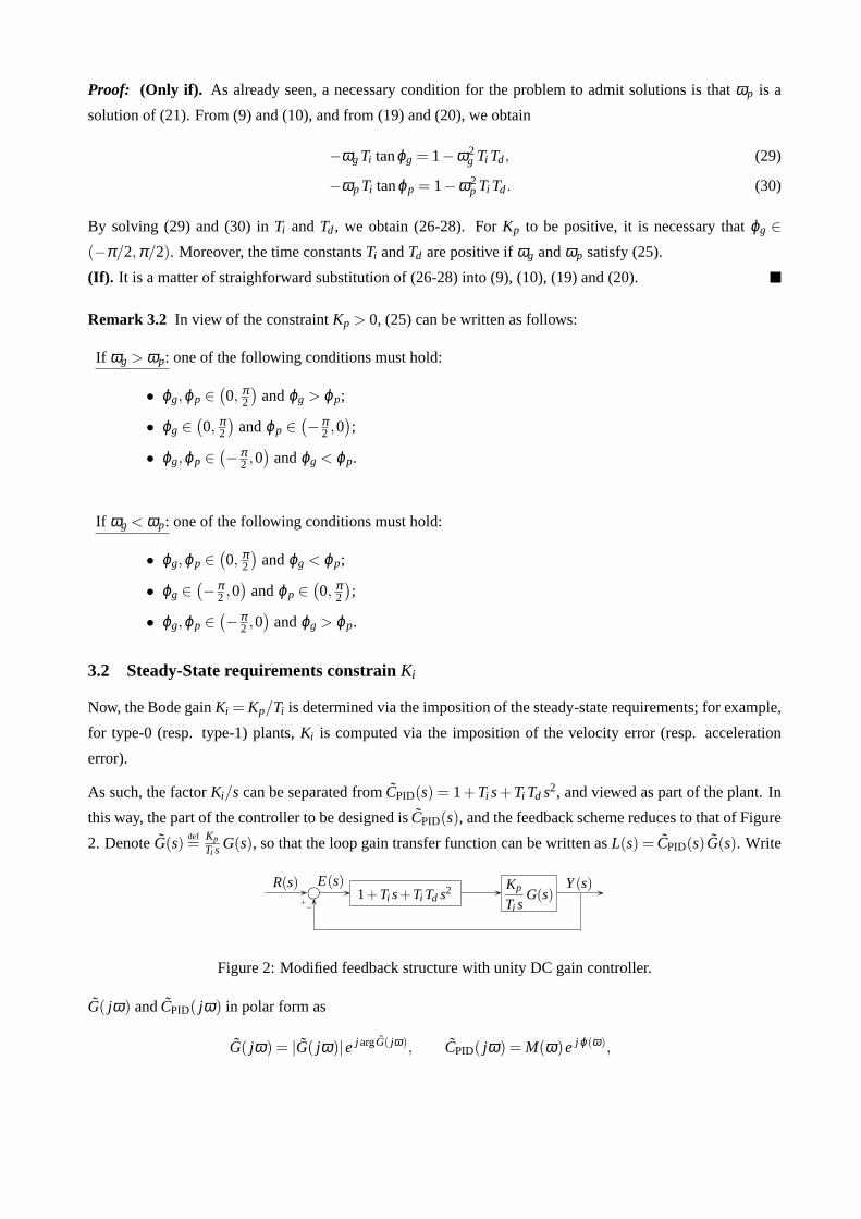
As such, the factorKi/s can be separated fromCPID(s) = 1+Ti s+Ti Td s2, and viewed as part of the plant. In
this way, the part of the controller to be designed isCPID(s), and the feedback scheme reduces to that of Figure
2. DenoteG(s)def=
Kp
Ti sG(s), so that the loop gain transfer function can be written asL(s) = CPID(s)G(s). Write
R(s) Y(s)+−
E(s)1+Ti s+Ti Td s2 Kp
Ti sG(s)
Figure 2: Modified feedback structure with unity DC gain controller.
G( jω) andCPID( jω) in polar form as
G( jω) = ∣G( jω)∣e j argG( jω), CPID( jω) = M(ω)e j ϕ(ω),
so that the loop gain frequency response can be written asL( jω) = ∣G( jω)∣M(ω)e j (argG( jω)+ϕ(ω)). If the
crossover frequencyωg and the phase margin PM of the loop gain transfer functionL(s) are assigned, the
equations∣L( jωg)∣= 1 and PM= π +argL( jωg) must be satisfied. These can be written as
(i) Mg = 1/ ∣G( jωg)∣ ,
(ii) ϕg = PM−π −argG( jωg),
whereMgdef= M(ωg) andϕg
def= ϕ(ωg). Alternatively,Mg andϕg can be computed as functions of the frequency
response ofG(s) at ω = ωg:
Mg =
∣
∣
∣
∣
Kp
Ti j ωgG( jωg)
∣
∣
∣
∣
−1
=ωg
Ki ∣G( jωg)∣(31)
ϕg = PM−π −arg
[
Kp
Ti j ωgG( jωg)
]
= PM− π2−argG( jωg), (32)
sinceKp,Ti > 0. In order to find the parameters of the controller such that(i)-(ii) are met, equation
Mgej ϕg = 1+ j ωgTi −Ti Td ω2g (33)
must be solved inTi > 0 andTd > 0. The closed-form solution to this problem is given in the following
theorem.
Theorem 3.3 Equation (33) admits solutions in Ti > 0 and Td > 0 if and only if
0< ϕg < π and Mg cosϕg < 1. (34)
If (34) are satisfied, the solution of (33) is given by
Kp = Ki1
ωgMgsinϕg (35)
Ti =1
ωgMgsinϕg (36)
Td =1−Mg cosϕg
ωgMg sinϕg. (37)
The two conditions (34) can be alternatively written as
ϕg ∈(
arccos1
Mg, π)
if Mg > 1,
ϕg ∈ (0, π) if Mg < 1,
In fact, whenϕg ∈ (0,π/2), condition cosϕg < 1/Mg is always satisfied whenMg < 1, and is satisfied when
ϕg > arccos(1/Mg) whenMg > 1. Whenϕg ∈ (π/2,π), the condition cosϕg < 1/Mg is always satisfied since
cosϕg < 0 and(1/Mg)> 0. As a consequence, we have the following.
Corollary 3.1 When the ratio Kp/Ti is assigned, Problem 2.1 admits solutions if and only if
∙ argG( jωg) ∈(
PM− 32
π, PM− π2
)
if ∣G( jωg)∣>ωg
Ki;
∙ argG( jωg) ∈(
PM− 32
π, PM− π2−arccos
Ki ∣G( jωg)∣ωg
)
if ∣G( jωg)∣<ωg
Ki.
When the steady-state specifications lead to a constraint on the ratioKi = Kp/Ti , there are no degrees of
freedom that can be exploited to assignσ = Td/Ti . As a result, in this case the design technique based on the
imposition of the phase margin and crossover frequency can lead to PID controllers with either real or complex
conjugate zeros. However, in standard practice it is desirable to work withPID controllers with real zeros. The
following theorem establishes necessary and sufficient conditions on theproblem data and specifications for
the zeros of the PID controller to be real.
Theorem 3.4 The zeros of the PID controller are real if and only if
∙ ∣G( jωg)∣<ωg
Ki;
∙ argG( jωg) ∈(
PM− π2−arccos
2Ki ∣G( jωg)∣−ωg
ωg,PM− π
2
)
.
Proof: The discriminantTi (Ti − 4Td) of the numerator ofCPID(s) is greater or equal to zero if and only if
Ti ≥ 4Td. Using (36-37), this inequality becomes
1ωg
Mg sinϕg ≥ 41
ωg
1−Mg cosϕg
Mg sinϕg,
which leads to
M2g cos2 ϕg−4Mg cosϕg+(4−M2
g)≤ 0. (38)
Solving (38) in cosϕg yields
2−Mg
Mg≤ cosϕg ≤
2+Mg
Mg.
However,2+Mg
Mg> 1. Moreover,2−Mg
Mg>−1 and2−Mg
Mg< 1 if and only ifMg > 1. Hence,
[
2−Mg
Mg,2+Mg
Mg
]
∩ [−1,1] ∕= /0
only whenMg > 1. Hence, whenMg < 1 the inequality (38) is never satisfied, while whenMg > 1, (38) holds
if and only if cosϕg >2−Mg
Mg. It follows that the zeros of the PID controller are real if and only if
Mg > 1 and 0< ϕg < arccos2−Mg
Mg. (39)
The result is then a matter of substitution of the definitions ofMg andϕg in (39).
4 Proper PID controllers
The transfer function of the PID controller in standard form is not proper. To obtain a proper approximation of
CPID(s), usually a further real pole is introduced in the derivative term:
C′PID(s) = Kp
(
1+1
Ti s+
Td s1+ τd s
)
=Kp
Ti sTi (Td + τd)s2+(Ti + τd)s+1
1+ τd s(40)
with Kp,Ti ,Td,τd > 0. Due to the additional poles=−1/τd, the transfer functionC′PID(s) is now (bi-)proper.
Typically, to obtain a good approximation of the derivative action, the frequency associated with the further
pole is chosen to be much higher than the frequencies of all other poles andzeros of the loop gain transfer
function. As such, the parameterτd is usually very small. Our aim here is to solve Problem 2.1 using a con-
troller C(s) =C′PID(s). For the sake of brevity, we only consider the case where the steady-state specifications
lead to an assignment of the Bode gainKp/Ti . By defining
C′PID(s) =
Ti (Td + τd)s2+(Ti + τd)s+11+ τd s
andL(s) = C′PID(s)G(s), and by expressingG( jω) andC′
PID( jω) in polar form,Mg andϕg can be defined as
in (31) and (32). Then, in order to find the parameters of the controller, equation
Mgej ϕg =−Ti (Td + τd)ω2
g + j (Ti + τd)ωg+1
1+ j ωg τd(41)
must be solved inTi > 0 andTd > 0. The closed-form solution to this problem is given in the following
theorem.
Theorem 4.1 Equation (41) admits solutions in Ti > 0 and Td > 0 if and only if
τd <Mg sinϕg
ωg(1−cosϕg). (42)
If (42) is satisfied, the solution of (41) is given by
Kp =Ki Mg sinϕg
ωg− τd (1−Mg cosϕg) (43)
Ti =Mg sinϕg
ωg−Ki τd (1−Mg cosϕg) (44)
Td =1+ω2
g τ2d
ωg
(
Mg sinϕg
1−Mg cosϕg−ωg τd
) (45)
Proof: It is easy to see that
CPID( jω) =[
−Ti (Td + τd)ω2g + j (Ti + τd)ωg+1
]
(1− j ωg τd)
(1+ j ωg τd)(1− j ωg τd)=
−Ti Td ω2+ j ω ,Ti +1+ jω3 τd Ti Td + j ω3Ti τ2d +ω2 τ2
d
1+ω2τ2d
.
Hence, by (41) we get
Mg cosϕg(1+ω2gτ2
d) = −Ti Td ω2g +1+ω2
gτ2d ,
Mg sinϕg(1+ω2gτ2
d) = ωgTi +ω3g τd Ti Td +ω3
g Ti τ2d .
Solving both equations inTi and equating the results yield
(1−Mg cosϕg)(1+ω2gτ2
d)
Td ω2g
=Mg sinϕg(1+ω2
gτ2d)
ωg(1+ω2gτd Td +ω2
gτ2d),
that can be solved to getTd. This gives (45).
Finally, the proportional sensitivityKp can be computed from the ratioKp/Ti using the value ofTi thus
found.
Example 4.1 Consider the plant described by the transfer function
G(s) =1
s(s+2),
and consider the problem of determining the parameters of a PID controller that exactly achieves a phase
margin of 45∘ and gain crossover frequencyωg = 30rad/s in the two situations:
∙ the acceleration error is equal to 0.005.
∙ the velocity error is equal to zero; first use the remaining degree of freedom to assign the ratioTi/Td = 16,
and then to impose a gain margin equal to 3.
Consider the first problem. The expression of the acceleration error is
ea∞ =
1lims→0s2L(s)
=1
lims→0s2Kp1+Ti s+Ti Td s2
Ti s2(s+2)
=2Ti
Kp.
Then,ea∞ = 0.005 impliesKi = Kp/Ti = 400. DefineG(s) = Ki G(s)/s. ComputeMg = 30/Ki ∣G(30 j)∣ =
9√
904/4 andϕg = PM−π/2−argG(30 j) = π/4+arctan15. Using Theorem 3.3, it is seen that the time
constants of the PID controller are
Ti =Mg sinϕg
30=
12
5√
2, Td =
1−Mgcosϕg
30Mg sinϕg=
√2+632160
.
The zeros of the PID controller are real sinceTi is greater than 4Td. From the ratioKp/Ti = 400, we find
Kp = 400Ti = 960/√
2. The transfer function of the PID controller is
CPID(s) =960√
2
(
1+5√
212s
+
√2+632160
s)
.
Let us now solve the same problem with a PID controller with an additional pole as in (40). We first need
to chooseτd to be smaller than the quantity
Mg sinϕg
ωg(1−Mg cosϕg)≃ 0.0373.
10−1
100
101
102
−100
−50
0
50
100
10−1
100
101
102
−180
−160
−100
−135
−80
PM
ωg
∣ ⋅ ∣dB
∠
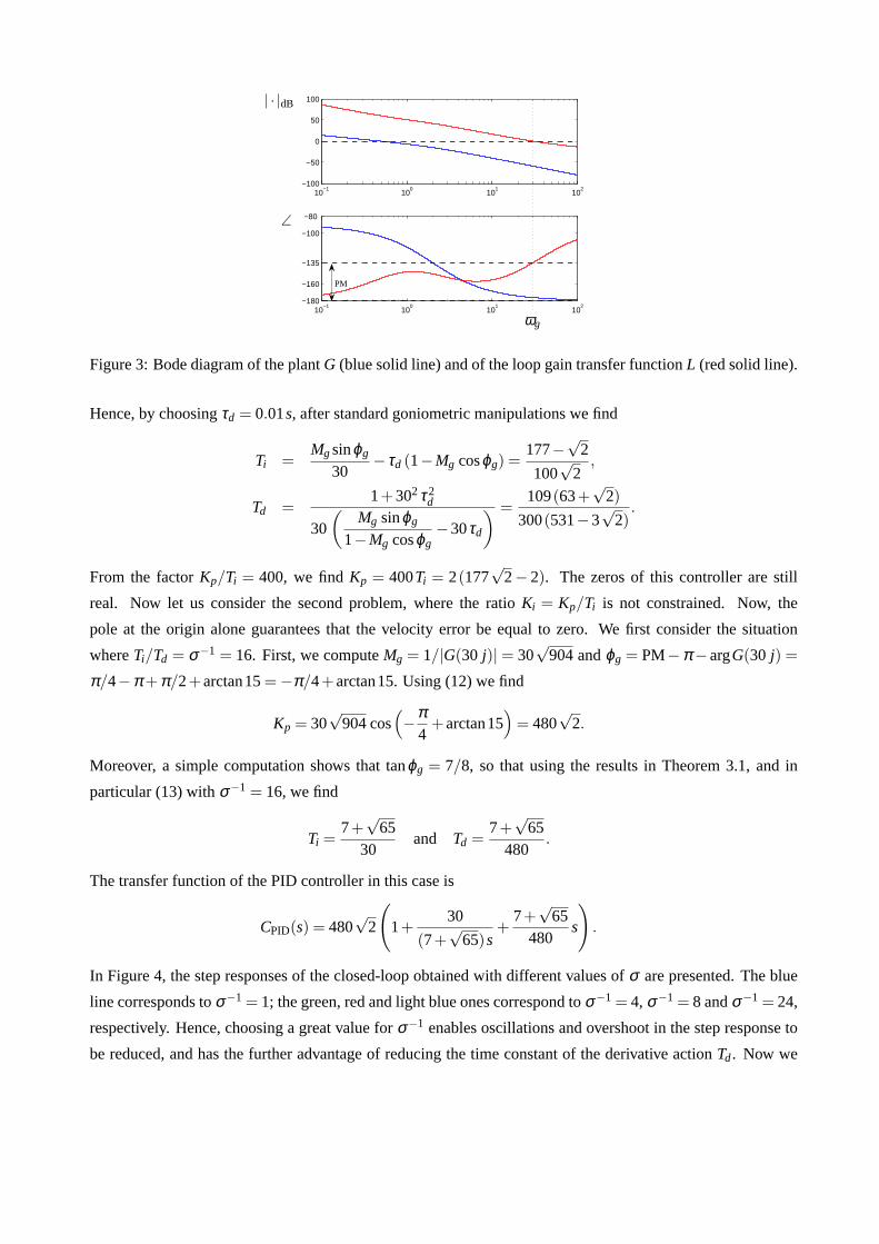
Figure 3: Bode diagram of the plantG (blue solid line) and of the loop gain transfer functionL (red solid line).
Hence, by choosingτd = 0.01s, after standard goniometric manipulations we find
Ti =Mgsinϕg
30− τd (1−Mg cosϕg) =
177−√
2
100√
2,
Td =1+302 τ2
d
30
(
Mg sinϕg
1−Mg cosϕg−30τd
) =109(63+
√2)
300(531−3√
2).
From the factorKp/Ti = 400, we findKp = 400Ti = 2(177√
2− 2). The zeros of this controller are still
real. Now let us consider the second problem, where the ratioKi = Kp/Ti is not constrained. Now, the
pole at the origin alone guarantees that the velocity error be equal to zero. We first consider the situation
whereTi/Td = σ−1 = 16. First, we computeMg = 1/∣G(30 j)∣ = 30√
904 andϕg = PM−π −argG(30 j) =
π/4−π +π/2+arctan15=−π/4+arctan15. Using (12) we find
Kp = 30√
904 cos(
−π4+arctan15
)
= 480√
2.
Moreover, a simple computation shows that tanϕg = 7/8, so that using the results in Theorem 3.1, and in
particular (13) withσ−1 = 16, we find
Ti =7+
√65
30and Td =
7+√
65480
.
The transfer function of the PID controller in this case is
CPID(s) = 480√
2
(
1+30
(7+√
65)s+
7+√
65480
s
)
.
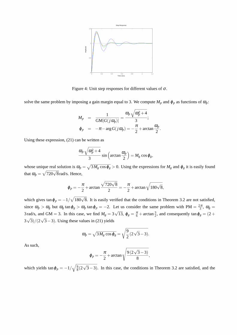
In Figure 4, the step responses of the closed-loop obtained with different values ofσ are presented. The blue
line corresponds toσ−1 = 1; the green, red and light blue ones correspond toσ−1 = 4, σ−1 = 8 andσ−1 = 24,
respectively. Hence, choosing a great value forσ−1 enables oscillations and overshoot in the step response to
be reduced, and has the further advantage of reducing the time constantof the derivative actionTd. Now we
0 0.2 0.4 0.6 0.8 1 1.20
0.5
1
1.5
Step Response
Time (sec)
Am
plitu
de
Figure 4: Unit step responses for different values ofσ .
solve the same problem by imposing a gain margin equal to 3. We computeMp andϕp as functions ofωp:
Mp =1
GM∣G( j ωp)∣=
ωp
√
ω2p+4
3;
ϕp = −π −argG( j ωp) =−π2+arctan
ωp
2.
Using these expression, (21) can be written as
ωp
√
ω2p+4
3sin(
arctanωp
2
)
= Mg cosϕg,
whose unique real solution isωp =√
3Mg cosϕg > 0. Using the expressions forMg andϕg it is easily found
thatωp =√
720√
8rad/s. Hence,
ϕp =−π2+arctan
√
720√
82
=−π2+arctan
√
180√
8,
which gives tanϕp = −1/√
180√
8. It is easily verified that the conditions in Theorem 3.2 are not satisfied,
sinceωp > ωg but ωg tanϕg > ωp tanϕp = −2. Let us consider the same problem with PM= 2π3 , ωg =
3rad/s, and GM= 3. In this case, we findMg = 3√
13, ϕg =π6 +arctan3
2, and consequently tanϕg = (2+
3√
3)/(2√
3−3). Using these values in (21) yields
ωp =√
3Mg cosϕg =
√
92(2√
3−3).
As such,
ϕp =−π2+arctan
√
9(2√
3−3)8
,
which yields tanϕp = −1/√
98(2
√3−3). In this case, the conditions in Theorem 3.2 are satisfied, and the
parameters of the PID controller can be computed in closed form as
Kp = Mg cosϕg =32(2√
3−3)
Ti =ω2
g −ω2p
ωg ωp (ωp tanϕg−ωg tanϕp)=
5−2√
3
10+9√
3
Td =ωg tanϕg−ωp tanϕp
ω2g −ω2
p=
26√
3
144√
3−243.
SinceTi < 4Td, the zeros of the PID controller are complex conjugate.
Example 4.2 Consider the example in [16], where a PID controller must be used for the plant
G(s) =3
s(s2+4s+5)
to achieve the following control objectives:i) acceleration constantKa = 2; ii) gain crossover frequencyωg =
2.5rad/s and phase margin PM= 48∘. First, the steady-state specification fixes the ratioKi = Kp/Ti , as
Ka = lims→0
(
s2CPID(s)G(s))
=35
Kp
Ti= 2,
which in turn impliesKi = Kp/Ti = 10/3. FromG(52 j) = 24/(−25 j −200), we get
Mg =52
Ki ∣G(52 j)∣
=25
√65
32
ϕg = PM− π2−argG(
52
j) =−3730
π +arctan18.
From sin(3730 π) =−sin( 7
30 π) =−k1/8 and cos(3730 π) =−cos( 7
30 π) =−k2/4, with
k1 = 1−√
5+
√
30+6√
5,
k2 =
√
7−√
5+√
6(5−√
5),
we obtain
sinϕg =1√65
(
k1−k2
4
)
,
cosϕg = − 1√65
(
2k2+k1
8
)
.
Plugging these values into (36-37), we obtain closed-form expressionsfor all the parameters of the PID con-
troller
Kp =2524
(
k1−k2
4
)
,
Ti =516
(
k1−k2
4
)
,
Td =256+25k1+400k2
500k1−125k2.
Notice that, differently from [16], the solution provided here is given in finite terms. This ensures that the
desired crossover frequency and the desired phase margin are achieved exactly.
Let us now consider the same plant, for which a PID controller must be designed to achieve a gain crossover
frequency crossover frequencyωg = 1rad/s, a phase margin PM= 30∘, and a gain margin GM= 3. It is easily
seen thatMg = 4√
2/3 andϕg =−π/12, so that tan(ϕg) =−(√
2−√
6)/4. It is easily seen that (21) admits a
positive solution
ωp =
√
3GM4
Mg cosϕg =
√
3
√3+12
.
Therefore,
ϕp =−π2+arctan
4ωp
5−ω2p.
Sinceωp <√
5, we find that
tanϕp =3√
3−7
4√
6(√
3+1).
A simple computation yields
Kp =2√
3+23
,
Ti =4(1+3
√3)
15√
3−19,
Td =9−5
√3
4(1+3√
3).
In this case,Ti > 4Td; the zeros of the PID controller are real and strictly negative.
5 PI controllers
The synthesis techniques presented in the previous sections can be adapted to the design of PI controllers for
the imposition of phase margin and crossover frequency of the loop gain transfer function. This can be done,
however, only when the steady-state specifications do not lead to the imposition of the Bode gain of the loop
gain transfer function. The transfer function of a PI controller is
CPI(s) = Kp
(
1+1
Ti s
)
= KpTi s+1
Ti s.
By definingG(s) = G(s)/s, it is found
Mg =1
∣G( jωg)∣=
ωg
∣G( jωg)∣,
ϕg = PM−π −argG( jωg) = PM− π2−argG( jωg).
To find the parameters of the PI controller, equation
Mge j ϕg = Kpj Ti ωg+1
Ti(46)
must be solved inKp > 0 andTi > 0.
−60
−40
−20
0
20
40
60
(dB
)
10−2
10−1
100
101
102
103
104
−270
−225
−180
−135
−90 (
deg)
(rad/sec)
GM
PM
ωg ωp
∣ ⋅ ∣dB
∠
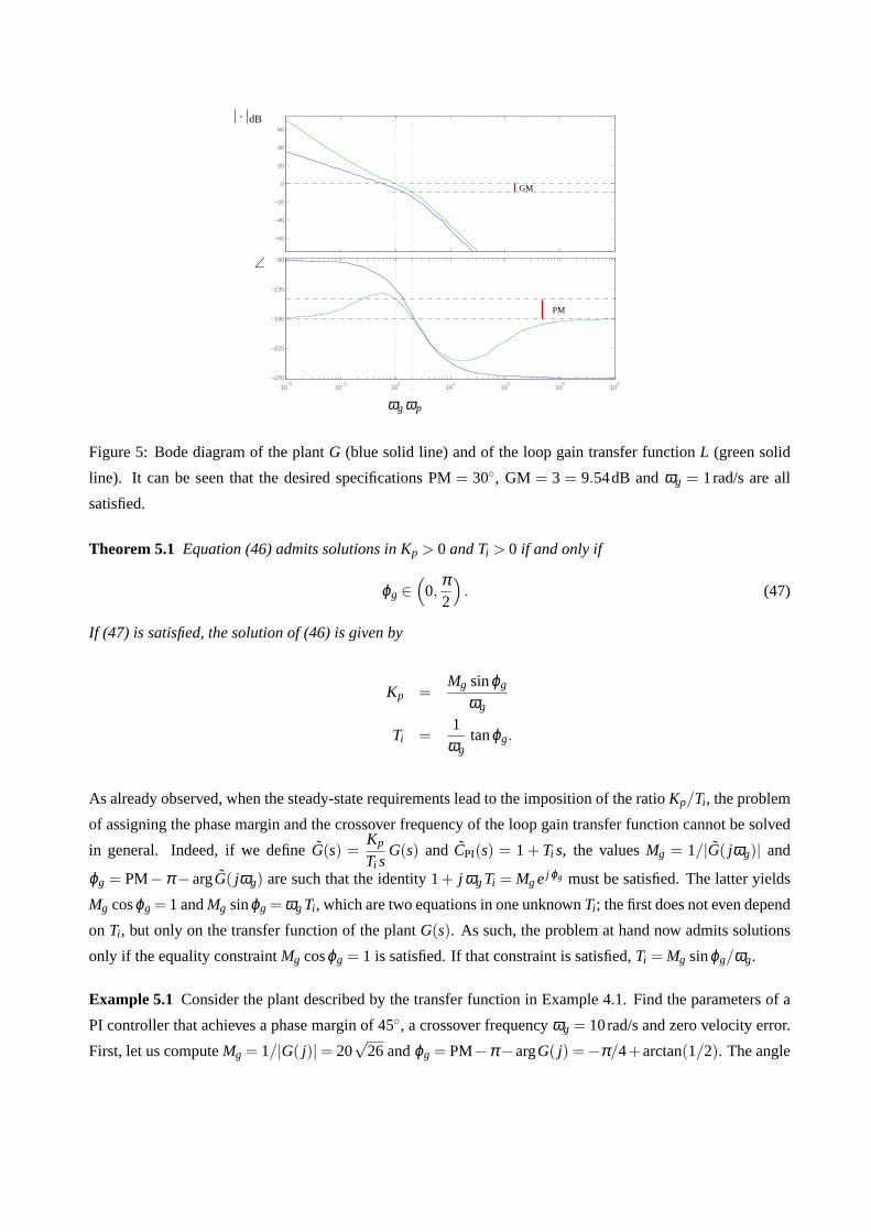
Figure 5: Bode diagram of the plantG (blue solid line) and of the loop gain transfer functionL (green solid
line). It can be seen that the desired specifications PM= 30∘, GM = 3 = 9.54dB andωg = 1rad/s are all
satisfied.
Theorem 5.1 Equation (46) admits solutions in Kp > 0 and Ti > 0 if and only if
ϕg ∈(
0,π2
)
. (47)
If (47) is satisfied, the solution of (46) is given by
Kp =Mg sinϕg
ωg
Ti =1
ωgtanϕg.
As already observed, when the steady-state requirements lead to the imposition of the ratioKp/Ti , the problem
of assigning the phase margin and the crossover frequency of the loop gain transfer function cannot be solved
in general. Indeed, if we defineG(s) =Kp
Ti sG(s) and CPI(s) = 1+ Ti s, the valuesMg = 1/∣G( jωg)∣ and
ϕg = PM−π −argG( jωg) are such that the identity 1+ j ωgTi = Mgej ϕg must be satisfied. The latter yields
Mg cosϕg = 1 andMg sinϕg =ωgTi , which are two equations in one unknownTi ; the first does not even depend
on Ti , but only on the transfer function of the plantG(s). As such, the problem at hand now admits solutions
only if the equality constraintMg cosϕg = 1 is satisfied. If that constraint is satisfied,Ti = Mg sinϕg/ωg.
Example 5.1 Consider the plant described by the transfer function in Example 4.1. Find the parameters of a
PI controller that achieves a phase margin of 45∘, a crossover frequencyωg = 10rad/s and zero velocity error.
First, let us computeMg = 1/∣G( j)∣= 20√
26 andϕg = PM−π −argG( j) =−π/4+arctan(1/2). The angle
ϕg lies in (0,π/2), so that a PI controller meeting the specifications exists. The parameters canbe found with
Kp =Mg sinϕg
ωg= 40
√2,
Ti =1
ωgtanϕg =
115
.
The transfer function of the PI controller is
CPI(s) =Mg ωg cosϕg+Mg sinϕgs
ωgs= 40
√2
s+15s
.
Notice that, since in this case we haveMg cosϕg =√
3 cos(−π/4+ arctan1/2) ∕= 1, we cannot solve the
problem with constraints onKi .
6 PD controllers
As for the design of PI controllers, the synthesis techniques presented for the imposition of phase margin and
crossover frequency of the loop gain transfer function can be used for PD controllers only when the steady-
state specifications do not lead to the imposition of the proportional sensitivityKp. The transfer function of a
PD controller is
CPD(s) = Kp (1+Td s) .
To find the parameters of the PD controller, the equation
Mge j ϕg = Kp (1+ j Td ωg) (48)
must be solved inKp > 0 andTd > 0.
Theorem 6.1 Equation (48) admits solutions in Kp > 0 and Td > 0 if and only if
ϕg ∈(
0,π2
)
. (49)
If (49) is satisfied, the solution of (48) is given by
Kp = Mg cosϕg
Td =1
ωgtanϕg.
When the imposition of the steady-state specifications lead to a sharp constraint on Kp, and defineG(s) =
KpG(s) andCPD(s) = 1+Td s, the valuesMg = 1/∣G( jωg)∣ andϕg = PM−π −argG( jωg) lead to the identity
1+ j ωgTd = Mgej ϕg, which in turn leads to the two equationsMg cosϕg = 1 andMg sinϕg = ωgTd, so that
the problem admits solutions only if the constraintMg cosϕg = 1 is satisfied. In that case,Td = Mg sinϕg/ωg.

7 Proper PD controllers
Now we consider an alternative form of the PD controller, described by the transfer function:
C′PD(s) = Kp
(
1+Td s
1+ τd s
)
= Kp1+(Td + τd)s
1+ τd s, (50)
with Kp,Td,τd > 0. In this case, the proposed method can be applied even in the presence of steady-state
requirements on the position error for type-0 plants, on the velocity error for type-1 plants, and on the accel-
eration error for type-2 plants. In fact, the transfer functionC′PD(s) is exactly that of a lead network. Since
the transfer functionC′PD(s) does not contain poles at the origin, usually the steady-state specificationslead to
constraints on the proportional sensitivityKp. In that case, let us defineG(s) = KpG(s), and
C′PD(s) =
1+(Td + τd)s1+ τd s
.
If we also setC′PD( jω) = M(ω)ej ϕ(ω), by imposing∣L( jωg)∣ = 1 and PM= π +argL( jωg), we find that, as
before, in order to find the parameters of the controller, equation
Mgej ϕg =1+ j (Td + τd)ωg
1+ j τd ωg(51)
must be solved inTd,τd > 0.
Theorem 7.1 Equation (51) admits solutions Td,τd > 0 if and only if
Mg > 1, ϕg ∈(
0,π2
)
, Mg >1
cosϕg. (52)
If (52) are satisfied, the solution of (51) is given by
Td =M2
g −2Mg cosϕg+1
Mg ωg sinϕg
τd =Mg cosϕg−1Mg ωg sinϕg
8 Graphical and approximate solution to the design problem
The synthesis methods developed in the previous sections are based on closed-form formulae for the compu-
tation of the parameters of the PID controller. In this regard, it could be argued that often a full knowledge
of the dynamics of the plant is not available in practice and therefore the presented closed-form formulae are
of little interest. On the contrary, the approach presented here still offersa solution even when the model of
the plant is not exactly known, which is may be based on (i) graphical considerations similar in spirit to those
considered in the literature [16] (but that can be carried out onanyof the standard diagrams for the frequency
response), (ii) on the approximation of the plant with a first or second order transfer function [7], or even (iii)
on the results of an experiment conducted on the plant in the same spirit of theZiegler and Nichols methods,
[18]. In this and in the following section we discuss these issues.
As already mentioned, a graphical version of the method presented in this paper can implemented using
any of the frequency domain plots usually employed in control to representthe frequency response dynamics,
i.e., Bode diagrams, Nyquist diagrams or Nichols charts. This is due to the fact that the formulae used to derive
the parameters of the PID controller are expressed in terms of the magnitude and the argument of the frequency
response of the plant at a given crossover frequency, which is readable over any of these diagrams.
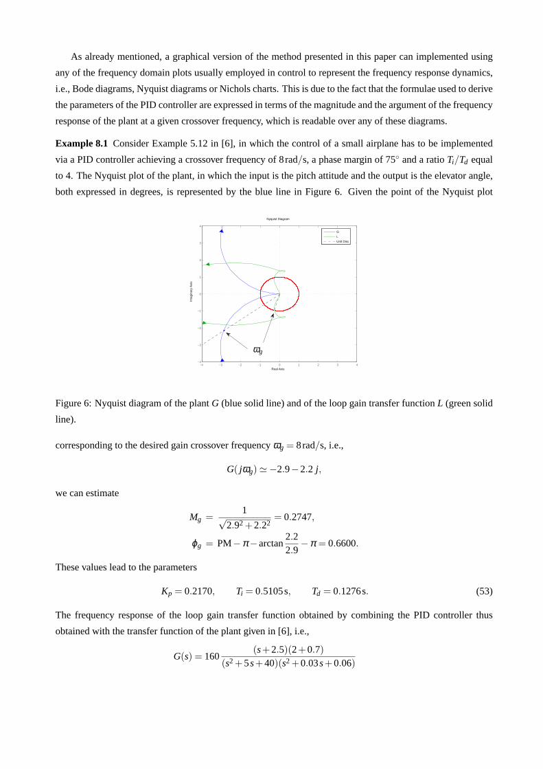
Example 8.1 Consider Example 5.12 in [6], in which the control of a small airplane has to beimplemented
via a PID controller achieving a crossover frequency of 8rad/s, a phase margin of 75∘ and a ratioTi/Td equal
to 4. The Nyquist plot of the plant, in which the input is the pitch attitude and the output is the elevator angle,
both expressed in degrees, is represented by the blue line in Figure 6. Given the point of the Nyquist plot
Nyquist Diagram
Real Axis
Imag
inar
y A
xis
−4 −3 −2 −1 0 1 2 3 4−4
−3
−2
−1
0
1
2
3
4
G
L
Unit Disc
ωg
Figure 6: Nyquist diagram of the plantG (blue solid line) and of the loop gain transfer functionL (green solid
line).
corresponding to the desired gain crossover frequencyωg = 8rad/s, i.e.,
G( jωg)≃−2.9−2.2 j,
we can estimate
Mg =1√
2.92+2.22= 0.2747,
ϕg = PM−π −arctan2.22.9
−π = 0.6600.
These values lead to the parameters
Kp = 0.2170, Ti = 0.5105s, Td = 0.1276s. (53)
The frequency response of the loop gain transfer function obtained bycombining the PID controller thus
obtained with the transfer function of the plant given in [6], i.e.,
G(s) = 160(s+2.5)(2+0.7)
(s2+5s+40)(s2+0.03s+0.06)
is depicted with the green solid line in Figure 6. By direct inspection it can be seen that the loop gain transfer
function guarantees the desired phase margin and crossover frequency. And in fact, using the MATLABR⃝
routinemargin on the loop gain given by the series of the PID controller with (53) andG(s) shows that the
phase margin and gain crossover frequency obtained are 74.93∘ and 7.96rad/s, respectively. The step response
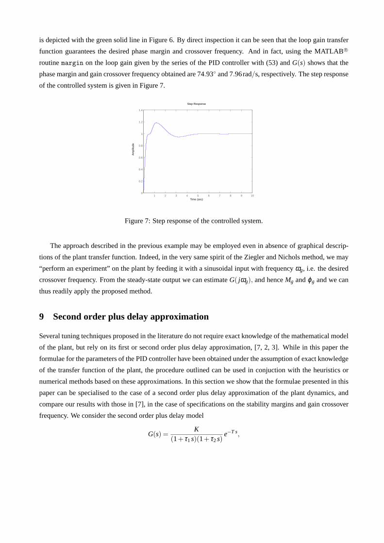
of the controlled system is given in Figure 7.
1 2 3 4 5 6 7 8 9 100
0.2
0.4
0.6
0.8
1
1.2
1.4
Step Response
Time (sec)
Am
plitu
de
Figure 7: Step response of the controlled system.
The approach described in the previous example may be employed even in absence of graphical descrip-
tions of the plant transfer function. Indeed, in the very same spirit of the Ziegler and Nichols method, we may
“perform an experiment” on the plant by feeding it with a sinusoidal input with frequencyωg, i.e. the desired
crossover frequency. From the steady-state output we can estimateG( jωg), and henceMg andϕg and we can
thus readily apply the proposed method.
9 Second order plus delay approximation
Several tuning techniques proposed in the literature do not require exact knowledge of the mathematical model
of the plant, but rely on its first or second order plus delay approximation,[7, 2, 3]. While in this paper the
formulae for the parameters of the PID controller have been obtained under the assumption of exact knowledge
of the transfer function of the plant, the procedure outlined can be used inconjuction with the heuristics or
numerical methods based on these approximations. In this section we show that the formulae presented in this
paper can be specialised to the case of a second order plus delay approximation of the plant dynamics, and
compare our results with those in [7], in the case of specifications on the stability margins and gain crossover
frequency. We consider the second order plus delay model
G(s) =K
(1+ τ1s)(1+ τ2s)e−T s,
whereτ1,τ2,T > 0 andK > 0. A direct calculation shows that
Mg =
√
(1+ω2g τ2
1)(1+ω2g τ2
1)
K,
ϕg = θ −π +arctan(ωg τ1)+arctan(ωg τ2),
whereθ = PM+ωgT, which lead to
Mg cos(ϕg) =ωg(τ1+ τ2) sinθ − (1−ω2
g τ1 τ2) cosθK
.
If the specifications are on the ratioσ = Td/Ti , the parameters of the compensator can be computed using
directly (12-14), that with this particular model yield
Kp =ωg(τ1+ τ2) sinθ − (1−ω2
g τ1 τ2) cosθK
,
Ti =(1−ω2
p τ1 τ2) tanθ +ωp(τ1+ τ2)
(1−ω2p τ1 τ2)−ωp(τ1+ τ2) tanθ
,
Td = Ti σ .
If the specifications are on both the phase and gain margin (and on the gain crossover frequency), we must also
compute
Mp =
√
(1+ω2p τ2
1)(1+ω2p τ2
1)
K,
ϕp = −π +ωpT +arctan(ωp τ1)+arctan(ωp τ2),
so that
Mp cos(ϕp) =ωp(τ1+ τ2) sin(ωpT)− (1−ω2
p τ1 τ2) cos(ωpT)
GM ⋅ K.
Therefore, in order to achieve the desired phase and gain margins at thedesired gain crossover frequency, we
need to find the rootsωp of the equation
ψ(ωp) = ωp(τ1+ τ2) sin(ωpT)− (1−ω2p τ1 τ2) cos(ωpT)−GM ⋅ K ⋅ Mg cos(ϕg) = 0. (54)
Notice that this time functionψ(ωp) is not polynomial, since the transfer function of the model is not rational.
The roots of this equation can be determined numerically, as shown in the following example. Of all the roots
of ψ(ωp), one satisfying the conditions of Theorem 3.2 must be determined (if no suchroots exist, the problem
does not admit solutions), and compute the parameters of the PID controller using (26-28).
Example 9.1 In this example we compare the results presented in this paper with those basedon a second
order approximation described in [7]. In particular, we consider the process in [7, Table 5] described by the
transfer function 1/(s+1)5 and approximated with the second order model
G(s) =e−1.73s
(1+1.89s)2 .
0 2 4 6 8 10−300
−250
−200
−150
−100
−50
0
50
100
150
200ψ(ωp)
ωp
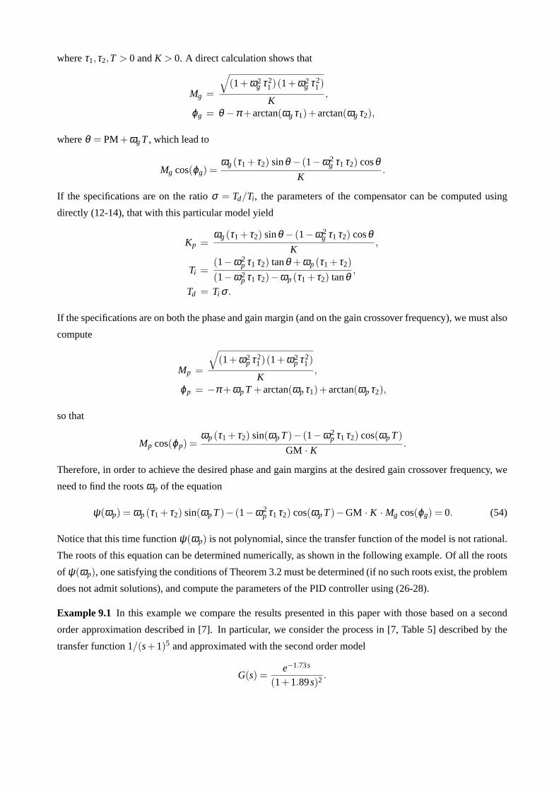
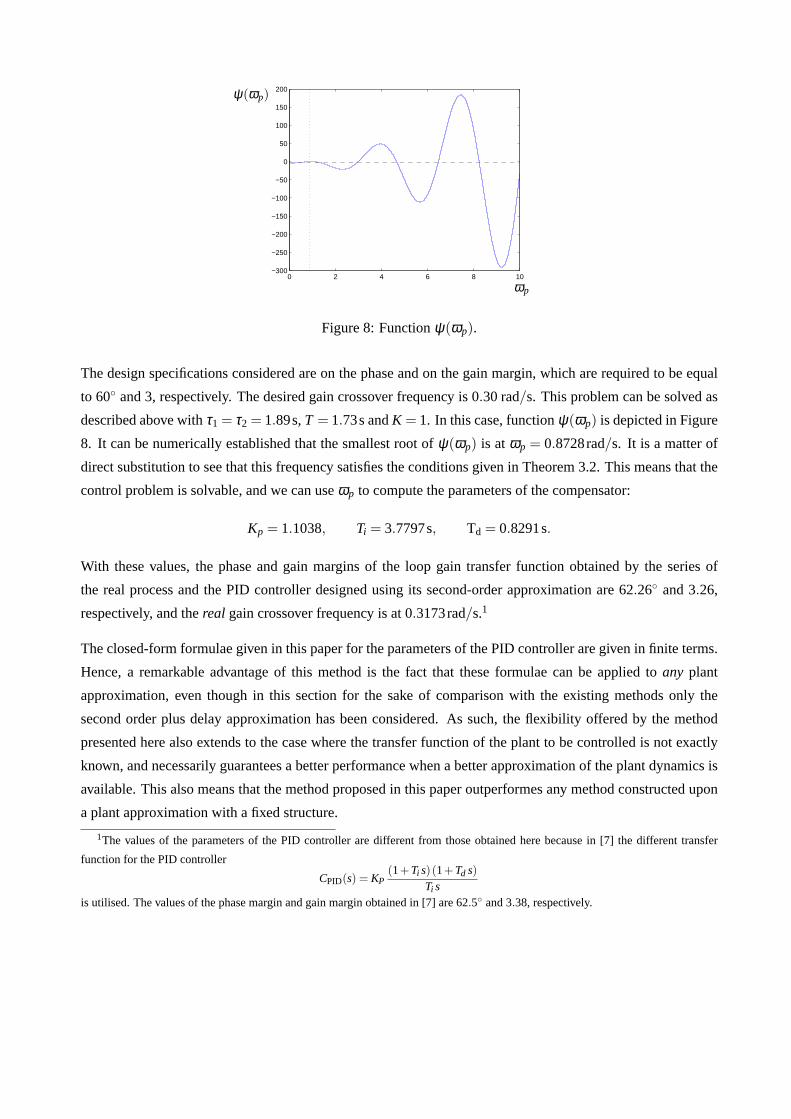
Figure 8: Functionψ(ωp).
The design specifications considered are on the phase and on the gain margin, which are required to be equal
to 60∘ and 3, respectively. The desired gain crossover frequency is 0.30 rad/s. This problem can be solved as
described above withτ1 = τ2 = 1.89s,T = 1.73s andK = 1. In this case, functionψ(ωp) is depicted in Figure
8. It can be numerically established that the smallest root ofψ(ωp) is atωp = 0.8728rad/s. It is a matter of
direct substitution to see that this frequency satisfies the conditions given inTheorem 3.2. This means that the
control problem is solvable, and we can useωp to compute the parameters of the compensator:
Kp = 1.1038, Ti = 3.7797s, Td = 0.8291s.
With these values, the phase and gain margins of the loop gain transfer function obtained by the series of
the real process and the PID controller designed using its second-order approximation are 62.26∘ and 3.26,
respectively, and thereal gain crossover frequency is at 0.3173rad/s.1
The closed-form formulae given in this paper for the parameters of the PID controller are given in finite terms.
Hence, a remarkable advantage of this method is the fact that these formulaecan be applied toany plant
approximation, even though in this section for the sake of comparison with the existing methods only the
second order plus delay approximation has been considered. As such,the flexibility offered by the method
presented here also extends to the case where the transfer function of the plant to be controlled is not exactly
known, and necessarily guarantees a better performance when a betterapproximation of the plant dynamics is
available. This also means that the method proposed in this paper outperformes any method constructed upon
a plant approximation with a fixed structure.
1The values of the parameters of the PID controller are different from those obtained here because in [7] the different transfer
function for the PID controller
CPID(s) = KP(1+Ti s)(1+Td s)
Ti sis utilised. The values of the phase margin and gain margin obtained in [7] are 62.5∘ and 3.38, respectively.
10 Conclusions
A unified approach has been presented that enable the parameters of PID, PI and PD controllers (with corre-
sponding approximations of the derivative action when needed) to be computed in finite terms given appro-
priate specifications expressed in terms of steady-state performance, phase/gain margins and gain crossover
frequency. The synthesis tools developed in this paper eliminate the need oftrial-and-error and heuristic pro-
cedures in frequency-response design, and therefore they undoubtedly outperforms the heuristic, trial-and-error
and graphic approaches proposed so far in the literature for the feedback control problem with specifications on
the steady-state performance and on the gain/phase margins, in the case ofperfect knowledge of the model of
the plant. When the plant model is not exactly known – as is often the case in practice – the present method can
still be fruitfully employed for the design of the PID controller. Indeed, the formulae delivering the controller
parameters only require the magnitude and the argument of the frequency response of the plant at the desired
crossover frequency. These data can be obtained graphically by direct inspection over any of the Nyquist, Bode
and Nichols diagrams (with the advantage that no special charts are needed). Alternatively, the closed-form
design techniques can be used jointly with a first or second order plus delay approximation of the plant to
deliver the desired values of the stability margins and crossover frequency.
References
[1] Charles L. Phillips. Analytical Bode Design of Controllers.IEEE Transactions on Education, E-28,
no. 1, pp. 43–44, 1985.
[2] K.J. Astrom, and T. Hagglund,PID Controllers: Theory, Design, and Tuning, second edition. Instrument
Society of America, Research Triangle Park, NC, 1995.
[3] K.J. Astrom, and T. Hagglund,Advanced PID Control. Instrument Society of America, Research Trian-
gle Park, NC, 2006.
[4] A. Datta, M.-T. Ho, and S.P. Bhattacharyya.Structure and Synthesis of PID Controllers. Springer, 2000.
[5] A. Ferrante, A. Lepschy, and U. Viaro.Introduzione ai Controlli Automatici. UTET Universit, 2000.
[6] G. Franklin, J.D. Powell, and A. Emami-Naeini .Feedback Control of Dynamic Systems. Prentice Hall,
2006.
[7] W.K. Ho, and C.C. Hang, and L.S. Cao, Tuning of PID Controllers Based on Gain and Phase Margin
Specifications.Automatica, vol. 31, no. 3, pp. 497–502, 1995.
[8] L.H. Keel and S.P. Bhattacharyya. Controller Synthesis Free of Analytical Models: Three Term Con-
trollers. IEEE Transactions on Automatic Control, AC-53, no. 6, pp. 1353–1369, 2008.
[9] K. Kim, and Y.C. Kim,, The Complete Set of PID Controllers with Guaranteed Gain and Phase Mar-
gins. Proceedings of the 44th IEEE Conference on Decision and Control, and the European Control
Conference 2005, pp. 6533–6538, Seville, Spain, December 12-15, 2005.
[10] G. Marro, TFI: Insegnare ed apprendere i controlli automatici di base con MATLABR⃝. Zanichelli Ed.,
Bologna (Italy), 1998.
[11] K. Ogata.Modern Control Engineering. 2nd edn. Prentice Hall, Englewood Cliffs, NJ, 2000.
[12] S. Skogestad. Simple analytic rules for model reduction and PID controller tuning. Journal of Process
Control, vol. 13, pp. 291-309, 2003.
[13] A. Visioli, Practical PID Control. Advances in Industrial Control, Springer-Verlag, 2006.
[14] W.R. Wakeland. Bode Compensation Design.IEEE Transactions on Automatic Control, AC-21, no. 5,
pp. 771–773, 1976.
[15] R. Zanasi and G. Marro, New formulae and graphics for compensator design.Proceedings of the 1998
IEEE International Conference on Control Applications, Vol. 1, pp. 129–133, 1-4 September 1998.
[16] K.S. Yeung, and K.H. Lee. A Universal Design Chart for LinearTime-Invariant Continuous-Time and
Discrete-Time Compensators.IEEE Transactions on Education, E-43, no. 3, pp. 309–315, 2000.
[17] R. Zanasi and R. Morselli, Discrete Inversion Formulas for the Design of Lead and Lag Discrete
Compensators.Proceedings of the European Control Conference 2009, pp. 5069–5074, August 23–26,
2009.
[18] J.G. Ziegler, and N.B. Nichols, Optimum settings for automatic controllers.Trans. ASME, vol. 64, pp.
759-768, 1942.