exact wkb analysis of n = 2 gauge theories wkb analysis of n= 2 gauge theories sujay k. ashoka;1,...
TRANSCRIPT

Exact WKB Analysis of N = 2 Gauge Theories
Sujay K. Ashoka,1, Dileep P. Jatkarb,2, Renjan R. Johna,3,
Madhusudhan Ramana,4, Jan Troostc,5
a Institute of Mathematical Sciences
C. I. T. Campus, Taramani
Chennai, India 600113
b Harish-Chandra Research Institute
Chhatnag Road, Jhusi,
Allahabad, India 211019
c Laboratoire de Physique Theorique
de l’Ecole Normale Superieure
CNRS
PSL Research University
Sorbonne Universites
75005 Paris, France
Abstract
We study N = 2 supersymmetric gauge theories with gauge group SU(2) coupled to funda-
mental flavours, covering all asymptotically free and conformal cases. We re-derive, from the
conformal field theory perspective, the differential equations satisfied by ε1- and ε2-deformed
instanton partition functions. We confirm their validity at leading order in ε2 via a saddle-point
analysis of the partition function. In the semi-classical limit we show that these differential
equations take a form amenable to exact WKB analysis. We compute the monodromy group
associated to the differential equations in terms of ε1-deformed and Borel resummed Seiberg-
Witten data. For each case, we study pairs of Stokes graphs that are related by flips and pops,
and show that the monodromy groups allow one to confirm the Stokes automorphisms that
arise as the phase of ε1 is varied. Finally, we relate the Borel resummed monodromies with the
traditional Seiberg-Witten variables in the semi-classical limit.
[email protected]@[email protected]@[email protected]
arX
iv:1
604.
0552
0v1
[he
p-th
] 1
9 A
pr 2
016

Contents
1 Introduction 2
2 The Conformal Field Theory Perspective 3
2.1 The Five-Point Block . . . . . . . . . . . . . . . . . . . . . . . . . . . . . . . . . . . . 4
2.2 The Null Vector Decoupling Equations for Irregular Blocks . . . . . . . . . . . . . . 5
2.3 The Semi-Classical Limit . . . . . . . . . . . . . . . . . . . . . . . . . . . . . . . . . 7
2.4 The Semi-Classical Irregular Blocks . . . . . . . . . . . . . . . . . . . . . . . . . . . . 7
3 The Exact WKB Analysis of Differential Equations 8
3.1 The Exact WKB Method . . . . . . . . . . . . . . . . . . . . . . . . . . . . . . . . . 9
3.2 The Applicability of the Exact WKB Analysis . . . . . . . . . . . . . . . . . . . . . . 15
3.3 Theorems on Stokes Automorphisms . . . . . . . . . . . . . . . . . . . . . . . . . . . 16
4 The Monodromy Group 17
4.1 Pure Super Yang-Mills . . . . . . . . . . . . . . . . . . . . . . . . . . . . . . . . . . . 18
4.2 One Flavour . . . . . . . . . . . . . . . . . . . . . . . . . . . . . . . . . . . . . . . . . 20
4.3 Two Flavours . . . . . . . . . . . . . . . . . . . . . . . . . . . . . . . . . . . . . . . . 22
4.4 Three Flavours . . . . . . . . . . . . . . . . . . . . . . . . . . . . . . . . . . . . . . . 25
4.5 The Conformal Theory . . . . . . . . . . . . . . . . . . . . . . . . . . . . . . . . . . . 27
5 The Gauge Theory Perspective 33
5.1 The Seiberg-Witten Variables . . . . . . . . . . . . . . . . . . . . . . . . . . . . . . . 34
5.2 The Non-Perturbative Prepotential . . . . . . . . . . . . . . . . . . . . . . . . . . . . 36
6 Conclusions 37
A The Null Vector Decoupling with Irregular Blocks 39
A.1 One Irregular Puncture . . . . . . . . . . . . . . . . . . . . . . . . . . . . . . . . . . 39
A.2 Two Irregular Punctures . . . . . . . . . . . . . . . . . . . . . . . . . . . . . . . . . . 40
B Stokes Graphs 42
B.1 The Double Flip . . . . . . . . . . . . . . . . . . . . . . . . . . . . . . . . . . . . . . 42
B.2 The Pop . . . . . . . . . . . . . . . . . . . . . . . . . . . . . . . . . . . . . . . . . . . 42
C The Saddle Point Analysis 42
C.1 Nf = 4 . . . . . . . . . . . . . . . . . . . . . . . . . . . . . . . . . . . . . . . . . . . . 46
C.2 Nf = 3 . . . . . . . . . . . . . . . . . . . . . . . . . . . . . . . . . . . . . . . . . . . . 46
C.3 Nf = 2: asymmetric realization . . . . . . . . . . . . . . . . . . . . . . . . . . . . . . 47
C.4 Nf = 2: symmetric realization . . . . . . . . . . . . . . . . . . . . . . . . . . . . . . . 48
C.5 Nf = 1 . . . . . . . . . . . . . . . . . . . . . . . . . . . . . . . . . . . . . . . . . . . . 48
C.6 Nf = 0 . . . . . . . . . . . . . . . . . . . . . . . . . . . . . . . . . . . . . . . . . . . . 49
1

1 Introduction
For some time now, we have been able to compute the low-energy effective action of N = 2 su-
persymmetric gauge theories in four dimensions. In [1, 2], the solution for the low-energy theory
was given in terms of an algebraic curve and an associated differential. Subsequent works have
simplified and clarified many aspects of the Seiberg-Witten solution. The Seiberg-Witten curves
may be intuitively pictured in terms of M-theory five-branes [3], and this geometric picture has
inspired a description of class S theories in terms of punctured Riemann surfaces [4]. In a paral-
lel development, it has also become possible to compute instanton contributions by invoking the
powerful machinery of equivariant localization [5]. Of particular note, the calculation of the gauge
theory partition function on S4 via localization naturally incorporates these instanton sums [6]. All
these developments were key to writing a dictionary between observables in four-dimensional gauge
theories and those in two-dimensional conformal field theories: the 2d/4d correspondence [7].
The 2d/4d correspondence makes it possible to use the technology of conformal field theory to
gain deeper insights into the behavior of N = 2 gauge theories. For instance, the Ω-deformed gauge
theory partition function with a surface operator insertion maps to the meromorphic solution of
a null vector decoupling equation [8, 9]. Thus, an analysis of conformal blocks in two-dimensional
conformal field theory yields information about surface operators in gauge theories. These con-
formal blocks can be viewed as solutions to Riemann-Hilbert problems specified by a differential
equation with singularities and associated monodromies [10]. We expect this exact picture to be
valid in gauge theory (and the field theory limit of topological string theory) [11].
In this paper, we study quantum chromodynamics with N = 2 supersymmetry and gauge group
SU(2), and the corresponding Virasoro conformal blocks. In particular, we study the differential
equation that the instanton partition function with surface operator insertion satisfies. This corre-
sponds to an analysis of null vector decoupling equations in the presence of irregular blocks. The
differential equations satisfied by correlators involving irregular blocks were described in [11–13].
The equations are exact in the Ω-deformation parameters (ε1, ε2), and provide for a map to standard
gauge theory expressions for the Seiberg-Witten curve, including εi corrections.
We then concentrate on the limit ε2/ε1 → 0 [14], which is a large central charge limit in the
conformal field theory. It has been shown in e.g. [15–17] that a WKB analysis of the null vector
decoupling equations in this semi-classical limit reproduces the non-convergent ε1-expansion of the
instanton partition function of the gauge theory.6 There is a rich literature [20–29] on methods
which may be used to enhance these results non-perturbatively. Using the exact WKB analysis, we
study the resulting differential equations satisfied by the (ir)regular conformal blocks (equivalently,
the ε1-deformed surface operator partition function). This allows us to compute the monodromy
group of each of the differential equations as a function of (i) the parameters of the differential
equations, and (ii) the Borel resummed monodromies that are properties of individual solutions.
The monodromy group contains information about the instanton partition function with surface
operator insertion, which is non-perturbative in ε1. In doing so, we provide the underlying exact
picture [10] with a detailed description of how these beautiful and abstract mathematical constructs
reduce to the more hands-on limiting analysis of N = 2 gauge theories to which we have become
6For non-perturbative results in the context of topological strings we refer to [18,19].
2

accustomed.
In this physical set-up, we apply the theorems of [29], thereby drawing on intuition from both
gauge theory and the mathematical study of singular perturbation theory [27]. As a by-product,
we add details to the WKB analysis and provide a calculation of the monodromy group of the dif-
ferential equation in terms of deformed gauge theory data. For instance, we analyze the occurrence
of a double flip, consisting of simultaneous single flips. Two different ways of splitting the double
flip into two single flips give the same monodromy group and Stokes automorphism. Although we
demonstrate this result in the context of Nf = 4 theory, this is a new result in the exact WKB
method and we believe it is valid in a more general context.
In [30], a WKB analysis of the Hitchin systems corresponding to circle compactifications of
undeformed SU(2) gauge theories was undertaken. Our work may be viewed as an alternative
route to the WKB analysis, which is closely related to [30] at zeroth order in ε1.
Our broader goal is to communicate the extreme generality of the correspondence between ε1-
deformed N = 2 gauge theories — specifically, their instanton partition functions with surface
operator insertions — and certain Schrodinger equations amenable to exact WKB analysis. As a
first step, we show the extent to which the program applied to pure N = 2 super Yang-Mills in [31]
generalizes to theories with matter.
We will now briefly present the structure of our paper. In section 2, we present a derivation
of the null vector decoupling equation satisfied by the five-point conformal block with a light
degenerate insertion, which has a null vector at level two. We apply the collision procedure of [32]
to produce irregular conformal blocks and derive the null vector decoupling equations satisfied
by the limit blocks. We then consider the semi-classical limit (of infinite central charge) of these
differential equations. These equations will be the starting point for the exact WKB analysis of
section 3. In this section, we briefly review the exact WKB approach, and in section 4 apply it to
the calculation of the monodromy groups of our differential equations. We make contact with the
standard undeformed Seiberg-Witten perspective in section 5 and end with comments and future
directions for work in section 6. The appendices collect details regarding the derivation of the
ε2-exact differential equations for the asymptotically free theories, and an independent check of the
semi-classical differential equations via the saddle-point analyses of Nekrasov partition functions
[34].
2 The Conformal Field Theory Perspective
In this section, we present the null vector decoupling equation satisfied by the five-point conformal
block with one degenerate operator insertion. We then list the corresponding equations satisfied
by irregular blocks that arise when punctures collide [32]. We study these equations within the
framework of conformal field theory, and finally, exploit the fact that these conformal blocks also
capture the εi-deformed instanton partition function of N = 2 supersymmetric gauge theories in
four dimensions with SU(2) gauge group and a varying number of flavours [5]. We thus lay the
groundwork for further analysis of these partition functions, which will be non-perturbative in the
deformation parameter ε1. For completeness, we provide the details of the derivation of all these
equations in appendix A.
3

We start our analysis by considering regular conformal blocks with four ordinary primary op-
erator insertions on the sphere and one degenerate operator insertion with a null vector at level
two, which remains light in the limit of large central charge. On the gauge theory side of the 2d/4d
correspondence, this set-up corresponds to the conformal Nf = 4 case. To get asymptotically free
(lower Nf ) theories, we sequentially collide primary operators on the sphere in such a way that
they generate irregular conformal blocks [32]. The case of three flavours will correspond to one
irregular block, the case of two flavours can correspond to either one or two irregular blocks, while
a lower number of flavours corresponds to two irregular blocks in the conformal field theory. For
all these collision limits, we give the corresponding null vector decoupling equations.
2.1 The Five-Point Block
We study a conformal field theory with central charge
c = 1 + 6Q2 , where Q = b+ b−1 and b =
√ε2ε1. (2.1)
We consider a five-point chiral conformal block Ψ with four primary operator insertions Vαi and
an insertion of a degenerate field Φ2,1(z) of the Virasoro algebra [9]:
Ψ(zi, z) =⟨
Φ2,1(z) :4∏i=1
Vαi(zi) :⟩. (2.2)
The degenerate field Φ2,1 has conformal dimension ∆2,1
∆2,1 = −1
2− 3
4
ε2ε1, (2.3)
while the conformal dimensions of the generic primaries are denoted ∆αi . We have chosen the
degenerate insertion such that it remains light in the limit of large central charge ε2/ε1 → 0.
The degenerate field Φ2,1 has a null vector at level two, and consequently satisfies the null vector
conditionε1ε2∂2Φ2,1(z)+ :T (z)Φ2,1(z) : = 0 , (2.4)
where the operator T (z) is the holomorphic stress tensor of the conformal field theory. Using the
operator product expansion between the stress tensor and the primary fields, the second term can
be written as:⟨:T (z)Φ2,1(z) :
4∏i=1
Vαi(zi)⟩
=4∑i=1
(∆αi
(z − zi)2+
1
z − zi∂
∂zi
) ⟨Φ2,1(z)
4∏i=1
Vαi(zi)⟩. (2.5)
Imposing global conformal invariance allows us to express the derivatives with respect to z1, z3 and
z4 in terms of the derivatives at z2 and z. Then, setting the insertions to be at (z, 0, q, 1,∞), the
null vector decoupling equation takes the form[ε1ε2
∂2
∂z2+
(∆α2
(z − q)2+
q(q − 1)
z(z − 1)(z − q)∂
∂q
)− 2z − 1
z(z − 1)
∂
∂z+
∆α1
z2+
∆α3
(z − 1)2
−∆2,1 + ∆α1 + ∆α2 + ∆α3 −∆α4
z(z − 1)
]Ψ(z, q) = 0 (2.6)
4

The null vector decoupling on the five point conformal block was also studied in [9, 33]. The
conformal dimensions ∆i of the primary fields Vαi can be written in terms of the momenta αi as
∆αi = αi(Q− αi) . (2.7)
We further parameterize the momenta αi in terms of the four masses mi:
α1 =Q
2+m1 −m2
2√ε1ε2
, α2 =Q
2+m1 +m2
2√ε1ε2
,
α3 =Q
2− m3 +m4
2√ε1ε2
, α4 =Q
2− m3 −m4
2√ε1ε2
.
(2.8)
As a function of the masses, the conformal dimensions are
∆α1 =(ε1 + ε2)2 − (m1 −m2)2
4ε1ε2, ∆α2 =
(ε1 + ε2)2 − (m1 +m2)2
4ε1ε2,
∆α3 =(ε1 + ε2)2 − (m3 +m4)2
4ε1ε2, ∆α4 =
(ε1 + ε2)2 − (m3 −m4)2
4ε1ε2.
(2.9)
In terms of these variables that are appropriate for comparison to the four dimensional gauge
theory, the null vector decoupling equation for the Nf = 4 theory takes the following form:
[−ε21
∂2
∂z2+
(m1 −m2)2
4z2+
(m1 +m2)2
4(z − q)2+
(m3 +m4)2
4(z − 1)2+m2
1 +m22 + 2m3m4
2z(1− z)
− ε21
(q2 − 2qz + z2
(z2 − 2z + 2
)4(z − 1)2z2(q − z)2
)+ ε1ε2
(q(1− q)
z(z − 1)(z − q)∂
∂q+
2z − 1
z(z − 1)
∂
∂z
+q2(−z2 + z − 1
)+ 2qz
(z2 − z + 1
)+ z2
(−2z2 + 3z − 2
)2(z − 1)2z2(q − z)2
)
+ε22
(q2(−3z2 + 3z − 1
)+ 2qz
(3z2 − 3z + 1
)+ z2
(−4z2 + 5z − 2
)4(z − 1)2z2(q − z)2
)]Ψ(z, q) = 0 . (2.10)
2.2 The Null Vector Decoupling Equations for Irregular Blocks
We now take limits of the five-point null vector decoupling equation (2.6) in which various primary
operators Vαi collide to form irregular conformal blocks of order one [32]. These limiting configu-
rations are in direct correspondence with the εi-deformed SU(2) gauge theories with Nf < 4. We
list below the null vector decoupling equations for each of these cases and refer to appendix A for
a detailed derivation. A summary of these equations can also be found in [11].
Nf = 3 : In this case, we have one irregular block of order one with a fourth order pole at z = 0.
In the gauge theory variables, we take q → 0 and m2 →∞, keeping the dynamical scale Λ3 = q m2
finite. The resulting differential equation is:
5

[−ε21
∂2
∂z2+
(m3 +m4)2
4(z − 1)2+
m3m4
z(1− z)+m1Λ3
z3+
Λ23
4z4+ ε1ε2
(1− 2z
z (1− z)∂
∂z+
1− 2z
2z(z − 1)2
)+
1
z2 (1− z)
(−ε1ε2Λ3
∂
∂Λ3+m2
1 +m1(ε1 + ε2)
)− ε21
4(z − 1)2+ ε22
(3− 4z)
4z(z − 1)2
]Ψ3(z,Λ3) = 0 .
Nf = 2 : There are two ways to reach the case with two flavours from the case with three flavours.
One could decouple either the flavour with mass m1 or one of those with masses m3,4. As shown
in [30], these lead to inequivalent Hitchin systems and give rise to distinct differential equations.
Let us first consider the irregular block of order one with a third order pole at z = 0. This
corresponds to decoupling m1. We refer to this as the asymmetric configuration and the associated
null vector decoupling equation becomes:[−ε21
∂2
∂z2+
(m3 +m4)2
4(z − 1)2+
m3m4
z(1− z)+
Λ22
z3− ε1ε2
2z2(1− z)Λ2
∂
∂Λ2
+ε1ε2
(1− 2z
z(1− z)∂
∂z+
1− 2z
2z(z − 1)2
)− ε21
4(z − 1)2+ ε22
(3− 4z)
4z(z − 1)2
]Ψ2,A(z,Λ2) = 0 (2.11)
Alternatively, one can consider two irregular blocks of order one, with equal fourth order poles.
This corresponds to decoupling m3 while keeping m1 and m4 finite. We refer to this as the sym-
metric configuration and the associated null vector decoupling equation reads:
[−ε21
∂2
∂z2+
Λ22
4z4+
Λ2m1
z3(z − 1)2− Λ2m4
z(z − 1)3+
Λ22
4(z − 1)4+
2− 3z
4z(z − 1)2(2ε1ε2 + 3ε22)
+1
z2(z − 1)2
(−ε1ε2Λ2
∂
∂Λ2− 2Λ2m1 +m2
1 +m1(ε1 + ε2)
)+ ε1ε2
3z − 1
z(z − 1)
∂
∂z
]Ψ2,S(z,Λ2) = 0 .
Nf = 1 : We consider two irregular blocks of order one with one fourth order pole and one third
order pole. This corresponds to decoupling m4 and the null vector decoupling equation takes the
form
[− ε21
∂2
∂z2+
Λ21
4z4+
Λ1m1
z3(z − 1)2− Λ2
1
4z(z − 1)3+
2− 3z
4z(z − 1)2(2ε1ε2 + 3ε22) + ε1ε2
3z − 1
z(z − 1)
∂
∂z
+1
z2(z − 1)2(−ε1ε2Λ1
∂
∂Λ1− 2Λ1m1 +m2
1 +m1(ε1 + ε2))
]Ψ1(z,Λ1) = 0 . (2.12)
Nf = 0 : Finally, we consider the case with two irregular blocks of order one with equal third
order poles. All masses have been decoupled and the null vector decoupling equation becomes[−ε21
∂2
∂z2+
Λ20
z3(z − 1)2+
1
z2(z − 1)2
(−1
2ε1ε2Λ0
∂
∂Λ0− 2Λ2
0
)+
Λ20
z(z − 1)3
+ε1ε23z − 1
z(z − 1)
∂
∂z+
2− 3z
4z(z − 1)2(2ε1ε2 + 3ε22)
]Ψ0(z,Λ0) = 0 . (2.13)
This completes the list of six differential equations that we refer to throughout.
6

2.3 The Semi-Classical Limit
In the rest of our paper, we will concentrate on the limit ε2/ε1 → 0, which is a large central charge
limit. We keep the ratio of the mass parameters mi and the deformation parameter ε1 fixed. In
this limit, the primary insertions Vαi are heavy, while the degenerate insertion Φ2,1 is light. Thus,
in this limit, the differential equation (2.6) simplifies, and we can drop the term proportional to ∂z,
while the terms proportional to the conformal dimensions ∆αi grow large. To simplify the equation
further, we must specify the leading dependence of the q-derivative of the five-point block on ε2.
To that end, we make the semi-classical ε2 → 0 ansatz
Ψ(z, q) = exp
(− F (q,mi, εi)
ε1ε2
)ψ(z, q) . (2.14)
We suppose that the q-derivative of the remaining function ψ(z, q) is sub-dominant in the small
ε2/ε1 limit, and observe that the leading dependence in ε2 is only on the cross-ratio q of the heavy
operators. We then define the quantity
u = q(1− q)∂qF . (2.15)
The parameter u is identified with the Coulomb modulus of the gauge theory up to shifts that
depend on the masses. Substituting this parameterization into the null vector decoupling equation
and taking the semi-classical limit ε2 → 0 leads to the Schrodinger equation(−ε21
d2
dz2+Q(z, ε1)
)ψ(z, q) = 0 , (2.16)
where the potential function Q has an ε1 expansion which terminates at second order
Q(z) = Q0(z) + ε1 Q1(z) + ε21 Q2(z) . (2.17)
The coefficient functions are
Q0(z) = − u
z(z − 1)(z − q)+
(m1 −m2)2
4z2+
(m1 +m2)2
4(z − q)2+
(m3 +m4)2
4(z − 1)2+m2
1 +m22 + 2m3m4
2z(1− z),
Q1(z) = 0 ,
Q2(z) = − 1
4z2− 1
4(z − 1)2− 1
4(z − q)2+
1
2z(z − 1).
(2.18)
2.4 The Semi-Classical Irregular Blocks
The same type of ansatz (2.14) can be used in order to obtain the differential equations for the
irregular blocks in the semi-classical ε2 → 0 limit. The variable parameterizing the Coulomb
modulus is now defined as
u = ΛNf∂F
∂ΛNf, (2.19)
7

where ΛNf is the corresponding strong coupling scale of the Nf < 4 gauge theory. As in the
conformal case, the prepotential of the gauge theory will differ mildly from F . However, what is
of importance to us is the pole structure of the functions Qk(z), and we choose a parameterization
that descends naturally from the conformal theory and that allows for a simple presentation of the
differential equations. In the following, we present all the asymptotically free cases:
• Nf = 3: The Schrodinger equation which governs the ε1-deformed gauge theory is given by[−ε21
∂2
∂z2+
(m3 +m4)2
4(z − 1)2+
m3m4
z(1− z)+m1Λ3
z3+
Λ23
4z4+
u
z2(1− z)− ε21
4(z − 1)2
]ψ3(z,Λ3) = 0 .
(2.20)
• Nf = 2 (asymmetric realization): The differential equation in the semi-classical limit takes
the form[−ε21
∂2
∂z2+
(m3 +m4)2
4(z − 1)2+
m3m4
z(1− z)+
Λ22
z3+
u
z2(1− z)− ε21
4(z − 1)2
]ψ2,A(z,Λ2) = 0 (2.21)
• Nf = 2 (symmetric realization):[−ε21
∂2
∂z2+
Λ22
4z4+
Λ2m1
z3(z − 1)2− Λ2m4
z(z − 1)3+
Λ22
4(z − 1)4+
u
z2(z − 1)2
]ψ2,S(z,Λ2) = 0 .
(2.22)
• Nf = 1:[−ε21
∂2
∂z2+
Λ21
4z4+
Λ1m1
z3(z − 1)2− Λ2
1
4z(z − 1)3+
u
z2(z − 1)2
]ψ1(z,Λ1) = 0 . (2.23)
• Nf = 0: Finally, for the pure super Yang-Mills theory, the equation reads[−ε21
∂2
∂z2+
Λ20
z3(z − 1)2+
u
z2(z − 1)2+
Λ20
z(z − 1)3
]ψ0(z,Λ0) = 0 . (2.24)
We have thus obtained the differential equations which we analyze in detail in section 4.
3 The Exact WKB Analysis of Differential Equations
In this section, we review the exact WKB approach to the analysis of differential equations and
apply it to the null vector decoupling equations in the semi-classical limit. We will carry out the
exact WKB analysis with respect to the small parameter ε1. Our analysis will therefore be valid
to zeroth order in ε2 and non-perturbatively in ε1. Below, we briefly review the salient features of
the exact WKB analysis and refer the reader to [27,29] for a more comprehensive treatment of the
same.
8

3.1 The Exact WKB Method
The differential equations that we study can be written in the form of a Schrodinger equation:(−ε21
d2
dx2+Q(x)
)ψ(x, ε1) = 0 . (3.1)
We allow the function Q to have an expansion of the form
Q(x) = Q0(x) + ε1 Q1(x) + ε21 Q2(x) + · · · . (3.2)
For the null vector decoupling equations that we study, the only non-zero coefficient functions are
Q0, Q1 and Q2. We choose a WKB ansatz for the solution to this differential equation, which takes
the form
ψ(x, ε1) = exp
(∫ x
x0
dx′ S(x′, ε1)
), (3.3)
with S(x, ε1) expanded as a formal power series in ε1 as
S(x, ε1) =1
ε1S−1(x) + S0(x) + ε1 S1(x) + · · · . (3.4)
Substituting this ansatz into the differential equation, we get recursion relations governing the
coefficients Sk
S2−1 = Q0 , (3.5)
2S−1Sn+1 +∑k+l=n
SkSl +dSndx
= Qn+2 for n ≥ −1 . (3.6)
We see that the initial conditions governing the system of recursion relations allow for two possible
sets of solutions to these recursion relations, as S−1 = ±√Q0. We also note the crucial feature that
the zeroes of Q0, which we call turning points, introduce branch cuts on the Riemann surface Σ
on which our differential equation and its exact solutions live. Thus, in our exact WKB treatment,
we introduce a new manifold Σ, which is a double cover of the Riemann surface, and we move
between sheets as we pass branch cuts that emanate from turning points, or odd order poles. From
hereon, we will distinguish the choice of WKB solution by attaching to it the subscript (±). We
also observe that in the ε1-expansion of S(x, ε1), the sets of odd and even coefficients are dependent.
If we define
Sodd =∑j≥0
S2j−1 ε2j−11 and Seven =
∑j≥0
S2j ε2j1 , (3.7)
we have the relation
Seven = −1
2
d
dxlogSodd . (3.8)
Putting all this together, we can write down a formal expression for the two linearly independent
solutions to our differential equation:
ψ± =1√Sodd
exp
±∫ x
x0
dx′ Sodd
. (3.9)
9

This formal expression should be understood as an analytic function of x multiplying an asymptotic
series in ε1 :
ψ± = exp
± 1
ε1
∫ x
x0
dx′√Q0(x′)
ε1/21
∞∑k=0
εk1 ψ±,k(x) . (3.10)
Borel Resummation
In the exact WKB approach, it is convenient to normalize wave-functions at distinguished points
of the differential equation. As mentioned earlier, in addition to the singularities of the coefficient
functions of the differential equations, their zeros (turning points) also play an important role. We
will normalize our solutions with respect to the turning points, i.e. choose the starting point x0 of
the integration path to be a turning point t,
ψ± =1√Sodd
exp
±∫ x
tdx′ Sodd
. (3.11)
Formal WKB solutions are generically divergent. To remedy this, we invoke Borel resummation:
a technique that constructs an analytic function whose asymptotic expansion matches the formal
WKB series. The Borel transformed series is defined as
ψ(ε1) =
∞∑k=0
ψk εk1
Borel transform−−−−−−−−−→ ψ(y) =
∞∑k=1
ψkyk−1
(k − 1)!. (3.12)
Next, define the function [29]
Ψ(ε1) = ψ0 +
∫`θ
dy e−y/ε1ψ(y) , (3.13)
where `θ is the line connecting a point at which the series ψ(y) converges7 — typically, a turning
point — to the point at infinity at an angle θ. If this integral exists, Ψ(ε1) is the requisite analytic
function, called the Borel sum.
Notice that the Borel sum contains an angular dependence. In order to understand this better,
one must appreciate that Borel sums are typically defined only in regions of the complex ε1-plane,
and not throughout. These regions are bounded by Stokes lines, defined by the condition
Im
[∫ x
x0
dx′√Q0(x′)
]= 0 , (3.14)
and different Stokes regions are assigned different linear combinations of a given basis of analytic
solutions to the differential equation, arrived at via Borel resummation. One of the key components
of the exact WKB analysis is understanding how solutions in different Stokes regions are related by
analytic continuation; these often go by the name of “connection formulae”. However, before we
7To be precise, this is true for Gevrey-1 series, which in our context corresponds to the following statement. If
ψk is the kth coefficient of the asymptotic series then the series is Gevrey-1 type if growth of ψk is bounded by
ψk ≤ ABkk! for some constants A and B. If ψk is a function of a continuous variable, say, x ∈ C then this condition
applies to the supremum of ψk(x) in a compact subset of C.
10
address this transition behaviour, we will find it necessary to endow Stokes lines with an orientation.
To this end, we adopt the convention that Stokes lines are oriented away (i.e. the arrow on the
Stokes line is pointing away from a turning point) if
Re
[∫ x
x0
dx′√Q0(x′)
]> 0 (3.15)
along the Stokes line. Else, the arrow points towards the turning point.
Three Stokes lines emanate from a first order zero of Q0(x), which is also referred to as a simple
turning point. Thus one end of any Stokes line is at a turning point. The other end can either be
at a singularity or at a turning point. When both the end points of a Stokes line in a given Stokes
graph terminate at turning points then the corresponding Stokes graph is called “critical”.8
Connection Formulae
We are now in a position to state the connection formulae. For a Stokes graph which is not critical,
consider two regions U1 and U2 separated by a Stokes curve Γ, and consider Ψj± to be the Borel
sums of WKB solutions in each of the regions Uj . The connection formulae for the Borel sums in
different Stokes domains are given by:
if Re
[∫ x
x0
dx′√Q0(x′)
]< 0 on Γ :
Ψ1
+ = Ψ2+ ,
Ψ1− = Ψ2
− ± iΨ2+ ,
(3.16)
if Re
[∫ x
x0
dx′√Q0(x′)
]> 0 on Γ :
Ψ1
+ = Ψ2+ ± iΨ2
− ,
Ψ1− = Ψ2
− .(3.17)
In the above connection formulae, there is an ambiguity (±) that is fixed by noting that the turning
point that Γ originates from serves as a point of reference. If the path of analytic continuation
crosses Γ counter-clockwise as seen from the turning point, we pick the (+) sign, and if this path
crosses Γ clockwise, we pick the (−) sign. Later in this section, we will write down the Stokes
matrices that multiply wave-functions; these are equivalent to the above result.
The global properties of solutions to the differential equations we consider are governed by the
monodromy group and the Stokes phenomena around singular points. The monodromy group of
these differential equations can be expressed entirely in terms of two sets of quantities: (a) the
characteristic exponents at each singular point sk, and (b) the contour integrals of Sodd around
branch cuts. We now parameterize the characteristic exponents conveniently.
As a system of solutions to our differential equation, we consider the WKB solutions (3.9), and
define the characteristic exponents as residues of the differential:
Mk = Res√Q0(x)
∣∣∣x=sk
. (3.18)
8The general behaviour of Stokes lines is discussed in [29]. We restrict ourselves to situations that are relevant in
this work.
11

From the null vector decoupling equations we derived in the previous section, one can check that
the residues Mk are linear combinations of the mass parameters of the gauge theory. As the
monodromy group computations will use WKB wave-functions (3.9), we relate the residues of Sodd
to our characteristic exponents as9
Res Sodd(x, ε)∣∣∣x=sk
=Mk
ε1
√1 +
ε214M2
k
. (3.19)
Finally, upon exponentiating this contribution, we get the multiplier that affects WKB wave-
functions:
ν±k = exp
[iπ
(1±
√4M2
k
ε21+ 1
)]. (3.20)
Notice that ν+k = 1/ν−k , a fact that we will use repeatedly. Since the base point x0 will not always be
a turning point, the modified connection formulae can be obtained by a composition of the contour
integrals. We find it convenient to use a matrix notation to exhibit the connection formulae. As an
example, let us consider analytically continuing the Borel resummed wave-functions from Stokes
region U1 to Stokes region U2. As shown in figure 1, there are two distinct possibilities. If the
(A) (B)
Figure 1: Analytic continuation of wave-functions from U1 to U2
contour crosses a Stokes line that is directed inwards to a turning point as in figure 1 (A), we find
the connection formula: (Ψ1
+ , Ψ1−
)=⇒
(Ψ2
+ , Ψ2−
)(1 ±iu−1i
0 1
). (3.21)
In the above equation, we use the notation,
uj = exp
(2
∫γj
dx Sodd
), (3.22)
where γj is an oriented curve from the base point to the turning point tj . Along a contour that
crosses a Stokes line which is directed outwards from a turning point as in figure 1 (B), we have
9This is true under the assumptions that Re Mk 6= 0.
12

the connection formula: (Ψ1
+ , Ψ1−
)=⇒
(Ψ2
+ , Ψ2−
)( 1 0
±iui 1
). (3.23)
In the above, the +(−) sign is chosen for counter-clockwise (clockwise) crossing of the contour from
one Stokes region to the other, with respect to the turning point. For more complicated contours, it
is important to take into account contributions from any branch cuts and/or singularities enclosed
along the closed contour from the base point to the intersection point, the turning point and then
back to the base point. As a simple example of this phenomenon, let us suppose the contour chosen
happens to encircle a branch cut — say between tj and ti as in figure 2 – counter-clockwise. Here,
Figure 2: Encircling branch cuts
the curves γi are those that define the parameter ui. The closed contour γji that encircles the
branch cut has a contribution of the form
uji = exp
(∫γji
dx′ Sodd
), (3.24)
where from the figure it is clear that
uji = u−1j ui . (3.25)
One can see that although the ui by itself is dependent on the base point, the contour integral is
independent of this choice.
Contour Encircling a Turning Point
Let us make another important preliminary point regarding the choice of cycles. In order to define
the monodromy group, we first choose a base point and define a basis of closed loops that encircle
just the singularities. In some of the cases we encounter, there are branch cuts between turning
points and singularities. In such cases, we choose the contours to also include these turning points.
In order to prove that this is consistent with the usual definition of the monodromy group, let
us consider a contour that only encircles the turning point, as shown in figure 3.
13

Figure 3: Contour with base point x0 encircling a turning point t
If we choose to normalize the wave-functions at x0, the wave-functions undergo the following
transformation as we travel along the path:
Mx0,path =
(1 0iu1
1
)(0 −i
−i 0
)(1 0
iu1 1
)(1 iu1
0 1
)(3.26)
=
(u1 0
0 1u1
)(3.27)
Here we have associated the matrix −iσ1 to the branch-cut crossing, which ensures that we remain
on the same sheet of the Riemann surface. It can be easily shown that for any base point that one
may choose, the answer is trivial as above. If we chose the turning point itself to be the base-point,
u1 = 1 and the matrix reduces to the identity matrix. Since the net result is simply the identity
matrix, in order to calculate the monodromy matrix for the contour that encircles the singularity s,
one may just as well compute the monodromy of the wave-functions around the cycle that encircles
both the turning point t and the singularity s. We will make use of this repeatedly in those cases
in which the branch cut extends between a turning point and a singularity.
It is instructive to square this situation with the solution of a differential equation near an
ordinary point. It is known that any solution of a differential equation can be written as a Taylor
series in the neighbourhood of an ordinary point. The radius of convergence of this solution is
at least as much as the distance from the chosen point to the nearest singularity. The Taylor
series solution will clearly have trivial monodromy property. Although the WKB analysis assigns
a special status to turning points, from the differential equation point of view the turning point is
an ordinary point. Clearly, the branch cut and the Stokes lines emanating from a turning point are
artefacts of the WKB approximation and the insertion of the matrix −iσ1 restores the fact that
the turning point is an ordinary point of the differential equation.
Contours Encircling a Singular Point
Let us now consider the toy example, as shown in figure 4, where the contour encloses a singularity.10
10This example will illustrate the manner in which the Stokes matrices at each intersection are written down. The
Stokes lines here don’t end at turning points or singularities; the reader is encouraged to think of the figure as a part
14

Figure 4: Evaluation of Stokes matrices: effect of singularities
In figure 4, at the first intersection point A, the contour crosses counter-clockwise a Stokes line
emanating from ti. Thus, the Stokes matrix is(1 0
+iui 0
). (3.28)
In order to determine the Stokes matrix at B, we need to know to which turning point the Stokes
line is connected. Since this is irrelevant to the present discussion, we move on to consider the third
intersection point C. This time the contour crosses a Stokes line going into ti, and the crossing is
clockwise as seen from ti. Further, when this contour is completed using γj , we see that a singularity
is encircled counter-clockwise. Taking this into account, the Stokes matrix is(1 −iu−1
i ν−2k
0 1
). (3.29)
Finally, at the fourth intersection point D, the contour crosses the Stokes line clockwise. In fact, it is
very similar to the first intersection, except that now there is a singularity encircled. Consequently,
the Stokes matrix is (1 0
−iujν2k 0
). (3.30)
This concludes our brief review of the exact WKB analysis. We refer the reader to [27, 29] for a
more detailed discussion and further references.
3.2 The Applicability of the Exact WKB Analysis
The application of the exact WKB techniques depends on the precise differential equation under
consideration. Before we apply the exact WKB method to the equations derived in the previous
section, it is important to point out the subtleties in the applicability of this analysis. In the
Schrodinger type differential equations listed in sections 2.3 and 2.4, the parameter ε1 functions
as the Planck’s constant ~ in the WKB approximation scheme. For our null vector decoupling
equations, the potential has zeroth, first and second order terms in ε1. In order to apply the
of a complete Stokes graph that has been zoomed into.
15

exact WKB techniques to the solution of the differential equation, the ε1-deformed potential must
satisfy certain conditions. These consistency conditions not only ensure normalizability of the
wave-functions at singularities but also are useful in proving Borel summability of the WKB wave-
functions.
The necessary conditions (eq. (2.8) and (2.9) in [29]) are:
• If the leading coefficient Q0 has a pole of order m ≥ 3, then the order of Qn≥1 at that pole
should be smaller than 1 +m/2.
• If the pole of Q0 (at, say z = z0) is of order m = 2, then Qn 6=2 may have at most a simple
pole there and Q2 should have a double pole :
Q2 = − 1
4(z − z0)2(1 +O(z − z0)) as z → z. (3.31)
It is easily checked that the potentials that appear in the various Schrodinger type differential
equations in sections 2.3 and 2.4 satisfy these conditions.
3.3 Theorems on Stokes Automorphisms
Since all the equations listed in sections 2.3 and 2.4 satisfy the necessary conditions, the theorems
proved in [29] using these conditions can be directly applied to our equations. There is however,
an interesting exception and we will comment on it momentarily. In particular, the results of [29]
include theorems on the Stokes automorphisms that relate WKB resummed monodromies with a
given Borel resummation angle, to monodromies with another Borel resummation angle.
We will now list the relevant results from these theorems. Consider a closed curve γ on the
double cover Σ of the Riemann surface Σ encircling either a singularity or a turning point. We
then define the Voros symbol eVγ as a formal power series using the integral
Vγ(ε1) =
∮γdz Sodd(z, ε1) . (3.32)
The Borel sums of the Voros symbol are then defined as S±[eVγ ]. They satisfy the Stokes automor-
phism formula
S−[eVγ ] = S+[eVγ ](1 + S+[eVγ0 ])−(γ0,γ) (3.33)
whereby we suppose a simple flip, with the critical Stokes cycle being denoted by γ0, and (γ0, γ)
is the intersection number of the critical cycle with the cycle γ defining the Voros symbol. The
resummations S± are the Borel resummations of the Voros symbol on either side of (and close
enough to) the critical graph. The intersection numbers are defined using the convention that, if
the cycle γ1 has the arrow pointing outwards in the positive x direction and the cycle γ2, which
crosses γ1, with the arrow pointing towards the upper half-plane, then (γ1, γ2) = +1. When we have
Borel sums on either side of a pop rather than a flip, the Voros symbols (importantly, associated
to closed cycles) are trivially related
S−[eVγ ] = S+[eVγ ] . (3.34)
16

These two theorems govern the transformation of Voros symbols associated to closed cycles. In
the next section we will frequently use results of these theorems to study global properties of our
differential equations.
In the case of the conformal SU(2) gauge theory (with Nf = 4 flavours) however, the extra
assumptions of [29] are not always fully satisfied. In particular, in this case we find that pairs of
Stokes graphs that are related by a simultaneous or double flip, excluded in [29]. When such a
double flip occurs, we show that the formulae for the Stokes automorphisms derived for single flips
compose without change to give the Stokes automorphism for the double flip. This is an extension
of the results of [29]. We will discuss this case in detail in the next section.
4 The Monodromy Group
In this section, we study global properties of the differential equations derived in section 2. The
differential equations are second order and hence have two linearly independent global solutions.
The solutions undergo a monodromy as we analytically continue them around a singular point.
The monodromies, defined up to a change of basis, form a group called the monodromy group. The
monodromy group of the differential equations we consider can be expressed entirely in terms of
two sets of quantities: (i) the characteristic exponents νk at the singular points sk and (ii) the Borel
resummed contour integrals of the WKB differential Sodd around branch cuts, which we denote by
uij .
The connection formulae which relate the Borel resummed wave functions in the various Stokes
regions are sufficient to completely determine the monodromy group associated to the relevant null
vector decoupling equation. The Borel resummed exact WKB contour integrals depend on the
Borel resummation angle, (equivalently, on the phase of ε1) and undergo Stokes automorphisms
as a function of these parameters. Thus, the expression of the monodromy group in terms of the
resummed integrals varies, and we determine the explicit transformation rules as we pass through
a critical graph. In this section, we calculate the monodromy groups, starting with the simplest
case of zero flavours, with no regular singular points in the differential equation, and we end with
the conformal case (Nf = 4) which has four regular singular points.
We stress the fact that there is a dictionary between the Borel resummation angle θ, and
the phase of the zeroth order differential which is determined by the phase of ε1 in our set-up.
(See e.g. [29] for the details, which follow from the definition of the Borel sum.) We see that this
dictionary is given a natural home in ε1-deformed N = 2 gauge theories. The formal dependence on
the Borel resummation angle that induces the Stokes automorphism, has a physical counterpart in
the dependence of all non-perturbatively resummed monodromies on the phase of the deformation
parameter ε1.
A Brief Summary of our Analysis
Throughout this section, we perform the calculation of the monodromy group in a strong coupling
regime. In all the examples, we will plot the Stokes graphs emphasizing the connectivity of the
graphs and the choice of branch cuts; we refer to [30] for various possible sequences of Stokes
17
graphs. To illustrate the detailed coding of the monodromy group in terms of the characteristic
exponents and the resummed monodromies, as well as the ambiguity of their formal expression in
terms of the monodromies, we calculate the monodromy groups associated to two distinct Stokes
graphs. Equating the invariants constructed from the monodromy groups of the two graphs gives
us the Stokes automorphism relating the variables in each description. We will thus find concrete
descriptions of the monodromy group, as well as the Stokes automorphisms that the exact WKB
parameters undergo. The Stokes automorphisms must satisfy the theorems of [29] and this fact
serves as a consistency check of our analysis.
4.1 Pure Super Yang-Mills
The semi-classical null vector decoupling equation corresponding to the case of pure super Yang-
Mills theory has been discussed in detail in [31]. The description was mostly in terms of variables
that resulted after mapping the sphere onto a cylinder, such that the differential equation became
the Mathieu equation, and the monodromy group was coded in the Floquet exponent. Below, we
perform an equivalent analysis on the sphere, which will prepare us to include flavours. A WKB
analysis of the Mathieu equation can be found in [41,42] and further in [43] in the context of exact
WKB and the 2d/4d correspondence.
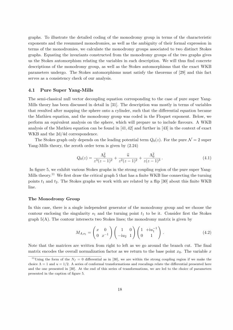
The Stokes graph only depends on the leading potential term Q0(z). For the pure N = 2 super
Yang-Mills theory, the zeroth order term is given by (2.24)
Q0(z) =Λ2
0
z3(z − 1)2+
u
z2(z − 1)2+
Λ20
z(z − 1)3. (4.1)
In figure 5, we exhibit various Stokes graphs in the strong coupling region of the pure super Yang-
Mills theory.11 We first draw the critical graph 5 that has a finite WKB line connecting the turning
points t1 and t2. The Stokes graphs we work with are related by a flip [30] about this finite WKB
line.
The Monodromy Group
In this case, there is a single independent generator of the monodromy group and we choose the
contour enclosing the singularity s1 and the turning point t1 to be it. Consider first the Stokes
graph 5(A). The contour intersects two Stokes lines; the monodromy matrix is given by
MA,s1 =
(x 0
0 x−1
)(1 0
−iu2 1
)(1 +iu−1
1
0 1
). (4.2)
Note that the matrices are written from right to left as we go around the branch cut. The final
matrix encodes the overall normalization factor as we return to the base point x0. The variable x
11Using the form of the Nf = 0 differential as in [30], we are within the strong coupling region if we make the
choice Λ = 1 and u = 1/2. A series of conformal transformations and rescalings relate the differential presented here
and the one presented in [30]. At the end of this series of transformations, we are led to the choice of parameters
presented in the caption of figure 5.
18

critical graph
(A) (B)
Figure 5: The two Stokes graphs of the Nf = 0 case that are related by a simple flip. We also
exhibit the contour used to calculate the monodromy matrix. These graphs were obtained with the
parameters Λ0 = e−iπ4 and u = −1 + i, with the critical graph observed at θ = π.
which appears there is identified with the overall monodromy around the branch cut connecting s1
and t1.
We now turn to the second Stokes graph 5(B). We see that the contour intersects four Stokes
lines, including two lines arising from the flip. The monodromy matrix is given by
MB,s1 =
(x 0
0 x−1
)(1 0
−iu2 1
)(1 −iu−1
2
0 1
)(1 0
+iu1 1
)(1 +iu−1
1
0 1
)
=
(x(u1+u2)
u2ixu1
−i u2xu2xu1
).
(4.3)
We have denoted the variables in Stokes graph 5(B) by variables with tildes since they correspond
to a different Borel resummation. The monodromy matrix MA,s1 must be equivalent to the mon-
odromy matrix calculated on the basis of graph (B), since the monodromy (equivalence class) is a
property of the exact solutions on the Riemann surface Σ.
The Stokes Automorphism
Above, we have the explicit expressions for the monodromy matrices for the two Stokes graphs. The
independent Stokes variables are given by x and u21 in graph 5(A) and the tilde-variables in graph
5(B). Using this notation, we calculate the conjugation invariant traces of the two monodromy
19
matrices:
Tr (MA,s1) = x+1
x+
1
u21x(4.4)
Tr (MB,s1) = x+ u21x+1
u21x. (4.5)
Requiring that the traces of the two monodromy matrices match leads to the map between the
parameters appearing in the two graphs:
u21 = u21
x = x(1 + u21) . (4.6)
This agrees with the Stokes automorphisms derived in [31]. This is also consistent with the general
analysis in [29]. Let us expand on this briefly: the two Stokes graphs lie on either side of the t1− t2flip in the critical graph 5. Since the t1− t2 cycle corresponding to u12 has zero intersection number
with itself, the variable u12 is unaffected by the flip. However, the x variable changes because the
contour around the branch cut has intersection number 1 with the t1 − t2 cycle.
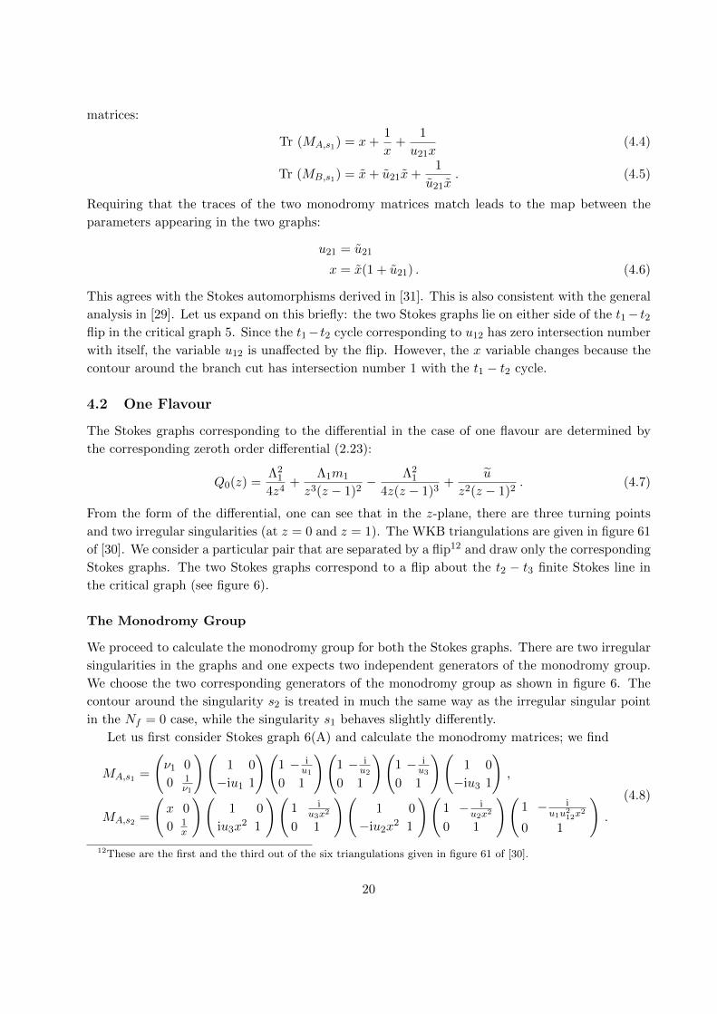
4.2 One Flavour
The Stokes graphs corresponding to the differential in the case of one flavour are determined by
the corresponding zeroth order differential (2.23):
Q0(z) =Λ2
1
4z4+
Λ1m1
z3(z − 1)2− Λ2
1
4z(z − 1)3+
u
z2(z − 1)2. (4.7)
From the form of the differential, one can see that in the z-plane, there are three turning points
and two irregular singularities (at z = 0 and z = 1). The WKB triangulations are given in figure 61
of [30]. We consider a particular pair that are separated by a flip12 and draw only the corresponding
Stokes graphs. The two Stokes graphs correspond to a flip about the t2 − t3 finite Stokes line in
the critical graph (see figure 6).
The Monodromy Group
We proceed to calculate the monodromy group for both the Stokes graphs. There are two irregular
singularities in the graphs and one expects two independent generators of the monodromy group.
We choose the two corresponding generators of the monodromy group as shown in figure 6. The
contour around the singularity s2 is treated in much the same way as the irregular singular point
in the Nf = 0 case, while the singularity s1 behaves slightly differently.
Let us first consider Stokes graph 6(A) and calculate the monodromy matrices; we find
MA,s1 =
(ν1 0
0 1ν1
)(1 0
−iu1 1
)(1 − i
u1
0 1
)(1 − i
u2
0 1
)(1 − i
u3
0 1
)(1 0
−iu3 1
),
MA,s2 =
(x 0
0 1x
)(1 0
iu3x2 1
)(1 i
u3x2
0 1
)(1 0
−iu2x2 1
)(1 − i
u2x2
0 1
)(1 − i
u1u212x2
0 1
).
(4.8)
12These are the first and the third out of the six triangulations given in figure 61 of [30].
20

critical graph
(A) (B)
Figure 6: The critical graph, the pair of Stokes graphs related by a flip and the contours that define
the monodromy group for the Nf = 1 case. The parameters chosen were Λ1 = 2, u = −1/2, and
m1 = 1, and the critical graph was observed at θ = π.
The matrix element on the extreme left in the second monodromy matrix is the naive WKB
monodromy around the branch cut connecting t3 and s2. This contribution x satisfies the relation,
xu12ν1 = 1 . (4.9)
Let us now turn to the Stokes graph 6(B). The monodromy matrices are given by
MB,s1 =
(ν1 0
0 1ν1
)(1 0
−iu1 1
)(1 − i
u1
0 1
)(1 − i
u2
0 1
)(1 0
−iu2 1
)(1 0
−iu3 1
),
MB,s2 =
(x 0
0 1x
)(1 0
iu3x2 1
)(1 −i
u2x2
0 1
)(1 −i
u1u212x2
0 1
).
(4.10)
As before, we define x = 1u12ν1
.
21
The Stokes Automorphism
Now that we have the two sets of monodromy matrices, we calculate the traces of the two sets and
obtain
Tr (MA,s1) = −ν1
(u3
u1+u3
u2
)− 1
ν1
(u1
u2+u1
u3
),
Tr (MA,s2) =1
ν1(u31 + u21) + (u13 + u23)ν1 ,
Tr (MB,s1) = −ν1
(u2
u1+u3
u2+u3
u1
)− 1
ν1
u1
u2,
Tr (MB,s2) =1
ν1(u21) + (u12 + u13 + u23)ν1 .
(4.11)
Substituting u13 = u12u23, and equating the expressions for the traces in powers of ν1 (where we
use the fact that the characteristic exponents are true invariants of the differential equation), we
can extract the Stokes automorphism formulae for the independent contour integrals u21 and u23,
namely:
u23 = u23 , (4.12)
u21 = u21(1 + u32) . (4.13)
Since there is more than one generator of the monodromy group, one can calculate higher-order
invariants by calculating traces of products of the matrices. Using the Stokes automorphism, one
can check that the trace of the products also coincide, thus confirming the identification of the
monodromy group.
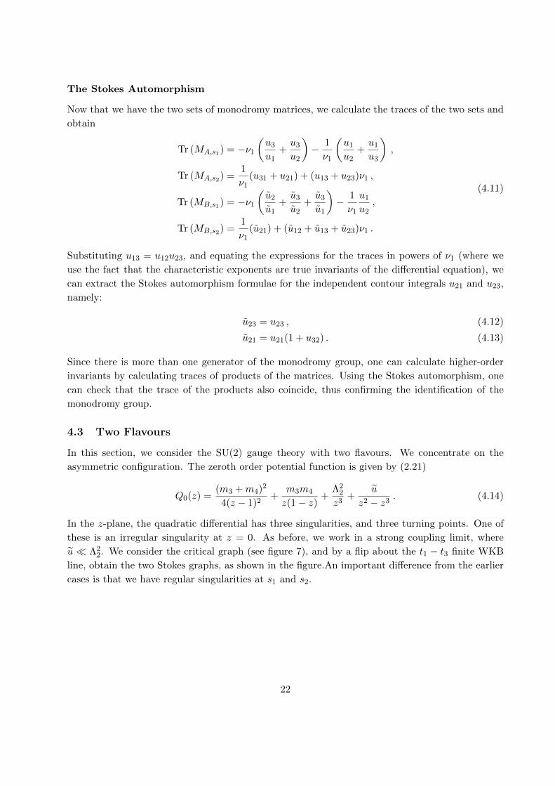
4.3 Two Flavours
In this section, we consider the SU(2) gauge theory with two flavours. We concentrate on the
asymmetric configuration. The zeroth order potential function is given by (2.21)
Q0(z) =(m3 +m4)2
4(z − 1)2+
m3m4
z(1− z)+
Λ22
z3+
u
z2 − z3. (4.14)
In the z-plane, the quadratic differential has three singularities, and three turning points. One of
these is an irregular singularity at z = 0. As before, we work in a strong coupling limit, where
u Λ22. We consider the critical graph (see figure 7), and by a flip about the t1 − t3 finite WKB
line, obtain the two Stokes graphs, as shown in the figure.An important difference from the earlier
cases is that we have regular singularities at s1 and s2.
22

critical graph
(A) (B)
Figure 7: The critical graph and the Stokes graphs for the Nf = 2 case. While plotting the figures,
we used a potential that is conformally equivalent to (4.14). We set Λ2 → i, u→ 12 ,m3 → 0,m4 →
−2. The two Stokes graphs presented were observed at θ = 2π3 and θ = 3π
4 .
The Monodromy Group
In order to calculate the monodromy group, we first consider the Stokes graph 7(A) and determine
the generators
MA,s1 =
(ν1 0
0 1ν1
)(1 − i
u2ν21
0 1
)(1 0
−iu2ν21 1
)(1 0
−iu3ν21 1
)(1 0
−iu1ν21 1
)(1 iu2
0 1
),
MA,s2 =
(ν2 0
0 1ν2
)(1 0
−iu3u232 1
)(1 0
−iu2 1
),
MA,s3 =
(x 0
0 1x
)(1 − i
u2x2
0 1
)(1 0
iu1ν21x
2 1
)(1 − i
u3ν21x2
0 1
).
(4.15)
In the above, x is the naive WKB monodromy around the branch cut connecting t1 and s3. This
contribution satisfies the relation,
u23 ν1 ν2 x = 1 . (4.16)
23

A similar calculation for Stokes graph 7(B), gives us the following monodromy matrices for circling
the singularities
MB,s1 =
(ν1 0
0 1ν1
)(1 − i
u2ν21
0 1
)(1 0
−iu2ν21 1
)(1 0
−iu3ν21 1
)(1 iu2
0 1
),
MB,s2 =
(ν2 0
0 1ν2
)(1 0
−iu1u232 1
)(1 0
−iu3u232 1
)(1 0
−iu2 1
),
MB,s3 =
(x 0
0 1x
)(1 − i
u2x2
0 1
)(1 − i
u3ν21 x2
0 1
)(1 0
iu1ν21 x
2 1
).
(4.17)
Again we have the relation,
u23 ν1 ν2 x = 1 . (4.18)
Stokes Automorphisms
We now compare the traces of the generators of the monodromy group:
TrMA,s1 = TrMB,s1 = ν1 +1
ν1,
TrMA,s2 = TrMB,s2 = ν2 +1
ν2,
TrMA,s3 =1
ν1ν2u32 +
ν1
ν2u21u32 + ν1ν2(u21 +
1
u32) ,
TrMB,s3 =1
ν1ν2u32(u21u32 + 1) +
ν1
ν2u21u32 + ν1ν2
1
u32.
(4.19)
These equations illustrate a recurring feature: the traces of the monodromy matrices around regular
singular points will always be given by the critical exponents, with no uij monodromy factors
entering the expression. This is because the Stokes lines are either all going in or coming out
at such regular singular points. As a result, the relevant Stokes matrices are all either upper
triangular or lower triangular, respectively. This leads to the trivial nature of the trace. The
irregular singularity, on the other hand, has non-trivial structure even at the level of the simple
traces.
Matching the traces between the graphs 7(A) and 7(B) leads to the Stokes automorphism relations,
u31 = u31 ,
u32 = u32(1 + u31) ,
u21 = u21(1 + u31)−1 .
(4.20)
This is once again as expected from the general results of [29] and the intersection numbers between
the various cycles. As a consistency check on the monodromy matrices, we have also computed the
traces of products of matrices, and a similar analysis as above confirms the Stokes automorphisms
(4.20).
24

4.4 Three Flavours
We move on to the SU(2) theory with three flavours. The Seiberg-Witten differential is
Q0(z) =(m3 +m4)2
4(z − 1)2+
m3m4
z(1− z)+m1Λ3
z3+
Λ23
4z4+
u
z2 − z3. (4.21)
There are four turning points and three singularities on the z-plane. The two Stokes graphs in
figure 8 are related by a flip about the t2 − t3 finite line in the critical graph.
critical graph
(A) (B)
Figure 8: The critical graph and the Stokes graphs for the Nf = 3 case. While plotting the figures,
we used a potential that is conformally equivalent to (4.21). We set Λ3 → 1, u→ 2,m1 → −1,m3 →0,m4 → −2. The two Stokes graphs presented were observed at θ = π
2 and θ = 7π12 .
25

The Monodromy Group
For Stokes graph 8(A), we find the generators of the monodromy group:
MA,s1 =
(ν1 0
0 1ν1
)(1 0
iu3ν21 1
)(1 − i
u4ν21ν22
0 1
)(1 − i
u1
0 1
)(1 − i
u2
0 1
)(1 − i
u3
0 1
)(1 0
−iu3 1
),
MA,s2 =
(ν2 0
0 1ν2
)(1 0
−iu4ν22 1
)(1 0
−iu3 1
),
MA,s3 =
(ν3 0
0 1ν3
)(1 0
iu3ν23 1
)(1 iu3ν23
0 1
)(1 0
−iu2ν23 1
)(1 − i
u2ν23
0 1
)(1 − i
u1ν23u212
0 1
)
×
(1 0
−iu1ν23u
212 1
)(1 0
−iu4u243 1
)(1 0
−iu3 1
)(1 − i
u3
0 1
)(1 0
−iu3 1
).
(4.22)
For the Stokes graph 8(B), a similar calculation yields:
MB,s1 =
(ν1 0
0 1ν1
)(1 0
iu3ν21 1
)(1 0
iu2ν21 1
)(1 − i
u4ν21ν22
0 1
)(1 − i
u1
0 1
)(1 − i
u2
0 1
)
×
(1 0
−iu2 1
)(1 0
−iu3 1
),
MB,s2 =
(ν2 0
0 1ν2
)(1 0
−iu4ν22 1
)(1 0
−iu2 1
)(1 0
−iu3 1
),
MB,s3 =
(ν3 0
0 1ν3
)(1 0
iu3ν23 1
)(1 − i
u2ν23
0 1
)(1 − i
u1ν23 u212
0 1
)
×
(1 0
−iu1ν23 u
212 1
)(1 0
−iu4u243 1
)(1 0
−iu3 1
)(1 − i
u3
0 1
)(1 0
−iu3 1
).
(4.23)
The Stokes Automorphism
As in the previous examples, the Stokes automorphism can be obtained by comparing the invariants
built out of the monodromy matrices. The trace of the monodromy around the irregular singular
point s3 is non-trivial and it is important that we express it in terms of independent Stokes variables.
The variables are constrained by the relation
u12u34ν1ν2ν3 = 1 , (4.24)
and similarly for the u variables. We solve for u34 using this relation and choose the independent
variables to be u12 and u23. In terms of these variables, we find that
TrMA,s3 = −ν3u12 − ν1ν2u23(1 + u12)− 1
ν3 u12(1 + u23 + u12u23) . (4.25)
Similarly, from the monodromy around s3 in Stokes graph 8(B) we find
TrMB,s3 = −ν3u12(1
u23+ 1)− ν1ν2(u12 + u23 + u12u23)− u23
ν3u12(1 + u12) . (4.26)
26

Matching the traces leads to the Stokes automorphisms:
u23 = u23 , (4.27)
u12 = u12
(1 +
1
u23
). (4.28)
As a check of our monodromy matrices, we computed the traces of the products of the mon-
odromy matrices. These imply the same Stokes automorphism as above.
4.5 The Conformal Theory
We consider Stokes graphs in a strong coupling region of the conformal SU(2) theory. The zeroth
order potential has four regular singular points and four turning points.
In particular, we consider the Stokes graphs corresponding to two out of the six triangulations
in figure 74 of [30] (see figure 9(A) and (C)).13 It can be seen that the two Stokes graphs are related
by a double flip, a simultaneous flip about the t1 − t3 and t2 − t4 finite WKB lines in the critical
graph. We realize the double flip as two alternative sequences of two single flips. We provide
the corresponding intermediate graphs after the single flips and perform the calculation we have
familiarized ourselves with by now.
Let us first consider the flip from Stokes graph 9(A) to 9(B′) via the t1 − t3 flip. The relevant
Stokes graphs and contours that generate the monodromy group are given in figure 10.
The Monodromy Group
For Stokes graph 9(A), using the contours as shown in figure 10(A), the monodromy matrices are
given by
MA,s1 =
(ν1 0
0 1ν1
)(1 0
iu4ν21 1
)(1 −iu1u213ν
21
0 1
)(1 − i
u4
0 1
)(1 0
−iu4 1
),
MA,s2 =
(ν2 0
0 1ν2
)(1 0
iu4ν22 1
)(1 iu4ν22
0 1
)(1 0
−iu1u213ν
21ν
22 1
)(1 0
−iu3u213ν
21ν
22 1
)
×
(1 0
−iu2u224 1
)(1 0
−iu4 1
)(1 − i
u4
0 1
)(1 0
−iu4 1
),
MA,s3 =
(ν3 0
0 1ν3
)(1 0
iu4ν23 1
)(1 0
iu1u213ν
23 1
)(1 0
iu3ν23 1
)(1 −iu2ν23ν
24
0 1
)
×
(1 − i
u3
0 1
)(1 0
−iu3 1
)(1 0
−iu1u213 1
)(1 0
−iu4 1
),
MA,s4 =
(ν4 0
0 1ν4
)(1 0
−iu2ν24 1
)(1 0
−iu3 1
)(1 0
−iu1u213 1
)(1 0
−iu4 1
).
(4.29)
13Our graphs are topologically equivalent to those appearing in [30].
27

(A)
(B)
(B')
(C)
critical graph
Figure 9: The critical graph and a pair of Stokes graphs for the conformal SU(2) theory. A double
flip relates one graph to the other. We refer the reader to B.1 for details.
28

(A) (B')
Figure 10: The two Stokes graphs related by the t1 − t3 flip.
Next we consider the Stokes graph 9(B′) and move along the contours Ck around the singularities
as shown in figure 10(B′). We compute the monodromy matrices:
MB′,s1 =
(ν1 0
0 1ν1
)(1 0
iu4ν21 1
)(1 −iu3ν21
0 1
)(1 −iu1u213ν
21
0 1
)(1 − i
u4
0 1
)(1 0
−iu4 1
),
MB′,s2 =
(ν2 0
0 1ν2
)(1 0
iu4ν22 1
)(1 iu4ν22
0 1
)(1 0
−iu1u213ν
21ν
22 1
)
×
(1 0
−iu2u224 1
)(1 0
−iu4 1
)(1 − i
u4
0 1
)(1 0
−iu4 1
),
MB′,s3 =
(ν3 0
0 1ν3
)(1 0
iu4ν23 1
)(1 0
iu3ν23 1
)(1 −iu2ν23ν
24
0 1
)
×
(1 −iu1
0 1
)(1 − i
u3
0 1
)(1 0
−iu3 1
)(1 0
−iu4 1
),
MB′,s4 =
(ν4 0
0 1ν4
)(1 0
−iu2ν24 1
)(1 0
−iu3 1
)(1 0
−iu4 1
).
(4.30)
We now implement the t2− t4 flip to go from Stokes graph 9(B′) to graph 9(C). The relevant Stokes
graphs and contours are given in figure 11. Notice that the base point of the contours in figure 11
is different from that used in figure 10, however, this is irrelevant because the monodromy group is
independent of the choice of a base point. The monodromy matrices for the (B′) graph are given
29

(C)(B')
Figure 11: The t2 − t4 flip and the contours around the singularities.
by
MB′,s1 =
(ν1 0
0 1ν1
)(1 −iu3ν21
0 1
)(1 −iu1u213ν
21
0 1
)(1 − i
u4
0 1
),
MB′,s2 =
(ν2 0
0 1ν2
)(1 iu4ν22
0 1
)(1 0
−iu1u213ν
21ν
22 1
)(1 0
−iu2u224 1
)(1 0
−iu4 1
)(1 −iu4
0 1
),
MB′,s3 =
(ν3 0
0 1ν3
)(1 0
iu3ν23 1
)(1 −iu2ν23ν
24
0 1
)(1 −iu1
0 1
)(1 −iu3
0 1
)(1 0
−iu3 1
),
MB′,s4 =
(ν4 0
0 1ν4
)(1 0
−iu4ν24 1
)(1 0
−iu2ν24 1
)(1 0
−iu3 1
).
(4.31)
Finally, we consider Stokes graph 9(C) and calculate the generators of the monodromy group
MC,s1 =
(ν1 0
0 1ν1
)(1 −iu3ν21
0 1
)(1 −iu1u213ν
21
0 1
)(1 −iu2u224
0 1
)(1 − i
u4
0 1
),
MC,s2 =
(ν2 0
0 1ν2
)(1 iu4ν22
0 1
)(1 iu2u224ν
22
0 1
)(1 0
−iu1u213ν
21ν
22 1
)(1 0
−iu2u224 1
)
×
(1 −iu2u224
0 1
)(1 −iu4
0 1
),
MC,s3 =
(ν3 0
0 1ν3
)(1 0
iu3ν23 1
)(1 −iu4ν23ν
24
0 1
)(1 −iu2ν23ν
24
0 1
)(1 −iu1
0 1
)(1 −iu3
0 1
)(1 0
−iu3 1
),
MC,s4 =
(ν4 0
0 1ν4
)(1 0
−iu4ν24 1
)(1 0
−iu3 1
).
(4.32)
30

The Stokes Automorphism for the Double Flip
The monodromy matrices obtained above by encircling the singularities in both the pairs of graphs
in the sequence of flips have standard traces, since all the singularities are regular. Hence, in order
to compute the transformation of Voros symbols, we compute the traces of products of monodromy
matrices. We express the traces in terms of the variables u13 and u34 in the t1 − t3 flip and in
terms of the variables u42 and u21 in the t2 − t4 flip. Since the entries of the matrices are a bit
cumbersome, we merely present the results; here the variables in a given Stokes graph are denoted
with the appropriate superscript: This gives us the Stokes automorphism relations.
uA13 = uB′
13 , uA34 = uB′
34 (1 + uB′
13 ) (4.33)
uB′
42 = uC42, uB′
21 = uC21(1 + uC42) (4.34)
Upon composing the Stokes relations from the two single flips, we obtain the desired Stokes relation
for the double flip from Stokes graph (A) to (C). If we consider a counter-clockwise loop encircling
both the branch cuts and the four singularities in graphs (A), (B′) and (C), we get the relation,
u13u42ν1ν2ν3ν4 = 1 (4.35)
There is an analogous condition that is given by
u43u12ν1ν2ν3ν4 = 1 . (4.36)
Using these and the Stokes automorphisms for the sequence of flips, we obtain the following relations
for the independent variables of the Stokes graphs (A) and (C):
uA13 = uC13
uA34 = uC34
1 + uC13
1 + uC42
. (4.37)
Because the double flip is composed of single flips, each taking place within their own arena, the
final result for the double flip is a composition of the result for single flips [29].
So far, we have implemented the double flip via a sequence of two single flips, (A)→ (B′)→(C) as in figure 9. The double flip can equivalently be implemented by a different sequence of two
single flips, (A)→ (B)→ (C) as shown in figure 9. We have checked that this results in the same
Stokes automorphism relations as were arrived at earlier. This is further confirmation of the rules
for computing the monodromy groups and of our resolution of the double flip into two single flips.
Pops
Finally, we consider two Stokes graphs that are related by a pop rather than a flip, in the conformal
gauge theory. We concentrate on the situation depicted in figure 12 (see appendix B for more
details). This corresponds to the degenerate triangulations in figure 74 of [30]. The pop is expected
to give rise to a trivial Stokes automorphism for our closed loop Voros symbols. We first consider
31

(A) (B)
Figure 12: The two Stokes graphs related by a pop. We refer the reader to B.2 for details.
graph 12(A) and calculate the generators of the monodromy group. As the closed contour goes
around s1 counter-clockwise,
MA,s1 =
(ν1 0
0 1ν1
)(1 − i
u4ν21
0 1
)(1
iν22u2u221
0 1
)(1 −iu10 1
)(0 i
i 0
)(1 0
− iν22u1
1
)(0 −i−i 0
)︸ ︷︷ ︸
(1 − i
u2
0 1
). (4.38)
Next we compute the monodromy matrix as we traverse a closed contour that goes around the
singularity s2
MA,s2 =
(ν2 0
0 1ν2
)(1 iu2ν22
0 1
)(0 i
i 0
)(1 0iu1
1
)(0 −i−i 0
)︸ ︷︷ ︸
(0 i
i 0
)(1 iu1
0 1
)(0 −i−i 0
)
×
(0 i
i 0
)(1 0−iν22u1
1
)(0 −i−i 0
)︸ ︷︷ ︸
(1 − i
u2
0 1
).
(4.39)
32
Around the singularity s3 and s4, we find
MA,s3 =
(ν3 0
0 1ν3
)(1 0
−iu2ν23 1
)(1 0
iu4u234ν24
1
)(1 0
−iu3 1
)
×
(0 i
i 0
)(1 −iu3
ν24
0 1
)(0 −i−i 0
)︸ ︷︷ ︸
(1 0
−iu4 1
),
MA,s4 =
(ν4 0
0 1ν4
)(1 0
iu4ν24 1
)(0 i
i 0
)(1 iu3
0 1
)(0 −i−i 0
)︸ ︷︷ ︸
(0 i
i 0
)(1 0iu3
1
)(0 −i−i 0
)
×
(0 i
i 0
)(1 −iu3
ν24
0 1
)(0 −i−i 0
)︸ ︷︷ ︸
(1 0
−iu4 1
).
(4.40)
In the above, the set of matrices clubbed together by an underbrace gives the rule for crossing a
Stokes line that runs through a branch cut into the other sheet and approaches the turning point.
We repeat the above exercise for Stokes graph 12(B) and the monodromy matrices around the
singularities in this case are given by
MBs1=
(ν1 0
0 1ν1
)(1 −iu4ν21
0 1
)(1
iν22u2u221
0 1
)(1−iν22u1
0 1
)(1 −iu10 1
)(1 −iu20 1
),
MBs2=
(ν2 0
0 1ν2
)(1 iu2ν22
0 1
)(0 i
i 0
)(1 −iu1ν
22
0 1
)(1 0iu1
1
)(1 0
iu1 1
)(0 −i−i 0
)(1 −iu20 1
),
MBs3=
(ν3 0
0 1ν3
)(1 0
−iu2ν23 1
)(1 0
iu4u234ν24
1
)(1 0−iu3ν24
1
)(1 0
−iu3 1
)(1 0
−iu4 1
),
MBs4=
(ν4 0
0 1ν4
)(1 0
iu4ν24 1
)(0 −i−i 0
)(1 0−iu3ν24
1
)(1 iu3
0 1
)(1 0iu3
1
)(0 i
i 0
)(1 0
−iu4 1
).
(4.41)
Again, it can be checked that the monodromy matrices have standard traces in both the graphs.
Similarly it can be checked that the product of matrices from both the graphs have the same
traces. Thus, we have a consistency check on our calculation, which is the triviality of the Stokes
automorphism acting on the Voros symbols of graphs related by a pop (3.34).
5 The Gauge Theory Perspective
We have computed the monodromy groups associated to the differential equations governing the
instanton partition function with surface operator insertion in terms of the exponents νi charac-
terizing the singularities, and the Borel resummed monodromies uij . The characteristic exponents
are readily calculated in terms of the masses of the gauge theory using the explicit expression of
the differential equation. In this section, we further relate the exact WKB parameters uij with the
Seiberg-Witten periods a and aD, which are leading order approximations. As a result, we obtain
the monodromy groups in terms of the (deformed, resummed) gauge theory data. Next, we present
ideas on how to exploit this information to obtain non-perturbative corrections to the prepotential.
33

5.1 The Seiberg-Witten Variables
We start by relating the monodromies uij to more standard Seiberg-Witten data. In the following
figures, we mark only the turning points and the singularities on the Riemann surface, and identify
the α and β cycles of the genus one Seiberg-Witten curve. For the conformal case [35], the cycles
are identified as in figure 13. The cycles have a smooth limit when the masses are set to zero, i.e.
when the turning points coincide with the singularities. Further, in [35], it was explicitly checked
that the prepotential of the conformal theory, obtained by calculating the period integrals with this
choice of cycles, matches the results from equivariant localization methods. Once this identification
is made, it is possible to go down in the number of flavors sequentially, each time identifying the α
and β cycles, until we finally reach the Nf = 0 theory, where we obtain agreement with the results
of [31].
The Conformal Theory
From figure 13, we read off the identification
u13ν1ν3 = ea, u34ν3ν4 = eaD . (5.1)
Figure 13: Nf = 4 cycles
The Stokes automorphisms we have derived for the conformal theory then imply the following
relations for the gauge theory variables between the Stokes graphs 9(A) and 9(C):
(ea)A = (ea)C ,
(eaD)A = (eaD)C
[ 1 + ν−11 ν−1
3 (ea)C
1 + ν−12 ν−1
4 (e−a)C
]. (5.2)
We will comment on the meaning of these relations after we list the cycles and appropriate gauge
theory variables for the asymptotically free cases.
Three Flavours
From figure 14, for the three flavours case, we find the relation
u12ν1ν2 = ea, u23ν2ν3 = eaD . (5.3)
34

Figure 14: Nf = 3 cycles
As before we can write the Stokes automorphisms in terms of the gauge theory variables but we
suppress these details and only give the choice of cycles in our subsequent examples.
Two Flavours
For two flavours, from figure 15 we have,
u23ν1ν2 = ea, u31ν1 = eaD . (5.4)
Figure 15: Nf = 2 cycles
One Flavour
When we are left with a single flavour, we find from figure 16
u12ν1 = ea, u23 = eaD . (5.5)
Pure Super Yang-Mills
Finally, for pure super Yang-Mills, we have from figure 17
u21 = eaD , x = ea . (5.6)
35

Figure 16: Nf = 1 cycles
Figure 17: Nf = 0 cycles
The Stokes automorphisms derived in Section 4.1 can then be reinterpreted in terms of the gauge
theory variables as a relation between a and aD,
eaD = eaD ,
ea = ea(1 + eaD) . (5.7)
One can check that these precisely coincide with the Stokes automorphisms obtained for the pure
super Yang-Mills case in [31].
5.2 The Non-Perturbative Prepotential
In this subsection, we restrict ourselves to some preliminary remarks on how to exploit the results
we have obtained on the monodromy group to find non-perturbative corrections to the prepotential
(parameterized in terms of the given exact WKB monodromy data). We note that the expressions
ea(ε1) and eaD(ε1) used above (where we have now rendered explicit the ε1 dependence) refer to
the exact WKB, Borel resummed ε1 perturbation series. At leading order in ε1, the first term
in the expansion matches the Seiberg-Witten periods a(0) and aD(0). In the ε1-deformed theory,
these are corrected as a perturbation series in ε1. In the exact WKB approach, these perturbation
series are Borel resummed, but the result depends on the region of Borel resummation, and the
resummed expressions ea(ε1) depend on the phase of Borel resummation, or equivalently, on the
phase of ε1. Thus, the above identifications undergo the Stokes automorphisms of which we have
discussed many an example. Note that when we refer to such expressions, we have in mind that
they are valid with a given resummation angle.
36

The monodromy group itself, and in particular the gauge invariant traces of products of mon-
odromy matrices, are exact invariants of the solution to the differential equations. In [31], it was
proposed in the context of the theory with zero flavours to solve the equation for the Borel re-
summed period a(ε1) in terms of the invariant quantity aexact, determined by the exact periodicity
(or Floquet exponent, or monodromy) of the exact solution to the (Mathieu) differential equation.
This solution is valid at a particular resummation angle, and a is identified with aexact, up to non-
perturbative corrections. Near a point in moduli space where a perturbative expansion is possible,
like the weak, magnetic or dyonic point, we can then solve the relation in terms of a transseries [28].
On the other hand, since in this case aD(ε1) is independent of the Borel resummation angle, we can
posit aexactD = aD(ε1) (independently of the specification of the resummation angle). The variable
u determining the derivative of the prepotential is known as a function of a, and therefore as a
function of aexact. Inverting this relation and calculating the dual period integrals allows one to
calculate non-perturbative corrections to the prepotential F .
Thus, one application of the identifications above is to attempt to integrate up the non-
perturbative relation between the period a and the parameters coding the exact monodromy group,
towards non-perturbative corrections to the prepotential F . The encompassing case in which to
execute this program is the conformal Nf = 4 theory.
6 Conclusions
In our work, we filled in many details of the connection between conformal field theory and four-
dimensional gauge theory which was made handily available starting from the matching of partition
functions and correlators in [9]. We applied the technology developed in [11–13, 32] to study in
greater detail SU(2) super Yang-Mills theories with a varying number of flavours. We thus provided
a complete list of εi-deformed differential equations satisfied by the five-point conformal block with
surface operator insertion, in the irregular conformal block limit. Subsequently, we took a semi-
classical limit and analyzed the resulting differential equations with exact WKB methods. We used
this technology to give a detailed parameterization of the monodromy groups in terms of Voros
symbols and external conformal dimensions or, in the language of gauge theory, in terms of Borel
resummed ε1-deformed Seiberg-Witten periods and masses. The Borel resummed variables depend
intrinsically on the resummation angle (and the phase of ε1), and we illustrated how to bridge this
ambiguity using Stokes automorphisms, with at least one illustration for each number of flavours.
The Stokes automorphisms we obtained are consistent with the general theorems proved in [29].
The one subtlety arose in the case of the conformal gauge theory: in this case, we analyzed a pair of
Stokes graphs that were related by a simultaneous flip along two independent finite WKB lines. In
such a case, we showed that the resulting Stokes automorphisms could be obtained by treating the
double-flip as a sequence of single flips. We demonstrated consistency of this approach by checking
that the final Stokes automorphisms between the Stokes graphs were independent of the order in
which the single flips were taken.
We believe it is instructive to develop these most elementary of N = 2 models in still further
detail. There are many avenues to explore. As was mentioned in the previous section, it should be
possible to calculate non-perturbative corrections in ε1 to the prepotential, by suitably generalizing
37

the analysis that was done for the case of pure super Yang-Mills [31]. Similarly, it should be
informative to match the cluster algebra description of Stokes automorphisms of [29] to the cluster
algebra description of the spectrum of BPS states [36]. (See also e.g. [29, 37,38].)
In the present work, we studied general properties of the Borel resummed wave-functions of the
null vector decoupling equations in the semi-classical limit, without focusing on the specific form
of the wave-function. An interesting direction would be to study in greater detail the dependence
of the five-point conformal block on the insertion point of the degenerate operator. This should
yield non-trivial information about the gauge theory in the presence of a surface operator. Most
interestingly, perturbative and non-perturbative corrections in ε2 can now be studied from the
differential equation point of view.
All these projects have straightforward extensions, both to the N = 2? theory, where the
Riemann surface is of genus one [7], as well as to higher rank conformal gauge theories, the simplest
of which is super Yang-Mills theory with SU(N) gauge group and 2N fundamental flavours. As
explained in Section 5, one not only needs the description of the monodromy group, but also
requires a local expansion of the period integrals in terms of the Coulomb moduli in order to carry
out the goal of calculating corrections to the prepotential that are non-perturbative in ε1. For the
N = 2? theory with gauge group SU(2), the null vector decoupling equation for the toroidal block
has been well studied in the semi-classical limit (see e.g. [16,45,46]) and the instanton series for the
prepotential has been resummed in terms of modular functions [47]. One can therefore attempt
to study the monodromy group along the lines of the present paper and hope to carry out the
proposal put forward in Section 5. For higher rank N = 2? theories, there has been much progress
on the gauge theory side in resumming the instanton expansion for the prepotential using modular
anomaly equations in deformed gauge theories with arbitrary gauge group [48, 49]. It remains an
open problem to reproduce these successes using conformal field theory methods and to do the
corresponding WKB analysis.
For the higher rank (and undeformed) SQCD theories, the instanton series has been resummed
in a special locus with ZN symmetry [52,53]. From the CFT approach to the problem, one has to
work with Toda theory [50] and the corresponding null vector decoupling equations in Toda have
been analyzed recently in [51]. In the semi-classical limit, such differential equations can also be
derived using a saddle point analysis of the Nekrasov integrand [34] and the resulting deformed
Seiberg-Witten curve. It would be interesting to analyze these higher order differential equations
using exact WKB methods and make contact with the general approach to these systems using
spectral networks [54,55].
Acknowledgments
We would like to thank Anirban Basu, Soumyadeep Bhattacharya, Eleonora Dell’Aquila, Anshuman
Maharana, Gautam Mandal, Shiraz Minwalla, and Ashoke Sen for useful discussions. We would
especially like to thank Eleonora Dell’Aquila for help with the pictures. S.A. and D.P.J. would
like to thank TIFR, Mumbai for hospitality. D.P.J. would also like to thank IMSc, Chennai for
hospitality during the course of this work. D.P.J. was partially supported by DAE XII-plan grant
38

12-R& D-HRI-5.02-0303. J.T. would like to acknowledge support from the grant ANR-13-BS05-
0001.
A The Null Vector Decoupling with Irregular Blocks
In this section, we derive in detail the null vector decoupling equations that involve irregular
conformal blocks. These equations were summarized in a different form in [11]. Our final results
are listed in section 2.
A.1 One Irregular Puncture
The case of Nf = 4 is standard and is described in section 2 in sufficient detail. We turn to the
conformal block involving an irregular puncture. This involves rendering one flavour very massive.
A.1.1 Nf = 3
From the gauge theory point of view, the flavour decoupling is carried out by taking the limit:
m2 →∞ q → 0 with Λ3 = q m2 finite . (A.1)
The parameter Λ3 has mass-dimension one and is the strong coupling scale of the SU(2) gauge
theory with Nf = 3. As shown in [13], in the conformal field theory this involves a collision of the
regular conformal block at z = q and z = 0 and leads to an irregular conformal block at z = 0. We
now consider the five point conformal block with the insertion of the degenerate field Φ2,1(z):
〈Vα4(∞)Vα3(1)I(4)(0) Φ2,1(z)〉 . (A.2)
The Ward identity for this chiral conformal block can be obtained by considering the five point
block relevant for the conformal Nf = 4 and scaling the wave-function in the following way [11,13]:
Ψ(z, q) = q−2α1α2 ψ3(z,Λ3) . (A.3)
On the rescaled wave-function ψ3(z), the q-derivative is traded for a Λ3-derivative. Combining
these, and taking the decoupling limit, we obtain the null vector decoupling equation for the
Nf = 3 theory:[− ε21
∂2
∂z2+
(m3 +m4)2
4(z − 1)2+
m3m4
z(1− z)+m1Λ3
z3+
Λ23
4z4− ε21
4(z − 1)2+ ε22
(3− 4z)
4z(z − 1)2
+1
z2 − z3
(− ε1ε2Λ3
∂
∂Λ3+m2
1 +m1(ε1 + ε2))
+ ε1ε2
(1− 2z
z − z2
∂
∂z+
1− 2z
2z(z − 1)2
)]ψ3(z,Λ3) = 0 .
(A.4)
The quartic pole at z = 0 in the OPE between the stress tensor and the irregular block explains
our notation: we denote such an irregular block by I(4)(0).
39

A.1.2 Nf = 2: asymmetric realization
One can take a further limit in which we decouple the mass m1:
m1 →∞ Λ3 → 0 with Λ22 = m1Λ3 finite . (A.5)
Simultaneously, we rescale the wave-function by
ψ3(z,Λ3) = Λ1
ε1ε2(m2
1+m1(ε1+ε2))
3 ψ2(z,Λ2) . (A.6)
From the conformal field theory perspective, this amounts to tuning the coefficient of the quartic
pole to zero, leaving behind only a cubic pole. This corresponds to the four point conformal block
〈Vα4(∞)Vα3(1)I(3)(0) Φ2,1(z)〉 . (A.7)
The null vector decoupling equation takes the form:[−ε21
∂2
∂z2+
(m3 +m4)2
4(z − 1)2+
m3m4
z(1− z)+
Λ22
z3− ε1ε2
2(z2 − z3)Λ2
∂
∂Λ2
+ε1ε2
(1− 2z
z − z2
∂
∂z+
1− 2z
2z(z − 1)2
)− ε21
4(z − 1)2+ ε22
(3− 4z)
4z(z − 1)2
]ψ2(z,Λ2) = 0 . (A.8)
The equation exhibits a cubic pole at the irregular singularity z = 0.
A.2 Two Irregular Punctures
Let us begin with the five point conformal block in which we have regular conformal primaries at
zi, with i ∈ 1, 2, 3, 4 and the degenerate field at z. In equation (2.5), we have obtained the null
vector decoupling equation for this case. We now set z1 = 0, z2 = q and z4 = 1 and consider the
simultaneous collision of punctures such that q → 0 and z3 → 1. We rescale the wave-function as
in [13]
Ψ(zi) = q−2α1α2(z3 − 1)−2α3α4ψ(z,Λ, Λ) . (A.9)
In order to get finite results, we take the limit
m2 →∞ , q → 0 with Λ = q m2 finite ,
m3 →∞ , (z3 − 1)→ 0 with Λ = (z3 − 1)m3 finite . (A.10)
Note that this introduces two independent scales in the problem. The conformal block we are
considering is a three point function, with two irregular punctures of quartic order and a degenerate
field Φ2,1(z):
〈I(4)(1)I(4)(0) Φ2,1(z)〉 . (A.11)
The parameters Λ and Λ respectively represent the quartic pole coefficient at z = 0 and z = 1.
After the wave-function rescaling and the decoupling limits, we obtain the null vector decoupling
equation for such a conformal block with two such irregular singularities and the degenerate field:
40
[− ε21
∂2
∂z2+
Λ2
4z4+
Λm1
z3(z − 1)2+
Λm4
z(z − 1)3+
Λ2
4(z − 1)4+ ε1ε2
3z − 1
z(z − 1)
∂
∂z+
(2ε1ε2 + 3ε22)(2− 3z)
4z(z − 1)2
+1
z2(z − 1)2
(− ε1ε2Λ
∂
∂Λ− 2Λm1 +m2
1 +m1(ε1 + ε2))]ψ2(z,Λ, Λ) = 0 .
(A.12)
We can tune the two scales suitably in order to obtain the null vector decoupling equations for the
remaining gauge theories of our focus.
A.2.1 Nf = 2: symmetric realization
We set Λ = −Λ = Λ2, in which case we obtain the null vector decoupling equation:[− ε21
∂2
∂z2+
Λ22
4z4+
Λ2m1
z3(z − 1)2− Λ2m4
z(z − 1)3+
Λ22
4(z − 1)4+ ε1ε2
3z − 1
z(z − 1)
∂
∂z+
(2ε1ε2 + 3ε22)(2− 3z)
4z(z − 1)2
+1
z2(z − 1)2
(− ε1ε2Λ2
∂
∂Λ2− 2Λ2m1 +m2
1 +m1(ε1 + ε2))]ψ2(z,Λ2) = 0 .
(A.13)
A.2.2 Nf = 1
We set Λ = Λ1 and Λ → 0 such that Λm4 = −Λ21
4 is a finite combination. In other words, the
relevant conformal block of interest is
〈I(3)(1)I(4)(0) Φ2,1(z)〉 . (A.14)
The coefficient of the cubic pole at z = 1 is tuned and related to that of the quartic pole at z = 0.
Such a conformal block satisfies the null vector decoupling equation:[− ε21
∂2
∂z2+
Λ21
4z4+
Λ1m1
z3(z − 1)2− Λ2
1
4z(z − 1)3+ ε1ε2
3z − 1
z(z − 1)
∂
∂z+
2− 3z
4z(z − 1)2(2ε1ε2 + 3ε22)
+1
z2(z − 1)2
(− ε1ε2Λ1
∂
∂Λ1− 2Λ1m1 +m2
1 +m1(ε1 + ε2))]ψ1(z,Λ1) = 0 . (A.15)
A.2.3 Nf = 0
As for the earlier case with Nf = 2 in the asymmetric realization, in order to obtain finite results,
one has to rescale the wave-function
ψ(z,Λ, Λ) = Λ1
ε1ε2(m2
1+m1(ε1+ε2))ψ0(z,Λ0) . (A.16)
We set Λ → 0 and Λ → 0 such that the combinations m1Λ = Λ20 and m4Λ = Λ2
0 are equal and
finite. The relevant conformal block is given by
〈I(3)(1)I(3)(0) Φ2,1(z)〉 . (A.17)
41

This satisfies the null vector decoupling equation:[− ε21
∂2
∂z2+
Λ20
z3(z − 1)2+
Λ20
z(z − 1)3+ ε1ε2
3z − 1
z(z − 1)
∂
∂z+
2− 3z
4z(z − 1)2(2ε1ε2 + 3ε22)
+1
z2(z − 1)2
(− 1
2ε1ε2Λ0
∂
∂Λ0− 2Λ2
0
)]ψ0(z,Λ0) = 0 . (A.18)
B Stokes Graphs
In this section, we plot actual machine-generated Stokes graphs for the Nf = 4 theory as represen-
tative examples. The Stokes lines are defined by the condition
Im
[∫ x
x0
dx′√Q0(x′)
]= 0 . (B.1)
The red dots indicate singularities, and the blue dots indicate turning points. It is important to
remember that what is relevant for the monodromy calculations is the topology of the Stokes graph.
The cartoons in the body of the paper abstract away from graphs given in this appendix.
B.1 The Double Flip
The potential we use to plot these Stokes graphs has a convenient Z4 symmetric form [30]
Q0(z) =z4 − u
(z4 − 1
)(z4 − 1)4 , (B.2)
where the singularities are at z1 = 1, z2 = i, z3 = −1, and z4 = −i. This potential is arrived at via
an SL(2,C) transformation of (2.18) that maps all singularities to finite points for ease of plotting.
The masses of the fundamental hypermultiplets are ma = 14za. We have made the choice u = 1
2 for
plotting the double flip Stokes graphs in figure 18.
B.2 The Pop
We continue to work with the potential (B.2) and, in order visualize the pops in figure 19, we have
made the choice u = 12exp
(310 iπ
).
C The Saddle Point Analysis
We discussed regular (irregular) conformal blocks associated to two-dimensional conformal field
theories that, via the 2d/4d correspondence, are dual to four-dimensional Ω-deformed conformal
(respectively, asymptotically free) gauge theories. The null vector decoupling equations together
with the conformal Ward identities allow us to arrive at Schrodinger equations that govern an
integrable system related to the Ω-deformed gauge theory. While these analyses are exact in ε2, it
is enlightening to see how the ε2 → 0 limit of these differential equations are derived from purely
42

-1.5 -1.0 -0.5 0.5 1.0 1.5
-2
-1
1
2
(a) Before the double flip
-2 -1 1 2
-1.5
-1.0
-0.5
0.5
1.0
1.5
(b) After the double flip.
-1.5 -1.0 -0.5 0.5 1.0 1.5
-1.5
-1.0
-0.5
0.5
1.0
1.5
(c) The critical graph.
Figure 18: Sequence of Stokes graphs related by a double flip about the critical graph
43

-3 -2 -1 1 2 3
-2
-1
1
2
(a) Before the pop.
-3 -2 -1 1 2 3
-2
-1
1
2
(b) After the pop.
-3 -2 -1 1 2 3
-2
-1
1
2
(c) The critical graph.
Figure 19: Sequence of Stokes graphs related by a pop about the critical graph
44

gauge-theoretic considerations. This will serve as a consistency check of the 2d/4d correspondence,
and our calculations.
In this section, we explain how to derive differential equations starting from saddle-point dif-
ference equations, valid for any SU(N) theory with Nf = 2N fundamental hypermultiplets. We
specialize to the case of the conformal SU(2) theory (Nf = 4) and consider various decoupling
limits that give asymptotically free theories with fewer fundamental hypermultiplets.
Our analysis begins with the Nekrasov partition function, and considers its saddle-points in
the limit ε2 → 0, with ε1 held constant and finite [34, 39, 40, 44]. The result of this analysis is the
ε1-deformed Seiberg-Witten equation:
y (x) + qM (x− ε1)
y (x− ε1)= (1 + q)P (x) . (C.1)
Here, q is the instanton counting parameter. The gauge polynomial P (x) is of degree N and encodes
the Coulomb moduli of the gauge theory. The flavour polynomial M(x) is of degree 2N , and we
choose to factorize it into two pieces:
M(x) = A(x)D(x) , (C.2)
where A(x) and D(x) are degree N polynomials. As should be evident, this decomposition is far
from being unique. Different decompositions can be mapped to the different ways in which the
flavour symmetry is realized in the type II construction using two NS5 branes and a stack of D4
branes. One can associate the number of semi-infinite D4 branes on each side of the NS5 branes
with the degree of the polynomials A(x) and D(x). We now peel off a factor of A(x) from the
function y(x) and express the remainder as the ratio of some rational function Q(x) as
y(x) = A(x)Q(x)
Q(x− ε1). (C.3)
There are other ways to perform the split but this one will reduce, in the ε1 → 0 limit, to the
correct M-theory curve. The result of these decompositions gives us the Baxter TQ-relation
A(x)Q(x) + qD(x− ε1)Q(x− 2ε1)− (1 + q)P (x)Q(x− ε1) = 0. (C.4)
We now trade Q(x) for its Fourier transform [34]
Ψ(t) =∑x∈Γ
Q(x) e−x/ε1 , (C.5)
and arrive at the differential equation of order N :[A(x) + qD(x− ε1) t−2 − (1 + q)P (x) t−1
]Ψ(t) = 0, (C.6)
where in the above equation, the Fourier transform effectively sends x 7→ −ε1t∂t.
45
C.1 Nf = 4
We specialize to the case of the conformal SU(2) gauge theory, with Nf = 4. The matter polyno-
mials we start with are
D(x) =(x−m1 +
ε12
)(x−m2 +
ε12
), (C.7)
A(x) =(x−m3 +
ε12
)(x−m4 +
ε12
). (C.8)
The gauge polynomial is
P (x) = x2 − q(m1 +m2 +m3 +m4
1 + q
)x− uS
1 + q. (C.9)
Substituting this into the difference equation and taking the Fourier transform as described
earlier leads to a second order differential equation. We would like this differential equation to be
of the Schrodinger form, i.e. with no linear derivative terms. This may be achieved by peeling off
an appropriate factor.14 The resulting differential equation is[−ε21
∂2
∂t2+Q(t, ε1)
]Ψ(t) = 0, (C.10)
where the potential term Q(t, ε1) has an expansion in powers of ε1. In addition, we further shift of
the Coulomb modulus uS ,
uS = −u+q − 1
2
(m2
1 +m22
)+ q
[m1m2 +m3m4 +
1
2(m1 +m2) (m3 +m4)
]+ε214
(1 + q) (C.11)
Denoting the order εm1 coefficient in the potential by Qm(t), we obtain the non-zero potential terms:
Q0(t) = − u
t(t− 1)(t− q)+
(m1 −m2)2
4t2+
(m1 +m2)2
4(t− q)2+
(m3 +m4)2
4(t− 1)2+m2
1 +m22 + 2m3m4
2t(1− t),
(C.12)
Q2(t) = − 1
4t2− 1
4(t− 1)2− 1
4(t− q)2+
1
2(t− 1)(t− q). (C.13)
This matches the potentials in the text obtained from the null vector decoupling equations (2.18).
C.2 Nf = 3
The Nf = 3 case is obtained by decoupling one of the masses; we choose here to send m2 → ∞,
while simultaneously sending q → 0 such that the combination Λ3 = q m2 remains finite: We
identify Λ3 to be the strong coupling scale in the SU(2) gauge theory with Nf = 3. The difference
equation takes the form
A(x)Q(x)− Λ3D(x− ε1)Q(x− 2ε1)− P (x)Q(x− ε1) = 0. (C.14)
14The terms we peel off are proportional to the products of square roots of eigenfunctions of the monodromy at
0, 1 and q.
46

The polynomial functions are given by
D(x) =(x−m1 +
ε12
), (C.15)
A(x) =(x−m3 +
ε12
)(x−m4 +
ε12
), (C.16)
while the gauge polynomial is
P (x) = x2 − Λ3x− uS . (C.17)
The differential equation can be obtained in a similar fashion as in the conformal case by taking
the Fourier transform as in (C.5). The analysis leading to the Schrodinger type equation can be
repeated as before and we obtain the differential equation:[−ε21
∂2
∂t2+
2∑m=0
Qm(t)εm1
]Ψ(t) = 0 . (C.18)
The uS we use in the saddle-point analysis must be shifted in order to make contact with the form
of the potential in the text (2.20) and the shift is given by
uS = u− Λ3
2(2m1 +m3 +m4) +
ε214. (C.19)
The shift of the Coulomb modulus is accompanied by a global rescaling m1 → m12 and Λ3 → Λ3
2 .
After these shifts and rescalings, the non-zero potential functions Qm(t) are given by
Q0(t) =(m3 +m4)2
4(t− 1)2+
m3m4
t(1− t)+m1Λ3
t3+
Λ23
4t4+
u
t2(1− t), (C.20)
Q2(t) = − 1
4(t− 1)2. (C.21)
which match the potential in equation (2.20).
C.3 Nf = 2: asymmetric realization
There are two distinct cases to be considered when Nf = 2. These correspond to the fashion in
which we decouple fundamental matter. We first consider the case when
m1 →∞ and Λ3 → 0 with Λ22 = m1Λ3 finite . (C.22)
The difference equation takes the form
A(x)Q(x) + Λ22Q(x− 2ε1)− P (x)Q(x− ε1) = 0. (C.23)
The polynomials are given by
A(x) =(x−m3 +
ε12
)(x−m4 +
ε12
), (C.24)
while the gauge polynomial is
P (x) = x2 − uS . (C.25)
47

The differential equation is once again given as in (C.18), and after the shift
uS = u− Λ2 +ε214, (C.26)
We find that the non-zero potential functions Qm(t) are
Q0(t) =(m3 +m4)2
4(t− 1)2+
m3m4
t(1− t)+
Λ22
t3+
u
t2(1− t), (C.27)
Q2(t) = − 1
4(t− 1)2. (C.28)
which matches the potential in (2.21).
C.4 Nf = 2: symmetric realization
An inequivalent way to realize the Nf = 2 theory is to start from the Nf = 3 differential equation
and consider the limit
m3 →∞ and Λ3 → 0 with Λ22 = m3Λ3 finite . (C.29)
The difference equation takes the form
Λ2A(x)Q(x) + Λ2D(x− ε1)Q(x− 2ε1)− P (x)Q(x− ε1) = 0. (C.30)
The polynomial A(x) is given by
D(x) =(x−m1 +
ε12
), (C.31)
A(x) =(x−m4 +
ε12
), (C.32)
while the gauge polynomial is given by (C.25). The differential equation still takes the Schrodinger
form (C.18).
Finally, in order to match with the form of the differential in the text (2.22), we need to perform
a conformal transformation(t→ z−1
z
). We choose to shift away the O(ε21) term by redefining of
the Coulomb modulus:
uS = u+m1Λ2 −Λ2
2+ε214. (C.33)
After this, the differential matches the form in (2.22), with
Q0(z) =Λ2
2
4z4+
Λ2m1
z3(z − 1)2− Λ2m4
z(z − 1)3+
Λ22
4(z − 1)4+
u
z2(z − 1)2. (C.34)
C.5 Nf = 1
We start with the symmetric realization of the Nf = 2 case and take the limit
m4 →∞ and Λ2 → 0 with Λ31 = m4Λ2
2 finite . (C.35)
48

The difference equation in this case takes the form
Λ21Q(x) + Λ1D(x− ε1)Q(x− 2ε1)− P (x)Q(x− ε1) = 0. (C.36)
The gauge polynomial is once again given by (C.25), and the flavour polynomial D(x) is given by
D(x) =(x−m1 +
ε12
). (C.37)
While the differential equation in this case also takes the form of a Schrodinger equation, with the
potential (after shifting uS so as to set Q2(t) to zero for convenience)
Q0(t) =Λ2
1
4t4− m1Λ1
t3+uSt2
+Λ2
1
t, (C.38)
its form requires a series of conformal transformations and rescalings before it can be easily com-
pared with the form in (2.23); for convenience, we reproduce the transformations below:
t −→ 1
z
uS −→ 24/3 (u+m1Λ1)
m1 −→ −22/3m1
z −→ 22/3w
w −→ 1− zz
.
(C.39)
After this sequence of transformations, we get the form of the potential as in (2.23):
Q0(z) =Λ2
1
4z4+
Λ1m1
z3(z − 1)2− Λ2
1
4z(z − 1)3+
u
z2(z − 1)2. (C.40)
C.6 Nf = 0
The pure super Yang-Mills case is obtained by starting with the Nf = 1 case and taking the limit,
m1 →∞ and Λ1 → 0 with Λ40 = m1Λ3
1 finite . (C.41)
The difference equation takes the form:
Λ20Q(x) + Λ2
0Q(x− 2ε1)− P (x)Q(x− ε1) = 0. (C.42)
While the differential equation in this case also takes the form of a Schrodinger equation, with the
potential (after shifting uS so as to set Q2(t) to zero for convenience)
φ2(t) =Λ2
0
t3+uSt2
+Λ2
0
t, (C.43)
49
its form requires a series of conformal transformations and rescalings before it can be literally
compared with the form in (2.24); for convenience, we reproduce these transformations below:
t −→ iw
uS −→ −(u+ Λ2
0
)Λ0 −→ eiπ
4 Λ0
w −→ 1− zz
.
(C.44)
After this sequence of transformations, we get the potential as in the bulk of the paper (2.24):
Q0(z) =Λ2
0
z3(z − 1)2+
u
z2(z − 1)2+
Λ20
z(z − 1)3. (C.45)
Thus, we completed the derivation of the null vector decoupling equations (at ε2 = 0) from the
purely gauge theoretic instanton partition function.
References
[1] N. Seiberg and E. Witten, “Electric - magnetic duality, monopole condensation, and confine-
ment in N=2 supersymmetric Yang-Mills theory,” Nucl. Phys. B 426 (1994) 19 [Nucl. Phys.
B 430 (1994) 485] [hep-th/9407087].
[2] N. Seiberg and E. Witten, “Monopoles, duality and chiral symmetry breaking in N=2 super-
symmetric QCD,” Nucl. Phys. B 431 (1994) 484 [hep-th/9408099].
[3] E. Witten, “Solutions of four-dimensional field theories via M theory,” Nucl. Phys. B 500
(1997) 3 [hep-th/9703166].
[4] D. Gaiotto, “N=2 dualities,” JHEP 1208 (2012) 034 [arXiv:0904.2715 [hep-th]].
[5] N. A. Nekrasov, “Seiberg-Witten prepotential from instanton counting,” Adv. Theor. Math.
Phys. 7 (2003) 5, 831 [hep-th/0206161].
[6] V. Pestun, “Localization of gauge theory on a four-sphere and supersymmetric Wilson loops,”
Commun. Math. Phys. 313 (2012) 71 [arXiv:0712.2824 [hep-th]].
[7] L. F. Alday, D. Gaiotto and Y. Tachikawa, “Liouville Correlation Functions from Four-
dimensional Gauge Theories,” Lett. Math. Phys. 91 (2010) 167 [arXiv:0906.3219 [hep-th]].
[8] N. Drukker, J. Gomis, T. Okuda and J. Teschner, “Gauge Theory Loop Operators and Liouville
Theory,” JHEP 1002 (2010) 057 doi:10.1007/JHEP02(2010)057 [arXiv:0909.1105 [hep-th]].
[9] L. F. Alday, D. Gaiotto, S. Gukov, Y. Tachikawa and H. Verlinde, “Loop and surface op-
erators in N=2 gauge theory and Liouville modular geometry,” JHEP 1001 (2010) 113
[arXiv:0909.0945 [hep-th]].
50

[10] J. Teschner and G. S. Vartanov, “Supersymmetric gauge theories, quantization of Mflat, and
conformal field theory,” Adv. Theor. Math. Phys. 19, 1 (2015) [arXiv:1302.3778 [hep-th]].
[11] H. Awata, H. Fuji, H. Kanno, M. Manabe and Y. Yamada, “Localization with a Surface
Operator, Irregular Conformal Blocks and Open Topological String,” Adv. Theor. Math. Phys.
16 (2012) no.3, 725 [arXiv:1008.0574 [hep-th]].
[12] H. Awata and Y. Yamada, “Five-dimensional AGT conjecture and the deformed Virasoro
algebra,” Journal of High Energy Physics 2010.1 (2010): 1-11.
[13] D. Gaiotto and J. Teschner, “Irregular singularities in Liouville theory and Argyres-Douglas
type gauge theories, I,” JHEP 1212 (2012) 050 [arXiv:1203.1052 [hep-th]].
[14] N. Nekrasov and S. Shatashvili, “Quantization of Integrable Systems and Four Dimensional
Gauge Theories,” arXiv:0908.4052 [hep-th]
[15] A. Mironov and A. Morozov, “Nekrasov functions and exact Bohr-Sommerfeld integrals.”
JHEP 2010.4 (2010): 1-15.
[16] V. A. Fateev and A. V. Litvinov, “On AGT conjecture,” JHEP 1002 (2010) 014,
[arXiv:0912.0504 [hep-th]].
[17] A. K. Kashani-Poor and J. Troost, “The toroidal block and the genus expansion,” JHEP 1303
(2013) 133, [arXiv:1212.0722 [hep-th]].
[18] Y. Hatsuda, M. Marino, S. Moriyama and K. Okuyama, “Non-perturbative effects and the
refined topological string,” JHEP 1409 (2014) 168, [arXiv:1306.1734 [hep-th]].
[19] J. Kallen and M. Marino, “Instanton effects and quantum spectral curves,” Annales Henri
Poincar. Springer Basel, 2013.
[20] A. Voros, “The return of the quartic oscillator: the complex WKB method,” Ann. Inst. H.
Poincare Sect. A (N.S) 39 (1983) no.3, 211-338
[21] H. Dillinger, E. Delabaere and F. Pham. “Resurgence de Voros et periodes des courbes hyper-
elliptiques.” Annales de l’institut Fourier. Vol. 43. No. 1. 1993.
[22] A. O. Jidoumou. “Modeles de resurgence paramtrique: fonctions d’Airy et cyclindro-
paraboliques.” Journal de mathmatiques pures et appliques 73.2 (1994): 111-190.
[23] E. Delabaere, H. Dillinger and F. Pham. “Exact semiclassical expansions for one-dimensional
quantum oscillators.” Journal of Mathematical Physics 38.12 (1997): 6126-6184.
[24] E. Delabaere and F. Pham. “Resurgent methods in semi-classical asymptotics.” Annales de
l’IHP Physique thorique. Vol. 71. No. 1. 1999.
[25] J. Zinn-Justin and Ulrich D. Jentschura. “Multi-instantons and exact results I: Conjectures,
WKB expansions, and instanton interactions.” Annals of Physics 313.1 (2004): 197-267.
51

[26] J. Zinn-Justin and Ulrich D. Jentschura. “Multi-instantons and exact results II: specific cases,
higher-order effects, and numerical calculations.” Annals of Physics 313.2 (2004): 269-325.
[27] T. Kawai and Y. Takei, “Algebraic analysis of singular perturbation theory,” Vol. 227. Amer-
ican Mathematical Soc., 2005.
[28] O. Costin. “Asymptotics and Borel summability.” CRC Press, 2008.
[29] K. Iwaki and T. Nakanishi, “Exact WKB analysis and cluster algebras,” Journal of Physics
A: Mathematical and Theoretical 47 (2014) 474009.
[30] D. Gaiotto, G. W. Moore and A. Neitzke, “Wall-crossing, Hitchin Systems, and the WKB
Approximation,” arXiv:0907.3987 [hep-th].
[31] A. K. Kashani-Poor and J. Troost, “Pure N = 2 super Yang-Mills and exact WKB,” JHEP
1508 (2015) 160 [arXiv:1504.08324 [hep-th]].
[32] D. Gaiotto, “Asymptotically free N = 2 theories and irregular conformal blocks,” J. Phys.
Conf. Ser. 462, no. 1, 012014 (2013) [arXiv:0908.0307 [hep-th]].
[33] A. K. Kashani-Poor and J. Troost, “Transformations of Spherical Blocks,” JHEP 1310, 009
(2013) [arXiv:1305.7408 [hep-th]].
[34] N. Nekrasov, V. Pestun and S. Shatashvili, “Quantum geometry and quiver gauge theories,”
arXiv:1312.6689 [hep-th].
[35] S. K. Ashok, M. Billo, E. Dell’Aquila, M. Frau, R. R. John and A. Lerda, “Non-
perturbative studies of N=2 conformal quiver gauge theories,” Fortsch. Phys. 63, 259 (2015)
[arXiv:1502.05581 [hep-th]].
[36] M. Kontsevich and Y. Soibelman,“Stability structures, motivic Donaldson-Thomas invariants
and cluster transformations,” arXiv:0811.2435 [math.AG].
[37] D. Gaiotto, G. W. Moore and A. Neitzke, “Framed BPS States,” Adv. Theor. Math. Phys. 17
(2013) no.2, 241 [arXiv:1006.0146 [hep-th]].
[38] M. Alim, S. Cecotti, C. Cordova, S. Espahbodi, A. Rastogi and C. Vafa, “N = 2 quantum field
theories and their BPS quivers,” Adv. Theor. Math. Phys. 18 (2014) no.1, 27 [arXiv:1112.3984
[hep-th]].
[39] R. Poghossian, “Deforming SW curves” [arXiv:1006.4822 [hep-th]]
[40] F. Fucito, J. F. Morales, D. R. Pacifici and R. Poghossian, “Gauge theories on Ω-backgrounds
from non commutative Seiberg-Witten curves,” JHEP 1105, 098 (2011) [arXiv:1103.4495 [hep-
th]].
[41] W. He and Y. -G. Miao, “Magnetic expansion of Nekrasov theory: the SU(2) pure gauge
theory,” Physical Review D 82.2 (2010): 025020.
52

[42] W. He and Y. -G. Miao, “Mathieu equation and Elliptic curve,” Commun. Theor. Phys. 58
(2012) 827-834 [arXiv:1006.5185 [math-ph]].
[43] G. Basar and G. V. Dunne, “Resurgence and the Nekrasov-Shatashvili limit: connecting weak
and strong coupling in the Mathieu and Lame systems,” JHEP 1502 (2015) [arXiv:1501.05671
[hep-th]].
[44] F. Fucito, J. F. Morales and D. R. Pacifici, “Deformed Seiberg-Witten Curves for ADE Quiv-
ers,” JHEP 1301, 091 (2013) [arXiv:1210.3580 [hep-th]].
[45] M. Piatek “Classical torus conformal block, N = 2? twisted superpotential and the accessory
parameter of Lame equation,” JHEP, 03, 2014, arXiv:1309.7672 [hep-th]
[46] W. He, “Quasimodular instanton partition function and the elliptic solution of Korteweg-de
Vries equations,” Annals Phys. 353, 150 (2015) [arXiv:1401.4135 [hep-th]].
[47] A. K. Kashani-Poor and J. Troost, “Quantum geometry from the toroidal block,” JHEP 1408
(2014) 117, [arXiv:1404.7378 [hep-th]].
[48] M. Billo, M. Frau, F. Fucito, A. Lerda and J. F. Morales, “S-duality and the prepotential in
N = 2? theories (I): the ADE algebras,” JHEP 1511, 024 (2015) [arXiv:1507.07709 [hep-th]].
[49] M. Billo, M. Frau, F. Fucito, A. Lerda and J. F. Morales, “S-duality and the prepoten-
tial of N = 2? theories (II): the non-simply laced algebras,” JHEP 1511, 026 (2015)
[arXiv:1507.08027 [hep-th]].
[50] N. Wyllard, “A(N−1) conformal Toda field theory correlation functions from conformal N = 2
SU(N) quiver gauge theories,” JHEP (11) (2009) arXiv:0907.2189 [hep-th]
[51] R. Poghossian, “Deformed SW curve and the null vector decoupling equation in Toda field
theory,” [arXiv preprint arXiv:1601.05096 [hep-th]].
[52] S. K. Ashok, M. Billo, E. Dell’Aquila, M. Frau, A. Lerda and M. Raman, “Modular anomaly
equations and S-duality in N = 2 conformal SQCD,” JHEP, 10, 2015, arXiv:1507.07476 [hep-
th]
[53] S. K. Ashok, E. Dell’Aquila, A. Lerda and M. Raman, “S-duality, triangle groups and modular
anomalies in N = 2 SQCD,” arXiv:1601.01827 [hep-th]
[54] D. Gaiotto, G. W. Moore and A. Neitzke, “Spectral Networks,” Annales Henri Poincare (14)
(2013) arXiv:1204.4824 [hep-th].
[55] D. Gaiotto, G. W. Moore and A. Neitzke, “Spectral networks and Snakes,” Annales Henri
Poincare (15) (2014) arXiv:1209.0866 [hep-th].
53