exam c, fall 2005 final answer key

Exam C, Fall 2005

FINAL ANSWER KEY

Question # Answer Question # Answer

1 D 19 B 2 A 20 A 3 E 21 B 4 B 22 A 5 E 23 E 6 E 24 B and C 7 A 25 C 8 D 26 C 9 B 27 A

10 D and E 28 B 11 D 29 C 12 C 30 D 13 C 31 B 14 C 32 B 15 A 33 E 16 D 34 A 17 D 35 E 18 A

Exam C: Fall 2005 -1- GO ON TO NEXT PAGE

**BEGINNING OF EXAMINATION** 1. A portfolio of policies has produced the following claims:

100 100 100 200 300 300 300 400 500 600 Determine the empirical estimate of H(300). (A) Less than 0.50 (B) At least 0.50, but less than 0.75 (C) At least 0.75, but less than 1.00 (D) At least 1.00, but less than 1.25 (E) At least 1.25


2. You are given: (i) The conditional distribution of the number of claims per policyholder is Poisson with

mean λ .

(ii) The variable λ has a gamma distribution with parameters α and θ .

(iii) For policyholders with 1 claim in Year 1, the credibility estimate for the number of claims in Year 2 is 0.15.

(iv) For policyholders with an average of 2 claims per year in Year 1 and Year 2, the credibility estimate for the number of claims in Year 3 is 0.20.

Determine θ . (A) Less than 0.02

(B) At least 0.02, but less than 0.03

(C) At least 0.03, but less than 0.04

(D) At least 0.04, but less than 0.05

(E) At least 0.05


3. A random sample of claims has been drawn from a Burr distribution with known parameter α = 1 and unknown parameters θ and γ . You are given: (i) 75% of the claim amounts in the sample exceed 100. (ii) 25% of the claim amounts in the sample exceed 500. Estimate θ by percentile matching. (A) Less than 190 (B) At least 190, but less than 200 (C) At least 200, but less than 210 (D) At least 210, but less than 220 (E) At least 220


4. You are given: (i) ( )f x is a cubic spline with knots (0, 0) and (2, 2).

(ii) ( )0f ′ = 1 and ( )2f ′′ = 24− Determine ( )1f . (A) 1 (B) 4 (C) 6 (D) 8 (E) 10


5. For a portfolio of policies, you are given: (i) There is no deductible and the policy limit varies by policy. (ii) A sample of ten claims is:

350 350 500 500 500+ 1000 1000+ 1000+ 1200 1500

where the symbol + indicates that the loss exceeds the policy limit.

(iii) ^1(1250)S is the product-limit estimate of S(1250).

(iv) ^2(1250)S is the maximum likelihood estimate of S(1250) under the assumption that

the losses follow an exponential distribution.

Determine the absolute difference between ^1(1250)S and ^

2(1250)S . (A) 0.00 (B) 0.03 (C) 0.05 (D) 0.07 (E) 0.09


6. The random variable X has survival function:

( )( )

4

22 2XS x

x

θ

θ=

+

Two values of X are observed to be 2 and 4. One other value exceeds 4. Calculate the maximum likelihood estimate of θ. (A) Less than 4.0 (B) At least 4.0, but less than 4.5 (C) At least 4.5, but less than 5.0 (D) At least 5.0, but less than 5.5 (E) At least 5.5


7. For a portfolio of policies, you are given: (i) The annual claim amount on a policy has probability density function:

22( | ) , 0xf x xθ θθ

= < <

(ii) The prior distribution of θ has density function:

3( ) 4 , 0 1π θ θ θ= < < (iii) A randomly selected policy had claim amount 0.1 in Year 1. Determine the Bühlmann credibility estimate of the claim amount for the selected policy in Year 2. (A) 0.43 (B) 0.45 (C) 0.50 (D) 0.53

(E) 0.56


8. Total losses for a group of insured motorcyclists are simulated using the aggregate loss model and the inversion method. The number of claims has a Poisson distribution with 4λ = . The amount of each claim has an exponential distribution with mean 1000. The number of claims is simulated using 0.13u = . The claim amounts are simulated using

1 0.05u = , 2 0.95u = and 3 0.10u = in that order, as needed. Determine the total losses. (A) 0

(B) 51

(C) 2996

(D) 3047

(E) 3152


9. You are given: (i) The sample: 1 2 3 3 3 3 3 3 3 3 (ii) )(1 xF is the kernel density estimator of the distribution function using a uniform

kernel with bandwidth 1. (iii) )(ˆ

2 xF is the kernel density estimator of the distribution function using a triangular kernel with bandwidth 1.

Determine which of the following intervals has )(1 xF = )(ˆ

2 xF for all x in the interval. (A) 10 << x (B) 21 << x (C) 32 << x (D) 43 << x (E) None of (A), (B), (C) or (D)


10. 1000 workers insured under a workers compensation policy were observed for one year. The number of work days missed is given below:

Number of Days of Work Missed

Number of Workers

0 818 1 153 2 25

3 or more 4 Total 1000

Total Number of Days Missed 230 The chi-square goodness-of-fit test is used to test the hypothesis that the number of work days missed follows a Poisson distribution where: (i) The Poisson parameter is estimated by the average number of work days missed.

(ii) Any interval in which the expected number is less than one is combined with the

previous interval. Determine the results of the test. (A) The hypothesis is not rejected at the 0.10 significance level.

(B) The hypothesis is rejected at the 0.10 significance level, but is not rejected at the 0.05

significance level.

(C) The hypothesis is rejected at the 0.05 significance level, but is not rejected at the 0.025 significance level.

(D) The hypothesis is rejected at the 0.025 significance level, but is not rejected at the 0.01 significance level.

(E) The hypothesis is rejected at the 0.01 significance level.


11. You are given the following data:

Year 1 Year 2 Total Losses 12,000 14,000 Number of Policyholders 25 30

The estimate of the variance of the hypothetical means is 254. Determine the credibility factor for Year 3 using the nonparametric empirical Bayes method. (A) Less than 0.73




(E) At least 0.88


12. A smoothing spline is to be fit to the points (0, 3), (1, 2), and (3, 6). The candidate function is:

( )( ) ( )( )( ) ( ) ( )( )

3

2 3

2.6 4 /15 4 /15 , 0 1

2.6 8/15 1 0.8 1 2 /15 1 1 3

x x xf x

x x x x

⎧ − + ≤ ≤⎪= ⎨+ − + − − − ≤ ≤⎪⎩

Determine the value of S, the squared norm smoothness criterion. (A) Less than 2.35




(E) At least 2.80


13. You are given the following about a Cox proportional hazards model for mortality: (i) There are two covariates: 1 1z = for smoker and 0 for non-smoker, and 2 1z = for

male and 0 for female. (ii) The parameter estimates are 1 0.05β = and 2

ˆ 0.15β = . (iii) The covariance matrix of the parameter estimates, 1β and 2β , is:

⎟⎟⎠

⎞⎜⎜⎝

⎛0003.00001.00001.00002.0

Determine the upper limit of the 95% confidence interval for the relative risk of a female non-smoker compared to a male smoker. (A) Less than 0.6 (B) At least 0.6, but less than 0.8 (C) At least 0.8, but less than 1.0 (D) At least 1.0, but less than 1.2 (E) At least 1.2


14. You are given:

(i) Fifty claims have been observed from a lognormal distribution with unknown parameters µ and σ .

(ii) The maximum likelihood estimates are . .µ σ= =6 84 149 and .

(iii) The covariance matrix of µ and σ is:

0 0444 00 0 0222.

.LNM

OQP

(iv) The partial derivatives of the lognormal cumulative distribution function are:

( )zF φµ σ

−∂=

∂ and ∂

∂=− ×F z z

σφσb g

(v) An approximate 95% confidence interval for the probability that the next claim will be less than or equal to 5000 is:

[PL, PH]

Determine LP . (A) 0.73

(B) 0.76

(C) 0.79

(D) 0.82

(E) 0.85


15. For a particular policy, the conditional probability of the annual number of claims given Θ = θ , and the probability distribution of Θ are as follows:

Number of Claims 0 1 2 Probability 2θ θ 1 3θ−

θ 0.10 0.30 Probability 0.80 0.20

One claim was observed in Year 1. Calculate the Bayesian estimate of the expected number of claims for Year 2. (A) Less than 1.1 (B) At least 1.1, but less than 1.2 (C) At least 1.2, but less than 1.3 (D) At least 1.3, but less than 1.4 (E) At least 1.4


16. You simulate observations from a specific distribution F(x), such that the number of simulations N is sufficiently large to be at least 95 percent confident of estimating F(1500) correctly within 1 percent. Let P represent the number of simulated values less than 1500. Determine which of the following could be values of N and P. (A) N = 2000 P = 1890 (B) N = 3000 P = 2500 (C) N = 3500 P = 3100 (D) N = 4000 P = 3630 (E) N = 4500 P = 4020


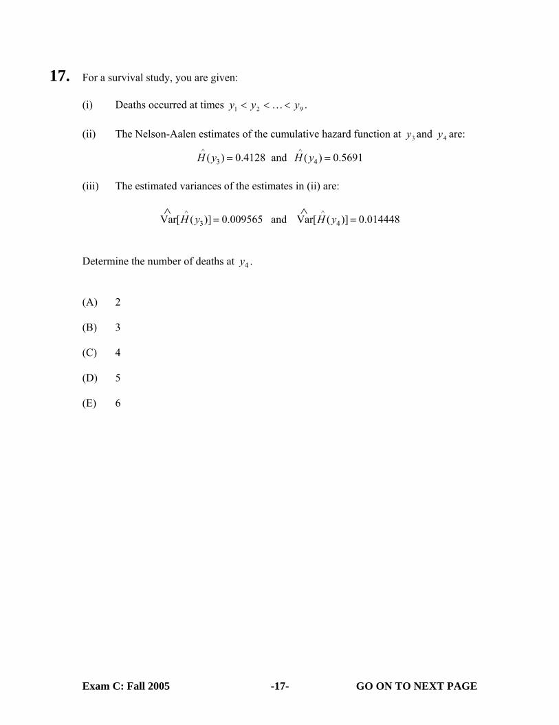
17. For a survival study, you are given: (i) Deaths occurred at times 921 yyy <<< … . (ii) The Nelson-Aalen estimates of the cumulative hazard function at 3y and 4y are:

^ ^3 4( ) 0.4128 and ( ) 0.5691H y H y= =

(iii) The estimated variances of the estimates in (ii) are:

^

3Var[ ( )] 0.009565 H y =∧

and ^

4Var[ ( )] 0.014448H y =∧

Determine the number of deaths at 4y . (A) 2 (B) 3 (C) 4 (D) 5 (E) 6


18. A random sample of size n is drawn from a distribution with probability density function:

2( ) , 0 , 0( )

f x xx

θ θθ

= < < ∞ >+

Determine the asymptotic variance of the maximum likelihood estimator of θ .

(A) n23θ

(B) 231θn

(C) 23

nθ

(D) 23nθ

(E) 231θ


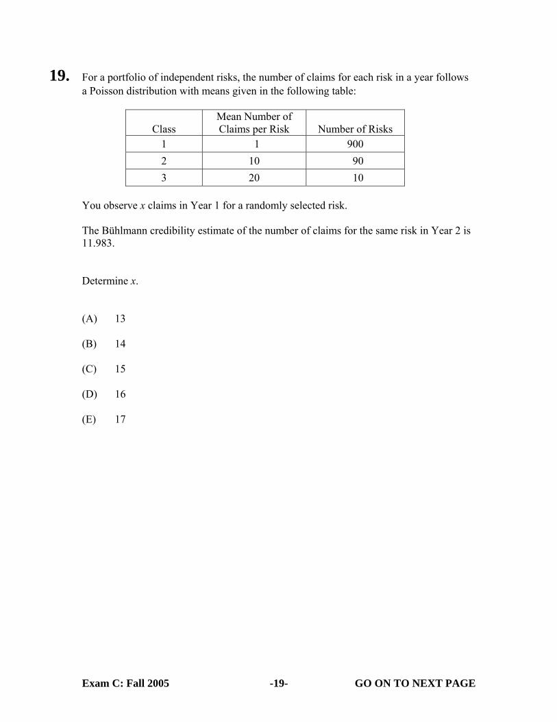
19. For a portfolio of independent risks, the number of claims for each risk in a year follows a Poisson distribution with means given in the following table:

Class Mean Number of Claims per Risk Number of Risks

1 1 900 2 10 90 3 20 10

You observe x claims in Year 1 for a randomly selected risk. The Bühlmann credibility estimate of the number of claims for the same risk in Year 2 is 11.983. Determine x. (A) 13

(B) 14

(C) 15

(D) 16

(E) 17


20. A survival study gave (0.283, 1.267) as the symmetric linear 95% confidence interval for H(5). Using the delta method, determine the symmetric linear 95% confidence interval for S(5). (A) (0.23, 0.69) (B) (0.26, 0.72) (C) (0.28, 0.75) (D) (0.31, 0.73) (E) (0.32, 0.80)


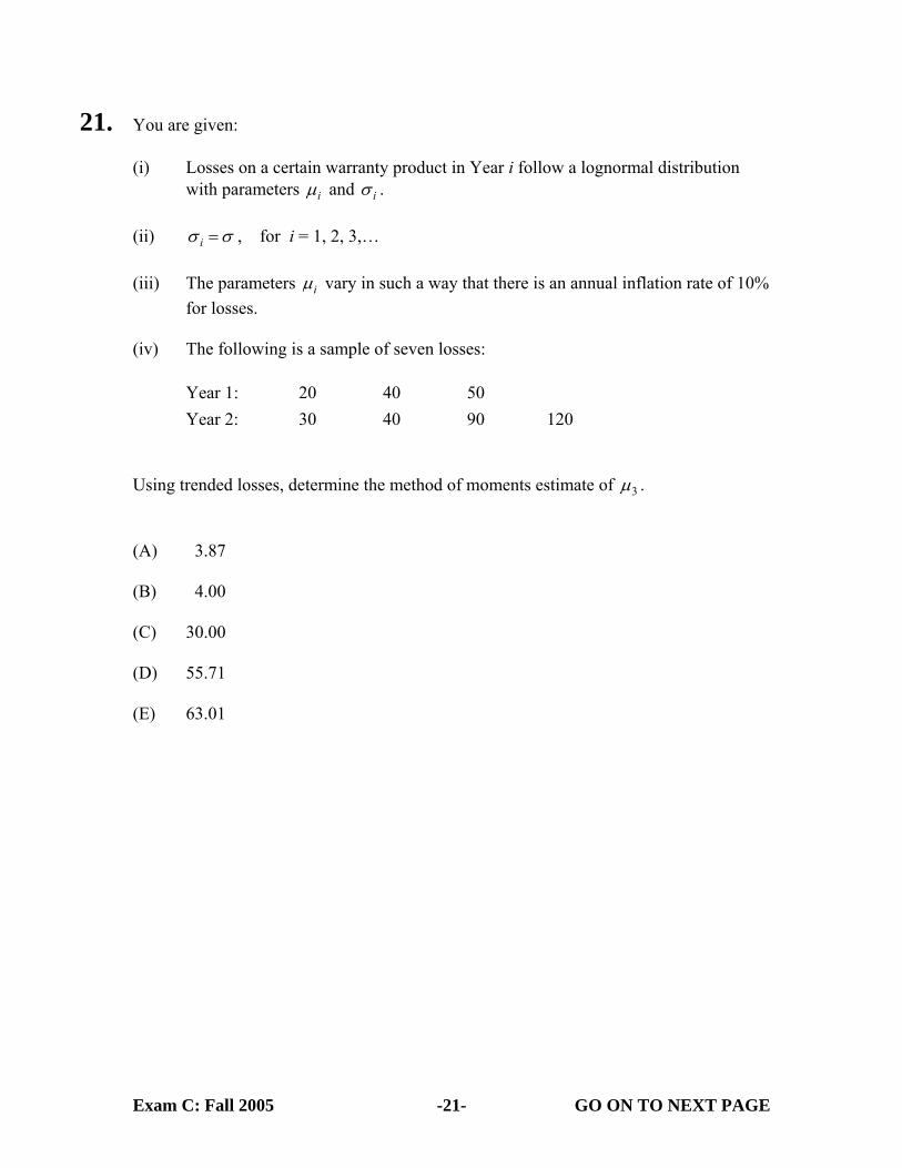
21. You are given: (i) Losses on a certain warranty product in Year i follow a lognormal distribution

with parameters iµ and iσ .

(ii) iσ σ= , for i = 1, 2, 3,…

(iii) The parameters iµ vary in such a way that there is an annual inflation rate of 10% for losses.

(iv) The following is a sample of seven losses:

Year 1: 20 40 50 Year 2: 30 40 90 120

Using trended losses, determine the method of moments estimate of 3µ . (A) 3.87

(B) 4.00

(C) 30.00

(D) 55.71

(E) 63.01


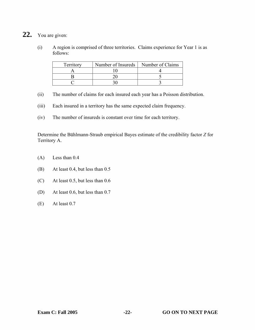
22. You are given: (i) A region is comprised of three territories. Claims experience for Year 1 is as

follows:

Territory Number of Insureds Number of Claims A 10 4 B 20 5 C 30 3

(ii) The number of claims for each insured each year has a Poisson distribution. (iii) Each insured in a territory has the same expected claim frequency. (iv) The number of insureds is constant over time for each territory. Determine the Bühlmann-Straub empirical Bayes estimate of the credibility factor Z for Territory A. (A) Less than 0.4 (B) At least 0.4, but less than 0.5 (C) At least 0.5, but less than 0.6 (D) At least 0.6, but less than 0.7 (E) At least 0.7


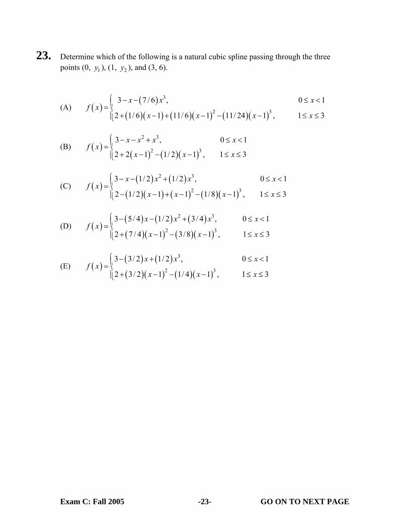
23. Determine which of the following is a natural cubic spline passing through the three points (0, 1y ), (1, 2y ), and (3, 6).

(A) ( )( )

( )( ) ( )( ) ( )( )

3

2 3

3 7 / 6 , 0 1

2 1/ 6 1 11/ 6 1 11/ 24 1 , 1 3

x x xf x

x x x x

⎧ − − ≤ <⎪= ⎨+ − + − − − ≤ ≤⎪⎩

(B) ( )( ) ( )( )

2 3

2 3

3 , 0 1

2 2 1 1/ 2 1 , 1 3

x x x xf x

x x x

⎧ − − + ≤ <⎪= ⎨+ − − − ≤ ≤⎪⎩

(C) ( )( ) ( )

( )( ) ( ) ( )( )

2 3

2 3

3 1/ 2 1/ 2 , 0 1

2 1/ 2 1 1 1/8 1 , 1 3

x x x xf x

x x x x

⎧ − − + ≤ <⎪= ⎨− − + − − − ≤ ≤⎪⎩

(D) ( )( ) ( ) ( )( )( ) ( )( )

2 3

2 3

3 5/ 4 1/ 2 3/ 4 , 0 1

2 7 / 4 1 3/8 1 , 1 3

x x x xf x

x x x

⎧ − − + ≤ <⎪= ⎨+ − − − ≤ ≤⎪⎩

(E) ( )( ) ( )( )( ) ( )( )

3

2 3

3 3/ 2 1/ 2 , 0 1

2 3/ 2 1 1/ 4 1 , 1 3

x x xf x

x x x

⎧ − + ≤ <⎪= ⎨+ − − − ≤ ≤⎪⎩


24. You are given: (i) A Cox proportional hazards model was used to study the survival times of

patients with a certain disease from the time of onset to death. (ii) A single covariate z was used with z = 0 for a male patient and z = 1 for a female

patient. (iii) A sample of five patients gave the following survival times (in months): Males: 10 18 25 Females: 15 21 (iv) The parameter estimate is β = 0.27. Using the Nelson-Aalen estimate of the baseline cumulative hazard function, estimate the probability that a future female patient will survive more than 20 months from the time of the onset of the disease. (A) 0.33 (B) 0.36

(C) 0.40

(D) 0.43 (E) 0.50


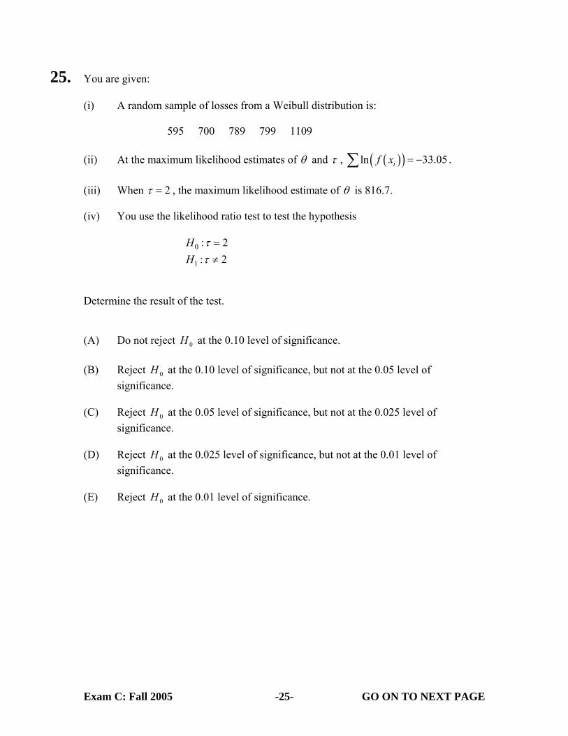
25. You are given: (i) A random sample of losses from a Weibull distribution is:

595 700 789 799 1109 (ii) At the maximum likelihood estimates of θ and τ , ( )( )ln 33.05if x = −∑ .

(iii) When 2τ = , the maximum likelihood estimate of θ is 816.7.

(iv) You use the likelihood ratio test to test the hypothesis

0 : 2H τ =

1 : 2H τ ≠ Determine the result of the test. (A) Do not reject 0H at the 0.10 level of significance. (B) Reject 0H at the 0.10 level of significance, but not at the 0.05 level of

significance. (C) Reject 0H at the 0.05 level of significance, but not at the 0.025 level of

significance. (D) Reject 0H at the 0.025 level of significance, but not at the 0.01 level of

significance. (E) Reject 0H at the 0.01 level of significance.


26. For each policyholder, losses X1,…, Xn , conditional on Θ, are independently and identically distributed with mean,

( ) ( )E , 1,2,...,jX j nµ θ θ= Θ = =

and variance,

( ) ( )Var , 1,2,...,jv X j nθ θ= Θ = = .

You are given:

(i) The Bühlmann credibility assigned for estimating X5 based on X1,…, X4 is Z = 0.4.

(ii) The expected value of the process variance is known to be 8. Calculate ( )Cov ,i jX X , i j≠ . (A) Less than 0.5− (B) At least 0.5− , but less than 0.5 (C) At least 0.5, but less than 1.5 (D) At least 1.5, but less than 2.5 (E) At least 2.5


27. Losses for a warranty product follow the lognormal distribution with underlying normal mean and standard deviation of 5.6 and 0.75 respectively. You use simulation to estimate claim payments for a number of contracts with different deductibles. The following are four uniform (0,1) random numbers:

0.6217 0.9941 0.8686 0.0485 Using these numbers and the inversion method, calculate the average payment per loss for a contract with a deductible of 100. (A) Less than 630

(B) At least 630, but less than 680

(C) At least 680, but less than 730

(D) At least 730, but less than 780

(E) At least 780


28. The random variable X has the exponential distribution with mean θ . Calculate the mean-squared error of 2X as an estimator of 2θ . (A) 20 4θ (B) 21 4θ (C) 22 4θ (D) 23 4θ (E) 24 4θ


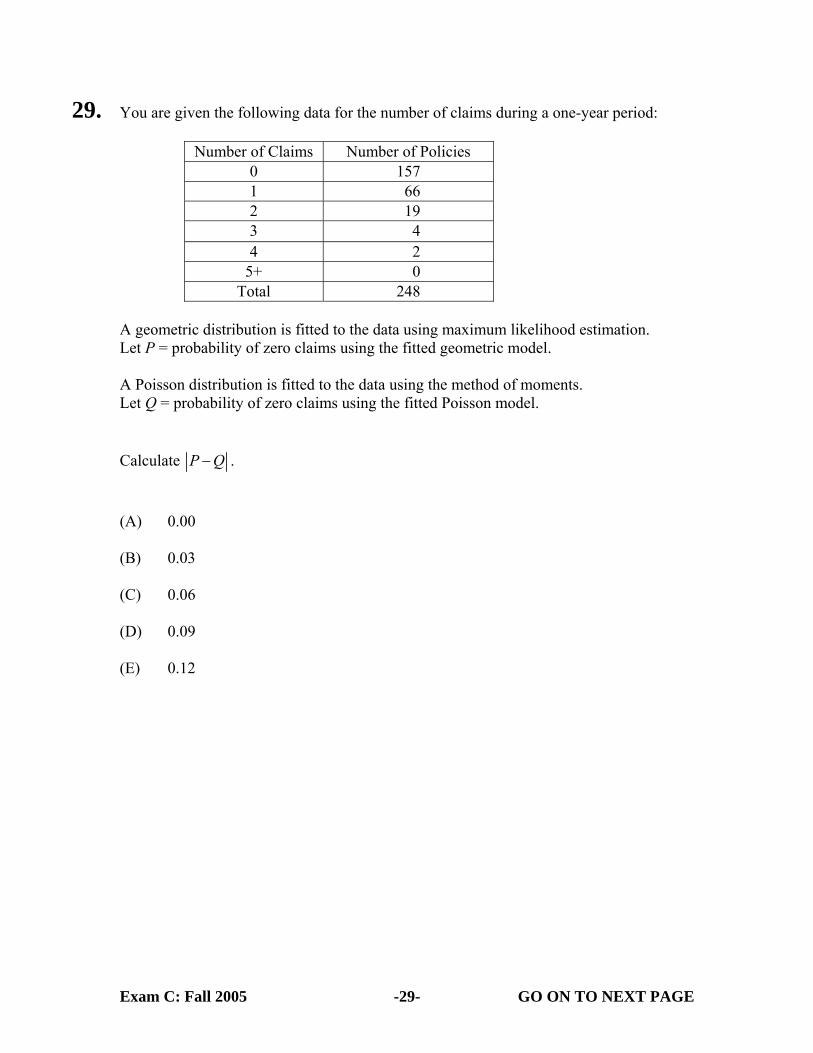
29. You are given the following data for the number of claims during a one-year period:

Number of Claims Number of Policies 0 157 1 66 2 19 3 4 4 2

5+ 0 Total 248

A geometric distribution is fitted to the data using maximum likelihood estimation. Let P = probability of zero claims using the fitted geometric model. A Poisson distribution is fitted to the data using the method of moments. Let Q = probability of zero claims using the fitted Poisson model. Calculate P Q− . (A) 0.00 (B) 0.03 (C) 0.06 (D) 0.09 (E) 0.12


30. For a group of auto policyholders, you are given: (i) The number of claims for each policyholder has a conditional Poisson

distribution. (ii) During Year 1, the following data are observed for 8000 policyholders:

Number of Claims Number of Policyholders 0 5000 1 2100 2 750 3 100 4 50

5+ 0 A randomly selected policyholder had one claim in Year 1. Determine the semiparametric empirical Bayes estimate of the number of claims in Year 2 for the same policyholder. (A) Less than 0.15 (B) At least 0.15, but less than 0.30 (C) At least 0.30, but less than 0.45 (D) At least 0.45, but less than 0.60 (E) At least 0.60


31. You are given: (i) The following are observed claim amounts:

400 1000 1600 3000 5000 5400 6200 (ii) An exponential distribution with 3300θ = is hypothesized for the data.

(iii) The goodness of fit is to be assessed by a p-p plot and a D(x) plot. Let (s, t) be the coordinates of the p-p plot for a claim amount of 3000. Determine ( ) ( )3000s t D− − . (A) −0.12 (B) −0.07 (C) 0.00 (D) 0.07 (E) 0.12


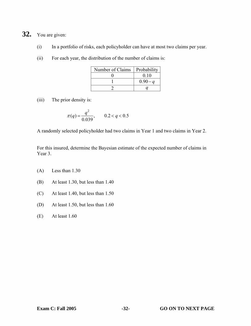
32. You are given: (i) In a portfolio of risks, each policyholder can have at most two claims per year. (ii) For each year, the distribution of the number of claims is:

Number of Claims Probability0 0.10 1 0.90 q− 2 q

(iii) The prior density is:

2( ) , 0.2 0.5

0.039qq qπ = < <

A randomly selected policyholder had two claims in Year 1 and two claims in Year 2. For this insured, determine the Bayesian estimate of the expected number of claims in Year 3. (A) Less than 1.30 (B) At least 1.30, but less than 1.40 (C) At least 1.40, but less than 1.50 (D) At least 1.50, but less than 1.60 (E) At least 1.60


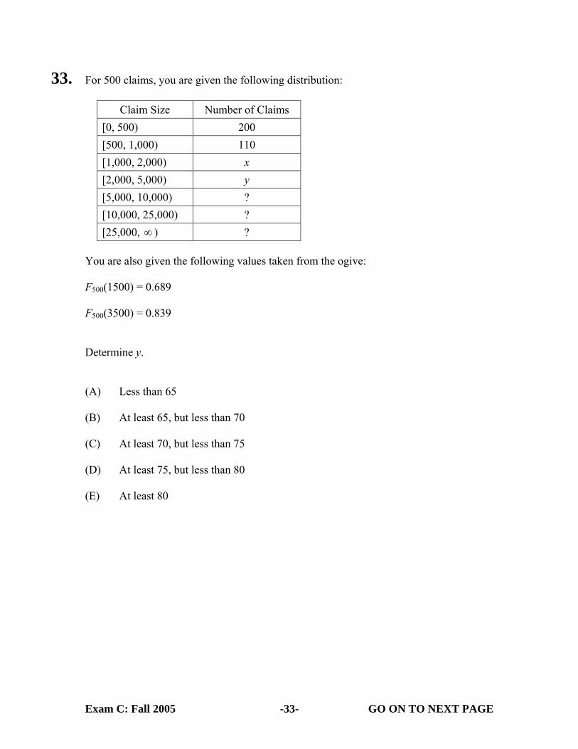
33. For 500 claims, you are given the following distribution:

Claim Size Number of Claims [0, 500) 200 [500, 1,000) 110 [1,000, 2,000) x [2,000, 5,000) y [5,000, 10,000) ? [10,000, 25,000) ? [25,000, ∞ ) ?

You are also given the following values taken from the ogive: F500(1500) = 0.689 F500(3500) = 0.839 Determine y. (A) Less than 65 (B) At least 65, but less than 70 (C) At least 70, but less than 75 (D) At least 75, but less than 80 (E) At least 80


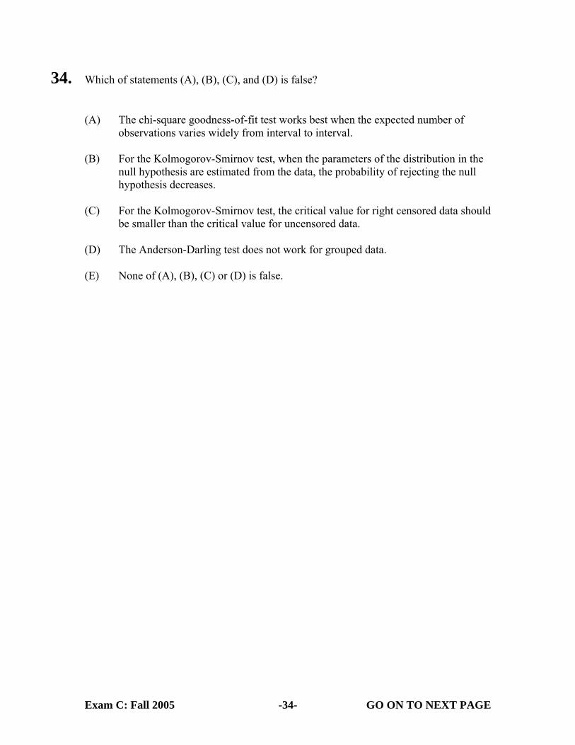
34. Which of statements (A), (B), (C), and (D) is false? (A) The chi-square goodness-of-fit test works best when the expected number of

observations varies widely from interval to interval. (B) For the Kolmogorov-Smirnov test, when the parameters of the distribution in the

null hypothesis are estimated from the data, the probability of rejecting the null hypothesis decreases.

(C) For the Kolmogorov-Smirnov test, the critical value for right censored data should

be smaller than the critical value for uncensored data. (D) The Anderson-Darling test does not work for grouped data. (E) None of (A), (B), (C) or (D) is false.

Exam C: Fall 2005 -35- STOP

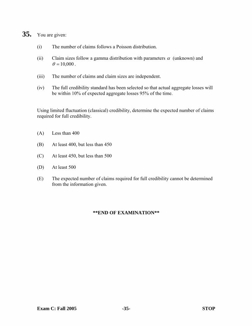
35. You are given: (i) The number of claims follows a Poisson distribution. (ii) Claim sizes follow a gamma distribution with parameters α (unknown) and

000,10=θ .

(iii) The number of claims and claim sizes are independent. (iv) The full credibility standard has been selected so that actual aggregate losses will

be within 10% of expected aggregate losses 95% of the time. Using limited fluctuation (classical) credibility, determine the expected number of claims required for full credibility. (A) Less than 400 (B) At least 400, but less than 450 (C) At least 450, but less than 500 (D) At least 500 (E) The expected number of claims required for full credibility cannot be determined

from the information given.

**END OF EXAMINATION**

FALL 2005 EXAM C SOLUTIONS

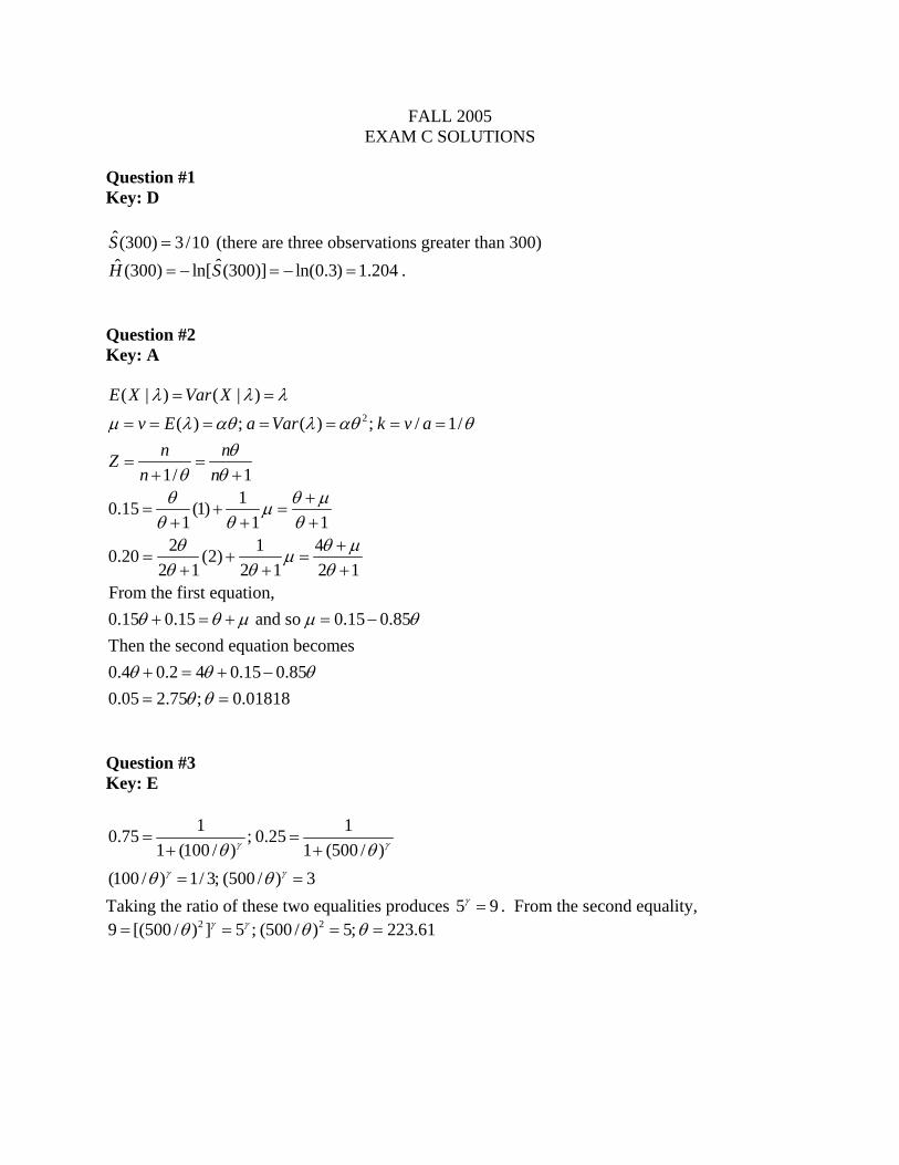
Question #1 Key: D ˆ(300) 3/10S = (there are three observations greater than 300)

ˆˆ (300) ln[ (300)] ln(0.3) 1.204H S= − = − = . Question #2 Key: A

2

( | ) ( | )( ) ; ( ) ; / 1/

1/ 110.15 (1)

1 1 12 1 40.20 (2)

2 1 2 1 2 1From the first equation,0.15 0.15 and so 0.15 0.85Then the second equat

E X Var Xv E a Var k v a

n nZn n

λ λ λ

µ λ αθ λ αθ θθ

θ θθ θ µµ

θ θ θθ θ µµ

θ θ θ

θ θ µ µ θ

= =

= = = = = = =

= =+ +

+= + =

+ + ++

= + =+ + +

+ = + = −ion becomes

0.4 0.2 4 0.15 0.850.05 2.75 ; 0.01818

θ θ θθ θ

+ = + −= =

Question #3 Key: E

1 10.75 ; 0.251 (100 / ) 1 (500 / )

(100 / ) 1/ 3; (500 / ) 3

γ γ

γ γ

θ θθ θ

= =+ +

= =

Taking the ratio of these two equalities produces 5 9γ = . From the second equality, 2 29 [(500 / ) ] 5 ; (500 / ) 5; 223.61γ γθ θ θ= = = =

Question #4 Key: B

2 3( )0 (0)2 (2) 2 4 81 '(0)

24 ''(2) 2 12 ; 12 6

f x a bx cx dxf af a b c df b

f c d c d

= + + += == = + + += =− = = + = − −

Insert the values for a, b, and c into the second equation to obtain 2 2 4( 12 6 ) 8 ; 48 16 ; 3d d d d= + − − + = − = − Then 6c = and 2 3( ) 6 3 ; (1) 4f x x x x f= + − = Question #5 Key: E Begin with

y 350 500 1000 1200 1500s 2 2 1 1 1 r 10 8 5 2 1

Then 18 6 4 1ˆ (1250) 0.24

10 8 5 2S = =

The likelihood function is 2 2 21 350/ 1 500/ 500/ 1 1000/ 1000/ 1 1200/ 1 1500/

7 7900/

2

1250(7) / 79002

( )

7900 7 7900 ˆ( ) 7 ln ; '( ) 0; 7900 / 7

ˆ (1250) 0.33

L e e e e e e e

e

l l

S e

θ θ θ θ θ θ θ

θ

θ θ θ θ θ θ

θ

θ θ θ θθ θ θ

− − − − − − − − − − − −

− −

−

⎡ ⎤ ⎡ ⎤ ⎡ ⎤= ⎣ ⎦ ⎣ ⎦ ⎣ ⎦=

= − − = − + = =

= =

The absolute difference is 0.09.

Question #6 Key: E

4

2 2 3

4 4 4 12

2 2 3 2 2 3 2 2 2 2 3 2 5

2 2

4 2 4 2 42 2

4( ) '( )( )

4(2) 4(4) 128( ) (2) (4) (4)( 2 ) ( 4 ) ( 4 ) ( 4) ( 16)

( ) ln128 12ln 3ln( 4) 5ln( 16)12 6 10'( ) 0;12( 20 64) 6( 16 ) 10( 4

4 16

xf x S xx

L f f S

l

l

θθ

θ θ θ θθθ θ θ θ θ

θ θ θ θθ θθ θ θ θ θ θ

θ θ θ

= − =+

= = =+ + + + +

= + − + − +

= − − = + + − + − ++ +

2

4 2 4 2

22

) 0

0 4 104 768 26 192

26 26 4(192)32; 5.657

2

θ

θ θ θ θ

θ θ

=

= − + + = − −

± += = =

Question #7 Key: A

2 2 2 22

2 20 0

1 4

012 5

0

2 2

2 2 2 4 4( | ) ; ( | )3 9 2 9 18

(2 / 3) ( ) (2 / 3) 4 8 /15

(1/18) ( ) (1/18) 4 1/ 27

(2 / 3) ( ) (4 / 9) 4 / 6 (4 / 5) 8 / 675

1/ 27 125 / 8;8 / 675 1 25 / 8

x xE X x dx Var X x dx

E d

EVPV v E d

VHM a Var

k Z

θ θθ θ θ θ θθ θθ θ

µ θ θ θ

θ θ θ

θ

= = = − = − =

= = =

= = = =

⎡ ⎤= = = − =⎣ ⎦

= = = =+

∫ ∫

∫∫

8 / 33

Estimate is (8 / 33)(0.1) (25 / 33)(8 /15) 0.428.+ =

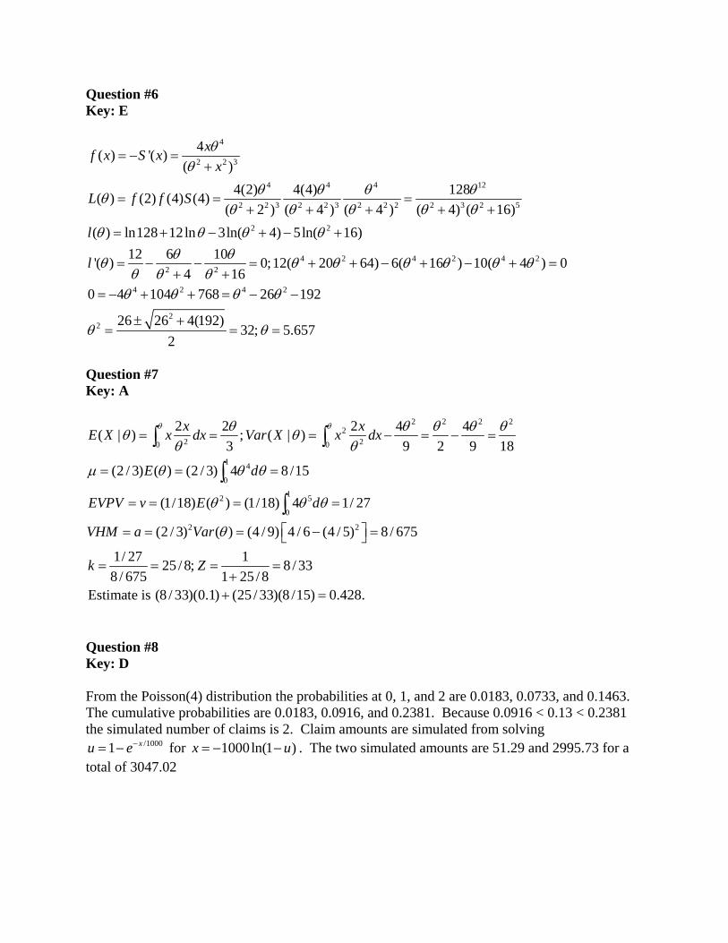
Question #8 Key: D From the Poisson(4) distribution the probabilities at 0, 1, and 2 are 0.0183, 0.0733, and 0.1463. The cumulative probabilities are 0.0183, 0.0916, and 0.2381. Because 0.0916 < 0.13 < 0.2381 the simulated number of claims is 2. Claim amounts are simulated from solving

/10001 xu e−= − for 1000ln(1 )x u= − − . The two simulated amounts are 51.29 and 2995.73 for a total of 3047.02

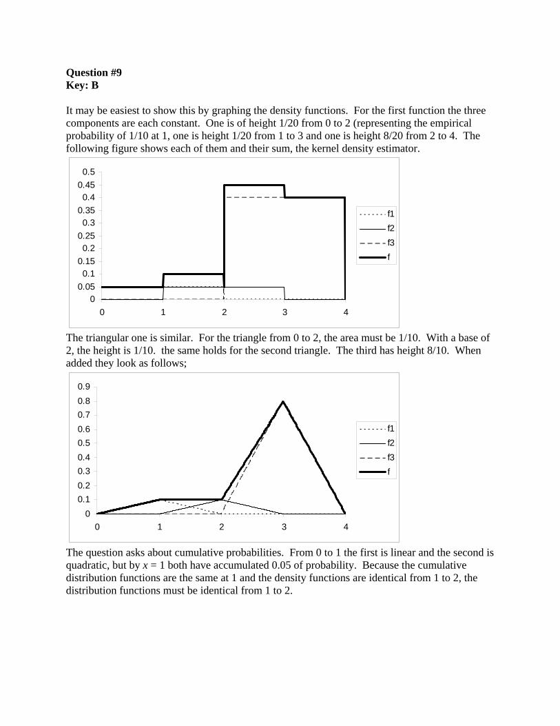
Question #9 Key: B It may be easiest to show this by graphing the density functions. For the first function the three components are each constant. One is of height 1/20 from 0 to 2 (representing the empirical probability of 1/10 at 1, one is height 1/20 from 1 to 3 and one is height 8/20 from 2 to 4. The following figure shows each of them and their sum, the kernel density estimator.

00.050.1

0.150.2

0.250.3

0.350.4

0.450.5

0 1 2 3 4

f1f2f3f

The triangular one is similar. For the triangle from 0 to 2, the area must be 1/10. With a base of 2, the height is 1/10. the same holds for the second triangle. The third has height 8/10. When added they look as follows;

00.10.20.30.40.50.60.70.80.9

0 1 2 3 4

f1f2f3f

The question asks about cumulative probabilities. From 0 to 1 the first is linear and the second is quadratic, but by x = 1 both have accumulated 0.05 of probability. Because the cumulative distribution functions are the same at 1 and the density functions are identical from 1 to 2, the distribution functions must be identical from 1 to 2.

Question #10 Key: D and E For the Poisson distribution, the mean, λ, is estimated as 230/1000 = 0.23. # of Days Poisson

Probability Expected # of Workers

Observed # of Workers

χ2

0 0.794533 794.53 818 0.69 1 0.182743 182.74 153 4.84 2 0.021015 21.02 25 0.75 3 or more 0.001709 1.71 4 3.07 Total 1000 9.35 The χ2 distribution has 2 degrees of freedom because there are four categories and the Poisson parameter is estimated (d.f. = 4 – 1 – 1 = 2).

The critical values for a chi-square test with two degrees of freedom are shown in the following table.

Significance Level Critical Value

10% 4.61 5% 5.99

2.5% 7.38 1% 9.21

9.35 is greater than 9.21 so the null hypothesis is rejected at the 1% significance level. Question #11 Key: D

2 225(480 472.73) 30(466.67 472.73)ˆ 2423.032 1

EVPV v − + −= = =

− where 480 = 12,000/25,

466.67 = 14,000/30, and 472.73 = 26,000/55. 552423.03/ 254 9.54; 0.852

55 9.54k Z= = = =

+

Question #12 Key: C

1.6 , 0 1''( )

1.6 0.8( 1) 2.4 0.8 , 1 2x x

f xx x x

< <⎧= ⎨ − − = − < <⎩

1 22 2

0 1(1.6 ) (2.4 0.8 ) 2.56S x dx x dx= + − =∫ ∫

Question #13 Key: C Relative risk = 1 2e β β− − which has partial derivatives 0.2e−− at 1 0.05β = and 2

ˆ 0.15β = Using the delta method, the variance of the relative risk is

( )0.2 0.4

0.2 0.20.2

2 11 7 0.0004691 310,000 10,000

e ee ee

− −− −

−

⎛ ⎞−⎛ ⎞− − = =⎜ ⎟⎜ ⎟⎜ ⎟−⎝ ⎠⎝ ⎠

Std dev = 0.0217 upper limit = ( )0.2 1.96 0.0217e− + = 0.8613 Alternatively, consider the quantity 1 2β β+ . The variance is

( )2 1 11 71 1 0.00071 3 110,000 10,000⎛ ⎞⎛ ⎞

= =⎜ ⎟⎜ ⎟⎝ ⎠⎝ ⎠

. The lower limit for this quantity is

0.2 1.96 0.0007 0.1481− = and the upper limit for the relative risk is 0.1481 0.8623e− = . Question #14 Key: C

The quantity of interest is ln 5000Pr( 5000)P X µσ

−⎛ ⎞= ≤ = Φ⎜ ⎟⎝ ⎠

. The point estimate is

ln 5000 6.84 (1.125) 0.871.49

−⎛ ⎞Φ = Φ =⎜ ⎟⎝ ⎠

.

For the delta method: (1.125) 1.125 (1.125)0.1422; 0.16001.49 1.49

P Pφ φµ σ∂ − ∂ −

= = − = = −∂ ∂

where 2 / 21( )

2zz eφ

π−= .

Then the variance of P is estimated as 2 2( 0.1422) 0.0444 ( 0.16) 0.0222 0.001466− + − = and the lower limit is 0.87 1.96 0.001466 0.79496LP = − = .

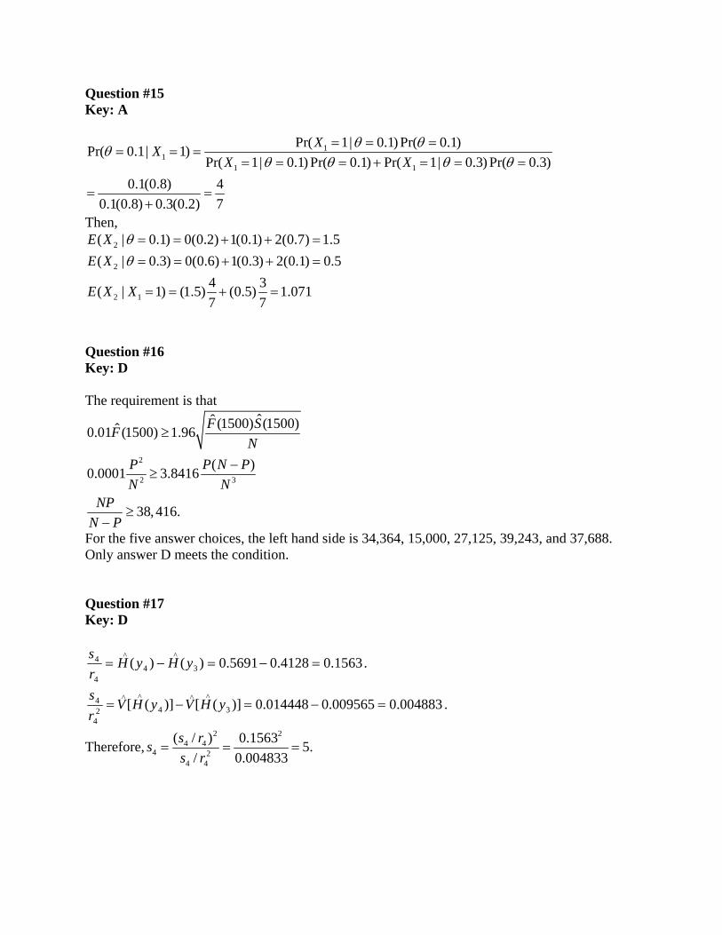
Question #15 Key: A

11

1 1

Pr( 1| 0.1) Pr( 0.1)Pr( 0.1| 1)Pr( 1| 0.1) Pr( 0.1) Pr( 1| 0.3) Pr( 0.3)

0.1(0.8) 40.1(0.8) 0.3(0.2) 7

XXX X

θ θθθ θ θ θ

= = == = =

= = = + = = =

= =+

Then, 2

2

2 1

( | 0.1) 0(0.2) 1(0.1) 2(0.7) 1.5( | 0.3) 0(0.6) 1(0.3) 2(0.1) 0.5

4 3( | 1) (1.5) (0.5) 1.0717 7

E XE X

E X X

θθ= = + + == = + + =

= = + =

Question #16 Key: D The requirement is that

2

2 3

ˆˆ (1500) (1500)ˆ0.01 (1500) 1.96

( )0.0001 3.8416

38,416.

F SFN

P P N PN N

NPN P

≥

−≥

≥−

For the five answer choices, the left hand side is 34,364, 15,000, 27,125, 39,243, and 37,688. Only answer D meets the condition. Question #17 Key: D

1563.04128.05691.0)()( 3^

4^

4

4 =−=−= yHyHrs .

004883.0009565.0014448.0)]([)]([ 3^^

4^^

24

4 =−=−= yHVyHVrs .

Therefore,2 2

4 44 2

4 4

( / ) 0.1563 5./ 0.004833

s rss r

= = =

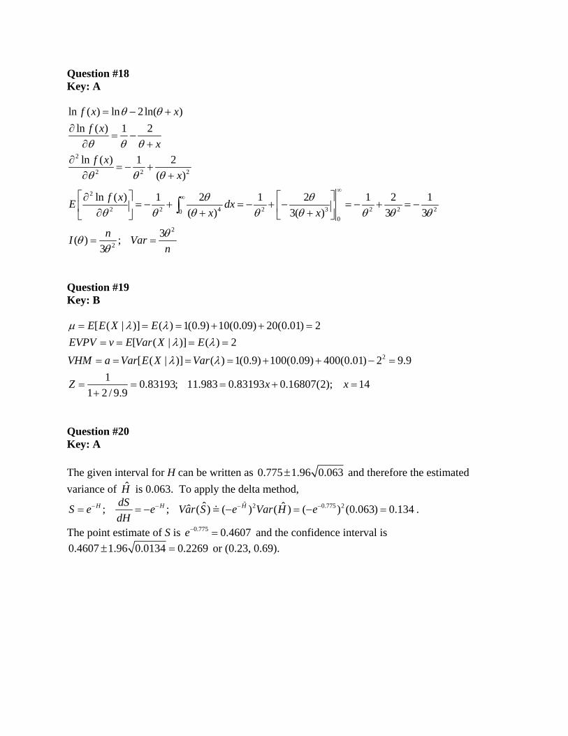
Question #18 Key: A

2

2 2 2

2

2 2 4 2 3 2 2 200

2

2

ln ( ) ln 2 ln( )ln ( ) 1 2

ln ( ) 1 2( )

ln ( ) 1 2 1 2 1 2 1( ) 3( ) 3 3

3( ) ;3

f x xf x

xf x

x

f xE dxx x

nI Varn

θ θ

θ θ θ

θ θ θ

θ θθ θ θ θ θ θ θ θ

θθθ

∞∞

= − +∂

= −∂ +

∂= − +

∂ +

⎡ ⎤ ⎡ ⎤∂= − + = − + − = − + = −⎢ ⎥ ⎢ ⎥∂ + +⎣ ⎦⎣ ⎦

= =

∫

Question #19 Key: B

2

[ ( | )] ( ) 1(0.9) 10(0.09) 20(0.01) 2[ ( | )] ( ) 2[ ( | )] ( ) 1(0.9) 100(0.09) 400(0.01) 2 9.9

1 0.83193; 11.983 0.83193 0.16807(2); 141 2 / 9.9

E E X EEVPV v E Var X EVHM a Var E X Var

Z x x

µ λ λλ λ

λ λ

= = = + + == = = =

= = = = + + − =

= = = + =+

Question #20 Key: A The given interval for H can be written as 0.775 1.96 0.063± and therefore the estimated variance of H is 0.063. To apply the delta method,

ˆ 2 0.775 2ˆ ˆˆ; ; ( ) ( ) ( ) ( ) (0.063) 0.134H H HdSS e e Var S e Var H edH

− − − −= = − − = − = .

The point estimate of S is 0.775 0.4607e− = and the confidence interval is 0.4607 1.96 0.0134 0.2269± = or (0.23, 0.69).

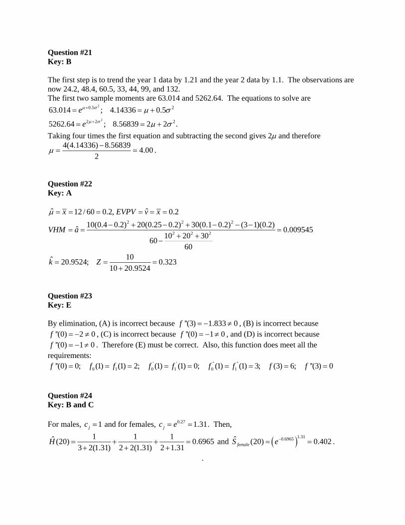
Question #21 Key: B The first step is to trend the year 1 data by 1.21 and the year 2 data by 1.1. The observations are now 24.2, 48.4, 60.5, 33, 44, 99, and 132. The first two sample moments are 63.014 and 5262.64. The equations to solve are

2

2

0.5 2

2 2 2

63.014 ; 4.14336 0.5

5262.64 ; 8.56839 2 2 .

e

e

µ σ

µ σ

µ σ

µ σ

+

+

= = +

= = +

Taking four times the first equation and subtracting the second gives 2µ and therefore 4(4.14336) 8.56839 4.00

2µ −= = .

Question #22 Key: A

2 2 2

2 2 2

ˆ ˆ12 / 60 0.2, 0.210(0.4 0.2) 20(0.25 0.2) 30(0.1 0.2) (3 1)(0.2)ˆ 0.009545

10 20 306060

10ˆ 20.9524; 0.32310 20.9524

x EVPV v x

VHM a

k Z

µ = = = = = =

− + − + − − −= = =

+ +−

= = =+

Question #23 Key: E By elimination, (A) is incorrect because ''(3) 1.833 0f = − ≠ , (B) is incorrect because

''(0) 2 0f = − ≠ , (C) is incorrect because ''(0) 1 0f = − ≠ , and (D) is incorrect because ''(0) 1 0f = − ≠ . Therefore (E) must be correct. Also, this function does meet all the

requirements: ' ' '' ''

0 1 0 1 0 1''(0) 0; (1) (1) 2; (1) (1) 0; (1) (1) 3; (3) 6; ''(3) 0f f f f f f f f f= = = = = = = = = Question #24 Key: B and C For males, 1jc = and for females, 0.27 1.31jc e= = . Then,

1 1 1ˆ (20) 0.69653 2(1.31) 2 2(1.31) 2 1.31

H = + + =+ + +

and ( )1.310.6965ˆ (20) 0.402femaleS e−= = .

.

Question #25 Key: C

5 5

1 1

( , ) ln ( ) ln ( 1) ln ln ( / )j j jj j

l f x x x ττ θ τ τ τ θ θ= =

= = + − − −∑ ∑ . Under the null hypothesis it is

52

1

(2, ) ln 2 ln 2ln ( / )j jj

l x xθ θ θ=

= + − −∑ . Inserting the maximizing value of 816.7 for θ gives

35.28− . The likelihood ratio test statistic is 2( 33.05 35.28) 4.46− + = . There is one degree of freedom. At a 5% significance level the critical value is 3.84 and at a 2.5% significance level it is 5.02. Question #26 Key: C

It is given that n = 4, v = 8, and Z = 0.4. Then, 40.4 84a

=+

which solves for a = 4/3. For the

covariance,

2 2

( , ) ( ) ( ) ( )

[ ( | )] [ ( | )] [ ( | )]

[ ( ) ] [ ( )] [ ( )] 4 / 3.

i j i j i j

i j i j

Cov X X E X X E X E X

E E X X E E X E E X

E E Var a

θ θ θ

µ θ µ θ µ θ

= −

= −

= − = = =

Question #27 Key: A

u z x lognormal with deductible 0.6217 0.31 5.8325 341.21 241.21 0.9941 2.52 7.49 1790.05 1690.05 0.8686 1.12 6.44 626.41 526.41 0.0485 −1.66 4.355 77.87 0

Average 614.42 The value of z is obtained by inversion from the standard normal table. That is, Pr( )u Z z= ≤ . The value of x is obtained from 0.75 5.6x z= + . The lognormal value is obtained by exponentiating x and the final column applies the deductible.

Question #28 Key: B

2 2 2 4 2 2 4

4 2 2 4 4

[( ) ] ( 2 )24 2(2 ) 21

MSE E X E X Xθ θ θ

θ θ θ θ θ

= − = − +

= − + =

Question #29 Key: C

The sample mean of 157(0) 66(1) 19(2) 4(3) 2(4) 0.5248

+ + + += is the maximum likelihood

estimate of the geometric parameter β as well as the method of moments estimate of the Poisson parameter λ. Then, 1(1 0.5) 0.6667P −= + = and 0.5 0.6065Q e−= = . The absolute difference is 0.0602. Question #30 Key: D

5000(0) 2100(1) 750(2) 100(3) 50(4) 0.51258000

x + + + += = and

2 2 2 2 22 5000(0.5125) 2100(0.4875) 750(1.4875) 100(2.4875) 50(3.4875) 0.5874

7999s + + + += = .

Then, ˆ ˆ 0.5125v xµ = = = and 2ˆ 0.0749a s x= − = . The credibility factor is 1 0.1275

1 0.5125 / 0.0749Z = =

+ and the estimate is 0.1275(1) 0.8725(0.5125) 0.5747.+ =

Question #31 Key: B

(3000) 4 / 8 0.5ns F= = = because for the p-p plot the denominator is n+1. 3000/3300(3000) 1 0.59711t F e−= = − = . For the difference plot, D uses a denominator of n and so

4 / 7 0.59711 0.02568D = − = − and the answer is 0.5 0.59711 0.02568 0.071.− + = −

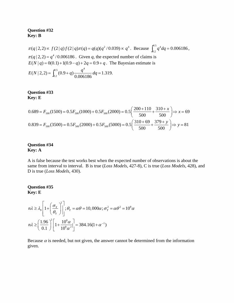
Question #32 Key: B

2 4( | 2, 2) (2 | ) (2 | ) ( ) ( )( / 0.039)q f q f q q q q q qπ π∝ = ∝ . Because 0.5 4

0.20.006186q dq =∫ ,

4( | 2, 2) / 0.006186q qπ = . Given q, the expected number of claims is ( | ) 0(0.1) 1(0.9 ) 2 0.9E N q q q q= + − + = + . The Bayesian estimate is

40.5

0.2( | 2, 2) (0.9 ) 1.319.

0.006186qE N q dq= + =∫

Question #33 Key: E

500 500 500200 110 3100.689 (1500) 0.5 (1000) 0.5 (2000) 0.5 69

500 500xF F F x+ +⎛ ⎞= = + = + ⇒ =⎜ ⎟

⎝ ⎠

500 500 500310 69 3790.839 (3500) 0.5 (2000) 0.5 (5000) 0.5 81

500 500yF F F y+ +⎛ ⎞= = + = + ⇒ =⎜ ⎟

⎝ ⎠

Question #34 Key: A A is false because the test works best when the expected number of observations is about the same from interval to interval. B is true (Loss Models, 427-8), C is true (Loss Models, 428), and D is true (Loss Models, 430). Question #35 Key: E

22 2 8

0

2 81

8 2

1 ; 10,000 ; 10

1.96 101 384.16(1 )0.1 10

YY Y

Y

n

n

σλ λ θ αθ α σ αθ αθ

αλ αα

−

⎡ ⎤⎛ ⎞⎢ ⎥≥ + = = = =⎜ ⎟⎢ ⎥⎝ ⎠⎣ ⎦

⎡ ⎤⎛ ⎞≥ + = +⎜ ⎟ ⎢ ⎥⎝ ⎠ ⎣ ⎦

Because α is needed, but not given, the answer cannot be determined from the information given.

exam c, fall 2005 final answer key

Documents