Examination of NERC GMD Standards and

Validation of Ground Models and Geo-Electric

Fields Proposed in this NERC GMD Standard

A White Paper by:

John G. Kappenman, Storm Analysis Consultants

and

Dr. Willam A. Radasky, Metatech Corporation

July 30, 2014

Executive Summary The analysis of the US electric power grid vulnerability to geomagnetic storms was originally conducted as part of the work performed by Metatech Corporation for the Congressional Appointed US EMP Commission, which started their investigations in late 2001. In subsequent work performed for the US Federal Energy Regulatory Commission, a detailed report was released in 2010 of the findings11. In October 2012, the FERC ordered the US electric power industry via their standards development organization NERC to develop new standards addressing the impacts of a geomagnetic disturbance to the electric power grid. NERC has now developed a draft standard and has provided limited details on the technical justifications for these standards in a recent NERC White Paper22. The most important purpose of design standards is to protect society from the consequences of impacts to vulnerable and critical systems important to society. To perform this function the standards must accurately describe the environment. Such environment design standards are used in all aspects of society to protect against severe excursions of nature that could impact vulnerable systems: floods, hurricanes, fire codes, etc., are relevant examples. In this case, an accurate characterization of the extremes of the geomagnetic storm environment needs to be provided so that power system vulnerabilities against these environments can be accurately assessed. A level that is arbitrarily too low would not allow proper assessment of vulnerability and ultimately would lead to inadequate safeguards that could pose broad consequences to society. However from our initial reviews of the NERC Draft Standard, the concern was that the levels suggested by NERC were unusually low compared to both recorded disturbances as well as from prior studies. Therefore this white paper will provide a more rigorous review of the NERC benchmark levels. NERC had noted that model validations were not undertaken because direct measurements of geo-electric fields had not been routinely performed anyway in the US. In contrast, Metatech had performed extensive geo-electric field measurement campaigns over decades for storms in Northern Minnesota and had developed validated models for many locations across the US in the course of prior investigations of US power grid vulnerability3. Further, various independent observers to the NERC GMD tasks force meetings had urged NERC to collect decades of GIC observations performed by EPRI and independently by power companies as these data could be readily converted to geo-electric fields via simple techniques to provide the basis for validation studies across the US. None of these actions were taken by the NERC GMD Task Force. It needs to be pointed out that GIC measurements are important witnesses and their evidence is not being considered by the NERC GMD Task Force in the development of these standards. GIC observations provide direct evidence of all of the uncertain and variable parameters including the deep Earth ground response to the driving geomagnetic disturbance environment. Because the GIC measurement is also obtained from the power grid itself, it incorporates all of the meso-scale coupling of the disturbance environments to the assets themselves and the overlying circuit topology that needs

1Geomagnetic Storms and Their Impacts on the U.S. Power Grid (Meta-R-319), John Kappenman, Metatech Corporation,

January 2010. Via weblink from Oak Ridge National Lab, wttp://www.ornl.gov/sci/ees/etsd/pes/ferc_emp_gic.shtml

2 NERC Benchmark Geomagnetic Disturbance Event Description,

http://www.nerc.com/pa/Stand/Project201303GeomagneticDisturbanceMitigation/Benchmark_GMD_Event_April21_2.pdf

3 Radasky, W. A., M. A. Messier, J. G. Kappenman, S. Norr and R. Parenteau, “Presentation and Analysis of

Geomagnetic Storm Signals at High Data Rates”, IEEE International Symposium on EMC, August 1993, pp. 156-

157.

to be assessed. Separate discreet measurements of geo-electric fields are usually done over short baseline asset arrays which may not accurately characterize the real meso-scale interdependencies that need to be understood. The only challenge is to interpret what the GIC measurement is attempting to tell us, and fortunately this can be readily revealed with only a rudimentary understanding of Ohm’s Law, geometry and circuit analysis methods, a tool set that are common electrical engineering techniques. Essentially the problem reduces to: “if we know the I (or GIC) and we know the R and topology of the circuit, then Ohm’s law tells us what the V or geo-electric field was that created that GIC”. Further since we know the resistance and locations of power system assets with high accuracy, we can also derive the geo-electric field with equally high certainty. These techniques allow superior characterization of deep Earth ground response and can be done immediately across much of the US if GIC measurements were made available. Further these deep Earth ground responses are based upon geological processes and do not change rapidly over time. Therefore even measurements from one storm event can characterize a region. Hence this is a powerful tool for improving the accuracy of models and allows for the development of accurate forward looking standards that are needed to evaluate to high storm intensity levels that have not been measured or yet experienced on present day power grids. Unfortunately this tool has not been utilized by any of the participants in the NERC Standard development process. It has been noted that the NERC GMD Task Force has adopted geo-electric field modelling techniques that have been previously developed at FMI and are now utilized at NRCan. The same FMI techniques were also integrated into the NASA-CCMC modeling environments and that as development and testing of US physiographic regional ground models were developed, efforts were also undertaken by the USGS and the NOAA SWPC to make sure their geo-electric field models were fully harmonized and able to produce uniform results. However, it appears that none of these organizations really did any analysis to determine if the results being produced were at all accurate in the first place. For example when recently inquired, NRCan indicated they will perhaps begin capturing geo-electric field measurements later this year to validate the base NERC Shield region ground model, a model which provides a conversion for all other ground models. In looking at prior publications of the geo-electric field model carried out in other world locations, it was apparent that the model was greatly and uniformly under-predicting for intense portions of the storms, which are the most important parameters that need to be accurately understood. In order to examine this more fully, this white paper will provide the results of our recent independent assessment of the NERC geo-electric field and ground models and the draft standard that flows from this foundation. Our findings can be concisely summarized as follows:

Using the very limited but publicly available GIC measurements, it can be shown how important geo-electric fields over meso-scale regions can be characterized and that these measurements can be accurately assessed using the certainty of Ohm’s Law. This provides a very strict constraint on what the minimum geo-electric field levels are during a storm event.

When comparing these actual geo-electric fields with NERC model derived geo-electric fields, the comparisons show a systematic under-prediction in all cases of the geo-electric field by the NERC model. In the cases examined, the under prediction is particularly a problem for the rapid rates of change of the geomagnetic field (the most important portions of the storm events) and produce errors that range from factor of ~2 to over factor of ~5 understatement of intensity by the NERC models compared to actual geo-electric field measurements. These are enormous errors and are not at all suitable to attempt to embed into Federally-approved design standards.

These enormous model errors also call into question many of the foundation findings of the NERC GMD draft standard. The flawed geo-electric field model was used to develop the peak geo-electric field levels of the Benchmark model proposed in the standard. Since this model understates the actual geo-electric field intensity for small storms by a factor of 2 to 5, it would also understate the maximum geo-electric field by similar or perhaps even larger levels. Therefore this flaw is entirely integrated into the NERC Draft Standard and its resulting directives are not valid and need to be corrected.

The findings here are also not simply a matter of whether the NERC model agrees with the results of the Metatech model. Rather the important issue is the degree that the NERC model disagrees with actual geo-electric field measurements from actual storm events. These actual measurements are also confirmed within very strict tolerances via Ohm’s Law, a fundamental law of nature. The results that the NERC model has provided are not reliable, and efforts by NERC to convince otherwise and that utilization of GIC data cannot be done are simply misplaced. Actual data provides an ultimate check on unverified models and can be more effectively utilized to guide standard development than models because as Richard Feynman once noted; “Nature cannot be fooled”!

Introduction to NERC Model Evaluation and Validation Overview A series of case study examples will be provided in this White Paper to illustrate the evaluation of geo-electric fields derived from GIC measurements across the US electric power grid. These derived geo-electric field results will then be compared to the NERC estimated geo-electric fields for the same storm events and scenarios. There are an important number of underlying principles to this analysis that can be summarized as follows:

Using past storms and by modeling detailed power networks and comparing to GIC measurements at particular locations is the best way to validate overall storm-phenomena/power grid models. It accounts for the "interpolation" of the incident measured B-fields (including the angular rotation of the fields with time), the accuracy of the ground model used, the coupling to the power network, and the computation of the current flow at the measurement point.

Experience has shown that over times of minutes, the geomagnetic field will rotate its direction and therefore every transformer in a network will have a sensitivity to particular vector orientations of the field, and the maximum current measured at a given transformer location will be a function of the rate of change intensity of the geomagnetic field, the resulting geo-electric field this causes and the angle of the field as it changes over the storm event. This is why the rate of change (dB/dt) and GIC at a single transformer will not scale perfectly with the maximum value of dB/dt, but taking into consideration all of these topology and orientation factors, a highly accurate forensic analysis can be performed.

Geomagnetic storms are not steady state events, rather they are events with aperiodic extreme impulsive disturbances that can occur over many hours or days duration. Modeling these events to derive a geo-electric field is challenging but readily achievable. Since these events are time domain problems, modeling solutions using time-domain methods are recommended. The NERC modeling methods that will be evaluated here have generally been developed using Fourier transform frequency domain methods. In these implementations of Fourier methods, the primary question is the accuracy in dealing with the phase of the Fourier transforms.

When referring to impulsive geomagnetic field disturbance events, these are typically multiple discrete events with times of several minutes. Note that the collapse of the Quebec power network in March 1989 occurred in 93 seconds. Clearly times of only a few minutes are important and it is vital that the geo-electric field intensity of these transients be accurately portrayed and not understated in a Design Standard type document. For example, a 10 meter dyke defined by the standard does no good, if the actual Tsunami height is 15 meters. Any efforts to claim that models that depict some satisfactory averaging over extended time periods as being sufficient must be vigorously refuted, as these peak inflection points are the most vital aspects of the storm environments that must be accurately determined.

Simulation Model Validation – Maine Grid Examples In the analysis carried out for the FERC Meta-R-319 report, extensive efforts were undertaken to verify that the simulation models for the US power grid were providing sufficiently accurate results. One of the primary approaches that were utilized to test these models were to perform simulations for forensic analysis purposes and to compare the results with discrete measurements that were available.

One of the forensic simulations was conducted on the Maine grid and provided important verification of the ability of the model in that portion of the US grid to produce accurate estimates. Figure 1 provides a plot of the results of this simulation showing the “Calculated” versus “Measured” GIC (geomagnetically induced current) at the Chester Maine 345kV transformer. This was for a storm which occurred on May 4, 1998 and was driven by the large scale storm conditions as shown in Figure 2.

Figure 1 – Plot showing comparison of Simulated versus Measured GIC at Chester Maine 345kV transformer for May 4,

1998 geomagnetic storm. (Source – Meta-R-319)

Figure 2 – Map of Geomagnetic Disturbance conditions at 4:16UT during May 4, 1998 storm. (Source – Meta-R-319)

The results in Figure 1 provide a comparison between high sample rate measured GIC (~10 second cadence) versus storm simulations that were limited to 1 minute cadence geomagnetic observatory data inputs (B-fields). Due to this limitation of inputs to the model, the model would not be able to reproduce all of the small scale high frequency variations shown in the measured data. However, the simulation does provide very good accuracy and agreement on major spikes in GIC observed, the most important portion of the simulation results that need to be validated. Figure 3 provides a wider view of the impact of the storm in terms of other GIC flow conditions in the Maine and New England region electric power grid, this is provided at time 4:16UT.

Figure 3 – GIC flows and disturbance conditions in Maine/New England grid at 4:16UT, May 4, 1998. (Source – Meta-R-

319)

As this illustration shows, the Chester GIC flow is shown along with comparable GIC flows in a number of other locations in the regional power grid at one minute in time. In addition to impacts to the New England grid, extensive power system impacts were also observed to voltage regulation in upstate New York region due to storm. In this map, the intensity and polarity of GIC flows are depicted by red or green balls and their size, the larger the ball the larger the GIC flow and the danger it presents to the transformer and grid. Also shown are the blue vector arrows which are the orientation and intensity of the geo-electric field which couples to the topology of the electric grid and produces the GIC flow patterns that develop in the grid. It is noted that during the period of this storm, the electric fields rotated and all transformers in the grid would experience a variation in the pattern of GIC flows. Considerable scientific and engineering examination has been performed since the release of the Meta-R-319 report; the report and other subsequent examinations are in close agreement on a number of

important parameters of future severe geomagnetic storm threat conditions. For example, it is now well-accepted that severe storm intensity disturbance intensity can reach level of 5000 nT/min at the latitudes of the Maine power grid. NRCan now provides estimates of geo-electric fields for the nearby Ottawa observatory for storms including the May 4, 1998 storm. The ability therefore exists to do cross-validations with this and other proposed NERC ground models and geo-electric field calculation methods. Observations of GIC at the Chester Maine substation also provide important observational confirmations that allow empirical projection of GIC levels that are plausible at more severe storm intensities. Earlier this year, the Maine electric utilities provided a limited summary of peak GIC observations from their Chester transformer and storm dates to the Maine Legislature. Figure 4 provides a graphical summary that was derived of the peak GIC and peak disturbance intensities (in nT/min) observed at the Ottawa Canada geomagnetic observatory for a number of reported events. The Maine utilities did not provide accurate time stamps (just date only), so that limits some of the ability to accurately correlate disturbance intensity to GIC peaks as the knowledge of timing is extremely coarse. Also since the Ottawa observatory is approximately 550km west of Chester, there is some uncertainty to local storm intensity specifics near Chester. However as shown, there are clear trend lines and uncertainty bounding of the level of GIC and how the GIC increases for increasing storm intensity. This trend line is quite revealing even with all of the previously mentioned uncertainties on the spatial and temporal aspects of the threat environments.

Figure 4 – GIC versus Storm Intensity (nT/min) from multiple observed GIC storm events at Chester Transformer, in

this case the GIC timing is extremely coarse.

At higher storm intensities, the geo-electric field increases and if only intensity changes (as opposed to spectral content), then the increase in geo-electric field and resulting GIC will be linear. Because storm

intensity for very severe storms can reach ~5000 nT/min, this graph can be linearly extended to project the range of GIC flows in the Chester transformer for these more extreme threat conditions. Figure 5 provides a plot similar to that in Figure 4, only with linear extensions of the GIC flow that this observational data estimates.

Figure 5 – Projected Chester GIC flow for storm intensity increasing to ~5000 nT/min.

Using these data plotting techniques with the previously noted uncertainties, a more detailed examination can be performed for one of the specific storm events which occurred on May 4, 1998. Figure 6 provides again the earlier described GIC plots from Figure 1. Two particularly important peak times are also highlighted on this plot at 4:16UT and 4:39UT where the recorded GIC reaches peaks respectively of -74.3 Amps and -66.6 Amps. These comparisons also show very close agreement with the simulation model results as well. Therefore the peak data points can be more explicitly examined in detail, as a comparison to how GIC vs dB/dt was plotted in Figure 4. In addition to this GIC observation data, there was also dB/dt data observed from a local magnetometer for this storm, which also greatly reduces the uncertainty of the threat environment. Having all of this data available will aid in utilizing the power system itself as an antenna that can help resolve the geo-electric field intensity that the complex composition of ground strata generates during this storm event. Further once this response is empirically established, this same ground response can be reliably utilized to project to higher storm intensity and therefore higher GIC levels. This provides a blended effort of model and observational data to extract details on how the same grid and ground strata would behave at higher storm intensity levels. One of the advantages that exists in the modeling of the circuits of the transmission networks are that the resistive impedances of transmission lines and transformers (which are the key GIC flow paths) are very well known and have small uncertainty errors. It is also known that the Chester transformer is non-auto, so GIC flow in the neutral also defines the GIC per phase. There is also no doubt about the locations of assets within the circuit topology. Finally, station grounding resistance can also be determined to relatively high certainty as well. In comparison,

ground response as has been previously published in the Meta-R-319 report can vary over large ranges, as much as a factor of 6. Therefore direct observations of ground response are highly important and GIC measurements, as will be discussed, provide an excellent proxy or geophysical data that can be used to derive the complex behavior characteristics of the ground strata. This set of understandings can be applied as a tool to significantly bound this major area of uncertainty.

Figure 6 – GIC observation at times 4:16 & 4:39 UT that can be examined in further detail.

Network Model and Calculation of Chester GIC for 1 V/km Geo-Electric Field Using the Maine region power grid model of the EHV grid, it is possible to examine what the GIC flow would be at the Chester transformer for a specified geo-electric field intensity of 1 V/km. This specified GIC is an intrinsic and precise characteristic of the network that will provide a useful yardstick to calibrate against for actual GIC flows that occurred and from that a more highly bounded geo-electric field intensity range can be determined at this location. Figure 7 provides a plot of the GIC flow in the Chester transformer for a 1 V/km geo-electric field. Since the topology of the transmission network also greatly determines the resulting GIC, this calculation is performed for a full 360 degree rotation of the orientation of the 1 V/km field.

Figure 7 – GIC flow at Chester transformer neutral for 1 V/km geo-electric field at various orientation angles.

As the plot in Figure 7 shows, the peak GIC flow at this location is ~49 Amps which occurs at the 130o and 310o angular orientations of the 1 V/km field. While the GIC to 1 V/km relationship in Figure 7 is developed from a detailed network model, there are also much simpler methods using a limited knowledge of a portion of the local transmission network that can be used to check the accuracy of the model. This involves a simple circuit analysis to derive the resistance and orientation specifics of just the two major transmission lines connecting to Chester. Each of the two 345kV lines connecting to Chester (from Chester-Orrington and from Chester to Keswick New Brunswick) is shown in the map of Figure 8.

Figure 8 - Map of Chester Maine and 345kV line interconnections.

For geomagnetic storms, the orientation of specific transmission lines becomes very important in determining their coupling to the geo-electric field which also has a specific orientation. For example if the orientation of a specific line is identical to the orientation of the geo-electric field, then the GIC will be at a relative maximum. Conversely if the orientations of the field and line are orthogonal, then no coupling or GIC flow will occur. In the case of the Chester to Keswick line, the orientation is at an angle of ~70o (with 0o being North) and for the Chester to Orrington line the angle is ~205o. Hence it should be expected that each line will couple differently as the orientation of the geo-electric field changes. Also an important parameter in the calculation of GIC is the line length which also describes the total resistance of this element of the GIC circuit. The point to point distances from Chester are ~80 km to Orrington and ~146 km to Keswick. Figure 9 provides the results of a simple single circuit calculation of the Chester transformer GIC connected to a 345kV transmission line of variable length with a transformer termination at the remote end of that line, the estimated GIC is also shown for the 80 km Orrington line and the 146 km Keswick line using a uniform 1 V/km geo-electric field strength. As shown in this figure, for the two line lengths only a small change in GIC occurs (~11%), even though there is nearly a factor of two difference in line lengths. This calculation assumes a full coupling with the orientation of the geo-electric field, as the geo-electric field changes its orientation to the line with time, and the GIC will change as prescribed via a sine function.

Figure 9 – Calculated Chester GIC for single circuit 345kV transmission line, 80 km Orrington and 146km Keswick noted

Given this simple two line case, a discrete calculation can be performed for each line, and using circuit superposition principles(Kirchoff’s Laws), the resulting Chester GIC flow can be plotted as well versus the orientation angle of a uniform 1 V/km geo-electric field. This is shown in Figure 10 for each of the two lines and the resultant GIC flow at Chester.

Figure 10 – GIC flow for each line versus geo-electric field angle and Resultant GIC at Chester.

Determining Storm Geo-Electric Field Intensity from Observed GIC As this Figure 10 illustrates, each line segment will have differing GIC flows versus the orientation of the geo-electric field, and the resultant Chester neutral GIC will also be of lower magnitude and will also have a differing vector angle to each line segment. This simple Ohm’s law based circuit calculation can be compared to the more detailed model calculation previously shown in Figure 7, which is shown in Figure 11. As this Figure illustrates, there is very good agreement in GIC flows using the two-line calculation approache (~95% agreement). The detailed model result will be more exact because all of the other network assets are used in the calculation. However, this comparison also shows that the line length parameter dominates the impedance of the circuit and defines the circuit current given the circuit resistances of just a few key components. Knowing both I (or GIC in this case) and R of the circuit allows the ability to precisely determine the driving V or geo-electric field that caused the observed GIC to occur in the transformer.

Figure 11 – Comparison of Calculated Chester GIC from detailed model and simple circuit calculation

Using the data from Figures 6 (the observed GIC at Chester) and Figure 11, it can be immediately inferred that the peak GIC levels of -66.6 and -74.3 Amps would have required a geo-electric field intensity of greater than 1 V/km to have occurred to produce such high levels of GIC. This is simply a process of utilizing Ohm’s law knowledge to begin to develop an improved understanding of the geo-electric field intensity, an otherwise complex and uncertain field to calculate. In contrast it is not possible to infer the upper bound of geo-electric field, in that at angles where GIC nulls occur (such as 40o and 220o) even with a very high geo-electric field will not produce a significant GIC flow. As this point illustrates, these estimates can also be greatly improved by adding a simple understanding of geometry to this calculation. For example at time 4:16 UT, the simulation model results shown previously in Figure 3 illustrates a geo-electric field orientation at the Chester location which is almost exactly at 130o, the orientation that would produce a peak GIC response at Chester. Using this circuit relationship of current to voltage allows extension to a scaling of the 49 Amp GIC at 1 V/km to a field intensity that would instead result in a 74.3 Amps GIC magnitude. This would lead to the estimated geo-electric field intensity at this 4:16UT time of ~1.5 V/km.

Figure 12 - GIC flows and disturbance conditions in Maine/New England grid at 4:39UT, May 4, 1998.

A similar simplified empirical analysis to confirm model results and expected geo-electric field levels can also be performed at time 4:39UT. Figure 12 provides a simulation output at time 4:39UT which again shows the intensity and geo-electric field angular orientation that would have occurred at this time step. This shows that the field was Eastward oriented or ~90o. Since the characteristic GIC flows at Chester behave as a sine wave for variation of the geo-electric field angle to these circuit assets, a scaling factor based on these angular characteristics can also be applied, which would rerate the field to account for the less-optimal orientation angle at this time. In this case, the 66.6 Amp GIC would be produced by total geo-electric field of ~2 V/km, but only ~1.4 V/km of this total geo-electric field is utilized to produce a GIC flow in the Chester transformer. As this case illustrates, a higher total geo-electric field intensity occurred at 4:39UT than at time 4:16 UT, even though the GIC is lower at 4:39UT. This appears to be counter intuitive. However the event produced a smaller GIC, with the important difference being the angular orientation of the field alone. As this example illustrates, the observation of GIC when properly placed in context provides an ability to develop an important metric for calculation of the driving geo-electric field that caused the GIC. Validating the NERC Geo-Electric Field for Ottawa and New England Ground Models As the previous discussion has revealed, the knowledge of GIC flows combined with the network resistance characteristics and locations of network assets can provide all of the information needed to fully resolve the storm Geo-Electric Field Intensity at any particular time during the storm. In other words knowing I and R allows the application of Ohm’s law and geometry to derive V or the Geo-Electric Field. This means that GIC measurements can be utilized to derive the geo-electric field at all

observation locations and provide important validations of the NERC Ground Models and Geo-Electric Field calculation methodology. To better understand how GIC can be used to validate the NERC geo-electric field calculations, the regional nature and footprint of each storm needs to be more fully explained. Figure 13 provides a map of the Ottawa and St John’s geomagnetic observatories and their proximity to the Chester substation in Maine. As this map illustrates, Chester is positioned in between these two observatories with Ottawa being ~550 km west of Chester and St. Johns being ~1230 km to the east of Chester.

Figure 13 – Map showing Locations of Chester substation in comparison with Ottawa and St. Johns geomagnetic

observatories

During the time period around 4:39UT which resulted in the peak GIC flow at Chester, both the Ottawa and St. John’s geomagnetic observatory also recorded similar impulsive disturbance levels. This plot of these two observatories is shown in Figure 14. Because both of these observatories recorded this same coherent impulsive disturbance, this suggests that the observations had to be connected to the same coherent ionospheric electrojet current structure (in this case an intensification of the Westward Electojet Current) that would have extended all the way between these observatories and directly in proximity to Chester, Maine as well.

Figure 14 – Observed Impulsive disturbance at Ottawa and St. John’s on May 4, 1998 at time 4:39UT.

At Chester some limited 10 second cadence magnetometer data was also observed during this storm, and Figure 15 provides a plot of the delta Bx at Ottawa (1 minute data) compared with the Chester delta Bx (10 sec) during the electrojet intensification at time 4:39UT. As this comparison illustrates that at this

critical time in the storm, the disturbances at both Ottawa and Chester were nearly identical in intensity.

Figure 15 – Observation of Bx at Ottawa and Chester during peak impulse at time 4:39UT.

This close agreement between the observations at Ottawa and at Chester therefore allows the comparison of geo-electric field estimates between these two sites to be compared. As we had previously established using Ohm’s Law, the peak geo-electric field must reach ~2 V/km to create the level of GIC observed during this storm. Geo-electric field calculations using a simulation model developed by the NERC GMD Task Force can be compared with the simulated geo-electric field in the Metatech simulation4. This comparison is shown in Figure 16. In addition, several portions of this geo-electric field waveform comparison are noted.

Figure 16 – Comparison of Metatech east-west geo-electric field calculation and NERC east-west geo-electric field

calculation for May 4, 1998 storm event.

In the earlier portions of the storm simulation, the relative agreement between the two models for the geo-electric field is quite close. This occurs during a quieter and less intense portion of the storm. However as shown at the large impulse around time 4:39 UT, there is a divergence of agreement between the two models with the NERC modeling method understating the Metatech model results by a significant margin. After that impulse is over, the two models again come into relatively close agreement again. This suggests a problem in the NERC model of understating the intensity for more intense impulsive disturbances. As previously shown, the intensity in dB/dt is ~600 nT/min at time 4:39 UT, while it is generally below 100 to 200 nT/min at all other times during the simulation. Hence this higher intensity may be an important inflexion threshold within the NERC model. As previously discussed Ohm’s Law requires a sufficiently large enough geo-electric field to create the GIC flow observed at this location. Using the NERC model geo-electric fields it is possible to calculate the GIC flow and compare this to the GIC flow calculated for the Metatech model and even to the observed GIC. Figure 17 provides a comparison of the NERC model GIC with that computed in the

4 Geo-elctric field data for this storm downloaded from NRCan http://www.spaceweather.gc.ca/data-donnee/dl/dl-

eng.php#view

Metatech model. Figure 18 compares the same NERC Model GIC result with actual GIC observed at Chester. As both of these figures illustrate, the NERC model results will under predict the GIC at the peak storm intensities. In the case of the peak at time 4:39UT the understatement was similar in both the model comparisons and the observed GIC comparison.

Figure 17 – Comparison of Metatech model GIC to NERC model GIC at Chester.

Figure 18 - Comparison of NERC model GIC to observed GIC at Chester.

NERC Model Validation Problems and Other GIC Observations Seabrook GIC Observations July 13-16, 2012 While a number of GIC observations have been made over the last few decades in the US, very little of this information has been made publicly available. However where there is public information, it is possible to examine that data in a similar manner to the observations in Chester. Last year, observations as provided in Figure 19 were reported for GIC observations at the Seabrook Nuclear Plant5. These observations indicated peak GIC intensities during this storm that reached levels of 30 to 40 amps several times during the storm. The peak of 40 Amps occurred on July 16, 2012.

Figure 19 – GIC Observations at Seabrook Nuclear Plant July 13-16, 2012

Seabrook is also located in the New England region and because it is a GSU transformer, the neutral GIC also determines the flow that injects into the 345kV transmission network in that region. Figure 20 provides a map showing the location of Seabrook, and like Chester it will be heavily influenced by the same storm processes that will be observed at the nearby Ottawa observatory. In fact Seabrook is even closer to Ottawa than Chester.

5 Geomagnetic Disturbance Mitigation for Nuclear Generator Main Power Transformers, Kenneth R. Fleischer,

Presented April 16, 20132 at NOAA Space Weather Week Conference, Boulder Co.

Figure 20 – Location of Seabrook Nuclear Plant in New England region 345kV network.

Figure 21 - GIC flow at Seabrook transformer neutral for 1 V/km geo-electric field at various orientation angles.

Figure 21 provides a plot of the characteristic GIC flows that would be observed at Seabrook for a uniform 1 V/km geo-electric field for a 360 degree rotation. This is computed similar to the way it was done at Chester. At this location, a 1 V/km geo-electric field produces ~90 Amp GIC at an 80o angle (essentially nearly east-west oriented). Compared to the characteristic GIC plot for Chester (Figures 7 and 11), for a 1 V/km geo-electric field at Seabrook the GIC will be ~50% higher. This is due to the more integrated connections at Seabrook into the New England 345kV grid and lower circuit impedances, as would be expected. This characteristic indicates that for the 40 Amp GIC observation that occurred on July 16, 2012, there must have been a net east-west geo-electric field of ~0.45 V/km to produce this large of a GIC, a requirement dictated by the Ohm’s law behavior of the circuit at Seabrook.

Figure 22 provides a plot of the East-West Geo-Electric Field that would be derived using the NERC model from this storm, using the Ottawa observatory geomagnetic field disturbance conditions as the input. As shown the peak field intensity reaches only ~0.1 V/km which is ~4 times too low to produce the actual GIC observed at Seabrook for this storm event. Hence this storm simulation model provides an example of even worse GIC validation attempt than at Chester. (Not shown is that the peak north-south geo-electric field would have been ~0.12 V/km. But these are also too low and would not couple efficiently with the Seabrook region circuits; therefore this was not a factor in the GIC levels at Seabrook.)

Figure 22 – NERC Model estimated East-West Geo-Electric Field on July 15, 2012 for the NE1 ground model.

BPA Tillamook GIC Observations Oct 30, 2003 In another situation, an examination has been conducted for ground models in the Pacific northwest region of the US. Data on GIC observations in the BPA transmission system have been provided to the Resilient Society Foundation under FOIA provisions and have been provided for analysis and ground model validation purposes. The GIC observations at the BPA Tillamook 230kV substation are examined in this case study. The Tillamook substation is on the western end of the BPA transmission network as shown in the map in Figure 23. There is a single 230kV line from Tillamook to the Carlton substation, but also 3 115kV lines that also connect at Tillamook, two which go in mostly North-South directions and one that connects to the East at Keeler.

Figure 23 – Map of Tillamook 230kV substation and BPA 500kV network

Figure 24 provides a set of observations of GIC over a 2 hour time period at Tillamook which BPA provided in both 5 minute average and 2 second cadences during the October 30, 2003 storm. As shown in the 2 sec cadence data, the peak GIC approached nearly 50 Amps around time 19:55UT.

Figure 24 – Tillamook Neutral GIC observations on Oct 30, 2003, both 2 second and 5 minute average levels are shown

The Oct 30, 2003 storm conditions around time 19:55 UT are summarized from regional geomagnetic observatories as shown in Figure 25. This summary indicates that a region of intensification did encroach down into the Tillamook proximity at this time and would have been responsible for the peak GIC flows observed at this time, though Tillamook was not exposed to the worst case storm intensities.

Figure 25 – Regional storm conditions at time 19:55UT October 30, 2003 at time of peak Tillamook GIC flows

Using methods similar to those developed for the Chester station and the various BPA physical data sources available, the characteristic GIC flows for the Tillamook 230kV autotransformer can be calculated for a rotated 1 V/km geo-electric field. The results for this are shown in Figure 26 and the peak GIC reaches a level of ~38 Amps for a predominantly east-west oriented geo-electric field. Therefore when examining the GIC levels observed at Tillamook on Oct 30, 2003, Ohm’s law would constrain that the minimum geo-electric field in this region would need to exceed 1 V/km (in at least the east-west direction) to produce the nearly 50 Amps GIC peaks.

Figure 26 - GIC flow at Tillamook transformer neutral for 1 V/km geo-electric field at various orientation angles.

The NERC model calculations for East-West geo-electric field using the PB1 model are shown in Figure 27 for the same time interval as shown in Figure 24 for the Tillamook high GIC observations, but since the Tillamook GIC flow characteristics are defined in Figure 26, it is possible to utilize this to derive the minimum East-West geo-electric field responsible for producing the GIC flows in Figure 24. These results are also presented in Figure 27 with the NERC model predictions for this storm. As Figure 27 shows, the peak geo-electric field as strictly constrained by Ohm’s law must exceed 1 V/km during portions of the GIC flow where the Tillamook GIC exceeded ~38 amps level. At all times, the NERC model geo-electric field did not exceed even 0.25 V/km. As this comparison illustrates, the NERC model greatly understates the peak geo-electric field intensities at the peak GIC flow portions of the storm. In some cases this understatement is more than a factor of 4 to 5 times too small. This degree of divergence is also worse than what was observed at Chester Maine and is similar to the error level noted for Seabrook.

Figure 27 – Comparison of NERC Model geo-electric field with estimated geo-electric field needed to produce Tillamook

GIC flows for the Oct 30, 2003 storm

There are other storms available with similar levels of GIC measurements observed at the Tillamook substation and 230kV line. Because this 230kV line is an East-West orientated line, GIC observed there will be largely driven by North-South variations (or dBx/dt) in the geo-magnetic field which subsequently produces an East-West geo-electric field. Figure 28 provides a plot of the nearest geomagnetic observatory (Victoria, ~340 km north of Tillamook) and the Tillamook GIC observed during an important storm on July 15-16, 2000. These geomagnetic disturbance conditions reach a peak of just over 150 nT/min resulting in GIC flows (5 min averaging) reaching -43.5 Amps at time 20:25UT. Figure 29 provides a detailed regional summary which show the more global storm conditions that were occurring at time 20:25UT over North America. As this Figure illustrates, the most severe storm conditions were located quite far to the North, so the GIC observed for these conditions could have been driven to much higher levels had the intensity extended further southward. From the GIC observations for this storm, the minimal Geo-Electric field levels necessary to produce the GIC flows observed at Tillamook can be again calculated. This can also again be compared with the estimates used by NERC in modeling this storm event, this comparison is shown in Figure 30. In the comparison of the NERC model geo-electric field with the actual geo-electric field as derived from GIC measurements, the NERC model again greatly under predicts peak V/km intensities, by as much as a factor of ~5 or more at peak intensities times. These results are similar to the results from the Oct 30, 2003 storm as shown in Figure 27 and further confirm that the NERC models will not accurately depict storm conditions.

Figure 28 – Observed Tillamook GIC and Victoria dBx/dt for storm on July 15-16, 2000.

Figure 29 - July 15, 2000 at time 20:25UT storm conditions at time of Tillamook -43.5 Amp GIC Peak.

Figure 30 - Comparison of NERC Model geo-electric field with estimated geo-electric field needed to produce Tillamook

GIC flows for the July 15, 2000 storm

Other Instances of Geo-Electric Field Modeling Concerns The NERC geo-electric field simulation tools had their genesis out of the Finnish Meteorology Institute and have since been adopted at NASA (A. Pulkkinen) and also at Natural Resources Canada and many other locations around the world. Pulkkinen in particular was a key NERC GMD Task Force science investigator, a key EPRI science investigator along with staff from NRCan. Pulkkinen was also a member of the NERC GMD Standards Task Force, where the draft standards incorporating these tool sets are fully integrated into the science analysis and are recommended tools for system analysis. In the entirety of the NERC GMD task force investigations, no evidence has been made available by the NERC GMD Task Force of rigorous validations of the suite of ground models and derived relationships that have been published. USGS scientist involved in the effort asked for more power industry efforts to do model validations at several NERC GMD meetings, with no active participants and no subsequent publications supporting the ability to verify these models. These FMI/NRCan-based geo-electric field modeling approaches use a Fourier transform method6. Fourier transforms are well-conditioned for periodic signals, not the very aperiodic events associated with abrupt, high intensity impulsive disturbances typical for severe geomagnetic storms. Therefore a Fourier approach needs to be carefully considered and tested rigorously to assure fidelity in output resolution for severe impulsive geomagnetic field disturbances. An additional geo-electric field modeling approach has been developed by Luis Marti based upon Recursive Convolution7. Unfortunately no independent validation for this model was noted in their IEEE paper on the model, rather it was only

6 How to Calculate Electric Fields to Determine Geomagnetically-Induced Currents. EPRI, Palo Alto, CA: 2013.

3002002149. 7 Calculation of Induced Electric Field During a Geomagnetic Storm Using Recursive Convolution, Luis Marti, A.

Rezaei-Zare, and D. Boteler, IEEE TRANSACTIONS ON POWER DELIVERY, VOL. 29, NO. 2, APRIL 2014

tuned to agree with the FMI/NRCan geo-electric field model output results. In addition, staff from the NOAA SWPC and USGS were also provided tool sets that were tuned to the NASA-CCMC/NRCan geo-electric field models so that the results that each examined would be the same. Hence no real independent assessments were ever apparently undertaken by all of these organizations. Therefore all of the various NERC GMD models appear to produce results that will consistently understate the true geo-electric field intensity. In looking at recent publications by Pulkkinen, et. al., a paper titled “Calculation of geomagnetically induced currents in the 400 kV power grid in southern Sweden”8 was published in the Space Weather Journal in 2008. In this paper the authors presented results from several storm events that were similar in intensity to the May 4, 1998 storm that was discussed in a prior section of this report. Figure 31 is a set of plots from Figure 7 of their paper showing the disturbance intensity (dB/dt in nT/min) in the bottom plot and the measured and calculated GIC in the top plot. As illustrated in this Figure, the storm intensity is similar to that experienced in Maine during the May 4, 1998 storm at ~500 nT/min. In regards to the comparison of the Measured and Calculated GIC the simulation model greatly under predicts the actual measured GIC during the most intense portion of the storm around hour 23 UT by substantial margins (factor of 3 or more). This is the same symptomatic outcome observed in the NERC model results and provides another independent assessment with possible inherent problems with this modeling approach.

Figure 31 – Plot Figure 7 from Pulkkinen, et.al.,paper “Calculation of geomagnetically induced currents in the 400 kV

power grid in southern Sweden” published 2008 showing storm intensity and GIC comparisons

8 Calculation of geomagnetically induced currents in the 400 kV power grid in southern Sweden, M. Wik, A.

Viljanen, R. Pirjola, A. Pulkkinen, P. Wintoft, and H. Lundstedt, SPACE WEATHER, VOL. 6, S07005,

doi:10.1029/2007SW000343, 2008

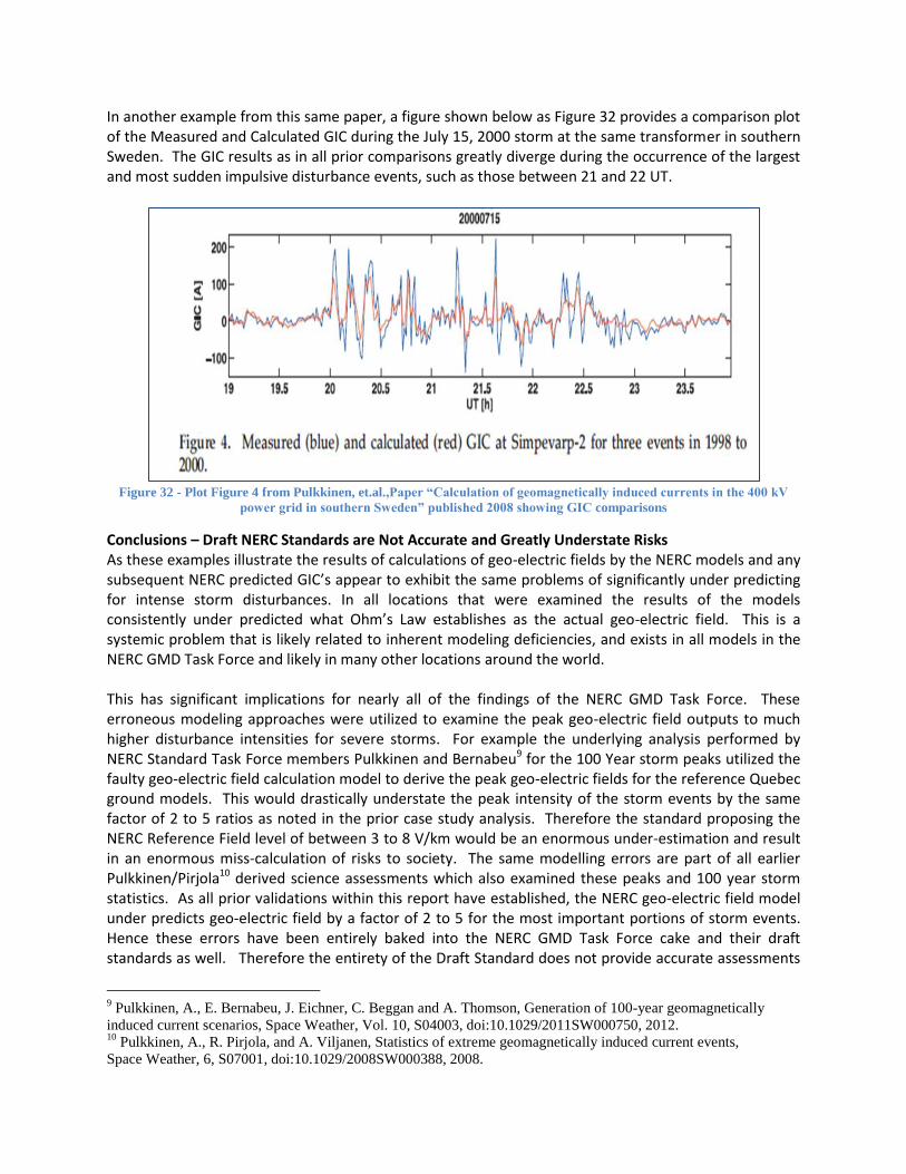
In another example from this same paper, a figure shown below as Figure 32 provides a comparison plot of the Measured and Calculated GIC during the July 15, 2000 storm at the same transformer in southern Sweden. The GIC results as in all prior comparisons greatly diverge during the occurrence of the largest and most sudden impulsive disturbance events, such as those between 21 and 22 UT.

Figure 32 - Plot Figure 4 from Pulkkinen, et.al.,Paper “Calculation of geomagnetically induced currents in the 400 kV

power grid in southern Sweden” published 2008 showing GIC comparisons

Conclusions – Draft NERC Standards are Not Accurate and Greatly Understate Risks As these examples illustrate the results of calculations of geo-electric fields by the NERC models and any subsequent NERC predicted GIC’s appear to exhibit the same problems of significantly under predicting for intense storm disturbances. In all locations that were examined the results of the models consistently under predicted what Ohm’s Law establishes as the actual geo-electric field. This is a systemic problem that is likely related to inherent modeling deficiencies, and exists in all models in the NERC GMD Task Force and likely in many other locations around the world. This has significant implications for nearly all of the findings of the NERC GMD Task Force. These erroneous modeling approaches were utilized to examine the peak geo-electric field outputs to much higher disturbance intensities for severe storms. For example the underlying analysis performed by NERC Standard Task Force members Pulkkinen and Bernabeu9 for the 100 Year storm peaks utilized the faulty geo-electric field calculation model to derive the peak geo-electric fields for the reference Quebec ground models. This would drastically understate the peak intensity of the storm events by the same factor of 2 to 5 ratios as noted in the prior case study analysis. Therefore the standard proposing the NERC Reference Field level of between 3 to 8 V/km would be an enormous under-estimation and result in an enormous miss-calculation of risks to society. The same modelling errors are part of all earlier Pulkkinen/Pirjola10 derived science assessments which also examined these peaks and 100 year storm statistics. As all prior validations within this report have established, the NERC geo-electric field model under predicts geo-electric field by a factor of 2 to 5 for the most important portions of storm events. Hence these errors have been entirely baked into the NERC GMD Task Force cake and their draft standards as well. Therefore the entirety of the Draft Standard does not provide accurate assessments

9 Pulkkinen, A., E. Bernabeu, J. Eichner, C. Beggan and A. Thomson, Generation of 100-year geomagnetically

induced current scenarios, Space Weather, Vol. 10, S04003, doi:10.1029/2011SW000750, 2012. 10

Pulkkinen, A., R. Pirjola, and A. Viljanen, Statistics of extreme geomagnetically induced current events,

Space Weather, 6, S07001, doi:10.1029/2008SW000388, 2008.

of the geo-electric field environments that will actually occur across the US. It has also been shown in this White Paper that undertaking a more rigorous development of validated geo-electric field standards can be done in a simple and efficient manner and that such data to drive these more rigorous findings already exists in many portions of the US. Efforts on the part of NERC’s standard team and the industry to withhold this material information are counter-productive to the overarching requirements to assure public safety against severe geomagnetic storm events. Such fundamental and significant flaws in technical calculations and procedural actions should not be a part of any proposed standard and a redraft must be undertaken.