examining small-scale geographic estimates from the american community survey 5-year data
DESCRIPTION
Examining Small-scale Geographic Estimates from the American Community Survey 5-year Data. Robert Kominski Thom File Social, Economic and Household Statistics Division (SEHSD) U.S. Census Bureau. Question:. • How good (or bad) are small-scale ACS data? - PowerPoint PPT PresentationTRANSCRIPT

Examining Small-scale Geographic Estimates from the American
Community Survey 5-year Data
Robert KominskiThom File
Social, Economic and Household Statistics Division (SEHSD)
U.S. Census Bureau

Question:• How good (or bad) are small-scale
ACS data?
• Uses 5-year data file (2005-2009)

Secondary Question:
How difficult (or easy) will it be to use the ACS data to actually answer research questions?

Approach
1. Identify a typical analytic “problem” that an applied researcher might encounter – and then try to answer it
2. Evaluate this process and the results

Evaluation
How do we determine quality of estimates?


Problem
High school dropouts in Washington, D.C.
• How bad is the problem?
• Is the problem geographically focused? • Can ACS data differentiate areas of the city?

Figure 1: D.C. Tract Map with Tract Identification Numbers
188 Census tracts in D.C.

Reminder• Important to evaluate from the perspective of a researcher NOT employed by the Census Bureau
• Must use publicly available data • Major focus on ease of use – we want to minimize any additional computations (“The mayor needs it NOW!”)
Data • PUMS option provides lots of analytical control, but not good for small geographies (PUMA=100k)
• Focus instead on ACS “pre-tabulated” data
- Tables in either AFF or data download- Data provided down to tract/block group

Figure 2: Example of Table B14005 for D.C. Tract 1
• Table provides estimate of 16-19 year olds, not enrolled and not HS grads, by gender
User must combine estimates and convert to a percentage, then re-compute standard error as a percentage

Several Analytic Possibilities:
- Persons 18-24 without a HS degree
- Persons 25+ with a HS degree
- Persons 18-24 with a HS degree
- Census 2000: Persons 25+ with a HS degree

Figure 3: Example of Table B15001 for D.C. Tract 1
• Table provides estimate of 18-24 year olds, not HS grads, by gender
User must combine estimates and convert to a percentage, then re-compute standard error as a percentage
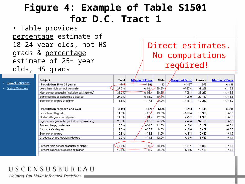
Figure 4: Example of Table S1501 for D.C. Tract 1
Direct estimates. No computations required!
• Table provides percentage estimate of 18-24 year olds, not HS grads & percentage estimate of 25+ year olds, HS grads
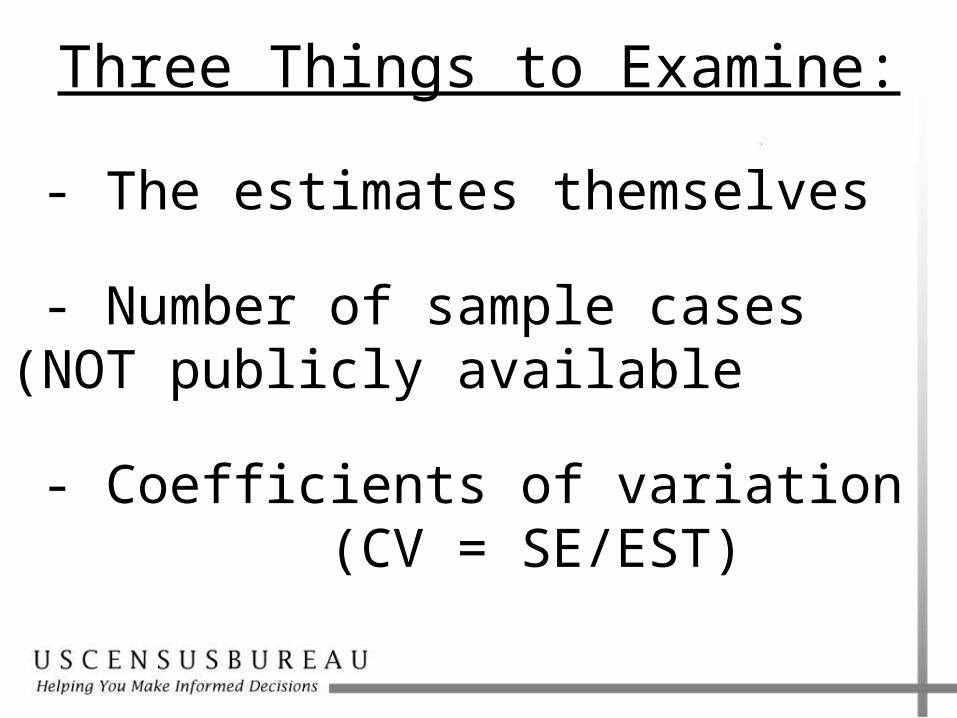
Three Things to Examine:
- The estimates themselves
- Number of sample cases (NOT publicly available
- Coefficients of variation (CV = SE/EST)

16
Estimates of High School Completion (or not)

Census 2000
18-24 Non HS Grads 18-24 HS Grads
ACS, ‘05-’09 ACS, ‘05-’09
Census 2000
25+ HS Grads
ACS, ‘05-’09
25+ HS Grads

18
Sample Data Counts

18-24 year olds25 years old +
All persons
ACS, ‘05-’09 ACS, ‘05-’09
Census 2000

20
Coefficients of Variation

18-24 Non HS Grads
18-24 HS Grads
25+ HS Grads 25+ HS Grads
ACS, ‘05-’09 ACS, ‘05-’09
ACS, ‘05-’09 Census 2000

- Smaller samples yield fewer cases of analytic interest
- Changing the sample increased the analytic sample (the numerator)
-Changing the universe also increased the analytic sample
-CV’s fall whenever S.E. drops or the estimate increases

How well do our measures correlate with one another?
• Measure 1 -- 2005-9 ACS Dropout level, ages 18-24
• Measure 2 -- 2005-9 ACS High school completion, ages 25+
• Measure 3 -- Census 2000 High school completion, ages 25+
• Measure 4 – 2005-9 ACS High school completion, ages 18-24
M1 M2 M3 M4
M1 * -.520 -.525 -1.00
M2 * .826 .520
M3 * .525
M4 *

• Small-scale geographic ACS data appear to be fairly robust
• Users will need to spend time thinking of the best way to approach their problem, but if they can find data that fit, small area geographic questions can be addressed
• Substantively, data are NOT misleading, particularly when considered in the proper context
Conclusions

25
Contact Information
U.S. Census BureauSocial, Economic and Household Statistics
Division
Robert [email protected]
Thom [email protected]