Example 5.1

Transportation Models

5.2 | 5.3 | 5.4 | 5.5 | 5.6 | 5.7 | 5.8 | 5.9 | 5.10 | 5.10a

Background Information

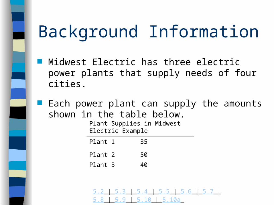
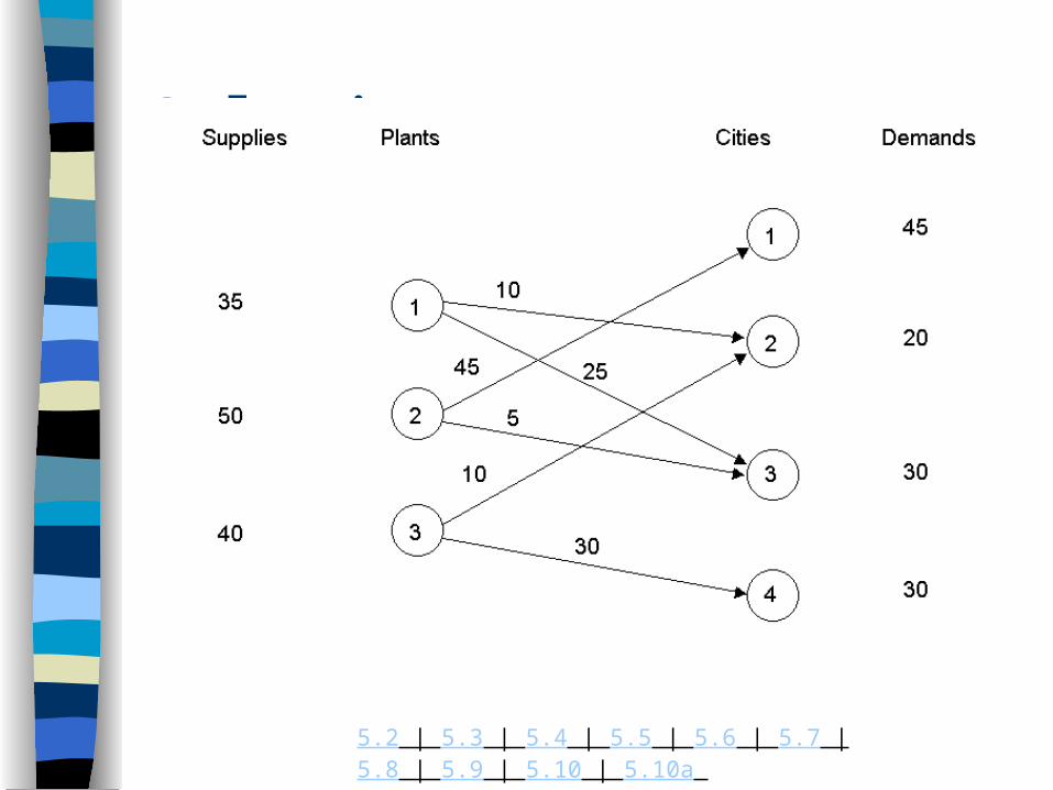
Midwest Electric has three electric power plants that supply needs of four cities.

Each power plant can supply the amounts shown in the table below.

Plant Supplies in Midwest Electric Example

Plant 1 35

Plant 2 50

Plant 3 40

5.2 | 5.3 | 5.4 | 5.5 | 5.6 | 5.7 | 5.8 | 5.9 | 5.10 | 5.10a

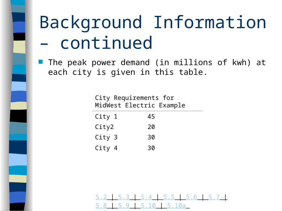
Background Information – continued The peak power demand (in millions of kwh) at each

city is given in this table.

City Requirements for MidWest Electric Example

City 1 45

City2 20

City 3 30

City 4 30

5.2 | 5.3 | 5.4 | 5.5 | 5.6 | 5.7 | 5.8 | 5.9 | 5.10 | 5.10a

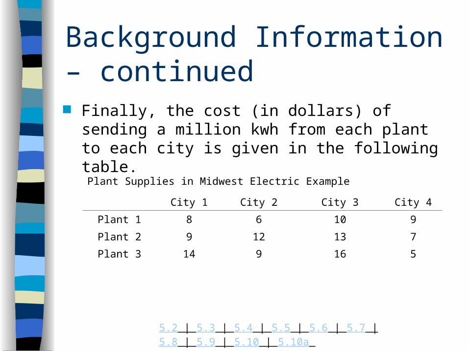
Background Information – continued Finally, the cost (in dollars) of sending a million kwh

from each plant to each city is given in the following table.

Plant Supplies in Midwest Electric Example

City 1 City 2 City 3 City 4

Plant 1 8 6 10 9

Plant 2 9 12 13 7

Plant 3 14 9 16 5

5.2 | 5.3 | 5.4 | 5.5 | 5.6 | 5.7 | 5.8 | 5.9 | 5.10 | 5.10a

Background Information – continued Midwest Electric wants to find the lowest cost method

for meeting the demand of the four cities.

5.2 | 5.3 | 5.4 | 5.5 | 5.6 | 5.7 | 5.8 | 5.9 | 5.10 | 5.10a

Solution

To set up a spreadsheet model for Midwest Electric’s problem, we need to keep track of the following:

– The power shipped (in millions of kwh) from each plant to each city

– The total power shipped out of each plant

– The total power received by each city

– The total shipping cost incurred.

5.2 | 5.3 | 5.4 | 5.5 | 5.6 | 5.7 | 5.8 | 5.9 | 5.10 | 5.10a

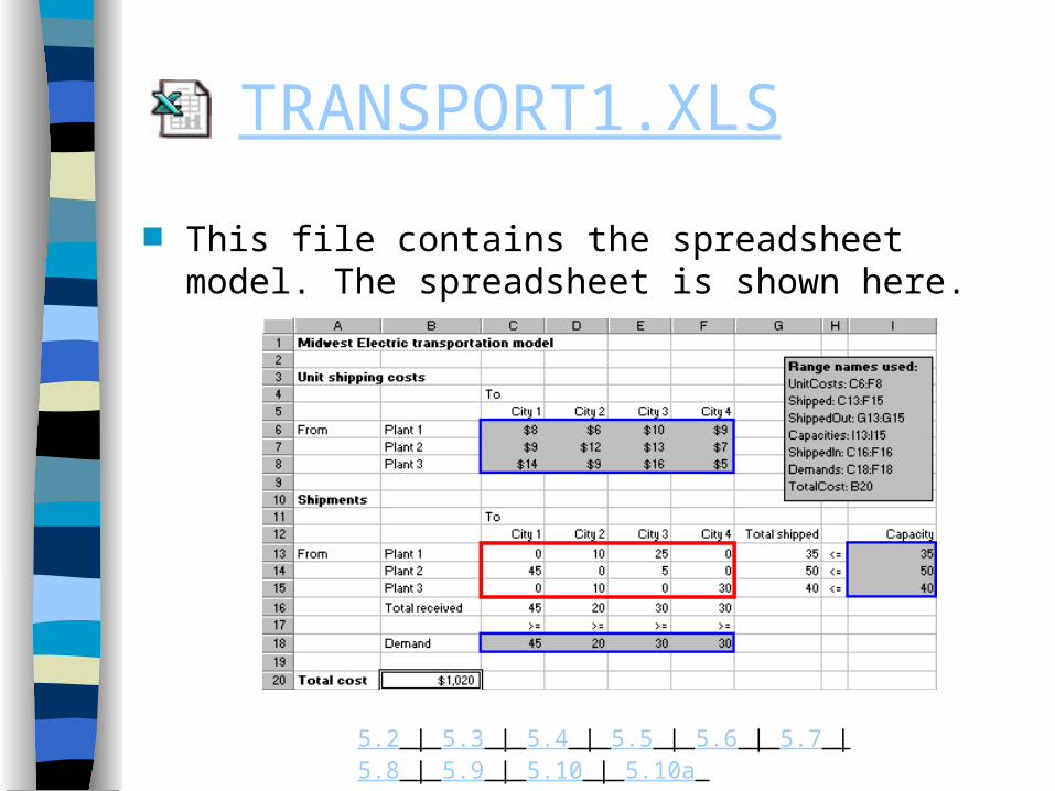
TRANSPORT1.XLS

This file contains the spreadsheet model. The spreadsheet is shown here.

5.2 | 5.3 | 5.4 | 5.5 | 5.6 | 5.7 | 5.8 | 5.9 | 5.10 | 5.10a

Developing the Model To develop this model, proceed as follows.

– Inputs. Enter the unit shipping costs for each plant to each city in the UnitsCosts range, the plant capacities in the Capacities, and the cities’ demands in the Demands range.

– Amounts shipped. Enter any trial values for the shipments from each plant to each city in the Shipped range. These are the changing cells.

– Amounts shipped out of plants. To ensure that a plant does not ship more than its available supply, we need to calculate the amount shipped out of each plant. In cell G13 calculate the amount shipped out of plant 1 with the formula =SUM(C13:F13) and copy this formula to the range G14:G15 for the other plants.

5.2 | 5.3 | 5.4 | 5.5 | 5.6 | 5.7 | 5.8 | 5.9 | 5.10 | 5.10a

Developing the Model – continued

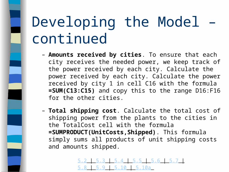
– Amounts received by cities. To ensure that each city receives the needed power, we keep track of the power received by each city. Calculate the power received by each city. Calculate the power received by city 1 in cell C16 with the formula =SUM(C13:C15) and copy this to the range D16:F16 for the other cities.

– Total shipping cost. Calculate the total cost of shipping power from the plants to the cities in the TotalCost cell with the formula =SUMPRODUCT(UnitCosts,Shipped). This formula simply sums all products of unit shipping costs and amounts shipped.

5.2 | 5.3 | 5.4 | 5.5 | 5.6 | 5.7 | 5.8 | 5.9 | 5.10 | 5.10a

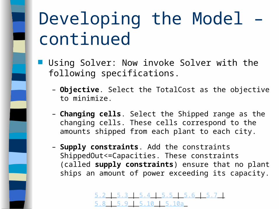
Developing the Model – continued Using Solver: Now invoke Solver with the following

specifications.

– Objective. Select the TotalCost as the objective to minimize.

– Changing cells. Select the Shipped range as the changing cells. These cells correspond to the amounts shipped from each plant to each city.

– Supply constraints. Add the constraints ShippedOut<=Capacities. These constraints (called supply constraints) ensure that no plant ships an amount of power exceeding its capacity.

5.2 | 5.3 | 5.4 | 5.5 | 5.6 | 5.7 | 5.8 | 5.9 | 5.10 | 5.10a

Developing the Model – continued

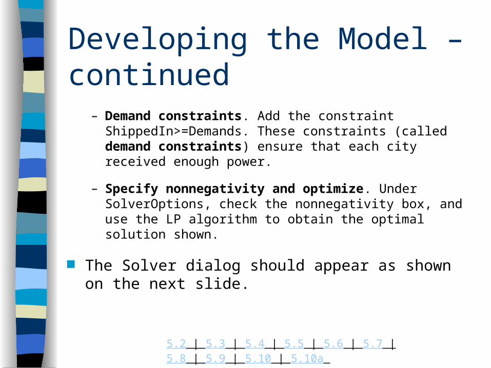
– Demand constraints. Add the constraint ShippedIn>=Demands. These constraints (called demand constraints) ensure that each city received enough power.

– Specify nonnegativity and optimize. Under SolverOptions, check the nonnegativity box, and use the LP algorithm to obtain the optimal solution shown.

The Solver dialog should appear as shown on the next slide.

5.2 | 5.3 | 5.4 | 5.5 | 5.6 | 5.7 | 5.8 | 5.9 | 5.10 | 5.10a

Developing the Model – continued

The Solver solution is illustrated graphically on the next slide.

5.2 | 5.3 | 5.4 | 5.5 | 5.6 | 5.7 | 5.8 | 5.9 | 5.10 | 5.10a

Solution

5.2 | 5.3 | 5.4 | 5.5 | 5.6 | 5.7 | 5.8 | 5.9 | 5.10 | 5.10a

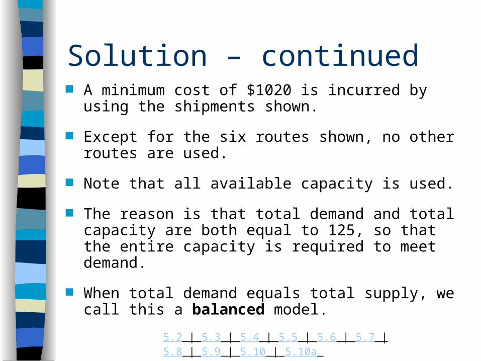
Solution – continued A minimum cost of $1020 is incurred by using the

shipments shown.

Except for the six routes shown, no other routes are used.

Note that all available capacity is used.

The reason is that total demand and total capacity are both equal to 125, so that the entire capacity is required to meet demand.

When total demand equals total supply, we call this a balanced model.

5.2 | 5.3 | 5.4 | 5.5 | 5.6 | 5.7 | 5.8 | 5.9 | 5.10 | 5.10a

Solution – continued If total capacity is greater than total demand, then

some of the capacity is less than total demand, we need to change the model, for in this case there is no way to meet total demand – Solver will report “no feasible solution.”

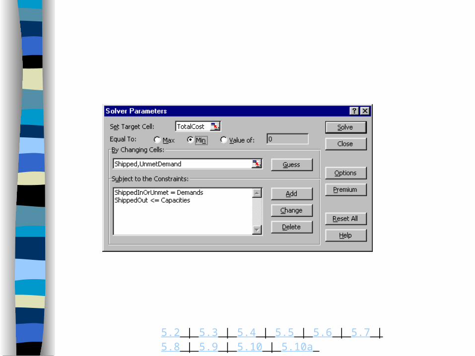
We need to drop the “greater than or equal to” demand constraints and probably include unit penalty costs for not meeting demand at the various cities.

A formulation along these lines appears in the Figure on the next slide, with the completed Solver dialog box shown on the slide after that.

5.2 | 5.3 | 5.4 | 5.5 | 5.6 | 5.7 | 5.8 | 5.9 | 5.10 | 5.10a

5.2 | 5.3 | 5.4 | 5.5 | 5.6 | 5.7 | 5.8 | 5.9 | 5.10 | 5.10a

5.2 | 5.3 | 5.4 | 5.5 | 5.6 | 5.7 | 5.8 | 5.9 | 5.10 | 5.10a

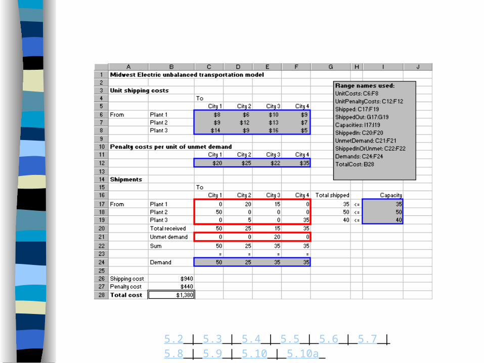
Solution – continued

Here we treat the unmet demand in row 21 as an extra set of changing cells, we add a constraint that requires the sums in row 22 to equal demand, and we account for the penalty cost of unmet demand in the total cost.

The optimal solution trades off shipping costs with the penalties from unmet demand.

In this case, the least-cost solution meets all demand except at city 3.

5.2 | 5.3 | 5.4 | 5.5 | 5.6 | 5.7 | 5.8 | 5.9 | 5.10 | 5.10a

Sensitivity Analysis

There are many sensitivity analyses we could perform on the basic transportation model.

We could vary one (or two) shipping costs, or we could vary capacities or demands.

One interesting analysis is to keep shipping costs and demands constant and allow all of the capacities to increase by a certain percentage.

This percentage becomes the input to SolverTable.

5.2 | 5.3 | 5.4 | 5.5 | 5.6 | 5.7 | 5.8 | 5.9 | 5.10 | 5.10a

Sensitivity Analysis – continued

Then we keep track of the total cost and any particular amounts shipped of interest.

The key is to modify the model slightly before running SolverTable.

The appropriate modifications appear in the model on the next slide.

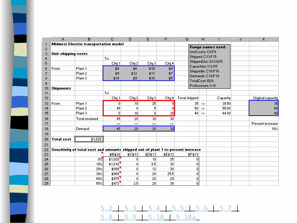
Now we store the original capacities in column K, we enter a percent increase in the PCtIncrease cell, and we enter formulas in the Capacities range.

5.2 | 5.3 | 5.4 | 5.5 | 5.6 | 5.7 | 5.8 | 5.9 | 5.10 | 5.10a

5.2 | 5.3 | 5.4 | 5.5 | 5.6 | 5.7 | 5.8 | 5.9 | 5.10 | 5.10a

Sensitivity Analysis – continued

Then we run the SolverTable with the PctIncrease cell as the single input cell, allowing it to vary from 0% to 50% in increments of 10%, and we keep track of total cost, as well as the shipments out of plant 1.

The results are possibly surprising. Because total demand is not changing, the extra capacity does not imply that we will ship more units total – there is no incentive to send more than the demands require.

However, the increased capacity gives us more flexibility to use lower-cost shipping routes.

5.2 | 5.3 | 5.4 | 5.5 | 5.6 | 5.7 | 5.8 | 5.9 | 5.10 | 5.10a

Sensitivity Analysis – continued

As we see, the total cost steadily decreases as more capacity is available, and we tend to take more advantage of the routes out of plant 1.

This sensitivity analysis demonstrates that even though transportation models are among the simplest of all LP models to formulate, their optimal solutions can have somewhat unintuitive properties.

5.2 | 5.3 | 5.4 | 5.5 | 5.6 | 5.7 | 5.8 | 5.9 | 5.10 | 5.10a

An Alternative Formulation

The transportation model is a very natural one. If we consider the graphical representation we note that all “flows” go from left to right, from suppliers to demanders.

Therefore, the rectangular range of shipments allows us to calculate shipments out of plants as row sums and shipments into cities as column sums.

In anticipation of later models in this chapter, however, where the graphical network can be more complex, we present an alternative formulation of the transportation model.

5.2 | 5.3 | 5.4 | 5.5 | 5.6 | 5.7 | 5.8 | 5.9 | 5.10 | 5.10a

TRANSPORT2.XLS

This file contains the model.

First, it is useful to introduce some standard network terminology.

When we represent a network model graphically, we generally connect circles with arrows.

The circles are called nodes. They generally represent cities, warehouses, manufacturing plants, or other locations.

5.2 | 5.3 | 5.4 | 5.5 | 5.6 | 5.7 | 5.8 | 5.9 | 5.10 | 5.10a

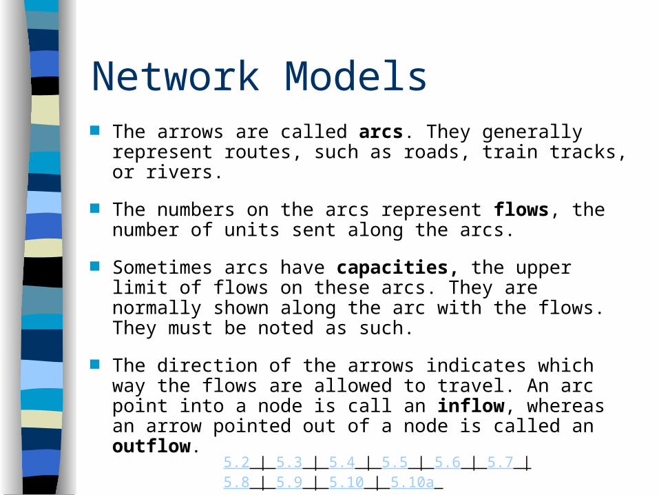
Network Models The arrows are called arcs. They generally represent

routes, such as roads, train tracks, or rivers.

The numbers on the arcs represent flows, the number of units sent along the arcs.

Sometimes arcs have capacities, the upper limit of flows on these arcs. They are normally shown along the arc with the flows. They must be noted as such.

The direction of the arrows indicates which way the flows are allowed to travel. An arc point into a node is call an inflow, whereas an arrow pointed out of a node is called an outflow.

5.2 | 5.3 | 5.4 | 5.5 | 5.6 | 5.7 | 5.8 | 5.9 | 5.10 | 5.10a

Network Models – continued

In the basic transportation model, all outflows originate from suppliers, and all inflows go toward demanders. However, general networks can have both inflows and outflows corresponding to any given node.

The typical network model has one changing cell per arc. It indicates how much to send along that arc.

Therefore it is often useful to model network problems by listing all of the arcs and their corresponding flows in one long list.

5.2 | 5.3 | 5.4 | 5.5 | 5.6 | 5.7 | 5.8 | 5.9 | 5.10 | 5.10a

Network Models – continued

Specifically, for each node in the network there will be a flow balance constraint. These flow balance constraints for the basic transportation model are simply the supply and demand constraints we have already discussed.

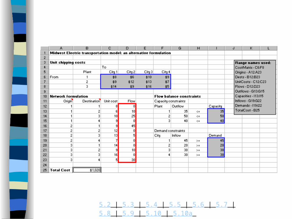
The alternative formulation of the Midwest Electric model appears on the next slide.

In the range A12:B23, we manually enter the plant and city indexes.

5.2 | 5.3 | 5.4 | 5.5 | 5.6 | 5.7 | 5.8 | 5.9 | 5.10 | 5.10a

5.2 | 5.3 | 5.4 | 5.5 | 5.6 | 5.7 | 5.8 | 5.9 | 5.10 | 5.10a

An Alternative Formulation – continued Each of these corresponds to a given name – that is

an arc is the network.

In column C we enter the unit shipping costs.

If they have already been entered in a rectangular range, as in the CostMatrix range, we can easily “transfer” them to the appropriate cells in the UnitCosts range by entering the formula =INDEX(CostMatrix,A12,B12 in cell C12 and copying it down.

5.2 | 5.3 | 5.4 | 5.5 | 5.6 | 5.7 | 5.8 | 5.9 | 5.10 | 5.10a

An Alternative Formulation – continued Then we enter a column of changing cells for the

flows in column D.

The flow balance constraints are conceptually straightforward.

Each cell in the Outflows and Inflows ranges contains the appropriate sum of changing cells.

Is there an easy way to take advantage of copying when entering these formulas?

5.2 | 5.3 | 5.4 | 5.5 | 5.6 | 5.7 | 5.8 | 5.9 | 5.10 | 5.10a

An Alternative Formulation – continued Fortunately, the answer is “yes”. We use Excel’s built

in SUMIF function, in the form =SUMIF(Range,Criteria,SumRange).

For example, the formula in cell G13 is =SUMIF(Origins,F13,Flows). This compares the plant number in cell F13 to the Options range in column A and sums all flows where they are equal – that is, it sums all flows out of plant 1.

By copying this down, we obtain the flows out of the other plants.

5.2 | 5.3 | 5.4 | 5.5 | 5.6 | 5.7 | 5.8 | 5.9 | 5.10 | 5.10a

An Alternative Formulation – continued For flows into cities, we enter the similar formula

=SUMIF(Dests,F19,Flows) in cell G19 to sum all flows into city 1, and we copy it down for flows into the other cities.

In general, the SUMIF function finds all cells in the first argument that satisfy the criteria in the second argument and then sums the corresponding cells in the third argument – a very hand function.

This use of the SUMIF function, along with the list of origins, destinations, unit costs, and flows in columns A-D, is the key to the network formulation.

5.2 | 5.3 | 5.4 | 5.5 | 5.6 | 5.7 | 5.8 | 5.9 | 5.10 | 5.10a

An Alternative Formulation – continued From there on, the model is straightforward.

We calculate the total cost as the SUMPRODUCT of UnitCosts and Flows, and we set up the Solver dialog box exactly as before.

To a certain extent this makes all network models alike.

There is an additional benefit from this model formulation.

5.2 | 5.3 | 5.4 | 5.5 | 5.6 | 5.7 | 5.8 | 5.9 | 5.10 | 5.10a

An Alternative Formulation – continued Suppose that, for whatever reason, flows from certain

plants to certain cities are not allowed.

It is easy to disallow such routes in the original formulation. The usual trick then is to allow the “disallowed” routes but impose extremely large unit shipping costs on them.

This works, but it is wasteful because it adds changing cells that do not really belong in the model. However, the current formulation simply omits arcs that are not allowed.

5.2 | 5.3 | 5.4 | 5.5 | 5.6 | 5.7 | 5.8 | 5.9 | 5.10 | 5.10a

An Alternative Formulation – continued This creates a model with exactly as many changing

cells as allowable arcs.

This additional benefit can be very valuable when the number of potential arcs in the network is huge, even though the vast majority of them are disallowed – and this is exactly the situation in most large network models.