example: explore the relationships among month, adv.$...

1

Simple and Multiple Regression Analysis

Example: Explore the relationships among Month, Adv.$ and Sales $:

1. Prepare a scatter plot of these data. The scatter plots for Adv.$ versus Sales, and Month versus

Sales are given in the Figures below with Excel@ Insert/Scatter.

a. Do the data appear to be stationary or nonstationary? The data appear to be

nonstationary, it is not random, but with clear linear trend upward.

b. Do the data appear to have a trend? Yes, the data have clear up trend, that is as the

Adv.$ or Month increase, the Sales increase as well.

c. If we want to fit a straight line to the data, how many lines could we possibly fit? We can

fit infinite number of straight lines to the data. Each line is represented with a different

set of b0 (Y intercept), b1 (Slope for Month) and b2 (Slope for Adv.$) for this case.

d. Compute the coefficient of correlation r between Month, Adv.$ and Sales, respectively,

with =CORREL(Array1,Array2) and interpret the meanings. r(Adv versus Sales) = 0.901

and r(Month versus Sales) = 0.9722 indicate strong positive correlation between the Adv

and Sales, and Month and Sales, respectably.

(Regression.xls/Reg0)

2. What is the general linear model to be used to model linear trend? (Write out the model)

�� = �� + �� + �� + � or � �� = �� + ��ℎ� + �� + �

2

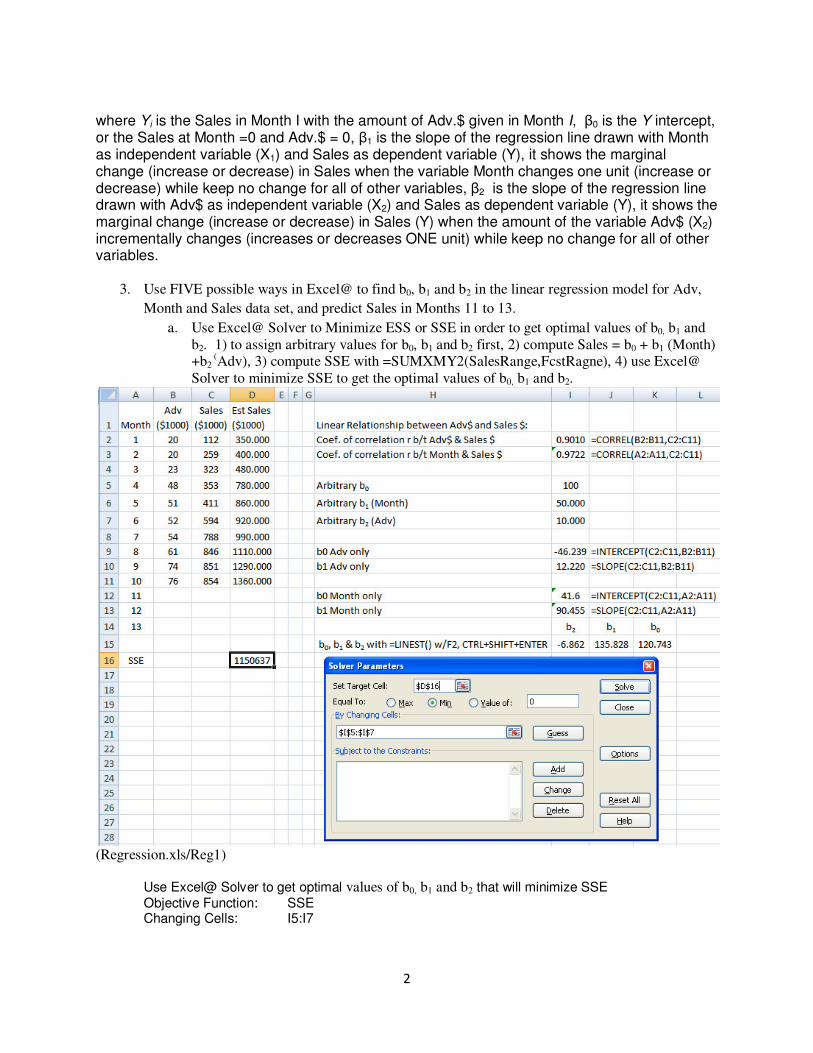
where Yi is the Sales in Month I with the amount of Adv.$ given in Month I, β0 is the Y intercept, or the Sales at Month =0 and Adv.$ = 0, β1 is the slope of the regression line drawn with Month as independent variable (X1) and Sales as dependent variable (Y), it shows the marginal change (increase or decrease) in Sales when the variable Month changes one unit (increase or decrease) while keep no change for all of other variables, β2 is the slope of the regression line drawn with Adv$ as independent variable (X2) and Sales as dependent variable (Y), it shows the marginal change (increase or decrease) in Sales (Y) when the amount of the variable Adv$ (X2) incrementally changes (increases or decreases ONE unit) while keep no change for all of other variables.

3. Use FIVE possible ways in Excel@ to find b0, b1 and b2 in the linear regression model for Adv,

Month and Sales data set, and predict Sales in Months 11 to 13.

a. Use Excel@ Solver to Minimize ESS or SSE in order to get optimal values of b0, b1 and b2. 1) to assign arbitrary values for b0, b1 and b2 first, 2) compute Sales = b0 + b1 (Month) +b2

(Adv), 3) compute SSE with =SUMXMY2(SalesRange,FcstRagne), 4) use Excel@ Solver to minimize SSE to get the optimal values of b0, b1 and b2.


Use Excel@ Solver to get optimal values of b0, b1 and b2 that will minimize SSE Objective Function: SSE Changing Cells: I5:I7

3

b. Use Excel@ Data/Data Analysis/Regression to get the Summary Output for the data and print a copy of it, find values of b0, b1, and b2 in the Summary Output. The values of b0, b1, and b2 are labeled in the Summary Output below.

(Regression.xls/Reg1SOa)

c. Use Excel@ =LINEST(ArrayY, ArrayXs) to get b0, b1 and b2 simultaneously. Use

Excel@ =LINEST(C2:C11,A2:B11) as in Regression.xls/Reg1. Note, Highlight the I15:K15, type =LINEST(C2:C11,A2:B11), then CTRL+SHIFT+ENTER.


d. =INTERCEPT(Y-RANGE,X-RANGE) for b0 and =SLOPE(Y-RANGE,X-RANGE) for b1 when only single X variable is considered each time.


4

e. Click any data point on the scatter plots for Month and Sales, or Adv and Sales, select Add Trendline / Display equations & Display R-Squared value on the charts. The Y and Xs are renamed to Month, Adv and Sales, respectively, for the regression lines.

4. What are the values of b0, b1, and b2, and what is the estimated regression function? The values

of b0, b1, and b2 are 120.7428, 135.8275 and -6.862, respectively as given in the Table above.

5. What are the meaning of b0, b1, and b2? When in Month=0, and Adv=0, the Sales =

b0=$120.7428, b1=$135.8275 shows the marginal change (increase or decrease) of

$135.8275 in Sales when the variable Month changes one unit (increase or decrease)

while keep no change for Adv., b2 = –6.862 shows the marginal change (decrease or

increase) of –$6.862 in Sales (Y) when the amount of the variable Adv$ (X2)

incrementally changes (increases or decreases ONE unit) while keep no change for

Month.

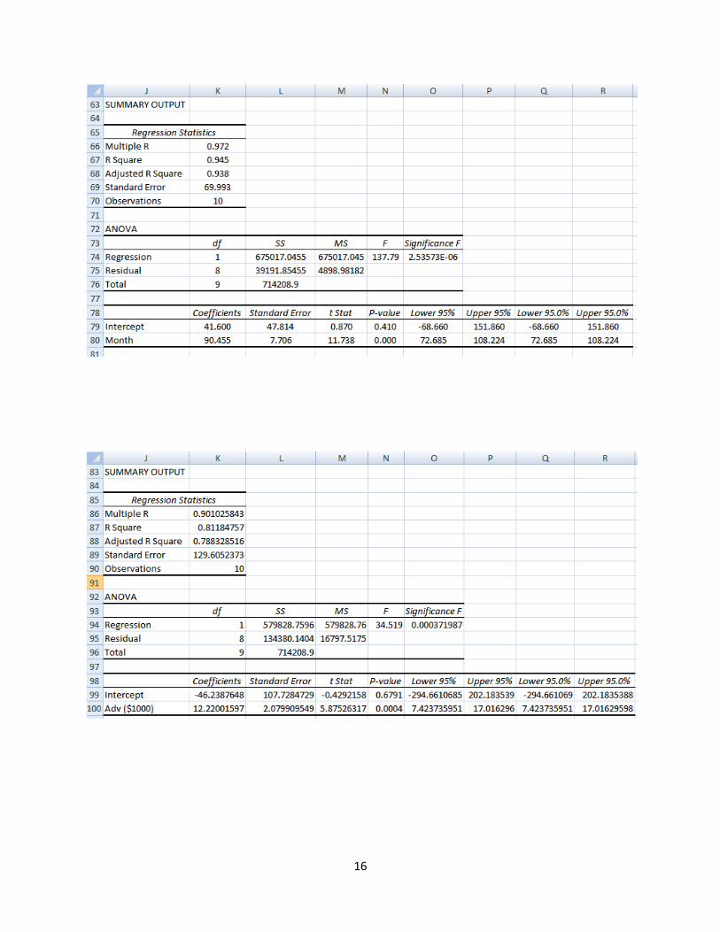
6. Use Excel@ =RSQ(Array Y,Array X) to compute the coefficient of Determination R2 of the regression line for the data, and interpret the meaning of R2 for the data?

(Regression.xls/Reg1) For the regression line for Month versus Sales, R2 = 94.5% means 94.5% of the total variations in Sales are counted for or explained and 5.5% of the total variations are not counted for or not explained by the regression line between Month and Sales. For the regression line for Adv versus Sales, R2 = 81.18% means 81.18% of the total variations in Sales are counted for or explained and 18.82%% of the total variations are not counted for or not explained by the regression line between the Adv and Sales.

7. For the Summary Table from Data/Data Analysis, answer the following questions: a. R2, Adjusted R2, Number of Observations, b0, b1, p-value for b0, p-value for b1. The

values are as labeled in the above table from Regression.xls/Reg1SO. b. Use the p-value approach to test the population parameters β0, β1 and β2 with the p-values

from the Summary Output of Data Analysis/Regression, and state your conclusion. Assume the significance coefficient α = 0.05.

(Regression.xls/Reg1SOa)

Hypothesis Test for β0: i. What are the H0 and H1? H0: β0 = 0 and H1: β0 ≠0

ii. What are the decision rules? Decision Rules with p-value Approach: If p-value ≥ α (significance coefficient), then conclude H0 or β0 = 0; Otherwise, if p-value < α, then conclude Ha, or β0 ≠0.

iii. What is the conclusion? The p-value for β0 = 0.082 as given in the Summary Output, it is greater than α = 0.05, therefore, we conclude H0: β0 = 0 or fail to reject H0, i.e., we should not include the Y intercept term in the regression model for Sales.

5

Hypothesis Test for β1(Month):

i. What are the H0 and H1? H0: β1 = 0 and H1: β1 ≠0 ii. What are the decision rules?

Decision Rules with p-value Approach: If p-value ≥ α (significance coefficient), then conclude H0 or β1 = 0; Otherwise, if p-value < α, then conclude Ha, or β1 ≠0.

iii. What is the conclusion? The p-value for β1 = 0.001 as given in the Summary Output, it is less than α = 0.05, therefore, we conclude H1: β1 ≠0 or reject reject H0, i.e., we should include the variable Month in the regression model for Sales.

Hypothesis Test for β2(Adv):

i. What are the H0 and H1? H0: β2 = 0 and H1: β2 ≠0 ii. What are the decision rules?

Decision Rules with p-value Approach: If p-value ≥ α (significance coefficient), then conclude H0 or β2 = 0; Otherwise, if p-value < α, then conclude Ha, or β2 ≠0.

iii. What is the conclusion? The p-value for β2 = 0.105 as given in the Summary Output, it is greater than α = 0.05, therefore, we conclude H0: β0 = 0 or fail to reject H0, i.e., we should not include the variable Adv in the regression model for Sales.

Therefore the final regression model for Sales becomes: Sales = b1 (Month). We have to go through additional procedures below to find out the value of b1 when the Y intercept b0 is zero. For reference: Decision Rules with Confidence Interval Approach: If the given CI spans zero (with zero as part of CI), conclude H0 Otherwise, if the given CI does not span zero, then conclude Ha

8. What are the forecasts for the next two years (11 to 12) with the regression line? Because the

hypothesis tests reveal only β1 is significant and should be included in the model, we further run

the models with Adv only and Month only with the results in the following two tables.

(Regression.xls/Reg1SOb)

(Regression.xls/Reg1SOc)

6

The results reveal that the Y intercept terms on both cases are not significant, thus should not be

included in the model, the variables Month and Adv, each is significant to model the Sales by

itself. We therefore decide to use Month only as recommended in the procedure 7.b above. To

find out the value of b1 without b0 with the variable Month only, we need to rerun the Data/Data

Analysis/Regression with the option of Constant is Zero as given below.


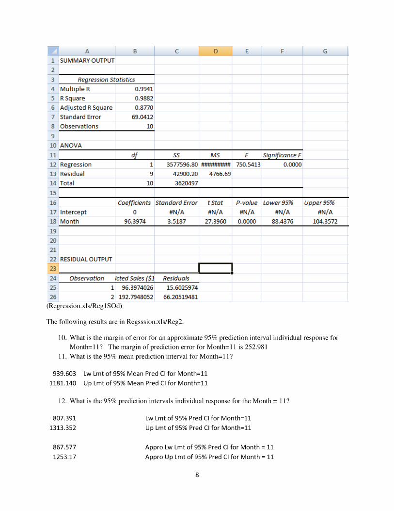
The final Summary Output Table is given in Regression.xls/Reg1SOd)

(Regression.xls/Reg1SOd)

a. Manually compute the forecasts with the b0 ,b1 and b2 from the previous results

Sales (Month=11) = 96.3974 * 11 (Month) = $1060.37 in Excel@ =Reg1SOd!$B$18*'Reg1'!A12

Sales (Month=12) = 96.3974 * 12 (Month) = $1156.77 in Excel@ =Reg1SOd!$B$18*'Reg1'!A13

In this case, Excel@ = TREND() cannot be used to forecast future Sales. The following

procedures are used to show how to use =TREND() to forecast Sales when b0, b1, and b2 are all

included in the model for Sales. We use TREND2 to represent the forecasts developed with

=TREND() with both Month and Adv in the model for Sales. Assume the Adv = 35 for Month =

11, and Adv = 45 for Month = 12. Please note the use of Absolute Address in =TREND().

7

b. Use Excel@ =TREND(Y-RANGE,X-RANGE,X-VALUE)


c. What is the assumption you made when you develop forecasts for the next two years?

The crucial assumption made for using linear regression is that the linear trend for Sales

is going to continue in Months 11 and 12 with the b2 = 96.3974. Thus any forecasts made

outside out the original ranges of independent variable Xs in the historical data may not

be valid.

9. What is the difference between standard error (Se) and the standard prediction error (Sp)?

Standard Error of Estimate (�� Se):

�� = �� = �∑ (�� − �!�)#�$�� − % − 1 = � ��'� − % − 1 = √��' = )��' = 69.0412

Se measures the variation of the actual data around the estimated regression line, where k is the

number of independent variables in the model.

Standard prediction error (Sp): thus the Sp is always larger than Se.

�0 = ��1 + 1� + (��1 − �2)∑ (��1 − �2)#�$�

(1–α)% Prediction Interval for individual response Y:

�!�1 = 3� + 3��1 and �!�1 ± �(�567;#5)�0

8

(Regression.xls/Reg1SOd)

The following results are in Regsssion.xls/Reg2.

10. What is the margin of error for an approximate 95% prediction interval individual response for

Month=11? The margin of prediction error for Month=11 is 252.981

11. What is the 95% mean prediction interval for Month=11?

939.603 Lw Lmt of 95% Mean Pred CI for Month=11

1181.140 Up Lmt of 95% Mean Pred CI for Month=11

12. What is the 95% prediction intervals individual response for the Month = 11?

807.391

Lw Lmt of 95% Pred CI for Month=11

1313.352

Up Lmt of 95% Pred CI for Month=11

867.577

Appro Lw Lmt of 95% Pred CI for Month = 11

1253.17

Appro Up Lmt of 95% Pred CI for Month = 11

9


10

Topics to be covered:

1. Regression as a method in business analytics � = 9(��, �, ; , �<) + a. Simple Linear Regression (SLP)

� = 9(�) + or �� = �� + �� + � and 3� and 3�as estimates for ��, �� !� = 3� + 3�� to min '�� = ∑ (#�$� �� − �!�) = ∑ =#�$� �� − (3� + 3��)> and the method of least squares

b. Simple Linear Regression with Time as Independent Variable � = 9(?) + @ or �� = �� + ��?� + � c. Multiple Regression � = 9(��, �, ; , �<) + , where f(.) describes systematic

variations and ε describers unsystematic variations of the system.

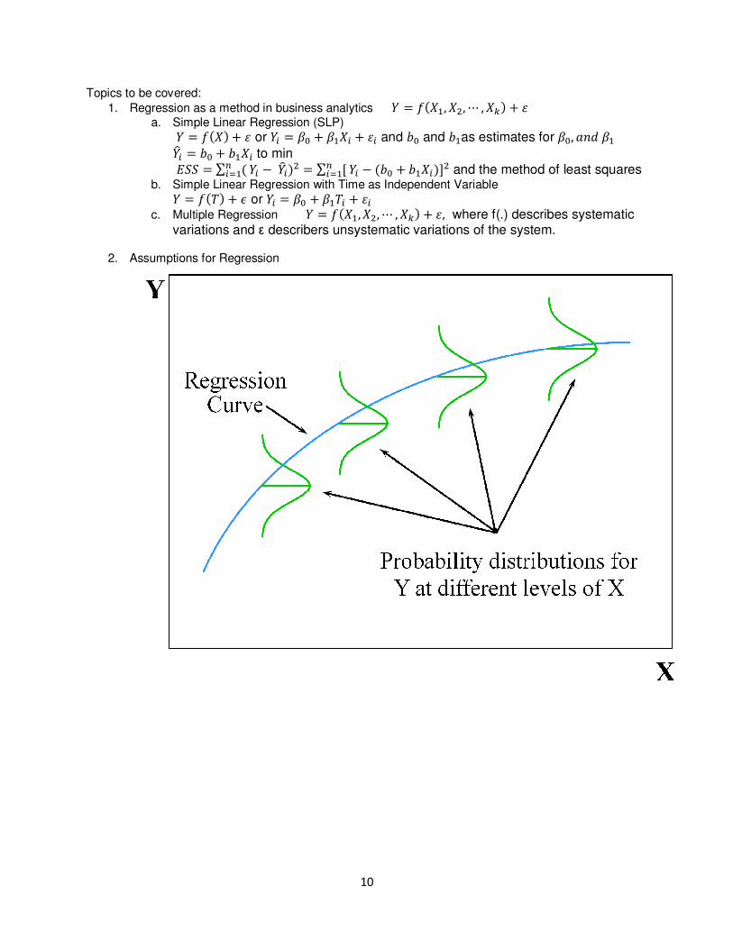
2. Assumptions for Regression

11

3. Using Excel@ to do Regression analysis

�! = 3� + 3�� 2 • �� − �2 �� − �!� �!� �!� − �2

Decomposition of the Total Error: �� − �2 = (�� − �!�) + (�!� − �2)

A(�� − �2)#�$�

= A(��#

�$�− �!�) + A(�!�

#�$�

− �2)

TSS = ESS + RSS

Or Total Sum of Squared Errors (TSS) = Error Sum of Squares (ESS) + Regression Sum of Squares (RSS)

) = BCCDCC = 1 − ECCDCC, and 0 ≤ R2 ≤ 1

R2 refers to the percentage of the total variation of Y around its mean that is explained or counted for by

the estimated regression line or how well the regression line fits the data.

1-R2 is the percentage of the total variation of Y around its mean that is unexplained or uncounted for by

the regression line.

Equations to compute b0 and b1:

3� = �� = ∑ (�� − �2)(�� − �2)#�$�∑ (�� − �2)#�$� = ∑ �� − =∑ ��#�$� >=∑ ��#�$� >�#�$�∑ ��#�$� − F∑ ��#�$� G

�

3� = �2 − 3��2

12

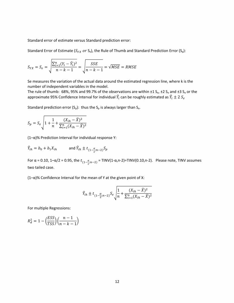
Standard error of estimate versus Standard prediction error:

Standard Error of Estimate (�� Se), the Rule of Thumb and Standard Prediction Error (Sp):

�� = �� = �∑ (�� − �!�)#�$�� − % − 1 = � ��'� − % − 1 = √��' = )��'

Se measures the variation of the actual data around the estimated regression line, where k is the

number of independent variables in the model.

The rule of thumb: 68%, 95% and 99.7% of the observations are within ±1 Se, ±2 Se and ±3 Se or the

approximate 95% Confidence Interval for individual �!� can be roughly estimated as �!� ± 2 ��

Standard prediction error (Sp): thus the Sp is always larger than Se.

�0 = ��1 + 1� + (��1 − �2)∑ (��1 − �2)#�$�

(1–α)% Prediction Interval for individual response Y:

�!�1 = 3� + 3��1 and �!�1 ± �(�567;#5)�0

For α = 0.10, 1–α/2 = 0.95, the �(�567;#5) = TINV(1-α,n-2)=TINV(0.10,n-2). Please note, TINV assumes

two tailed case.

(1–α)% Confidence Interval for the mean of Y at the given point of X:

�!�1 ± �(�5H;#5)��1� + (��1 − �2)∑ (��1 − �2)#�$�

For multiple Regressions:

)I = 1 − J'��?��K J � − 1� − % − 1K

13

Statistical Tests for β0, β1, ;, βk with F-Statistic, p-value and t-statistic:

• How to get the regression line in Excel@?

o =INTERCEPT(Y-RANGE,X-RANGE) and =SLOPE(Y-RANGE,X-RANGE)

o =TREND(Y-RANGE,X-RANGE,X-VALUE)

o In Excel@ Data/Data Analysis/Regression

o In Excel@, insert/scatter plot, Click any data points in the scatter plot, select Add

Trendline / Display equations & Display R-Squared value on chart

o Use Excel Solver to Minimize ESS

What are the meanings of the slope(β1, … βn) and the intercept(β0)? Meanings of b0 and b1:

o b0 is the intercept or Y value as X = 0 (e.g. Fixed cost)

o b1 is the slope or marginal change in Y with unit change in X

o b1 is similar to the slope. However, since it is calculated with the variability of the data

in mind, its formulation is not as straight-forward as our usual notion of slope.

• How to statistically test whither β0, β1, … βn equals zero (in the Null Hypothesis H0)?

o Use the p-value approach because p-values will be in Summary Output. Decision Rule is:

if p-value is less than α value (Type I error, not the one in Exponential smoothing

forecasting), then conclude β0, β1, … βn not equal to zero.

o Only include b0, b1, …, bn in the equation if β0, β1, … βn not equal to zero. Exclude the

zero ones

• How to interpret R2? Percentage of total variations explained by the regression line. (1-R2) is

the percentage of total variations not explained by the regression line.

• How to develop forecasts with given b0, b1, …, bn?

o �!�1 = 3� + 3��1 + 3��L for each value of X and could be X1, X2, …, and Xn.

14

o Predictions made using an estimated regression function may have little or no validity

for values of the independent variables that are substantially different from those

represented in the sample.

o Avoid multicollinearity when more than one independent variables are in the model.

• How to estimate the prediction confidence intervals?

o The approximate prediction confidence interval, �!� ± 2 ��, where Se is the standard

error given in the Summary Output beneath the Adjusted R2.

o The prediction confidence interval for the mean response is given by �!� ± � ��M��

o The prediction confidence interval for individual response is given by �!� ± � �0, where Sp

is the standard prediction error and Sp is always larger than Se.

• How to develop forecasting with Trend, Seasonal and Random components with the

multiplicative model Y = T.S.I?

o Use regression or centered moving average to take out the trend component – deTrend

o Use S.I = Y/T to get the percentage of Trend

o Compute Seasonal Relatives by average the percentages of Trend in the same season

o Adjust the Seasonal Relatives to the whole number (Quarterly seasonality in a year will

be 4, Weekly seasonality will be 7, etc.) to get the Seasonal Index.

o Attached the Seasonal Index to each season

o Develop the trend forecast with regression or other methods

o Use the Seasonal Index to multiply the previous forecasts to develop the final seasonally

adjusted forecast.

15

Simple Linear Regression with Time as Independent Variable

� = 9(?) + @ or �� = �� + ��?� + � and �!� = 3� + 3��

y = 12.22x - 46.239

R² = 0.8118

0

100

200

300

400

500

600

700

800

900

1000

0 10 20 30 40 50 60 70 80

Adv ($1000)

Sales ($1000)

y = 90.455x + 41.6

R² = 0.94510

200

400

600

800

1000

0 2 4 6 8 10 12

Month

Sales ($1000)

17

•

18

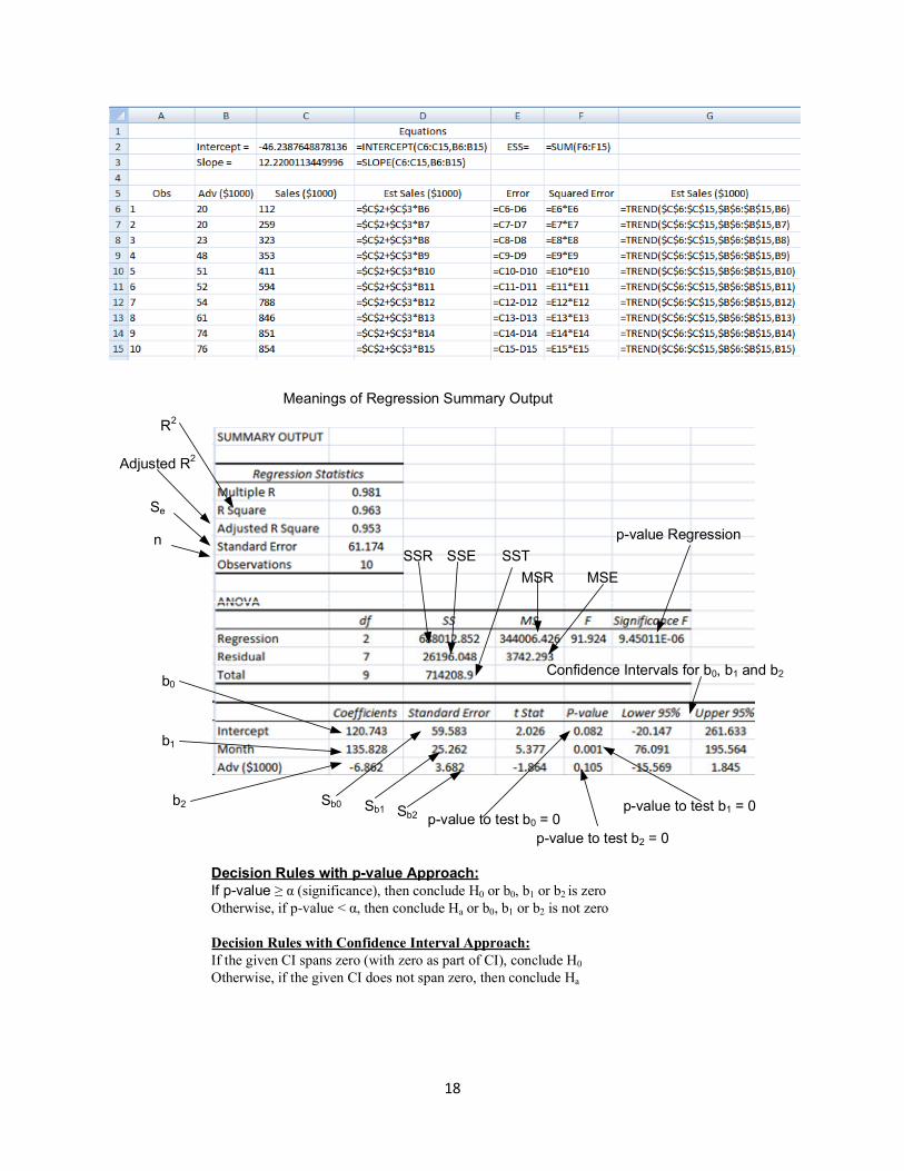
Meanings of Regression Summary Output

R2

Adjusted R2

Se

n

b0

b1

b2 Sb0 Sb1 Sb2

SSTSSR SSE

MSR MSE

p-value Regression

p-value to test b0 = 0p-value to test b1 = 0

p-value to test b2 = 0

Confidence Intervals for b0, b1 and b2

Decision Rules with p-value Approach:

If p-value ≥ α (significance), then conclude H0 or b0, b1 or b2 is zero

Otherwise, if p-value < α, then conclude Ha or b0, b1 or b2 is not zero

Decision Rules with Confidence Interval Approach:

If the given CI spans zero (with zero as part of CI), conclude H0

Otherwise, if the given CI does not span zero, then conclude Ha

example: explore the relationships among month, adv.$...

Documents