excel 2002 (xp) - utsc.utoronto.cawainbantin/a01s08/lectures/excel... · excel 2002 - lvl 2 lesson...
TRANSCRIPT

EXCEL 2002 (XP)
LEVEL 2: INTERMEDIATE FEATURES December 19, 2005


Organizational & Staff Development, U of T Page i
ABOUT GLOBAL KNOWLEDGE, INC. Global Knowledge, Inc., the world’s largest independent provider of integrated IT education solutions, is dedicated to improving the way companies and individuals learn, use, and master technology. The company’s educational solutions empower customers with choice, allowing them to determine when, where, and how they want their IT education programs to be designed and delivered. Global Knowledge’s blended IT education solutions combine vendor-authorized content with Global Knowledge developed curricula and deliver this through the right mix of intensive hands-on classroom training and interactive e-learning. Global Knowledge has a large, growing portfolio of e-learning content, products, and services. For large businesses, the company offers complete program management including enrollment, assessment, progress tracking and certification.
COPYRIGHT & TRADEMARKS © Copyright 2002 Global Knowledge Network, Inc. All rights reserved. No part of this publication, including interior design, cover design, icons or content may be reproduced by any means, be it transmitted, transcribed, photocopied, stored in a retrieval system, or translated into any language in any form, without the prior written permission of Global Knowledge Network, Inc. (“Global Knowledge”). Trademarks: All brand names used in this book are trade names, service marks, trademarks, or registered trademarks of their respective owners. CustomDOC® is a registered trademark of Global Knowledge, Inc. Courseware Express™, Global Knowledge™, and the Global Knowledge logo are trademarks of Global Knowledge.
DISCLAIMERS LIMIT OF LIABILITY/DISCLAIMER OF WARRANTY: Author and publisher have used their best efforts in preparing this book. Global Knowledge makes no representations or warranties with respect to the accuracy or completeness of the contents of this book and specifically disclaims any implied warranties of merchantability or fitness for a particular purpose. There are no warranties that extend beyond the descriptions contained within this paragraph. No warranty may be created or extended by any sales representative or sales materials. The accuracy and completeness of the information contained herein and the opinions stated herein are not guaranteed or warranted to produce any particular results, and the advice and strategies contained herein may not be suitable for every individual. Global Knowledge, Inc. shall not be liable for any loss of profit or any other commercial damages, including but not limited to special, incidental, consequential, or other damages.
Published By: Global Knowledge Network, Inc.
Knowledge Products Division 475 Allendale Road, Suite 102
King of Prussia, PA 19406 1-610-337-8878
http://www.kp.globalknowledge.com

Page ii Organizational & Staff Development, U of T
LEVEL 2: INTERMEDIATE FEATURES
ABOUT GLOBAL KNOWLEDGE, INC................................................................. I
COPYRIGHT & TRADEMARKS............................................................................ I
DISCLAIMERS .......................................................................................................... I
LESSON 1 - USING LARGE WORKSHEETS ......................................................1 Increasing the Magnification ....................................................................................2 Decreasing the Magnification...................................................................................3 Changing the Magnification of a Range...................................................................4 Switching to Full Screen View.................................................................................5 Splitting the Window................................................................................................6 Removing Split Windows.........................................................................................8 Freezing the Panes....................................................................................................8 Unfreezing the Panes ................................................................................................9
LESSON 2 - WORKING WITH MULTIPLE WORKSHEETS.........................11 Using Multiple Worksheets ....................................................................................12 Navigating between Worksheets ............................................................................13 Selecting Worksheets .............................................................................................14 Renaming Worksheets............................................................................................15 Selecting Multiple Worksheets...............................................................................15 Coloring Worksheet Tabs.......................................................................................16 Inserting Worksheets ..............................................................................................17 Deleting Worksheets ..............................................................................................18 Printing Selected Worksheets.................................................................................18
LESSON 3 - MANAGING WORKSHEETS.........................................................20 Copying Worksheets ..............................................................................................21 Moving Worksheets................................................................................................22 Using Grouped Worksheets....................................................................................22 Moving Data between Worksheets.........................................................................23 Copying Data between Worksheets........................................................................24 Creating 3-D Formulas ...........................................................................................25 Using 3-D Ranges in Functions..............................................................................27

Organizational & Staff Development, U of T Page iii
LESSON 4 - USING PASTE OPTIONS................................................................29 Copying/Cutting and Pasting Data .........................................................................30 Using the Paste Options Button..............................................................................32 Using the Paste List ................................................................................................33 Using the Clipboard Task Pane ..............................................................................35
LESSON 5 - USING RANGE NAMES..................................................................38 Working with Range Names ..................................................................................39 Jumping to a Named Range....................................................................................39 Assigning Names....................................................................................................40 Using Range Names in Formulas ...........................................................................42 Creating Range Names from Headings ..................................................................43 Applying Range Names..........................................................................................45 Deleting Range Names ...........................................................................................46 Using Range Names in 3-D Formulas....................................................................47 Creating 3-D Range Names....................................................................................49 Using 3-D Range Names in Formulas....................................................................50
LESSON 6 - CREATING SIMPLE FORMULAS................................................52 Using Formulas ......................................................................................................53 Entering Formulas ..................................................................................................54 Using Functions......................................................................................................56 Entering Basic Functions........................................................................................56 Inserting Functions in Formulas .............................................................................58 Editing Functions ...................................................................................................60 Using the AutoCalculate Feature............................................................................61 Using Range Borders to Modify Formulas.............................................................62 Checking Errors......................................................................................................64
LESSON 7 - WORKING WITH LABELS IN FORMULAS...............................66 Using Labels in Formulas.......................................................................................67 Using Labels to Define a Range.............................................................................67 Using Multiple Stacked Headings ..........................................................................69 Referring to Individual Cells ..................................................................................70
LESSON 8 - CREATING AND EDITING CHARTS ..........................................72 Using Charts ...........................................................................................................73

Page iv Organizational & Staff Development, U of T
Creating Charts with the Chart Wizard ..................................................................74 Moving and Resizing Charts ..................................................................................75 Identifying Chart Objects .......................................................................................76 Changing the Chart Type........................................................................................78 Changing the Chart Type and Sub-type .................................................................79 Changing the Plot Direction ...................................................................................80 Removing/Adding a Legend...................................................................................81 Moving the Legend.................................................................................................82 Charting Non-adjacent Ranges...............................................................................83 Changing the Chart Range......................................................................................84 Changing the Data Source ......................................................................................85 Changing the Chart Location..................................................................................86 Printing a Chart.......................................................................................................86 Deleting a Chart......................................................................................................87
LESSON 9 - FORMATTING CHARTS................................................................88 Formatting Charts...................................................................................................89 Adding Chart Titles ................................................................................................89 Formatting Chart Objects .......................................................................................90 Changing the Text Orientation ...............................................................................91
LESSON 10 - DRAWING AN OBJECT................................................................93 Working with Drawing Objects..............................................................................94 Drawing Enclosed Objects .....................................................................................94 Drawing a Line .......................................................................................................95 Selecting Filled and Unfilled Objects.....................................................................96 Moving an Object ...................................................................................................97 Adding Text to an Object .......................................................................................98 Selecting Text in an Object ....................................................................................99 Resizing an Object................................................................................................100 Formatting Lines ..................................................................................................100 Changing and Removing the Fill Color................................................................102 Changing the Font Color ......................................................................................103 Deleting an Object ................................................................................................104
LESSON 11 - USING ADDITIONAL EFFECTS AND OBJECTS ..................105 Adding a 3-D Effect .............................................................................................106
Organizational & Staff Development, U of T Page v
Applying a 3-D Setting.........................................................................................107 Adding a Shadow .................................................................................................107 Drawing a Text Box .............................................................................................108 Drawing an Arrow................................................................................................110 Inserting Pictures ..................................................................................................110 Formatting Graphics.............................................................................................112
LESSON 12 - USING AUTOSHAPES AND DIAGRAMS................................114 Working with AutoShapes ...................................................................................115 Drawing a Callout.................................................................................................115 Drawing a Basic Shape.........................................................................................117 Drawing a Connector............................................................................................118 Drawing a Flowchart Shape .................................................................................119 Drawing a Block Arrow .......................................................................................120 Inserting a Diagram ..............................................................................................121 Working with Diagrams .......................................................................................122
LESSON 13 - WORKING WITH COMMENTS................................................125 Creating Comments ..............................................................................................126 Viewing a Comment.............................................................................................127 Using the Reviewing Toolbar...............................................................................127 Printing Comments...............................................................................................129 Responding to Discussion Comments ..................................................................130
INDEX......................................................................................................................132


LESSON 1 - USING LARGE WORKSHEETS
In this lesson, you will learn how to:
• Increase the magnification
• Decrease the magnification
• Change the magnification of a range
• Switch to Full Screen view
• Split the window
• Remove split windows
• Freeze the panes
• Unfreeze the panes

Lesson 1 - Using Large Worksheets Excel 2002 - Lvl 2
Page 2 Organizational & Staff Development, U of T
INCREASING THE MAGNIFICATION
Discussion You can increase the magnification of the worksheet. Magnifying a worksheet is similar to using a magnifying glass; it makes the cells and their contents appear larger. This option is useful when you want to view a small portion of the worksheet in greater detail. For example, with a worksheet containing annual sales, you may want to view only sales for the current quarter. The default magnification is 100%. The larger the percentage, the larger the cells appear. For example, with a magnification of 200%, the cells appear twice as large as with a magnification of 100%.
A worksheet at 200% magnification
Changing the magnification affects the screen display only. It does not affect the appearance of the printed worksheet.
You can also use the Zoom list on the Standard toolbar to change the magnification.
Excel 2002 - Lvl 2 Lesson 1 - Using Large Worksheets
Organizational & Staff Development, U of T Page 3
Procedures
1. Select the View menu.
2. Select the Zoom command.
3. Under Magnification, select the desired option.
4. Select OK.
DECREASING THE MAGNIFICATION
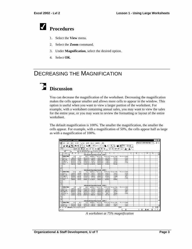
Discussion You can decrease the magnification of the worksheet. Decreasing the magnification makes the cells appear smaller and allows more cells to appear in the window. This option is useful when you want to view a larger portion of the worksheet. For example, with a worksheet containing annual sales, you may want to view the sales for the entire year, or you may want to review the formatting or layout of the entire worksheet. The default magnification is 100%. The smaller the magnification, the smaller the cells appear. For example, with a magnification of 50%, the cells appear half as large as with a magnification of 100%.
A worksheet at 75% magnification

Lesson 1 - Using Large Worksheets Excel 2002 - Lvl 2
Page 4 Organizational & Staff Development, U of T
Changing the magnification affects the screen display only. It does not affect the appearance of the printed worksheet.
You can also use the Zoom list on the Standard toolbar to change the magnification.
Procedures
1. Select the View menu.
2. Select the Zoom command.
3. Under Magnification, select the desired option.
4. Select OK.
CHANGING THE MAGNIFICATION OF A RANGE
Discussion You can magnify a selected range so that its size adjusts as needed to fit the worksheet window. It is useful to zoom selections when you want to view all the cells in a range at the same time. For example, with a worksheet containing annual sales, you may want to zoom in on the numbers that make up the annual sales.

Excel 2002 - Lvl 2 Lesson 1 - Using Large Worksheets
Organizational & Staff Development, U of T Page 5
Fitting a selection to the window
Procedures
1. Select the range for which you want to change the magnification.
2. Select the View menu.
3. Select the Zoom command.
4. Select the Fit selection option.
5. Select OK.
SWITCHING TO FULL SCREEN VIEW
Discussion You can view a worksheet without viewing screen elements such as toolbars and title bars using Full Screen view. This option allows you to display a large portion of a large worksheet. For example, you can use Full Screen view to display as much of an annual worksheet as possible, without changing the magnification.

Lesson 1 - Using Large Worksheets Excel 2002 - Lvl 2
Page 6 Organizational & Staff Development, U of T
Full Screen view
When viewing the worksheet in Full Screen view, a Full Screen toolbar appears. If you close the Full Screen toolbar, you must select the Full Screen command from the View menu to return to Normal view.
Procedures
1. Select the View menu.
2. Select the Full Screen command.
3. To return to Normal view, click the Close Full Screen button on the Full Screen toolbar.
SPLITTING THE WINDOW
Discussion If you need to view two or more areas of a large worksheet at the same time, you can split the workbook window into panes. Panes display different areas of the same
Excel 2002 - Lvl 2 Lesson 1 - Using Large Worksheets
Organizational & Staff Development, U of T Page 7
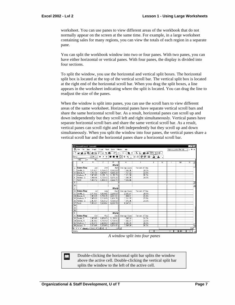
worksheet. You can use panes to view different areas of the workbook that do not normally appear on the screen at the same time. For example, in a large worksheet containing sales for many regions, you can view the totals of each region in a separate pane. You can split the workbook window into two or four panes. With two panes, you can have either horizontal or vertical panes. With four panes, the display is divided into four sections. To split the window, you use the horizontal and vertical split boxes. The horizontal split box is located at the top of the vertical scroll bar. The vertical split box is located at the right end of the horizontal scroll bar. When you drag the split boxes, a line appears in the worksheet indicating where the split is located. You can drag the line to readjust the size of the panes. When the window is split into panes, you can use the scroll bars to view different areas of the same worksheet. Horizontal panes have separate vertical scroll bars and share the same horizontal scroll bar. As a result, horizontal panes can scroll up and down independently but they scroll left and right simultaneously. Vertical panes have separate horizontal scroll bars and share the same vertical scroll bar. As a result, vertical panes can scroll right and left independently but they scroll up and down simultaneously. When you split the window into four panes, the vertical panes share a vertical scroll bar and the horizontal panes share a horizontal scroll bar.
A window split into four panes
Double-clicking the horizontal split bar splits the window above the active cell. Double-clicking the vertical split bar splits the window to the left of the active cell.

Lesson 1 - Using Large Worksheets Excel 2002 - Lvl 2
Page 8 Organizational & Staff Development, U of T
Procedures
1. To split the window into horizontal panes, drag the horizontal split box to the desired row.
2. To view different areas of the worksheet in the horizontal panes, click either vertical scroll bar.
3. To split the window into vertical panes, drag the vertical split box to the desired column.
4. To view different areas of the worksheet in the vertical panes, click either horizontal scroll bar.
REMOVING SPLIT WINDOWS
Discussion You can remove the panes from a workbook window by double-clicking the horizontal or vertical split bar. You can remove the panes when you no longer need to view distant areas of the worksheet. For example, after you have viewed the regional totals in a large sales worksheet, you may want to view only the figures for one region.
Procedures
1. To remove horizontal panes, double-click the horizontal split bar.
2. To remove vertical panes, double-click the vertical split bar.
FREEZING THE PANES
Discussion Occasionally a worksheet is so large, you cannot view the column or row headings and all the data at the same time. When this happens, it is difficult to view the headings for the data in the worksheet. For example, in a worksheet containing sales figures for several hundred sales representatives, you cannot view the column

Excel 2002 - Lvl 2 Lesson 1 - Using Large Worksheets
Organizational & Staff Development, U of T Page 9
headings and the representatives at the bottom of the list at the same time. To solve this problem, you can freeze worksheet titles in panes. Freezing panes prevents the row and column headings from scrolling out of view as you navigate the worksheet. Frozen panes are indicated by a line below a row and a line to the right of a column.
Frozen row and column headings
Procedures
1. To freeze both row and column headings, place the active cell in the cell directly below the column headings you want to freeze and to the right of the row headings you want to freeze.
2. Select the Window menu.
3. Select the Freeze Panes command.
UNFREEZING THE PANES
Discussion After you have frozen headings in a large worksheet, you can unfreeze the panes. Unfreezing removes the panes so that title rows or columns are no longer frozen on the screen.
Lesson 1 - Using Large Worksheets Excel 2002 - Lvl 2
Page 10 Organizational & Staff Development, U of T
Procedures
1. Select the Window menu.
2. Select the Unfreeze Panes command.

LESSON 2 - WORKING WITH MULTIPLE WORKSHEETS
In this lesson, you will learn how to:
• Use multiple worksheets
• Navigate between worksheets
• Select worksheets
• Rename worksheets
• Select multiple worksheets
• Color worksheet tabs
• Insert worksheets
• Delete worksheets
• Print selected worksheets

Lesson 2 - Working with Multiple Worksheets Excel 2002 - Lvl 2
Page 12 Organizational & Staff Development, U of T
USING MULTIPLE WORKSHEETS
Discussion Workbook files can contain multiple worksheets. Using multiple worksheets is a convenient way to manage related data in the same workbook. For example, you can enter sales data for individual months, quarters, or regions in separate worksheets. You also can create summary worksheets that add numbers from each of the worksheets in a workbook. In addition, you can group worksheets to apply consistent formatting, as well as to print all the worksheets as a group. By default, a new workbook contains three worksheets. The name of each worksheet appears on a tab above the status bar. The default name is Sheet, followed by a number. You can change the name to indicate the type of information on the worksheet. For example, if your worksheet contained your weekly expenses, you could rename the default worksheet Expenses. You can also add color to a worksheet tab. A workbook can contain up to 255 worksheets. Worksheets can be moved and copied within the current workbook.
A workbook with multiple worksheets
To change the number of default worksheets, select the General page in the Options dialog box.

Excel 2002 - Lvl 2 Lesson 2 - Working with Multiple Worksheets
Organizational & Staff Development, U of T Page 13
NAVIGATING BETWEEN WORKSHEETS
Discussion The active worksheet is the worksheet that is currently displayed. You can display a worksheet by clicking its tab; however, by default, only six worksheet tabs appear in the workbook window. If you have more than six worksheets, you cannot see all the worksheet tabs at one time. For example, in a workbook that contains worksheets for every month of the year, the tabs for the last few months of the year would be hidden, depending on how the months are named. If the worksheet tab you want to view is not visible, you can use the tab scrolling buttons to display hidden tabs.
Button Function
Displays the next worksheet tab to the right.
Displays the previous worksheet tab to the left.
Displays the last worksheet tab in the workbook.
Displays the first worksheet tab in the workbook.
You can drag the tab split box located to the left of the horizontal scroll bar as desired to display more or fewer tabs. You can double-click the tab split box to return the tab display to the default number of tabs.
Procedures
1. To view the next tab to the right, click the Next Tab button .
2. To view the next tab to the left, click the Previous Tab button .
3. To view the last worksheet tab, click the Last Tab button .
4. To view the first worksheet tab, click the First Tab button .
5. To view the contents of a worksheet, click the desired worksheet tab.

Lesson 2 - Working with Multiple Worksheets Excel 2002 - Lvl 2
Page 14 Organizational & Staff Development, U of T
SELECTING WORKSHEETS
Discussion You can select a worksheet at any time by displaying the sheet list. The sheet list contains the name of all the worksheets in a workbook. It is a convenient tool when using a workbook with a large number of worksheets. For example, in an annual workbook containing monthly worksheets, you can use the sheet list to quickly select and view the third month in each quarter, one at a time.
The sheet list
Procedures
1. Right-click any tab scrolling button.
2. Select the desired worksheet.

Excel 2002 - Lvl 2 Lesson 2 - Working with Multiple Worksheets
Organizational & Staff Development, U of T Page 15
RENAMING WORKSHEETS
Discussion You can replace the default worksheet names with descriptive names. For example, a worksheet containing January sales figures can be named January. Worksheet names can be up to 31 characters long, but cannot include colons (:), slash marks (/), backslashes (\), question marks (?), or asterisks (*). In addition, the name cannot be enclosed in square brackets ([]). Each worksheet name in a workbook must be unique.
Procedures
1. Double-click the worksheet tab you want to rename.
2. Type the desired worksheet name.
3. Press [Enter].
SELECTING MULTIPLE WORKSHEETS
Discussion Before you can apply a command to a worksheet, you must select the worksheet. If you select multiple worksheets, you can apply a command to all the worksheets at the same time. For example, you can copy, move, delete, and print all the worksheets in a selected group at the same time. In addition, when you insert new sheets, the number of sheets you select determines the number of sheets inserted.
To deselect a selected worksheet without deselecting the group, hold the [Ctrl] key and click the worksheet tab you want to deselect.
When multiple worksheets are selected, the text [Group] appears next to the title of the workbook.
To deselect worksheet tabs, click any unselected worksheet tab.

Lesson 2 - Working with Multiple Worksheets Excel 2002 - Lvl 2
Page 16 Organizational & Staff Development, U of T
Procedures
1. Click the tab of the first worksheet you want to select.
2. Hold [Shift] and click the tab of the last adjacent worksheet you want to select.
3. To add non-adjacent worksheets to the group, hold [Ctrl] and click the tab of each worksheet you want to add.
COLORING WORKSHEET TABS
Discussion Excel allows you to add color to worksheet tabs. If color has been added to a worksheet tab, a horizontal line of the selected color appears below the worksheet name while the tab is selected; the entire sheet tab displays the color whenever the tab is not selected. You can select single or multiple worksheets when adding color to worksheet tabs. For example, you may want to add the color red to all worksheets containing sales figures for the first quarter and add a different color for each of the second quarter worksheets.
Adding color to a worksheet tab

Excel 2002 - Lvl 2 Lesson 2 - Working with Multiple Worksheets
Organizational & Staff Development, U of T Page 17
You can also right-click a worksheet tab and select the Tab Color command from the shortcut menu to display the Format Tab Color palette.
Procedures
1. Select the worksheet tab to which you want to add a color.
2. Select the Format menu.
3. Point to the Sheet command.
4. Select the Tab Color command.
5. Select the desired color.
6. Select OK.
INSERTING WORKSHEETS
Discussion You can insert new worksheets into a workbook. For example, in a workbook containing worksheets for each month of the year, you can add worksheets for each quarter of the year. New worksheets are inserted to the left of the active worksheet. Excel gives new worksheets a default worksheet name, which you can change, if desired.
If you select multiple, adjacent worksheets, multiple worksheets are inserted. You cannot insert non-adjacent worksheets.
Procedures
1. Select the worksheet to the left of which you want to insert a new worksheet.
2. Select the Insert menu.
3. Select the Worksheet command.

Lesson 2 - Working with Multiple Worksheets Excel 2002 - Lvl 2
Page 18 Organizational & Staff Development, U of T
DELETING WORKSHEETS
Discussion You can delete unwanted worksheets. For example, you can delete a worksheet used for temporary calculations. When you delete a worksheet, the entire worksheet and the data it holds are permanently removed from the workbook.
If you select multiple worksheets, multiple worksheets are deleted.
If the worksheet you are deleting contains data, you will be prompted to confirm the deletion. You will not be prompted for a blank worksheet.
Procedures
1. Right-click the tab of the worksheet you want to delete.
2. Select the Delete command.
3. Select Delete, if prompted.
PRINTING SELECTED WORKSHEETS
Discussion You can print some or all the worksheets in a workbook. For example, in an annual workbook containing monthly worksheets, you may want to print only the worksheets for the most recent months. When printing one or more worksheets instead of the entire workbook, you must select the worksheets you want to print prior to opening the Print dialog box.

Excel 2002 - Lvl 2 Lesson 2 - Working with Multiple Worksheets
Organizational & Staff Development, U of T Page 19
Printing selected worksheets
You can print and preview the entire workbook by selecting the Entire workbook option in the Print dialog box.
After selecting the desired worksheets, you can see how they will look printed by clicking the Print Preview button on the Standard toolbar.
Procedures
1. Select the first worksheet you want to print.
2. Hold [Shift] and click the tab of the last adjacent worksheet you want to print.
3. Select the File menu.
4. Select the Print command.
5. Select the Active Sheet(s) option, if necessary.
6. Select OK.

LESSON 3 - MANAGING WORKSHEETS
In this lesson, you will learn how to:
• Copy worksheets
• Move worksheets
• Use grouped worksheets
• Move data between worksheets
• Copy data between worksheets
• Create 3-D formulas
• Use 3-D ranges in functions
Excel 2002 - Lvl 2 Lesson 3 - Managing Worksheets
Organizational & Staff Development, U of T Page 21
COPYING WORKSHEETS
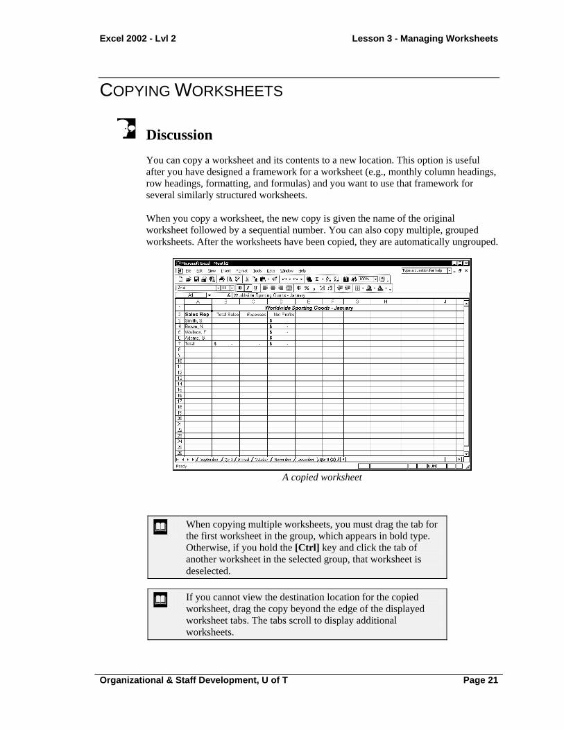
Discussion You can copy a worksheet and its contents to a new location. This option is useful after you have designed a framework for a worksheet (e.g., monthly column headings, row headings, formatting, and formulas) and you want to use that framework for several similarly structured worksheets. When you copy a worksheet, the new copy is given the name of the original worksheet followed by a sequential number. You can also copy multiple, grouped worksheets. After the worksheets have been copied, they are automatically ungrouped.
A copied worksheet
When copying multiple worksheets, you must drag the tab for the first worksheet in the group, which appears in bold type. Otherwise, if you hold the [Ctrl] key and click the tab of another worksheet in the selected group, that worksheet is deselected.
If you cannot view the destination location for the copied worksheet, drag the copy beyond the edge of the displayed worksheet tabs. The tabs scroll to display additional worksheets.

Lesson 3 - Managing Worksheets Excel 2002 - Lvl 2
Page 22 Organizational & Staff Development, U of T
Procedures
1. Select the tab of each worksheet you want to copy.
2. Hold [Ctrl] and drag the selected worksheet tabs to the desired location.
MOVING WORKSHEETS
Discussion You can move a worksheet to a new location in a workbook and still have it retain the same name and contents. Moving worksheets allows you to rearrange them or to place new worksheets in a desired location in the workbook. For example, in an annual workbook containing monthly worksheets, you may want to reorder the worksheets so that the first, second, and third months in each quarter are adjacent. You can also move multiple, grouped worksheets. After multiple grouped worksheets have been moved, they are automatically ungrouped.
Procedures
1. Select the tab of each worksheet you want to move.
2. Drag the selected worksheet tabs to the desired location.
USING GROUPED WORKSHEETS
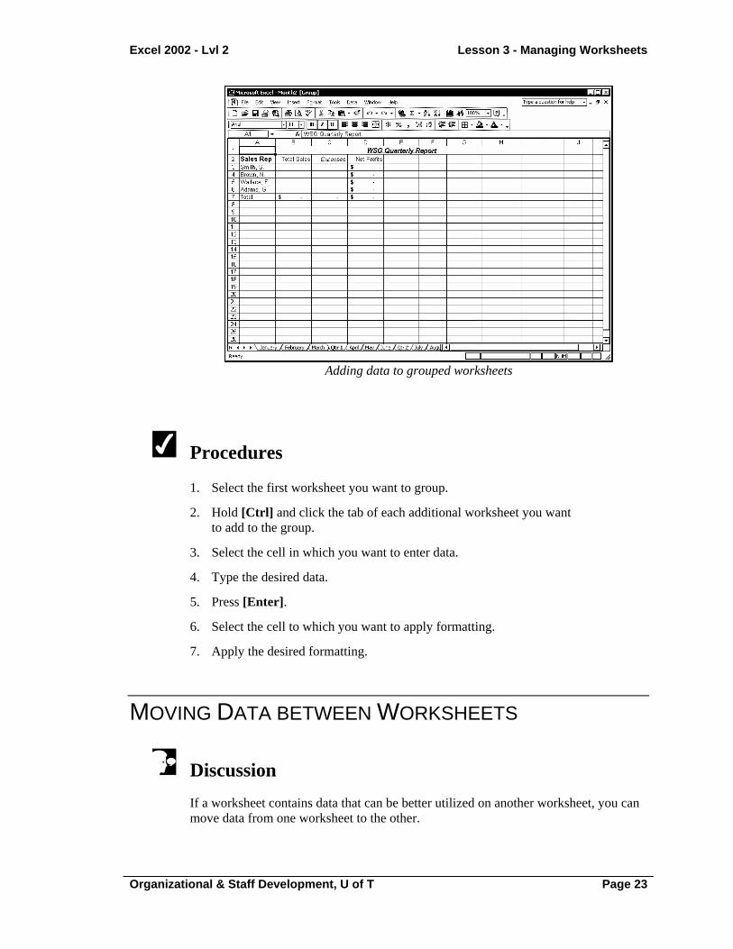
Discussion When multiple worksheets are selected, the worksheets are grouped. If you type, edit, create formulas, or format entries in one of the grouped worksheets, entries in the same cell in all the grouped worksheets change. Grouping is useful when you want to create the same structure and appearance in all the worksheets in a workbook. For example, when creating monthly worksheets in a workbook, you can group the worksheets so that you can enter and format all the column headings, row headings, and formulas in the group at one time.
Excel 2002 - Lvl 2 Lesson 3 - Managing Worksheets
Organizational & Staff Development, U of T Page 23
Adding data to grouped worksheets
Procedures
1. Select the first worksheet you want to group.
2. Hold [Ctrl] and click the tab of each additional worksheet you want to add to the group.
3. Select the cell in which you want to enter data.
4. Type the desired data.
5. Press [Enter].
6. Select the cell to which you want to apply formatting.
7. Apply the desired formatting.
MOVING DATA BETWEEN WORKSHEETS
Discussion If a worksheet contains data that can be better utilized on another worksheet, you can move data from one worksheet to the other.

Lesson 3 - Managing Worksheets Excel 2002 - Lvl 2
Page 24 Organizational & Staff Development, U of T
The most common reason for moving data is to break up a single large worksheet into several smaller ones. For example, if a workbook consists of one large worksheet containing data for each month of the year, you can move the monthly data to separate worksheets.
You can drag to move data between worksheets by holding the [Alt] key as you drag.
When you move data between worksheets, the Paste Options button may appear, allowing you to control how the data is pasted.
Procedures
1. Select the worksheet containing the data you want to move.
2. Select the cells you want to move.
3. Click the Cut button .
4. Select the destination worksheet.
5. Select the first cell in the paste range.
6. Click the Paste button .
COPYING DATA BETWEEN WORKSHEETS
Discussion You can copy data between worksheets, using the same techniques you use to copy and move data within a worksheet. For example, if one worksheet contains information you want to include on each worksheet in the workbook, you can copy the information as needed. When copying data between worksheets, formulas update to the new locations, just as they do when you copy information within a worksheet.

Excel 2002 - Lvl 2 Lesson 3 - Managing Worksheets
Organizational & Staff Development, U of T Page 25
You can also copy data to another worksheet by dragging. Select the data, press the [Ctrl] and [Alt] keys, and drag the selection by its border, first to the worksheet tab, and then when the worksheet appears, to the desired location.
When you copy data between worksheets, the Paste Options button may appear, allowing you to control how the data is pasted.
Procedures
1. Select the worksheet containing the data you want to copy.
2. Select the cells you want to copy.
3. Click the Copy button .
4. Select the destination worksheet.
5. Select the first cell in the paste range.
6. Click the Paste button .
CREATING 3-D FORMULAS
Discussion You can create formulas on one worksheet that refer to numbers on other worksheets in the same or different workbooks. You can use 3-D formulas to summarize data from all the worksheets in a workbook. For example, you can create quarterly worksheets in an annual workbook that summarize data from each month. Like all formulas, 3-D formulas update whenever the data used in the formula changes. In 3-D formulas, the worksheet names are separated from the cell address by an exclamation point (!). For example, the following formula adds the number in cell E3 in each of four quarterly worksheets:
=Qtr 1!E3+Qtr 2!E3+Qtr 3!E3+Qtr 4!E3

Lesson 3 - Managing Worksheets Excel 2002 - Lvl 2
Page 26 Organizational & Staff Development, U of T
A 3-D formula
Procedures
1. Select the worksheet in which you want to create a 3-D formula.
2. Select the cell in which you want to create the formula.
3. Type =.
4. Select the worksheet containing the data you want to use in the formula.
5. Select the cell containing the data you want to use in the formula.
6. Type the desired mathematical operator.
7. Select the worksheet containing the next piece of data you want to use in the formula.
8. Select the cell containing the data you want to use in the formula.
9. Continue adding mathematical operators and cell addresses as needed to complete the formula.
10. Press [Enter].

Excel 2002 - Lvl 2 Lesson 3 - Managing Worksheets
Organizational & Staff Development, U of T Page 27
USING 3-D RANGES IN FUNCTIONS
Discussion You can perform calculations on cells in multiple, adjacent worksheets by creating functions that use 3-D ranges. For example, you can use a 3-D range to sum the monthly totals that appear at the same cell address in multiple, adjacent worksheets. Since the function refers to the same cell address in adjacent worksheets, you can group the worksheets and then create the function. This technique can save time in creating functions such as SUM and AVERAGE. In formulas that contain 3-D ranges, the worksheet names are separated from the cell address by an exclamation point (!). For example, in the following formula, the SUM function adds the numbers in cell F3 in four quarterly worksheets:
=SUM(Qtr 1:Qtr 4!F3)
A 3-D range in a SUM function
Procedures
1. Select the worksheet in which you want to enter the function.
2. Select the cell in which you want to enter the formula.
3. Type =, followed by the function name and an open parenthesis ( ( ).

Lesson 3 - Managing Worksheets Excel 2002 - Lvl 2
Page 28 Organizational & Staff Development, U of T
4. Select the first worksheet containing the data you want to use in the function.
5. Select the cell that contains the data you want to use in the function.
6. Hold [Shift] and select the last worksheet you want to include in the 3-D range.
7. Type the closing parenthesis ( ) ).
8. Press [Enter].

LESSON 4 - USING PASTE OPTIONS
In this lesson, you will learn how to:
• Copy/Cut and paste data
• Use the Paste Options button
• Using the Paste list
• Use the Clipboard task pane

Lesson 4 - Using Paste Options Excel 2002 - Lvl 1
Page 30 Organizational & Staff Development, U of T
COPYING/CUTTING AND PASTING DATA
Discussion When you are creating a worksheet, you can save time by copying cell contents from one location to another. The Copy feature copies the selected cell contents to the Office Clipboard. The Paste feature pastes the contents from the Office Clipboard into the current selection on the worksheet. When you copy cells that contain text or numbers, Excel creates an exact copy of the contents when they are pasted to another location. When you copy cells containing formulas, Excel adjusts the cell references to the row or column where the formula is pasted. For example, if the formula =B1+B2+B3 calculates the total of three cells in column B and you copy that formula to the adjacent cell in column C, Excel adjusts the formula to =C1+C2+C3 so that the total of the three corresponding cells in column C are calculated. Excel assumes that the paste range exactly matches the copied range. For example, if the copied range consists of three cells, Excel assumes that the paste range will consist of three cells. As a result, you need only select the cell in the upper, left corner of the desired paste range to paste the entire copied range. If the copied range is a single cell and you select a paste range of multiple cells, the contents of the copied cell are pasted into each cell in the paste range. You can also use the Cut and Paste features to move cell contents on a worksheet. The Cut feature cuts the cell contents from the worksheet, placing them on the Office Clipboard. The Paste feature pastes the contents of the Office Clipboard into the current selection. The contents of the cut range are then deleted from the worksheet. When you move cells containing formulas, Excel does not adjust the cell references in the formulas. The formulas still refer to the original cells for the calculation. If you move both the formula and the cells containing the data, the cell references in the formula adjust to the new location of the data. The Paste button on the Standard toolbar provides a Paste list. Clicking the Paste arrow displays a list of paste options. You can choose to paste a formula, paste the resulting value of a formula, paste a link, paste data without border formatting, or transpose a range of cells from a horizontal range to a vertical range or vice versa. After an item has been pasted, the Paste Options button appears in the document next to the pasted text. You can use paste options to choose whether source or destination formatting should be applied, or you can press the [Esc] key to hide the button.

Excel 2002 - Lvl 1 Lesson 4 - Using Paste Options
Organizational & Staff Development, U of T Page 31
Copying and pasting data
A blinking marquee remains around the copied range after it has been pasted to let you know which cells were copied. Pressing the [Esc] key removes the blinking marquee.
If the Office Clipboard is set to appear automatically, the Clipboard task pane appears as soon as a second item is cut or copied.
You should be careful when pasting data into a range, because pasting overwrites any existing cell contents in that range.
Procedures
1. Select the cell you want to copy.
2. Click the Copy button on the Standard toolbar.
3. Select the range into which you want to paste the cell contents.
4. Click the Paste button on the Standard toolbar.

Lesson 4 - Using Paste Options Excel 2002 - Lvl 1
Page 32 Organizational & Staff Development, U of T
5. Select the cell you want to cut.
6. Click the Cut button on the Standard toolbar.
7. Select the range into which you want to paste the cell contents.
8. Click the Paste button on the Standard toolbar.
USING THE PASTE OPTIONS BUTTON
Discussion The Paste Options button appears on the worksheet adjacent to the pasted cell or range of cells after you have pasted a cut or copied item. Paste options allow you to decide how formatting differences should be applied to the pasted cells. It also allows you to link the pasted data to the original cut or copied cell, if desired. The available commands are determined by the data being pasted. When copying formatted text, you can select the Keep Source Formatting option to paste the text with its original formatting. When the Match Destination Formatting option is selected, the formatting in the paste location is applied to the pasted text. When pasting numeric data or a copied formula, you have additional options, such as pasting both values and source formatting, formatting only, or values only. You can hide the Paste Options button by pressing the [Esc] key.
The Paste Options list

Excel 2002 - Lvl 1 Lesson 4 - Using Paste Options
Organizational & Staff Development, U of T Page 33
The Paste Options button can be turned off by selecting the Tools menu and the Options command. In the Option dialog box, select the Edit page and deselect the Show Paste Options buttons option.
Procedures
1. Select the cell or range you want to move or copy.
2. Cut or copy the cells as desired.
3. Select the cell or range into which you want to paste the cut or copied contents.
4. Click the Paste button .
5. Click the Paste Options button .
6. Select the desired option.
7. To hide the Paste Options button, press [Esc].
USING THE PASTE LIST
Discussion When you copy text, numbers, or formulas, you can use the Paste button to paste the data into a new location. However, you can also use the Paste list to select other options for pasting text and formulas. The Formulas command is the default paste command for the Paste button. Formulas are pasted into the new location and, if the referenced data is also copied, cell references are changed. You can use the Values command to paste the results of a formula rather than the formula itself into a cell. This is useful if you want to paste just the current value of a formula and do not want the pasted data to be affected by new changes made to the original cell references. The No Borders command allows you to copy a cell with borders and paste the contents of the cell without borders.

Lesson 4 - Using Paste Options Excel 2002 - Lvl 1
Page 34 Organizational & Staff Development, U of T
The Transpose command is used to switch a vertical range of cells to a horizontal range or visa versa. For example, you can copy the row headings in column A and transpose them to create column headings across row 15. The Paste Link command pastes a link to the copied cell. If you paste cell B9 into cell D15 and select the Paste Link command, Excel pastes the link =$B$9 into cell D15. Thereafter, cell D15 will always display the same value as cell B9.
The Paste list
The Paste Special command in the Paste list opens the Paste Special dialog box, which provides additional options for pasting formats and data, and combining values.
Procedures
1. Select the cells you want to cut or copy.
2. Cut or copy the data as desired.
3. Select the cell or range into which you want to paste the cut or copied contents.
4. Click the arrow on the Paste button .

Excel 2002 - Lvl 1 Lesson 4 - Using Paste Options
Organizational & Staff Development, U of T Page 35
5. Select the desired command.
USING THE CLIPBOARD TASK PANE
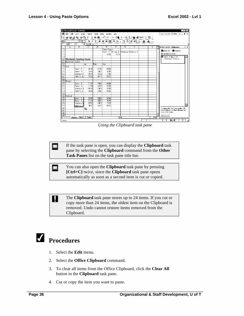
Discussion The Office Clipboard stores multiple cut or copied items, including graphics, from various worksheets or other Windows programs. You can then paste the items into one or more worksheets. The Office Clipboard is accessed by opening the Clipboard task pane. When you first open the Clipboard task pane, it displays the last item cut or copied to the Windows Clipboard. As you continue to cut or copy items, they are collected on the Clipboard task pane and remain available to all Office XP products. For each of the cut or copied items, the Clipboard task pane displays an icon and a portion of the text. You can click an item to paste it at the insertion point, or you can use the Paste All button to paste all the items at once. Right-clicking an item displays a shortcut menu containing options to paste or delete the item. After pasting text, the Paste Options button appears in the worksheet, allowing you to control the formatting of the pasted item. Once you have finished a particular copying sequence, you can clear the Office Clipboard of all items by clicking the Clear All button in the Clipboard task pane. In addition, the Office Clipboard clears automatically when you close all Office XP programs. You can continue pasting text or numbers to different locations by clicking the item in the Clipboard task pane. Formulas, however, are not copied to the Office Clipboard; only the result of the formula is copied. Therefore, you can use the Clipboard task pane only to paste the resulting value into the destination cell, not the formula itself.
Lesson 4 - Using Paste Options Excel 2002 - Lvl 1
Page 36 Organizational & Staff Development, U of T
Using the Clipboard task pane
If the task pane is open, you can display the Clipboard task pane by selecting the Clipboard command from the Other Task Panes list on the task pane title bar.
You can also open the Clipboard task pane by pressing [Ctrl+C] twice, since the Clipboard task pane opens automatically as soon as a second item is cut or copied.
The Clipboard task pane stores up to 24 items. If you cut or copy more than 24 items, the oldest item on the Clipboard is removed. Undo cannot restore items removed from the Clipboard.
Procedures
1. Select the Edit menu.
2. Select the Office Clipboard command.
3. To clear all items from the Office Clipboard, click the Clear All button in the Clipboard task pane.
4. Cut or copy the item you want to paste.

Excel 2002 - Lvl 1 Lesson 4 - Using Paste Options
Organizational & Staff Development, U of T Page 37
5. Select the cell into which you want to paste the item.
6. Point to the item you want to paste in the Clipboard task pane.
7. Click the item to paste it into the current cell.
8. To paste all the items in the Clipboard task pane, click the Paste All button.
9. To remove an item from the Clipboard, right-click it in the Clipboard task pane.
10. Select the Delete command.

LESSON 5 - USING RANGE NAMES
In this lesson, you will learn how to:
• Work with range names
• Jump to a named range
• Assign names
• Use range names in formulas
• Create range names from headings
• Apply range names
• Delete range names
• Use range names in 3-D formulas
• Create 3-D range names
• Use 3-D range names in formulas

Excel 2002 - Lvl 2 Lesson 5 - Using Range Names
Organizational & Staff Development, U of T Page 39
WORKING WITH RANGE NAMES
Discussion You can assign a name to a cell or a range in a worksheet. Once a name has been assigned, the name can be used in any instance where you can use a cell address. For example, you can use names for ranges in dialog boxes and formulas. Advantages to using names instead of cell addresses include:
1. Names reduce the chance of error in formulas. It is easy to
recognize if the name EXPENSES is typed incorrectly. If a cell or range address is typed incorrectly, it is harder to detect.
2. Names adapt to changes within a range (for example, when rows and columns are added to or removed from the range).
3. Names are easy to recognize and maintain in formulas. For example, the formula =TOTALSALES-EXPENSES is easier to understand than the formula =E3-F3.
4. You can easily move the active cell to a named cell or range using the Name box.
5. Names created in one worksheet are available to all other worksheets in the workbook.
6. Names can refer to non-contiguous ranges or to ranges that contain blank cells, columns, or rows.
7. Names are absolute. If you use a name in a formula, the formula always refers to that range, even if you copy or move the formula.
You can use names to refer to cells, ranges, multiple ranges, and ranges in other worksheets.
JUMPING TO A NAMED RANGE
Discussion You can use a name to move quickly to a cell or a range. Since a name assigned in a worksheet is available in all worksheets in the workbook, you can use names to move easily between the worksheets. For example, in a workbook containing worksheets for different products, you can quickly jump to the desired product worksheet using the name assigned to it.

Lesson 5 - Using Range Names Excel 2002 - Lvl 2
Page 40 Organizational & Staff Development, U of T
You use the Name Box list to jump to a named range. The Name Box list is located at the left end of the formula bar and displays all the assigned names in a workbook. When you choose a name from the Name Box list, the range is selected and the active cell appears in the first cell of the range.
Jumping to a named range
If the formula bar is not displayed, you can use the View menu to view it.
Procedures
1. Click the arrow for the Name Box list on the formula bar.
2. Select the name of the desired range.
ASSIGNING NAMES
Discussion You can use names instead of cell references in formulas and dialog boxes. For example, if you are summing totals from several worksheets, you can assign names to

Excel 2002 - Lvl 2 Lesson 5 - Using Range Names
Organizational & Staff Development, U of T Page 41
the totals in each worksheet and then use the range names in the formula instead of the cell addresses. You can use the Name Box to assign range names. The following rules apply to naming ranges:
1. Names must start with a letter or an underscore. The remainder of the
name can contain any character except a space or a hyphen. Avoid using the dollar sign ($), since it may be confused with an absolute reference.
2. Names can be up to 255 characters long. You should keep them short to make them easy to use and to conserve space in formulas (which also have a maximum length of 255 characters).
3. Names are not case-sensitive. They can be typed in either uppercase or lowercase.
4. You should not use names that resemble cell references (such as Q1).
Assigning a name to a cell
Procedures
1. Select the cell or range you want to name.
2. Click in the Name Box on the formula bar.
3. Type the desired name.

Lesson 5 - Using Range Names Excel 2002 - Lvl 2
Page 42 Organizational & Staff Development, U of T
4. Press [Enter].
USING RANGE NAMES IN FORMULAS
Discussion You can use a name rather than a cell address in a formula. Using a name in a formula makes the formula easier to read and understand. For example, it is easy to understand what information the following formula calculates; =INCOME-EXPENSES. If the named cells change, the formula automatically updates. Since names are absolute, you can use a name in place of an absolute cell reference in a formula. For example, if you are calculating a percentage of a range named Total, the formula will always refer to the Total range if you use the name rather than the cell address, no matter where you move or copy the formula.
Using range names in a formula
You can also select a name from the Paste Name dialog box to insert a name into a formula. To use the Paste Name dialog box, begin the formula. When you need to reference the name in the formula, press the [F3] key and double-click the desired name.

Excel 2002 - Lvl 2 Lesson 5 - Using Range Names
Organizational & Staff Development, U of T Page 43
You can also access the Paste Name dialog box while creating a formula by selecting the Insert menu, the Name command and the Paste command.
Procedures
1. Select the cell in which you want the result of the formula to appear.
2. Start typing the formula or function.
3. Type the desired name at the appropriate location in the formula.
4. Complete the formula.
5. Press [Enter].
CREATING RANGE NAMES FROM HEADINGS
Discussion You can create names for rows and columns using text entered into the first or last cell of the row or the top or bottom cell of the column. This option is a quick way to create names that correspond directly to worksheet entries. For example, in a worksheet containing the quantity of products sold each month, you can use the product names in the row headings to name the rows of quantities sold. When Excel names rows and columns from headings, it uses the text in the indicated location (i.e., the top, bottom, right or left cell) to name the selected range. The cells containing the text are not included in the named ranges. You can create multiple names at the same time by selecting a range that spans several columns or rows.

Lesson 5 - Using Range Names Excel 2002 - Lvl 2
Page 44 Organizational & Staff Development, U of T
Creating range names from headings
Although the text in the header columns and rows is not included in the named ranges, it must be included in the range you select prior to performing the command in order for Excel to determine the range names.
Procedures
1. Select the range you want to name, as well as the row or column heading containing the desired range names.
2. Select the Insert menu.
3. Point to the Name command.
4. Select the Create command.
5. Under Create names in, select the option corresponding to the location of the desired names.
6. Select OK.

Excel 2002 - Lvl 2 Lesson 5 - Using Range Names
Organizational & Staff Development, U of T Page 45
APPLYING RANGE NAMES
Discussion After you have named a range, you can use it in existing formulas. For example, after you have created formulas in a worksheet, you may decide that using names in the formulas will make it easier for others to analyze the worksheet. Since Excel does not automatically replace cell references in existing formulas when you assign names, you must replace the cell addresses in existing formulas with names as desired. This technique is called applying names. Names are applied to the current worksheet only. Consequently, you cannot group worksheets and apply names to multiple sheets at the same time.
Applying range names
If you want to apply names throughout a worksheet, you can select a single cell in the worksheet.
Excel uses an underscore ( _ ) for blank spaces in a range name. For example, the heading Total Sales will be assigned the range name Total_Sales.

Lesson 5 - Using Range Names Excel 2002 - Lvl 2
Page 46 Organizational & Staff Development, U of T
Some names in the Apply Names dialog box may already be selected. Be sure to deselect the names you do not want to apply. Click once on a selected name to deselect it.
Procedures
1. Select the range in which you want to apply names.
2. Select the Insert menu.
3. Point to the Name command.
4. Select the Apply command.
5. Select the names you want to apply in the Apply names list box, if necessary.
6. Select OK.
DELETING RANGE NAMES
Discussion You can delete names you no longer use. For example, if you change the name of a range, you can delete the old name. Deleting a name permanently removes it from the workbook. If you accidentally delete a name to which a formula refers, the formula can no longer calculate correctly; the error message #NAME? appears in the cell instead of the result of the formula, and the Error Checking button appears next to the cell containing the error message.
If you inadvertently delete a name used in a formula, you can redefine that name to make the formula accurate again.
You can click the Error Checking button for more information about the error. The name of the error appears at the top of the list and is highlighted in gray. Selecting the Help on this error command opens the Microsoft Help window to the pertinent error topic.

Excel 2002 - Lvl 2 Lesson 5 - Using Range Names
Organizational & Staff Development, U of T Page 47
Procedures
1. Select the Insert menu.
2. Point to the Name command.
3. Select the Define command.
4. Select the name you want to delete from the Names in workbook list box.
5. Select Delete.
6. Select Close.
USING RANGE NAMES IN 3-D FORMULAS
Discussion A 3-D formula is a formula where cell references refer to cells in more than one worksheet. In standard 3-D formulas, you must activate each worksheet and select the cells you want to reference as you are building the formula. You can use range names as a simple and effective way to create 3-D formulas. Since names are available to all worksheets in the workbook, you can select names from the Name Box list or type them into the formula rather than going to each worksheet to select cell references. This option can save you time and reduce confusion in creating 3-D formulas. Names are often easier to remember than cell addresses, particularly in a large worksheet or in multiple workbooks when you cannot see the desired cell. When using names in formulas, you can either type the name into the formula or select the name from the Paste Name dialog box. If range names are long, the Paste Name dialog box helps you avoid typing errors.

Lesson 5 - Using Range Names Excel 2002 - Lvl 2
Page 48 Organizational & Staff Development, U of T
Using range names in a 3-D formula
If you make a typing error or misspell a name, the #NAME? error appears in the cell.
Procedures
1. Select the worksheet in which you want to create the formula.
2. Select the cell in which you want to create the formula.
3. Type = to start the formula.
4. Press [F3].
5. Double-click the desired name.
6. Type the desired mathematical operator.
7. Enter names and mathematical operators as necessary to complete the formula.
8. Press [Enter].

Excel 2002 - Lvl 2 Lesson 5 - Using Range Names
Organizational & Staff Development, U of T Page 49
CREATING 3-D RANGE NAMES
Discussion You can create names that refer to the same range in multiple worksheets. For example, you can define a name for the same cell address in four different worksheets. Naming a 3-D range can simplify creating a formula.
Creating a 3-D range name
Names that refer to 3-D ranges do not appear in the Name Box. They do appear in the Paste Name dialog box.
Procedures
1. Select the Insert menu.
2. Point to the Name command.
3. Select the Define command.
4. Type the desired range name.
5. Under Refers to, click the Collapse Dialog button .
6. Go to the first worksheet of the group you want to name.
7. Hold [Shift] and click the tab of the last worksheet you want to include in the group.
8. Select the range you want to name.

Lesson 5 - Using Range Names Excel 2002 - Lvl 2
Page 50 Organizational & Staff Development, U of T
9. Click the Expand Dialog button .
10. Select Add.
11. Select OK.
USING 3-D RANGE NAMES IN FORMULAS
Discussion You can use a named 3-D range in a formula just as you would any other named range. 3-D ranges can save you a significant amount of time. For example, if you have named the cell containing the quarterly totals in each of four worksheets, you can sum all four cells using the range name.
Using a 3-D range name in a formula
Procedures
1. Select the cell in which you want to create the formula.
2. Type =, the function name, and an open parenthesis ( ( ).
3. Type the 3-D range name you want to reference.

Excel 2002 - Lvl 2 Lesson 5 - Using Range Names
Organizational & Staff Development, U of T Page 51
4. Type any additional information needed to complete the function and then type the closing parenthesis ( ) ).
5. Press [Enter].

LESSON 6 - CREATING SIMPLE FORMULAS
In this lesson, you will learn how to:
• Use formulas
• Enter formulas
• Use functions
• Enter basic functions
• Insert functions in formulas
• Edit functions
• Use the AutoCalculate feature
• Use range borders to modify formulas
• Check errors

Excel 2002 - Lvl 1 Lesson 6 - Creating Simple Formulas
Organizational & Staff Development, U of T Page 53
USING FORMULAS
Discussion Formulas are used to perform calculations on values entered into the cells of a worksheet. They consist of the addresses of the cells containing the values and the appropriate mathematical operators. Formulas always begin with an equal sign (=) because they contain cell addresses. The equal sign prevents Excel from interpreting the formula as text, since cell addresses begin with letters. For example, to add the numbers in cells A1 and A2, you would type the formula =A1+A2. You enter the formula in the cell where you want the result to appear. Since formulas use cell addresses, they automatically recalculate whenever the value in any cell used in the formula changes. When a cell containing a formula is selected, the formula appears in the formula bar and the calculated results of the formula appear in the cell. The mathematical operators that can be used in a formula are listed in the following table:
Operator Performs
+ (plus sign) Addition
- (minus sign) Subtraction
* (asterisk) Multiplication
/ (slash) Division
( ) (parentheses) Controls the order of mathematical operations; calculations within parentheses are performed first
% (percent) Converts a number into a percentage; for example, when you type 10%, Excel reads the value as .10
^ (caret) Exponentiation; for example, when you type 2^3, Excel reads the value as 2*2*2
When more than one operator appears in a formula, it is calculated using the standard mathematical order of precedence. This order determines which operations are carried out first. The order of precedence is as follows: parentheses, exponentiation, multiplication and division, addition and subtraction. For example, the result of (8*7)+2 is 58, but the result of 8*(7+2) is 72.

Lesson 6 - Creating Simple Formulas Excel 2002 - Lvl 1
Page 54 Organizational & Staff Development, U of T
When multiplication and division or addition and subtraction appear in the same formula, they are evaluated from left to right as they appear in the formula.
Excel provides an AutoCorrect feature to help you correct formulas that contain errors. AutoCorrect identifies and offers suggestions on the most common mistakes made when entering formulas. For example, if a formula is entered as =A1+B1+, AutoCorrect will suggest the formula =A1+B1. If an error is found, you can either accept the correction provided or correct the formula yourself.
ENTERING FORMULAS
Discussion Formulas begin with an equal sign (=) because they contain cell addresses. The equal sign prevents Excel from interpreting the formula as text, since all cell addresses begin with letters. You enter a formula in the cell where you want the result to appear. When you enter a formula into a cell, you can either type the cell addresses referenced or use the mouse to select the cells and allow Excel to enter the cell addresses into the formula automatically. If the cell addresses that comprise a formula are not visible, it is more accurate to use the mouse to select the cell references while creating a formula. You only need to type the equal sign (=) to start the formula and then each of the arithmetic operators in the formula when appropriate. As you type or select cell addresses, Excel places a colored border with squares at each corner around each referenced cell. Excel uses a different color border for each cell referenced in the formula.

Excel 2002 - Lvl 1 Lesson 6 - Creating Simple Formulas
Organizational & Staff Development, U of T Page 55
Entering a formula
You can display the actual text entry entered into a cell (whether it is a number, label, or formula) by selecting the Tools menu, the Options command, and then the Formulas option on the View page. This option is useful as a teaching tool or when auditing a worksheet for formula errors.
Procedures
1. Select the cell into which you want to enter the formula.
2. Type an equal sign (=) to begin the formula.
3. Enter the first cell referenced in the formula.
4. Enter the first mathematical operator.
5. Enter the next cell referenced in the formula.
6. Continue entering cell references and mathematical operators as needed.
7. When you have finished creating the formula, press [Enter].

Lesson 6 - Creating Simple Formulas Excel 2002 - Lvl 1
Page 56 Organizational & Staff Development, U of T
USING FUNCTIONS
Discussion Excel has built-in functions that are shortcuts for formulas. Functions are special prewritten formulas that perform an operation on values or ranges of values and return the result to a cell in the worksheet. You can use functions to simplify and shorten formulas in your worksheets, especially those that perform lengthy or complex calculations. Examples of functions include:
=SUM(B5:B8) =AVERAGE(B5:B8) =PMT(.08,C8,85000) =ROUND(B5,2)
A function always starts with an equals sign (=) followed by the function's name and, enclosed in parentheses, its arguments. The function uses the arguments in its calculations. Arguments can be cell addresses, values, labels, or a combination of these; you can even use other functions or formulas as arguments. Functions are most commonly used to perform calculations on a range of cells. For example, it is easier to use the =SUM(A1:A7) function to add the numbers in cells A1 through A7 than to type the formula =A1+A2+A3+A4+A5+A6+A7. When you use a function, Excel provides help in the form of a function tooltip. The tooltip displays the structure of the function (i.e., the function name and the order of its required arguments).
ENTERING BASIC FUNCTIONS
Discussion Although the AutoSum list assists you in creating formulas for the most commonly used functions, you may want to manually enter a function. The SUM, AVERAGE, MAX, MIN, and COUNT functions are entered with the same syntax, including beginning the function with an equal sign (=) and then typing the name of the function and an open parenthesis. You then enter the cell range by dragging to select the cells or by typing the first and last cells in the range. These functions are defined in the following table:

Excel 2002 - Lvl 1 Lesson 6 - Creating Simple Formulas
Organizational & Staff Development, U of T Page 57
Function Syntax Description
SUM =SUM(A1:A20) Totals all the numbers in a range
AVERAGE =AVERAGE(A1:A20) Returns the average of a range of numbers; if a cell in the range is empty, it is not used in calculating the average; if a cell in the range contains the number zero, it is used in calculating the average
MAX =MAX(A1:A20) Returns the highest value in a range of numbers
MIN =MIN(A1:A20) Returns the lowest value in a range of numbers
COUNT =COUNT(A1:A20) Returns the number of cells in the range that contain numbers
Entering a basic function
You can enter a period (.) in place of a colon (:) when you are typing a function into a cell. When you press the [Enter] key, Excel automatically replaces the period (.) with a colon (:).

Lesson 6 - Creating Simple Formulas Excel 2002 - Lvl 1
Page 58 Organizational & Staff Development, U of T
The name of a function is not case-sensitive. For example, you can type SUM, Sum, or sum into a cell.
If you do not type the ending parenthesis when entering a function, Excel will add it for you.
Procedures
1. Select the cell into which you want to enter the formula.
2. Type the desired formula.
3. Press [Enter].
INSERTING FUNCTIONS IN FORMULAS
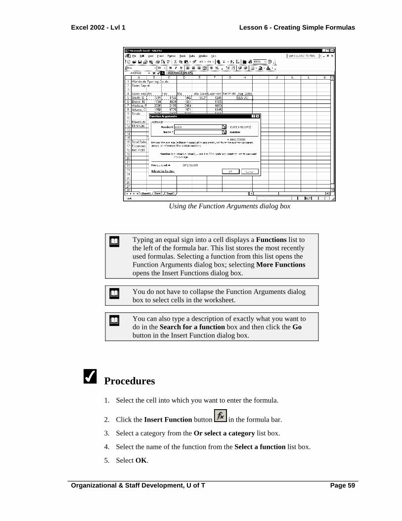
Discussion If you are not sure of the proper syntax of a function or if you need help entering a function into a formula, you can click the Insert Function button in the formula bar. The Insert Function button aids you in selecting the proper function. The functions in the Insert Function dialog box are grouped by category. Selecting a category displays only the functions within that category. If you do not know the category, you can select the All option to display all the available functions in alphabetical order. When you highlight a function, its structure and description appear below the Select a function list. After you have selected the desired function, the Function Arguments dialog box opens and displays an edit box for each argument in the function. You can enter a cell address, cell range, or numerical value for each argument into the corresponding edit box. An explanation of the selected function and an explanation of the selected argument appear below the list of edit boxes. As you fill in the arguments, the result of the formula appears below these explanations. Each edit box contains a Collapse Dialog button, which can be clicked to collapse the Function Arguments dialog box to a title bar so that you can see the worksheet. You can then select the desired cell range, which appears in the collapsed edit box. After selecting the range in the worksheet, you can then use the Expand Dialog button to redisplay the full dialog box. You can request help by selecting the Help on this function hyperlink in the Insert Function or Function Arguments dialog box.
Excel 2002 - Lvl 1 Lesson 6 - Creating Simple Formulas
Organizational & Staff Development, U of T Page 59
Using the Function Arguments dialog box
Typing an equal sign into a cell displays a Functions list to the left of the formula bar. This list stores the most recently used formulas. Selecting a function from this list opens the Function Arguments dialog box; selecting More Functions opens the Insert Functions dialog box.
You do not have to collapse the Function Arguments dialog box to select cells in the worksheet.
You can also type a description of exactly what you want to do in the Search for a function box and then click the Go button in the Insert Function dialog box.
Procedures
1. Select the cell into which you want to enter the formula.
2. Click the Insert Function button in the formula bar.
3. Select a category from the Or select a category list box.
4. Select the name of the function from the Select a function list box.
5. Select OK.

Lesson 6 - Creating Simple Formulas Excel 2002 - Lvl 1
Page 60 Organizational & Staff Development, U of T
6. Click the Number 1 edit box Collapse Dialog button .
7. Select the range you want to use in the calculation.
8. Click the Expand Dialog button .
9. Select OK.
EDITING FUNCTIONS
Discussion The Function Arguments dialog box simplifies creating functions by clearly listing each necessary argument. You can also open the Function Arguments dialog box to edit the arguments of an existing function.
Editing a function
Procedures
1. Select the cell containing the function you want to edit.
2. Click the Insert Function button in the formula bar.

Excel 2002 - Lvl 1 Lesson 6 - Creating Simple Formulas
Organizational & Staff Development, U of T Page 61
3. Select the Collapse Dialog button for the argument you want to edit.
4. Drag the range you want to use in the calculation.
5. Click the Expand Dialog button .
6. Select OK.
USING THE AUTOCALCULATE FEATURE
Discussion The AutoCalculate feature performs a simple calculation on a selected range of cells without making you supply a formula. The result of the calculation appears on the status bar. AutoCalculate results are temporary and are not placed in the worksheet. AutoCalculate is helpful when you want to spot-check your worksheet for accuracy or need a quick answer to a basic calculation. The AutoCalculate functions are accessed by right-clicking the AutoCalculate box located on the status bar. The AutoCalculate functions and their results are listed in the following table:
Function AutoCalculate Result
None Does not display a number
Average Displays the average of the cells in the selected range
Count Displays the number of cells in the selected range
Count Nums Displays the number of cells in the selected range that contain numeric entries
Max Displays the highest cell value in the selected range
Min Displays the lowest cell value in the selected range
Sum Displays the sum of the cells in the selected range

Lesson 6 - Creating Simple Formulas Excel 2002 - Lvl 1
Page 62 Organizational & Staff Development, U of T
Using AutoCalculate
Except for the Count function, AutoCalculate ignores all cells that do not contain a numeric entry.
AutoCalculate can also calculate multiple, selected ranges.
Procedures
1. Select the range you want to use in the calculation.
2. Right-click the AutoCalculate box on the status bar.
3. Select the desired function.
USING RANGE BORDERS TO MODIFY FORMULAS
Discussion When you create or edit a formula, Excel identifies its range references by displaying them with differently colored borders, with square handles at each corner.

Excel 2002 - Lvl 1 Lesson 6 - Creating Simple Formulas
Organizational & Staff Development, U of T Page 63
You can change the arguments in a formula by dragging a range border to include a different group of cells. You can move the range border to reference an entirely different range, or you can change the size of the border to include more or fewer cells. When you modify a range border, the corresponding range reference(s) in the formula change accordingly.
Using range borders to modify a formula
Procedures
1. Double-click the cell containing the formula you want to edit.
2. To move a range reference, drag its colored border to include the new range.
3. To change the size of a referenced range, drag the square range handle at any corner of the border in the desired direction to include more or fewer cells.
4. Press [Enter].

Lesson 6 - Creating Simple Formulas Excel 2002 - Lvl 1
Page 64 Organizational & Staff Development, U of T
CHECKING ERRORS
Discussion Excel provides an error checking feature that automatically checks your formulas against a pre-existing set of rules. If a formula breaks a rule, an error indicator appears in the form of a colored triangle in the corner of the cell containing the suspect formula. The error checking feature compares formulas to preset rules. The rules include checking to see if a number is stored as text, if a formula uses a range that is inconsistent with the formulas next to it, or if the formula omits a cell in a continuous range. When you click a cell with a green triangle in the upper left corner, the Trace Error button appears next to the cell. Pointing to the Trace Error button displays the reason the formula was flagged. Clicking the Trace Error button displays a list of error checking options from which you can choose to correct the error. Error checking options include selecting a suggested option to correct the error, getting an explanation of the error from Excel’s help system, ignoring the error, viewing the error checking options, and showing the Formula Auditing toolbar.
Using error checking options
The triangles and buttons that appear next to cells are also called smart tags.

Excel 2002 - Lvl 1 Lesson 6 - Creating Simple Formulas
Organizational & Staff Development, U of T Page 65
You can also view the error checking options by selecting the Tools menu, the Options command, and the Error Checking page. The automatic color for the triangle indicator is green, but you can use the Error Indicator Color list to select a different color.
Procedures
1. Select the cell with the green triangle in the upper, left corner.
2. Point to the Trace Error button to see why the formula was identified as an error.
3. Click the Trace Error button to view the error checking options.
4. Select the desired option.

LESSON 7 - WORKING WITH LABELS IN FORMULAS
In this lesson, you will learn how to:
• Use labels in formulas
• Use labels to define a range
• Use multiple stacked headings
• Refer to individual cells

Excel 2002 - Lvl 3 Lesson 7 - Working with Labels in Formulas
Organizational & Staff Development, U of T Page 67
USING LABELS IN FORMULAS
Discussion In formulas, you can refer to a cell or a range of cells using column and/or row headings. Formulas that use column or row headings to define a cell or range of cells are called natural language formulas. In Excel, row and column headings are called labels. Labels provide an efficient means of performing calculations using already existing names in the worksheet. You can use labels to refer to a cell or range of cells without actually creating a named range. In formulas, you can use the labels in the column heading to name the range of cells below the heading, those in the row heading to name the range of cells to the right of the heading, and those in both the column and row headings to refer to a specific cell (located at the intersection of the specified column and row). In addition, you can use multiple labels to refer to a range of cells.
You cannot use a label to refer to cells in another worksheet.
Labels are not case dependent. You can type jan to refer to the Jan label.
USING LABELS TO DEFINE A RANGE
Discussion You can use labels in formulas to perform calculations on columns or rows of numbers. Formulas that use labels as references are called natural language formulas. Excel recognizes column and row headings as labels. For example, if a column of numbers has the heading January, you can add the numbers in the column by typing =SUM(January). A label refers only to those cells below the column heading or to the right of the row heading before the first blank cell. Any cells beyond the blank cell are not included in the range. If you enter a label that appears more than once in the same worksheet, Excel prompts you to identify the label to which you are referring.

Lesson 7 - Working with Labels in Formulas Excel 2002 - Lvl 3
Page 68 Organizational & Staff Development, U of T
Labels in formulas act as relative references. That is, when you copy a formula using labels and paste it into a new location, the formula adjusts the label to the new location. For example, when you copy the formula =SUM(January) to the corresponding cell below the column heading February, the formula changes to =SUM(February).
Using a label in a formula to define a range
If you use a label in a formula that is the same as a named range in the workbook, the formula may not work properly.
Procedures
1. Select the cell in which you want to create the formula.
2. Start typing the formula or function.
3. Type the label in the column or row heading of the cell or range you want to use in the formula.
4. Type the remainder of the formula as needed.
5. Press [Enter].
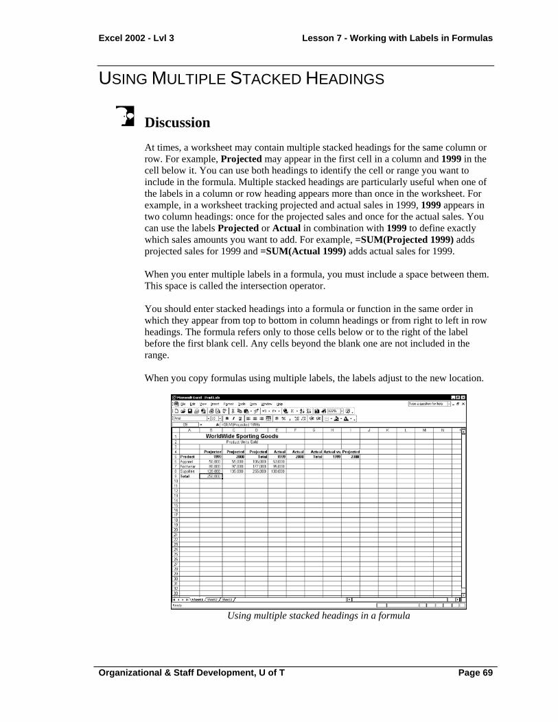
Excel 2002 - Lvl 3 Lesson 7 - Working with Labels in Formulas
Organizational & Staff Development, U of T Page 69
USING MULTIPLE STACKED HEADINGS
Discussion At times, a worksheet may contain multiple stacked headings for the same column or row. For example, Projected may appear in the first cell in a column and 1999 in the cell below it. You can use both headings to identify the cell or range you want to include in the formula. Multiple stacked headings are particularly useful when one of the labels in a column or row heading appears more than once in the worksheet. For example, in a worksheet tracking projected and actual sales in 1999, 1999 appears in two column headings: once for the projected sales and once for the actual sales. You can use the labels Projected or Actual in combination with 1999 to define exactly which sales amounts you want to add. For example, =SUM(Projected 1999) adds projected sales for 1999 and =SUM(Actual 1999) adds actual sales for 1999. When you enter multiple labels in a formula, you must include a space between them. This space is called the intersection operator. You should enter stacked headings into a formula or function in the same order in which they appear from top to bottom in column headings or from right to left in row headings. The formula refers only to those cells below or to the right of the label before the first blank cell. Any cells beyond the blank one are not included in the range. When you copy formulas using multiple labels, the labels adjust to the new location.
Using multiple stacked headings in a formula

Lesson 7 - Working with Labels in Formulas Excel 2002 - Lvl 3
Page 70 Organizational & Staff Development, U of T
Procedures
1. Select the cell in which you want to create the formula.
2. Start typing the formula or function.
3. Type the first column or row heading label.
4. Type a space.
5. Type the second column or row heading label.
6. Type the remainder of the formula as needed.
7. Press [Enter].
REFERRING TO INDIVIDUAL CELLS
Discussion You can use a natural language formula to refer to a single cell in a worksheet. To refer to a single cell, you enter both the column and row headings for that cell. The column and row headings can be entered in any order. For example, in a worksheet containing 1999 sales for different sporting goods products, the formula =1999 Footwear refers to the data in the cell at the intersection of the column heading 1999 and the row heading Footwear. You can also use stacked headings in a label that refers to a single cell. When you copy a formula using a label to refer to a single cell to a new location, the label adjusts accordingly.

Excel 2002 - Lvl 3 Lesson 7 - Working with Labels in Formulas
Organizational & Staff Development, U of T Page 71
Referring to individual cells
Procedures
1. Select the cell in which you want to create the formula.
2. Start typing the formula or function.
3. Type the label defining the first cell reference.
4. Type a space.
5. Type the label defining the second cell reference.
6. Type the remainder of the formula as needed.
7. Press [Enter].

LESSON 8 - CREATING AND EDITING CHARTS
In this lesson, you will learn how to:
• Use charts
• Create charts with the Chart Wizard
• Move and resize charts
• Identify chart objects
• Change the chart type
• Change the chart type and sub-type
• Change the plot direction
• Remove/Add a legend
• Move the legend
• Chart non-adjacent ranges
• Change the chart range
• Change the data source
• Change the chart location
• Print a chart
• Delete a chart

Excel 2002 - Lvl 2 Lesson 8 - Creating and Editing Charts
Organizational & Staff Development, U of T Page 73
USING CHARTS
Discussion A chart uses values in a worksheet to create a graphic representation of their relationship to one another. You can use charts to make it easier to spot trends, highlight important changes, and compare individual figures. For example, when comparing sales amounts, a column chart dramatically illustrates differences between two or more sales amounts. Using charts in reports and presentations displays numbers in a format that is easy to understand. When you create a chart, each row or column of data on the worksheet becomes a data series. Each individual value within the row or column is called a data point. The range you chart can include row and column headings. These headings are used as the category labels and legend text. If the range does not include headings, Excel creates default headings. In Excel, you can either embed a chart in the worksheet, or you can create it on a chart sheet. An embedded chart is a chart object in the worksheet. When you want the chart and the worksheet data viewed or printed together, you should use an embedded chart. A chart sheet is a separate worksheet in the workbook that contains only the chart. If you want to use the chart by itself (for example, in a presentation), you should use a chart sheet. Both types of charts are linked to the worksheet data and update automatically if the data is changed.
A column chart

Lesson 8 - Creating and Editing Charts Excel 2002 - Lvl 2
Page 74 Organizational & Staff Development, U of T
CREATING CHARTS WITH THE CHART WIZARD
Discussion The Chart Wizard assists you in creating a chart by leading you through a series of dialog boxes that allow you to choose options for the chart. You can use the Chart Wizard to quickly learn the essentials of creating a chart. For example, if you have never created a chart to demonstrate monthly sales by representative, the Chart Wizard will guide you through the process. The Chart Wizard contains four steps. In the first step, you select the chart type and sub-type. In the second step, you select or verify the data that will be used to create the chart. The third step allows you to select various chart options. The last step determines whether the chart will be embedded in the worksheet or displayed in its own chart sheet.
A chart created with the Chart Wizard
After you have created a chart, you can edit it to change any chart feature.
You can preview the selected chart type and sub-type by clicking and holding the Press and hold to view sample button in Step 1 of the Chart Wizard.

Excel 2002 - Lvl 2 Lesson 8 - Creating and Editing Charts
Organizational & Staff Development, U of T Page 75
To modify an existing chart, you can access any one of the four Chart Wizard pages by right-clicking the chart you want to edit and selecting the Chart Type, Source Data, Chart Options, or Location command.
Procedures
1. Select the range containing the data you want to chart.
2. Click the Chart Wizard button on the Standard toolbar.
3. Select the desired chart type from the Chart type list box.
4. Select the desired chart sub-type under Chart sub-type.
5. Select Next >.
6. Select the desired Series in option.
7. Select Next >.
8. Select the desired chart options tab.
9. Select the desired chart options.
10. Select Next >.
11. Select the desired chart placement.
12. Select Finish.
MOVING AND RESIZING CHARTS
Discussion After a chart has been placed on a worksheet, it can be moved and resized. You can move a chart to place it in a desired location. For example, if you have created an embedded chart that hides your data, you can move it to a more appropriate location. Resizing a chart allows you to create a larger or smaller chart. For example, you may want to increase the size of a chart so that its labels are more legible.
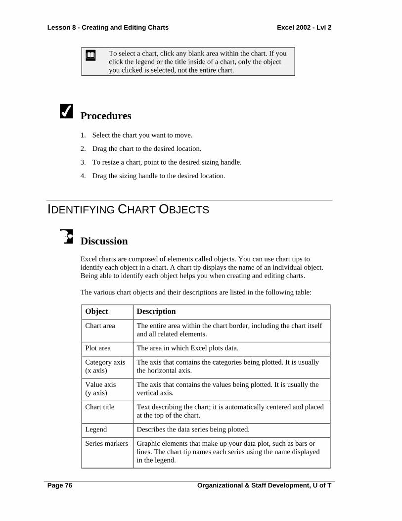
Lesson 8 - Creating and Editing Charts Excel 2002 - Lvl 2
Page 76 Organizational & Staff Development, U of T
To select a chart, click any blank area within the chart. If you click the legend or the title inside of a chart, only the object you clicked is selected, not the entire chart.
Procedures
1. Select the chart you want to move.
2. Drag the chart to the desired location.
3. To resize a chart, point to the desired sizing handle.
4. Drag the sizing handle to the desired location.
IDENTIFYING CHART OBJECTS
Discussion Excel charts are composed of elements called objects. You can use chart tips to identify each object in a chart. A chart tip displays the name of an individual object. Being able to identify each object helps you when creating and editing charts. The various chart objects and their descriptions are listed in the following table:
Object Description
Chart area The entire area within the chart border, including the chart itself and all related elements.
Plot area The area in which Excel plots data.
Category axis (x axis)
The axis that contains the categories being plotted. It is usually the horizontal axis.
Value axis (y axis)
The axis that contains the values being plotted. It is usually the vertical axis.
Chart title Text describing the chart; it is automatically centered and placed at the top of the chart.
Legend Describes the data series being plotted.
Series markers Graphic elements that make up your data plot, such as bars or lines. The chart tip names each series using the name displayed in the legend.

Excel 2002 - Lvl 2 Lesson 8 - Creating and Editing Charts
Organizational & Staff Development, U of T Page 77
Object Description
Data points The individual parts of a data series. Data points can be bars, points on a line, a slice of a pie, a circle, etc. Data points are identified in chart tips by the series name and the value of the data point.
Gridlines Lines that extend from an axis across the plot area to help guide the eye from the data point to its corresponding value.
Not all objects appear in every chart type. For example, pie charts do not have axes.
Viewing a chart tip
If the chart tips are not visible, you can select the Show names option on the Chart page in the Options dialog box.
You can use the Chart Objects list on the Chart toolbar to select any available chart object.
You should be careful when selecting a chart object. For example, it is easy to select the plot area when you are trying to select the category axis. Therefore, when you select a chart object, you should verify that the sizing handles appear around the correct chart object.

Lesson 8 - Creating and Editing Charts Excel 2002 - Lvl 2
Page 78 Organizational & Staff Development, U of T
Procedures
1. Point to any chart object to display its chart tip.
CHANGING THE CHART TYPE
Discussion You can change the chart type to one of a number of types, including column, bar, line, pie, XY (scatter), area, doughnut, radar, surface, bubble, stock, cylinder, cone, and pyramid. Changing the chart type changes the way your data is represented. For example, if your sales data appears in a line chart, it clearly demonstrates sales trends. Using the same data in a pie chart provides a clear picture of what percentage of the total sales each amount represents.
Changing the chart type

Excel 2002 - Lvl 2 Lesson 8 - Creating and Editing Charts
Organizational & Staff Development, U of T Page 79
Procedures
1. Select the chart.
2. Click the arrow on the Chart Type button on the Chart toolbar.
3. Select the desired chart type.
CHANGING THE CHART TYPE AND SUB-TYPE
Discussion You can use the Chart Type dialog box to change the chart type and sub-type. You can select from a number of different chart types. In addition, you can choose from a number of sub-types for each chart type. The sub-types are variations of the main chart type. For example, you can display a bar chart with a stacked, clustered, or 3-D effect.
The Chart Type dialog box
You can also right-click a chart and select the Chart Type command or use the Chart toolbar to change the chart type.

Lesson 8 - Creating and Editing Charts Excel 2002 - Lvl 2
Page 80 Organizational & Staff Development, U of T
You can preview the selected chart type and sub-type by clicking and holding the Press and hold to view sample button in the Chart Type dialog box.
Procedures
1. Select the chart.
2. Select the Chart menu.
3. Select the Chart Type command.
4. Select the desired chart type from the Chart type list box.
5. Select the desired chart sub-type under Chart sub-type.
6. To remove custom formatting and apply the default chart formatting, select the Default formatting option.
7. Select OK.
CHANGING THE PLOT DIRECTION
Discussion You can use the By Row and By Column buttons on the Chart toolbar to change the plot direction of the data. For example, you can change a sales chart that displays the representatives names along the category axis and the month names in the legend to a sales chart that displays the month names along the category axis and the representatives names in the legend. The By Row button changes the chart so that the data series is taken from rows of data. The By Column button changes the chart so that the data series is taken from columns of data.
Procedures
1. Select the chart.
2. To change the plot direction from columns to rows, click the By
Row button on the Chart toolbar.

Excel 2002 - Lvl 2 Lesson 8 - Creating and Editing Charts
Organizational & Staff Development, U of T Page 81
3. To change the plot direction from rows to columns, click the By
Column button on the Chart toolbar.
REMOVING/ADDING A LEGEND
Discussion In a chart, a legend is used to label the data series. When you create a chart with the Chart Wizard, the legend automatically appears. However, you can remove the legend if you want more room in the chart, if you want to make the chart smaller, or if you want to identify the data series in some other way. For example, if you are going to add a data table, the legend is redundant and takes up valuable space on the chart.
A chart without a legend
You can also reposition the legend by selecting it and dragging it to a new location.
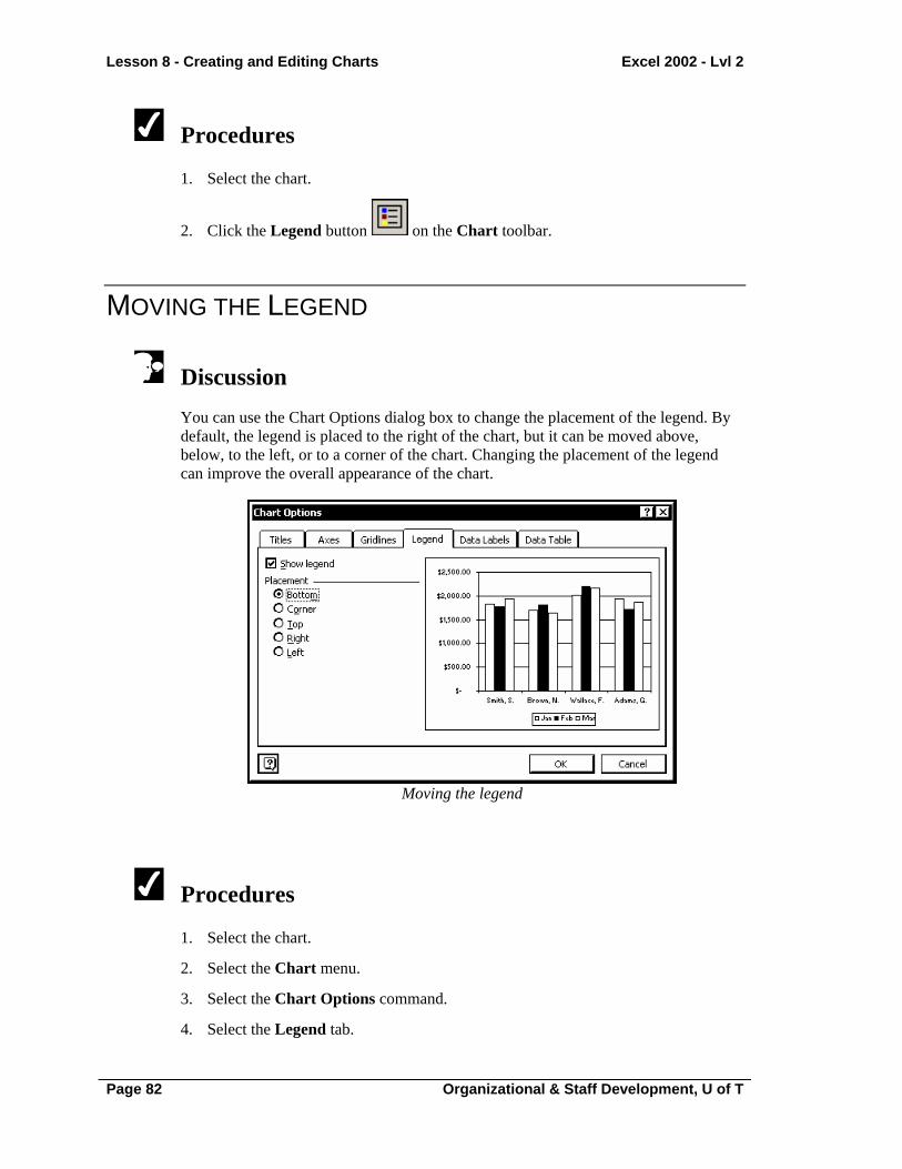
Lesson 8 - Creating and Editing Charts Excel 2002 - Lvl 2
Page 82 Organizational & Staff Development, U of T
Procedures
1. Select the chart.
2. Click the Legend button on the Chart toolbar.
MOVING THE LEGEND
Discussion You can use the Chart Options dialog box to change the placement of the legend. By default, the legend is placed to the right of the chart, but it can be moved above, below, to the left, or to a corner of the chart. Changing the placement of the legend can improve the overall appearance of the chart.
Moving the legend
Procedures
1. Select the chart.
2. Select the Chart menu.
3. Select the Chart Options command.
4. Select the Legend tab.

Excel 2002 - Lvl 2 Lesson 8 - Creating and Editing Charts
Organizational & Staff Development, U of T Page 83
5. Select the Show legend option, if necessary.
6. Select the desired placement option.
7. Select OK.
CHARTING NON-ADJACENT RANGES
Discussion You can chart non-adjacent ranges in a worksheet. This option allows you to select only the data you want to chart and is especially useful when you want to plot only one data series, as in a pie chart.
Charting non-adjacent ranges
Procedures
1. Select the first range you want to chart.
2. Hold [Ctrl] and select the non-adjacent range(s).
3. Click the Chart Wizard button on the Standard toolbar.
4. Select the Standard Types tab.

Lesson 8 - Creating and Editing Charts Excel 2002 - Lvl 2
Page 84 Organizational & Staff Development, U of T
5. Select the desired chart type from the Chart type list box.
6. Select the desired chart sub-type under Chart sub-type.
7. Select Next >.
8. Select the desired Rows or Columns series option, if necessary.
9. Select Next >.
10. Select the desired chart options tab.
11. Select the desired chart options.
12. Select Next >.
13. Select the desired chart placement.
14. Select Finish.
CHANGING THE CHART RANGE
Discussion When a chart is selected, colored borders appear around the labels and data used in the chart. You can add or remove data from a chart by changing the border surrounding the data to include or exclude one or more series of data. For example, if you want to remove a sales representative from a chart, you can drag the border surrounding the sales data so that it does not include that representative. You can only redefine the range to include or exclude adjacent data.
If the chart is on a separate chart sheet, you can use the Source Data dialog box to change the data range. You can change a data range by right-clicking the chart, selecting the Source Data command, and selecting the Data Range page. Then, enter the new range into the Data range box.
Procedures
1. Select the chart.
2. Point to the fill handle in the border surrounding the data used in the chart.
3. Drag the fill handle to include or exclude data as desired.
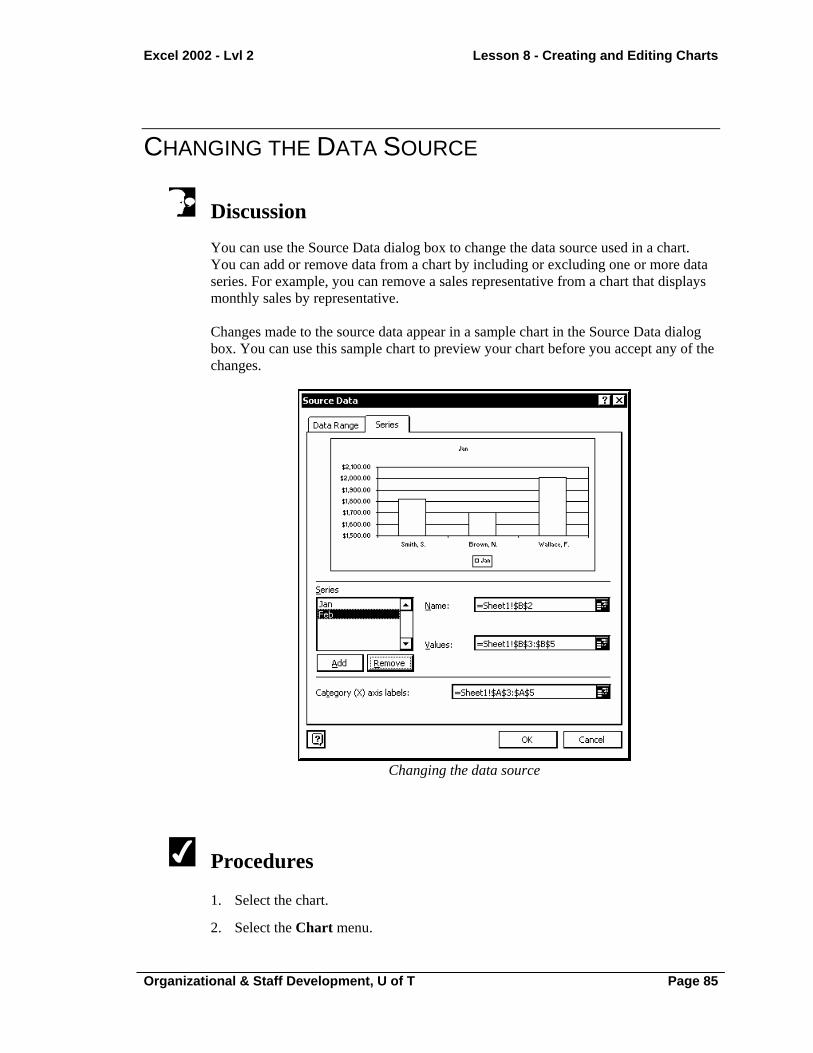
Excel 2002 - Lvl 2 Lesson 8 - Creating and Editing Charts
Organizational & Staff Development, U of T Page 85
CHANGING THE DATA SOURCE
Discussion You can use the Source Data dialog box to change the data source used in a chart. You can add or remove data from a chart by including or excluding one or more data series. For example, you can remove a sales representative from a chart that displays monthly sales by representative. Changes made to the source data appear in a sample chart in the Source Data dialog box. You can use this sample chart to preview your chart before you accept any of the changes.
Changing the data source
Procedures
1. Select the chart.
2. Select the Chart menu.

Lesson 8 - Creating and Editing Charts Excel 2002 - Lvl 2
Page 86 Organizational & Staff Development, U of T
3. Select the Source Data command.
4. Select the Series tab.
5. Select the data series you want to remove from the Series list box.
6. Select Remove.
7. Select OK.
CHANGING THE CHART LOCATION
Discussion You can use the Chart Location dialog box to change the location of a chart. The chart can be placed on an existing worksheet or in its own chart sheet. For example, you may want to use the worksheet without the chart. Placing the chart on a chart sheet retains the chart as part of the file, but removes it from the worksheet. Chart sheets are inserted to the left of the worksheet containing the data represented by the chart. Charts on chart sheets are still linked to the data in the worksheets and update automatically whenever the data changes.
Procedures
1. Select the chart.
2. Select the Chart menu.
3. Select the Location command.
4. Select the As new sheet option.
5. Select OK.
PRINTING A CHART
Discussion Charts embedded in a worksheet print automatically when you print the worksheet. If you want to print just the chart, you can select it before you print. For example, you may want to print the chart to use as a slide overhead for a presentation.

Excel 2002 - Lvl 2 Lesson 8 - Creating and Editing Charts
Organizational & Staff Development, U of T Page 87
You can also print a chart from the Print dialog box. When a chart is selected, the Selection option in the Print dialog box changes to Selected Chart.
You can also print a chart sheet by first selecting it and then clicking the Print button.
Procedures
1. To print the chart without the worksheet data, select the chart.
2. Click the Print button .
3. To print the chart with the worksheet data, click outside the chart in the worksheet area.
4. Click the Print button .
DELETING A CHART
Discussion If you no longer need a chart, you can delete it from the worksheet. When you delete a chart, only the chart is deleted; the data from which the chart was created remains in the worksheet.
You can delete a chart sheet by right-clicking the desired chart sheet tab, selecting the Delete command, and then selecting Delete.
Procedures
1. Select the chart you want to delete.
2. Press [Delete].

LESSON 9 - FORMATTING CHARTS
In this lesson, you will learn how to:
• Format charts
• Add chart titles
• Format chart objects
• Change the text orientation

Excel 2002 - Lvl 2 Lesson 9 - Formatting Charts
Organizational & Staff Development, U of T Page 89
FORMATTING CHARTS
Discussion You can edit an existing chart to improve its appearance and modify how data is charted. You can use the Chart Options dialog box to add or hide chart objects. You can add titles to the chart, display or hide the chart axes and/or axis gridlines, position the legend, and add data labels and/or a data table. Each object in a chart can be formatted. The formatting options vary, depending upon the chart object selected. Chart objects can be formatted using either the Format dialog box for the corresponding chart object or the Formatting toolbar. For example, you can change the appearance of the text in the chart title by opening the Format Chart Title dialog box or by using the buttons the Formatting toolbar.
ADDING CHART TITLES
Discussion You can use the Chart Options dialog box to add titles to a chart. You can add a chart title that is centered at the top of a chart and identifies the basic information conveyed in the chart. In addition, you can add titles to the chart axes. Each axis title will appear along the corresponding axis. For example, you may want to add a title to the value axis, indicating the scale of the numbers represented (e.g., thousands).

Lesson 9 - Formatting Charts Excel 2002 - Lvl 2
Page 90 Organizational & Staff Development, U of T
Adding chart titles
Procedures
1. Select the chart.
2. Select the Chart menu.
3. Select the Chart Options command.
4. Select the Titles tab.
5. Select the desired title box.
6. Type the desired title text.
7. Select OK.
FORMATTING CHART OBJECTS
Discussion You can use the Format button on the Chart toolbar to format a selected chart object. Formatting changes the appearance of the chart. For example, if you are using the chart in a presentation, you may want to change the font of the chart text to match the font used throughout the presentation. The formatting options available depend on the selected object. For example, if the chart area is selected, you can change the patterns, fonts, and chart area properties. If the category axis is selected, you can change the patterns, scale, font, number, and

Excel 2002 - Lvl 2 Lesson 9 - Formatting Charts
Organizational & Staff Development, U of T Page 91
alignment. You can click to select the desired chart object, or you can select it from the Chart Objects list on the Chart toolbar. You can also use the buttons on the Formatting toolbar to format text and values, as well as data point and data series fill colors and patterns.
The name of the Format button changes depending on the object selected. For example, if the chart area is selected, the button name changes to Format Chart Area. If the category axis is selected, the button name changes to Format Axis.
You can also double-click a chart object to open the corresponding Format dialog box.
Clicking a series object (such as a column in a column chart) selects the entire series. The Format button then opens the Format Data Series dialog box and any changes are applied to all the objects in the series. However, clicking a series object a second time selects only that data point. The Format button then opens the Format Data Point dialog box and any changes are applied only to that single object.
Procedures
1. Select the chart object you want to format.
2. Click the Format button on the Chart toolbar.
3. Select the desired tab.
4. Make the desired changes.
5. Select OK.
CHANGING THE TEXT ORIENTATION
Discussion You can use the Angle Clockwise or Angle Counterclockwise buttons on the Chart toolbar to change the orientation of selected text in a chart. The Angle Clockwise button angles selected text downward at a 45-degree angle. The text is angled so that the first letter appears at the top and the last letter at the bottom. The Angle

Lesson 9 - Formatting Charts Excel 2002 - Lvl 2
Page 92 Organizational & Staff Development, U of T
Counterclockwise button angles selected text upward at a 45-degree angle. The text is angled so that the first letter appears at the bottom and the last letter at the top. You can angle text to provide room for long labels on the category axis or to improve the appearance of the chart. For example, if a chart contains multiple entries for sales representatives along the category axis, you can angle the labels to make them easier to read.
If the text is already angled, clicking the Angle Clockwise or Angle Counterclockwise button returns the text to its default alignment.
Procedures
1. Select the text you want to angle.
2. To angle the text downward, click the Angle Clockwise button on the Chart toolbar.
3. To angle the text upward, click the Angle Counterclockwise button
on the Chart toolbar.
LESSON 10 - DRAWING AN OBJECT
In this lesson, you will learn how to:
• Work with drawing objects
• Draw enclosed objects
• Draw a line
• Select filled and unfilled objects
• Move an object
• Add text to an object
• Select text in an object
• Resize an object
• Format lines
• Change and remove the fill color
• Change the font color
• Delete an object

Lesson 10 - Drawing an Object Excel 2002 - Lvl 2
Page 94 Organizational & Staff Development, U of T
WORKING WITH DRAWING OBJECTS
Discussion A drawing object is a rectangle, oval, line, arrow, or polygon that is drawn directly on a worksheet to enhance it. For example, arrows can be used to point to important data, rectangles or ovals can be used to draw attention to specific areas of a worksheet, and lines can be used to divide different areas of a worksheet. Drawing objects can also be used to draw attention to trends or growth spurts in charts. Drawing objects float on top of cells and can be moved or copied to any location on a worksheet. Once drawn, objects can be modified to change their shape, size, color, fill, and pattern, as well as a number of other attributes. The Drawing toolbar enables you to create lines, lines with arrows, rectangles, and ovals. You can also select various AutoShapes from a number of categories, including Connectors, Basic Shapes, Block Arrows, Flowcharts, Stars and Banners, and Callouts. The Drawing toolbar provides buttons that allow you to make adjustments to fill and font colors, as well as line, dash, and arrow styles. You can also add shadow effects to an object and enter text into objects.
The Drawing button acts as a toggle to display or hide the Drawing toolbar.
You can also display the Drawing toolbar by right-clicking the menu bar or any toolbar and selecting the Drawing command.
DRAWING ENCLOSED OBJECTS
Discussion The drawing tools on the Drawing toolbar allow you to draw objects directly onto a worksheet. You can draw enclosed objects and then move, copy, and/or resize them as desired. Enclosed drawing objects (such as rectangles or ovals) are filled by default. Filled objects are opaque and contain patterns and/or colors. If filled objects are drawn in front of data in a worksheet, the data is hidden. You can, however, remove an object’s fill. Unfilled objects allow any data in the cells behind them to be seen.

Excel 2002 - Lvl 2 Lesson 10 - Drawing an Object
Organizational & Staff Development, U of T Page 95
Rectangles, unlike cell borders, can be drawn in the middle of cells. A filled rectangle can be used to hide sensitive data. For example, if you are making a presentation, a rectangle can be placed over salary information. When you are drawing an object, the mouse pointer changes into a crosshair. The center of the crosshair represents the outer border of the object.
To draw a square or a circle, click either the Rectangle button or the Oval button respectively and hold the [Shift] key as you drag.
To insert a drawing object with a predefined size, click the applicable drawing object button and then click in the desired area of the worksheet.
To draw more than one object of the same type, double-click the applicable drawing object button. After you have drawn the desired number of objects, you can press the [Esc] key or click the applicable drawing object button again to return to normal editing mode.
Procedures
1. Click the Drawing button on the Standard toolbar.
2. Click the applicable drawing object button on the Drawing toolbar.
3. Drag to position and size the object as desired.
DRAWING A LINE
Discussion Lines can be used to indicate separate sections of a worksheet. For example, you can add a line to separate a heading from data in a worksheet. Lines can be drawn at various angles and positions. Drawn lines, as opposed to cell borders, can be drawn in the middle of cells and can also be moved and sized as desired. When you draw a line, the mouse pointer changes into a crosshair. The center of the crosshair is the point at which the line is drawn.

Lesson 10 - Drawing an Object Excel 2002 - Lvl 2
Page 96 Organizational & Staff Development, U of T
To draw a straight line, hold the [Shift] key as you drag. If you move the mouse pointer up or down, the angle of the line will change in 15-degree increments.
Procedures
1. Click the Line button on the Drawing toolbar.
2. Drag from the beginning to the end point of the line.
SELECTING FILLED AND UNFILLED OBJECTS
Discussion Before you can modify a drawing object, you must select it. When an object is selected, white sizing handles appear around it. Any formatting commands you perform affect only the selected object. An object remains selected until you select another object or click elsewhere in the worksheet area. Different methods are used to select filled and unfilled objects. Since an unfilled object is empty, you must click its border in order to select it. You can, however, click anywhere in a filled object to select it. In addition, if an object contains text, you must click the border to select the object itself in order to perform certain tasks, such as changing the fill or font color.

Excel 2002 - Lvl 2 Lesson 10 - Drawing an Object
Organizational & Staff Development, U of T Page 97
Selecting an unfilled object
To select more than one drawing object, click the Select Objects button on the Drawing toolbar and drag to select all adjacent objects, or hold the [Shift] key and click each object you want to select.
Procedures
1. Click in any filled object to select it.
2. Click the border of any unfilled object to select it.
MOVING AN OBJECT
Discussion After you have created an object, you can move it to a different area of the worksheet by dragging it to the desired location. For example, you may have an object positioned at the top left of the worksheet and then decide you would rather have a heading appear there instead. You can select the object and move it to a different area. The mouse pointer must be a single, white arrow with a black, four-headed arrow attached to it to move a graphic.

Lesson 10 - Drawing an Object Excel 2002 - Lvl 2
Page 98 Organizational & Staff Development, U of T
You can use the keyboard when you want to move an object in small increments. Select the object and press the arrow key on the keyboard that corresponds to the direction in which you want to move the object.
Procedures
1. Drag the object you want to move to the desired location.
ADDING TEXT TO AN OBJECT
Discussion You can add text to an enclosed object. If you combine text with an object, you can create logos or banners to accentuate your worksheet. For example, you can use text within an object to create your company logo on a marketing worksheet. Text in an object wraps within the object’s borders.
Adding text to an object

Excel 2002 - Lvl 2 Lesson 10 - Drawing an Object
Organizational & Staff Development, U of T Page 99
Procedures
1. Select the object to which you want to add text.
2. Type the desired text.
3. To add an additional line of text, press [Enter].
4. Type additional text as desired.
5. When you have finished adding the desired text, click anywhere in the worksheet area to deselect the object.
SELECTING TEXT IN AN OBJECT
Discussion When an object contains text, clicking within the object places the insertion point in the text. You can then edit, select, or format the text. For example, after creating a logo, you may want to change the font and style of its text. However, if you click the object’s border, the object itself is selected and the insertion point does not appear. In this case, any changes you make will affect all the text in the object. To format specific text in an object, you must select the text you want to change.
When text is selected, the selection border around the object is composed of slashes. When the object itself is selected, the selection border around it is composed of dots.
When selecting text, make sure that the mouse pointer does not appear as a single, white arrow with a black, four-headed arrow attached to it. This mouse pointer indicates the movement of objects, not the selection of text.
Procedures
1. Select an object that contains text.
2. To place the insertion point within the text, click in the object.
3. Drag to select the desired text within the object.

Lesson 10 - Drawing an Object Excel 2002 - Lvl 2
Page 100 Organizational & Staff Development, U of T
RESIZING AN OBJECT
Discussion You may want to resize an object so that it fits better in the worksheet. Drawing objects can easily be resized using their sizing handles. If you drag a middle sizing handle on the side of any object, you change the size in that one direction only. If you drag any sizing handle at the corner of an object, however, you change the size in two directions at once.
When text within an object is selected, the object border is composed of slashes. When the object itself is selected, its border is composed of dots.
Procedures
1. Select the object you want to resize.
2. Drag any sizing handle as desired to increase or decrease the size of the object.
FORMATTING LINES
Discussion You can format lines by changing the line style, color, and dash style. In an enclosed object, the line is the border around an object. In an open object, such as a line or an arrow, the line is the object itself. You can change the style of any existing line. Line styles can be used to change the thickness of a line or to create double and triple lines. For example, to dramatically separate a heading from data in a worksheet, you can increase the width of the line that separates them. In addition, you can change an existing line to a dash style. Dash styles break the line into dots or dashes. Dashed lines can help to enhance the appearance of a worksheet or to identify a means of separation.

Excel 2002 - Lvl 2 Lesson 10 - Drawing an Object
Organizational & Staff Development, U of T Page 101
You can also change the line color of a drawing object. Changing the line color can enhance the appearance of the object. For example, if you are creating a logo, changing the line color can help distinguish the border of the logo. The Line Color button has two components. The Line Color button displays the currently selected color. To apply the currently selected color to another object, you only have to select the object and click the Line Color button. In addition, you can use the Line Color list to select a different color from the color palette.
Formatting a line
Procedures
1. Select the object containing the line you want to format.
2. To change the line style, click the Line Style button on the Drawing toolbar.
3. Select the desired line style.
4. To change the dash style, click the Dash Style button on the Drawing toolbar.
5. Select the desired dash style.
6. To change the line color, click the arrow on the Line Color button
on the Drawing toolbar.

Lesson 10 - Drawing an Object Excel 2002 - Lvl 2
Page 102 Organizational & Staff Development, U of T
7. Select the desired line color.
CHANGING AND REMOVING THE FILL COLOR
Discussion You can change the fill color of an object at any time. Changing the fill color enhances the appearance of objects. If a rectangle contains text, filling the rectangle with a bright color highlights the text. An unfilled object can be used to call attention to a cell or range in a worksheet. For example, you can use an oval to circle particularly high or low sales values in a worksheet. Enclosed objects, however, are filled by default and are opaque. You must select the No Fill option to remove the fill and make an object transparent. An unfilled object reveals the cells behind it. The Fill Color button has two components. The Fill Color button displays the currently selected color. To apply the currently selected color to another object, you only have to select the object and click the Fill Color button. You can also use the Fill Color list to select the desired color from the color palette.
Changing the fill color of an object
When text within an object is selected, the object border is composed of slashes. When the object itself is selected, its border is composed of dots.

Excel 2002 - Lvl 2 Lesson 10 - Drawing an Object
Organizational & Staff Development, U of T Page 103
The Fill Color button is also located on the Formatting toolbar.
Procedures
1. Select the object containing the fill color you want to change.
2. Click the arrow on the Fill Color button on the Drawing toolbar.
3. Select the desired fill color.
CHANGING THE FONT COLOR
Discussion You can change the color of the font in any object that contains text. You can change the color of all the text in the object, or you can change only the font color of selected characters. Changing font color draws attention to text. When selecting a font color for text, you should be aware of the background color of the object. For example, red text will stand out on a white background, whereas yellow text will not. The Font Color button has two components. The Font Color button displays the currently selected color. To apply the currently selected color to another object, you only have to select the object and click the Font Color button. In addition, you can use the Font Color list to select a different color from color palette.
When text within an object is selected, the object border is composed of slashes. When the object itself is selected, its border is composed of dots.
The Font Color button is also located on the Formatting toolbar.

Lesson 10 - Drawing an Object Excel 2002 - Lvl 2
Page 104 Organizational & Staff Development, U of T
Procedures
1. Select the object containing the text with the font color you want to change.
2. Click the arrow on the Font Color button on the Drawing toolbar.
3. Select the desired font color.
DELETING AN OBJECT
Discussion You can delete an object from a worksheet if you no longer need it. If you delete an object accidentally, you can use the Undo feature to restore it to the worksheet.
Procedures
1. Select the object you want to delete.
2. Press [Delete].
LESSON 11 - USING ADDITIONAL EFFECTS AND OBJECTS
In this lesson, you will learn how to:
• Add a 3-D effect
• Apply a 3-D setting
• Add a shadow
• Draw a text box
• Draw an arrow
• Insert pictures
• Format graphics

Lesson 11 - Using Additional Effects and Objects Excel 2002 - Lvl 2
Page 106 Organizational & Staff Development, U of T
ADDING A 3-D EFFECT
Discussion If you want an object to appear three-dimensional, you can add a 3-D effect. For example, if you are creating a logo, a 3-D effect makes the object stand out from the page. You can select from a variety of different 3-D styles.
An object with a 3-D effect
An object can have either a shadow or a 3-D effect, but not both.
You cannot assign a line color to a filled, 3-D object, but you can change the fill color.
Procedures
1. Select the object to which you want to add a 3-D effect.
2. Click the 3-D Style button on the Drawing toolbar.
3. Select the desired 3-D style.

Excel 2002 - Lvl 2 Lesson 11 - Using Additional Effects and Objects
Organizational & Staff Development, U of T Page 107
APPLYING A 3-D SETTING
Discussion Once you have added a 3-D effect to an object, you can apply various depth, direction, lighting, surface, and color settings. You can also tilt 3-D objects down, up, left, or right. Depending on the object selected, certain options may not be available.
If you apply 3-D settings to a selected object without having selected a 3-D style, certain options will have no effect.
Procedures
1. Select the object to which you want to apply a 3-D setting.
2. Click the 3-D Style button on the Drawing toolbar.
3. Select 3-D Settings.
4. Select the desired 3-D setting.
5. Select the desired option, if necessary.
ADDING A SHADOW
Discussion Shadow effects can enhance an object’s appearance. A shadow is a dark border around one or more sides of an object. The shadow makes the object appear raised from the background. For example, a shadow gives the effect of depth to a logo on a worksheet. You can select from a variety of shadows. Once you have added a shadow effect to an object, you can use the Shadow Settings toolbar, available from the Shadow Style list, to modify the shadow effect. From this toolbar, you can move the shadow up, down, right, or left, as well as change the color of the shadow.

Lesson 11 - Using Additional Effects and Objects Excel 2002 - Lvl 2
Page 108 Organizational & Staff Development, U of T
An object can have either a shadow or a 3-D effect, but not both.
Procedures
1. Select the object to which you want to add a shadow.
2. Click the Shadow Style button on the Drawing toolbar.
3. Select the desired shadow style.
DRAWING A TEXT BOX
Discussion A text box is an object specifically designed to contain text. Immediately after drawing a text box, the insertion point appears within the text box. You can type text directly into the text box. Text boxes can be used to add notes, comments, and addendum to a worksheet or chart. A text box allows text to wrap within its borders. Like other drawing objects, a text box floats above the cells in a worksheet. This feature allows you to position the text box anywhere in the worksheet, rather than being constricted to the fixed location of a cell. When you are drawing a text box, the mouse pointer changes into a crosshair. The center of the crosshair is the point at which the lines are drawn.

Excel 2002 - Lvl 2 Lesson 11 - Using Additional Effects and Objects
Organizational & Staff Development, U of T Page 109
A drawn text box
To insert a text box that automatically resizes as you add text, click the Text Box button, click in the desired area of the worksheet, and type the text. The text box automatically resizes horizontally as you type and vertically when you press the [Enter] key.
To edit text in a text box, use the same techniques you would use to edit text in a cell. Once the text box has been selected, position the insertion point and insert or delete text as desired.
Procedures
1. Click the Text Box button on the Drawing toolbar.
2. Drag to draw the text box in the desired size and location.
3. Type the desired text.
4. Click anywhere in the worksheet to deselect the text box.

Lesson 11 - Using Additional Effects and Objects Excel 2002 - Lvl 2
Page 110 Organizational & Staff Development, U of T
DRAWING AN ARROW
Discussion You can use arrows to draw attention to cells or sections in a worksheet. For example, you can use an arrow to point to the highest sales value in a sales worksheet. You can also move and resize arrows as desired. When you draw an arrow, the mouse pointer changes into a crosshair. The center of the crosshair is the point at which the arrow is drawn.
Hold the [Shift] key as you drag to create a straight arrow; the angle of the arrow can be adjusted in 15-degree increments.
When you draw an arrow, the arrow is drawn from the tail to the head. You can use the Arrow Style button on the Drawing toolbar to change the direction of the arrow, as well as the arrowhead style.
Procedures
1. Click the Arrow button on the Drawing toolbar.
2. Drag to draw the arrow in the desired size and location.
INSERTING PICTURES
Discussion Besides adding drawing objects to a worksheet, you can include pictures by inserting graphic images from an existing graphic file. Pictures can include scanned images, photographs, and drawn objects saved as files. Before inserting a graphic image, you can preview it to verify that it is the one you want. Excel accepts several types of graphic file formats. Some formats are accepted without a graphic filter. These formats include .wmf, .emf, .bmp, .rle, .dib, .gif, .jpg, and .png. Other formats require a graphics filter, which can be installed using Office Setup.

Excel 2002 - Lvl 2 Lesson 11 - Using Additional Effects and Objects
Organizational & Staff Development, U of T Page 111
The Picture toolbar appears as soon as you select a picture and disappears when you deselect the picture.
Inserting a picture
If the Picture toolbar does not appear when a picture is selected, you can display it by right-clicking any toolbar and selecting the Picture command.
Clip art can be inserted using the Insert Clip Art task pane, which can be opened by clicking the Insert Clip Art button on the Drawing toolbar or by selecting the Insert menu, the Picture command, and then the Clip Art command. You can search for clip art by keywords, or you can access the Microsoft Clip Organizer and browse through categories of clip art.
By default, the Insert Picture dialog box displays graphic files in Thumbnail view. Since a thumbnail is a miniature representation of the picture, you can easily select the picture you want to insert.
Procedures
1. Select the cell where you want the picture to appear.
2. Click the Insert Picture button on the Drawing toolbar.
Lesson 11 - Using Additional Effects and Objects Excel 2002 - Lvl 2
Page 112 Organizational & Staff Development, U of T
3. Select the Look in list.
4. Select the drive containing the desired graphic file.
5. Open the folder containing the desired graphic file.
6. Select the name of the graphic file you want to insert.
7. Select Insert.
FORMATTING GRAPHICS
Discussion Although graphics (such as drawing objects and pictures) appear with default settings, you can use the Format dialog box to change many of those settings. The name of the Format dialog box corresponds to the selected graphic object; the Format Picture dialog box opens when the selected object is a picture and the Format AutoShape dialog box opens for a selected drawing object. In addition, the options available in the Format dialog box depend upon the type of object selected. When dealing with pictures, you can modify the background color of the picture or place a border around it. Using brightness and contrast controls, you can soften a picture. If you place a picture within a cell or within several merged cells, you can specify if the picture should move and size with the cell. Both drawing objects and pictures can be sized to a specific size or scaled proportionally or non-proportionally. When you scale an object, you resize it to a percentage of its original size. For example, when you resize an object’s width from 100% to 50%, you decrease the width of the object by 50%.

Excel 2002 - Lvl 2 Lesson 11 - Using Additional Effects and Objects
Organizational & Staff Development, U of T Page 113
Formatting a graphic
The Picture toolbar provides buttons for many of the formatting options in the Format Picture dialog box.
The Lock aspect ratio option on the Size page in the Format dialog box allows you to maintain the ratio between a selected object’s height and width whenever you resize it.
You can move a picture by dragging it. You can also resize a picture using any of the sizing handles that appear around a selected picture.
Procedures
1. Right-click the graphic you want to format.
2. Select the Format Picture or Format AutoShape command, as applicable.
3. Select the desired tab.
4 Select the desired options.
5. Select OK.

LESSON 12 - USING AUTOSHAPES AND DIAGRAMS
In this lesson, you will learn how to:
• Work with AutoShapes
• Draw a callout
• Draw a basic shape
• Draw a connector
• Draw a flowchart shape
• Draw a block arrow
• Insert a diagram
• Work with diagrams

Excel 2002 - Lvl 2 Lesson 12 - Using AutoShapes and Diagrams
Organizational & Staff Development, U of T Page 115
WORKING WITH AUTOSHAPES
Discussion All drawn objects are called AutoShapes. In addition to the rectangle, oval, text box, line, and arrow found on the Drawing toolbar, Excel offers a wide variety of additional AutoShapes. These AutoShapes are found on the AutoShapes menu on the Drawing toolbar. There are seven categories of AutoShapes: Lines, Connectors, Basic Shapes, Block Arrows, Flowchart, Stars and Banners, and Callouts. You can use these shapes to further enhance your worksheet. For example, you can use a banner with text as the title of a worksheet. For additional AutoShapes, you can select the More AutoShapes command on the AutoShapes menu to open the Insert Clip Art task pane. From the Insert Clip Art task pane, you can open the Microsoft Clip Organizer, which provides numerous categories of AutoShapes and clip art that can be inserted into a worksheet. You can change the fill color and line color of all AutoShapes. In addition, you can add text to all enclosed AutoShapes. Once you have selected the desired AutoShape, you can drag in the worksheet to define the desired shape and size. Each AutoShape has a default size as well. To insert an AutoShape in its default size, select the desired AutoShape and click in the worksheet. You can also change the size of the AutoShape after inserting it.
Although gridlines are useful as a guide for drawing shapes, you may want to disable them when you print the worksheet. You can disable gridlines by selecting the Tools menu, the Options command, and the View tab. Then, deselect the Gridlines option under Window options.
DRAWING A CALLOUT
Discussion Callouts are used to add comments to cells, charts, or other sections of a worksheet. For example, you can use a callout to comment on a trend in a chart. You can choose from a number of different callout shapes. Callouts include a point that connects the callout to the item on which it is commenting. This point is anchored. When you select the callout, the anchor is visible. You can drag the anchor to move the point.
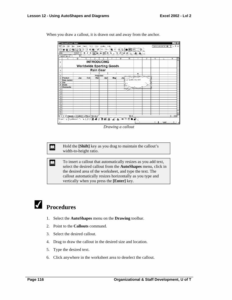
Lesson 12 - Using AutoShapes and Diagrams Excel 2002 - Lvl 2
Page 116 Organizational & Staff Development, U of T
When you draw a callout, it is drawn out and away from the anchor.
Drawing a callout
Hold the [Shift] key as you drag to maintain the callout’s width-to-height ratio.
To insert a callout that automatically resizes as you add text, select the desired callout from the AutoShapes menu, click in the desired area of the worksheet, and type the text. The callout automatically resizes horizontally as you type and vertically when you press the [Enter] key.
Procedures
1. Select the AutoShapes menu on the Drawing toolbar.
2. Point to the Callouts command.
3. Select the desired callout.
4. Drag to draw the callout in the desired size and location.
5. Type the desired text.
6. Click anywhere in the worksheet area to deselect the callout.

Excel 2002 - Lvl 2 Lesson 12 - Using AutoShapes and Diagrams
Organizational & Staff Development, U of T Page 117
DRAWING A BASIC SHAPE
Discussion Basic shapes include a number of different shapes you can use to enhance a worksheet. For example, you can draw a lightning bolt to indicate an electrifying stock performance on a stock worksheet.
Drawing a basic shape
Hold the [Shift] key as you drag to maintain the basic shape’s width-to-height ratio.
Procedures
1. Select the AutoShapes menu on the Drawing toolbar.
2. Point to the Basic Shapes command.
3. Select the desired basic shape.
4. Drag to draw the basic shape in the desired size and location.

Lesson 12 - Using AutoShapes and Diagrams Excel 2002 - Lvl 2
Page 118 Organizational & Staff Development, U of T
DRAWING A CONNECTOR
Discussion Connectors are lines between points on two shapes. Unlike a standard line, a connector is drawn from a point on one shape to a point on another and links the shapes together. As you move connected shapes, the connector lines maintain their link. The points available to connect depend on the shapes involved. Connectors are useful when creating flow diagrams or organization charts. For example, you can use a connector to connect two rectangles indicating different departments in a company organization chart.
Drawing a connector
Procedures
1. Select the AutoShapes menu on the Drawing toolbar.
2. Point to the Connectors command.
3. Select the desired connector.
4. Point to the first shape you want to connect.
5. Click the desired point on the shape.
6. Point to the second shape you want to connect.

Excel 2002 - Lvl 2 Lesson 12 - Using AutoShapes and Diagrams
Organizational & Staff Development, U of T Page 119
7. Click the desired point on the shape.
DRAWING A FLOWCHART SHAPE
Discussion Flowchart shapes indicate specific actions or connections in a flowchart. For example, one shape can indicate a decision, and another a process. Flowchart shapes can be used to create diagrams for decision-making, technical flowcharts, and programming charts.
Drawing a flowchart shape
Hold the [Shift] key as you drag to maintain the flowchart shape’s width to height ratio.
To determine a flowchart shape’s function, you can point to the desired flowchart shape on the Flowchart submenu. The flowchart shape’s function will then appear in a ScreenTip (e.g., Flowchart: Decision).

Lesson 12 - Using AutoShapes and Diagrams Excel 2002 - Lvl 2
Page 120 Organizational & Staff Development, U of T
Procedures
1. Select the AutoShapes menu on the Drawing toolbar.
2. Point to the Flowchart command.
3. Select the desired flowchart shape.
4. Drag to draw the flowchart in the desired size and location.
DRAWING A BLOCK ARROW
Discussion Block arrows are enclosed arrows that can be used to indicate multiple directions. For example, you can use a block arrow to indicate the alternate paths a reader should follow when examining what-if scenarios in a worksheet.
Drawing a block arrow
Hold the [Shift] key as you drag to maintain the shape’s width to height ratio.
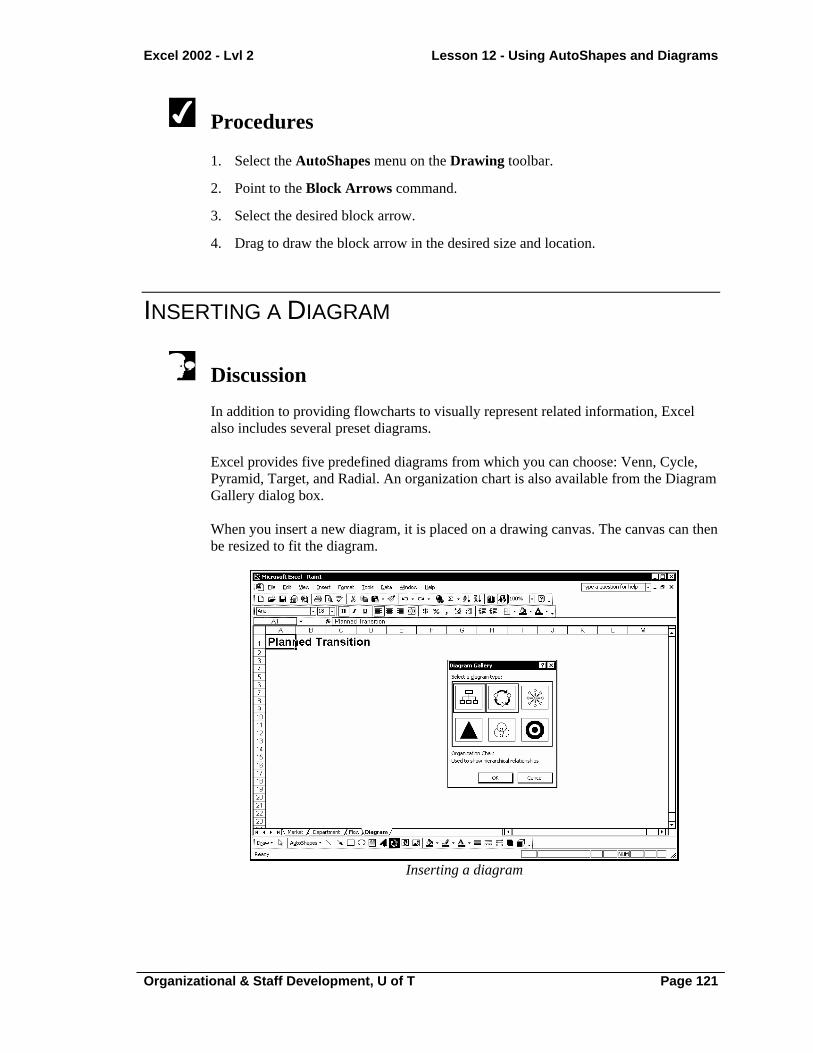
Excel 2002 - Lvl 2 Lesson 12 - Using AutoShapes and Diagrams
Organizational & Staff Development, U of T Page 121
Procedures
1. Select the AutoShapes menu on the Drawing toolbar.
2. Point to the Block Arrows command.
3. Select the desired block arrow.
4. Drag to draw the block arrow in the desired size and location.
INSERTING A DIAGRAM
Discussion In addition to providing flowcharts to visually represent related information, Excel also includes several preset diagrams. Excel provides five predefined diagrams from which you can choose: Venn, Cycle, Pyramid, Target, and Radial. An organization chart is also available from the Diagram Gallery dialog box. When you insert a new diagram, it is placed on a drawing canvas. The canvas can then be resized to fit the diagram.
Inserting a diagram

Lesson 12 - Using AutoShapes and Diagrams Excel 2002 - Lvl 2
Page 122 Organizational & Staff Development, U of T
If you have already created a diagram and want to change its type, you can select the Change to list on the Diagram toolbar and select another diagram type.
You can resize the drawing canvas by dragging one of the black sizing handles.
Procedures
1. Click the Insert Diagram or Organization Chart button on the Drawing toolbar.
2. Select the desired diagram type.
3. Select OK.
WORKING WITH DIAGRAMS
Discussion You can customize a diagram to meet your needs. Additional shapes can be inserted and moved from front to back, labels can be added, and the shapes within the diagram can be changed to different colors and/or styles to emphasize distinct concepts. Excel provides an AutoFormat feature that allows you to pick from predefined styles. You can, however, disable this feature and work on your own. Diagram layout options include tightly fitting the drawing canvas to the diagram, expanding the drawing canvas to add more white space around the diagram, and scaling the diagram to resize it. To freely move diagram elements, you must disable the AutoLayout feature. Even after your diagram has been created, you can change to another diagram type by selecting the Change to button on the Diagram toolbar. When changing diagram types, Excel enables both the AutoLayout and AutoFormat features.

Excel 2002 - Lvl 2 Lesson 12 - Using AutoShapes and Diagrams
Organizational & Staff Development, U of T Page 123
Working with diagrams
The Cycle, Venn, and Target diagrams provide text boxes for each shape. The text boxes can be resized if the AutoLayout feature is disabled.
You can also resize a diagram by double-clicking in a blank area of the drawing canvas and using the Size page in the Format Diagram dialog box to size or scale the diagram.
You can change the format of the shape to which an AutoFormat style has been applied by right-clicking the shape and deselecting the Use AutoFormat command.
Procedures
1. Select the diagram you want to modify.
2. To add a label, click in the applicable text box.
3. Type the desired label text.
4. Select the Insert Shape button on the Diagram toolbar to add a new diagram shape.

Lesson 12 - Using AutoShapes and Diagrams Excel 2002 - Lvl 2
Page 124 Organizational & Staff Development, U of T
5. Click the Move Shape Forward or Move Shape Backward button on the Diagram toolbar to move the shape to the desired location in the diagram.
6. Click the AutoFormat button on the Diagram toolbar.
7. Select the desired style.
8. Select Apply.
9. Select the Layout button on the Diagram toolbar.
10. Select the desired layout option.
11. Modify the diagram layout as desired.

LESSON 13 - WORKING WITH COMMENTS
In this lesson, you will learn how to:
• Create comments
• View a comment
• Use the Reviewing toolbar
• Print comments
• Respond to discussion comments

Lesson 13 - Working with Comments Excel 2002 - Lvl 2
Page 126 Organizational & Staff Development, U of T
CREATING COMMENTS
Discussion Comments are notes added to a worksheet. Comments can be used to provide information about data in a cell or about the worksheet itself. For example, you can describe how you arrived at a particular formula in a cell, or you can list the telephone number of a client to whom the data in the worksheet refers. When a comment is attached to a cell, a red indicator appears in the upper, right corner of the cell. Comments are useful if you want to communicate with other users when working in shared workbooks on a network. Since comments include the name of the current user, they can be an effective way to explain data or the reason for a change. For example, if you change a value in a shared workbook, you can add a comment explaining why you changed the value.
Adding a comment to a cell
You can also create a comment by right-clicking a cell and selecting the Insert Comment command.
If a red indicator does not appear in a cell with a comment attached to it, you can select the Tools menu, the Options command, and then the Comment indicator only option on the View page.

Excel 2002 - Lvl 2 Lesson 13 - Working with Comments
Organizational & Staff Development, U of T Page 127
Comments automatically include the name of the current user. If you do not want to include the name, or if the name is incorrect, you can delete or change it in the User name box on the General page in the Options dialog box. To open the Options dialog box, select the Tools menu and then the Options command.
Procedures
1. Select the cell to which you want to add a comment.
2. Click the New Comment button on the Reviewing toolbar.
3. Type the desired comment text.
4. Click anywhere in the worksheet to exit the comment box.
VIEWING A COMMENT
Discussion You can view comments using the same technique as you would to view ScreenTips. When you position the mouse pointer over any cell that has a comment attached to it, the comment appears in a comment box next to the cell. To hide the comment, you simply move the mouse pointer away from the cell.
Procedures
1. Point to the cell containing the comment you want to view.
USING THE REVIEWING TOOLBAR
Discussion You can use the Reviewing toolbar to navigate, add, hide, and delete comments. For example, in an order entry workbook that has comments on the status of each order,

Lesson 13 - Working with Comments Excel 2002 - Lvl 2
Page 128 Organizational & Staff Development, U of T
you can use the toolbar to move from one comment to another, reading the status on each comment. Excel looks for comments beginning with the active cell. Therefore, it is best to make cell A1 the active cell before you click the Next Comment button. This step ensures that all the comments will be viewed.
Displaying all comments
After you have reviewed the last comment, a Microsoft Excel warning box opens, telling you that you have reached the end of the workbook. You can choose to review the comments again from the beginning or cancel the review process.
You use the same button to show or hide comments. When comments are hidden, clicking the Show All Comments button displays them. When comments are displayed, clicking the Hide All Comments button hides them.
Procedures
1. Display the Reviewing toolbar.
2 Click the Next Comment button to select the next comment.

Excel 2002 - Lvl 2 Lesson 13 - Working with Comments
Organizational & Staff Development, U of T Page 129
3. Click the Previous Comment button to select the previous comment.
4. Click the Show Comment button to permanently display the selected comment.
5. Click the Hide Comment button to hide the selected comment.
6. Click the Show All Comments button to shown all comments in the worksheet.
7. Click the Hide All Comments button to hide all comments in the worksheet.
8. Click the Delete Comment button to delete the selected comment.
9. Click the Edit Comment button to edit the selected comment.
PRINTING COMMENTS
Discussion You can print comments on a separate page at the end of the printed worksheet, or you can print them as they appear on the worksheet. Comments that print on a separate page at the end of the printed worksheet display the cell address, the author of the comment, and the text that appears in the comment. Printing on a separate page at the end of a worksheet is useful when, for example, you add comments to a worksheet that describe certain formulas. You can then display and print the comments to help other users. If you are printing comments as they appear on a worksheet, you need to display them before printing.

Lesson 13 - Working with Comments Excel 2002 - Lvl 2
Page 130 Organizational & Staff Development, U of T
Procedures
1. Select the File menu.
2. Select the Page Setup command.
3. Select the Sheet tab.
4. Select the Comments list.
5. Select At end of sheet or As displayed on sheet, as desired.
6. Select Print.
7. Select OK.
RESPONDING TO DISCUSSION COMMENTS
Discussion In Excel, you can use comments to share discussions with team members. When a workbook is shared, all reviewers can reply to existing comments by adding their own comments to the applicable comment boxes. Each reviewer’s comments will be preceded by his or her user name.
Responding to a comment

Excel 2002 - Lvl 2 Lesson 13 - Working with Comments
Organizational & Staff Development, U of T Page 131
You can share a workbook by selecting the Tools menu and the Share Workbook command. Then, on the Editing page, enable the Allow changes by more than one user at the same time. This also allows workbook merging. option and select OK. Select OK again to confirm saving the workbook.
If you send a workbook for review, it is automatically shared and comments are tracked. You can send a workbook for review by selecting the File menu, pointing to the Send To command, and selecting the Mail Recipient (for Review) command.
Procedures
1. Select the cell containing the comment to which you want to reply.
2. Click the Edit Comment button .
3. Type the reply text.
4. Click anywhere in the worksheet to exit the comment box.

Page 132 Organizational & Staff Development, U of T
INDEX
3-D effects
adding to an object, 106 3-D ranges
creating, 49 using in formulas, 50
3-D settings applying to objects, 107
Arrows drawing, 110
AutoCalculate, 61, 62 AutoCorrect, 53 AutoShapes, 115
basic shapes, 117 block arrows, 120, 121 callouts, 115, 116 connectors, 118 flowcharts, 119, 120
AVERAGE, 57 Basic shapes
drawing, 117 Block arrows
drawing, 120, 121 Callouts
drawing, 115, 116 Cells
calculating data, 53 Chart tips, 76, 78 Chart Wizard
creating a chart, 74, 75 Charts, 73
adding the legend, 81, 82 adding titles, 89, 90 changing the chart range, 84 changing the chart type, 78, 79 changing the data source, 85 changing the location, 86 changing the plot direction, 80 changing the sub-type, 79, 80 changing the text orientation, 91, 92 changing the type, 79, 80 charting non-adjacent ranges, 83 creating, 74, 75 deleting, 87 formatting, 89 formatting chart objects, 90, 91 identifying chart objects, 76, 78 moving, 75, 76, 86
Organizational & Staff Development, U of T Page 133
moving the legend, 82 printing, 86, 87 removing the legend, 81 resizing, 75, 76
Clipboard task pane pasting data, 35, 36
Comments creating, 126, 127 printing, 129, 130 responding to discussion, 130, 131 using the Reviewing toolbar, 127, 128 viewing, 127
Connectors drawing, 118
COUNT, 57 Data
copying, 30, 31 cutting, 30, 31 pasting, 30, 31, 32, 33, 34, 35, 36
Data source changing, 85
Diagrams Cycle, 121 inserting, 121, 122 modifying, 122, 123 Organization chart, 121 Pyramid, 121 Radial, 121 Target, 121 Venn, 121
Discussion comments responding to, 130, 131
Drawing objects, 94 arrows, 110 text boxes, 108, 109
Error checking, 64, 65 Fill color
changing, 102, 103 Flowcharts
drawing, 119, 120 Font color
changing, 103, 104 Formulas, 53
3-D, 25, 26, 47, 48 checking for errors, 64, 65 copying, 30 editing, 63 entering, 54, 55 moving, 30 referring to individual cells, 70, 71 using 3-D range names, 50

Page 134 Organizational & Staff Development, U of T
using AutoCalculate, 61, 62 using basic functions, 56, 58 using functions, 56 using labels in, 67 using labels to define a range, 67, 68 using multiple stacked headings, 69, 70 using range names, 42, 43
Full Screen view, 5, 6 Functions, 27
basic, 58 built-in, 56 creating, 60 editing, 60 inserting into formulas, 58, 59
Graphics formatting, 112, 113 inserting, 110, 111
Legend adding, 81, 82 moving, 82 removing, 81, 82
Lines drawing, 95, 96 formatting, 100, 101
Magnification decreasing, 3, 4 fitting to the window, 4, 5 increasing, 2, 3
Mathematical operators, 53 MAX, 57 MIN, 57 Multiple stacked headings
using, 69, 70 Objects
adding a 3-D effect, 106 adding a shadow, 107, 108 adding text to, 98, 99 applying 3-D settings, 107 changing the fill color, 102, 103 changing the font color, 103, 104 deleting, 104 drawing, 94, 95 drawing a text box, 108, 109 drawing an arrow, 110 drawing enclosed, 94, 95 drawing lines, 95, 96 formatting lines, 101 moving, 97, 98 removing the fill color, 102, 103 resizing, 100 selecting filled, 96, 97

Organizational & Staff Development, U of T Page 135
selecting text in, 99 selecting unfilled, 96, 97
Office Clipboard pasting data, 35
Operators mathematical, 53
Organization charts, 121 Paste Options
button, 30, 32, 33, 35 Pasting data, 32, 33, 34 Pictures
formatting, 112, 113 inserting, 110, 111
Printing selected worksheets, 18, 19
Range borders, 62, 63 Range names, 39
3-D, 49, 50 applying, 45, 46 assigning, 40, 41 creating, 40, 41 creating from headings, 43, 44 deleting, 46, 47 in 3-D formulas, 47, 48 jumping to, 39, 40 using in formulas, 42, 43, 50
Range references, 62 Ranges
charting non-adjacent, 83 Reviewing toolbar, 127, 128 Shadows
adding, 107, 108 Sheet tabs
adding color, 16, 17 Smart tags, 64 SUM, 57 Task pane
Clipboard, 35 Text boxes
drawing, 108, 109 Views
Full Screen, 5, 6 Windows
creating panes, 6, 8 freezing panes, 8, 9 removing panes, 8 splitting, 6, 8 unfreezing panes, 9, 10 unsplitting, 8
Worksheet zooming, 2, 3, 4, 5

Page 136 Organizational & Staff Development, U of T
Worksheets adding color to tabs, 16, 17 copying, 21, 22 copying data between, 24, 25 deleting, 18 grouping, 15, 16, 22, 23 inserting new, 17 moving, 22 moving data between, 23, 24 multiple, 12 navigating, 13 new, 17 printing, 18, 19 renaming, 15 selecting, 14, 15, 16 using functions, 27