excel 2007 formulas sample book

Click here to buy the book.

Sample Chapter

http://www.wiley.com/buy/9780470044025?utm_source=facebook&utm_medium=banner&utm_campaign=walkenbach

Chapter

Excel in a NutshellIN THIS CHAPTER

◆ A brief history of Excel

◆ The object model concept in Excel

◆ The workings of workbooks

◆ The user interface

◆ The two types of cell formatting

◆ Worksheet formulas and functions

◆ Objects on the worksheet’s invisible drawing layer

◆ Macros, toolbars, and add-ins for Excel customization

◆ Internet features

◆ Analysis tools

◆ Protection options

Microsoft Excel has been referred to as “the best application ever written forWindows.” You may or may not agree with that statement, but you can’t denythat Excel is one of the oldest Windows products and has undergone many re-incarnations and face-lifts over the years. Cosmetically, the current version —Excel 2007 — barely even resembles the original version. However, many ofExcel’s key elements have remained intact over the years, with significantenhancements, of course.

1

3

05_044025 ch01.qxp 1/2/07 10:56 PM Page 3

COPYRIG

HTED M

ATERIAL



This chapter presents a concise overview of the features available in the more recent ver-sions of Excel, with specific emphasis on Excel 2007. It sets the stage for the subsequentchapters and provides an overview for those who may have let their Excel skill get rusty.

NOTEIf you’re an old hand at Excel, you may want to read only the section on the Excel userinterface and ignore or briefly skim the rest of the chapter.

The History of ExcelYou probably weren’t expecting a history lesson when you bought this book, but you mayfind this information interesting. At the very least, this section provides fodder for the nextoffice trivia match.

Spreadsheets comprise a huge business, but most of us tend to take this software forgranted. In the pre-spreadsheet days, people relied on clumsy mainframes or calculatorsand spent hours doing what now takes minutes.

It Started with VisiCalcDan Bricklin and Bob Frankston conjured up VisiCalc, the world’s first electronic spread-sheet, back in the late 1970s when personal computers were unheard of in the office envi-ronment. They wrote VisiCalc for the Apple II computer, an interesting machine that seemslike a toy by today’s standards. VisiCalc caught on quickly, and many forward-looking com-panies purchased the Apple II for the sole purpose of developing their budgets withVisiCalc. Consequently, VisiCalc is often credited for much of Apple II’s initial success.

Then Came LotusWhen the IBM PC arrived on the scene in 1982, thus legitimizing personal computers,VisiCorp wasted no time porting VisiCalc to this new hardware environment. Envious of VisiCalc’s success, a small group of computer enthusiasts at a start-up company inCambridge, Massachusetts, refined the spreadsheet concept. Headed by Mitch Kapor and Jonathon Sachs, the company designed a new product and launched the softwareindustry’s first full-fledged marketing blitz. Released in January 1983, Lotus DevelopmentCorporation’s 1-2-3 proved an instant success. Despite its $495 price tag (yes, peoplereally paid that much for a single program), it quickly outsold VisiCalc and rocketed to thetop of the sales charts, where it remained for many years. Lotus 1-2-3 was, perhaps, themost popular application ever.

Part I: Basic Information4

05_044025 ch01.qxp 1/2/07 10:56 PM Page 4



Microsoft Enters the PictureMost people don’t realize that Microsoft’s experience with spreadsheets extends back tothe early 1980s. In 1982, Microsoft released its first spreadsheet — MultiPlan. Designedfor computers running the CP/M operating system, the product was subsequently ported toseveral other platforms, including Apple II, Apple III, XENIX, and MS-DOS. MultiPlanessentially ignored existing software user-interface standards. Difficult to learn and use, itnever earned much of a following in the United States. Not surprisingly, Lotus 1-2-3 prettymuch left MultiPlan in the dust.

Excel partly evolved from MultiPlan, first surfacing in 1985 on the Macintosh. Like all Macapplications, Excel was a graphics-based program (unlike the character-based MultiPlan).In November 1987, Microsoft released the first version of Excel for Windows (labeled Excel 2 to correspond with the Macintosh version). Excel didn’t catch on right away, but asWindows gained popularity, so did Excel. Lotus eventually released a Windows version of1-2-3, and Excel had additional competition from Quattro Pro — originally a DOS programdeveloped by Borland International, then sold to Novell, and then sold again to Corel (itscurrent owner).

Excel VersionsExcel 2007 is actually Excel 12 in disguise. You may think that this name represents thetwelfth version of Excel. Think again. Microsoft may be a successful company, but its version-naming techniques can prove quite confusing. As you’ll see, Excel 2007 actuallyrepresents the tenth Windows version of Excel. In the following sections, I briefly describethe major Windows versions of Excel.

EXCEL 2The original version of Excel for Windows, Excel 2 first appeared in late 1987. It waslabeled Version 2 to correspond to the Macintosh version (the original Excel). BecauseWindows wasn’t in widespread use at the time, this version included a runtime version ofWindows — a special version with just enough features to run Excel and nothing else. Thisversion appears quite crude by today’s standards, as shown in Figure 1-1.

EXCEL 3At the end of 1990, Microsoft released Excel 3 for Windows. This version offered a signifi-cant improvement in both appearance and features. It included toolbars, drawing capabili-ties, worksheet outlining, add-in support, 3-D charts, workgroup editing, and lots more.

EXCEL 4Excel 4 hit the streets in the spring of 1992. This version made quite an impact on themarketplace as Windows increased in popularity. It boasted lots of new features andusability enhancements that made it easier for beginners to get up to speed quickly.

Chapter 1: Excel in a NutshellP

art I5

05_044025 ch01.qxp 1/2/07 10:56 PM Page 5



Figure 1-1: The original Excel 2 for Windows. Excel has come a long way since its original version.(Photo courtesy of Microsoft Corporation)

EXCEL 5In early 1994, Excel 5 appeared on the scene. This version introduced tons of new fea-tures, including multisheet workbooks and the new Visual Basic for Applications (VBA)macro language. Like its predecessor, Excel 5 took top honors in just about every spread-sheet comparison published in the trade magazines.

EXCEL 95Excel 95 (also known as Excel 7) shipped in the summer of 1995. On the surface, it resem-bled Excel 5 (this version included only a few major new features). However, Excel 95proved to be significant because it presented the first version to use more advanced 32-bitcode. Excel 95 and Excel 5 use the same file format.

EXCEL 97Excel 97 (also known as Excel 8) probably offered the most significant upgrade ever. Thetoolbars and menus took on a great new look, online help moved a dramatic step forward,and the number of rows available in a worksheet quadrupled. And if you’re a macro devel-oper, you may have noticed that Excel’s programming environment (VBA) moved up severalnotches on the scale. Excel 97 also introduced a new file format.


05_044025 ch01.qxp 1/2/07 10:57 PM Page 6



EXCEL 2000Excel 2000 (also known as Excel 9) was released in June of 1999. Excel 2000 offered sev-eral minor enhancements, but the most significant advancement was the ability to useHTML as an alternative file format. Excel 2000 still supported the standard binary file format, of course, which is compatible with Excel 97.

EXCEL 2002Excel 2002 (also known as Excel 10) was released in June of 2001 and is part of MicrosoftOffice XP. This version offered several new features, most of which are fairly minor andwere designed to appeal to novice users. Perhaps the most significant new feature was thecapability to save your work when Excel crashes and also recover corrupt workbook filesthat you may have abandoned long ago. Excel 2002 also added background formula errorchecking and a new formula-debugging tool.

EXCEL 2003Excel 2003 (also known as Excel 11) was released in the fall of 2003. This version hadvery few new features. Perhaps the most significant new feature was the ability to importand export XML files and map the data to specific cells in a worksheet. It also introducedthe concept of the List, a specially designated range of cells. Both of these features wouldprove to be precursors to future enhancements.

EXCEL 2007Excel 2007 (also known as Excel 12) was released in early 2007. Its official name isMicrosoft Office Excel 2007. This latest Excel release represents the most significantchange since Excel 97, including a change to Excel’s default file format. The new format isXML based although a binary format is still available. Another major change is the Ribbon,a new type of user interface that replaces the Excel menu and toolbar system. In additionto these two major changes, Microsoft has enhanced the List concept introduced in Excel2003 (a List is now known as a Table), improved the look of charts, significantly increasedthe number of rows and columns, and added some new worksheet functions. For more, seethe sidebar, “What’s New in Excel 2007?”.

NOTEXML (eXtensible Markup Language) stores data in a structured text format. The new fileformats are actually compressed folders that contain several different XML files. Thedefault format’s file extension is .xlsx. There’s also a macro-enabled format with theextension .xlsm, a new binary format with the extension .xlsb, and all the legacy for-mats that you’re used to.


art I7

05_044025 ch01.qxp 1/2/07 10:57 PM Page 7



The Object Model ConceptIf you’ve dealt with computers for any length of time, you’ve undoubtedly heard the termobject-oriented programming. An object essentially represents a software element that aprogrammer can manipulate. When using Excel, you may find it useful to think in terms of objects, even if you have no intention of becoming a programmer. An object-orientedapproach can often help you keep the various elements in perspective.

Excel objects include the following:

• Excel itself

• An Excel workbook

• A worksheet in a workbook

• A range in a worksheet

• A button on a worksheet

• A ListBox control on a UserForm (a custom dialog box)

• A chart sheet

• A chart on a chart sheet

• A chart series in a chart

Notice the existence of an object hierarchy: The Excel object contains workbook objects,which contain worksheet objects, which contain range objects. This hierarchy is calledExcel’s object model. Other Microsoft Office products have their own object model. Theobject model concept proves to be vitally important when developing VBA macros. Even ifyou don’t create macros, you may find it helpful to think in terms of objects.

The Workings of WorkbooksThe core document of Excel is a workbook. Everything that you do in Excel takes place ina workbook.

Beginning with Excel 2007, workbook “files” are actually compressed folders. You may befamiliar with compressed folders if you’ve ever opened a file with a .zip extension. Insidethe compressed folders are a number of files that hold all the information about your work-book, including charts, macros, formatting, and the data in its cells.

An Excel workbook can hold any number of sheets (limited only by memory). The fourtypes of sheets are

• Worksheets

• Chart sheets


05_044025 ch01.qxp 1/2/07 10:57 PM Page 8



• MS Excel 4.0 macro sheets (obsolete, but still supported)

• MS Excel 5.0 dialog sheets (obsolete, but still supported)

You can open or create as many workbooks as you want (each in its own window), but onlyone workbook is the active workbook at any given time. Similarly, only one sheet in aworkbook is the active sheet. To activate a different sheet, click its corresponding tab atthe bottom of the window, or press Ctrl+PgUp (for the previous sheet) or Ctrl+PgDn (forthe next sheet). To change a sheet’s name, double-click its Sheet tab and enter the newtext for the name. Right-clicking a tab brings up a shortcut menu with some additionalsheet-manipulation options.

You can also hide the window that contains a workbook by using the View➪Window➪Hide command. A hidden workbook window remains open but not visible. Use the View➪Window➪Unhide command to make the window visible again. A single workbook can dis-play in multiple windows (choose View➪Window➪New Window). Each window can displaya different sheet or a different area of the same sheet.

WorksheetsThe most common type of sheet is a worksheet — which you normally think of when youthink of a spreadsheet. Every Excel 2007 worksheet has 16,384 columns and 1,048,576rows. After years of requests from users, Microsoft finally increased the number of rowsand columns in a worksheet.


art I9

It’s interesting to stop and think about the actual size of a worksheet. Do thearithmetic (16,384 × 1,048,576), and you’ll see that a worksheet has 17,179,869,184cells. Remember that this is in just one worksheet. A single workbook can hold morethan one worksheet.

If you’re using a 1024 x 768 video mode with the default row heights and columnwidths, you can see 15 columns and 25 rows (or 375 cells) at a time — which is about.000002 percent of the entire worksheet. In other words, more than 45 million screensof information reside within a single worksheet.

If you entered a single digit into each cell at the relatively rapid clip of one cell persecond, it would take you over 500 years, nonstop, to fill up a worksheet. To print the results of your efforts would require more than 36 million sheets of paper — a stack about 12,000 feet high (that’s ten Empire State Buildings stacked on top of each other).

How Big Is a Worksheet?

05_044025 ch01.qxp 1/2/07 10:57 PM Page 9



NOTEVersions prior to Excel 2007 support only 256 columns and 65,536 rows. If you opensuch a file, Excel 2007 enters compatibility mode to work with the smaller worksheetgrid. In order to work with the larger grid, you must save the file in one of the Excel2007 formats. Then close the workbook and reopen it.

Having access to more cells isn’t the real value of using multiple worksheets in a work-book. Rather, multiple worksheets are valuable because they enable you to organize yourwork better. Back in the old days, when a spreadsheet file consisted of a single worksheet,developers wasted a lot of time trying to organize the worksheet to hold their informationefficiently. Now, you can store information on any number of worksheets and still access itinstantly.

You have complete control over the column widths and row heights, and you can even hiderows and columns (as well as entire worksheets). You can display the contents of a cellvertically (or at an angle) and even wrap around to occupy multiple lines.

NOTEBy default, every new workbook starts out with three worksheets. You can easily add anew sheet when necessary, so you really don’t need to start with three sheets. You maywant to change this default to a single sheet. To change this option, use the Office➪Excel Options command, click the Popular tab, and change the setting for the optionlabeled Include This Many Sheets.

Chart SheetsA chart sheet holds a single chart. Many users ignore chart sheets, preferring to useembedded charts, which are stored on the worksheet’s drawing layer. Using chart sheets is optional, but they make it a bit easier to locate a particular chart, and they prove espe-cially useful for presentations. I discuss embedded charts (or floating charts on a work-sheet) later in this chapter.

Macro Sheets and Dialog SheetsAn Excel 4.0 macro sheet is a worksheet that has some different defaults. Its purpose is to hold XLM macros. XLM is the macro system used in Excel version 4.0 and previous ver-sions. This macro system was replaced by VBA in Excel 5.0 and is not discussed in thisbook.

An Excel 5.0 dialog sheet is a drawing grid that can hold text and controls. In Excel 5.0and Excel 95, they were used to make custom dialog boxes. UserForms were introduced inExcel 97 to replace these sheets.


05_044025 ch01.qxp 1/2/07 10:57 PM Page 10




art I11

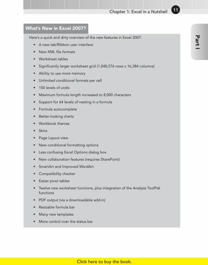
Here’s a quick and dirty overview of the new features in Excel 2007:

• A new tab/Ribbon user interface

• New XML file formats

• Worksheet tables

• Significantly larger worksheet grid (1,048,576 rows x 16,384 columns)

• Ability to use more memory

• Unlimited conditional formats per cell

• 100 levels of undo

• Maximum formula length increased to 8,000 characters

• Support for 64 levels of nesting in a formula

• Formula autocomplete

• Better-looking charts

• Workbook themes

• Skins

• Page Layout view

• New conditional formatting options

• Less confusing Excel Options dialog box

• New collaboration features (requires SharePoint)

• SmartArt and Improved WordArt

• Compatibility checker

• Easier pivot tables

• Twelve new worksheet functions, plus integration of the Analysis ToolPak functions

• PDF output (via a downloadable add-in)

• Resizable formula bar

• Many new templates

• More control over the status bar

What’s New in Excel 2007?

05_044025 ch01.qxp 1/2/07 10:57 PM Page 11



The Excel User InterfaceA user interface (UI) is the means by which an end user communicates with a computer pro-gram. A UI includes elements such as menus, dialog boxes, toolbars, and keystroke combi-nations, as well as features such as drag and drop.

A New User InterfaceAlmost every Windows program you use employs the menu and toolbar approach. That is,at the top of the screen is a menu bar that contains virtually every command that’s avail-able in the application and below that, one or more toolbars, which provide shortcuts tosome of the more frequently used commands. For Excel, and most of the other MicrosoftOffice applications, the days of menus and toolbars are over.

The new UI for Excel consists of components like the Ribbon, the Office Button, the MiniToolbar, and the Quick Access toolbar. The Quick Access toolbar is the only UI elementthat can be customized by end users.

The RibbonThe Ribbon is the primary UI component in Excel. It replaces the menu and most of thetoolbars that were common in previous versions, and is a very significant departure fromthe interfaces of most Windows-based applications.

ONE-STOP SHOPPINGMicrosoft felt that the commands contained in the old menu and toolbar system werebecoming so numerous that a new paradigm was necessary. One of the main goals fordeveloping the Ribbon was to provide the user with a single place to look for a particularfeature. Every commonly used command available in Excel would be contained in theRibbon (or in a dialog box accessed via the Ribbon). Although Microsoft succeeded inputting most of the available commands on the Ribbon, it’s still a pretty big place. Long-time Excel users will have to endure a certain amount of frustration while they get used tothe new layout.

NOTEA few commands failed to make the cut, but they are still available if you know where tolook for them. Right-click the Quick Access toolbar and choose Customize Quick AccessToolbar. Excel displays a dialog box with a list of commands that you can add to yourQuick Access toolbar (QAT). Some of these commands aren’t available elsewhere in the UI.

TABS, GROUPS, AND TOOLSThe Ribbon is a band of tools that stretches across the top of the Excel window. About thevertical size of three of the old style toolbars, the Ribbon sports a number of tabs includingHome, Insert, Page Layout, and others. On each tab are groups that contain related tools.


05_044025 ch01.qxp 1/2/07 10:57 PM Page 12



On the Home tab, for example, you find the Clipboard group, the Font group, and theAlignment group.

After you get past the Ribbon, the tabs, and the groups, you get to the tools, which aresimilar to the tools that existed on the old style toolbars with one major difference: theirdifferent sizes. Tools that are used most often are larger than less-frequently used tools.Half of the Clipboard group is consumed by the large Paste tool; the Cut, Copy, and FormatPainter tools are much smaller. Microsoft determined that the Paste tool is the most usedtool and thus sized it accordingly.

The Ribbon and all its components resize dynamically as the Excel window is resized hori-zontally. Smaller Excel windows collapse the tools on compressed tabs and groups, andmaximized Excel windows on large monitors show everything that’s available. Even in asmall window, all Ribbon commands remain available. You just may need to click a fewextra times to access them.

Figure 1-2 shows three sizes of the Ribbon when the Home tab is displayed using anincreasingly smaller horizontal window size.

Figure 1-2: The Ribbon sizes dynamically, depending on the horizontal size of Excel’s window.

NAVIGATIONNavigation of the Ribbon is fairly easy with the mouse. You click a tab and then click atool. If you prefer to use the keyboard, Microsoft has added a feature just for you. PressingAlt displays tiny squares with shortcut letters in them that hover over their respective tabor tool. Each shortcut letter that you press either executes its command or drills down toanother level of shortcut letters. Pressing Esc cancels the letters or moves up to the previ-ous level. For example, a keystroke sequence of Alt+H+B+B adds a double border to thebottom of the selection. The Alt key activates the shortcut letters, the H shortcut activatesthe Home tab, the B shortcut activates the Borders tool menu, and the second B shortcutexecutes the Bottom Double Border command. Note that it’s not necessary to keep the Altkey depressed while you press the other keys.


art I13

05_044025 ch01.qxp 1/2/07 10:57 PM Page 13



CONTEXTUAL TABSThe Ribbon contains tabs that are visible only when they are needed. Generally, when apreviously hidden tab appears, it’s because you selected an object or a range with specialcharacteristics (like a chart or a pivot table). A typical example is the Drawing Tools con-textual tab. When you select a shape or WordArt object, the Drawing Tools tab is made visible and active. It contains many tools that are only applicable to shapes, such as shape-formatting tools.

SCREENTIPS AND DIALOG ICONSHovering over a tool on the Ribbon displays a ScreenTip that explains the command thetool will execute. ScreenTips are larger and, in most cases, wordier than the ToolTips fromprevious versions. They range in helpfulness from one word to long paragraphs and evenpictures.

At the bottom of many of the groups is a small box icon (a dialog box launcher) that opens adialog box related to that group. Users of previous versions of Excel will recognize thesedialog boxes, many of which are unchanged. Some of the icons open the same dialog boxesbut to different areas. For instance, the Font group icon opens the Format Cells dialog boxwith the Font tab activated. The Alignment group opens the same dialog box but activatesthe Alignment tab. The Ribbon makes using dialog boxes a far less-frequent activity thanin the past because most of what can be done in a dialog box can be done directly on theRibbon.

GALLERIES AND LIVE PREVIEWA gallery is a large collection of tools that look like the choice they represent. If you’veused previous versions of Excel, you may have noticed that the font names in the drop-down box on the Formatting toolbar were in their own font. Galleries are an extension ofthat feature. The Styles gallery, for example, does not just list the name of the style butlists it in the same formatting that will be applied the cell.

Although galleries help to give you an idea of what your object will look like when anoption is selected, Live Preview takes it to the next level. Live Preview displays yourobject or data as it will look right on the worksheet when you hover over the gallery tool.By hovering over the various tools in the Format Table gallery, you can see exactly whatyour table will look like before you commit to a format.

The Office Button MenuAlthough menus are a thing of the past in Excel 2007, one holdout remains: the OfficeButton menu. In the upper-left corner of the Excel window is a round Microsoft Office logothat is known as the Office Button. Click it, and you see a traditional menu with menu com-mands (see Figure 1-3). Saving workbooks, opening workbooks, and printing are a few ofthe commands available.


05_044025 ch01.qxp 1/2/07 10:57 PM Page 14



Figure 1-3: Clicking the Office Button displays a menu, and some of the menu items havesubmenus.

The Office Button menu also contains the list of recent documents, just as it had in previ-ous versions. The recent documents list has undergone a major overhaul, however; themaximum number of documents on the list is now 50 from the previous of 9, with push-pinicons next to each entry that can be used to hold that document in its place on the listregardless of how many files you open and close.

At the bottom of the Office Button menu is the Excel Options button. This button opens theExcel Options dialog box, which contains dozens of settings for customizing Excel.

Shortcut Menus and the Mini ToolbarExcel also features dozens of shortcut menus. These menus appear when you right-clickafter selecting one or more objects. The shortcut menus are context sensitive. In other


art I15

05_044025 ch01.qxp 1/2/07 10:57 PM Page 15



words, the menu that appears depends on the location of the mouse pointer when youright-click. You can right-click just about anything — a cell, a row or column border, aworkbook title bar, and so on.

Right-clicking many items displays the shortcut menu as well as a Mini Toolbar. The MiniToolbar is floating toolbar that contains a dozen or so of the most popular formatting com-mands. Figure 1-4 shows the shortcut menu and Mini Toolbar when a range is selected.

Figure 1-4: The shortcut menu and Mini Toolbar appears when you right-click a range.

The Quick Access ToolbarThe Quick Access toolbar (or QAT) is a set of tools that the user can customize. By default,the QAT contains three tools: Save, Undo, and Redo. If you find that you use a particularRibbon command frequently, right-click the command and choose Add to Quick AccessToolbar. You can make other changes to the QAT from the Customization tab of the ExcelOptions dialog box. To access this dialog box, right-click the QAT and choose CustomizeQuick Access Toolbar.

Smart TagsA Smart Tag is a small icon that appears automatically in your worksheet after you com-plete certain actions. Clicking a Smart Tag reveals several clickable options.

For example, if you copy and paste a range of cells, Excel generates a Smart Tag thatappears below the pasted range (see Figure 1-5). Excel features several other Smart Tags,and additional Smart Tags can be provided by third-party providers.


05_044025 ch01.qxp 1/2/07 10:57 PM Page 16



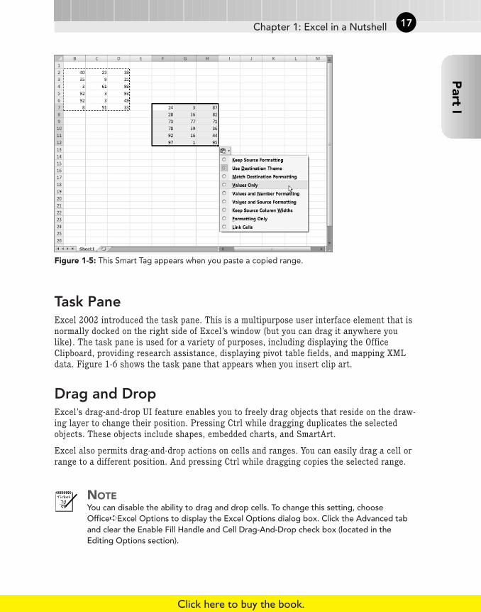
Figure 1-5: This Smart Tag appears when you paste a copied range.

Task PaneExcel 2002 introduced the task pane. This is a multipurpose user interface element that isnormally docked on the right side of Excel’s window (but you can drag it anywhere youlike). The task pane is used for a variety of purposes, including displaying the OfficeClipboard, providing research assistance, displaying pivot table fields, and mapping XMLdata. Figure 1-6 shows the task pane that appears when you insert clip art.

Drag and DropExcel’s drag-and-drop UI feature enables you to freely drag objects that reside on the draw-ing layer to change their position. Pressing Ctrl while dragging duplicates the selectedobjects. These objects include shapes, embedded charts, and SmartArt.

Excel also permits drag-and-drop actions on cells and ranges. You can easily drag a cell orrange to a different position. And pressing Ctrl while dragging copies the selected range.

NOTEYou can disable the ability to drag and drop cells. To change this setting, chooseOffice➪Excel Options to display the Excel Options dialog box. Click the Advanced taband clear the Enable Fill Handle and Cell Drag-And-Drop check box (located in theEditing Options section).


art I17

05_044025 ch01.qxp 1/2/07 10:57 PM Page 17



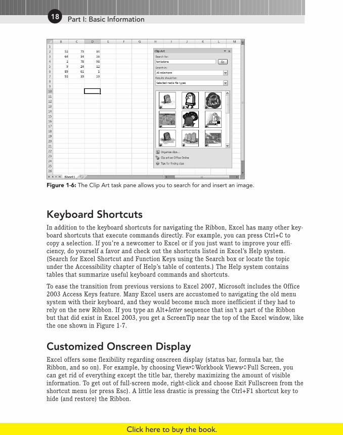
Figure 1-6: The Clip Art task pane allows you to search for and insert an image.

Keyboard ShortcutsIn addition to the keyboard shortcuts for navigating the Ribbon, Excel has many other key-board shortcuts that execute commands directly. For example, you can press Ctrl+C tocopy a selection. If you’re a newcomer to Excel or if you just want to improve your effi-ciency, do yourself a favor and check out the shortcuts listed in Excel’s Help system.(Search for Excel Shortcut and Function Keys using the Search box or locate the topicunder the Accessibility chapter of Help’s table of contents.) The Help system containstables that summarize useful keyboard commands and shortcuts.

To ease the transition from previous versions to Excel 2007, Microsoft includes the Office2003 Access Keys feature. Many Excel users are accustomed to navigating the old menusystem with their keyboard, and they would become much more inefficient if they had torely on the new Ribbon. If you type an Alt+letter sequence that isn’t a part of the Ribbonbut that did exist in Excel 2003, you get a ScreenTip near the top of the Excel window, likethe one shown in Figure 1-7.

Customized Onscreen DisplayExcel offers some flexibility regarding onscreen display (status bar, formula bar, theRibbon, and so on). For example, by choosing View➪Workbook Views➪Full Screen, youcan get rid of everything except the title bar, thereby maximizing the amount of visibleinformation. To get out of full-screen mode, right-click and choose Exit Fullscreen from theshortcut menu (or press Esc). A little less drastic is pressing the Ctrl+F1 shortcut key tohide (and restore) the Ribbon.


05_044025 ch01.qxp 1/2/07 10:57 PM Page 18



Figure 1-7: Using a keyboard sequence like Alt+I+R (for Insert➪Row) can still be used to insert arow and will display this ScreenTip during the process.

The status bar has also been enhanced in Excel 2007. Right-click the status bar, and yousee lots of options that allow you to control what information is displayed in the status bar.

Many other customizations can be made by choosing Office➪Excel Options and clicking theAdvanced tab. On this tab are several sections that deal with what displays onscreen.

Data EntryData entry in Excel is quite straightforward. Excel interprets each cell entry as one of thefollowing:

• A value (including a date or a time)

• Text

• A Boolean value (TRUE or FALSE)

• A formula

NOTEFormulas always begin with an equal sign (=).

Object and Cell SelectingGenerally, selecting objects in Excel conforms to standard Windows practices. You canselect a range of cells by using the keyboard (using the Shift key, along with the arrowkeys) or by clicking and dragging the mouse. To select a large range, click a cell at anycorner of the range, scroll to the opposite corner of the range, and press Shift while youclick the opposite corner cell.

You can use Ctrl+* (asterisk) to select an entire table. And when a large range is selected,you can use Ctrl+. (period) to move among the four corners of the range.


art I19

05_044025 ch01.qxp 1/2/07 10:57 PM Page 19



If you’re working in a table (created with the Insert➪Tables➪Table command), you’ll findthat Ctrl+A works in a new way. Press it once to select the table cells only. Press Ctrl+A asecond time, and it select the entire table (including the header and totals row). Press it athird time, and it selects all cells on the worksheet.


The following list of data-entry tips can help those moving up to Excel from anotherspreadsheet:

• To enter data without pressing the arrow keys, enable the After Pressing Enter,Move Selection option on the Advanced tab of the Excel Options dialog box(which you access from the Office➪Excel Options command). You can alsochoose the direction that you want to go.

• You may find it helpful to select a range of cells before entering data. If you doso, you can use the Tab key or Enter key to move only within the selected cells.

• To enter the same data in all cells within a range, select the range, enter theinformation into the active cell, and then press Ctrl+Enter.

• To copy the contents of the active cell to all other cells in a selected range, pressF2 and then Ctrl+Enter.

• To fill a range with increments of a single value, press Ctrl while you drag the fillhandle at the lower-right corner of the cell.

• To create a custom AutoFill list, select the Edit Custom Lists button on thePopular tab of the Excel Options dialog box.

• To copy a cell without incrementing, drag the fill handle at the lower-right corner of the selection; or, press Ctrl+D to copy down or Ctrl+R to copy to the right.

• To make text easier to read, you can enter line breaks in a cell. To enter a linebreak, press Alt+Enter. Line breaks cause a cell’s contents to wrap within the cell.

• To enter a fraction, enter 0, a space, and then the fraction (using a slash). Excelformats the cell using the Fraction number format.

• To automatically format a cell with the currency format, type your currency sym-bol before the value.

• To enter a value in percent format, type a percent sign after the value. You canalso include your local thousand separator symbol to separate thousands (forexample, 123,434).

• To insert the current date, press Ctrl+; (semicolon). To enter the current time intoa cell, press Ctrl+Shift+;.

• To set up a cell or range so that it accepts entries only of a certain type (or withina certain value range), use the Data➪Data Tools➪Data Validation command.

Data-Entry Tips

05_044025 ch01.qxp 1/2/07 10:57 PM Page 20



Clicking an object placed on the drawing layer selects the object. An exception occurs ifthe object has a macro assigned to it. In such a case, clicking the object executes themacro. To select multiple objects or noncontiguous cells, press Ctrl while you select theobjects or cells.

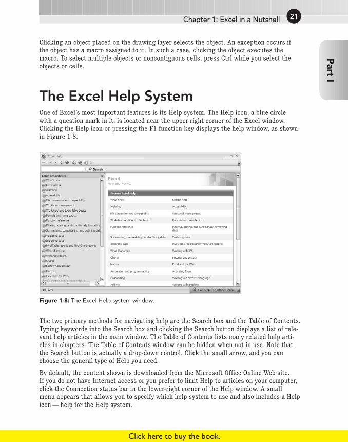
The Excel Help SystemOne of Excel’s most important features is its Help system. The Help icon, a blue circle with a question mark in it, is located near the upper-right corner of the Excel window.Clicking the Help icon or pressing the F1 function key displays the help window, as shownin Figure 1-8.

Figure 1-8: The Excel Help system window.

The two primary methods for navigating help are the Search box and the Table of Contents.Typing keywords into the Search box and clicking the Search button displays a list of rele-vant help articles in the main window. The Table of Contents lists many related help arti-cles in chapters. The Table of Contents window can be hidden when not in use. Note thatthe Search button is actually a drop-down control. Click the small arrow, and you canchoose the general type of Help you need.

By default, the content shown is downloaded from the Microsoft Office Online Web site. If you do not have Internet access or you prefer to limit Help to articles on your computer,click the Connection status bar in the lower-right corner of the Help window. A small menu appears that allows you to specify which help system to use and also includes a Helpicon — help for the Help system.


art I21

05_044025 ch01.qxp 1/2/07 10:57 PM Page 21



Cell FormattingExcel provides two types of cell formatting — numeric formatting and stylistic formatting.

Numeric FormattingNumeric formatting refers to how a value appears in the cell. In addition to choosing froman extensive list of predefined formats, you can create your own custom number formats inthe Number tab of the Format Cells dialog box . (Choose the dialog box launcher at the bot-tom of the Home➪Number group.)

Excel applies some numeric formatting automatically, based on the entry. For example, ifyou precede a value with your local currency symbol (such as a dollar sign), Excel appliesCurrency number formatting.

CROSS REFRefer to Appendix B for additional information about creating custom number formats.

The number format doesn’t affect the actual value stored in the cell. For example, supposethat a cell contains the value 3.14159. If you apply a format to display two decimal places,the number appears as 3.14. When you use the cell in a formula, however, the actual value(3.14159) — not the displayed value — is used.

Stylistic FormattingStylistic formatting refers to the cosmetic formatting (colors, shading, fonts, borders, andso on) that you apply in order to make your work look good. The Home➪Font and Home➪Styles groups contain all the commands that you need to format your cells and ranges.

A new formatting concept in Excel 2007 is document themes. Basically, themes allow you toset many formatting options at once, such as font, colors, and cell styles. The formattingoptions contained in a theme are designed to work well together. If you’re not feeling par-ticularly artistic, you can apply a theme and know the colors won’t clash. All the com-mands for themes are in the Themes group of the Page Layout tab.

Don’t overlook Excel’s conditional formatting feature. This handy tool enables you to spec-ify formatting that appears only when certain conditions are met. For example, you canmake the cell’s interior red if the cell contains a negative number. Excel 2007 includesmany new conditional formatting options, and the feature is much easier to use than in pre-vious versions.

CROSS REFSee Chapter 19 for more information on conditional formatting.


05_044025 ch01.qxp 1/2/07 10:57 PM Page 22



TablesA Table is a specially designated range in an Excel 2007 worksheet. If you used Lists inExcel 2003, you will already be familiar with some of what the Table object has to offer. Ifnot, don’t worry. Excel 2007 makes it easy to designate a range as a Table and makes iteven easier to perform many functions on that data.

The data in a table is related in a specific way. The rows represent related objects, and the columns represent specific pieces of information about each of those objects. If, forinstance, you have a table of library books, each row would hold the information for onebook. Columns might include title, author, publisher, date, and so on. In database terminol-ogy, the rows are records, and the columns are fields.

If your data is arranged in this fashion, you can designate it as a table by selecting therange and then choosing Insert➪Tables➪Table. Excel inserts generic column headings ifnone exist, color banding, and heading drop-down arrows into the data. These arrows, aswell as the Table Tools context tab on the Ribbon, provide quick access to many table-related functions like sorting, filtering, and formatting. In addition, using formulas withina table offers some clear advantages.

CROSS REFSee Chapter 9 for more information about the new Table feature in Excel 2007.

Worksheet Formulas and FunctionsFormulas, of course, make a spreadsheet a spreadsheet. Excel’s formula-building capabilityis as good as it gets. You will discover this as you explore subsequent chapters in thisbook.

Worksheet functions allow you to perform calculations or operations that would otherwisebe impossible. Excel provides a huge number of built-in functions, and Excel 2007 includesa few new functions. In addition, worksheet functions that formerly required the AnalysisToolPak add-in are now incorporated into Excel.

CROSS REFSee Chapter 4 for more information about worksheet functions.

Most spreadsheets allow you to define names for cells and ranges, but Excel handlesnames in some unique ways. A name represents an identifier that enables you to refer to a cell, range, value, or formula. Using names makes your formulas easier to create andread.


art I23

05_044025 ch01.qxp 1/2/07 10:57 PM Page 23



CROSS REFI devote Chapter 3 entirely to names.

Objects on the Drawing LayerAs I mention earlier in this chapter, each worksheet has an invisible drawing layer, whichholds shapes, SmartArt, charts, pictures, and controls (such as buttons and list boxes). Idiscuss some of these items in the following sections.

ShapesYou can insert a wide variety of shapes from Insert➪Shapes. After you place a shape onyour worksheet, you can modify the shape by selecting it and dragging its handles. In addi-tion, you can apply built-in shape styles, fill effects, or 3-D effects to the shape. Also, youcan group multiple shapes into a single drawing object, which you’ll find easier to size orposition.

IllustrationsPictures, clip art, and SmartArt can be inserted from the Insert➪Illustrations group.SmartArt replaces Diagrams from previous versions and have been expanded to includedozens of choices. Figure 1-9 shows some objects on the drawing layer of a worksheet.

Figure 1-9: Objects on a worksheet drawing layer. Excel makes a great doodle pad.


05_044025 ch01.qxp 1/2/07 10:57 PM Page 24



Linked Picture ObjectsA linked picture is a shape object that shows a range. When the range is changed, theshape object changes along with it. To use this object, copy a range and then chooseHome➪Clipboard➪Paste➪Paste As Picture➪Paste Picture Link. This command is useful if you want to print a noncontiguous selection of ranges. You can “take pictures” of theranges and then paste the pictures together in a single area, which you can then print.

ControlsYou can insert a number of different controls on a worksheet. These controls come in twoflavors — Form controls and ActiveX controls. Using controls on a worksheet and cangreatly enhance the worksheet’s usability — often, without using macros. To insert a con-trol, choose Developer➪Controls➪Insert. Figure 1-10 shows a worksheet with various controls added to the drawing layer.

NOTEThe Ribbon’s Developer tab is not visible by default. To show the Developer tab, chooseOffice➪Excel Options, navigate to the Popular tab, and check Show Developer Tab inthe Ribbon.

ON THE CDIf you’d like to see how these controls work, the workbook shown in Figure 1-10 is avail-able on the companion CD-ROM. The file is named worksheet controls.xlsx.

Figure 1-10: Excel enables you to add many controls directly to the drawing layer of a worksheet.


art I25

05_044025 ch01.qxp 1/2/07 10:57 PM Page 25



ChartsExcel, of course, has excellent charting capabilities. As I mention earlier in this chapter,you can store charts on a chart sheet or you can float them on a worksheet.

Excel offers extensive chart customization options. Selecting a chart displays the ChartTools contextual tab, which contain all the tools necessary to customize your chart. Right-clicking a chart element displays a shortcut menu.

You can easily create a free-floating chart by selecting the data to be charted and selectingone of the chart types from the Insert➪Charts group.

CROSS REFChapter 17 contains additional information about charts.

Customization in ExcelThis section describes two features that enable you to customize Excel — macros and add-ins.

MacrosExcel’s VBA programming language is a powerful tool that can make Excel perform other-wise impossible feats. You can classify the procedures that you create with VBA into twogeneral types:

• Macros that automate various aspects of Excel

• Macros that serve as custom functions that you can use in worksheet formulas

CROSS REFPart VI of this book describes how to use and create custom worksheet functions using VBA.

Add-in ProgramsAn add-in is a program attached to Excel that gives it additional functionality. For example,you can store custom worksheet functions in an add-in. To attach an add-in, use the Add-Ins tab in the Excel Options dialog box.


05_044025 ch01.qxp 1/2/07 10:57 PM Page 26



Excel ships with quite a few add-ins, and you can purchase or download many third-partyadd-ins from online services. My Power Utility Pak is an example of an add-in.

CROSS REFChapter 23 describes how to create your own add-ins that contain custom worksheetfunctions.

Internet FeaturesExcel includes a number of features that relate to the Internet. For example, you can savea worksheet or an entire workbook in HTML format, accessible in a Web browser. In addi-tion, you can insert clickable hyperlinks (including e-mail addresses) directly into cells.

CAUTIONIn Excel 2003, HTML was a round-trip file format. In other words, you could save a work-book in HTML format, reopen it in Excel, and nothing would be lost. That’s no longer thecase with Excel 2007. HTML is now considered an export-only format.

You can also create Web queries to bring in data stored in a corporate intranet or on theInternet.

Analysis ToolsExcel is certainly no slouch when it comes to analysis. After all, most people use a spread-sheet for analysis. Many analytical tasks can be handled with formulas, but Excel offersmany other options, which I discuss in the following sections.

Database AccessOver the years, most spreadsheets have enabled users to work with simple flat databasetables (even the original version of 1-2-3 contained this feature). Excel’s database featuresfall into two main categories:

• Worksheet databases: The entire database is stored in a worksheet. In Excel, a work-sheet database can have no more than 1,048,575 records (because the top row holds thefield names) and 16,384 fields (one per column).

• External databases: The data is stored outside Excel, such as in an Access MDB file orin SQL Server.


art I27

05_044025 ch01.qxp 1/2/07 10:57 PM Page 27



Generally, when the cell pointer resides within a worksheet database, Excel recognizes itand displays the field names whenever possible. For example, if you move the cell pointerwithin a worksheet database and choose the Data➪Sort & Filter➪Sort command, Excelallows you to select the sort keys by choosing field names from a drop-down list.

A particularly useful feature, filtering, enables you to display only the records that youwant to see. When Filter mode is on, you can filter the data by selecting values from pull-down lists (which appear in place of the field names when you choose the Data➪Sort &Filter➪Filter command). Rows that don’t meet the filter criteria are hidden. See Figure1-11 for an example.

If you convert a worksheet database into a table (by using Insert➪Tables➪Table), filteringis turned on automatically.

Figure 1-11: Excel’s Filter feature makes it easy to view only the database records that meet yourcriteria.

If you prefer, you can use the traditional spreadsheet database techniques that involve cri-teria ranges. To do so, choose the Data➪Sort & Filter➪Advanced command.

CROSS REFChapter 9 provides additional details regarding worksheet lists and databases.

Excel can automatically insert (or remove) subtotal formulas in a table that is set up as adatabase. It also creates an outline from the data so that you can view only the subtotalsor any level of detail that you desire.


05_044025 ch01.qxp 1/2/07 10:57 PM Page 28



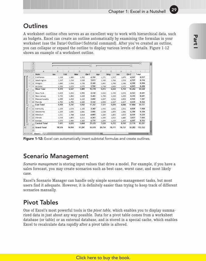
OutlinesA worksheet outline often serves as an excellent way to work with hierarchical data, suchas budgets. Excel can create an outline automatically by examining the formulas in yourworksheet (use the Data➪Outline➪Subtotal command). After you’ve created an outline,you can collapse or expand the outline to display various levels of details. Figure 1-12shows an example of a worksheet outline.

Figure 1-12: Excel can automatically insert subtotal formulas and create outlines.

Scenario ManagementScenario management is storing input values that drive a model. For example, if you have asales forecast, you may create scenarios such as best case, worst case, and most likelycase.

Excel’s Scenario Manager can handle only simple scenario-management tasks, but mostusers find it adequate. However, it is definitely easier than trying to keep track of differentscenarios manually.

Pivot TablesOne of Excel’s most powerful tools is the pivot table, which enables you to display summa-rized data in just about any way possible. Data for a pivot table comes from a worksheetdatabase (or table) or an external database, and is stored in a special cache, which enablesExcel to recalculate data rapidly after a pivot table is altered.


art I29

05_044025 ch01.qxp 1/2/07 10:57 PM Page 29



CROSS REFChapter 18 contains additional information about pivot tables.

As a companion to a pivot table, Excel also supports the pivot chart feature. Pivot chartsenable you to link a chart to a pivot table. In Excel 2007, pivot charts have improved significantly.

Auditing CapabilitiesExcel also offers useful auditing capabilities that help you identify errors or track the logicin an unfamiliar spreadsheet. To access this feature, choose commands in the Formulas➪Formula Auditing group.

CROSS REFRefer to Chapter 21 for more information about Excel’s auditing features.

Solver Add-inFor specialized linear and nonlinear problems, Excel’s Solver add-in calculates solutions to what-if scenarios based on adjustable cells, constraint cells, and, optionally, cells thatmust be maximized or minimized.

Protection OptionsExcel offers a number of different protection options. For example, you can protect formu-las from being overwritten or modified, protect a workbook’s structure, and protect yourVBA code.

Protecting Formulas from Being OverwrittenIn many cases, you may want to protect your formulas from being overwritten or modified.To do so, you must unlock the cells that you will allow to be overwritten and then protectthe sheet. First select the cells that may be overwritten and choose Home➪Cells➪Format➪Lock to unlock those cells. (The command toggles the Locked status.) Next,choose Home➪Cells➪Format➪Protect Sheet to show the Protect Sheet dialog. Here youcan specify a password if desired.

NOTEBy default, all cells are locked. Locking and unlocking cells has no effect, however, unlessyou have a protected worksheet.


05_044025 ch01.qxp 1/2/07 10:57 PM Page 30



Beginning with Excel 2002, Excel’s protection options have become much more flexible.When you protect a worksheet, the Protect Sheet dialog box (see Figure 1-13) lets youchoose which elements won’t be protected. For example, you can allow users to sort dataor use autofiltering on a protected sheet (tasks that weren’t possible with earlier versions).

Figure 1-13: Choose which elements to protect in the Protect Sheet dialog box.

You can also hide your formulas so they won’t appear in the Excel formula bar when thecell is activated. To do so, select the formula cells and press Ctrl+1 to display the FormatCells dialog box. Click the Protection tab and make sure that the Hidden check box isselected.

Protecting a Workbook’s StructureWhen you protect a workbook’s structure, you can’t add or delete sheets. Use the Review➪Changes➪Protect Workbook command to display the Protect Structure and Windows dialogbox, as shown in Figure 1-14. Make sure that you enable the Structure check box. If youalso mark the Windows check box, the window can’t be moved or resized.

Figure 1-14: The Protect Structure and Windows dialog box.


art I31

05_044025 ch01.qxp 1/2/07 10:57 PM Page 31



CAUTIONKeep in mind that Excel is not really a secure application. The protection features, evenwhen used with a password, are intended to prevent casual users from accessing variouscomponents of your workbook. Anyone who really wants to defeat your protection canprobably do so by using readily available password-cracking utilities.

Password-protecting a WorkbookIn addition to protecting individual sheets and the structure of the workbook, you canrequire a password to open the workbook. To set a password, choose Office➪Prepare➪Encrypt Document to display the Encrypt Document dialog box (see Figure 1-15). In thisdialog box, you can specify a password to open the workbook.

Figure 1-15: Use the Encrypt Document dialog box to specify a password for a workbook.


05_044025 ch01.qxp 1/2/07 10:57 PM Page 32



excel 2007 formulas sample book

Documents

excel skill

denythat excel

excel userinterface

brief history of excel

sample chapterchapter

outsold visicalc

time porting visicalc

history of excelyou