excel: functions and data analysis...

ACS Microcomputer Workshop

Excel: Functions and Data Analysis Tools Introduction The Excel software package consists of three basic parts: its electronic spreadsheet, graphics, and database utilities. Using a single set of data, these separate utilities can work together or individually. This workshop concentrates on defining Excel functions, using the function wizard, and using the Data Analysis Toolpak. Objectives The goal of this workshop is to introduce participants to the more complex features of Excel. After today's workshop participants will be able to:

• define terms used in creating functions • create and edit a function using the Function Wizard

• identify add-in functions • perform data analysis using Data Analysis Tools • create a formula with the Conditional Sum wizard • learn to trouble shooting a formula

Prerequisites: It is assumed that the participants in this workshop have either taken the Excel: Intermediate workshop or have equivalent skills. Other related workshops: Excel: Introduction Learn about Excel's menu selection, cursor movement, various data types, cell addressing, and Help as you build a simple worksheet. Edit data, set ranges, format information, and use AutoFormat to create finished tables. Prerequisite: Experience working in the Windows 95 or Mac OS environment. Requires registration for all and a $75 fee for non-University.

Excel: Functions and Data Analysis Tools 2 © 1999 University of Kansas

ACS Microcomputer Workshop

Excel: Functions & Data Analysis Tools Outline

DEFINITIONS The following definitions are necessary to understand the basics of creating Excel formulas and functions.

Formula A formula is an equation that analyzes data on your worksheet. Formulas perform calculations such as addition or multiplication; formulas can also combine values. In Excel, all formulas begin with an equal sign (=) and are followed by the data the formula calculates.

Formula syntax Formula syntax is the structure or order of the formula elements. All formulas begin with an equal sign (=) followed by operands (the data to be calculated) and the operators. Operands can be values that don't change (constants), a range reference, a label, a name, or a worksheet function.

Formula bar The formula bar is an area located at the top of the worksheet window that is used to enter or edit values or formulas in cells or charts. The formula bar displays the constant value or formula in the active cell. To display or hide the formula bar, click Formula Bar on the View menu.

Order of precedence Formulas are calculated left to right, using order of precedence, unless the use of parentheses changes the order of calculation.

Example: = 10 + 10*4 or = (10+10)*4

Excel performs operations in the order shown in the following table. If a formula contains operators with the same order of precedence, Excel evaluates the operators from left to right. For example, if you enter the formula, 7 + 7 – 5, the calculation is performed left to right since both + and – have the same precedence. If you enter the formula, 7 + 7 * 5, Excel performs the multiplication first since * has a higher precedence than +.

To change the order of evaluation, enclose the part of the formula to be calculated first in parentheses.

Operator Description

: (colon), (comma) (single space) Reference operators

– Negation (as in –1)

% Percent

^ Exponentiation


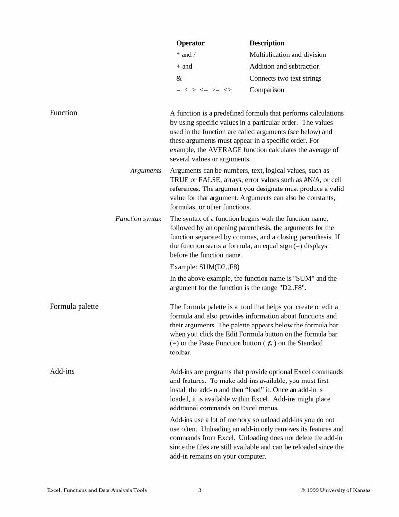
Operator Description

* and / Multiplication and division

+ and – Addition and subtraction

& Connects two text strings

= < > <= >= <> Comparison

Function A function is a predefined formula that performs calculations by using specific values in a particular order. The values used in the function are called arguments (see below) and these arguments must appear in a specific order. For example, the AVERAGE function calculates the average of several values or arguments.

Arguments Arguments can be numbers, text, logical values, such as TRUE or FALSE, arrays, error values such as #N/A, or cell references. The argument you designate must produce a valid value for that argument. Arguments can also be constants, formulas, or other functions.

Function syntax The syntax of a function begins with the function name, followed by an opening parenthesis, the arguments for the function separated by commas, and a closing parenthesis. If the function starts a formula, an equal sign (=) displays before the function name.

Example: SUM(D2..F8)

In the above example, the function name is "SUM" and the argument for the function is the range "D2..F8".

Formula palette The formula palette is a tool that helps you create or edit a formula and also provides information about functions and their arguments. The palette appears below the formula bar when you click the Edit Formula button on the formula bar (=) or the Paste Function button ( ) on the Standard toolbar.

Add-ins Add-ins are programs that provide optional Excel commands and features. To make add-ins available, you must first install the add-in and then “load” it. Once an add-in is loaded, it is available within Excel. Add-ins might place additional commands on Excel menus.

Add-ins use a lot of memory so unload add-ins you do not use often. Unloading an add-in only removes its features and commands from Excel. Unloading does not delete the add-in since the files are still available and can be reloaded since the add-in remains on your computer.


A list of all add-ins automatically installed when you install Excel are available in the Help menu. Select Help and click Contents and Index. Enter “add-in programs, installing” and select “Components installed with Microsoft Excel.”

You can also use Visual Basic programs as custom add-ins.

FUNCTION WIZARDS The Function Wizards are designed to help provide the

necessary arguments and descriptions for the various Excel functions.

General instructions for function wizards

To access the Function Wizard,

1. Select the cell in which you want the results of the function to display.

2. Click the Function Wizard button on the Standard toolbar ( )or select Function… from the Insert menu.

3. Select a function category from the list on the left of the Paste Function dialog box. A list of function names (grouped by category) displays on the right. To view all functions, click All on the Category list.

4. Double-click the function name listed on the right and the Function Palette displays.

The Function Palette displays input boxes and explan-

ations to provide the necessary function arguments. The palette also displays sample function results.


5. Enter the necessary arguments in the input boxes.

To select ranges on your worksheet, click beside the appropriate dialog box. Excel hides the Function Palette so that you can use your mouse to manually select the correct range(s). To return to the Function Palette, click

or press Return. 6. Click OK when you have finished entering arguments.

A sampling of functions using the Function Wizard

During the workshop, the following functions demonstrate the Function Wizard and Paste Function dialog box.

CONCATENATE The Concatenate function joins several text strings into one text string.

Syntax CONCATENATE (text1,text2,...)

Text1, text2, Text arguments are 1 to 30 text items that will be joined into a single item. The text items can be text strings, numbers, or single-cell references.

The "&" operator can be used instead of CONCATENATE to join text items.

CONCATENATE ("Academic ", "Computing ", "Services") is equivalent to "Academic Computing Services."

If cell A2 contains "Academic " and B2 contains "Computing " then CONCATENATE (A2,B2, "Services") is equivalent to "Academic Computing Services."

COUNT Counts the number of cells that contain numbers and numbers within the list of arguments.

Syntax COUNT(value1,value2, ...)

Value1, value2 Values are 1 to 30 arguments that can contain or refer to a variety of different types of data, but only numbers are counted.


COUNTA Counts the number of cells that are not empty and the values within the list of arguments. Use COUNTA to count the number of cells that contain data in a range or array.

Syntax COUNTA(value1,value2, ...)

Value1, value2 Values are 1 to 30 arguments representing the values you want to count. In this case, a value is any type of information, including empty text ("") but not including empty cells.

COUNTBLANK Counts empty cells in a specified range of cells. Cells with formulas that return "" (empty text) are also counted. Cells with zero values are not counted.

Syntax COUNTBLANK(range)

Range Range is the range of cells where you want to identify blank cells.

COUNTIF Counts the number of cells within a range that meet the given criteria

Syntax COUNTIF(range, criteria)

Range Range is the range of cells where you want to count cells.

Criteria Criteria are the form of a number, expression, or text that defines which cells will be counted. For example, criteria can be expressed as 123456, "123456", ">123456", "enrolled".

VLOOKUP In general lookup functions are used to lookup data in one list and return a corresponding value. Vlookup (vertical lookup) is one of several lookup functions but since data is generally organized in columns, vlookup is used frequently.

Syntax VLOOKUP(lookup_value, table_array, col_index_num, range_lookup)

Lookup_value The lookup_value is the value to be found in the first column of the table array. The lookup_value can be a value, a reference, or a text string.

Table_array Table_array is the table of information in which data is looked up. If you create a range name like List or Sales_Table, it is easy to copy the function without losing your reference to the table range. Otherwise you will need to use absolute addressing in specifying the table.

The values in the first column of table_array can be text, numbers, or logical values.


Col_index_num Col_index_num is the column number in the table_array from which the matching value must be returned. For example, a col_index_num of 2 returns the value in the second column in table_array.

If col_index_num is less than 1, VLOOKUP returns the #VALUE! error value; if col_index_num is greater than the number of columns in table_array, VLOOKUP returns the #REF! error value.

Range_lookup Range_lookup is a logical value that specifies whether you want VLOOKUP to find an exact match or an approximate match. If the range_lookup argument is omitted (TRUE), an approximate match is returned. If an exact match is not found, the next largest value that is less than lookup_value is returned. If FALSE, VLOOKUP will find an exact match and if an exact match is not found, the error value #N/A is returned.

Notes If range_lookup is TRUE, the values in the first column of table_array must be placed in ascending order, otherwise VLOOKUP may not give the correct value. If range_lookup is FALSE, table_array does not need to be sorted.

Example Lookup_value

Table A Rep Sales Bonus %

Fred 23000 =VLOOKUP

Mary 24000

Beth 16000

John 25000

Dave 32000

Janet 30000

Table_array

Table B Sales Level Bonus Rate

$0.00 0%

$10,000 4%

$20,000 6%

$30,000 8%

$40,000 12%

Using the above columns of data as an example, the VLOOKUP formula is placed in the Bonus Percent column of Table A.


The Sales column is the lookup value and, from Table B, the Sales Level column and the Bonus Rate columns comprise the table_array since you want to determine what rate should be paid for corresponding sales.

The col_index_num is 2 since the rate that you want to report is in the second column of the table_array.

The range_lookup is TRUE because we don't need to match the sales exactly. You can omit the range_lookup or type TRUE.

Note: Since the Sales value does not match the Sales Level exactly, Table B must be sorted in ascending values.

ADD IN COMMANDS AND FUNCTIONS

An Add-in is a command or function that, once loaded, appears to be a part of the Excel program. Add-in commands or functions may be user-created macros or may be the add-ins included with the Excel program. Some Excel add-ins are automatically loaded when Excel is installed; the user loads others. Not all add-ins are automatically loaded because add-ins use a lot of memory.

Loading an add-in Once an add-in is loaded, it is always available until you unload it.

1. On the Tools menu, click Add-Ins.

2. In the Add-Ins available box, click the check box next to the add-in you want to load. If the add-in you want to use is not listed in the Add-Ins available box, click Browse, and then locate the add-in. If the add-in is not installed on your computer, you must install it.

3. Click OK.

Unloading an add-in Unloading add-ins that you don’t use can save memory since all loaded add-ins are always loaded into memory when accessing Excel.

1. On the Tools menu, click Add-Ins.

2. In the Add-Ins available box, clear the check box next to the add-in you want to unload.

3. Click OK.

When you unload an add-in, the add-in macro is not deleted from your computer.


DATA ANALYSIS TOOLS The Analysis Tools are Excel Add-ins and take a few seconds to load when the command is first selected. The Analysis Tools command on the Options menu is available only if the Analysis ToolPak is installed. The Analysis Tools are one of several Add-ins available within Excel. Analysis Tools involve the collection, organization, and interpretation of numeric data.

Examples The analysis tool discussed here is the Histogram. The Data Analysis menu option (under the Tools menu) is not available until you have "loaded" it. See Loading an Add-in above.

Histogram example A histogram is an analysis tool that consolidates data into a range of numeric intervals to show how frequently the range contains similar values.

Setting up the data A histogram counts how many of the values in a range (input range) fall within specified numeric intervals (bin range).

For example, in a group of people, you could determine the distribution of ages within age categories.

You need to setup your worksheet before running the Histogram Data Analysis tool. You need to determine the following:

• The Input range or the range of values to analyze.

• The Bin range or the range of cells that contain a set of boundary values. (See below.) The Bin Range is optional.

• The Output range or an area to display the histogram.

Input Range In the example below, the ages column is the input range since this is the column of data to analyze.

Bin Range In the example below, the bin range contains the age intervals. When setting up a histogram, make sure the intervals for the bin range are specified in ascending order.

D


D 1 Bin 2 20 3 30 4 40 5 50 6 60

Output range The results of the distribution can be placed in an area on the current worksheet, on another worksheet within the same workbook, or in another workbook.

Creating the Histogram Before accessing the Histogram Analysis tool, make sure your worksheet is setup properly. See Setting up the data above. To create a histogram: 1. Choose Analysis Tool from the Tools menu 2. Select Histogram from the Data Analysis list box. 3. Click OK to display Histogram dialog box.

4. Enter the range of cells to analyze in the Input Range: input box.

5. Enter the Bin range in the Bin Range: input box. If you omit the bin range, Excel creates a set of evenly distributed bins between the data's minimum and maximum values.

6. Specify the output range. See Output options below:

Output Options Output Range: Enter the reference for the upper-left cell of the output table. The size of the output area is automatically determined and Excel displays a message if the output table might overwrite existing data.

New Worksheet Ply: Click to insert a new worksheet in the current workbook and paste the results starting at cell A1 of the new worksheet. You can name the worksheet by typing a name in the input area after selecting New Worksheet Ply.


New Workbook: Click to create a new workbook and paste the results on a new worksheet in the new workbook.

Other Histogram options 7. Select any other appropriate options. (See below for definitions.)

Labels: Select Labels if the first row or column of your input range contains labels. Clear this check box if your input range has no labels; Excel generates appropriate data labels for the output table.

Pareto: If the Pareto box is checked, the output data displays in descending frequency order in the output table.

Cumulative Percentages: If the Cumulative Percentages box is checked, Excel generates an output table column for cumulative percentages. Leave unchecked to omit the cumulative percentages.

Chart Output: Select Chart Output to generate an embedded histogram chart with the output table.

Conditional example Use the Conditional Sum Wizard to summarize values in a list based on specific conditions. The Conditional Sum Wizard can help you determine the number of people that meet a certain criteria. In the example below, the conditional sum function can determine how many people are on academic probation that transferred from other schools. In this example, there are two criteria that need to be defined and then a sum of those who meet both.

A B C 1 Name Status Change of School 2 Jim Enrolled Transfer 3 Mary Probation KU - College 4 Fred Enrolled KU - Business 5 Alice Enrolled Transfer

Start the wizard 1. Click a cell within the table or list.

2. On the Tools menu, point to Wizard, and then click Conditional Sum.

The Conditional Sum Wizard is an add-in program. If the Conditional Sum command is not on the Wizard submenu, install and load the wizard. (See Add-in commands and Functions above.)


3. Enter the information requested.

Use the pull-down menus to select available options for

the Column to Sum. Also use pull-down menus to determine the criteria of the data to sum.

Click the Add Condition button to add criteria to the list; you can define more than one criterion.

4. After all selections are complete, click Finish on the last dialog box.

ANAYLZING DATA WITH THE PIVOT TABLE

Definition

A PivotTable is an interactive table that summarizes, or cross-tabulates, large amounts of data. You can rotate rows and columns to view various summaries of data. You can also filter data by displaying different pages or display the details for areas of interest.

The PivotTable summarizes data by using a summary function that you specify, such as Sum, Count, or Average. You can include subtotals and grand totals automatically, or use your own formulas by adding calculated fields and items.

A Pivot Table wizard provides help in creating pivot tables.

Before creating a Pivot Table Before starting the Pivot Table wizard,

1. Your worksheet data must be organized in a list or database format. (See the Excel: Intermediate outline.)


2. Place your cursor inside the list.

3. Remove all subtotals created with Data, Subtotals command since grand and subtotals are automatically created as part of the pivot table. (See the Excel: Intermediate outline.)

General Pivot Table instructions Before beginning the Pivot Table Wizard, make sure you have followed the instructions above.

1. Select Pivot Table Report from the Data menu. The first step of the Wizard displays.

2. Identify the location of your Pivot Table data source. The default setting is an Excel list or database on your current worksheet. Click Next.

3. Select the range of cells that comprise your list. If your cursor is inside the list or database area, Excel selects the data automatically. You can redefine the list if necessary by using your mouse to select the data source and then press Enter to return to the dialog box.

4. Click Next.

5. A sample pivot table layout displays.

Any column labels on your list are displayed as buttons

and referred to as fields. Each field can be placed in one of four parts of the pivot table.

Row: Any field placed in the Row area becomes a row label.

Column: Any field placed in the column area becomes a column label.

Data: Any numeric field placed in the Data area is summarized (sum, average, etc.).

Page: Any field you want to use as a filter is placed the Page area.


Placing fields 6. To place a field in the pivot table, drag the field name to the appropriate area.

7. Click Next when the layout is complete.

8. Select the location for the pivot table. The default is to place the table on a new worksheet.

You can designate an area of an existing worksheet if you select Existing Worksheet and then use your mouse to identify the upper left corner of the Pivot Table.

You can also use your mouse to select another workbook; you can also designate a worksheet.

9. Click Finish.

Editing the Pivot Table You can edit and format many components of the Pivot Table. To select areas of the Pivot Table,

Table components Click Select Row Field All row labels Row item All item data Column field All column labels Column item All item data Summary label Entire table Grand Total label Column or row totals

Quick access to field dialog boxes Double-click the row or column fields to display the Pivot Field dialog box. If the above methods do not select, from the PivotTable tool bar (see below), click Select and Enable Selection.

Pivot table toolbar When a Pivot Table is displayed on a worksheet, the Pivot Table toolbar automatically displays.

Click to access the original Pivot Table wizard and to

access the Pivot Table Field dialog box. Both these buttons can be used to change the Pivot Table data display and values.

Deleting the Pivot Table To delete a Pivot Table,

1. On the PivotTable menu of the PivotTable toolbar, point to Select and select Enable Selection.


2. Click a cell in the PivotTable.

3. On the PivotTable toolbar, point to Select and then click Entire Table.

4. On the Edit menu, point to Clear, and then click All.

When you delete a PivotTable, the source data is not deleted or changed.

ARRAY FORMULAS An array formula is a formula that performs multiple

calculations and returns either a single result or multiple results. Array formulas act on two or more sets of values known as array arguments.

Each array argument must have the same number of rows and columns. You create array formulas the same way that you create basic, single-value formulas.

Entering an array formula To enter an array formula,

1. Select the cell or cells that contain the formula.

2. Enter the formula.

3. Press CTRL+SHIFT+ENTER to enter the formula within the cell. Brackets {} display around the entire formula, including the equal sign.

If you want only a single result, Excel may need to perform several calculations to generate that result.

TROUBLESHOOT ERRORS IN FORMULAS

If you have problems when creating functions, check the following to trouble-shoot your formulas.

Double-click on the cell that contains the formula to edit the formula. The worksheet ranges and the corresponding arguments within the formula display in colors to clearly define you formula arguments.

Parentheses are part of a matching pair. When you create a formula, Excel displays parentheses in color as they are entered.

Make sure you use the correct range operator when you refer to a range of cells. When you refer to a range of cells, use a colon (:) to separate the reference to the first cell in the range and the reference to the last cell in the range.


Make sure you have entered all arguments that are required and not any extras. Some functions have required arguments.

You can enter, or nest, no more than seven levels of functions within a function.

If the name of a workbook or a worksheet you refer to contains a non-alphabetic character, you must enclose the name within single quotation marks.

Make sure each external reference contains a workbook name and the path to the workbook.

Do not format numbers as you enter them in formulas. For example, even if the value you want to enter is $1,000, enter 1000 in the formula.

CONSULTING HELP Besides the Help options within the Excel program, Academic Computing Services provides consulting and Q&A help in a variety of ways: Phone Consulting 785/864-0410 Computer Help Center 785/864-0200 Online question account: [email protected] Online documentation: http://www.ukans.edu/acs/docs

To receive automatic announcements of upcoming computer training, send the following message to the e-mail address below: address: [email protected] message: SUB COMPUTER-TRAINING your name

Note: Substitute your name above for your real name, i.e. Jane Smith, not your login name.

Edited by: Jerree Catlin 785/864-0446

Academic Computing Services ©1999 The University of Kansas

Academic Computing Services April 2000


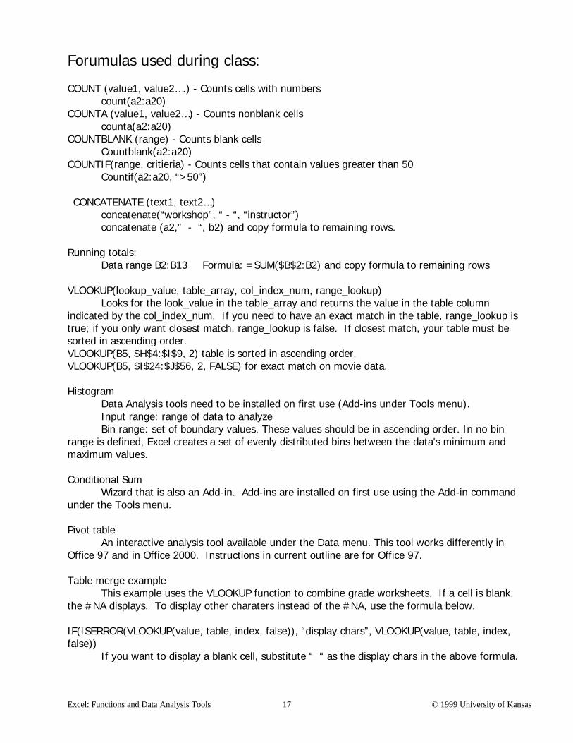
Forumulas used during class: COUNT (value1, value2….) - Counts cells with numbers count(a2:a20) COUNTA (value1, value2…) - Counts nonblank cells counta(a2:a20) COUNTBLANK (range) - Counts blank cells Countblank(a2:a20) COUNTIF(range, critieria) - Counts cells that contain values greater than 50 Countif(a2:a20, “>50”) –CONCATENATE (text1, text2…) concatenate(“workshop”, “ - “, “instructor”) concatenate (a2,” - “, b2) and copy formula to remaining rows. Running totals: Data range B2:B13 Formula: =SUM($B$2:B2) and copy formula to remaining rows VLOOKUP(lookup_value, table_array, col_index_num, range_lookup) Looks for the look_value in the table_array and returns the value in the table column indicated by the col_index_num. If you need to have an exact match in the table, range_lookup is true; if you only want closest match, range_lookup is false. If closest match, your table must be sorted in ascending order. VLOOKUP(B5, $H$4:$I$9, 2) table is sorted in ascending order. VLOOKUP(B5, $I$24:$J$56, 2, FALSE) for exact match on movie data. Histogram Data Analysis tools need to be installed on first use (Add-ins under Tools menu). Input range: range of data to analyze Bin range: set of boundary values. These values should be in ascending order. In no bin range is defined, Excel creates a set of evenly distributed bins between the data's minimum and maximum values. Conditional Sum Wizard that is also an Add-in. Add-ins are installed on first use using the Add-in command under the Tools menu. Pivot table An interactive analysis tool available under the Data menu. This tool works differently in Office 97 and in Office 2000. Instructions in current outline are for Office 97. Table merge example This example uses the VLOOKUP function to combine grade worksheets. If a cell is blank, the #NA displays. To display other charaters instead of the #NA, use the formula below. IF(ISERROR(VLOOKUP(value, table, index, false)), “display chars”, VLOOKUP(value, table, index, false)) If you want to display a blank cell, substitute “ “ as the display chars in the above formula.

excel: functions and data analysis...

Documents