Excel Smart

Guide80 Tips and Tricks on Excel

Become Smarter in Excel !

www.goodly.co.in

For more tips on Excel visit www.goodly.co.in | Goodly 2

Thanks for getting this EBookNow that you have this eBook, I am assuming that Excel holds a ton of value in your work life

and I am here just to give you that extra edge!

Every office has that one Excel Rock Star who is the apple of the boss’s eye when it comes to

analysis and number crunching in excel and needless to mention the perks that he enjoys!

“I want YOU to be that Rock Star”

How to use this book

I have written 80 tips & tricks under 9 different sections. These sections range from building

speed and productivity to working with data to charts and even VBA

Most articles are pretty comprehensive and have a link to my blog, where I have the detailed

explanation along with supplementary and additional resources that come along

Enjoy this eBook with a latte!

Share it !

• Does your friend or colleague use Excel ? Give it to him..

• Does your boss struggle with Excel ? Mail it to him

• Does your boyfriend / girlfriend work on Excel ? Send it to him/her (he/she will love you!)

• Does your ex use Excel at work ? Send it to him/her too (I do not know what will happen :D,

but it will help them too)

• The point is to share it with everyone you know who needs it!

You have my permission to print it and make as many copies as you like, provided you do not

change any content. But do not start selling it in any format. This eBook is free for you and for

everyone whom you share it with

You can find more tips and tricks on Excel on www.goodly.co.in

Yours Chandeep

For more tips on Excel visit www.goodly.co.in | Goodly 3

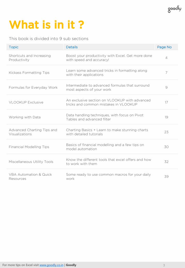
What is in it ?

Topic Details Page No

Shortcuts and Increasing

Productivity

Boost your productivity with Excel. Get more done

with speed and accuracy!4

Kickass Formatting TipsLearn some advanced tricks in formatting along

with their applications7

Formulas for Everyday WorkIntermediate to advanced formulas that surround

most aspects of your work9

VLOOKUP ExclusiveAn exclusive section on VLOOKUP with advanced

tricks and common mistakes in VLOOKUP17

Working with DataData handling techniques, with focus on Pivot

Tables and advanced filter19

Advanced Charting Tips and

Visualizations

Charting Basics + Learn to make stunning charts

with detailed tutorials23

Financial Modelling TipsBasics of financial modelling and a few tips on

model automation30

Miscellaneous Utility ToolsKnow the different tools that excel offers and how

to work with them32

VBA Automation & Quick

Resources

Some ready to use common macros for your daily

work39

This book is divided into 9 sub sections

For more tips on Excel visit www.goodly.co.in | Goodly 4

Section 1

Shortcuts for Increasing Productivity

Sno Shortcut What it does Quick Tip

1 CTRL + Arrow KeysJumps to the start and end of the data series

Use this a lot for navigating large workbooks, with many rows and columns. If you don’t know this already, you'll love me for this

2CTRL + PgUp / PgDn

Navigates to the next worksheet and to the previous worksheet

-

3 CTRL + SHIFT + L Applying and removing filter -

4 SHIFT + F11 Adding a new worksheet -

5 ALT > I > R Inserts a rowSelect multiple rows and then use the shortcut to insert multiple rows

6 ALT > I > C Inserts a columnSelect multiple columns and then use the shortcut to insert multiple columns

7 CTRL + D For copying downTo copy from first cell to the rest of the cells below it (contiguous range). The range needs to be selected first

8 CTRL + R For copying rightTo copy from first cell to the rest of the cells on the right (contiguous range). The range needs to be selected first

9 CTRL + 1Opens the format cell dialogue box

Also opens the format options for chart objects, shapes etc.. Click on any chart object (axis, labels, series) and press Ctrl + 1

10CTRL + SHIFT + -(minus sign)

Removes all borders from the selected cells

-

11 ALT > E > SOpens the Paste Special dialogue box

-

12 Function F4 Key

In the edit mode it allows you to change the cell reference from relative to absolute or semi-absolute

F4 Once – Locks row & column ($A$1), F4 Twice – Locks row (A$1), F4 Thrice – Locks column ($A1), F4 forth time - Remove cell locking (A1)

13ALT + = "equals sign"

Intelligently guesses the range/cells to Sum

-

14Ctrl + : (Colon Sign)

Enters the current date in the cell

15ALT > O > C > W Adjusting the width of the

columnThis is an old shortcut from Excel 2003 but still works a treat in all the versions till Excel 2013

Tip #1 : Top 15 Shortcuts that I recommend you to start with

For more tips on Excel visit www.goodly.co.in | Goodly 5

Section 1 : Shortcuts and Increasing Productivity

Tip #2 : 4 Awesome Lesser Known Shortcuts

Tip #3 : Download 100+ Excel Shortcuts pdf

1

2

Enter Data in multiple cells at once

1. Select Multiple Cells where you want to enter data

2. Start typing your data. For E.g. “Chandeep”

3. When done typing, press Ctrl Enter (instead of just pressing enter)

4. Chandeep will be added to all the cells selected

Use the shortcut ALT + ; to select only Visible Cells

Quick Tip : Use it to select only filtered cells while applying filter

3 Use the shortcut CTRL Shift O (the letter ‘o’) select all cells with comments

4 Use CTRL+' to copy a formula from above cell and open it in the edit mode

If you would like to be a shortcut frenzy, here is my list of 100 + Excel Keyboard Shortcuts (Downloadable

PDF). Enjoy!

Tip #4 : Watch Window in Excel

Watch windows are an amazing way to keep track of critical cells in your model or MIS. Here is a quick

example

We have the total and average of 150 records on Sheet 2. The

back up data is on Sheet 1

Now each time the back up data changes (on Sheet 1) you either

have to memorize the total or come back to Sheet 2 to see the

revised value

Learn to create Watch Windows to track cells live

For more tips on Excel visit www.goodly.co.in | Goodly 6

Section 1 : Shortcuts and Increasing Productivity

Tip #5 : 10 Excel Habits that you must Develop

Tip #6 : Border Shortcuts

I must recommend you these 10 habits that have saved me countless hours of manual work, made me

extremely productive and attained more refined and accurate output. Here you go!

10 Excel Habits, You Must Develop

If you are one of those who is into applying borders to almost

everything that you do in Excel, then you are going to fall in love

with these shortcuts and me of course!

Here are a few Exclusive Border Shortcuts in Excel

For more tips on Excel visit www.goodly.co.in | Goodly 7

This picture speaks miles about what we are going to discuss.

Get your eyes off the picture and lets get started .. shall we? I think the best way to start is to tell you that

custom formatting does not actually change the underlying data, but only changes the way it looks!

What if you boss asks you to format the following data

1. All the positive sales/profit numbers should appear this way $ 173.0 Mn

2. All negative (profit) numbers should appear this way in red color $ (14.0) Mn

3. All zeros should be replaced with a hyphen –

How would you do it ?

Learn Custom Formatting in Detail

Section 2

Kickass Formatting Tips

Tip #7 : Custom Formatting

For more tips on Excel visit www.goodly.co.in | Goodly 8

Section 2 : Kickass Formatting Tips

Tip #8 : 4 Custom number formats

You’ll have a better grip on this tip, if you have followed through the previous post. I have given some

more details about date formatting here 4 Quick Custom Formats for Dates

Tip #9 : Beauty Tips for your Excel Reports

If you tired of making obsolete looking Dashboards/Reports then I have 6 awesome (and equally simple)

make over tips for you.

We won’t go overboard in decking up our report until it looks horrible and meaning less but just enough

to make it classy and beautiful!

Read all the tips here - 6 Beauty Tips for your Excel Reports

For more tips on Excel visit www.goodly.co.in | Goodly 9

Section 3

Formulas for Everyday Work

Tip #10 : Where to use to IF, Nested IF and AND Functions

Here is a simple way to find out which one is the most appropriate logical statement under different

scenarios

• Use IF : When you have a single condition to test

• Use Nested IF (if inside another if) : When you have 2 conditions to test but one condition is

subsequent to other

For eg =IF(Sales < 80% of Target , IF(Attendance>75%, 10% Bonus, No Bonus), 15% Bonus)

In the above example, If the person has achieved less than 80% of target sales only then it checks

for attendance i.e. attendance condition is subsequent to sales target condition

• Use AND : When you have 2 conditions to test at the same time

For eg =IF( AND(Sales < 80% of Target , Attendance>75%), 15% Bonus, No Bonus)

In the above example the person has to meet sales and attendance targets to get the bonus. Then

I surround the AND statement in the IF statement to give out bonus or no bonus

=IF

=IF(CONDITION, IF(

=AND

What should

I use?

Tip #11 : Replace IF with MIN / MAX Functions

Take a look at a creative way to solve the IF problem without using IF. In this case we pay a 10% interest

only if there is Debt on the company

Long approach using IF Smart approach using MAX Statement

For more tips on Excel visit www.goodly.co.in | Goodly 10

Section 3 : Formulas for Everyday Work

Tip #12 : Cell Referencing Tricks

As you delve deeper into excel formulas you have to be insanely good at Cell referencing. Cell referencing

helps you write robust excel formulas and help you save you a ton of time. Read about cell referencing in

detail here – Cell Referencing in Excel (A must read)

Tip #13 : Interesting Facts about Dates

The excel calendar begins on 1st Jan 1900. Excel has represented every date with a number so 1st Jan

1900 is stored as the number 1 in Excel’s memory, 2nd Jan 1900 is stored as the number 2 and so on...

Excel has stretched the calendar till 31st-Dec-9999, numbered as 2958465 (I am not sure if we are going

to go that far in any sort of calculations, at-least I have not)

Quick Check

1. Type 1 in any cell

2. Covert that into a date format by pressing CTRL SHIFT 3

3. Now check the date (in the formula bar)

4. Isn’t that 1 Jan 1900?

1 Jan 1900Starting Date in Excel

31 Dec 9999Last date in Excel

Numbered as 1,2,3,4,5…………………………………………………………………………………………………..2958465 Last Date Number

Dates are +ve numbers in Excel

Tip #14 : Enter Today’s Date with a Shortcut

Use the shortcut CTRL ; (colon) to enter today’s date. The date input is a fixed value and won’t change to

the next date if you re open the same workbook the next day

Tip #15 : Enter Today’s Date with a Formula

Use the formula =TODAY() to enter today’s date. The date input is a dynamic and will change to the next

date if you re open the same workbook the next day

For more tips on Excel visit www.goodly.co.in | Goodly 11

Section 3 : Formulas for Everyday Work

Tip #16 : Time Stamp Problem and Circular Referencing in Formulas

Lets say we need a time stamp against every data entered but the condition is that once the time is

stamped against the data it cannot be changed.

We would use a simple IF formula for this but with a new concept called Circular Referencing

Introducing Circular Referencing – One or more cell references in a circular formula circles back to itself.

For example.. IF you type the following in Cell A10

=IF(A10<1000, A10+1, A10)

Each time we run the formula (pressing F9) the value in A10 will goes up by 1.

Setting Iterations for Circular Formulas – Although the formula is made in such a way that it will increase

the value by 1 each time but the number of iterations that are set in excel settings for circular formulas

can change the result.

Turning ON Iterative calculations - Excel Options (Alt > F > T) > Formulas > Check Iterative Calculations

It is a Circular Formula

Check this Option

Circular loop stops after 100 iterations

Now that we have understood circular referencing, let’s make a circular referencing formula. Be sure to

turn ON circular referencing

The IF Formula is checking IF1. Cell B9 is empty if it is Empty then it

gives nothing2. If not empty then it checks IF cell c9 is

empty (here the circular referencing starts)

3. If cell c9 is empty then it enters the current time and date using NOW function else gives the value of C9

For more tips on Excel visit www.goodly.co.in | Goodly 12

Section 3 : Formulas for Everyday Work

Tip #17 : DATEDIF Function to calculate between 2 dates

Somethings just stay evergreen, just like the DATEDIF function! Back in day

(days of Excel 2003) it used to be a stud amongst the Date Functions and it has

not lost its sheen till date but the newer versions of excel (2007 and above)

have stopped giving any help or guidance with this function

What it does: It returns the difference between two date values in either days,

months, years or some other mixed formats. Since there is no screen guidance

available when you type =DATEDIF you’d have to learn the syntax.

Learn the DATEDIF Function here

Tip #18 : WORKDAY.INTL & NETWORKDAYS.INTL functions to factor in holidays &

weekends

Syntax: WORKDAY.INTL(start_date, days, [weekend], [holidays])

How does it work: This function is very powerful for professionals in project management. This function

will return the next working day from a specific start date, taking care of weekends and holidays in

between. Lets understand the syntax

1. Start_date – This is the start date from where you want to start counting the number of working days

2. Days - This is the number of days you want ahead of the start date

3. Weekends – Excel gives you a help in order to choose your weekend pattern. For example if you

specified 1 i.e.. Saturday & Sunday or if you specified 2 i.e.. Sunday & Monday and so on. You can omit

this input, excel automatically considers Saturday & Sunday as default options

4. Holidays – These are the list of holidays (apart from Weekends) that you may want to specify. Excel will

automatically adjust in case of any overlap between holidays and weekends.

In the above example, we first linked the project start date as our Start_date and we linked the number of

days as 250. As soon as we move to the 3rd input excel drops down an automatic help for selecting the

weekend. Here we have chosen 1 for selecting Saturday and Sunday as weekends

As a last part of the input choose the range where you have specified the list of holidays. Here the result is

11 April 2014 that means that after considering 250 working days (excluding Saturday, Sundays and

Holidays) the project will end on 11 April 2014

For more tips on Excel visit www.goodly.co.in | Goodly 13

Section 3 : Formulas for Everyday Work

Tip #19 : WORKDAY.INTL & NETWORKDAYS.INTL functions to factor in holidays &

Weekends Continued..

Syntax: NETWORKDAYS.INTL(start_date, end_date, [weekend], [holidays])

How does it work: This function is the exact opposite of the WORKDAY.INTL function it calculates the

number of days between 2 dates taking care of weekends and holidays. Since the syntax is pretty similar

to the WORKDAY.INTL function lets look at a comprehensive example to understand this better

In the last input choose the range where you have specified the list of holidays. Here the result is 205 that

means that next appraisal date will come after 205 working days (excluding Sundays and Holidays)

Just like the earlier example, we first linked the appraisal start date as our Start_date and linked the next

appraisal date as our end_date. As soon as we move to the 3rd input, excel drops down an automatic help

for selecting the weekend. Here we have chosen 11 for selecting only Sunday as weekends

Tip #20 : Generating Serial Numbers with a Formula

Here is a Quick Tip to generate serial numbers

For more tips on Excel visit www.goodly.co.in | Goodly 14

Tip #21 : Trim Spaces and Ghost Spaces between your text

If you have been using the Trim function for a while to delete the

extra spaces between your text, you may have encountered that

sometimes the TRIM just doesn’t work!

Take a complete heads down on the TRIM Function and what to do

when TRIM function does not work

TRIM Function Workings and When TRIM function Fails to detect

ghost spaces

Tip #22 : Formula Auditing Techniques

To Err is to Human and to correct that err

is to audit your formulas. In this article I

talk about how can we effectively audit

our formulas in different ways.

I have 5 smart tricks here which you can

use for various needs!

1. Auditing with F2 Key - This is the most basic type of auditing but works a treat.

All you need to do is to press the F2 key to see which cells are linked to your

formulas (linking is shown by color coding). The formula bar also shows your

formulas but one can’t really make a head and tail out of it (since it shows no

linking)

Section 3 : Formulas for Everyday Work

Read the rest 4 Formula Auditing techniques

For more tips on Excel visit www.goodly.co.in | Goodly 15

Section 3 : Formulas for Everyday Work

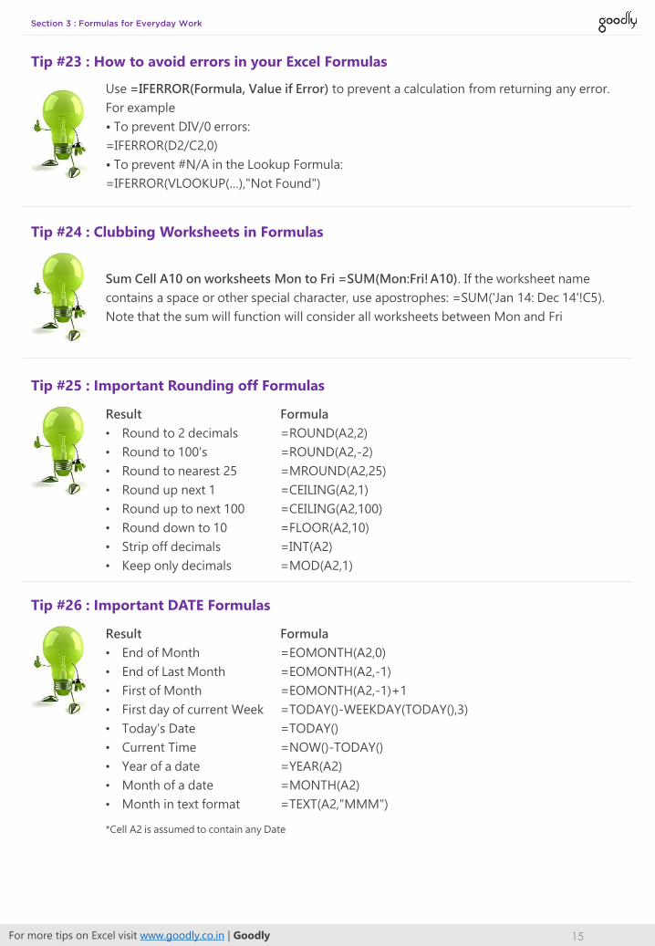
Tip #23 : How to avoid errors in your Excel Formulas

Use =IFERROR(Formula, Value if Error) to prevent a calculation from returning any error.

For example

• To prevent DIV/0 errors:

=IFERROR(D2/C2,0)

• To prevent #N/A in the Lookup Formula:

=IFERROR(VLOOKUP(…),"Not Found")

Tip #24 : Clubbing Worksheets in Formulas

Sum Cell A10 on worksheets Mon to Fri =SUM(Mon:Fri!A10). If the worksheet name

contains a space or other special character, use apostrophes: =SUM('Jan 14: Dec 14'!C5).

Note that the sum will function will consider all worksheets between Mon and Fri

Tip #25 : Important Rounding off Formulas

Result Formula

• Round to 2 decimals =ROUND(A2,2)

• Round to 100's =ROUND(A2,-2)

• Round to nearest 25 =MROUND(A2,25)

• Round up next 1 =CEILING(A2,1)

• Round up to next 100 =CEILING(A2,100)

• Round down to 10 =FLOOR(A2,10)

• Strip off decimals =INT(A2)

• Keep only decimals =MOD(A2,1)

Tip #26 : Important DATE Formulas

Result Formula

• End of Month =EOMONTH(A2,0)

• End of Last Month =EOMONTH(A2,-1)

• First of Month =EOMONTH(A2,-1)+1

• First day of current Week =TODAY()-WEEKDAY(TODAY(),3)

• Today's Date =TODAY()

• Current Time =NOW()-TODAY()

• Year of a date =YEAR(A2)

• Month of a date =MONTH(A2)

• Month in text format =TEXT(A2,"MMM")

*Cell A2 is assumed to contain any Date

For more tips on Excel visit www.goodly.co.in | Goodly 16

Section 3 : Formulas for Everyday Work

Tip #27 : Some Other Useful Functions

Result Formula

• Metric conversions =CONVERT(A2,"km","mi")

• Largest Value =MAX(A2:A99)

• 2nd Largest Value =LARGE(A2:A99,2)

• Smallest Value =MIN(A2:A99)

• 3rd Smallest Value =SMALL(A2:A99,3)

• Random number between 10 & 50 = RANDBETWEEN(10,50)

Tip #28 : How to find Calendar and Indian Quarter of a Date

How would you find out quarters for a given set of dates. For example

• 02-Feb-2014 is the 1st Quarter

• 15-Apr-2013 is the 2nd Quarter

• 27-Aug-2010 is the 3rd Quarter

There are 2 ways to solve this

1. Through VLOOKUP

2. Using some Math Formulas

The problem gets even more interesting when you are asked to find out Indian quarters for the dates as

per Indian Financial Year (Apr – Mar). For example

• 02-Feb-2014 is the 4th Quarter

• 15-Apr-2013 is the 1st Quarter

• 27-Aug-2010 is the 2nd Quarter

Read the full post – How to find quarters for Dates

For more tips on Excel visit www.goodly.co.in | Goodly 17

Section 4

VLOOKUP Exclusive !

Tip #29 : Comprehensive Guide to VLOOKUP and Tricks

We look up! Ha Ha!

Right from basics to being a pro at applying VLOOKUP, I have put down a short guide to help you learn

VLOOKUP. No jargons, just plain English!

I have also put together a short video guide for some awesome tricks that you can apply to your

VLOOKUP formulas

Comprehensive VLOOKUP Guide and Crazy Tricks (Video)

VLOOKUP facts & myths that I have witnessed.. pretty

interesting!

• “Do you know how to apply a VLOOKUP” ? It is one of the

most asked questions in the technical round of excel

interview. FACT

• If one knows how to apply VLOOKUP, he knows advanced

Excel or he is the master of Excel – MYTH

• VLOOKUP is difficult to learn – BIG MYTH

• The TRUE/FALSE input at the end of VLOOKUP is the same and

gives you the same result – MYTH

Tip #30 : Do you suffer from VLOOKUPHOBIA (the fear of applying a VLOOKUP) ?

If you pray to God for making your VLOOKUP work

“Oh God .. please make this VLOOKUP work !! I promise to visit you every

week “

Then you must read this – Suffering from VLOOKUPHOBIA?

In this post I will rescue you from the top 3 common mistakes while writing

VLOOKUP function and save your prayers for more crucial things in life!!

For more tips on Excel visit www.goodly.co.in | Goodly 18

Section 4 : VLOOKUP Exclusive !

Tip #31 : How to VLOOKUP similar (but not matching) records ?

It is often found in data sets that there are similar records but are not an exact match. How do you

perform a VLOOKUP on them?

Learn How to Apply Fuzzy Lookup in Excel

Tip #32 : How to perform a Picture VLOOKUP ?

Looking up pictures can be interesting and can possibly be used in different scenarios. Here is a quick

sneak peak into how can you do a Picture VLOOKUP

For more tips on Excel visit www.goodly.co.in | Goodly 19

Section 5

Working With Data

Tip #33 : Make your Filter work faster with Advanced Filter

Contrary to the name “Advanced filter”, I think Advanced Filter is more easy to use and offers a great

utility than the usual filter in Excel. Make your life simple by using Advanced Filter in Excel

Tip #34 : Make your life even simpler by Automating Advanced Filter using a Macro

Here is a quick guide (a short macro code) to automate your advanced filter. Automate Advanced Filter

For more tips on Excel visit www.goodly.co.in | Goodly 20

Section 5 : Working With Data

Tip #35 : How to Filter Pictures in your Data ?

Have you thought or faced a problem while filtering pictures in your data set? The solution is insanely

simple How to Filter Pictures

Tip #37 : How to inverse your Data

Have you ever had a situation where you wanted to inverse the order of your data? .. If yes then this is just

for YOU! You can do it with a simple Excel Formula How to Inverse your data?

Tip #36 : How to NOT Copy hidden rows from Filtered Data

Often the hidden rows also get copied when you copy the filtered data and paste it to the desired

location. To fix this problem all it takes is one additional step and 5 sorry 2 seconds extra than the normal

copy paste of the filtered data. Learn How NOT to copy hidden rows from Filtered Data

For more tips on Excel visit www.goodly.co.in | Goodly 21

Section 5 : Working With Data

Tip #38 : Add Multiple Data sets to your Pivot Table with Data Model

A data model (Excel 2013 feature) can link multiple data sets (converted

into tables) and make a single pivot table.

It additionally has a few new formulas for advanced analysis.. let’s not

just talk about it but experience it!! Ready for the steroid ?

Read Data Models in Excel 2013

(If you want to become an advanced Pivot Table user, It is a must read !)

With Data Model you can put your

Pivot Table on steroids!

Tip #39 : Do customized calculations by adding Calculated Fields in Pivot Tables

One of the less known and extremely awesome feature of Pivot Tables is its

ability to create calculated fields with in the Pivot Table. This makes your

Pivot Table calculations more versatile

Take a look at a Case Study on How to Add Calculated Fields in Pivot Tables

Tip #40 : Convert Dates in Quarters, Months or Years by Grouping feature in Pivot

The Grouping feature is a pretty awesome (and incredibly quick) technique to

do time series (quarters, years, months or more types of) analysis with a

couple of clicks. Also (over the years) I have realized that a lot of people don’t

know about this. Nothing better than if you know it

Take a dive into – Grouping Feature in Pivot Tables

For more tips on Excel visit www.goodly.co.in | Goodly 22

Section 5 : Working With Data

Tip #41 : How to Turn off the GETPIVOTDATA Function

GETPIVOTDATA can be quite irritating at times when you are trying to link a cell in the

Pivot Table Here is a quick way to turn it off. Turn off GETPIVOTDATA

For more tips on Excel visit www.goodly.co.in | Goodly 23

Section 6

Advanced Charting Tips & Visualizations

Tip #42 : Draw a Chart in 1 keystroke

Tip #43 : Learn the Basics of Charting in Excel

How to Draw the chart in 1 key stroke ?

1. Chart Types and How to create a Chart ? – Charting Basics Part 1

2. Adding / Editing data to your charts & How to work with different chart elements – Charting Basics

Part 2

3. Chart Formatting Essentials – Charting Basics Part 3

Tip #44 : A Quick Chart formatting Tip

Learn how to quickly replicate formatting to Raw Chart. Quick Chart Formatting Tip

For more tips on Excel visit www.goodly.co.in | Goodly 24

Section 6 : Advanced Charting Tips & Visualizations

Tip #45 : How to Pick the right color for your Chart

If you struggle to get the right mix of colors for your charts and visualizations? This one is for you.

Unfortunately Microsoft’s standard color selection is too lame to get it right the first time.

I am including in here as much as I know about colors and the techniques that have worked pretty well for

me to make my charts communicate effectively. Here you go - How to pick up right color for your Charts

Tip #46 : How to add Direct Legends to the Charts

When you are dealing with multiple series of data, especially in a line chart, it may become difficult to

match the line color with the legend. The quick solution is to add the legend at the end of the line chart.

Here is how you do it – How to add Direct Legends to the Charts

Tip #47 : How to make a Dynamic Stock Ticker Chart

You would have seen this Chart numerous times if look at stock prices. Can we draw it in Excel? Of course

we can – Presenting the Stock Ticker Chart for you!

For more tips on Excel visit www.goodly.co.in | Goodly 25

Section 6 : Advanced Charting Tips & Visualizations

A check button chart is extremely helpful when you want to give the user the choice of what she wants to

display in the chart and it looks equally sexy. All it takes is a bit of logic and a simple set of procedures to

follow. Learn to Make a Check Button Chart (A must learn chart technique to make your boss happy!)

Tip #48 : How to make a Check Button Chart

Tip #49 : Sparkline Charts

These are cute little compatible charts that fit in one cell. Like the default charts they don’t offer deep

analysis but are amazing for quick glances and basic insights and the best part is that they are damn easy

to create – Sparklines in Excel

For more tips on Excel visit www.goodly.co.in | Goodly 26

Section 6 : Advanced Charting Tips & Visualizations

Waterfall Chart (because it looks like a waterfall) is an awesome way to display how things add up to form

the total - How to Make a Waterfall Chart

Tip #50 : Learn to make the Waterfall Chart

Tip #51 : How to highlight Max and Min Points in your Chart

Use this technique in a line chart to dynamically highlight minimum and maximum data points. How to

Highlight Max and Min Points in your Chart

For more tips on Excel visit www.goodly.co.in | Goodly 27

Section 6 : Advanced Charting Tips & Visualizations

Here is a chart in which you can pick up which value you want to highlight (dotted border around it). It is

pretty simple to build it but looks stunning in your reports and dashboards. Highlight any data series in

your chart

Tip #52 : Customize highlighting any data series to focus on specific elements

Pick up any name in the drop down to highlightIt on the chart

Tip #53 : How to plot cities on a Map

As you pick up the city, it gets plotted on the Map

If you have always wondered a chart type where you can plot the city on a map and moreover if that can

be possible in Excel? It is right here!

In this post

• I have outlined the detailed working of this chart

• A video

• And downloadable files for your convenience

How to plot cities on Map using Excel

For more tips on Excel visit www.goodly.co.in | Goodly 28

Section 6 : Advanced Charting Tips & Visualizations

Tip #54 : Make Charts with REPT function (quick & easy)

It is so much fun using Excel in diversified ways. You can cleverly use the REPT function to make stunning

charts in Excel.. sounds bizarre and interesting? Lets explore this REPT Function Chart in Excel

Tip #55 : Scrolling List in Excel

Typically while summarizing your data if you run out of space to display all the information in a single

snap shot, here is a powerful method to create a scrolling list from your data set. All it takes is a few

minutes to set it up but creates a lasting impression in front of your boss/client.

Learn How to create a scrolling list in Excel

Tip #56 : How to add total to stacked column chart

Here is a quick trick to add total label to the stack bar chart. – Check it out Adding total to Stacked Chart

For more tips on Excel visit www.goodly.co.in | Goodly 29

Section 6 : Advanced Charting Tips & Visualizations

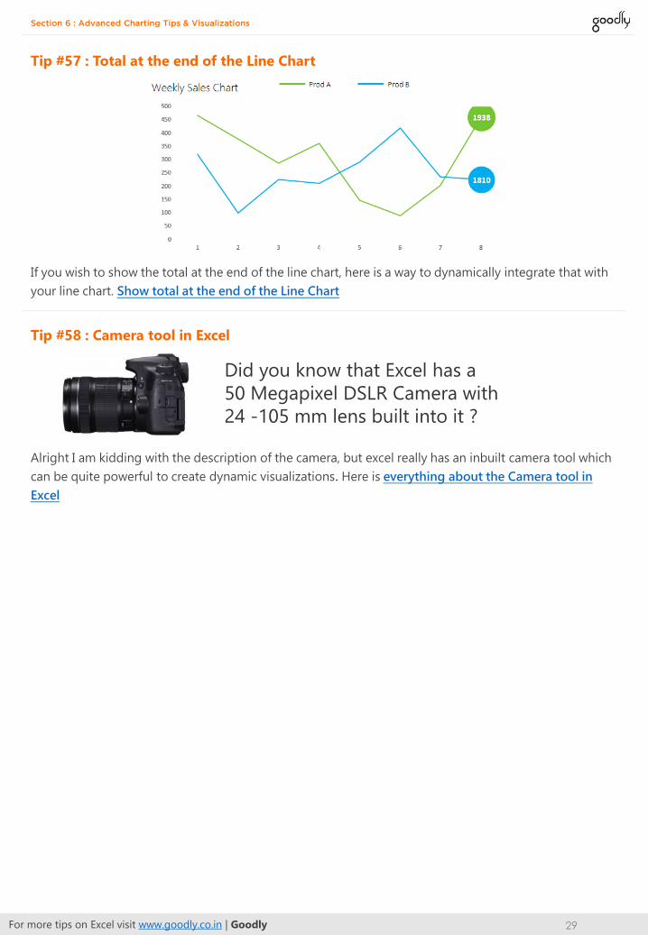
Tip #57 : Total at the end of the Line Chart

If you wish to show the total at the end of the line chart, here is a way to dynamically integrate that with

your line chart. Show total at the end of the Line Chart

Tip #58 : Camera tool in Excel

Did you know that Excel has a

50 Megapixel DSLR Camera with

24 -105 mm lens built into it ?

Alright I am kidding with the description of the camera, but excel really has an inbuilt camera tool which

can be quite powerful to create dynamic visualizations. Here is everything about the Camera tool in

Excel

For more tips on Excel visit www.goodly.co.in | Goodly 30

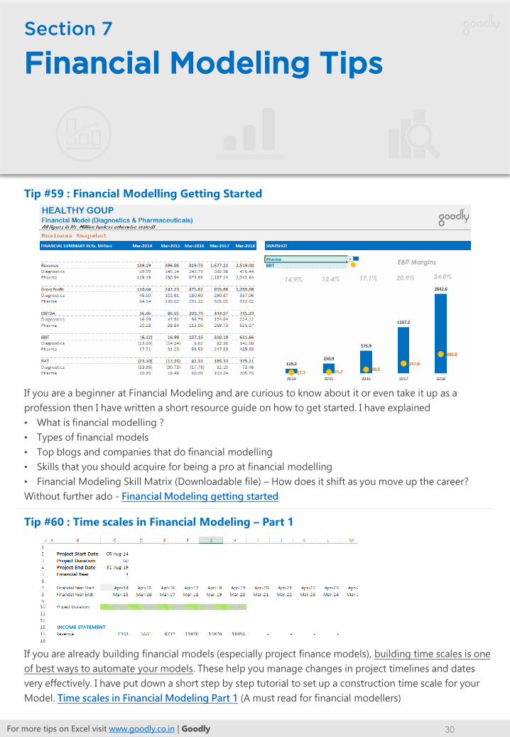
Section 7

Financial Modeling Tips

Tip #59 : Financial Modelling Getting Started

If you are a beginner at Financial Modeling and are curious to know about it or even take it up as a

profession then I have written a short resource guide on how to get started. I have explained

• What is financial modelling ?

• Types of financial models

• Top blogs and companies that do financial modelling

• Skills that you should acquire for being a pro at financial modelling

• Financial Modeling Skill Matrix (Downloadable file) – How does it shift as you move up the career?

Without further ado - Financial Modeling getting started

Tip #60 : Time scales in Financial Modeling – Part 1

If you are already building financial models (especially project finance models), building time scales is one

of best ways to automate your models. These help you manage changes in project timelines and dates

very effectively. I have put down a short step by step tutorial to set up a construction time scale for your

Model. Time scales in Financial Modeling Part 1 (A must read for financial modellers)

For more tips on Excel visit www.goodly.co.in | Goodly 31

Section 7 : Financial Modeling Tips

Tip #61 : Time Scales in Financial Modeling Part 2

This post is an extension of the Part 1 post on time scales with the difference being that this one is on

building project execution days. Read the entire post here – Time Scales in Financial Modeling Part 2

Tip #62 : IRR Calculation in Excel (1st Part)

What is IRR?

A lot of people will give life threating definitions of this concept! Definitions that they themselves hardly

understand, let alone using it practically in real life.

If you would like to understand the concept of IRR in a more human way and how it applies to real life you

must read this post. I have also charted out different problems associated with using IRR and their

workarounds

IRR Part 1 - Part 1 – Contents

1. What is IRR ? (A complex and a simple definition)

2. A Case to explain the concept of IRR

3. How to Calculate IRR (Simple math equation and by using Excel’s IRR function)

4. Investing or Not Investing in the Business (Case Analysis)

5. Interpreting Positive and Negative IRR

IRR Part 2 – Part 2 Contents

1. 4 problems associated with IRR

2. The XIRR function to handle irregular cash flows

3. Why does IRR change when consolidating annual cash flows from quarterly cash flows ?

4. Why is IRR or XIRR is not a very robust metric ?

IRR Part 3 – Part 3 Contents

Talks about Excel’s MIRR (modified internal rate of return) as a robust alternative to IRR

Tip #63 : IRR Calculation in Excel (2nd Part)

Tip #64 : IRR Calculation in Excel (3rd Part)

For more tips on Excel visit www.goodly.co.in | Goodly 32

Section 8

Miscellaneous Utility Tools

Tip #65 : Screen Editing Options in Excel

Excel offers additional capability to change the user interface. In this article I am covering 9 screen editing

options that offer the most utility to the user. 9 quick screen editing options in Excel

Tip #66 : How Goal Seek Works ?

Goal seek is one of the incredibly simple (& powerful) features of excel. It offers reverse one variable

analysis, something like : you know the result that you want but want to back calculate the variables for

the desired result. Take a look at a Case Study for Goal Seek

For more tips on Excel visit www.goodly.co.in | Goodly 33

Section 8 : Miscellaneous Utility Tools

Tip #67 : An alternative to merging cells

Cells are merged here !

We often merge the cells for a common headline that has to appear above a set of cells. There is a smart

way gives you the merge effect without merging the cells

Center Across Selection

1. Select the cells that you want to merge

2. Open the format cells box (shortcut Ctrl + 1)

3. In the alignment tab

4. Pick Center Across Selection

5. Done!

Now your cells will look like merged but actually the text is aligned to the center of the selected cells

1

2

3

4

For more tips on Excel visit www.goodly.co.in | Goodly 34

Section 8 : Miscellaneous Utility Tools

Tip #68 : Hiding Options in Excel

Excel offers quite a bit of hiding options by using them you can hide sheet tabs, ribbons, gridlines and

even the data. Here are 9 things you can choose to hide (and unhide) in Excel

Tip #70 : Protected sheet from being edited

If you wish to guard your sheet from unwanted access, the Protect Sheet feature comes really handy! I

have covered this in detail here – Sheet Protection Options in Excel

Tip #71 : Hyperlinking Options in Excel

I strongly recommend this utility for making your spreadsheets look more

aesthetically appealing. Here is how we do it

1. Click on shapes in the insert column, choose the rectangle tool and draw a

rectangle

2. Type a relevant message in the box and then right click on the box to choose the

hyperlink option

1

For more tips on Excel visit www.goodly.co.in | Goodly 35

Section 8 : Miscellaneous Utility Tools

3. The hyperlink dialogue box gives you the option for linking your object (rectangle) to same or any

other spreadsheet. You can even choose link a url (a website) to the object. Hyperlinking works on almost

anything- Objects, Pictures, Text, SmartArt

2

3

Tip #72 : Open the same Excel file multiple times with New Window Tool

Have you had a chance where you had a to do a lot of to and fro between sheets? If yes then the ‘New

Window’ feature is your saviour! It is an awesome tool for tracking workbooks with too many sheets

1. The New Window option is in the view tab

2. When you click on it, it opens up another image of your workbook in separate window and allows you

to refer to the sheets within your workbook from another window

For a single workbook you can open as many newwindows as you want

For more tips on Excel visit www.goodly.co.in | Goodly 36

Section 8 : Miscellaneous Utility Tools

3. Note that the new windows are mirror images and any changes done in the current window are

automatically updated in the file

4. This feature helps you compare a workbook with many sheets at one go (by using Alt+tab), rather than

navigating to and fro between sheets

Tip #73 : Working on Multiple Sheets

This trick really comes handy when you have to add data / edit multiple sheets at once. Let’s just take a

look into this, it is quick and easy! How to work on Multiple Sheets at once

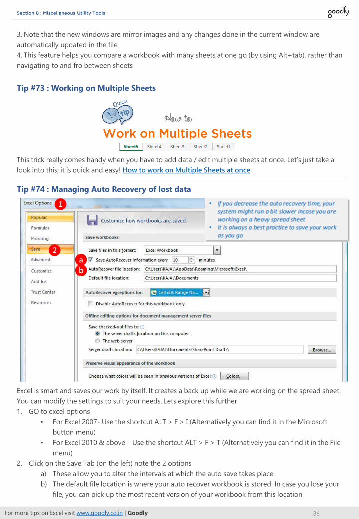
Tip #74 : Managing Auto Recovery of lost data

Excel is smart and saves our work by itself. It creates a back up while we are working on the spread sheet.

You can modify the settings to suit your needs. Lets explore this further

1. GO to excel options

• For Excel 2007- Use the shortcut ALT > F > I (Alternatively you can find it in the Microsoft

button menu)

• For Excel 2010 & above – Use the shortcut ALT > F > T (Alternatively you can find it in the File

menu)

2. Click on the Save Tab (on the left) note the 2 options

a) These allow you to alter the intervals at which the auto save takes place

b) The default file location is where your auto recover workbook is stored. In case you lose your

file, you can pick up the most recent version of your workbook from this location

1

2

a

b

For more tips on Excel visit www.goodly.co.in | Goodly 37

Section 8 : Miscellaneous Utility Tools

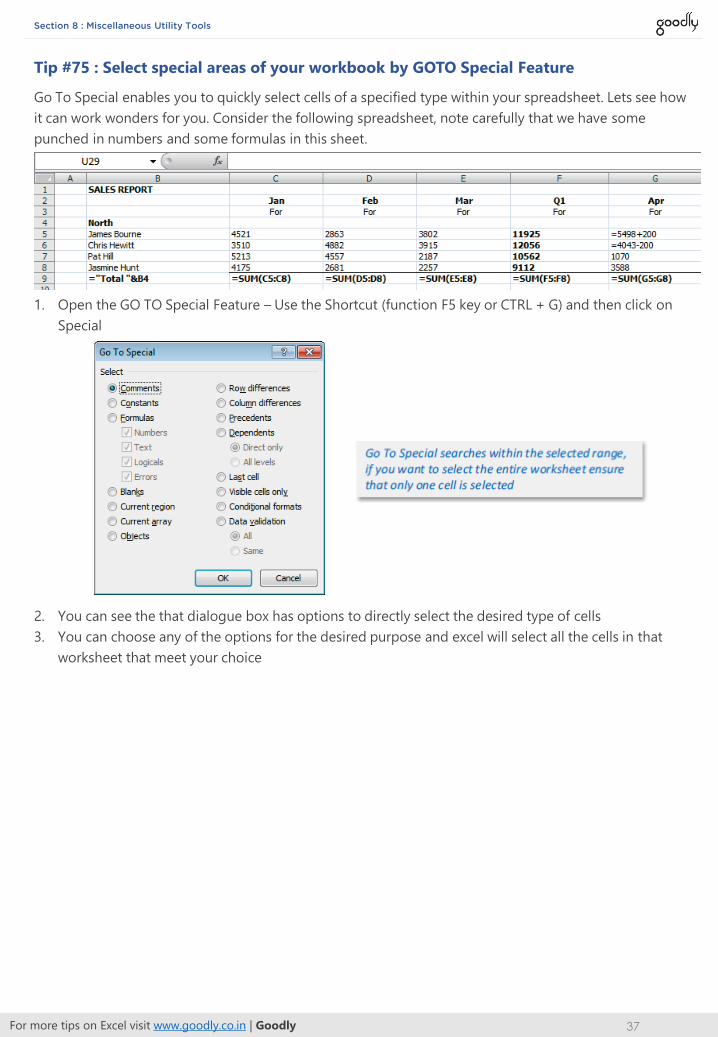
Tip #75 : Select special areas of your workbook by GOTO Special Feature

Go To Special enables you to quickly select cells of a specified type within your spreadsheet. Lets see how

it can work wonders for you. Consider the following spreadsheet, note carefully that we have some

punched in numbers and some formulas in this sheet.

1. Open the GO TO Special Feature – Use the Shortcut (function F5 key or CTRL + G) and then click on

Special

2. You can see the that dialogue box has options to directly select the desired type of cells

3. You can choose any of the options for the desired purpose and excel will select all the cells in that

worksheet that meet your choice

For more tips on Excel visit www.goodly.co.in | Goodly 38

Section 8 : Miscellaneous Utility Tools

Tip #76 : Customizing Ribbon to suit your needs

Excel 2010 & above versions have gone a step further to make working on excel convenient for you.

Customizing ribbon allows you to add a Tab with tools and buttons of your own choice. Check this out

1. When you click New Tab, you can add a custom tab and custom group. You can only add commands

to custom groups

2. To rename a tab, click the tab that you want to rename and click Rename

For more tips on Excel visit www.goodly.co.in | Goodly 39

Section 9

VBA Automation & Quick Resources

Tip #77 : 60 VBA Shortcuts

Tip #78 : Consolidate Data from Multiple Sheets

I have put together a list 60+ VBA Shortcuts that will boost your speed and productivity while using VBA.

Be it editing the code, debugging it, navigating the VB window or accessing far off options in the menu

bar.. its all in here. 60+ VBA Shortcuts

One of the common problems in managing data is bringing it all together. Let’s say we have some data

scattered in multiple sheets that we want to bring it together in a single sheet. How would you do it?

One way is to copy it from multiple sheets and paste it at one location or the smarter was is to write a

simple macro to do the same for us.

Here is a short VBA code that will help you Consolidate data from multiple sheets

For more tips on Excel visit www.goodly.co.in | Goodly 40

Section 9 : VBA Automation & Quick Resources

Tip #79 : Create an Index from Sheet Names in Excel

If you have multiple sheets in your workbook and you would like to create an Index Sheet with

hyperlinked names to all the sheets, here is smart and quick way to do it with a short macro code. Create

a sheet index in Excel

Tip #80 : Covert numbers into Indian Currency Words

This is one of the top request from accountants : How can I convert numbers into words. There is not a

straight way to do it but a macro. The code is pretty complex but you need not worry, all you have got to

do is to copy and paste the code and that’s it

Get my step by step instruction here – Convert numbers into Indian Currency Words

Excel can hide multiple sheets at a time but cannot unhide all of them at one go and it gets quite irritating

at times. Here is short code to make you rid of the itchy feeling while unhiding sheets :D

Unhide all Sheets at Once

Tip #81 (Bonus Tip) : Unhiding Multiple Sheets at Once

Share this E BookThank you for reading…I hope you enjoyed reading this EBook!

I encourage you to write to me for any excel questions or even if you would like to drop in a “hi” on

goodly.wordpress@gmail.com, I will be more than happy to help you in the best way I can. Also do not

forget to send this eBook to your friends who need it!

Cheers & stay tuned to Goodly

Chandeep

www.goodly.co.in