excel using excel
TRANSCRIPT

8/7/2019 Excel using Excel
http://slidepdf.com/reader/full/excel-using-excel 1/61

8/7/2019 Excel using Excel
http://slidepdf.com/reader/full/excel-using-excel 2/61
About Excel
Tool developed by Microsoft Corporation
Consists of Rows and Columns - Cells
Create, Format, Sort and Analyze data
Spreadsheets, Tables & Statements
Graphical Representation
Automatic Recalculation ± Saves time &effort

8/7/2019 Excel using Excel
http://slidepdf.com/reader/full/excel-using-excel 3/61
Components of the Excel Window
Microsoft Office Button
Quick Access Toolbar
Title Bar
Ribbon Tabs & Ribbon, Galleries & Tools
Name Box
Formula Bar Worksheet
Status Bar

8/7/2019 Excel using Excel
http://slidepdf.com/reader/full/excel-using-excel 4/61
Microsoft
Office
Button
Quick Access Toolbar The Title Bar

8/7/2019 Excel using Excel
http://slidepdf.com/reader/full/excel-using-excel 5/61
The Microsoft Office Button
In the upper-left corner of the Excel 2007 window is the Microsoft Office button. When
you click the button, a menu appears. You can use the menu to create a new file, open
an existing file, save a file, and perform many other tasks.
The Quick Access Toolbar Next to the Microsoft Office button is the Quick Access toolbar. The Quick Access toolbar
gives you with access to commands you frequently use. By default, Save, Undo, and
Redo appear on the Quick Access toolbar. You can use Save to save your file, Undo to
roll back an action you have taken, and Redo to reapply an action you have rolled back.
The Title Bar Next to the Quick Access toolbar is the Title bar. On the Title bar, Microsoft Excel
displays the name of the workbook you are currently using. At the top of the Excel
window, you should see "Microsoft Excel - Book1" or a similar name

8/7/2019 Excel using Excel
http://slidepdf.com/reader/full/excel-using-excel 6/61
The Ribbon
You use commands to tell Microsoft Excel what to do. In Microsoft Excel 2007, you use
the Ribbon to issue commands. The Ribbon is located near the top of the Excel window,
below the Quick Access toolbar. At the top of the Ribbon are several tabs; clicking a tab
displays several related command groups. Within each group are related command
buttons. You click buttons to issue commands or to access menus and dialog boxes. You
may also find a dialog box launcher in the bottom-right corner of a group. When you click
the dialog box launcher, a dialog box makes additional commands available.

8/7/2019 Excel using Excel
http://slidepdf.com/reader/full/excel-using-excel 7/61
Worksheets Microsoft Excel consists of
worksheets.
Each worksheet contains columnsand rows.
The columns are 16384 lettered A to
Z and then continuing with AA, AB,
AC and so on;
the rows are numbered 1 to
1,048,576.
The number of columns and rows
you can have in a worksheet is
limited by your computer memor y
and your system resources.
The combination of a column
coordinate and a row coordinate
make up a cell address.
For example, the cell located in the
upper-left corner of the worksheet is
cell A1, meaning column A, row 1.
Cell E10 is located under column E
on row 10. You enter your data into
the cells on the worksheet.
8/7/2019 Excel using Excel
http://slidepdf.com/reader/full/excel-using-excel 8/61
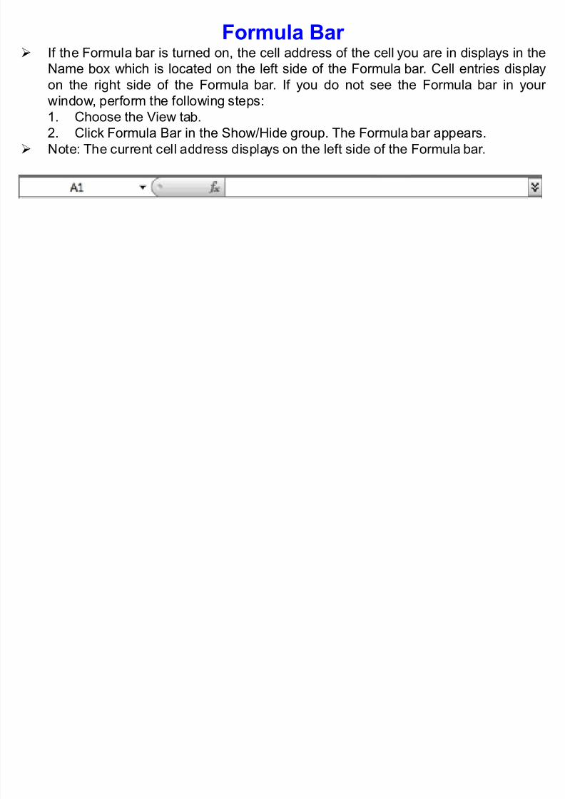
Formula Bar If the Formula bar is turned on, the cell address of the cell you are in displays in the
Name box which is located on the left side of the Formula bar. Cell entries display
on the right side of the Formula bar. If you do not see the Formula bar in your
window, perform the following steps:1. Choose the View tab.
2. Click Formula Bar in the Show/Hide group. The Formula bar appears.
Note: The current cell address displays on the left side of the Formula bar.

8/7/2019 Excel using Excel
http://slidepdf.com/reader/full/excel-using-excel 9/61
The Status Bar The Status bar appears
at the ver y bottom of the
Excel window and
provides suchinformation as the sum,
average, minimum, and
maximum value of
selected numbers. You
can change what
displays on the Statusbar by right-clicking on
the Status bar and
selecting the options you
want from the Customize
Status Bar menu. You
click a menu item toselect it. You click it
again to deselect it. A
check mark next to an
item means the item is
selected

8/7/2019 Excel using Excel
http://slidepdf.com/reader/full/excel-using-excel 10/61
8/7/2019 Excel using Excel
http://slidepdf.com/reader/full/excel-using-excel 11/61
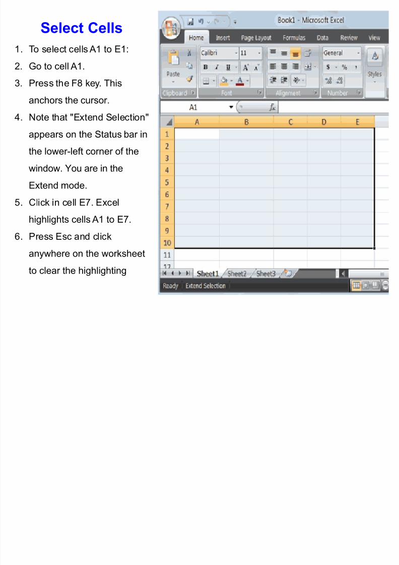
Select Cells
1. To select cells A1 to E1:
2. Go to cell A1.3. Press the F8 key. This
anchors the cursor.
4. Note that "Extend Selection"
appears on the Status bar in
the lower-left corner of the
window. You are in the
Extend mode.
5. Click in cell E7. Excel
highlights cells A1 to E7.
6. Press Esc and click
anywhere on the worksheet
to clear the highlighting

8/7/2019 Excel using Excel
http://slidepdf.com/reader/full/excel-using-excel 12/61
Enter Data1. The cursor in cell A1.
2. Type John Jordan. Do not press Enter at
this time.
Delete Data1. The Backspace key erases one
character at a time.2. Press the Backspace key until Jordan is
erased.
3. Press Enter. The name "John" appears
in cell A1.

8/7/2019 Excel using Excel
http://slidepdf.com/reader/full/excel-using-excel 13/61
Edit a Cell1. After you enter data into a cell, you can
edit the data by pressing F2 while you
are in the cell you wish to edit.

8/7/2019 Excel using Excel
http://slidepdf.com/reader/full/excel-using-excel 14/61
Editing a Cell by
Using the Formula
Bar 1. Move the cursor to cell A1.2. Click in the formula area of the
Formula bar
3. Use the backspace key to
erase the "s," "e," and "n.³
4. Type ker.
5. Press Enter.
8/7/2019 Excel using Excel
http://slidepdf.com/reader/full/excel-using-excel 15/61
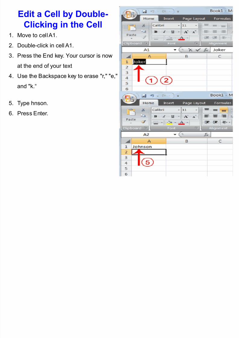
Edit a Cell by Double-
Clicking in the Cell1. Move to cell A1.
2. Double-click in cell A1.
3. Press the End key. Your cursor is now
at the end of your text
4. Use the Backspace key to erase "r," "e,"
and "k.³
5. Type hnson.
6. Press Enter.

8/7/2019 Excel using Excel
http://slidepdf.com/reader/full/excel-using-excel 16/61
Change the Cell Entry
Wrap Text Tool1. Change a Cell Entr y
2. Typing in a cell replaces the old cell
entr y with the new information you type.
3. Move the cursor to cell A1.
4. Type Cathy.
5. Press Enter. The name "Cathy"
replaces "Johnson
6. Move to cell A2.
7. Type Text too long to fit.
8. Press Enter.
9. Return to cell A2.
10.Choose the Home tab.
11.Click the Wrap Text button . Excel
wraps the text in the cell.

8/7/2019 Excel using Excel
http://slidepdf.com/reader/full/excel-using-excel 17/61
1. Click the Microsoft Office button. A
menu appears.
2. Click Excel Options in the lower-right
corner. The Excel Options pane
appears.
3. Click Advanced.
4. If the check box next to After Pressing
Enter Move Selection is not checked,
click the box to check it.
5. If Down does not appear in the
Direction box, click the down arrow
next to the Direction box and then click
Down.
6. Click OK. Excel sets the Enter
direction to down.
Change the Cell Entry Direction

8/7/2019 Excel using Excel
http://slidepdf.com/reader/full/excel-using-excel 18/61
Mathematical Calculations you can enter numbers and mathematical formulas into cells.
Whether you enter a number or a formula, you can reference the cell when you
perform mathematical calculations such as addition, subtraction, multiplication, or
division.
When entering a mathematical formula, precede the formula with an equal sign.
Use the following to indicate the type of calculation you wish to perform
+ Addition
- Subtraction
* Multiplication
/ Division
^ Exponential
8/7/2019 Excel using Excel
http://slidepdf.com/reader/full/excel-using-excel 19/61
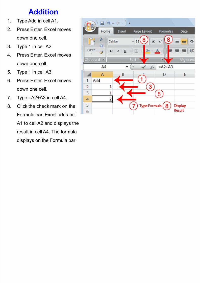
Addition1. Type Add in cell A1.
2. Press Enter. Excel moves
down one cell.
3. Type 1 in cell A2.
4. Press Enter. Excel moves
down one cell.
5. Type 1 in cell A3.
6. Press Enter. Excel moves
down one cell.
7. Type = A2+ A3 in cell A4.
8. Click the check mark on the
Formula bar. Excel adds cell
A1 to cell A2 and displays the
result in cell A4. The formula
displays on the Formula bar

8/7/2019 Excel using Excel
http://slidepdf.com/reader/full/excel-using-excel 20/61
Subtraction4. Type Subtract.
5. Press Enter.
Excel moves down one cell.
6. Type 6 in cell B2.
7. Press Enter.
Excel moves down one cell.
8. Type 3 in cell B3.
9. Press Enter.
Excel moves down one cell.
10. Type =B2-B3 in cell B4.
11. Click the check mark on
Formula bar. Excel subtracts
cell B3 from cell B2 & the result
displays in cell B4. The formula
displays on Formula bar.

8/7/2019 Excel using Excel
http://slidepdf.com/reader/full/excel-using-excel 21/61
Automatic Calculation1. Move to cell A2.
2. Type 2.
3. Press the right arrow key. Excel
changes the result in cell A4. Excel
adds cell A2 to cell A3 and the new
result appears in cell A4.
4. Move to cell B2.
5. Type 8.
6. Press the right arrow key. Excel
subtracts cell B3 from cell B3 and
the new result appears in cell B4.
7. Move to cell C2.
8. Type 4.
9. Press the right arrow key. Excel
multiplies cell C2 by cell C3 and thenew result appears in cell C4.
10. Move to cell D2.
11. Type 12.
12. Press the Enter key. Excel divides
cell D2 by cell D3 and the new result
appears in cell D4

8/7/2019 Excel using Excel
http://slidepdf.com/reader/full/excel-using-excel 22/61
Math Rule1. Move to cell A7.
2. Type =3+3+12/2*4.
3. Press Enter.
4. Note: Microsoft Excel divides 12 by 2, multiplies the answer by 4, adds 3, and thenadds another 3. The answer, 30, displays in cell A7
Math Rule1. Double-click in cell A7.
2. Edit the cell to read =(3+3+12)/2*4.
3. Press Enter.
4. Note: Microsoft Excel adds 3 plus 3 plus 12, divides the answer by 2, and thenmultiplies the result by 4. The answer, 36, displays in cell A7.
3+3+12*4
2

8/7/2019 Excel using Excel
http://slidepdf.com/reader/full/excel-using-excel 23/61
Align Cell Entries
Centre1. Select cells A1 to D1.
2. Choose the Home tab.
3. Click the Center button in
the Alignment group. Excel
centers each cell's content
Align Cell Entries
Left1. Select cells A1 to D1.
2. Choose the Home tab.
3. Click the Align Text Left button
in the Alignment group. Excel
left-aligns each cell's content

8/7/2019 Excel using Excel
http://slidepdf.com/reader/full/excel-using-excel 24/61
Copy - Paste
Ribbon
1. You should be in cell A12.2. Choose the Home tab.
3. Click the Copy button in the
Clipboard group. Excel copies
the formula in cell A12
4. Press the right arrow key once
to move to cell B12.
5. Click the Paste button in the
Clipboard group. Excel pastes
the formula in cell A12 into cell
B12.
6. Press the Esc key to exit the
Copy mode

8/7/2019 Excel using Excel
http://slidepdf.com/reader/full/excel-using-excel 25/61
Copy - PasteMini Toolbar
1. Select cells A9 to B11. Move to
cell A9. Press the Shift key.
While holding down the Shift
key, press the down arrow key
twice. Press the right arrow key
once. Excel highlights A9 to B11.
2. Right-click. A context menu and
a Mini toolbar appear.
3. Click Copy, which is located on
the context menu. Excel copiesthe information in cells A9 to B1

8/7/2019 Excel using Excel
http://slidepdf.com/reader/full/excel-using-excel 26/61
Cut - Paste
1. Select cells D9 to
D12
2. Choose the Home
tab.
3. Click the Cut button.
4. Move to cell G1
5. Click the Paste
button .
6. Excel moves the
contents of cells D9
to D12 to cells G1 to
G4

8/7/2019 Excel using Excel
http://slidepdf.com/reader/full/excel-using-excel 27/61
Cut - Paste
1. Select cells D9 toD12
2. Choose the Home
tab.
3. Click the Cut button.
4. Move to cell G1
5. Click the Paste
button .
6. Excel moves the
contents of cells D9
to D12 to cells G1 to
G4
8/7/2019 Excel using Excel
http://slidepdf.com/reader/full/excel-using-excel 28/61
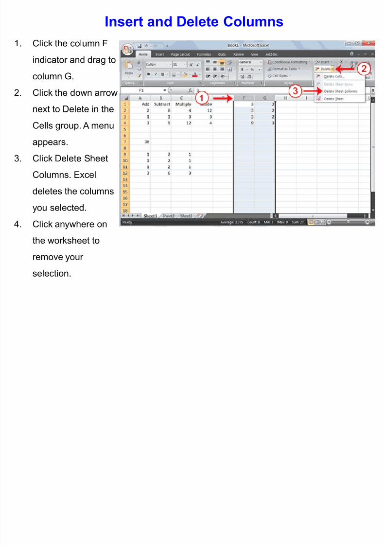
Insert and Delete Columns
1. Click the column F
indicator and drag to
column G.
2. Click the down arrow
next to Delete in the
Cells group. A menu
appears.
3. Click Delete Sheet
Columns. Excel
deletes the columns
you selected.
4. Click anywhere on
the worksheet to
remove your
selection.

8/7/2019 Excel using Excel
http://slidepdf.com/reader/full/excel-using-excel 29/61
Insert and Delete Rows1. Click the row 7 indicator and drag to row 12.
2. Click the down arrow next to Delete in the Cells group. A menu appears.
3. Click Delete Sheet Rows. Excel deletes the rows you selected.
4. Click anywhere on the worksheet to remove your selection

8/7/2019 Excel using Excel
http://slidepdf.com/reader/full/excel-using-excel 30/61
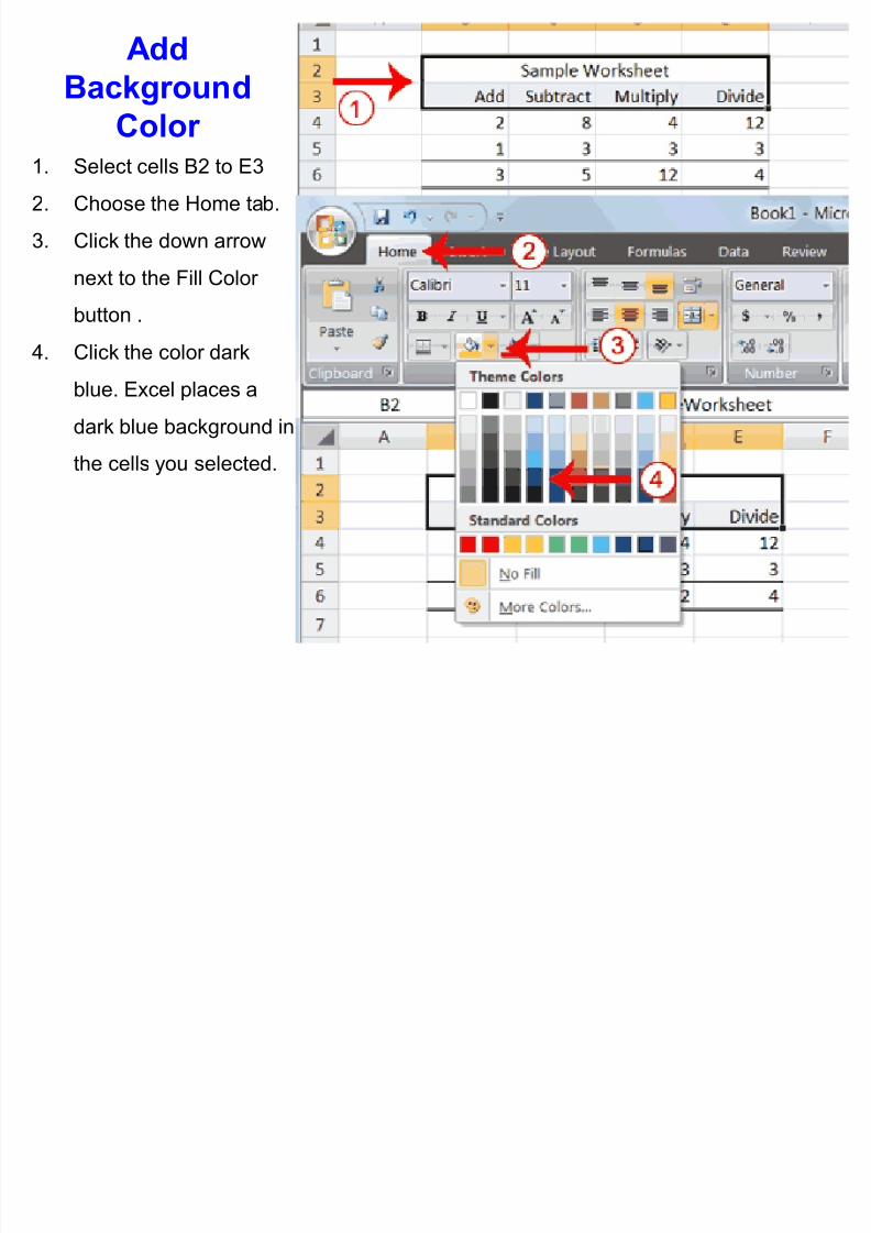
Create Bor ders
1. Select cells B6 to E6
2. Choose the Home tab.
3. Click the down arrow next to theBorders button . A menu appears.
4. Click Top and Double Bottom Border.
Excel adds the border you chose to
the selected cells

8/7/2019 Excel using Excel
http://slidepdf.com/reader/full/excel-using-excel 31/61
Merge & Centre1. Go to cell B2.
2. Type Sample Worksheet.
3. Click the check mark on the Formula bar.
4. Select cells B2 to E2.5. Choose the Home tab.
6. Click the Merge and Center button in the Alignment group. Excel merges cells B2,
C2, D2, and E2 and then centers the content
8/7/2019 Excel using Excel
http://slidepdf.com/reader/full/excel-using-excel 32/61
8/7/2019 Excel using Excel
http://slidepdf.com/reader/full/excel-using-excel 33/61
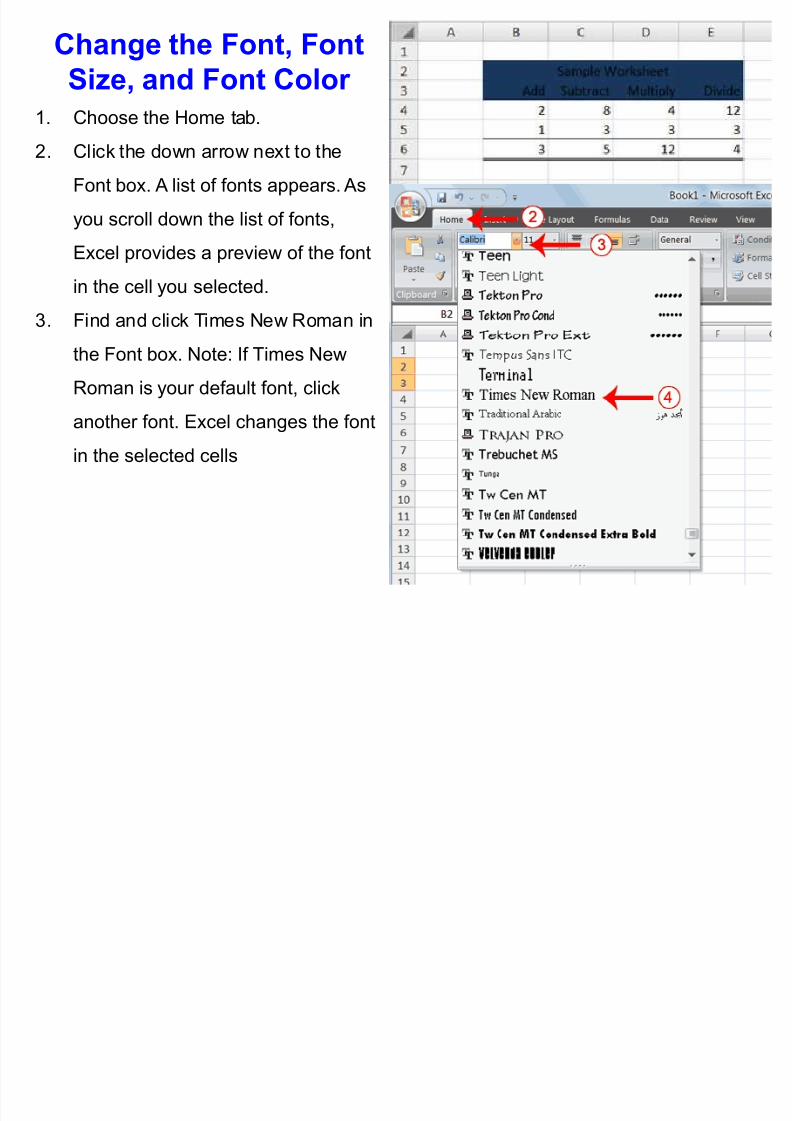
1. Choose the Home tab.
2. Click the down arrow next to the
Font box. A list of fonts appears. As
you scroll down the list of fonts,
Excel provides a preview of the font
in the cell you selected.
3. Find and click Times New Roman in
the Font box. Note: If Times New
Roman is your default font, click
another font. Excel changes the font
in the selected cells
Change the Font, Font
Size, and Font Color

8/7/2019 Excel using Excel
http://slidepdf.com/reader/full/excel-using-excel 34/61
Change the
Font Size1. Select cell B2.
2. Choose the Home
tab.
3. Click the down arrow
next to the Font Size
box. A list of font sizesappears. As you scroll
up or down the list of
font sizes, Excel
provides a preview of
the font size in the
cell you selected.
4. Click 26. Excel
changes the font size
in cell B2 to 26
8/7/2019 Excel using Excel
http://slidepdf.com/reader/full/excel-using-excel 35/61
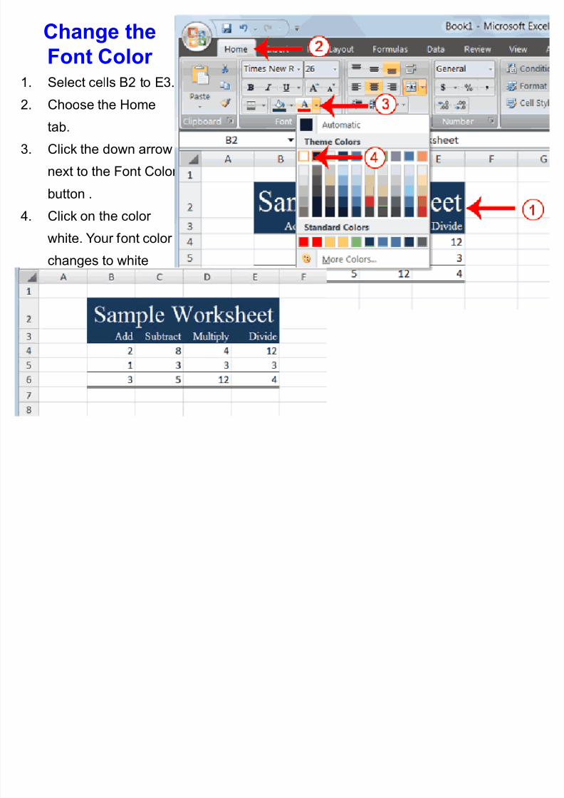
Change the
Font Color 1. Select cells B2 to E3.
2. Choose the Home
tab.
3. Click the down arrow
next to the Font Color
button .4. Click on the color
white. Your font color
changes to white
8/7/2019 Excel using Excel
http://slidepdf.com/reader/full/excel-using-excel 36/61
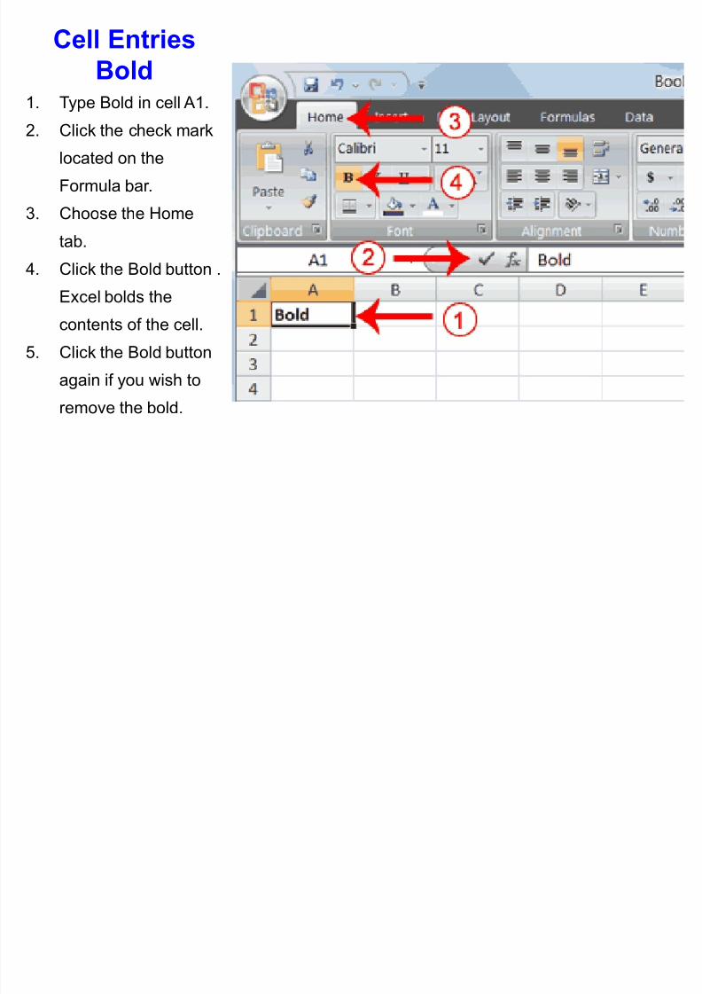
Cell Entries
Bold1. Type Bold in cell A1.
2. Click the check mark
located on the
Formula bar.
3. Choose the Home
tab.4. Click the Bold button .
Excel bolds the
contents of the cell.
5. Click the Bold button
again if you wish to
remove the bold.

8/7/2019 Excel using Excel
http://slidepdf.com/reader/full/excel-using-excel 37/61
Cell Entries Italic
1. Type Italic in cell B1.
2. Click the check mark
located on the
Formula bar.
3. Choose the Home
tab.4. Click the Italic button .
Excel italicizes the
contents of the cell.
5. Click the Italic button
again if you wish to
remove the italic
8/7/2019 Excel using Excel
http://slidepdf.com/reader/full/excel-using-excel 38/61
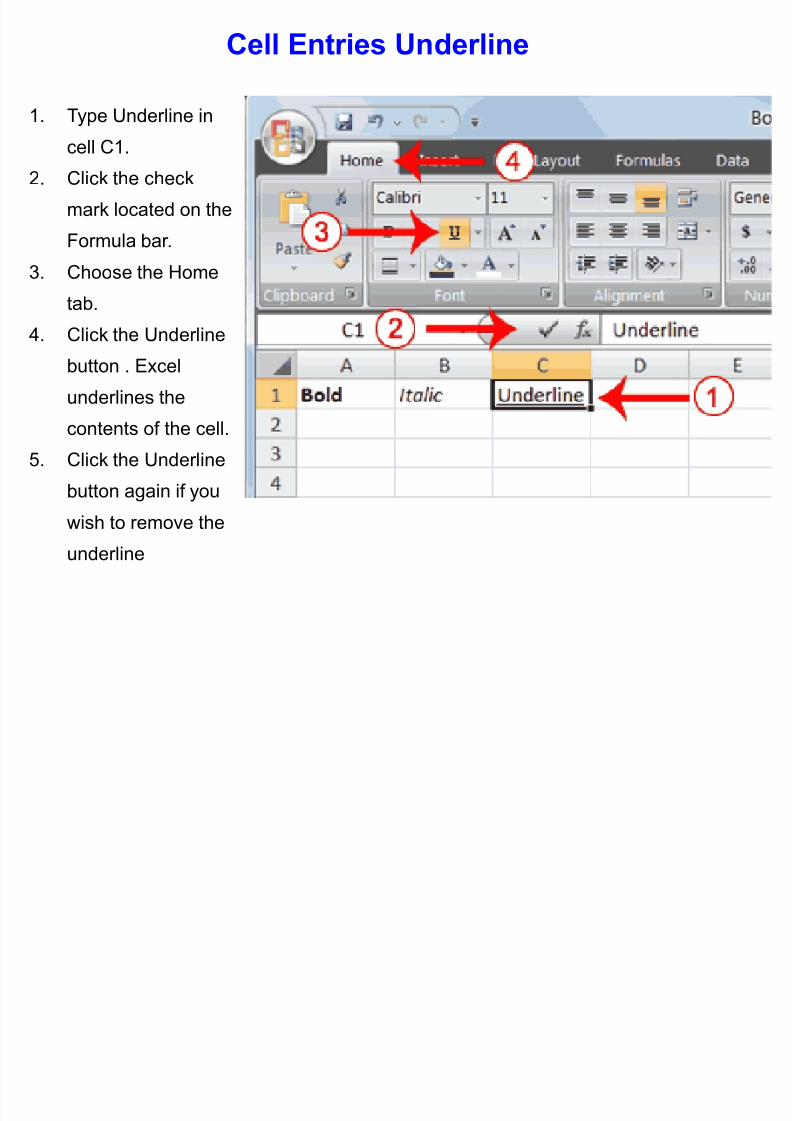
Cell Entries Underline
1. Type Underline in
cell C1.
2. Click the check
mark located on the
Formula bar.
3. Choose the Hometab.
4. Click the Underline
button . Excel
underlines the
contents of the cell.
5. Click the Underline
button again if you
wish to remove the
underline

8/7/2019 Excel using Excel
http://slidepdf.com/reader/full/excel-using-excel 39/61
Cell Entries Double Underline
1. Type Underline in cell D1.
2. Click the check mark located on the Formula bar.
3. Choose the Home tab.
4. Click the double underline button again if you wish to remove the double underline

8/7/2019 Excel using Excel
http://slidepdf.com/reader/full/excel-using-excel 40/61
Column Width1. Choose the Home tab.
2. Click the down arrow next to Format in the Cells group.
3. Click Column Width. The Column Width dialog box appears.
4. Type 55 in the Column Width field.
5. Click OK. Column A is set to a width of 55. You should now be able to see all of the
text

8/7/2019 Excel using Excel
http://slidepdf.com/reader/full/excel-using-excel 41/61

8/7/2019 Excel using Excel
http://slidepdf.com/reader/full/excel-using-excel 42/61
Format Numbers7. Click the Comma Style button . Excel separates thousands with a comma.
8. Click the Accounting Number Format button . Excel adds a dollar sign to your
number.
9. Click twice on the Increase Decimal button to change the number format to four decimal places.
10. Click the Decrease Decimal button if you wish to decrease the number of
decimal places

8/7/2019 Excel using Excel
http://slidepdf.com/reader/full/excel-using-excel 43/61
Decimal to Percent
1. Move to cell B9.
2. Type .35 (note the decimal point).
3. Click the check mark on the
formula bar
4. Choose the Home tab.
5. Click the Percent Style button .
Excel turns the decimal to a
percent
1 Ch th I t t b

8/7/2019 Excel using Excel
http://slidepdf.com/reader/full/excel-using-excel 44/61
Header & Footer 1. Choose the Insert tab.
2. Click the Header & Footer button in the Text group. Your worksheet changes to
Page Layout view and the Design context tab appears. Note that your cursor is
located in the center section of the header area

8/7/2019 Excel using Excel
http://slidepdf.com/reader/full/excel-using-excel 45/61
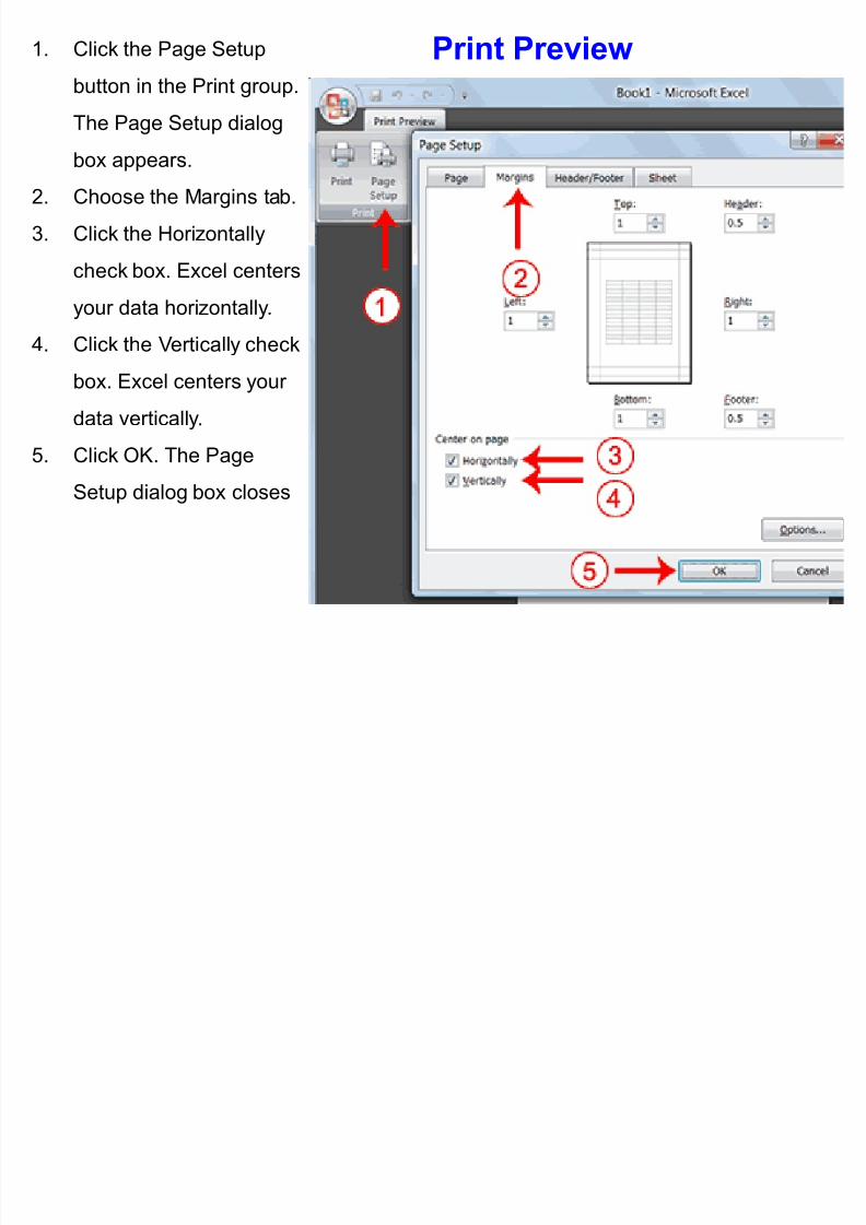
Page Layout1. Choose the Page
Layout tab.
2. Click Margins in the
Page Setup group. A
menu appears.3. Click Wide. Word sets
your margins to the
Wide settings

8/7/2019 Excel using Excel
http://slidepdf.com/reader/full/excel-using-excel 46/61
S P Si

8/7/2019 Excel using Excel
http://slidepdf.com/reader/full/excel-using-excel 47/61
Set Paper Size1. Choose the Page Layout
tab.
2. Click Size in the Page Setup
group. A menu appears.3. Click the paper size you are
using. Excel sets your page
size
P i t P i
8/7/2019 Excel using Excel
http://slidepdf.com/reader/full/excel-using-excel 48/61
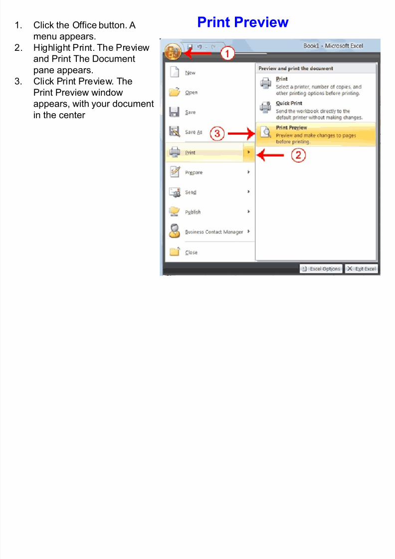
Print Preview1. Click the Office button. A
menu appears.
2. Highlight Print. The Preview
and Print The Document
pane appears.3. Click Print Preview. The
Print Preview window
appears, with your document
in the center
8/7/2019 Excel using Excel
http://slidepdf.com/reader/full/excel-using-excel 49/61
P i t
8/7/2019 Excel using Excel
http://slidepdf.com/reader/full/excel-using-excel 50/61
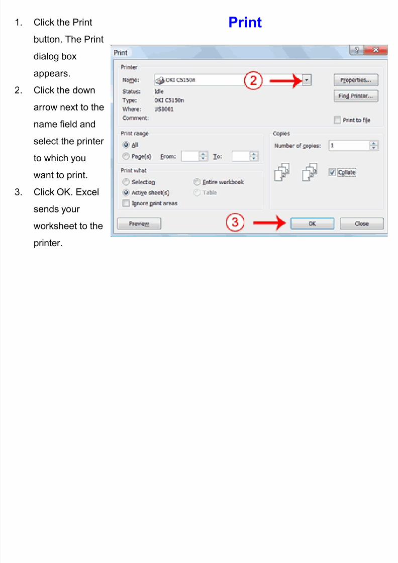
Print1. Click the Print
button. The Print
dialog box
appears.
2. Click the down
arrow next to the
name field and
select the printer
to which you
want to print.
3. Click OK. Excel
sends your worksheet to the
printer.
C ti Ch t

8/7/2019 Excel using Excel
http://slidepdf.com/reader/full/excel-using-excel 51/61
Creating Charts1. Select cells A3 to D6. You
must select all the cells
containing the data you
want in your chart. You
should also include the data
labels.
2. Choose the Insert tab.
3. Click the Column button in
the Charts group. A list of
column chart sub-types
types appears.
4. Click the Clustered Columnchart sub-type. Excel
creates a Clustered Column
chart and the Chart Tools
context tabs appear.
A l Ch t L t

8/7/2019 Excel using Excel
http://slidepdf.com/reader/full/excel-using-excel 52/61
Apply a Chart Layout1. Click your chart. The
Chart Tools become
available.
2. Choose the Design tab.
3. Click the Quick Layout
button in the Chart
Layout group. A list of
chart layouts appears.
4. Click Layout 5. Excel
applies the layout to
your chart
A l L b l1 S l t Ch t Titl Cli k Ch t
8/7/2019 Excel using Excel
http://slidepdf.com/reader/full/excel-using-excel 53/61
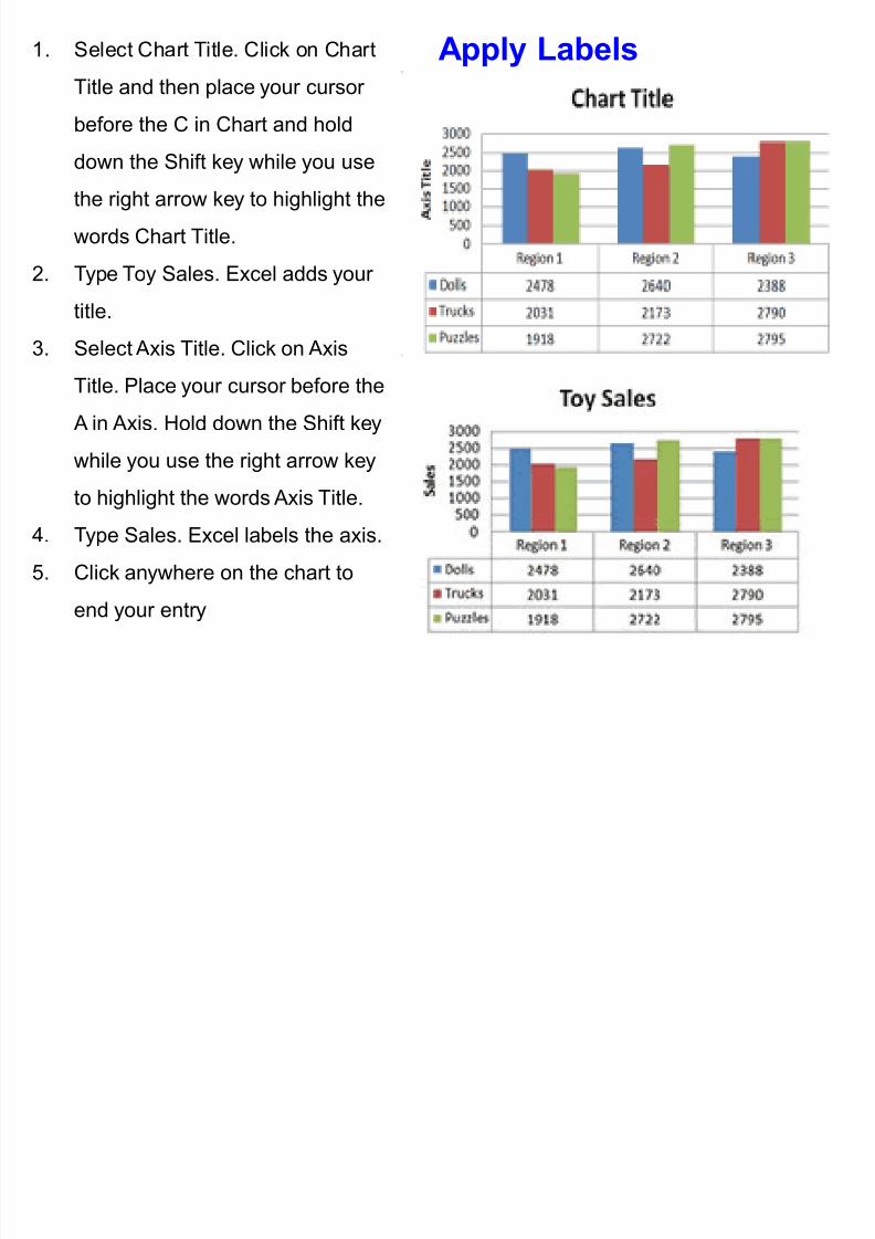
Apply Labels1. Select Chart Title. Click on Chart
Title and then place your cursor
before the C in Chart and hold
down the Shift key while you use
the right arrow key to highlight the
words Chart Title.
2. Type Toy Sales. Excel adds your
title.
3. Select Axis Title. Click on Axis
Title. Place your cursor before the
A in Axis. Hold down the Shift key
while you use the right arrow key to highlight the words Axis Title.
4. Type Sales. Excel labels the axis.
5. Click anywhere on the chart to
end your entr y
8/7/2019 Excel using Excel
http://slidepdf.com/reader/full/excel-using-excel 54/61
Change the Style of Charts

8/7/2019 Excel using Excel
http://slidepdf.com/reader/full/excel-using-excel 55/61
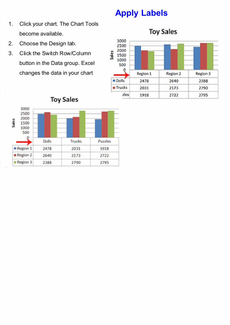
Change the Style of Charts1. Click your chart. The Chart Tools become available.
2. Choose the Design tab.
3. Click the More button in the Chart Styles group. The chart styles appear
4. Click Style 42. Excel applies the style to your chart.
Change the Style of Charts

8/7/2019 Excel using Excel
http://slidepdf.com/reader/full/excel-using-excel 56/61
Change the Style of Charts1. Click Style 42. Excel applies the style to your chart.
Change the Size and Position of Charts

8/7/2019 Excel using Excel
http://slidepdf.com/reader/full/excel-using-excel 57/61
Change the Size and Position of Charts
1. Use the handles to adjust the size of your chart.
2. Click an unused portion of the chart and drag to position the chart beside the data
Move a Chart to a Chart Sheet1 Click your chart

8/7/2019 Excel using Excel
http://slidepdf.com/reader/full/excel-using-excel 58/61
Move a Chart to a Chart Sheet1. Click your chart.
The Chart Tools
become
available.
2. Choose the
Design tab.3. Click the Move
Chart button in
the Location
group. The
Move Chart
dialog boxappears
4. Click the New
Sheet radio
button.
5. Type Toy Sales
to name thechart sheet.
Excel creates a
chart sheet
named Toy
Sales and
places your chart on it.
Functions
8/7/2019 Excel using Excel
http://slidepdf.com/reader/full/excel-using-excel 59/61
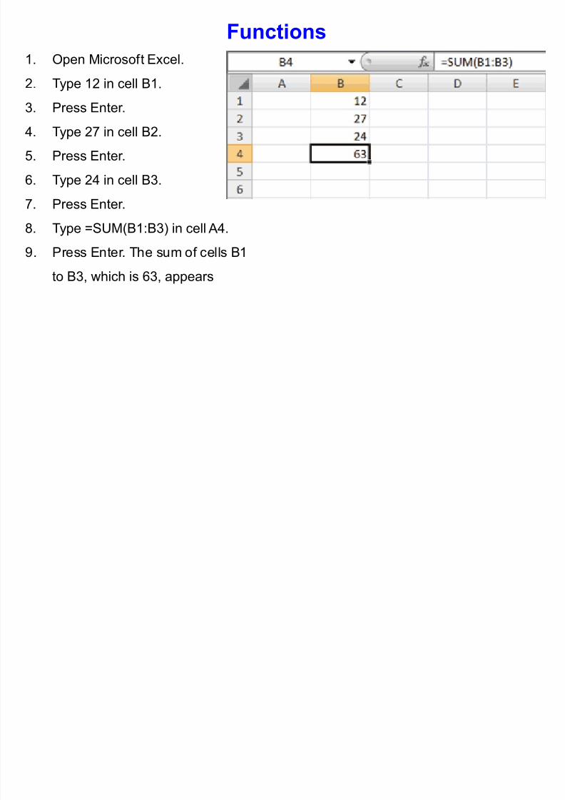
Functions
1. Open Microsoft Excel.
2. Type 12 in cell B1.
3. Press Enter.
4. Type 27 in cell B2.
5. Press Enter.
6. Type 24 in cell B3.
7. Press Enter.
8. Type =SUM(B1:B3) in cell A4.
9. Press Enter. The sum of cells B1
to B3, which is 63, appears
Applying Functions using Ribbon

8/7/2019 Excel using Excel
http://slidepdf.com/reader/full/excel-using-excel 60/61
Applying Functions using Ribbon

8/7/2019 Excel using Excel
http://slidepdf.com/reader/full/excel-using-excel 61/61
Cell Reference & Range Name
Absolute Reference & Mixed Reference
Create a Range Name: Name Box & Define Name
Functions: IF, Nested, AND, OR, NOT
VLOOKUP
Pivot Table