Excess Demand And Equilibration In Multi-Security Financial Markets:

The Empirical Evidence

Elena Asparouhova‡, Peter Bossaerts§ and Charles Plott¶

18 April 2002

Abstract: Price dynamics are studied in a dataset of more than 11,000 transactions from large-scale financial markets experiments

with multiple risky securities. The aim is to determine whether a few simple principles govern equilibration. We first ask whether

price changes are driven by excess demand. The data strongly support this conjecture. Second, we investigate the presence of

cross-security effects (the excess demands of other securities influence price changes of a security beyond its own excess demand).

We find systematic cross-security effects, despite the fact that transactions in one market cannot be made conditional on events

in other markets. Nevertheless, stability is not found to be compromised in our data. A curious relationship emerges between

the signs of the cross-effects and the signs of the covariances of the payoffs of the corresponding securities. It suggests a link

between price discovery in real markets and the Newton procedure in numerical computation of general equilibrium. Next, we

investigate whether the book (the set of posted limit orders) plays a role in the process by which excess demand becomes reflected

in transaction price changes. We find strong correlation between excess demands and a weighted average of the quotes in the

book. The correlation is far from perfect, and we document that our weighted average of the quotes in the book explains part of

the variance of transaction price changes that is unaccounted for by excess demands.

Keywords: Price Discovery, Walrasian Model, Market Microstructure, Experimental Finance, Asset Pricing Theory.

JEL Codes: D51, G12

‡California Institute of Technology§California Institute of Technology and CEPR; Corresponding author: m/c 228-77, Caltech, Pasadena, CA 91125; Phone (626) 395-4028;

Fax (626)405-9841; E-mail pbs@rioja.caltech.edu¶California Institute of Technology

1

Excess Demand And Equilibration In Multi-Security Financial Markets:

The Empirical Evidence¶

Elena Asparouhova, Peter Bossaerts and Charles Plott

1 Introduction

Price discovery is taken here to refer to the process with which markets reach their general equilibrium. Since Walras,

it has long been conjectured that excess demand drives markets towards their equilibrium.1 Other models have been

suggested (among others, by Hicks and Marshall), but the Walrasian model has become the dominant tool of analysis

of dynamics in general equilibrium economics. Much is known about the theoretical properties of the Walrasian model

– see, e.g., Negishi (1962), Arrow and Hahn (1971). In this article, we wish to determine its value as a descriptive

model of how markets reach their equilibrium.

The Walrasian model is very stylized and information is used parsimoniously. Agents submit demands; if this

leads to demand imbalances, prices change in the direction of the demand imbalance; agents’ demands subsequently

adjust to the price changes; etc. Note that agents need only observe price changes. There are obvious doubts as to the

Walrasian model’s descriptive validity as a model of price discovery. First, it is myopic: agents’ demand adjustments

are assumed to be purely reactive, as if no more price changes will take place. Second, even though excess demand

may influence price changes in actual market settings, it is not a priori clear through which channel. Markets are¶Financial support was provided by the National Science Foundation, the California Institute of Technology, and the R.G. Jenkins

Family Fund. We thank the editor, Matt Spiegel, and an anonymous referee for helpful comments.1Samuelson translated Walras’ ideas into the systems of differential equations that are at the core of general equilibrium stability

analysis.

2

almost never organized as a tatonnement (the mechanism that inspired the Walrasian model). In the tatonnement,

excess demand changes prices in a mechanical way, through the actions of the auctioneer. The markets to be studied

here, instead, are organized as a continuous, electronic open book. There is no auctioneer who deliberately changes

prices, and market participants are never asked to reveal their excess demand.

The purpose of this study, therefore, is to evaluate the descriptive power of the simple Walrasian model. Do trans-

action price changes indeed correlate with excess demand as generally conjectured? If so, through which mechanism

does excess demand influence price changes, i.e., how is excess demand expressed in the microstructure of a market?

In particular, does the “book” (set of posted limit orders) play a role, or is it merely a passive “liquidity provider?”

It has recently become popular to analyze market microstructure in terms of a detailed game between strategic

players. We do not attempt to provide an explicit game-theoretic model of how excess demand translates into price

changes. The extensive form of the (dynamic open book) game played in the markets that we are going to study is

yet to be written down and one can reasonably doubt that anybody will ever be able to do so, let alone determine the

resulting equilibrium, or equilibria (if there are more than one). Essentially, the complexity of the microstructure of

our multi-market situation precludes formal game-theoretic analysis. Instead, we will limit our analysis to empirically

identifying the mechanics through which excess demand is expressed, if at all.

To evaluate the descriptive validity of the Walrasian model of price discovery, we investigate over 11,000 transactions

from several large-scale financial markets experiments. Our using experimental data can be justified quite simply

by the fact that supplies and payoff distributions are known in an experimental context (because they are design

features), making excess demand readily computable (up to an additive constant). In the field, neither supplies nor

payoff distributions are known accurately and the exercises we perform in this article would not generate equally clear

answers. The experiments involved large-scale (up to 70 subjects), internet-based experimental markets with three or

four securities.

We find overwhelming support for the idea that excess demand drives transaction price changes. Significantly, we

3

discover systematic cross-security effects, whereby a security’s transaction prices are influenced by the excess demands

of other securities, beyond the security’s own excess demand. This has important implications for stability analysis

(which studies whether markets always will move towards their general equilibrium). The existing analysis assumes

absence of cross-security effects. Well-known results (e.g., global stability obtains in the case of substitutes) may be

invalidated when cross effects are present.

At the same time, we find high correlation between excess demands in all markets, on the one hand, and a weighted

average of quotes in the book of a market, on the other hand. The weighted average puts more weight on the thinner

side of the book (bid side, ask side). It appears that excess demands are expressed in the marketplace, among others,

through orders in the book. Note that this is not a priori evident: excess demand may be revealed in the marketplace

solely through transactions, with the book merely providing liquidity.2

We find that the correlation between excess demands and the order book is far from perfect, which explains why it

may take time for markets to equilibrate, and why markets can ostensibly veer away from equilibrium. We document

that the book partly explains transaction price changes that are not correlated with excess demands.

Our findings have implications for the quality of a market, with which we understand its speed to discover general

equilibrium. As the correlation between orders in the book and excess demands increases, markets can be expected

to reach general equilibrium faster. This correlation can only be increased if traders are given incentives to quickly

reveal their true demands. This also means that the rules of the book are crucial for continuous, open-book markets

to discover general equilibrium.2In some recent game-theoretic models of the limit order book, fundamental information affects prices only through transactions. There,

it is a deliberate modeling choice, obtained because informed traders are barred from submitting limit orders or making a market. See,

e.g., Sand̊as (2001), which builds on Glosten (1994), Seppi (1997). In essence, the book provides the same services as the dealers in the

early game-theoretic microstructure models of, e.g., Glosten and Milgrom (1985), Kyle (1985). In our markets, informed traders (their

information may be minimal, such as when they only know their own excess demand) have the option to submit limit orders as well, and

hence, influence the shape of the book.

4

Section 2 discusses the theory. Section 3 describes the data. Section 4 explains the estimation strategy. Section 5

presents the empirical tests. Section 6 concludes.

2 Theory

We will be investigating price dynamics in multi-security financial markets. Traditional asset pricing theory focuses

on competitive equilibrium in such markets. We will first discuss the nature of this equilibrium. Subsequently, we

propose a model for price discovery that builds on the idea that excess demands drive price changes. A specific version

of this model has become the core of stability analysis in general equilibrium theory. Finally, we use the model to

formulate a number of conjectures about price discovery, to be verified empirically in subsequent sections.

2.1 General Equilibrium Environment

To simplify the analysis, we focus on the most popular general equilibrium asset pricing model, namely, the Capital

Asset Pricing Model (CAPM). While it relies on very specific assumptions about preferences, it has turned out to be

extremely useful in analyzing price formation and risk sharing in the large-scale experimental financial markets on

which the empirical study later in this article relies – see Bossaerts and Plott (1999), Bossaerts, Plott and Zame (2001).

Moreover, the CAPM is very much the prototype of asset pricing theory: its main pricing implication (that expected

excess return will be proportional to covariance with aggregate risk) and its main risk sharing implication (that all

investors should hold the same portfolio(s) of risky securities) are shared with all other asset pricing models that have

been brought to bear on empirical data.

The general equilibrium formulation of the CAPM that is convenient for our purposes may be described as follows.

There are two dates, with uncertainty about the state of nature at the terminal date. A single good is available for

consumption at the terminal date; there is no consumption at the initial date. J +1 assets (claims to state-dependent

consumption at the terminal date) are traded at the initial date and yield claims at the terminal date. The first asset

5

is riskless, yielding one unit of consumption independent of the state; all other assets are risky. Without loss, we

assume asset payoffs are non-negative.3

The N investors in the market are endowed only with assets; write h0n ∈ R+ for investor n’s endowment of the

riskless asset and z0n ∈ RJ

+ for investor n’s endowment of the risky assets. Investors trade off mean return against

variance. We assume that investors hold common priors, so that they agree on the mean and variance of any portfolio.

Write Dj(s) for the return of the j-th risky asset in state s. Let µ be the vector of expected payoffs of risky assets

and ∆ = [cov (Dj , Dk)] be the covariance matrix. An investor who holds h units of the riskless asset and the vector z

of risky assets will enjoy utility

un(h, z) = h + [z · µ] − bn

2[z · ∆z] (1)

Since there is no consumption at the initial date, we may normalize so that the price of the riskless asset is 1; write

p for the vector of prices of risky assets. Given prices p, consumer n’s budget set consists of portfolios (h, z) that yield

non-negative consumption in each state and satisfy the budget constraint

h + p · z ≤ h0n + p · z0

n (2)

From the first order conditions that characterize optima, investor n’s demand for risky assets given prices p is

zn(p) =1bn

∆−1(µ − p) (3)

In particular, all investors choose a linear combination of the riskless asset and the same portfolio of risky assets — a

conclusion usually referred to as portfolio separation.

As usual, an equilibrium consists of prices p∗ for assets and portfolio choices hn, zn for each investor so that

investors optimize in their budget sets and markets clear. Given the nature of demands (3), market clearing requires

that the portfolio ∆−1(µ − p∗) be a multiple of the market portfolio z0 =∑

z0n (the supply of risky assets). Solving

3In general, the number of assets may be smaller than the number of states, so markets may be incomplete. In all the experiments,

markets were complete, however.

6

for equilibrium prices yields

p∗ = µ −(∑ 1

bn

)−1

(∆z0)

It is convenient to write B = ( 1N

∑1bn

)−1 for the harmonic mean risk aversion and z̄ = 1N

∑z0n for the mean

endowment (mean market portfolio); with this notation, the pricing formula becomes

p∗ = µ − B∆z̄ (4)

This is the CAPM equilibrium.

Our central question will be: how would financial markets discover the CAPM equilibrium? We propose a model

inspired by Walrasian tatonnement.

2.2 The Walrasian Model

Since the sixties, a model of Walrasian tatonnement has been used to study stability of general equilibrium.4 The

central question in stability analysis is: if markets are off their equilibrium, will they move to equilibrium? To answer

this question, a process of equilibration is needed, and almost invariably the Walrasian model is chosen.

The Walrasian model is very stylized. It supposes that an auctioneer calls out prices, and that there is no

intermediate trade before excess demand reaches zero (tatonnement). In the context of the CAPM, tatonnement per

se is irrelevant, as demand (for risky securities) does not depend on endowment. Even if trade were to take place

at each tatonnement step, the results would not change. The Walrasian model is competitive: agents do not lie

about their demands. But it is short-sighted: agents do not speculate about subsequent price changes. These aspects

contrast with recent models of the microstructure (trade-by-trade process) of financial markets, which have invariably

been based on game theory.

We will not take the Walrasian model literally. We only borrow from it the core principle: price changes are related

to excess demand. We build the following model on the basis of this principle. Let t denote time. Assume that price4See, e.g., Arrow and Hahn (1971), Negishi (1962). For recent experimental evaluation of stability issues, see Anderson, e.a. (2000).

7

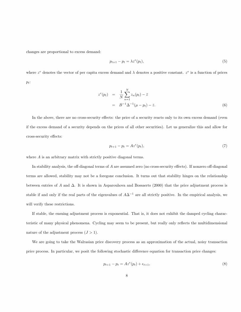
changes are proportional to excess demand:

pt+1 − pt = λze(pt), (5)

where ze denotes the vector of per capita excess demand and λ denotes a positive constant. ze is a function of prices

pt:

ze(pt) =1N

N∑n=1

zn(pt) − z̄

= B−1∆−1(µ − pt) − z̄. (6)

In the above, there are no cross-security effects: the price of a security reacts only to its own excess demand (even

if the excess demand of a security depends on the prices of all other securities). Let us generalize this and allow for

cross-security effects:

pt+1 − pt = Aze(pt), (7)

where A is an arbitrary matrix with strictly positive diagonal terms.

In stability analysis, the off-diagonal terms of A are assumed zero (no cross-security effects). If nonzero off-diagonal

terms are allowed, stability may not be a foregone conclusion. It turns out that stability hinges on the relationship

between entries of A and ∆. It is shown in Asparouhova and Bossaerts (2000) that the price adjustment process is

stable if and only if the real parts of the eigenvalues of A∆−1 are all strictly positive. In the empirical analysis, we

will verify these restrictions.

If stable, the ensuing adjustment process is exponential. That is, it does not exhibit the damped cycling charac-

teristic of many physical phenomena. Cycling may seem to be present, but really only reflects the multidimensional

nature of the adjustment process (J > 1).

We are going to take the Walrasian price discovery process as an approximation of the actual, noisy transaction

price process. In particular, we posit the following stochastic difference equation for transaction price changes:

pt+1 − pt = Aze(pt) + εt+1, (8)

8

where the noise εt+1 is assumed to be mean zero and uncorrelated with past information. Past information includes

everything that is available to all investors (order flow, transaction volume and prices). Let It denote this publicly

available information. In addition, we assume that the noise εt+1 is uncorrelated with the time-t excess demand as well.

Note that investors in general will not know the excess demand (because they may not know the aggregate per-capita

supply z̄ or because they may not know other investors’ risk aversion). That is, ze(pt) is not in It. Altogether, we

impose that:

E[εt+1|It] = 0, (9)

E[εt+1ze(pt)|It] = 0. (10)

2.3 Conjectures

The Walrasian model is used to formulate a number of conjectures, to be verified empirically later on. The conjectures

not only address the relationship between excess demands and transaction price changes, but include a few hypotheses

about how excess demands are expressed in the market place and, hence, about the channels through which excess

demands influence price changes.

A. [Role Of Excess Demand] A security’s transaction price changes and its excess demand (as defined in general

equilibrium theory) are positively correlated.

B. [Cross-Security Effects] A security’s transaction price changes and the excess demands of other securities are

not correlated. (This is the standard assumption in stability analysis; there is no specific justification for it other

than that it would be hard to imagine theoretically why cross-security effects exist.)

C. [Stability] The Walrasian system of stochastic difference equations – see (8) – mean-reverts to the equilibrium

price configuration.

9

D. [Link Between Excess Demand And The Book] There is correlation between information in the book and

excess demands.

E. [The Quality Of A Market] Changes in the book correlate with transaction price changes that are not

explained by excess demands.

The last two conjectures concern the link between excess demands and price changes. It is hypothesized that

excess demands are to a certain extent expressed in the book, so that excess demands affect transaction prices partly

through the book. This contrasts with some recent game-theoretic models of the dynamics of an open book system

(the trading mechanism used in the experiments), where fundamental information is deliberately chosen to influence

prices only through transactions, because traders with information that affects the fundamental value of an asset are

not allowed to make a market or submit limit orders.5

We will explore the validity of these conjectures on an extensive dataset of order and transaction activity from a

number of large-scale experiments ran with Caltech’s Marketscape trading interface. Let us discuss the data first.

3 Description of data

To evaluate the predictive power of our equilibration models, we collected transaction price changes in a series of

large-scale financial markets experiments run through Caltech’s internet-based Marketscape trading system over the

last two years. While prices in these experiments generally moved in the direction predicted by asset pricing theory,

most transactions clearly occurred before markets reached equilibrium. Experimental data allow us to determine when

markets are not in equilibrium. In field studies, such a clean delineation is impossible, absent precise knowledge of

the economic structure of the market (parameters of demand and supply). In fact, it has been tradition in empirical

finance to just treat all observations as if they are snapshots of a dynamic equilibrium, ignoring the very premise5See footnote 2 for an elaboration on this point.

10

underlying this article, namely, that markets may at times be in disequilibrium. Moreover, the experimental setup

allows us to estimate excess demand with little error. Estimation of excess demand in field data is far more difficult,

absent knowledge of investors’ beliefs, a good model for attitudes towards risk, and the total supply of assets.

The three-asset experiments are described in more detail in Bossaerts and Plott (1999) (focusing on pricing),

Bossaerts, Plott and Zame (2001) (focusing on allocations) and Bossaerts, Plott and Zame (2002) (formally linking

prices and allocations). The Appendix to previous drafts of this article6 also discusses evidence from a number of

four-asset experiments. We will briefly refer to those later on. The basic setup for all experiments was the same. A

web-based, continuous open book trading system was used, called Marketscape.7 In the three-asset experiments, two

assets, A and B, were risky. The third one, the “Note”, was riskfree. In addition, subjects were given a limited amound

of cash. Payoffs (dividends) on the risky securities depend on a state variable. Three states were possible and one

was drawn at random, with a commonly known distribution. The number of subjects ran from less than 20 to over 60.

In each of several consecutive periods the assets were allocated, mostly unevenly, across subjects. The markets were

then opened for a fixed period of time. When the period closed the state was announced and earnings recorded. New

allocations of the asset were distributed and a fresh period opened. Subjects whose earnings were sufficiently low

were declared bankrupt and were prevented from participating in subsequent periods. Earnings ranged from nothing

(the bankrupt) to over two hundred dollars.

In the three-security experiments, the payoff matrix remained the same, namely:6A draft with a discussion of the four-asset experiments can be retrieved at ftp://ftp.hss.caltech.edu/pub/pbs/pdiscempir01 02.pdf.7Instructions and screens for the experiment we discuss here can be viewed at http://eeps3.caltech.edu/market-001005 and use identi-

fication number:1 and password:a to login as a viewer. The reader will not have a payoff but will be able to see the forms used. If the

reader wishes to interact with the software in a different context, visit http://eeps.caltech.edu and go to the experiment and then demo

links. This exercise will provide the reader with some understanding of how the software works.

11

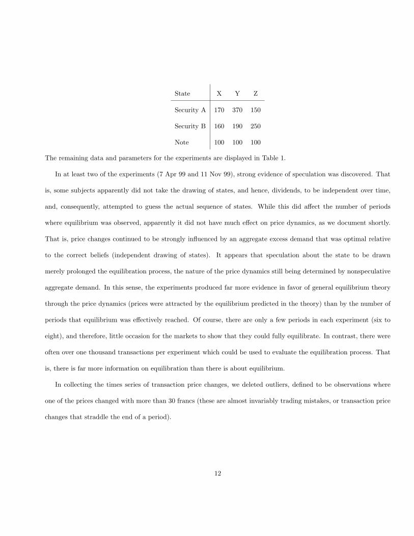
State X Y Z

Security A 170 370 150

Security B 160 190 250

Note 100 100 100

The remaining data and parameters for the experiments are displayed in Table 1.

In at least two of the experiments (7 Apr 99 and 11 Nov 99), strong evidence of speculation was discovered. That

is, some subjects apparently did not take the drawing of states, and hence, dividends, to be independent over time,

and, consequently, attempted to guess the actual sequence of states. While this did affect the number of periods

where equilibrium was observed, apparently it did not have much effect on price dynamics, as we document shortly.

That is, price changes continued to be strongly influenced by an aggregate excess demand that was optimal relative

to the correct beliefs (independent drawing of states). It appears that speculation about the state to be drawn

merely prolonged the equilibration process, the nature of the price dynamics still being determined by nonspeculative

aggregate demand. In this sense, the experiments produced far more evidence in favor of general equilibrium theory

through the price dynamics (prices were attracted by the equilibrium predicted in the theory) than by the number of

periods that equilibrium was effectively reached. Of course, there are only a few periods in each experiment (six to

eight), and therefore, little occasion for the markets to show that they could fully equilibrate. In contrast, there were

often over one thousand transactions per experiment which could be used to evaluate the equilibration process. That

is, there is far more information on equilibration than there is about equilibrium.

In collecting the times series of transaction price changes, we deleted outliers, defined to be observations where

one of the prices changed with more than 30 francs (these are almost invariably trading mistakes, or transaction price

changes that straddle the end of a period).

12

4 Estimation Strategy

The purpose of the empirical exercise is to shed light on the conjectures in Section 2.3, primarily by estimating the

system of stochastic difference equations in (8). The main stumbling block in estimation of these equations is the

determination of the excess demands.

Excess demand is a quantity (measured as number of assets) that is at the core of general equilibrium theory. It

equals the theoretical optimal aggregate demand at last prices, minus the aggregate supply. Per capita aggregate supply

varied substantially across experiments, but remained fairly constant within an experiment.8 Our using experimental

data is fortunate here, because aggregate supply is a design element in the experiments, and hence, known to the

experimenter (but only to the experimenter - subjects were not given any information about supplies). In the field,

aggregate supply is virtually impossible to measure.9

In contrast, per-capita aggregate demand is more difficult to obtain. It depends on subjects’ risk attitudes. It is

well known that individual risk attitudes can hardly be identified as the mean-variance preferences behind the CAPM.

Still, Bossaerts, Plott and Zame (2001) documents that mean-variance optimality characterizes aggregate demand.

The drawback is that aggregate demand could be obtained only up to an unknown constant, the harmonic mean risk

aversion (B in (6)). We decided to arbitrarily set B equal to 10−3. The arbitrariness of this choice has no qualitative

effect on the estimation results, because the error in B is absorbed in an intercept that we chose to add to the basic

equation (8).

To see this, use (6) (the definition of excess demand) and (8) (the Walrasian stochastic difference equations) to

derive the following. Let B̂ denote one’s estimate of B (in our case, B̂ = 10−3). Appeal to the fact that per-capita

8Within the reported experiments, aggregate supply changed only as a result of subjects being excluded from trading because they ran

a negative balance two periods in a row.9This fact led to the Roll critique of tests of the CAPM. See Roll (1977).

13

aggregate supply z̄ hardly varies during an experiment, so that we can take it to be constant.

pt+1 − pt

= Aze(pt) + εt+1

= A

(1B

∆−1(µ − pt) − z̄

)+ εt+1

= (B̂

B− 1)Az̄ +

B̂

BA

(1B̂

∆−1(µ − pt) − z̄

)+ εt+1. (11)

Inspection of these equations reveals that the following are the effects of errors in the estimation of harmonic mean

risk aversion B.

• The intercept is nonzero unless B̂ = B.

• The diagonal elements of the slope coefficient matrix remain positive if they were originally.

• The off-diagonal elements of the slope coefficient matrix remain nonzero if they originally were, and do not

change signs.

• The properties of the error term are unaffected.

Consequently, the fact that we cannot measure exactly the harmonic mean risk aversion B has little impact on our

inference. In particular, we can still determine the signs of the elements of A, which is crucial in evaluating the merit

of the conjectures in Section 2.3. We must allow for an intercept in the equations, however, to capture mis-estimation

of B.

One should contrast this with the difficulties encountered when using field data. To compute the theoretical excess

demand from field data, one would not only have to estimate B, but also the market’s assessments of the covariance

matrix ∆ and the vector of mean payoffs µ. In addition, while supplies of individual securities are known, it is

crucial that all relevant risky securities be incorporated into the analysis, but it is unclear what these are. The payoff

distribution and the supplies are known in an experimental setting, because they are part of the design. Finally, it is

14

doubtful that mean-variance optimality would provide an accurate description of aggregate demand in the field, for a

variety of reasons (most assets are long-lived; risk is much bigger; payoff distributions cannot simply be characterized

in terms of means and variances; payoff distributions vary over time in predictable ways; etc.).

5 Empirical Results

Let us discuss the evidence on each of the conjectures of Section 2.3 in turn.

A. Role Of Excess Demand

Estimation results for the basic system of difference equations (8) (allowing for an intercept, to capture mis-estimation

of the harmonic mean risk aversion) are reported in Table 2. Price changes are computed over transaction time: the

clock advances whenever one of the assets trades; the price changes for the assets that do not trade are set equal to

zero. (We will consider an alternative time measurement below, to check robustness of the results.)

Confirming our conjecture, excess demand and subsequent transaction price changes are strongly positively cor-

related. The F -statistics are high and the p-levels are uniformly below 1%. The relationship is very noisy, however,

because the R2s are generally low. That is, a large part of changes in transaction prices is uncorrelated with excess

demands. To a certain extent, this is caused by the high number of zero price changes induced by our measurement of

time (time advances whenever one of the securities trade, and we set the price change of the nontrading assets equal

to zero). We document below that the R2s rise when time is measured in terms of a security’s own transactions alone.

The low R2s are also to be attributed to variations in the book that are unrelated to changes in excess demand, as we

show later on.

To verify that the system of stochastic difference equations is well specified, so that statistical inference (standard

errors, F -tests) is reliable, Table 2 also reports autocorrelations of the error terms. The autocorrelation coefficients

are generally small, and significant at the 5% level in only two cases. The chance of finding at least two rejections at

15

the 5% level is about 1 in 9.

B. Cross-Security Effects

In contrast with the basic Walrasian model used in stability analysis, there is strong evidence of cross-security effects:

most often, there is a significant relationship between a security’s excess demand and another security’s subsequent

price change. See Table 2.

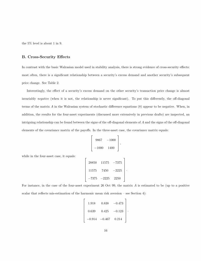
Interestingly, the effect of a security’s excess demand on the other security’s transaction price change is almost

invariably negative (when it is not, the relationship is never significant). To put this differently, the off-diagonal

terms of the matrix A in the Walrasian system of stochastic difference equations (8) appear to be negative. When, in

addition, the results for the four-asset experiments (discussed more extensively in previous drafts) are inspected, an

intriguing relationship can be found between the signs of the off-diagonal elements of A and the signs of the off-diagonal

elements of the covariance matrix of the payoffs. In the three-asset case, the covariance matrix equals: 9867 −1000

−1000 1400

,

while in the four-asset case, it equals: 28850 11575 −7375

11575 7450 −2225

−7375 −2225 2250

.

For instance, in the case of the four-asset experiment 26 Oct 99, the matrix A is estimated to be (up to a positive

scalar that reflects mis-estimation of the harmonic mean risk aversion – see Section 4):1.918 0.838 −0.473

0.639 0.425 −0.123

−0.914 −0.467 0.214

.

16

The pattern of signs of the entries of the estimate of A matches that of the signs of the entries of the covariance matrix

of payoffs.

The finding is unlikely to be coincidence. Its implications shed new light on the issue of stability. From (6), the

inverse covariance matrix can be recognized to be proportional to the Jacobian (matrix of first derivatives) of the

excess demands. More specifically, letting J denote this Jacobian,

J = −B−1∆−1.

We find that the adjustment matric A is related to the covariance matrix ∆, and hence, to the Jacobian of the excess

demands J . The above example indicates that the relationship is almost proportional: A = γ∆ = −γBJ−1, for some

positive scalar γ. That is, the market’s price discovery process is:

pt+1 − pt = −γBJ−1ze(pt) + εt+1. (12)

Ignoring the stochastic term, this is the set of difference equations that represents the Newton procedure for the

numerical solution of the set of equations

ze(pt) = 0.

But the latter defines equilibrium! Consequently, it appears that markets use the Newton procedure in their search

for equilibrium. Because the Newton procedure is stable,10 markets will eventually always discover the equilibrium

prices. We leave it to future work to explore explanations for the relationship between price discovery and Newton’s

procedure.11

A+B. Robustness Check

So far, we have been measuring price changes under a clock that advances whenever one of the securities trades. The

transaction price changes of the nontrading securities are set equal to zero. Because of this, many transaction price10Except where the Jacobian equals zero, which it never is in this case.11For an analysis of the Newton procedure in the context of computation of general equilibrium, see Judd (1998).

17

changes are zero and the inference may have been affected accordingly.

To check robustness of the inference to variations in time measurement, Table 3 replicates the previous table

whereby price changes are now recorded under each security’s own transaction time clock. For security A, for instance,

time advances only when it trades and not when security B or the Note trades.

There is no qualitative effect on the inference. As expected, the R2s increase. The conclusions about the role of

excess demand and the cross-security effects are upheld. In many cases, however, the error term becomes significantly

negatively autocorrelated, presumably as a result of bid-ask bounce. The negative autocorrelation makes inference

less reliable (standard errors are mis-specified; they are likely to be under-estimated) than under the alternative time

measurement.

C. Stability

The finding of significant cross-security effects raises the possibility that the Walrasian system is unstable, which

means that prices may cycle around the equilibrium or even diverge. If indeed there is a relationship between the

adjustment matrix (A) and the Jacobian of excess demands, then stability will obtain, as mentioned before.

Here, we explore stability directly. For the system of stochastic difference equations to be stable, the real parts of

the eigenvalues of the adjustment matrix (A) times the inverse covariance matrix of payoffs (∆−1) must all be strictly

positive. Because of potential mis-estimation of the harmonic mean risk aversion, the matrix of slope coefficients in

the projection of transaction price changes onto excess demands estimates A only up to a scalar. See (11). Since this

scalar will be strictly positive, however, the requirement on the real parts of the eigenvalues of A∆−1 is fulfilled if the

same holds for the eigenvalues of the matrix of slope coefficients times ∆−1.

Table 4 reports the results of tests of these stability conditions. Stability obtains in all experiments. Somehow,

markets manage to generate dynamics that guarantee mean-reversion back to the general equilibrium. Future research

should be aimed at investigating how. Potential answers will emerge once an explanation for the cross-security effects

18

is found.

D. Link Between Excess Demands And The Book

We conjectured that excess demands are expressed in part through the book. The book is, of course, very complex.

We need a convenient summary of the information in the book, with the risk of finding no relationship with excess

demands if our summary measure is not appropriate.

Practitioners often suggest that the relative thickness of the two sides of the book provides useful information to

gauge the direction of the markets if change is to take place. For instance, if there are far more bid quotes that are

tightly packed together whereas ask quotes are fewer and far apart, then transaction price changes are more likely to

increase even if market buy and sell orders of the same size are submitted with the same probability. This suggests

the following statistic.

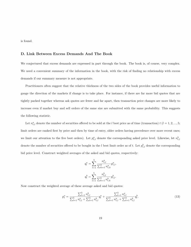
Let nat,l denote the number of securities offered to be sold at the l best price as of time (transaction) t (l = 1, 2, ..., 5;

limit orders are ranked first by price and then by time of entry, older orders having precedence over more recent ones;

we limit our attention to the five best orders). Let pat,l denote the corresponding asked price level. Likewise, let nb

t,l

denote the number of securities offered to be bought in the l best limit order as of t. Let pbt,l denote the corresponding

bid price level. Construct weighted averages of the asked and bid quotes, respectively:

qat =

5∑l=1

nat,l∑5

k=1 nat,k

pat,l,

qbt =

5∑l=1

nbt,l∑5

k=1 nbt,k

pbt,l.

Now construct the weighted average of these average asked and bid quotes:

pot =

∑5l=1 nb

t,l∑5l=1 na

t,l +∑5

l=1 nbt,l

qat +

∑5l=1 na

t,l∑5l=1 na

t,l +∑5

l=1 nbt,l

qbt . (13)

19

Our predictor of the transaction price change equals po minus the last transaction price change, i.e., pot − pt.12 We

will refer to our predictor as the signal in the book or the weighted average quote.

Instead of projecting pot − pt onto excess demands, we project it onto the difference between the last transaction

price and the price at which our estimate of excess demand equals zero (i.e., our estimate of the equilibrium price).

The two projections are equivalent, of course, because the excess demands are but a linear transformation of the

difference between the last transaction price and the equilibrium price:

ze(pt) =1B

∆−1(µ − pt) − z̄

=1B

∆−1(p∗t + B∆z̄ − pt) − z̄

=1B

∆−1(p∗t − pt).

We will refer to p∗t − pt as the excess demands signal. Projection of the signal in the book onto the excess demands

signal rather than onto excess demands themselves facilitates interpretation of the slope coefficients, as will become

clear soon.

Table 5 demonstrates that the signal in the book is correlated with the excess demands signal. The projections are

almost uniformly significant, and the R2s are sometimes remarkably high (up to 18%). When the slope coefficients

on a security’s own excess demand signal are significant, their sign is uniformly negative. This is intuitive: it implies

that the more the transaction price is below the equilibrium price, the higher the price signal in the book. We posited

that relative thinness of the book at one side predicts that transaction prices are more likely to move in the direction

of thinness, and hence, in the direction of our “signal in the book.” The empirical results then imply that the book

predicts price increases when transaction prices are below equilibrium prices.

Our finding that the book is correlated with excess demand suggests that access to the book is valuable, which12When one side of the book is empty, po

t is not defined. In that case, we set pot − pt equal to its time series average. To avoid outliers

when one side of the book is very thin and the bid-ask spread is very wide, we set pot −pt equal to its time series average whenever it would

otherwise be bigger than 50 francs (which corresponds roughly to 25% of the expected payoff).

20

explains the reluctance of some traders in field markets to expose the book to the public at large.

E. The Quality Of A Market

Table 6 documents that the signal in the book (our weighted average of the quotes) generally correlates with the error

of the Walrasian model. That is, the book explains in part transaction price changes that are uncorrelated with excess

demand. The support is not uniform, but it should be pointed out that the dependent variable is but an estimate (of

the error of the Walrasian model), and hence, the projections may not be very powerful.

It is clear that the quality of a market (i.e., its ability to discover general equilibrium) can be enhanced if the book

better reflects excess demand. This raises the issue of how to incentivize traders to expose their willingness to trade

in the form of limit orders in the book. We leave design of such incentive schemes for future work.

6 Conclusion

We study price dynamics from more than 11,000 transactions in several large-scale financial market experiments. First,

we test two simple principles of equilibration, namely, that (i) a security’s price changes are positively correlated with

its own excess demand, and (ii) there are no cross-security effects (the price changes of a security are not influenced

by excess demand for other securities). These principles form the core of the Walrasian price discovery model usually

assumed in general equilibrium stability analysis.

The data strongly supported the first principle. However, we found systematic cross-security effects whose pres-

ence potentially invalidates many stability results. Still, despite this theoretical possibility, stability obtained in all

experiments. What emerges is a curious pattern in the cross-security effects: their sign correlates almost perfectly

with the sign of the corresponding payoff covariance.

To a certain extent, the finding that excess demand and transaction price changes are correlated should come as

a surprise, because our markets were not organized as a Walrasian tatonnement. Moreover, orders in the book are

21

usually for fairly small quantities, well below excess demands.

Next, we investigate how excess demands translate into transaction price changes. In particular, we posit that

the book plays a crucial role, in contrast with the passive role of liquidity provider assumed in many microstructure

models. Confirming our conjecture, we observe strong correlation between excess demand and the “shape” of the book

(measured as weighted averages of the quotes).

The correlation between excess demand and the book was far from perfect, which might explain why it often

takes relatively long before markets equilibrate, and why markets can still move away even after reaching equilibrium.

Indeed, we find that the book explained part of the variance of transaction price changes that is unaccounted for by

excess demand.

Our findings raise new questions that we plan to explore in the future. Foremost, we need to better understand

the cross-security effects and the curious correlation between them and the corresponding payoff covariances. They

may provide an explanation for the stability of the price discovery processes in the experiments, as they suggest a link

between price discovery in real markets and the Newton procedure in numerical computation of general equilibrium.

Second, price discovery will be enhanced if the book were to better reflect excess demand. Incentive mechanisms need

to be explored that increase the correlation between the book and excess demand.

22

References

Anderson, C.M., S. Granat, C. Plott and K. Shimomura, 2000, Global Instability in Experimental General Equilibrium:

The Scarf Example, Caltech working paper.

Arrow, K. and F. Hahn, 1971, General Competitive Analysis (Holden-Day, San Francisco).

Asparouhova, E. and P. Bossaerts, 2000, Competitive Analysis Of Price Discovery In Financial Markets, Caltech

working paper.

Bossaerts, P. and C. Plott, 1999, Basic Principles of Asset Pricing Theory: Evidence from Large-Scale Experimental

Financial Markets, Caltech working paper.

Bossaerts, P., C. Plott and W. Zame, 2001, Prices And Allocations In Financial Markets: Theory and Evidence,

Caltech working paper.

Bossaerts, P., C. Plott and W. Zame, 2001, Structural Econometric Tests Of General Equilibrium Theory On Data

From Large-Scale Experimental Financial Markets, Caltech working paper.

Glosten, L., 1994, Is the Electronic Limit Order Book Inevitable? Journal of Finance 49, 1127-1161.

Glosten, L. and P. Milgrom, 1985, Bid, Ask, and Transaction Prices in a Specialist Market with Heterogeneously

Informed Traders, Journal of Financial Economics 14, 71-100.

Judd, K., 1998, Numerical Methods in Economics (MIT Press, Cambridge, MA).

Kyle, A.P., 1985, Continuous Auctions and Insider Trading, Econometrica 53, 1315-35.

Negishi, T., 1962, The Stability Of The Competitive Equilibrium. A Survey Article, Econometrica 30, 635-70.

Roll, R., 1977, A Critique Of The Asset Pricing Theory’s Tests, Part I: On The Past And Potential Testability Of

The Theory, Journal Of Financial Economics 4, 129-76.

23

Sand̊as, P., 2001, Adverse Selection and Competitive Market Making: Empirical Evidence from a Limit Order Market,

Review of Financial Studies 14, 705-734.

Seppi, D., 1997, Liquidity Provision with Limit Orders and a Strategic Specialist, Review of Financial Studies 10,

103-150.

Scarf, H., 1960, Some Examples of Global Instability of the Competitive Equilibrium, International Economic Review

1, 157-172.

24

Table 1: Experimental design data.

Experiment Subject Signup Endowments Cash Loan Exchange

Category Reward A B Notes Repayment Rate

(Number) (franc) (franc) (franc) $/franc

7 Oct 98 30 0 4 4 0 400 1900 0.03

16 Nov 98 23 0 5 4 0 400 2000 0.03

21 0 2 7 0 400 2000 0.03

11 Feb 99 8 0 5 4 0 400 2000 0.03

11 0 2 7 0 400 2000 0.03

7 Apr 99 22 175 9 1 0 400 2500 0.03

22 175 1 9 0 400 2400 0.04

10 Nov 99 33 175 5 4 0 400 2200 0.04

30 175 2 8 0 400 2310 0.04

11 Nov 99 22 175 5 4 0 400 2200 0.04

23 175 2 8 0 400 2310 0.04

04 Aug 00 8 0 5 4 0 400 2200 0.04

7 0 2 8 0 400 2310 0.04

05 Oct 00 8 0 5 4 0 400 2200 0.04

7 0 2 8 0 400 2310 0.04

25

Table 2: Estimation Of The Walrasian Stochastic Difference Equations

Experiment Security Coefficientsa R2 F -statisticb Nc ρd

Intercept Excess Demande

A B

7 Oct 98 A 1.568 0.800 -0.152 0.04 13.6 614 -0.03

(0.340) (0.153) (0.057) (< .01)

B -0.602 -0.096 0.187 0.08 25.1 614 0.05

(0.168) (0.076) (0.028) (< .01)

16 Nov 98 A 0.451 0.581 -0.057 0.03 14.1 1053 −0.10∗∗

(0.121) (0.110) (0.014) (< .01)

B -0.126 -0.063 0.023 0.01 3.5 1053 0.00

(0.092) (0.084) (0.011) (.03)

11 Feb 99 A 0.666 0.671 -0.044 0.03 7.8 466 -0.03

(0.413) (0.181) (0.038) (< .01)

B -0.934 -0.297 0.093 0.03 6.5 466 0.05

(0.278) (0.122) (0.026) (< .01)

7 Apr 99 A 1.097 0.561 -0.043 0.03 19.8 1385 -0.03

(0.189) (0.090) (0.011) (< .01)

B 0.371 0.130 0.011 0.01 6.5 1385 −0.06∗

(0.135) (0.064) (0.008) (< .01)

10 Nov 99 A 0.568 0.993 -0.085 0.05 34.9 1318 -0.04

(0.136) (0.121) (0.013) (< .01)

B -0.045 0.240 -0.006 0.01 8.8 1318 -0.04

(0.110) (0.098) (0.011) (< .01)

11 Nov 99 A 0.843 0.505 0.000 0.03 18.1 1190 -0.04

(0.164) (0.087) (0.014) (< .01)

B -0.047 0.039 0.058 0.02 14.0 1190 -0.05

(0.135) (0.072) (0.012) (< .01)

04 Aug 00 A 1.701 0.689 -0.126 0.03 5.3 312 -0.11

(0.525) (0.219) (0.045) (< .01)

B -0.514 0.034 0.182 0.08 13.1 312 -0.03

(0.560) (0.234) (0.048) (< .01)

05 Oct 00 A 0.584 0.835 -0.102 0.04 8.6 194 0.03

(0.760) (0.305) (0.056) (< .01)

B -1.592 -0.438 0.126 0.03 6.2 194 -0.10

(0.740) (0.297) (0.055) (< .01)

aOLS projections of transaction price changes onto (i) an intercept, (ii) the estimated excess demands for the two risky securities

(A and B). See (8). Time advances whenever one of the three assets trades. Standard errors in parentheses.bp-level in parentheses.cNumber of observations.dAutocorrelation of the error term; ∗ and ∗∗ indicate significance at the 5% and 1% level, respectively.eEstimated on the basis of harmonic mean risk aversion equal to 10−3. Error in estimation of the harmonic mean risk aversion

will be absorbed in the intercept.

26

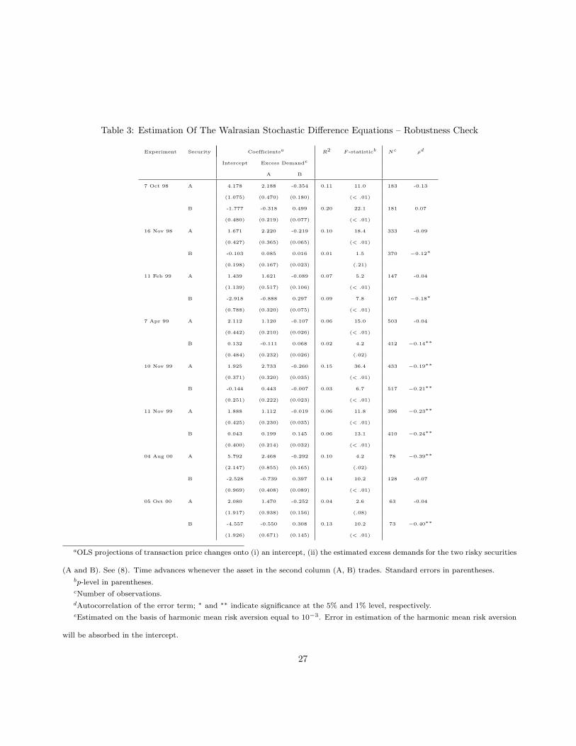
Table 3: Estimation Of The Walrasian Stochastic Difference Equations – Robustness Check

Experiment Security Coefficientsa R2 F -statisticb Nc ρd

Intercept Excess Demande

A B

7 Oct 98 A 4.178 2.188 -0.354 0.11 11.0 183 -0.13

(1.075) (0.470) (0.180) (< .01)

B -1.777 -0.318 0.499 0.20 22.1 181 0.07

(0.480) (0.219) (0.077) (< .01)

16 Nov 98 A 1.671 2.220 -0.219 0.10 18.4 333 -0.09

(0.427) (0.365) (0.065) (< .01)

B -0.103 0.085 0.016 0.01 1.5 370 −0.12∗

(0.198) (0.167) (0.023) (.21)

11 Feb 99 A 1.439 1.621 -0.089 0.07 5.2 147 -0.04

(1.139) (0.517) (0.106) (< .01)

B -2.918 -0.888 0.297 0.09 7.8 167 −0.18∗

(0.788) (0.320) (0.075) (< .01)

7 Apr 99 A 2.112 1.120 -0.107 0.06 15.0 503 -0.04

(0.442) (0.210) (0.026) (< .01)

B 0.132 -0.111 0.068 0.02 4.2 412 −0.14∗∗

(0.484) (0.232) (0.026) (.02)

10 Nov 99 A 1.925 2.733 -0.260 0.15 36.4 433 −0.19∗∗

(0.371) (0.320) (0.035) (< .01)

B -0.144 0.443 -0.007 0.03 6.7 517 −0.21∗∗

(0.251) (0.222) (0.023) (< .01)

11 Nov 99 A 1.888 1.112 -0.019 0.06 11.8 396 −0.23∗∗

(0.425) (0.230) (0.035) (< .01)

B 0.043 0.199 0.145 0.06 13.1 410 −0.24∗∗

(0.400) (0.214) (0.032) (< .01)

04 Aug 00 A 5.792 2.468 -0.292 0.10 4.2 78 −0.39∗∗

(2.147) (0.855) (0.165) (.02)

B -2.528 -0.739 0.397 0.14 10.2 128 -0.07

(0.969) (0.408) (0.089) (< .01)

05 Oct 00 A 2.080 1.470 -0.252 0.04 2.6 63 -0.04

(1.917) (0.938) (0.156) (.08)

B -4.557 -0.550 0.308 0.13 10.2 73 −0.40∗∗

(1.926) (0.671) (0.145) (< .01)

aOLS projections of transaction price changes onto (i) an intercept, (ii) the estimated excess demands for the two risky securities

(A and B). See (8). Time advances whenever the asset in the second column (A, B) trades. Standard errors in parentheses.bp-level in parentheses.cNumber of observations.dAutocorrelation of the error term; ∗ and ∗∗ indicate significance at the 5% and 1% level, respectively.eEstimated on the basis of harmonic mean risk aversion equal to 10−3. Error in estimation of the harmonic mean risk aversion

will be absorbed in the intercept.

27

Table 4: The Walrasian Model: Stability

Experiment Eigenvalues Of A∆−1 (∗10−4)a

First Second

7 Oct 98 1.33 0.80

16 Nov 98 0.59 0.13

11 Feb 99 0.59 + 0.19i 0.59 − 0.19i

7 Apr 99 0.61 0.15

10 Nov 99 1.05 0.11

11 Nov 99 0.70 0.32

04 Aug 00 1.31 0.77

05 Oct 00 0.98 0.48

aFor stability, the real parts of the eigenvalues of A∆−1 should all be strictly positive.

28

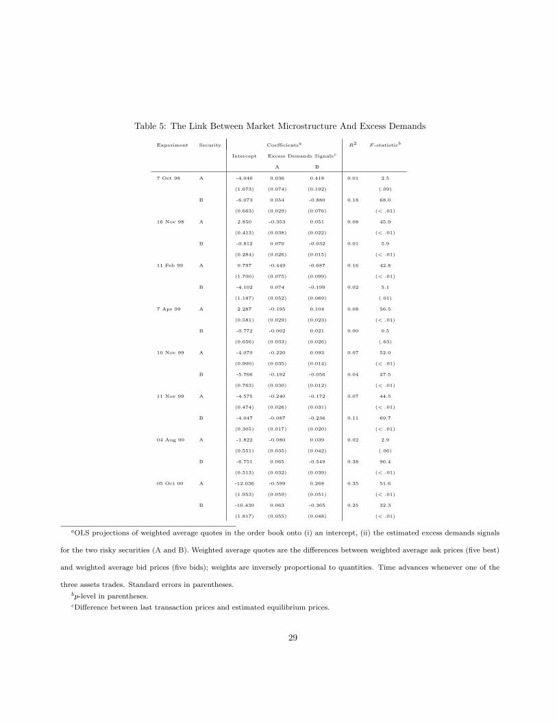
Table 5: The Link Between Market Microstructure And Excess Demands

Experiment Security Coefficientsa R2 F -statisticb

Intercept Excess Demands Signalsc

A B

7 Oct 98 A -4.046 0.036 0.418 0.01 2.5

(1.673) (0.074) (0.192) (.09)

B -6.073 0.054 -0.880 0.18 68.0

(0.663) (0.029) (0.076) (< .01)

16 Nov 98 A 2.850 -0.353 0.051 0.08 45.9

(0.413) (0.038) (0.022) (< .01)

B -0.812 0.070 -0.032 0.01 5.9

(0.284) (0.026) (0.015) (< .01)

11 Feb 99 A 0.797 -0.449 -0.687 0.16 42.8

(1.700) (0.075) (0.099) (< .01)

B -4.102 0.074 -0.199 0.02 5.1

(1.187) (0.052) (0.069) (.01)

7 Apr 99 A 2.287 -0.195 0.104 0.08 56.5

(0.581) (0.029) (0.023) (< .01)

B -0.772 -0.002 0.021 0.00 0.5

(0.656) (0.033) (0.026) (.63)

10 Nov 99 A -4.070 -0.220 0.093 0.07 52.0

(0.900) (0.035) (0.014) (< .01)

B -5.766 -0.192 -0.056 0.04 27.5

(0.763) (0.030) (0.012) (< .01)

11 Nov 99 A -4.575 -0.240 -0.172 0.07 44.5

(0.474) (0.026) (0.031) (< .01)

B -4.047 -0.087 -0.236 0.11 69.7

(0.305) (0.017) (0.020) (< .01)

04 Aug 00 A -1.822 -0.080 0.039 0.02 2.9

(0.551) (0.035) (0.042) (.06)

B -6.751 0.065 -0.549 0.38 96.4

(0.513) (0.032) (0.039) (< .01)

05 Oct 00 A -12.036 -0.599 0.268 0.35 51.6

(1.953) (0.059) (0.051) (< .01)

B -10.430 0.063 -0.365 0.25 32.3

(1.817) (0.055) (0.048) (< .01)

aOLS projections of weighted average quotes in the order book onto (i) an intercept, (ii) the estimated excess demands signals

for the two risky securities (A and B). Weighted average quotes are the differences between weighted average ask prices (five best)

and weighted average bid prices (five bids); weights are inversely proportional to quantities. Time advances whenever one of the

three assets trades. Standard errors in parentheses.bp-level in parentheses.cDifference between last transaction prices and estimated equilibrium prices.

29

Table 6: Quality Of The Market

Experiment Security Coefficientsa R2 F -statisticb

Intercept Weighted Average Quotec

A B

7 Oct 98 A 0.065 0.012 -0.003 0.00 1.1

(0.092) (0.008) (0.019) (.33)

B 0.025 0.004 -0.000 0.00 0.6

(0.046) (0.004) (0.009) (.46)

16 Nov 98 A 0.003 0.006 0.020 0.00 1.4

(0.064) (0.009) (0.013) (.26)

B 0.005 0.009 0.035 0.01 7.2

(0.049) (0.007) (0.010) (< .01)

11 Feb 99 A -0.004 0.001 0.007 0.00 0.2

(0.129) (0.011) (0.017) (0.92)

B 0.036 -0.003 0.049 0.05 11.3

(0.085) (0.007) (0.011) (< .01)

7 Apr 99 A 0.026 0.030 -0.000 0.01 6.6

(0.035) (0.008) (0.008) (< .01)

B 0.021 0.003 0.025 0.02 10.7

(0.025) (0.006) (0.006) (< .01)

10 Nov 99 A 0.042 0.028 -0.019 0.01 5.7

(0.054) (0.009) (0.011) (< .01)

B -0.017 -0.013 0.025 0.01 5.0

(0.044) (0.007) (0.009) (.01)

11 Nov 99 A 0.008 0.044 -0.021 0.02 10.1

(0.050) (0.010) (0.015) (< .01)

B 0.060 -0.017 0.070 0.03 16.7

(0.041) (0.008) (0.013) (< .01)

04 Aug 00 A 0.270 0.152 0.022 0.06 9.6

(0.141) (0.035) (0.029) (< .01)

B 0.144 0.028 0.071 0.02 2.6

(0.154) (0.038) (0.032) (.08)

05 Oct 00 A 0.015 0.004 0.009 0.00 0.0

(0.373) (0.029) (0.034) (.95)

B 0.111 0.033 0.066 0.03 2.8

(0.358) (0.028) (0.032) (.06)

aOLS projections of the error of the Walrasian price discovery model (8) (see Table 2) onto (i) an intercept, (ii) the weighted

average quotes in the order book for the two risky securities (A and B). Time advances whenever one of the three assets trades.

Standard errors in parentheses.bp-level in parentheses.cDifference between weighted average ask prices (five best) and weighted average bid prices (five bids); weights are inversely

proportional to quantities.

30