exchange rate volatility and the two margins of trade
TRANSCRIPT

Exchange Rate Volatility and the two Margins
of Trade: Evidence from Monthly Trade Data
Authors: Florian JohannsenA
Inmaculada Martinéz-ZarzosoB,A
Filiations: A Georg-August Universität Göttingen, Germany B Universitat Jaume I, Spain
JEL classification: F15, F36
Contact Information
Address: Florian JohannsenChair of Economic Theory and Development EconomicsPlatz der Göttinger Sieben 337073 GöttingenGermany
Email: [email protected]

Table of Contents
I - Introduction 1
II - Literature 2 II.I - Theory 2II.II - Empirical Findings 6II.III - The Euro Effect 10II.IV - Summary 14
III - Empirics 14 III.I - Equation 16III.II - Data 17III.III - Exclusion Restriction 18III.IV - Measuring Volatility 19
IV - Results 20 IV.I - Exchange Rate Volatility and Trade 25IV.II - Exchange Rate Movements 26IV.III - The European Union 27IV.IV - The Euro 27
V - Conclusion 27 V.I - Policy Implications 28
VI - Bibliography I
VII - Appendix VII
Index of Tables
Table 1: Variables 15Table 2: Control Variables 16Table 3: Coverage 17Table 4: BEC Categories 18Table 5: Regression Results - Capital Goods 22Table 6: Regression Results - Intermediates 23Table 7: Regression Results - Final Goods 24Table 8: Beta Coefficients of the Volatility Measure 26Table 9: Correlation between Volatility Measure and its Lags 26Table 10: Impact of Euro in Percentage Change 27Table 11: Fixed Effects Regressions - Capital Goods IXTable 12: Fixed Effects Regressions - Intermediates IXTable 13: Fixed Effects Regressions - Final Goods X

I - Introduction
The end of the Breton Woods system in the early 1970's and the adoption of a floating exchange
rate regime in 1973 raised the question of how the resulting increase in exchange rate volatility
causes exchange rate risk and affects international trade and welfare. The EMU and the
introduction of the Euro, associated with the abolition of several European currencies, lead to a
huge debate among economists about the effects on trade.
Very recently, the global fnancial crisis as well as the catalyst of the debt crises and the massive
central bank interventions, especially in Europe and the U.S. have increased exchange rate
volatility again and brought the topic back on the agenda.
In the light of the recent events, especially the case of Europe and the Euro is worth a second
glance. The question whether joining a currency union and thereby eliminating exchange rate
volatility with various other countries is boosting trade signifcantly is a very relevant question for
many Central and Eastern European countries. Countries like Poland postponing their accession to
the Euro are a strong indicator for that.
As theoretical predictions concerning the impact of uncertainty induced by exchange rate volatility
on trade have ambiguous results, empirical investigations are expedient to validate or to reject the
various existing theories.
The aim of this paper is to provide further evidence on the relationship between exchange rate
volatility, common currencies and trade by presenting several novelties with respect to previous
research. Higher frequency trade data is used to take into account the short term effects of
volatility. Disaggregated trade data is used to deal with differences among industries, especially
between agricultural and manufactures and intermediates and fnal products. In contrast to many
other studies, several econometric problems including the existence of zero trade values are taken
into account. Investigating the impact of exchange rate volatility and the Euro at the same time
allows to disentangle the effect of a common currency beyond the elimination of any variation in
the exchange rate with other members.
1
Furthermore, due to a large dataset including very recent data, the developments of the past
years with the fnancial crisis and the EU enlargement to the east is covered, yielding additional
fndings and policy implications.
Our results show a positive effect on trade for a EU membership and negative impact of exchange
rate volatility, but ambiguous results for a Euro membership and. We also found different effects
for the intensive and extensive margin of trade.
II - Literature
This chapter briefly introduces theoretical predictions and fndings and the applied econometric
approaches to investigate the relationship between exchange rate volatility and trade. This issue
has been examined very intensively, thus a broad range of theoretical and empirical literature
exists and several survey papers provide a good overview (Côté 1994; McKenzie 1999; Ozturk
2006; Bahmani-Oskooee & Hegerty 2007; Auboin & Ruta 2011).
Furthermore, the literature on the very related but distinct Euro-effect with the paper of Rose
(2000) being the initial is brought into a common context.
II.I - Theory
As mentioned before, theoretical studies have shown mixed effects. Most describe negative
effects for an increase of exchange rate volatility on trade due to rising levels of uncertainty. Clark
(1973) describes the case of a single frm with no market power producing under perfectly
competitive conditions a single good without imported components that is entirely exported to
one foreign market. The frm gets paid in the foreign currency and has to convert the proceeds at
the current exchange rate. As movements of the exchange rate are unpredictable and access to
currency hedging is assumed to be limited, the proceeds vary. High costs for adjustments to the
scale of production keep the frm from altering output in advance of the realization of the
exchange rate. Thus, uncertainty about future exchange rates directly translates into uncertainty
about future receipts in domestic currency.
Under the assumption that the frm is risk averse and maximizes profts, the frm has to determine
a level of output that incorporates this uncertainty. In this situation, the variability of profts
depends completely on changes in the exchange rate. Thus, an increase in volatility of the
2

exchange rate – while the average level remains unchanged – leads to a decrease in production,
and hence in exports, due to the increased exchange rate risk. This very simple theoretic model
was later refned by Hooper & Kohlhagen (1978), yielding the same clear negative result for
exchange rate volatility and trade.
However, these theoretical fndings are based on rather strong assumptions, notably no hedging
opportunities either through the forward exchange market or through offsetting transactions, no
imported inputs, risk aversion of the exporter, no ability to pile up stocks, no adjustments to the
scale of production and perfect competition are assumed.
Importing intermediates from the export destination partly offsets negative effects in case the
foreign currency depreciates, as prices for the inputs decline as well. Multinational frms are
engaged in trade and fnancial transactions of different nature across various countries with
independently floating exchange rates. This allows them to exploit movements in the exchange
rates by holding a portfolio of assets and liabilities in different currencies (Makin 1978).
Furthermore, exchange rates have the tendency to adjust quickly to changes in inflation rates.
Lower revenues due to a depreciating foreign currency are then at least partly offset by the higher
nominal export price (Cushman 1983; Cushman 1986).
When the assumption that frms cannot alter the scale of production and adjust at least some of
the factors of production is relaxed, frms can even proft in terms of higher average revenues
from higher volatility by increasing production when the currency depreciates (Canzoneri & Clark
1984). The effect depends on the ability of the frm to adjust inputs and switch export markets and
the degree of risk aversion. The risk for the exporter consists of to components: There is the
currency risk that frms can diversify by mixing local and foreign currency invoicing and there is a
price risk as the quantity demanded is uncertain because the price facing the buyer is itself
uncertain. The higher variability of expected profts in times of stronger volatility will lead to lower
production when risk aversion is high. If risk aversion is relatively low, the positive effect of greater
price variability on expected profts outweighs the negative impact of the higher variability of
profts, and the frm will raise the average capital stock and the level of output and exports.
Unambiguous positive effects were confrmed by Broll & Eckwert (1999), at least for frms that are
flexible and can reallocate their products among markets in the short term according to changes in
3

the exchange rates. At the same time, the frms need strong domestic demand for their products
they can rely on. The authors see the home market as the save harbour and exporting as an option
for additional revenues with the domestic price for their products being the “strike” price. Still, as
higher volatility leads to higher risks, the effect in the end depends on the degree of risk aversion.
Nevertheless, volatility is increasing the value of a frm's options to export by increasing the
potential gains from trade.
Paradoxically, very risk averse frms could export more when exchange rate volatility rises to
compensate expected falls in revenues. This is described for the case, that the income effect of
reduced utility derived from higher uncertainty of revenues overcompensates the substitution
effect of higher exchange rate risk (De Grauwe 1988). Furthermore, positive effects depend on the
aggregate exposure to risk (Viaene & de Vries 1992) and the type of shocks frms are exposed to
(Barkoulas et al. 2002).
Financial hedging via exchange markets can reduce uncertainty generated by fluctuations the
nominal exchange rates. Unfortunately, it is not available for all frms to due to different stages of
development of the fnancial markets (Baron 1976). Furthermore, contracts are typically cover
rather large amounts, maturities are short and costly. Coverage is usually very restricted, only a
limited share of possible fluctuations is covered and only during the proposed maturities. These
characteristics make hedging more available for bigger exporting frms as they are less likely to
face liquidity constraints (Baldwin & Krugman 1989). Obstfeld & Rogoff (1998) fnd that risk-
adverse frm use hedging instruments and that utilizing those instruments leads to higher export
prices. This results in lower (world) output and consumption.
Another aspect is the role of “sunk costs” in international trade relations that came up with the
hysteresis literature and beter fts modern trade paterns (Krugman 1986; Franke 1991; Dixit
1989). The concept is that a large share of international trade consists of differentiated
manufactured goods that typically require signifcant investment by frms to set up marketing and
distribution networks, to adapt their products to foreign markets, and to set up production
facilities specifcally designed for export markets. Hence, fxed costs are large and if spent once,
frms will stay in the foreign market when revenues fall, as long as they can recover the variable
costs. Firms are less reactive and tend to a “wait-and-see” attitude and wait for the exchange rate
to turn around to recoup the entry costs or “sunk costs”. For the frms however, larger fluctuations
4
are an incentive to stay out of foreign markets they are not active in yet and to stay in markets
they have already invested in. Thus, for frms more volatile exchange rates can be seen as an
encouragement towards inertia.
To take into account complex interactions of the variables in the models, the relationship between
exchange rate volatility on trade was examined in a general equilibrium framework. This allows, in
contrast to the partial equilibrium framework, all variables that may have an impact on the level of
trade to change. Baccheta & van Wincoop (2000) employed a two-country, general equilibrium
model where uncertainty arises from monetary, fscal, and technology shocks, and compared the
level of trade and welfare for fxed and floating exchange rate arrangements. In their model trade
is determined by the certainty equivalent of a frm’s revenue and costs in the domestic market
relative to the foreign market, whereas the welfare of the country is determined by the volatility
of consumption and leisure. Their main conclusion is, that no clear relationship between the level
of trade and the type of exchange rate arrangement exist, as the result depends on consumer
preferences with regard to consumption and leisure and the rules for monetary policy followed.
Therefore, if a monetary stimulus in a country leads to the depreciation of the currency, the effect
on trade might be litle. Certainly, the depreciation reduces imports, but due to monetary stimulus
domestic demand may boost imports and offset the effect. The net effect depends on various
factors like demand elasticities for imports, price stickiness and the ability of the supply side to
match demand.
As Baccheta & van Wincoop (2000) point out, the level of trade does not provide a good index of
the level of welfare in a country, and thus there is no one-to-one relationship between levels of
trade and welfare in comparing exchange rate systems. Obstfeld & Rogoff (1998) fnd that the
elimination of exchange rate volatility could result in a welfare gain of up to one percent of GDP by
extending the new open economy macroeconomic model to an explicitly stochastic environment
where price-setting decisions of frms are affected by risk. The model was extended by Bergin &
Tchakarov (2003) to allow for incomplete asset markets and investment by frms. They fnd that
the welfare costs are generally quite small, on the order of one tenth of one percent of
consumption but can under certain certain conditions reach the order of the results of Obstfeld &
Rogoff (1998). Therefore, consumers need to exhibit considerable persistence in their patern of
consumption, such that welfare is adversely affected by sudden changes in consumption, and
5

asset markets are asymmetric in the way that there is only one international bond, thus that the
country without its own bond is adversely affected. Barkoulas et al. (2002) state that in open
economies fluctuations of trade flows can signifcantly impact the variability of the overall level of
economic activity resulting in fnancial sector illiquidity, reductions in real output or heightened
inflationary pressures.
More recently, (Broll et al. 2006) study the optimum production decision of an international frm
employing the mean-standard deviation model. They fnd that an increase in the exchange rate
risk has an unambiguous impact on trade. The result depends on the elasticity of risk aversion with
respect to the standard deviation of the frm’s random proft.
Taking into account the heterogeneity of frms in the light of the “new-new” trade models,
Berman et al. (2009) analyse differences in the reaction of frms to changes in the exchange rate.
In their model, frms differ in terms of performance which is measured by a mix of productivity and
quality benchmarks. It is assumed that only the best performing frms in terms of low fxed costs
export, but exchange rate depreciation is an incentive to enter export markets. Their fndings
suggest that while high productivity frms optimally raise their markup rather than the volume of
exports, low productivity frms choose the opposite strategy and thus, pricing to market is both
endogenous and heterogenous. Due to the fxed costs to export only high productivity frms can
export, hence those frms which precisely react to an exchange rate depreciation by increasing
their export price rather than their sales. This leads to a very limited impact of exchange rate
movements on aggregate trade volumes because of the “natural” selection process. They test the
main predictions of the model on a French frm level data set with destination-specifc export
values and volumes on the period from 1995 to 2005 and the results confrm the theoretical
predictions.
II.II - Empirical Findings
The empirical fndings reflect the above mentioned ambiguous theoretical results.
Investigating the results of the empirical literature for the years 1978 to 2003, Coric & Pugh (2010)
fnd that the empirical literature on exchange rate variability and trade reveals a modestly
negative relationship with pronounced heterogeneity.
6
Recent studies are more likely to yield signifcant results. Klein & Shambaugh (2006) fnd
signifcant positive effects examining exchange rate volatility within the gravity framework and
controlling for exchange rate regimes with a sample of 181 countries and the period of 1973-1999.
For the period of 1980-2005 Ozturk & Kalyoncu (2009) fnd signifcant negative effects for Republic
of Korea, Pakistan, Poland and South Africa, but a positive effect for Turkey and Hungary in the
long using an Engle-Granger residual-based cointegrating technique. Rahman & Serletis (2009) fnd
that exchange rate uncertainty has a generally negative and signifcant effect on U.S. exports, but
that exports responded asymmetrically to positive and negative exchange rate shocks.
In a gravity model using quarterly instead of yearly data, Chit et al. (2010) examined the impact of
exchange rate volatility on exports among fve East Asian countries and their exports to thirteen
industrialized countries. They fnd statistically negative effects for absolute volatility for their
sample of countries. Additionally, they provide evidence that the relative volatility is important as
well by testing for the impact of the volatility between third countries.
Eicher & Henn (2011) investigate the impact of currency unions and employ the gravity equation
for a huge panel of countries. They include exchange rate volatility as a control variable which has
no robust effects, while they fnd a signifcant positive effect for currency unions.
For the very specifc case of Norway with several changes in monetary policy regime, Boug &
Fagereng (2010) fnd no effect for exchange rate volatility on export performance using
cointegrated Vector Autoregression framework.
Baum & Caglayan (2010) examine the case of numerous industrial countries for the period 1980-
1998, but cannot determine a signifcant effect for exchange rate uncertainty on bilateral trade
flows. However, the impact of exchange rate volatility on the volatility of bilateral trade flows is
signifcant and positive. Using quarterly data from 1977-2003, Hondroyiannis et al. (2008)
investigate the relationship between exchange rate volatility and aggregate export volumes for 12
developed economies in a model that includes real export earnings of oil-producing economies as
a determinant of industrial-country export volumes. The fnd no evidence for a signifcant impact
at any time of their sample.
In order to deal with the aggregation bias, that results from estimating the gravity equation with
aggregate data when the trade costs and elasticities vary at a sectoral level, Anderson & van
7

Wincoop 2004, suggest that employing the gravity equation at a sectoral level can improve the
reliability of the results. Furthermore, since the currency and timeframe of contracting, the
openness to international trade, the degree of homogeneity or the storability of goods vary over
sectors, it is important to take industry related differences into account and to control for them.
Empirical studies fnd robust evidence for a downward bias (e.g. Anderson & Yotov 2010), thus
there is evidence that usage of data that is disaggregated at an appropriate level is preferable.
Investigating the impact of the exchange rate on trade relations between China and the U.S. from
1978-2002 for 88 sectors, Bahmani-Oskooee & Y. Wang (2007) show that sectors react very
differently to changes in the real exchange rate and that thus employing disaggregated trade data
yields beter results trade paterns. To examine the impact of the volatility of the exchange rate,
trade relations between the U.S. and Japan for 117 industries for the period from 1973 to 2006
was studied by Bahmani-Oskooee & Hegerty (2008) in a similar fashion. What they fnd is that
some industries are influenced by exchange rate volatility in the short-run, although this effect is
ofen ambiguous. In the long-run, trade shares of most industries are relatively unaffected by
exchange rate uncertainty, while some industries experience a relative shif in their proportion of
overall trade. A study on sectoral bilateral trade with Malaysia by Bahmani-Oskooee & Hanafah
(2011) yields similar results. Confrming the importance of sectoral differences, K.-L. Wang &
Barret (2007) fnd that exchange rate volatility only has a signifcant impact on agricultural
exports from Taiwan to the U.S., leaving all other sectors unaffected. Cho et al. (2002) also fnd
negative long term effects for agricultural products with a panel of ten OECD countries and the
period from 1974 to 1995.
Byrne et al. (2008) fnd a negative impact on US im- and exports from and to several European
countries. The effect is strongest and only robust for differentiated goods what they atribute to
bigger importance of knowledge for the these type of goods. As gaining the necessary knowledge
about a certain market is expensive, switching markets is more difficult when the needed amount
of knowledge per market is higher.
For trade flows of China, the Euro area and the United States in two sectors, namely agriculture
and manufacturing and mining, Huchet-Bourdon & Korinek (2011) fnd that that exchange
volatility impacts trade flows only slightly with litle differences between the two sectors.
However, they state that these results may change when small or developing countries are
8

examined. Changes in the level of the exchange rate affect both sectors signifcantly, but do not
completely explain the trade imbalances in the three countries examined.
Another important aspect is how the relationship between exchange rate volatility and trade is
affected by the stage of development of the countries investigated. Caglayan & Di (2010)
investigate monthly sectoral bilateral US trade flows with the thirteen biggest trading partners.
They fnd evidence that developing countries are more likely to be affected than developed
countries but they fnd no evidence for differences between sectors. As Grier & Smallwood (2007)
point out, results for developing countries could be more likely to be signifcant as a well
developed fnancial market is necessary to provide frms with adequate hedging instruments at a
reasonable price. In a study investigating the impact on nine developed and nine developing
countries they fnd that real exchange rate volatility is more likely to have a signifcant negative
impact on international trade for developing countries, than on advanced economies. Contrary to
that, Wei (1999) fnds no empirical evidence for the hypothesis that the availability of hedging
instruments reduces the impact of exchange rate volatility on trade.
In a very broad study covering 39 countries, several volatility measures and different econometric
specifcations, Clark et al. (2004) investigate the impact of exchange rate volatility on trade flows.
Their fndings are mixed and depend heavily on the empirical specifcation. In most cases the
authors fnd a negative relationship for short-run and long-run volatility, but when allowing for
time-varying country fxed effects, results turn insignifcant. While they fnd the choice of the
volatility measure not to have a signifcant impact on the result, the sample choice of countries
has it. Exchange rate volatility appears to have bigger impact on developing than advanced
economies. They conclude that in case "exchange rate volatility has a negative effect on trade, this
effect would appear to be fairly small and is by no means a robust".
To provide an overview of the empirical literature, Coric & Pugh (2010) conduct a meta-regression
analysis (MRA) for 58 studies. They fnd the relationship between exchange rate volatility and
trade to have modestly negative relationship with pronounced heterogeneity and litle evidence of
publication bias together with mainly positive evidence that this relationship is an authentic
empirical effect. Their results show that uncertainty arising from exchange rate volatility should be
a serious concern for least developed countries. This suggests that the availability of hedging
instruments is important.
9
Another potential bias emerges from a volatility measure constructed with low frequency
exchange rate data. This “temporal aggregation” of quarterly or monthly exchange rates tends to
reduce the variability of the exchange rates (K.-L. Wang et al. 2002) and thus hinder identifying the
true relationship between exchange rate uncertainty and trade. Since trade contracts in many
industries include an agreement on delivery within 90 days, even quarterly data may bias results
and make it impossible to identify short-term fluctuations in bilateral trade volumes as a
consequence of changes in the volatility of the bilateral exchange rate (Auboin & Ruta 2011).
In general, studies employing the gravity equation in international trade models are more likely to
fnd a negative relationship between exchange rate volatility and trade (Coric & Pugh 2010).
However, Clark et al. (2004) argue that most of these fndings are not robust to a more general
specifcation of the gravity equation that embodies the recent theoretical advances. As awareness
about potential biases within the gravity framework rises, more recent results tend to be
ambiguous (Eicher & Henn 2011). Disaggregated trade data is more likely to yield robust results,
but not for all countries and all sectors. Sample choice may also affect results as countries tend to
react differently to exchange rate shocks (Baum et al. 2004) and the effect might have changed
over time.
II.III - The Euro Effect
In January 1999, eleven European countries entered into currency union, that can be seen as one
of the most ambitious political and economic projects in the past decades. While common
currency arrangements in general are rather prevalent, the Euro is unique in terms of the number
of countries, their economic power and the fact that no single country has an unambiguous
leading role.
The question is how does the introduction of the Euro affect trade relations of the member states
and whether or not there is an effect beyond the afore discussed elimination of the nominal
exchange rate volatility.
Baldwin et al. (2005) contribute a model that puts explanations about how the euro could have
promoted trade beyond the effect of eliminated exchange rate volatility on a theoretical basis. It
predicts a convex relationship between trade volumes and exchange rate uncertainty meaning
that a marginal increase in trade as volatility falls gets progressively larger as volatility approaches
10

zero. They explain the non-convexity of the trade-volatility link with the fact that small frms are
affected more than large frms. Reductions in exchange rate volatility lead to increasing sales per
exporting frm and a higher number of exporting frms, thus intensive and extensive margin of
trade are affected. The second stems from the fact that the distribution of frms is skewed heavily
towards small frms, especially in Europe. In their model, the effect of volatility on trade depends
on the marginal costs faced by exporting frms and they therefore suggest the use of
disaggregated trade data to reflect differences in the cost structure among industries.
The basic idea of a convex relationship between exchange rate volatility is portrayed in Figure 1. At
high levels of volatility in the nominal exchange rate, trade is affected only slightly and changes in
total trade are mainly driven by the intensive margin, big frms expanding their exports as volatility
goes down. As volatility approaches zero, a large number of small frms starts exporting what
boosts trade via the extensive margin (Mongelli & Vega 2006).
Furthermore, currency unions are expected to reduce trade costs between its members by
eliminating the need to engage resources in handling currency exchange and facilitating price
comparisons.
Figure 1: Convex Relationship between Volatility and Trade
11
Trad
e Vo
lum
e
Volatility
Linear Volatility Effect
Euro Trade Effect

The literature studying the effect of Euro on trade empirically can be divided in studies
investigating currency union effects in general and studies employing Eurozone data. While the
later suffer from the rather small time frame of the Euro existence, the biggest drawback of the
pre-Euro studies is that the number of currency unions in the history is rather small and that the
unions usually consist of only two countries.
The initial spark for the empirical pre-Euro literature was the paper by Rose (2000) who estimated
a gravity equation with bilateral trade data for 186 countries and includes controls for exchange
rate volatility. He fnds that countries that join into a currency union together trade about 3 times
more with each other than we would expect otherwise. This was the starting point for an intensive
discussion about the employed estimation methodology and the interpretation of the ensuing
results.
In a theoretical derivation of the gravity model, Baldwin (2006) points out that the previous
literature including the paper of Rose (2000) neglects to control simultaneously for general
equilibrium effects1 and unobserved bilateral heterogeneity among the trade partners. Beyond
technical problems, there are many other reasons why early studies can hardly deliver a good
estimate of theEuro effect on trade. Among others, the aforementioned small number currency
unions and the fact that most unions consist of large economy and one or more very small
economies. Furthermore, many currency unions in the world before the Euro can be described has
hub-and-spoke currency arrangements and consist of a former colonial power (e.g. USA, France,
Britain, Australia, New Zealand and Denmark) and several of its former colonies. The decision to
start or end a currency union or Dollarization usually must be seen in the context of political and
economic changes that drive the decision. These can be for example revolutions, external pressure
in the time of the cold war or struggles afer independence and are very likely to have a severe
impact on trade relations with the (former) partner country and thus to bias estimation results. As
a currency union between an african country with its former colonizer is in its nature different to a
currency union among similar western countries, results can hardly be transferred and it shows
how exceptional the case of the Eurozone is.
When testing their aforementioned theoretical model empirically with a gravity equation and
controls for exchange rate volatility and a Eurozone-membership both included, Baldwin et al.
1 ofen referred to as multilateral resistance
12

(2005) fnd the effect of exchange rate volatility on trade to be negative and the effect of the
common currency to be positive and large (still much smaller than the effect found by Rose
(2000) and both to be signifcant.
In a broad meta-regression analysis, Havránek (2010) fnds that when correcting for publication
bias results for a Euro effect are insignifcant, while other currency unions yield signifcant positive
effects of more than 60%.
In order to evaluate the importance of the problems in the econometric specifcation of the early
study by Rose (2000) that were raised by Baldwin (2006), Eicher & Henn (2011) implement
Baldwin’s econometric specifcation to provide an updated benchmark. They fnd that the proper
use of controls reduces omited variable bias and lowers the magnitudes but not the signifcance
of average currency union trade effects, effects vary to a great extent between different unions
and the effect to be smaller than the effect of preferential trade agreements.
One of the frst studies to estimate the Euro effect with a proper data for the eurozone was
conducted by Flam & Nordström (2007). They use highly disaggregated trade data for the period
1995-2005 and 20 countries within the gravity framework. According to their results the level of
trade within the eurozone in 2002-2005 was 26% higher than the average level in 1995-1998 and
trade between the eurozone and the ten outsiders has increased by about 12% in both directions.
They fnd the increase in the extensive margin to be greater than in the intensive margin of trade,
thus the trade increase is driven rather by higher number of goods traded and goods been traded
between more countries than by an increase in the volume of trade that already existed before
the introduction of the Euro. This of course, can be seen as evidence for convex trade effects as
portrayed in Figure 1.
In one of the more recent atempts to explain high effects on trade found in other studies, Berger
& Nitsch (2008) use a dataset for 22 industrial countries for the years 1948 to 2003. They argue
that once they control for the positive trend in trade integration, the Euro has no signifcant
impact on trade. Furthermore, that measurable policy changes in areas such as exchange rate
policy and institutional integration have influenced the positive trend signifcantly and were
probably driving the effects in early studies. To similar results with respect to trade effects come
Santos Silva & Tenreyro (2010) using a differences-in-differences specifcation to compare the
13
exports of the frst twelve Euro-countries to those of similar groups of trading partners. They do
not fnd statistically signifcant effects on trade between Eurozone members following the
introduction of the Euro.
II.IV - Summary
While studies investigating the relationship between exchange rate volatility and trade show a
very pronounced heterogeneity in the results, one can say that the empirical literature on Euro
effects has seen quite some evolution in a litle more than ten years. Starting with very high results
in early pre-Euro studies and lower and lower results as methods evolved. Studies employing Euro
data have found small or even insignifcant effects, but usually covered only the early members.
Studies employing early Eurozone data can assumed to be biased due to the boom in imports in
the periphery countries from other Eurozone members that, as we know today, was a
consumption and housing bubble that led to what is usually referred to as the European “debt
crises”. Trade effects for the early years, especially for fnal goods, can therefore be expected to be
overestimated. New Eurozone members with a different cultural and economic background may
face different effects on trade.
One has also to differentiate between studies that introduce exchange rate volatility and a dummy
for currency unions both into the same equation. When assuming a convex relationship between
trade and exchange rate volatility (Figure 1), studies are more likely to yield signifcant results for
exchange rate volatility when common currencies are controlled for to account for the convexity.
At the same time, the introduction of separate variables allows to disentangle the effect of
common currencies that goes beyond the elimination of exchange rates.
III - Empirics
The empirical analysis of our study is based on the standard gravity approach, where trade
between two countries is modelled as function of their “economic mass” and the distance
between them.
We estimate the effect of our exchange rate volatility measure and the dummies for mutual EU
and Euro membership on exports by following the literature that employs an extended version of
the standard gravity equation in international trade with time varying country-fxed effects. In
14
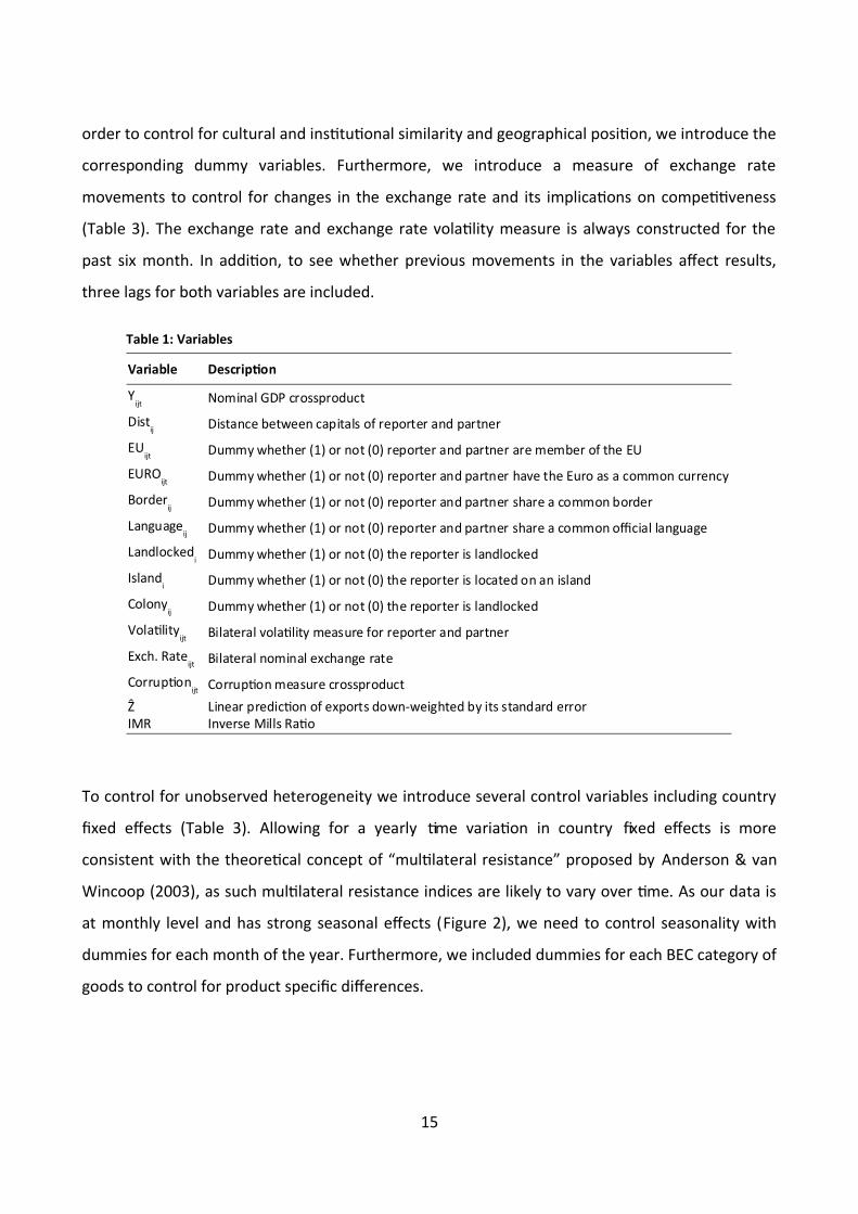
order to control for cultural and institutional similarity and geographical position, we introduce the
corresponding dummy variables. Furthermore, we introduce a measure of exchange rate
movements to control for changes in the exchange rate and its implications on competitiveness
(Table 3). The exchange rate and exchange rate volatility measure is always constructed for the
past six month. In addition, to see whether previous movements in the variables affect results,
three lags for both variables are included.
To control for unobserved heterogeneity we introduce several control variables including country
fxed effects (Table 3). Allowing for a yearly time variation in country fxed effects is more
consistent with the theoretical concept of “multilateral resistance” proposed by Anderson & van
Wincoop (2003), as such multilateral resistance indices are likely to vary over time. As our data is
at monthly level and has strong seasonal effects (Figure 2), we need to control seasonality with
dummies for each month of the year. Furthermore, we included dummies for each BEC category of
goods to control for product specifc differences.
15
Table 1: Variables
Variable Description
Nominal GDP crossproduct
Distance between capitals of reporter and partner
Dummy whether (1) or not (0) the reporter is landlocked
Dummy whether (1) or not (0) the reporter is located on an island
Dummy whether (1) or not (0) the reporter is landlocked
Bilateral volatility measure for reporter and partner
Bilateral nominal exchange rate
Corruption measure crossproductẐ Linear prediction of exports down-weighted by its standard error IMR Inverse Mills Ratio
Yijt
Distij
EUijt Dummy whether (1) or not (0) reporter and partner are member of the EU
EUROijt Dummy whether (1) or not (0) reporter and partner have the Euro as a common currency
Borderij Dummy whether (1) or not (0) reporter and partner share a common border
Languageij Dummy whether (1) or not (0) reporter and partner share a common official language
Landlockedi
Islandi
Colonyij
Volatilityijt
Exch. Rateijt
Corruptionijt

Estimations are conducted for three groups2: capital goods, intermediates and consumption
goods. The idea is that these three groups differ signifcantly in terms of contracting paterns and
that our variables of interest might affect differently or to a different extent trade flows.
III.I - Equation
First we are conducting year-varying country fxed-effects and random-effects regressions on the
log of the volume of bilateral exports. Therefor we are estimating the following equation:
ln X ijkt=β0+β1ln (Y it∗Y jt)+β2ln (Distanceij)+β3 EU ijt+β4 Euroijt+β5 Border ij+β6 Language ij+β7 Landlocked i+β8 Island i+β9Colony ij+
β10Volatilityijt+β11 ln (ExRate ijt)+β12Corruption ijt+αit+ν jt+εijkt, (1)
where the explained variable Xijt denotes nominal exports from the reporter to the partner
country. The simultaneous inclusion of the measure of nominal exchange rate volatility and the
dummy variable for mutual Euro membership allows us to capture convex effects (in case there
are any), although the volatility measure alone only captures linear effects.
A widely accepted treatment for the problems arising from zero trade flows os delivered by
Helpman et al. (2008) and also employed in this study: a two stage estimation including a Probit on
the likelihood that two countries trade (extensive margin), followed by a FGLS and a fxed-effects
estimation of the gravity equation to quantify the volume (intensive margin). The Inverse Mills
Ratio to control for sample selection bias and the linear prediction of exports down-weighted by
its standard error as proxy for frm heterogeneity are then included in the second stage regression.
The frst step estimation then is:
2 The groups were build following the classifcation of the United Nations Department of Economic and Social Affairs from 2007.
16
Table 2: Control Variables
Effect Control Dummies
Seasonality Dummy for each month of the yearProduct heterogeneity Dummy for each BEC product categoryTime and country specifc effects Dummy for each reporter/partner and year combination
Pijkt=β0+β1 ln (Y it∗Y jt)+β2 ln (Distanceij)+β3 EU ijt+β4 Euroijt+β5Border ij+β6 Language ij+β7 Landlocked i+β8 Island i+β9Colony ij+
β10Volatilityijt+β11 ln (ExRate ijt)+β12Corruption ijt+αit+ν jt+εijkt, (2)
followed by the second step:
ln X ijkt=β0+β1ln (Y it∗Y jt)+β2ln (Distanceij)+β3 EU ijt+β4 Euroijt+β5 Border ij+β6 Language ij+β7 Landlocked i+β8 Island i+β9Colony ij+β10Volatility ijt+β11ln (ExRateijt)+β12ZHAT+β13 IMR+αit+ν jt+ε ijkt
. (3)
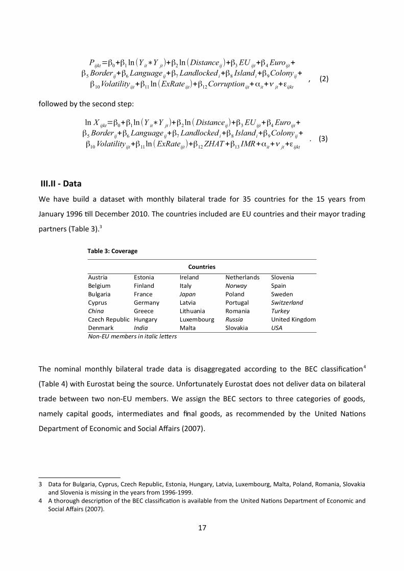
III.II - Data
We have build a dataset with monthly bilateral trade for 35 countries for the 15 years from
January 1996 till December 2010. The countries included are EU countries and their mayor trading
partners (Table 3).3
The nominal monthly bilateral trade data is disaggregated according to the BEC classifcation4
(Table 4) with Eurostat being the source. Unfortunately Eurostat does not deliver data on bilateral
trade between two non-EU members. We assign the BEC sectors to three categories of goods,
namely capital goods, intermediates and fnal goods, as recommended by the United Nations
Department of Economic and Social Affairs (2007).
3 Data for Bulgaria, Cyprus, Czech Republic, Estonia, Hungary, Latvia, Luxembourg, Malta, Poland, Romania, Slovakia and Slovenia is missing in the years from 1996-1999.
4 A thorough description of the BEC classifcation is available from the United Nations Department of Economic and Social Affairs (2007).
17
Table 3: Coverage
Countries
Austria Estonia Ireland Netherlands SloveniaBelgium Finland Italy Norway SpainBulgaria France Japan Poland SwedenCyprus Germany Latvia Portugal SwitzerlandChina Greece Lithuania Romania TurkeyCzech Republic Hungary Luxembourg Russia United KingdomDenmark India Malta Slovakia USANon-EU members in italic leters

Nominal GDP data is taken from the World Development Indicators database (WDI) at an annual
level. To construct the bilateral exchange rates5 and the volatility measure, we used Daily nominal
middle exchange rates by Datastream from the WM Company/Reuters.6
Variables identifying specifc geographical or cultural links are taken from the CEPII datasets.
III.III - Exclusion Restriction
To satisfy the exclusion restriction we need to exclude one variable from the second stage that has
no signifcant impact on the trade volume, but rather on the probability to export.
Most authors choose a dummy whether or not to countries share the same religion as the
excluded variable (Helpman et al. 2008). In the European context, we do not consider it a good
choice, as all countries share a christian heritage and only some of their trading partners differ
from that7.
5 The bilateral exchange rate measure is the average exchange rate of the past six months.6 This rate is the midpoint between the bid rate and the offered rate.7 Namely China, India and Turkey.
18
Table 4: BEC Categories
BEC Code Description
Food and beverages / primary / mainly for industryFood and beverages / primary / mainly for household consumptionFood and beverages / processed / mainly for industryFood and beverages / processed / mainly for household consumptionIndustrial supplies n.e.s. / primaryIndustrial supplies n.e.s. / processedFuels and lubricants / primary
321 Fuels and lubricants / processed / motor spiritFuels and lubricants / processed / otherCapital goods (except transport equipment)Capital goods / parts and accessories
510 Transport equipment and parts and accessories thereof / passenger motor carsTransport equipment and parts and accessories thereof / other / industrialTransport equipment and parts and accessories thereof / other / non-industrialTransport equipment and parts and accessories thereof / parts and accessor.Consumer goods n.e.s. / durableConsumer goods n.e.s. / semi-durableConsumer goods n.e.s. / non-durable
700 Goods not elsewhere specifed
1112
1123
1212
1223
2102
2202
3102
3222
4101
4202
5211
5223
5302
6103
6203
6303
Superscript denotes whether the category is 1 capital, 2 intermediate or 3 consumption good

In our eyes the crossproduct of the time varying measures of corruption for exporter and importer
is appropriate. The channel through which it takes effect is by rising insecurity and associated
extra fxed costs for the exporter in the form of authorities or criminals trying to extort bribes in
their homeland or export destination (Crozet et al. 2008).
For frms in countries with very low levels of corruption this can be seen as a serious obstacle to
start exporting as they are not used to this practices. But also positive effects for trade are
conceivable: corrupt officials might allow frms to export or import even if their products don't
meet technical, ethical, quality or safety standards. In overregulated countries this could lower
fxed trade costs signifcantly (Rose-Ackerman 1999).
Either way, by influencing fxed-costs rather than variable costs, corruption can be thought of as
an additional barrier to trade, that once frms have overcome it and know how to operate in a
corrupt environment, has no signifcant impact of the volume of trade.
The corruption data is taken from the International Country Risk Guide (ICRG) published by “The
PRS Group” and is a component of the Political Risk Dataset. It has a scale from 0 (extremely high
level of corruption) to 6 and assesses corruption within the political system8.
III.IV - Measuring Volatility
The measurement of exchange rate volatility can be conducted in many different ways. Most
approaches have in common to measure the variance, but differ in the implementation. Examples
are the standard deviation of a rate of change or the moving standard deviation. Other measures,
like ARCH and GARCH models, have gained popularity among researchers in recent years. The
later model the variance of the disturbance term for each period as a function of the errors in the
previous periods. All measures have drawbacks, like for instance the high persistence of real
exchange rate shocks when moving average representations are applied, or low correlation in
volatility when ARCH/GARCH models are the measure of choice (Baum et al. 2004). The
introduction of new and more sophisticated measures has however not changed the results in the
empirical literature on the impact of exchange rate volatility on trade signifcantly (Coric & Pugh
2010).
8 In our dataset the crossproduct ranges from 2 to 36.
19

Another important question is whether the volatility of the nominal or the real exchange rate is to
be used. While as an advantage the real exchange rate captures the true relative price of the good,
it also captures variation in the price levels, what is not desirable. Many studies use both exchange
rates and compare the results. The differences they fnd are usually very small.9
We are employing the standard deviation of the frst difference of logarithms, that has been used
in various studies before (e.g. Clark et al. (2004)). If the exchange rate is on a consistent trend,
which apparently could be forecasted and consequently would not be a source of uncertainty, the
measure has the ability that it will equal zero.
To avoid bias from changes in price levels via spurious correlation, we use nominal exchange rates.
The measure is constructed as a short-term volatility measure with bilateral exchange rates from
the past six month. Different to many other studies, we are constructing our exchange rate
volatility measure with daily exchange rates which allow more precise measures than end of the
month values, as exchange rates tend to more extreme movements at the end of each month.
High persistence of exchange rate shocks is less of a problem as we only measure very short-term
volatility of the past six months with high frequency data. In contrast to studies investigating long-
or mid-run volatility, we do not want to put weights on more recent volatility, as for a 6-month
volatility measure the, we expect movements in the exchange rate at each point of time to be
similarly important.
IV - Results
The estimation of the gravity equation yields the expected results for the standard variables.
Estimates are always signifcant and positive for the GDP crossproduct and negative and signifcant
for the distance between capitals. Controls for contiguity always yield signifcant positive
estimates and for one or both countries being islands estimates are negative and signifcant. While
the control variable for common official language yields mixed results, former colonial ties have
negative impact on the probability to export, but a positive on the volume.
The excluded variable in the second stage, that we expect to have an impact only on the
probability to trade, but not on the volume does a considerably good job. Our bilateral corruption
9 A very profound comparison of the effects real and nominal exchange rate volatility on exports was conducted by Coter & Bredin (2011) fnding that magnitude and direction are not changing, while timing effects can be different.
20

measure has an insignifcant impact on trade volume and a signifcant impact on the probability.
Only for capital goods, the impact on the volume is signifcant.
21
Table 5: Regression Results - Capital Goods
FE RE Probit FE RE0.447*** 0.474*** 0.462*** 0.243*** 0.467***(0.0395) (0.0128) (0.00222) (0.0402) (0.0127)
--1.206*** -0.861***
--1.206***
(0.0543) (0.00653) (0.0540)0.115*** 0.112*** 0.260*** 0.122*** 0.118***(0.0161) (0.0161) (0.0103) (0.0161) (0.0161)
-0.114*** -0.104*** -0.331*** -0.0708*** -0.0815***(0.0207) (0.0204) (0.0141) (0.0214) (0.0210)
-0.606*** 1.041***
-0.659***
(0.0976) (0.0337) (0.0984)
-0.194* 0.0408*
-0.207*
(0.112) (0.0243) (0.112)
-0.539*** -0.138***
-0.578***
(0.118) (0.0281) (0.118)
--0.698*** -0.247***
--0.723***
(0.195) (0.00772) (0.194)
--1.989*** -0.0988***
--2.004***
(0.251) (0.00744) (0.250)-2.805*** -2.758*** -1.688*** -1.518*** -2.231***
(0.514) (0.515) (0.368) (0.545) (0.542)-3.482*** -3.432*** -1.475*** -2.200*** -2.885***
(0.612) (0.614) (0.363) (0.638) (0.636)-3.527*** -3.425*** -1.430*** -2.244*** -2.901***
(0.509) (0.510) (0.358) (0.540) (0.537)-1.451*** -1.402*** -1.555*** -0.164 -0.735
(0.531) (0.533) (0.364) (0.559) (0.556)-0.301*** -0.296*** -0.00373 -0.299*** -0.295***(0.0710) (0.0712) (0.0501) (0.0709) (0.0712)0.0500 0.0578 -0.0924 0.0500 0.0571
(0.0634) (0.0636) (0.0840) (0.0634) (0.0636)0.271*** 0.240*** -0.0426 0.271*** 0.241***(0.0734) (0.0732) (0.0816) (0.0734) (0.0732)0.0826 0.0751 0.0656 0.0804 0.0733
(0.0547) (0.0549) (0.0471) (0.0547) (0.0548)-0.0089*** -0.0088*** 0.0156***
- -(0.00308) (0.00304) (0.000661)
Zhat - - -0.0088*** 0.0048***(0.00118) (0.00109)
IMR - - -2.047*** 5.926***(0.631) (0.509)
Obs. 283,895 283,895 345,268 283,895 283,8950.194 0.697 - 0.194 0.698
RMSE 1.171 1.176 - 1.171 1.175
1st Step 2nd Step 2nd Step
GDPijt
Distanceij
EUijt
Euroijt
Borderij
Languageij
Colonyij
Islandi
Landlockedi
Volatilityijt
L1.Volatilityijt
L2.Volatilityijt
L3.Volatilityijt
ExRateijt
L1.ExRateijt
L2.ExRateijt
L3.ExRateijt
Corruptionijt
R2
Standard errors in parentheses; signifcance levels: * 10% ** 5% ***1%

22
Table 6: Regression Results - Intermediates
FE RE Probit FE RE0.682*** 0.510*** 0.390*** 0.660*** 0.516***(0.0179) (0.0105) (0.000915) (0.0143) (0.0105)
--1.544*** -0.708***
--1.562***
(0.0489) (0.00278) (0.0488)0.0896*** 0.0873*** 0.341*** 0.0912*** 0.0890***(0.00902) (0.00901) (0.00449) (0.00900) (0.00900)0.0942*** 0.0894*** -0.257*** 0.0785*** 0.0705***(0.0116) (0.0115) (0.00613) (0.0120) (0.0119)
-1.147*** 1.096***
-1.107***
(0.0879) (0.0125) (0.0878)
-0.0904 0.117***
-0.0731
(0.102) (0.0102) (0.101)
-0.284*** -0.137***
-0.281***
(0.106) (0.0115) (0.106)
--0.570*** -0.193***
--0.582***
(0.170) (0.00348) (0.170)
--2.071*** -0.243***
--2.092***
(0.186) (0.00326) (0.186)-2.435*** -2.416*** -1.144*** -2.927*** -3.003***
(0.285) (0.285) (0.174) (0.299) (0.298)-2.560*** -2.522*** -0.868*** -3.033*** -3.090***
(0.339) (0.339) (0.171) (0.351) (0.350)-1.865*** -1.833*** -0.792*** -2.334*** -2.397***
(0.282) (0.282) (0.169) (0.296) (0.296)-0.617** -0.594** -2.426*** -1.086*** -1.153***(0.298) (0.298) (0.170) (0.312) (0.312)
-0.0911** -0.0904** 0.0503** -0.0911** -0.0904**(0.0394) (0.0394) (0.0230) (0.0394) (0.0394)0.0820** 0.0820** -0.0324 0.0824** 0.0824**(0.0349) (0.0349) (0.0385) (0.0348) (0.0349)-0.0136 -0.0145 -0.0392 -0.0134 -0.0142(0.0409) (0.0409) (0.0374) (0.0409) (0.0409)0.0191 0.0195 0.00306 0.0186 0.0188
(0.0301) (0.0301) (0.0216) (0.0301) (0.0301)0.00117 0.00180 -0.0020***
- -(0.00169) (0.00168) (0.000282)
Zhat - - --0.0013*** -0.0016***(0.000338) (0.000329)
IMR - - -2.545*** 2.833***(0.182) (0.178)
Obs. 1,045,992 1,045,992 1,381,072 1,045,992 1,045,9920.113 0.623 - 0.113 0.623
RMSE 1.243 1.244 - 1.243 1.244
1st Step 2nd Step 2nd Step
GDPijt
Distanceij
EUijt
Euroijt
Borderij
Languageij
Colonyij
Islandi
Landlockedi
Volatilityijt
L1.Volatilityijt
L2.Volatilityijt
L3.Volatilityijt
ExRateijt
L1.ExRateijt
L2.ExRateijt
L3.ExRateijt
Corruptionijt
R2
Standard errors in parentheses; signifcance levels: * 10% ** 5% ***1%
23
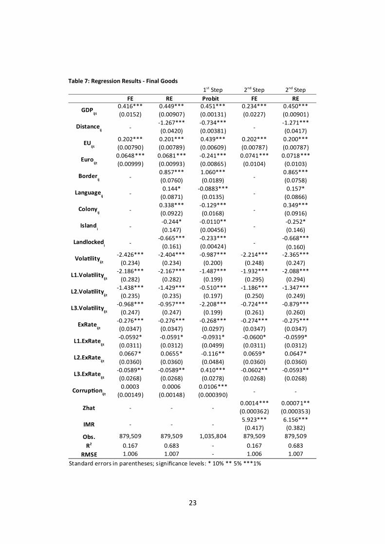
Table 7: Regression Results - Final Goods
FE RE Probit FE RE0.416*** 0.449*** 0.451*** 0.234*** 0.450***(0.0152) (0.00907) (0.00131) (0.0227) (0.00901)
--1.267*** -0.734***
--1.271***
(0.0420) (0.00381) (0.0417)0.202*** 0.201*** 0.439*** 0.202*** 0.200***(0.00790) (0.00789) (0.00609) (0.00787) (0.00787)0.0648*** 0.0681*** -0.241*** 0.0741*** 0.0718***(0.00999) (0.00993) (0.00865) (0.0104) (0.0103)
-0.857*** 1.060***
-0.865***
(0.0760) (0.0189) (0.0758)
-0.144* -0.0883***
-0.157*
(0.0871) (0.0135) (0.0866)
-0.338*** -0.129***
-0.349***
(0.0922) (0.0168) (0.0916)
--0.244* -0.0110**
--0.252*
(0.147) (0.00456) (0.146)
--0.665*** -0.233***
--0.668***
(0.161) (0.00424) (0.160)-2.426*** -2.404*** -0.987*** -2.214*** -2.365***
(0.234) (0.234) (0.200) (0.248) (0.247)-2.186*** -2.167*** -1.487*** -1.932*** -2.088***
(0.282) (0.282) (0.199) (0.295) (0.294)-1.438*** -1.429*** -0.510*** -1.186*** -1.347***
(0.235) (0.235) (0.197) (0.250) (0.249)-0.968*** -0.957*** -2.208*** -0.724*** -0.879***
(0.247) (0.247) (0.199) (0.261) (0.260)-0.276*** -0.276*** -0.268*** -0.274*** -0.275***(0.0347) (0.0347) (0.0297) (0.0347) (0.0347)-0.0592* -0.0591* -0.0931* -0.0600* -0.0599*(0.0311) (0.0312) (0.0499) (0.0311) (0.0312)0.0667* 0.0655* -0.116** 0.0659* 0.0647*(0.0360) (0.0360) (0.0484) (0.0360) (0.0360)
-0.0589** -0.0589** 0.410*** -0.0602** -0.0593**(0.0268) (0.0268) (0.0278) (0.0268) (0.0268)0.0003 0.0006 0.0106***
- -(0.00149) (0.00148) (0.000390)
Zhat - - -0.0014*** 0.00071**(0.000362) (0.000353)
IMR - - -5.923*** 6.156***(0.417) (0.382)
Obs. 879,509 879,509 1,035,804 879,509 879,5090.167 0.683 - 0.167 0.683
RMSE 1.006 1.007 - 1.006 1.007
1st Step 2nd Step 2nd Step
GDPijt
Distanceij
EUijt
Euroijt
Borderij
Languageij
Colonyij
Islandi
Landlockedi
Volatilityijt
L1.Volatilityijt
L2.Volatilityijt
L3.Volatilityijt
ExRateijt
L1.ExRateijt
L2.ExRateijt
L3.ExRateijt
Corruptionijt
R2
Standard errors in parentheses; signifcance levels: * 10% ** 5% ***1%

IV.I - Exchange Rate Volatility and Trade
Our six month measure for exchange rate volatility yields signifcant negative estimates for all
three categories of goods and also for all three lags.
Since comparing the impact of the volatility measure across goods and lags is difficult, we use the
beta coefficients of the regressions (Table 8). Beta coefficients are all measured in standard
deviations instead of the units of the variables. Thus, coefficients are all in the same standardized
units and one can compare these coefficients to assess the relative strength of each of the
predictors. A one standard deviation increase leads to a standard deviation increase in the
dependent variable in size of the beta coefficient, with the other variables held constant.
The beta coefficients indicate that the effect of exchange rate volatility is rather small, a one
standard deviation change in the volatility measure decreases trade volumes with between 0.0004
and 0.007 standard deviations.
The product categories seem to differ with respect to the timeframe of the effect on trade
volumes. While for fnal goods the frst measure has the biggest impact, it is the frst lagged
measure for intermediates and the second lagged measure for capital goods. Thus, fnal goods are
more affected from very recent volatility from the past six month and other goods more from
volatility longer ago.
The Heckman 2-stage approach changes results only slightly, yielding much lower estimates for
capital goods, a litle higher estimates for intermediates and slightly lower estimates for fnal
goods.
24

The volatility measure is modestly correlated with its lags. The correlation coefficients range
between 0.14 and 0.23 (Table 9).
IV.II - Exchange Rate Movements
Results for the measure for exchange rate movements for the past six months show a signifcant
negative impact, indicating that a depreciation of the foreign currency leads to lower export
volumes. The effect is stronger for capital and fnal goods, lying around 0.27 and 0.30, than for
intermediates lying around 0.09 all other variables held constant. Lags show mixed effects and
only in case of fnal goods all are signifcant at least at a 10% level.
When not controlling for exchange rate movements, coefficients for the dummies for EU and Euro
membership remain almost unchanged and coefficients for exchange rate volatility move slightly
(Table 11, Table 12 and Table 13).
25
Table 8: Beta Coefficients of the Volatility Measure
FE RE Probit FE REVolatility -0.00650 -0.00639 -1.60E-010 -0.00352 -0.00517
L1.Volatility -0.00837 -0.00825 -1.44E-010 -0.00529 -0.00694L2.Volatility -0.00857 -0.00832 -1.40E-010 -0.00545 -0.00705L3.Volatility -0.00361 -0.00348 -1.53E-010 -0.000408 -0.00183
Intermediates
Volatility -0.00500 -0.00497 -1.17E-010 -0.00601 -0.00617L1.Volatility -0.00548 -0.00540 -9.15E-011 -0.00649 -0.00661L2.Volatility -0.00404 -0.00397 -8.41E-011 -0.00506 -0.00519L3.Volatility -0.00134 -0.00129 -2.58E-010 -0.00235 -0.00250
Volatility -0.00612 -0.00607 -2.25E-010 -0.00559 -0.00597L1.Volatility -0.00565 -0.00560 -3.49E-010 -0.00499 -0.00539L2.Volatility -0.00380 -0.00377 -1.20E-010 -0.00313 -0.00356L3.Volatility -0.00258 -0.00255 -5.22E-010 -0.00193 -0.00234
1st Step 2nd Step 2nd Step
Capital Goods
Final Goods
Table 9: Correlation between Volatility Measure and its Lags
1.0000 0.2328 0.1637 0.1446
0.2328 1.0000 0.2268 0.1530
0.1637 0.2268 1.0000 0.2179
0.1446 0.1530 0.2179 1.0000
Volatilityijt
L1.Volatilityijt
L2.Volatilityijt
L3.Volatilityijt
Volatilityijt
L1.Volatilityijt
L2.Volatilityijt
L3.Volatilityijt
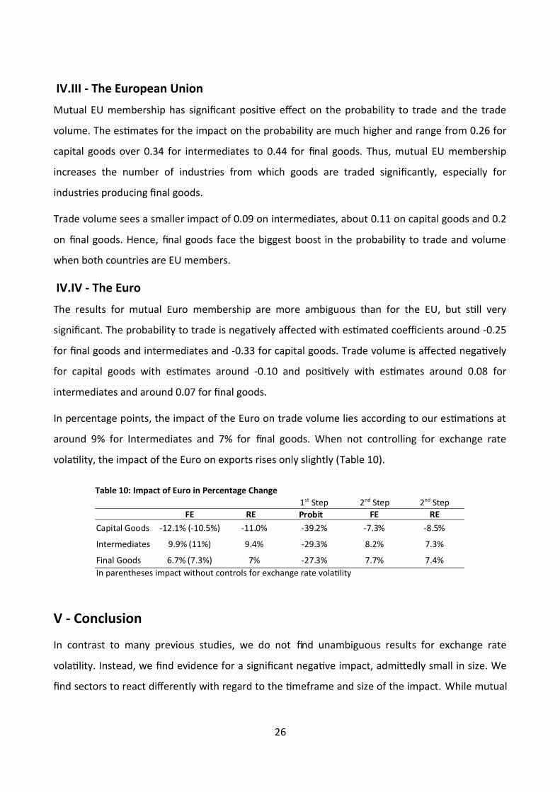
IV.III - The European Union
Mutual EU membership has signifcant positive effect on the probability to trade and the trade
volume. The estimates for the impact on the probability are much higher and range from 0.26 for
capital goods over 0.34 for intermediates to 0.44 for fnal goods. Thus, mutual EU membership
increases the number of industries from which goods are traded signifcantly, especially for
industries producing fnal goods.
Trade volume sees a smaller impact of 0.09 on intermediates, about 0.11 on capital goods and 0.2
on fnal goods. Hence, fnal goods face the biggest boost in the probability to trade and volume
when both countries are EU members.
IV.IV - The Euro
The results for mutual Euro membership are more ambiguous than for the EU, but still very
signifcant. The probability to trade is negatively affected with estimated coefficients around -0.25
for fnal goods and intermediates and -0.33 for capital goods. Trade volume is affected negatively
for capital goods with estimates around -0.10 and positively with estimates around 0.08 for
intermediates and around 0.07 for fnal goods.
In percentage points, the impact of the Euro on trade volume lies according to our estimations at
around 9% for Intermediates and 7% for fnal goods. When not controlling for exchange rate
volatility, the impact of the Euro on exports rises only slightly (Table 10).
V - Conclusion
In contrast to many previous studies, we do not fnd unambiguous results for exchange rate
volatility. Instead, we fnd evidence for a signifcant negative impact, admitedly small in size. We
fnd sectors to react differently with regard to the timeframe and size of the impact. While mutual
26
Table 10: Impact of Euro in Percentage Change
FE RE FE RECapital Goods -12.1% (-10.5%) -11.0% -39.2% -7.3% -8.5%
Intermediates 9.9% (11%) 9.4% -29.3% 8.2% 7.3%
Final Goods 6.7% (7.3%) 7% -27.3% 7.7% 7.4%In parentheses impact without controls for exchange rate volatility
1st Step 2nd Step 2nd StepProbit
EU membership promotes trade via the extensive and intensive margin for most goods, Euro
membership does so only via the intensive margin and not for capital goods. This is evidence for a
pronounced specialization process in the Eurozone at the industry level, which results in countries
exporting goods from less industries, but higher overall volumes. According to our results, the
effect is slightly stronger for intermediates than fnal goods.
Negative trade effects for the Euro for capital goods can probably be atributed to the massive
capital flows with the start of the Euro from members in central Europe to the periphery, that
fuelled a consumption/housing bubble in the periphery and led to less investments in capital
goods in the centre and the periphery of the Eurozone and therefore lower trade of capital goods
between the Eurozone members.
The introduction of controls for frm heterogeneity and sample selection bias only very slightly
affects the results. Nonetheless, extensive and intensive margin are affected very differently by
our variables of interest.
V.I - Policy Implications
Policy implications stemming from our results are manifold. Policymakers should keep in mind,
that currency unions come at great costs with regard to the flexibility of the domestic monetary
policy, but positive trade effects may be very limited and not for all types of goods. The
elimination of exchange rate volatility can also be achieved by a fxed peg. Although we fnd trade
effects to be small, it still may be the beter choice to avoid negative impacts as experienced
currently in Eurozone and grants greater flexibility.
The question whether or not stabilizing the exchange rate is a desirable objective for policymakers
is unclear and it is also unclear to which extent the real exchange rate is a variable that
policymakers should be able to influence or actually can influence, besides establishing a currency
union, a fxed peg or Dollarization (Eichengreen 2007; Rodrik 2008).
27

VI - Bibliography
Anderson, J.E. & van Wincoop, E., 2003. Gravity with Gravitas: A Solution to the Border Puzzle.
American Economic Review, 93(1), pp.170 - 192.
Anderson, J.E. & van Wincoop, E., 2004. Trade Costs. Journal of Economic Literature, 42(3), pp.691
- 751.
Anderson, J.E. & Yotov, Y.V., 2010. The Changing Incidence of Geography. American Economic
Review, 100(5), pp.2157 - 86.
Auboin, M. & Ruta, M., 2011. The Relationship Between Exchange Rates and International Trade: A
Review of Economic Literature. WTO Working Paper, 17(October).
Baccheta, P. & van Wincoop, E., 2000. Does Exchange-Rate Stability Increase Trade and Welfare?
American Economic Review, 90(5), pp.1093 - 1109.
Bahmani-Oskooee, M. & Hanafah, H., 2011. Exchange-rate volatility and industry trade between
the U.S. and Malaysia. Research in International Business and Finance, 25(2), pp.127 - 155.
Bahmani-Oskooee, M. & Hegerty, S.W., 2007. Exchange rate volatility and trade flows: a review
article. Journal of Economic Studies, 34(3), pp.211 - 255.
Bahmani-Oskooee, M. & Hegerty, S.W., 2008. Exchange-rate risk and U.S.-Japan trade: Evidence
from industry level data. Journal of the Japanese and International Economies, 22(4), pp.518 -
534.
Bahmani-Oskooee, M. & Wang, Y., 2007. United States-China Trade At The Commodity Level And
The Yuan-Dollar Exchange Rate. Contemporary Economic Policy, 25(3), pp.341 - 361.
Baldwin, R., 2006. The Euro’s Trade Effect. ECB Working Paper Series, 594.
Baldwin, R. & Krugman, P., 1989. Persistent Trade Effects of Large Exchange Rate Shocks. The
Quarterly Journal of Economics, 104(4), pp.635 - 54.
Baldwin, R., Skudelny, F. & Taglioni, D., 2005. Trade effects of the euro - evidence from sectoral
data. European Central Bank, 446.
I

Barkoulas, J.T., Baum, C.F. & Caglayan, M., 2002. Exchange rate effects on the volume and
variability of trade flows. Journal of International Money and Finance, 21(4), pp.481 - 496.
Baron, D.P., 1976. Fluctuating Exchange Rates and the Pricing of Exports. Economic Inquiry, 14(3),
pp.425 - 38.
Baum, C.F. & Caglayan, M., 2010. On the sensitivity of the volume and volatility of bilateral trade
flows to exchange rate uncertainty. Journal of International Money and Finance, 29(1), pp.79-
93.
Baum, C.F., Caglayan, M. & Ozkan, N., 2004. Nonlinear effects of exchange rate volatility on the
volume of bilateral exports. Journal of Applied Econometrics, 19(1), pp.1 - 23.
Berger, H. & Nitsch, V., 2008. Zooming out: The trade effect of the euro in historical perspective.
Journal of International Money and Finance, 27(8), pp.1244 - 1260.
Bergin, P. & Tchakarov, I., 2003. Does Exchange Rate Risk Mater for Welfare? Computing in
Economics and Finance, 61.
Berman, N., Martin, P. & Mayer, T., 2009. How do different exporters react to exchange rate
changes? Theory, empirics and aggregate implications. CEPR Discussion Papers, 7493.
Boug, P. & Fagereng, A., 2010. Exchange rate volatility and export performance: a cointegrated
VAR approach. Applied Economics, 42(7), pp.851 - 864.
Broll, U. & Eckwert, B., 1999. Exchange Rate Volatility and International Trade. Southern Economic
Journal, 66(1), pp.178 - 185.
Broll, U., Wahl, J.E. & Wong, W.-K., 2006. Elasticity of risk aversion and international trade.
Economics Leters, 92(1), pp.126 - 130.
Byrne, J.P., Darby, J. & MacDonald, R., 2008. US trade and exchange rate volatility: A real sectoral
bilateral analysis. Journal of Macroeconomics, 30(1), pp.238 - 259.
Caglayan, M. & Di, J., 2010. Does Real Exchange Rate Volatility Affect Sectoral Trade Flows?
Southern Economic Journal, 77(2), pp.313-335.
Canzoneri, M.B. & Clark, P.B., 1984. The effects of exchange rate variability on output and
employment. International Finance Discussion Papers, 240.
II
Chit, M.M., Rizov, M. & Willenbockel, D., 2010. Exchange Rate Volatility and Exports: New
Empirical Evidence from the Emerging East Asian Economies. The World Economy, 33(2),
pp.239 - 263.
Cho, G., Sheldon, I.M. & McCorriston, S., 2002. Exchange Rate Uncertainty and Agricultural Trade.
American Journal of Agricultural Economics, 84(4), pp.931 - 42.
Clark, P.B., Sadikov, A.M., et al., 2004. A New Look at Exchange Rate Volatility and Trade Flows.
IMF Occasional Papers, 235.
Clark, P.B., Tamirisa, N., et al., 2004. Exchange Rate Volatility and Trade Flows - Some New
Evidence. International Monetary Fund Occasional Paper, No. 235.
Clark, P.B., 1973. Uncertainty, exchange risk, and the level of international trade. Economic
Inquiry, 11(3), pp.302-313.
Coter, J. & Bredin, D., 2011. Real and Nominal Foreign Exchange Volatility Effects on Exports – The
Importance of Timing.
Crozet, M., Koenig, P. & Rebeyrol, V., 2008. Exporting to Insecure Markets: a Firm-Level Analysis.
Cushman, D.O., 1986. Has exchange risk depressed international trade? The impact of third-
country exchange risk. Journal of International Money and Finance, 5(3), pp.361 - 379.
Cushman, D.O., 1983. The effects of real exchange rate risk on international trade. Journal of
International Economics, 15(August), pp.45 - 63.
Côté, A., 1994. Exchange Rate Volatility and Trade: A Survey. EconWPA, 9406001.
Coric, B. & Pugh, G., 2010. The effects of exchange rate variability on international trade: a meta-
regression analysis. Applied Economics, 42(20), pp.2631 - 2644.
Dixit, A.K., 1989. Entry and Exit Decisions under Uncertainty. Journal of Political Economy, 97(3),
pp.620 - 38.
Eichengreen, B., 2007. The Real Exchange Rate and Economic Growth. Commission on Growth and
Development Working Paper, 4(World Bank.).
Eicher, T.S. & Henn, C., 2011. One Money, One Market: A Revised Benchmark. Review of
International Economics, 19(3), pp.419 - 435.
III

Flam, H. & Nordström, H., 2007. Explaining large euro effects on trade: the extensive margin and
vertical specialization. Manuscript, Institute for International Economic Studies, Stockholm
University.
Franke, G., 1991. Exchange rate volatility and international trading strategy. Journal of
International Money and Finance, 10(2), pp.292 - 307.
De Grauwe, P., 1988. Exchange Rate Variability and the Slowdown in Growth of International
Trade. IMF Staff Papers, 35(1), pp.63 - 84.
Grier, K.B. & Smallwood, A.D., 2007. Uncertainty and Export Performance: Evidence from 18
Countries. Journal of Money, Credit and Banking, 39(4), pp.965 - 979.
Havránek, T., 2010. Rose effect and the euro: is the magic gone? Review of World Economics,
146(2), pp.241-261.
Helpman, E., Melitz, M. & Rubinstein, Y., 2008. Estimating Trade Flows: Trading Partners and
Trading Volumes. The Quarterly Journal of Economics, 123(2), pp.441-487.
Hondroyiannis, G. et al., 2008. Some Further Evidence on Exchange-Rate Volatility and Exports.
Review of World Economics, 144(1), pp.151 - 180.
Hooper, P. & Kohlhagen, S.W., 1978. The effect of exchange rate uncertainty on the prices and
volume of international trade. Journal of International Economics, 8(4), pp.483 - 511.
Huchet-Bourdon, M. & Korinek, J., 2011. To What Extent Do Exchange Rates and their Volatility
Affect Trade? OECD Trade Policy Working Papers, 119, p.45.
Klein, M.W. & Shambaugh, J.C., 2006. Fixed exchange rates and trade. Journal of International
Economics, 70(2), pp.359 - 383.
Krugman, P., 1986. Pricing to Market when the Exchange Rate Changes. NBER Working Paper,
1926.
Makin, J.H., 1978. Portfolio Theory and the Problem of Foreign Exchange Risk. Journal of Finance,
33(2), pp.517 - 34.
McKenzie, M.D., 1999. The Impact of Exchange Rate Volatility on International Trade Flows.
Journal of Economic Surveys, 13(1), pp.71 - 106.
IV

Mongelli, F.P. & Vega, J.L., 2006. What Effects is EMU Having on the Euro Area and Its Member
Countries?: An Overview. ECB Working Paper Series, (599).
Obstfeld, M. & Rogoff, K., 1998. Risk and Exchange Rates. NBER Working Paper Series, 6694.
Ozturk, I., 2006. Exchange Rate Volatility and Trade: A Literature Survey. International Journal of
Applied Econometrics and Quantitative Studies, 3(1).
Ozturk, I. & Kalyoncu, H., 2009. Exchange Rate Volatility and Trade : An Empirical Investigation
from Cross-country Comparison. African Development Review, 21(3), pp.499-513.
Rahman, S. & Serletis, A., 2009. The effects of exchange rate uncertainty on exports. Journal of
Macroeconomics, 31(3), pp.500 - 507.
Rodrik, D., 2008. The Real Exchange Rate and Economic Growth. Brookings Papers on Economic
Activity, Fall 2008, pp.365 - 439.
Rose, A.K., 2000. One Money, One Market: Estimating the Effect of Common Currencies on Trade.
Economic Policy, 15(30), pp.7-46.
Rose-Ackerman, S., 1999. Corruption and Government: Causes, Consequences, and Reform,
Cambridge University Press.
Santos Silva, J.M.C. & Tenreyro, S., 2010. Currency Unions in Prospect and Retrospect. Annual
Review of Economics, 2(1), pp.51 - 74.
United Nations Department of Economic and Social Affairs, 2007. Future revision of the
Classification by Broad Economic Categories (BEC),
Viaene, J.-M. & de Vries, C.G., 1992. International trade and exchange rate volatility. European
Economic Review, 36(6), pp.1311 - 1321.
Wang, K.-L. & Barret, C.B., 2007. Estimating the Effects of Exchange Rate Volatility on Export
Volumes. Journal of Agricultural and Resource Economics, 32(02).
Wang, K.-L., Fawson, C. & Barret, C.B., 2002. An Assessment of Empirical Model Performance
When Financial Market Transactions Are Observed at Different Data Frequencies: An
Application to East Asian Exchange Rates. Review of Quantitative Finance and Accounting,
19(2), pp.111 - 29.
V

Wei, S.-J., 1999. Currency hedging and goods trade. European Economic Review, 43(7), pp.1371 -
1394.
VI

VII - Appendix
VII
Figure 2: Share of total exports by BEC category, 1996-2010
111 112 121 122 210 220 310 321 322 410 420 510 521 522 530 610 620 630 7000
0.05
0.1
0.15
0.2
0.25
0.3
Capital Goods Intermediates Final Goods

VIII
Figure 3: Log of Total Trade Volumes
01/96 09/96 05/97 01/98 09/98 05/99 01/00 09/00 05/01 01/02 09/02 05/03 01/04 09/04 05/05 01/06 09/06 05/07 01/08 09/08 05/09 01/10 09/109.5
10.5
11.5
12.5
Capital Goods
Intermediates
Final Goods

Table 11: Fixed Effects Regressions - Capital Goods
Table 12: Fixed Effects Regressions - Intermediates
IX
(1) (2) (3) (4) (5) (6)0.506*** 0.560*** 0.473*** 0.606*** 0.493*** 0.631***(0.0325) (0.0131) (0.0159) (0.0104) (0.0199) (0.0174)
0.0891*** 0.0890*** 0.101*** 0.103*** 0.0936***(0.00898) (0.00898) (0.00888) (0.00887) (0.00897)0.0939*** 0.0939*** 0.104*** 0.100*** 0.101***(0.0116) (0.0116) (0.0115) (0.0115) (0.0116)
-2.435*** -2.450*** -2.559*** -2.659***(0.285) (0.284) (0.284) (0.284)
-2.560*** -2.534*** -2.722*** -2.866***(0.339) (0.338) (0.338) (0.337)
-1.865*** -1.875*** -1.993*** -2.203***(0.282) (0.282) (0.282) (0.280)
-0.615** -0.613** -0.738** -0.648**(0.298) (0.298) (0.297) (0.298)
-0.0911** -0.115*** -0.0910** -0.0904**(0.0394) (0.0383) (0.0394) (0.0394)0.0820** 0.0892*** 0.0820** 0.0809**(0.0349) (0.0337) (0.0349) (0.0349)-0.0136 -0.0217 -0.0139 -0.0122(0.0409) (0.0407) (0.0409) (0.0409)0.0191 0.0192 0.0195 0.0185
(0.0301) (0.0299) (0.0301) (0.0301)Obs. 1,045,992 1,045,992 1,057,399 1,073,052 1,045,992 1,045,992
0.113 0.113 0.116 0.119 0.113 0.113
GDPijt
EUijt
Euroijt
Volatilityijt
L1.Volatilityijt
L2.Volatilityijt
L3.Volatilityijt
ExRateijt
L1.ExRateijt
L2.ExRateijt
L3.ExRateijt
R2
Standard errors in parentheses; signifcance levels: * 10% ** 5% ***1%
(1) (2) (3) (4) (5) (6)0.426*** 0.504*** 0.632*** 0.575*** 0.446*** 0.457***(0.0300) (0.0313) (0.0291) (0.0207) (0.0382) (0.0272)0.119*** 0.119*** 0.138*** 0.143*** 0.113***(0.0160) (0.0160) (0.0159) (0.0159) (0.0160)
-0.112*** -0.112*** -0.100*** -0.0923*** -0.101***(0.0207) (0.0207) (0.0206) (0.0204) (0.0207)
-2.805*** -2.923*** -2.656*** -3.091***(0.514) (0.513) (0.513) (0.512)
-3.485*** -3.520*** -3.286*** -3.879***(0.612) (0.612) (0.611) (0.610)
-3.528*** -3.459*** -3.370*** -3.965***(0.509) (0.508) (0.508) (0.505)
-1.468*** -1.455*** -1.323** -1.505***(0.531) (0.531) (0.530) (0.531)
-0.301*** -0.332*** -0.302*** -0.300***(0.0710) (0.0689) (0.0710) (0.0710)0.0499 0.0849 0.0499 0.0486
(0.0634) (0.0612) (0.0634) (0.0634)0.271*** 0.241*** 0.272*** 0.274***(0.0734) (0.0730) (0.0734) (0.0734)0.0825 0.0933* 0.0823 0.0809
(0.0547) (0.0544) (0.0547) (0.0547)Obs. 283,895 283,895 287,010 291,256 283,895 283,895
0.194 0.194 0.198 0.200 0.194 0.194
GDPijt
EUijt
Euroijt
Volatilityijt
L1.Volatilityijt
L2.Volatilityijt
L3.Volatilityijt
ExRateijt
L1.ExRateijt
L2.ExRateijt
L3.ExRateijt
R2
Standard errors in parentheses; signifcance levels: * 10% ** 5% ***1%
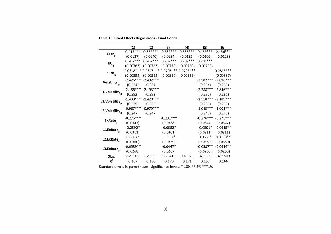
Table 13: Fixed Effects Regressions - Final Goods
X
(1) (2) (3) (4) (5) (6)0.417*** 0.352*** 0.639*** 0.538*** 0.439*** 0.456***(0.0127) (0.0140) (0.0134) (0.0132) (0.0109) (0.0128)0.202*** 0.202*** 0.209*** 0.209*** 0.205***(0.00787) (0.00787) (0.00778) (0.00780) (0.00785)0.0648*** 0.0647*** 0.0705*** 0.0722*** 0.0813***(0.00999) (0.00999) (0.00996) (0.00992) (0.00997)-2.426*** -2.492*** -2.502*** -2.896***
(0.234) (0.234) (0.234) (0.233)-2.186*** -2.193*** -2.288*** -2.846***
(0.282) (0.282) (0.282) (0.281)-1.438*** -1.420*** -1.518*** -2.189***
(0.235) (0.235) (0.235) (0.233)-0.967*** -0.979*** -1.045*** -1.001***
(0.247) (0.247) (0.247) (0.247)-0.276*** -0.291*** -0.276*** -0.275***(0.0347) (0.0338) (0.0347) (0.0347)-0.0592* -0.0582* -0.0591* -0.0615**(0.0311) (0.0301) (0.0311) (0.0311)0.0667* 0.0654* 0.0665* 0.0713**(0.0360) (0.0359) (0.0360) (0.0360)
-0.0589** -0.0447* -0.0587** -0.0614**(0.0268) (0.0267) (0.0268) (0.0268)
Obs. 879,509 879,509 889,410 902,978 879,509 879,5090.167 0.166 0.170 0.171 0.167 0.166
GDPijt
EUijt
Euroijt
Volatilityijt
L1.Volatilityijt
L2.Volatilityijt
L3.Volatilityijt
ExRateijt
L1.ExRateijt
L2.ExRateijt
L3.ExRateijt
R2
Standard errors in parentheses; signifcance levels: * 10% ** 5% ***1%