Exciton and Polariton BECDavid SnokeUniversity of Pittsburgh

on sale now:

Vince Hartwell

David Snoke

Zoltan Vörös

Nick Sinclair

Botao Zhang

Bridget Bertoni Ryan Balili

Chuan YangBryan Nelson Jeff Wuenschell

Annie Wang

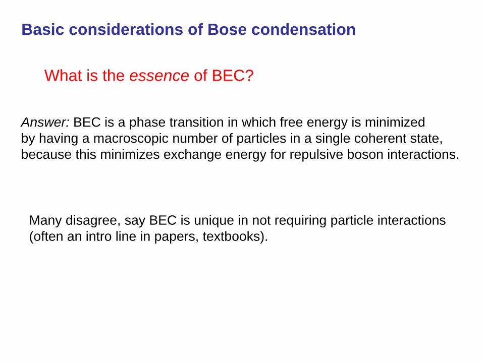
Basic considerations of Bose condensation

What is the essence of BEC?

Answer: BEC is a phase transition in which free energy is minimized by having a macroscopic number of particles in a single coherent state,because this minimizes exchange energy for repulsive boson interactions.

Many disagree, say BEC is unique in not requiring particle interactions(often an intro line in papers, textbooks).

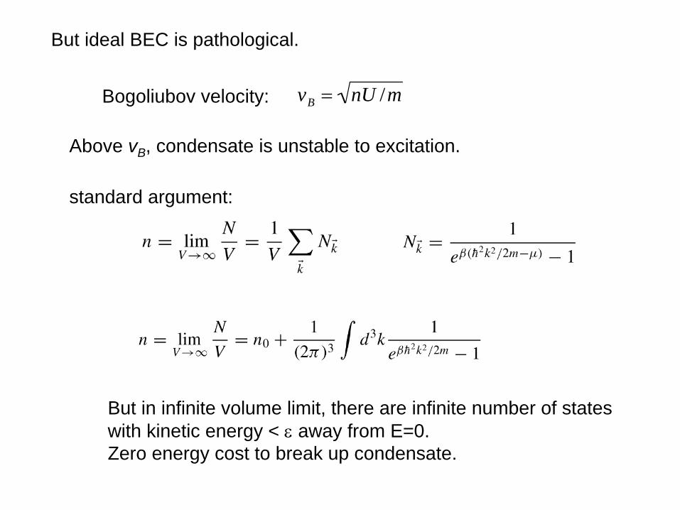
But ideal BEC is pathological.

Bogoliubov velocity: vB = nU /m

Above vB , condensate is unstable to excitation.

standard argument:

But in infinite volume limit, there are infinite number of stateswith kinetic energy < ε

away from E=0.Zero energy cost to break up condensate.

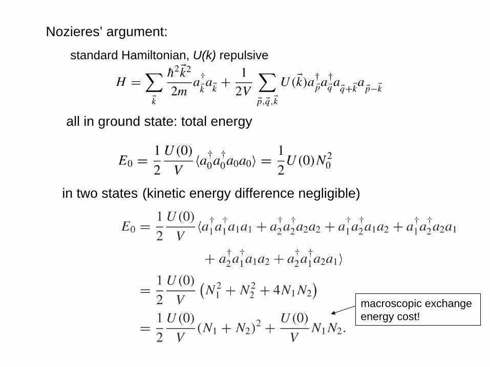
all in ground state: total energy

Nozieres’ argument:

standard Hamiltonian, U(k) repulsive

in two states (kinetic energy difference negligible)

macroscopic exchange energy cost!

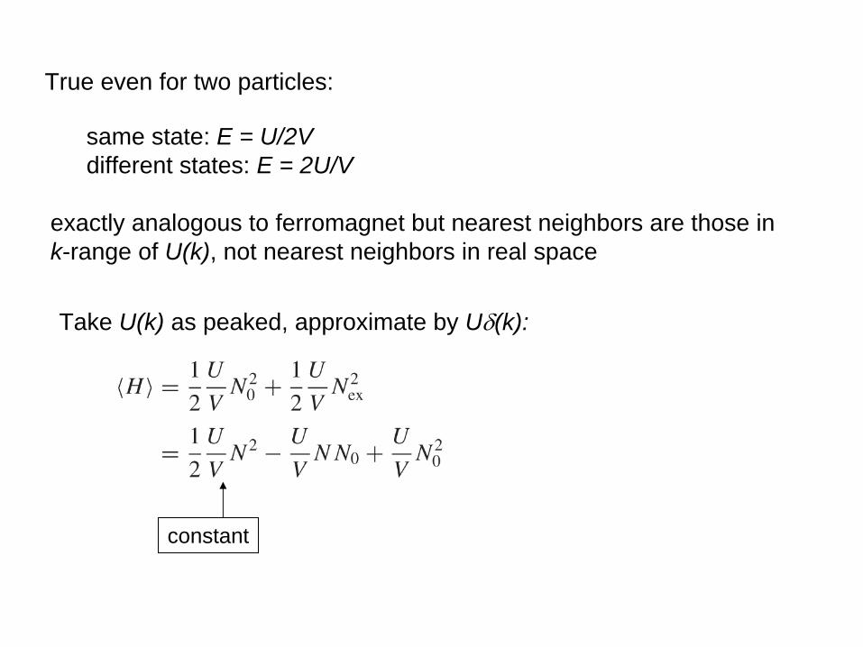
True even for two particles:

same state: E = U/2Vdifferent states: E = 2U/V

exactly analogous to ferromagnet but nearest neighbors are those ink-range of U(k), not nearest neighbors in real space

Take U(k) as peaked, approximate by Uδ(k):

constant

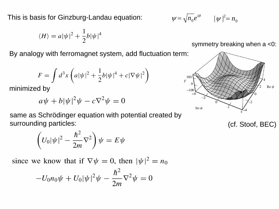
This is basis for Ginzburg-Landau equation:

By analogy with ferromagnet system, add fluctuation term:

minimized by

same as Schrödinger equation with potential created bysurrounding particles:

symmetry breaking when a <0:

(cf. Stoof, BEC)

ψ = n0eiθ |ψ |2= n0

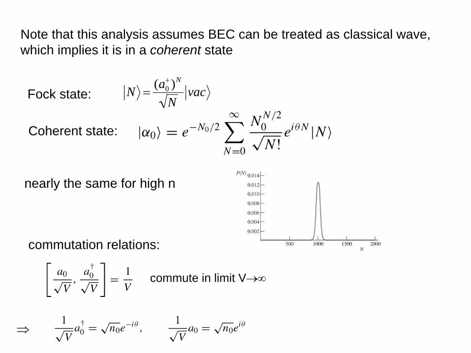
Note that this analysis assumes BEC can be treated as classical wave,which implies it is in a coherent state

Fock state:

Coherent state:

nearly the same for high n

commutation relations:

N =(a0

+)N

Nvac

commute in limit V→∞

⇒

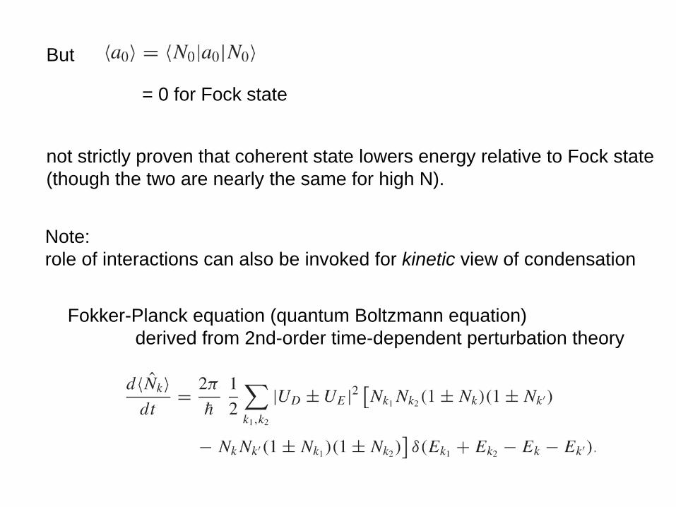
But

= 0 for Fock state

not strictly proven that coherent state lowers energy relative to Fock state(though the two are nearly the same for high N).

Note: role of interactions can also be invoked for kinetic view of condensation

Fokker-Planck equation (quantum Boltzmann equation)derived from 2nd-order time-dependent perturbation theory

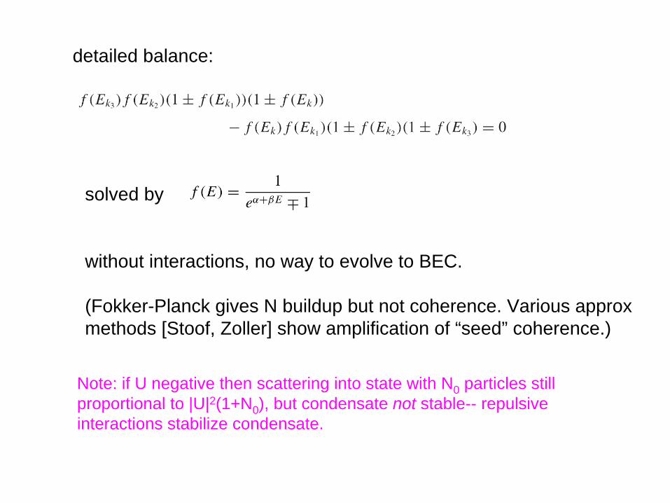
detailed balance:

solved by

without interactions, no way to evolve to BEC.

(Fokker-Planck gives N buildup but not coherence. Various approxmethods [Stoof, Zoller] show amplification of “seed” coherence.)

Note: if U negative then scattering into state with N0 particles still proportional to |U|2(1+N0 ), but condensate not stable-- repulsive interactions stabilize condensate.

General experimental implication of stability argument: key difference from laser (or coherent sound wave)

⇒ Resists multimode behavior (unless spatially non- overlapping)

“synchronization”“soliton-like” -- resists spatial dispersion

non-interacting waves can pass through each otherCondensate “sucks in” other condensates

laser: no direct interaction of modes, multimode lasing typicallysuppressed by absorption of other modes(more on this later...)

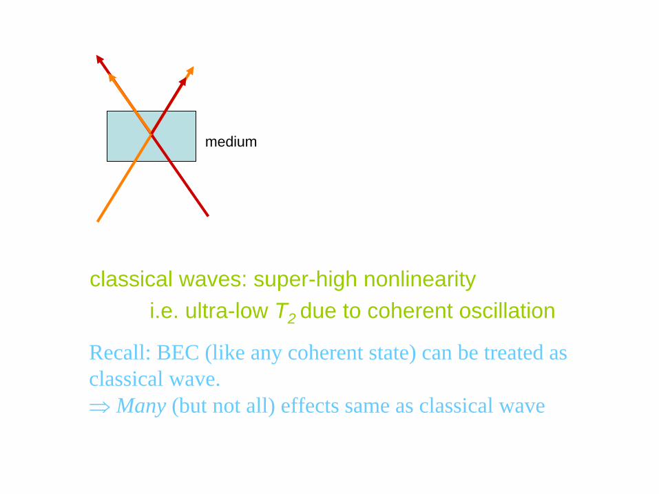
medium

classical waves: super-high nonlinearity

Recall: BEC (like any coherent state) can be treated asclassical wave. ⇒ Many (but not all) effects same as classical wave

i.e. ultra-low T2 due to coherent oscillation

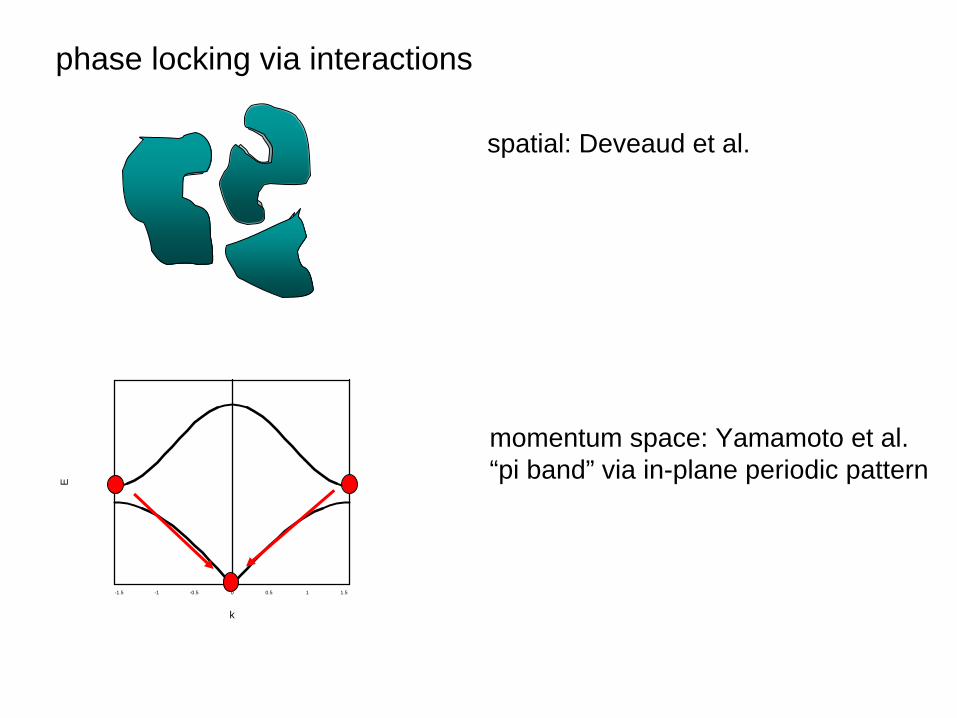
phase locking via interactions

spatial: Deveaud et al.

momentum space: Yamamoto et al.“pi band” via in-plane periodic pattern

-1.5 -1 -0.5 0 0.5 1 1.5

E

k

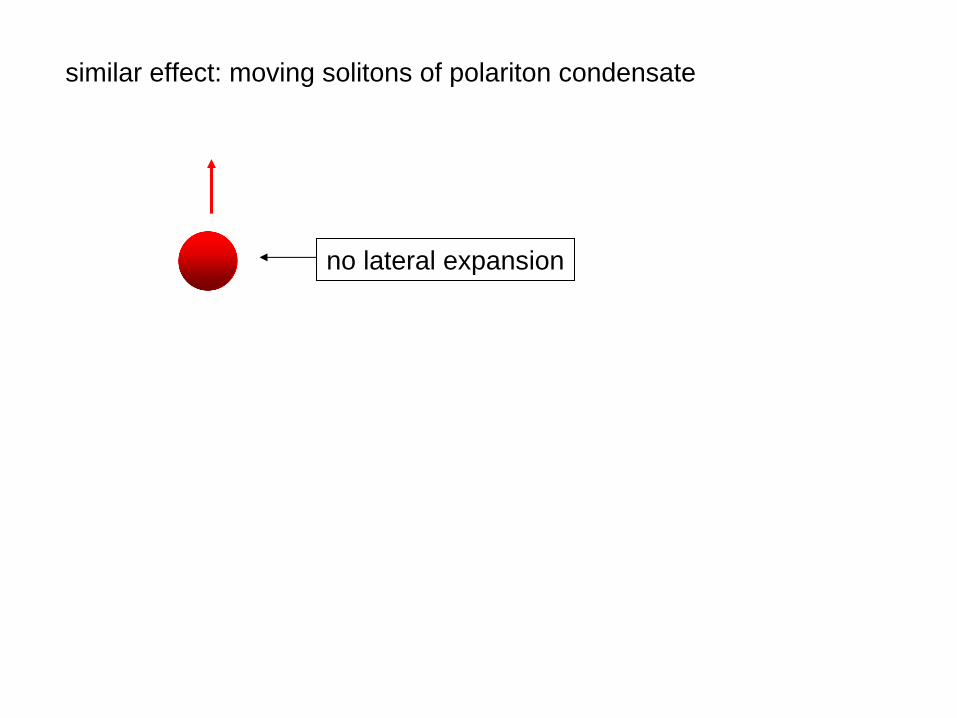
similar effect: moving solitons of polariton condensate

no lateral expansion

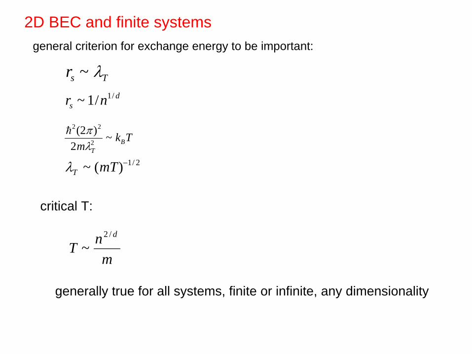
general criterion for exchange energy to be important:

rs ~ λT

rs ~ 1/n1/ d

h2(2π )2

2mλT2 ~ kBT

λT ~ (mT)−1/ 2

T ~ n2 / d

m

critical T:

generally true for all systems, finite or infinite, any dimensionality

2D BEC and finite systems

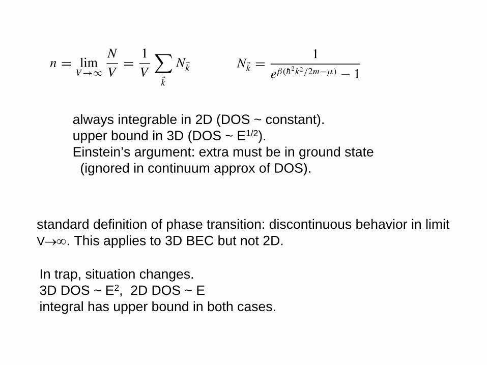
always integrable in 2D (DOS ~ constant).upper bound in 3D (DOS ~ E1/2).Einstein’s argument: extra must be in ground state (ignored in continuum approx of DOS).

standard definition of phase transition: discontinuous behavior in limitV→∞. This applies to 3D BEC but not 2D.

In trap, situation changes. 3D DOS ~ E2, 2D DOS ~ Eintegral has upper bound in both cases.

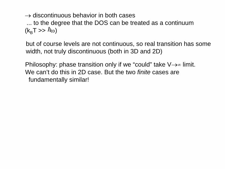
→ discontinuous behavior in both cases... to the degree that the DOS can be treated as a continuum(kB T >> ω) h

but of course levels are not continuous, so real transition has some width, not truly discontinuous (both in 3D and 2D)

Philosophy: phase transition only if we “could” take V→∞

limit. We can’t do this in 2D case. But the two finite cases are fundamentally similar!

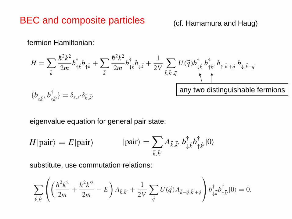
BEC and composite particles

fermion Hamiltonian:

any two distinguishable fermions

eigenvalue equation for general pair state:

substitute, use commutation relations:

(cf. Hamamura and Haug)

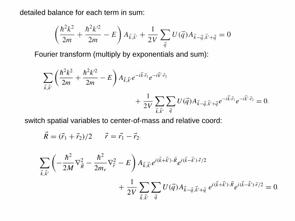
detailed balance for each term in sum:

Fourier transform (multiply by exponentials and sum):

switch spatial variables to center-of-mass and relative coord:

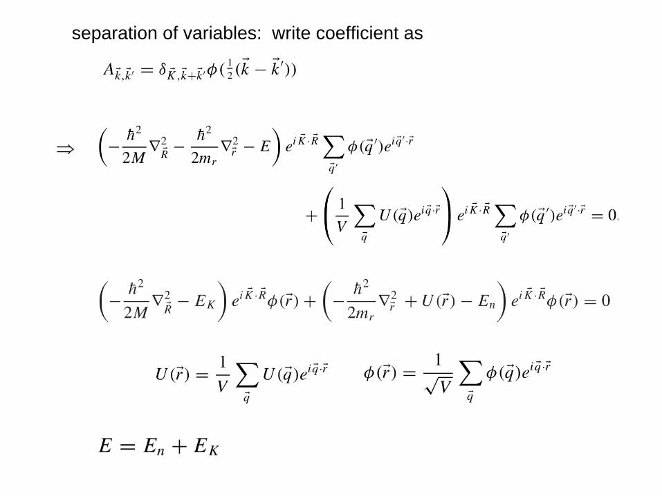
separation of variables: write coefficient as

⇒

⇒

where

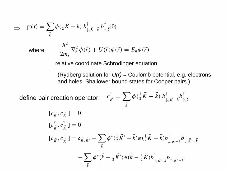
relative coordinate Schrodinger equation

define pair creation operator:

(Rydberg solution for U(r) = Coulomb potential, e.g. electrons and holes. Shallower bound states for Cooper pairs.)

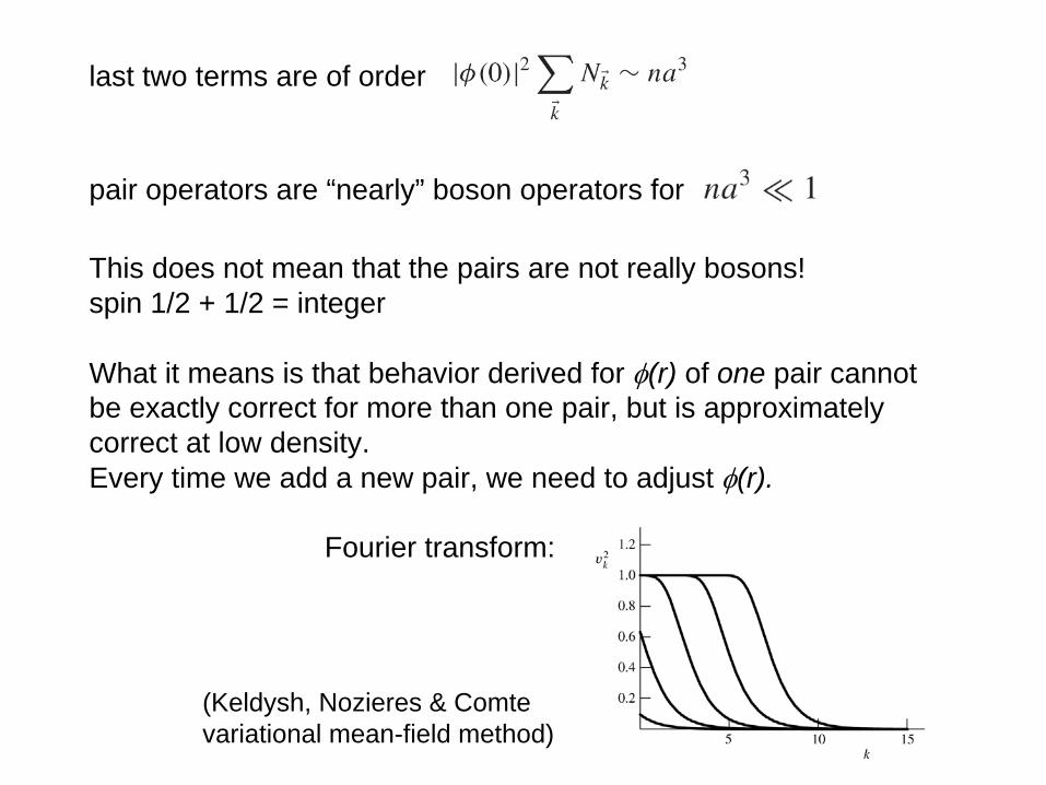
last two terms are of order

pair operators are “nearly” boson operators for

This does not mean that the pairs are not really bosons!spin 1/2 + 1/2 = integer

What it means is that behavior derived for φ(r) of one pair cannot be exactly correct for more than one pair, but is approximately correct at low density. Every time we add a new pair, we need to adjust φ(r).

Fourier transform:

(Keldysh, Nozieres & Comtevariational mean-field method)

BEC and BCS

pair creation operator

coherent state = condensate

two particle state:

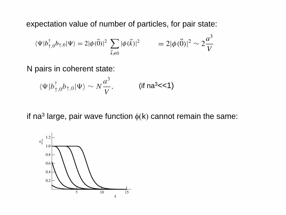
expectation value of number of particles, for pair state:

N pairs in coherent state:

(if na3<<1)

if na3 large, pair wave function φ(k)

cannot remain the same:

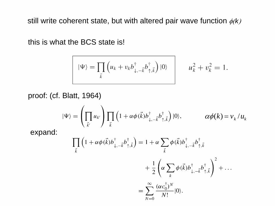
still write coherent state, but with altered pair wave function φ(k)

this is what the BCS state is!

proof: (cf. Blatt, 1964)

expand:

αφ(k) = vk /uk

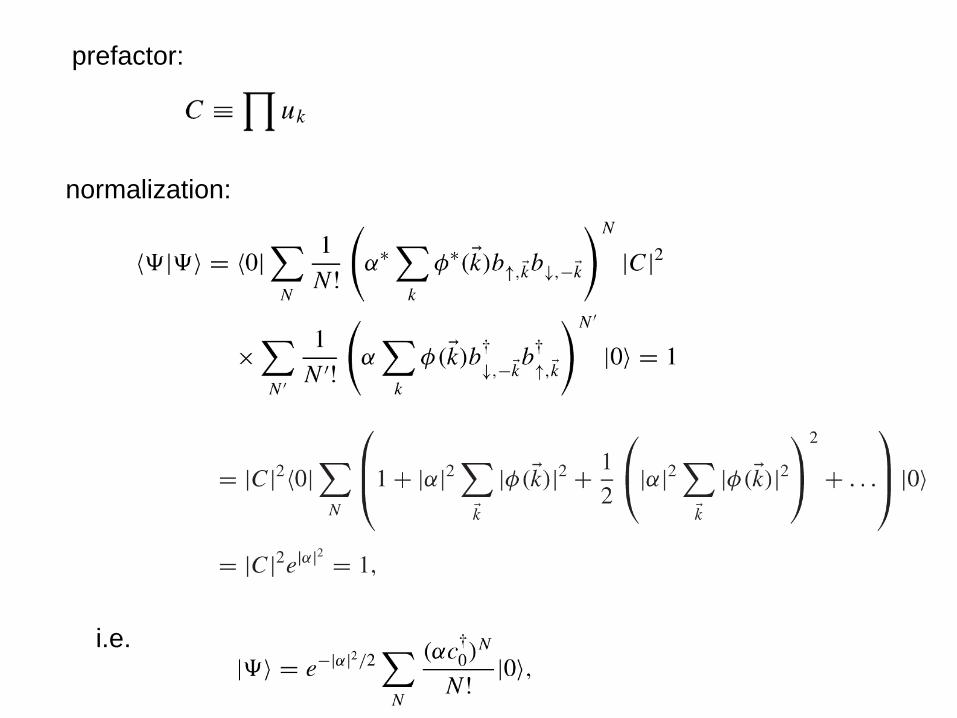
prefactor:

normalization:

i.e.

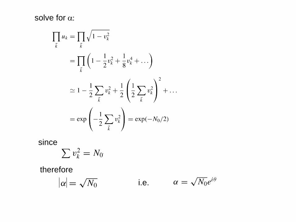
solve for α:

since

thereforei.e.

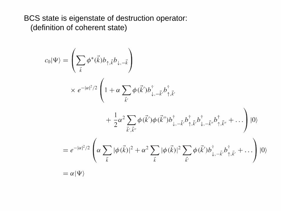
BCS state is eigenstate of destruction operator:(definition of coherent state)

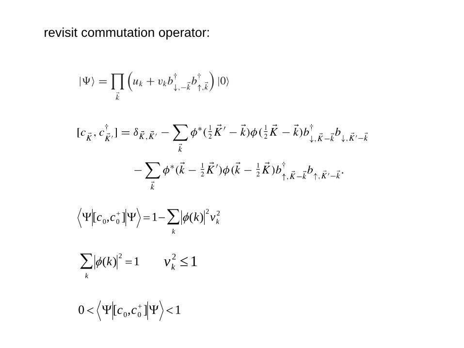
revisit commutation operator:

Ψ[c0,c0+]Ψ =1− φ(k) 2vk

2

k∑

φ(k) 2 =1k

∑ vk2 ≤1

0 < Ψ[c0,c0+]Ψ <1

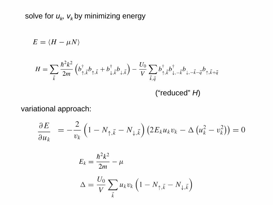
solve for uk , vk by minimizing energy

(“reduced” H)

variational approach:

⇒

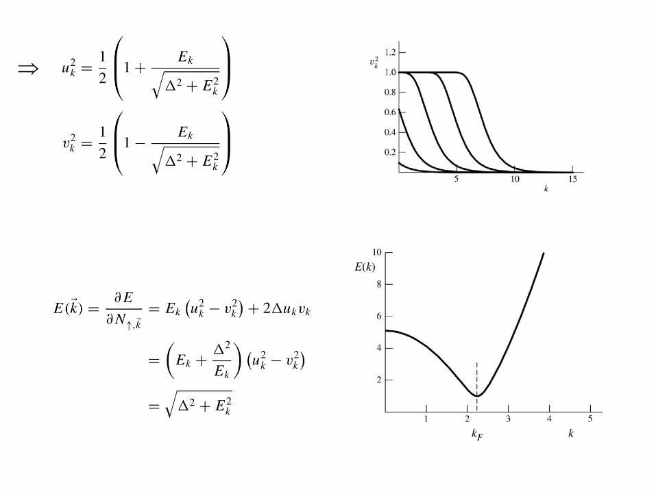
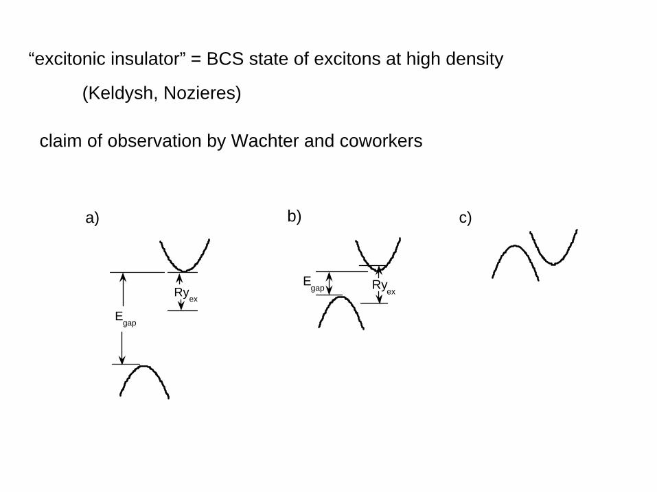
“excitonic insulator” = BCS state of excitons at high density

(Keldysh, Nozieres)

claim of observation by Wachter and coworkers

Egap

Ryex

a)

Ryex

b)

Egap

c)

QuickTime™ and a decompressor

are needed to see this picture.

resistivity vs. gap tuning

Wachter et al., narrow band gapsemiconductor, gap tuned by stress

coherence?

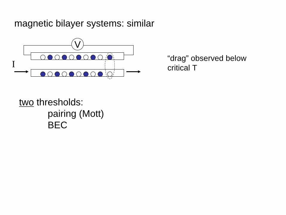
magnetic bilayer systems: similar

two thresholds: pairing (Mott)BEC

“drag” observed belowcritical TI

V

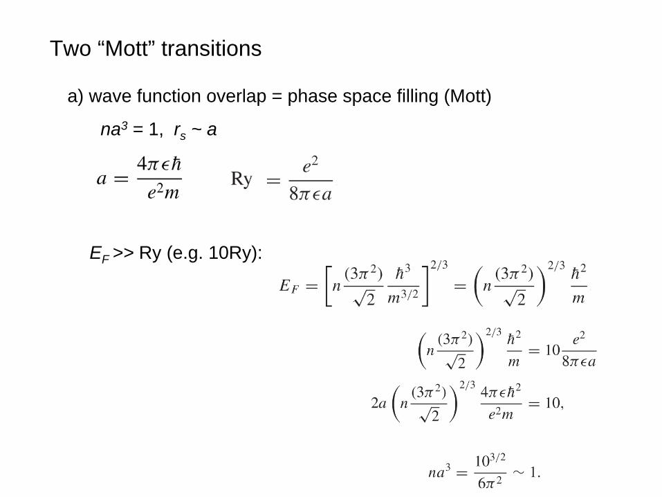
Two “Mott” transitions

a) wave function overlap = phase space filling (Mott)

na3 = 1, rs ~ a

EF >> Ry (e.g. 10Ry):

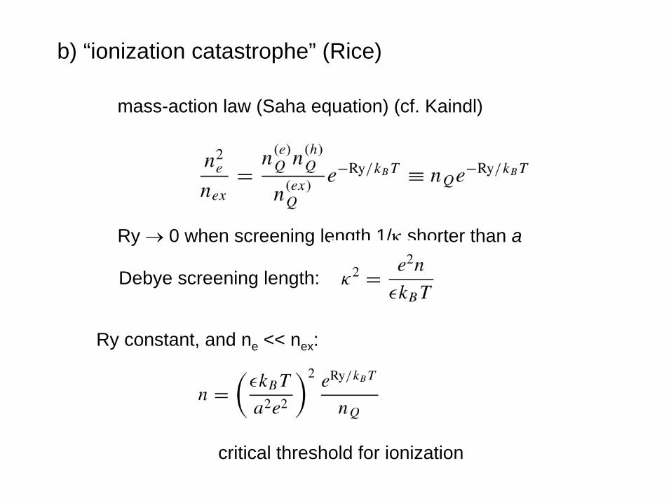
b) “ionization catastrophe” (Rice)

mass-action law (Saha equation) (cf. Kaindl)

Ry constant, and ne << nex :

Ry → 0 when screening length 1/κ

shorter than a

Debye screening length:

critical threshold for ionization

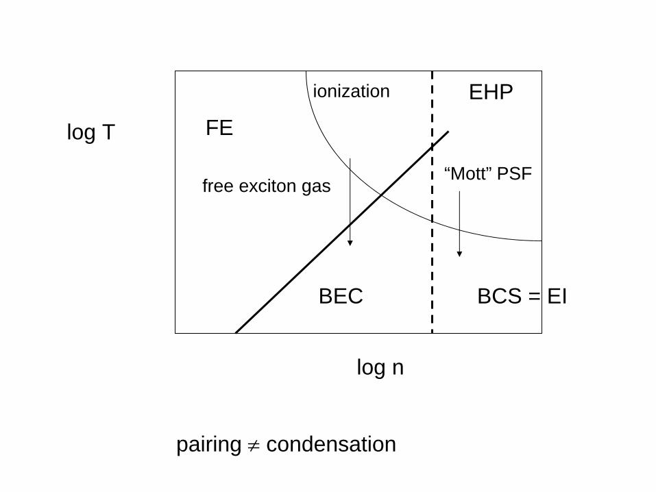
log n

log T

“Mott” PSF

BEC

ionization

free exciton gas

BCS = EI

pairing ≠

condensation

EHPFE

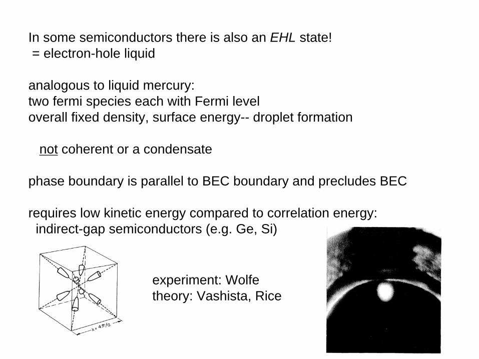
In some semiconductors there is also an EHL state!= electron-hole liquid

analogous to liquid mercury:two fermi species each with Fermi leveloverall fixed density, surface energy-- droplet formation

not coherent or a condensate

phase boundary is parallel to BEC boundary and precludes BEC

requires low kinetic energy compared to correlation energy:indirect-gap semiconductors (e.g. Ge, Si)

experiment: Wolfetheory: Vashista, Rice

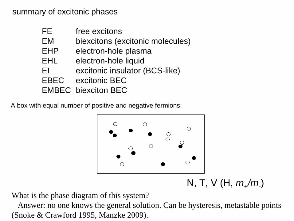
summary of excitonic phases

FE free excitonsEM biexcitons (excitonic molecules)EHP electron-hole plasmaEHL electron-hole liquidEI excitonic insulator (BCS-like)EBEC excitonic BECEMBEC biexciton BEC

A box with equal number of positive and negative fermions:

N, T, V (H, m+ /m- )What is the phase diagram of this system?

Answer: no one knows the general solution. Can be hysteresis, metastable points(Snoke & Crawford 1995, Manzke 2009).

Prehistory of exciton BEC

Early focus was on bulk semiconductors with deeply bound excitons(Rydberg ~ 100 meV)

•nearly impossible to exceed Mott density with 3D tightly bound (~ 5Å)excitons

•direct gap semiconductors: no electron-hole liquid (EHL) phase

• in principle can have BEC in indirect-gap semiconductors on shorttime scales (e.g. diamond, Gonokami)

early, independent predictions: Moskalenko 1959, Blatt 1962

early mean-field theory: Keldysh and Kozlov, 1967 Nozieres and Comte, 1982

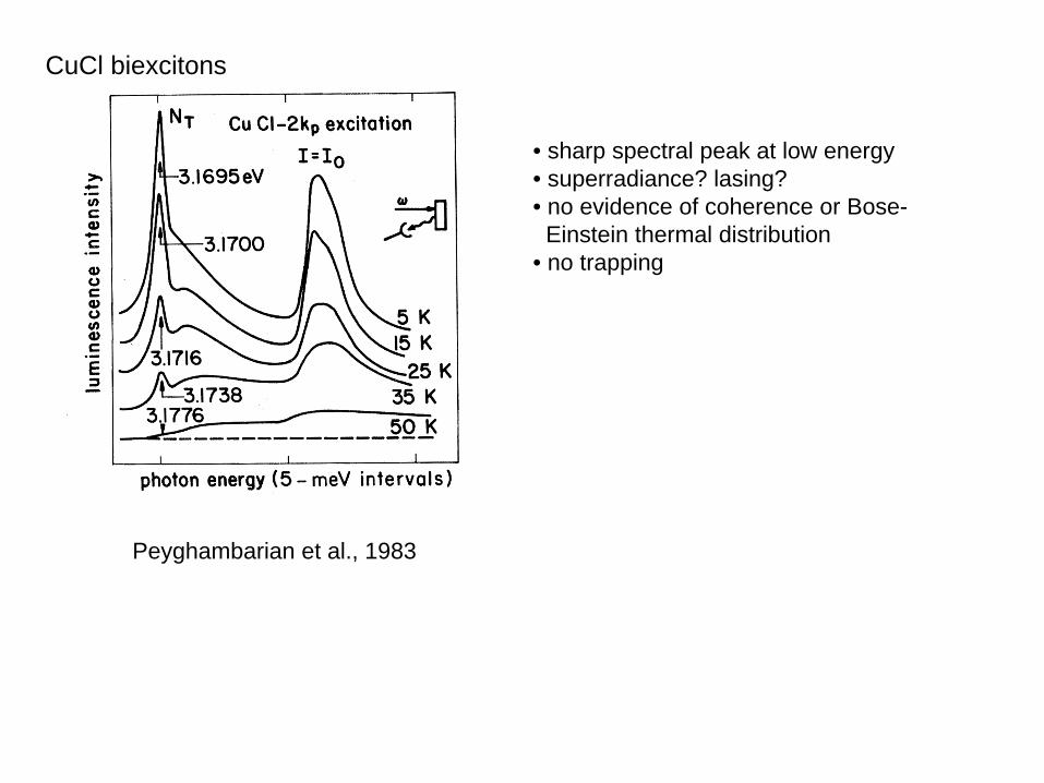
Peyghambarian et al., 1983

CuCl biexcitons

• sharp spectral peak at low energy • superradiance? lasing?• no evidence of coherence or Bose-

Einstein thermal distribution• no trapping

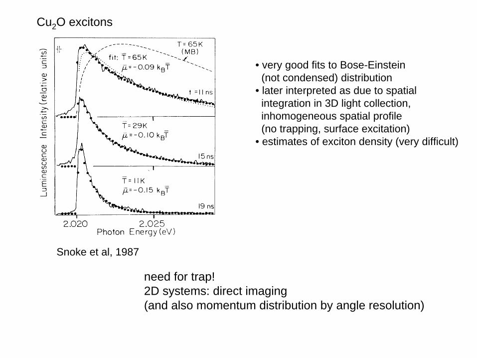
need for trap!2D systems: direct imaging (and also momentum distribution by angle resolution)

Cu2 O excitons

Snoke et al, 1987

• very good fits to Bose-Einstein (not condensed) distribution

• later interpreted as due to spatialintegration in 3D light collection,inhomogeneous spatial profile(no trapping, surface excitation)

• estimates of exciton density (very difficult)

Exciton and Polariton BECLecture 2

on sale now:

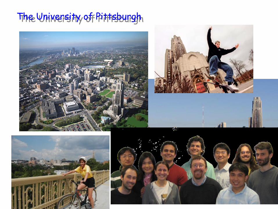
The University of PittsburghThe University of Pittsburgh

The Allegheny MountainsThe Allegheny Mountains

The Allegheny MountainsThe Allegheny Mountains

+ +

- -

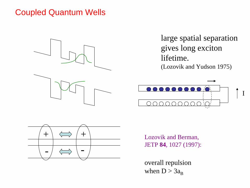
large spatial separation gives long excitonlifetime.(Lozovik and Yudson 1975)

Lozovik and Berman,JETP 84, 1027 (1997):

overall repulsionwhen D > 3aB

Coupled Quantum Wells

I

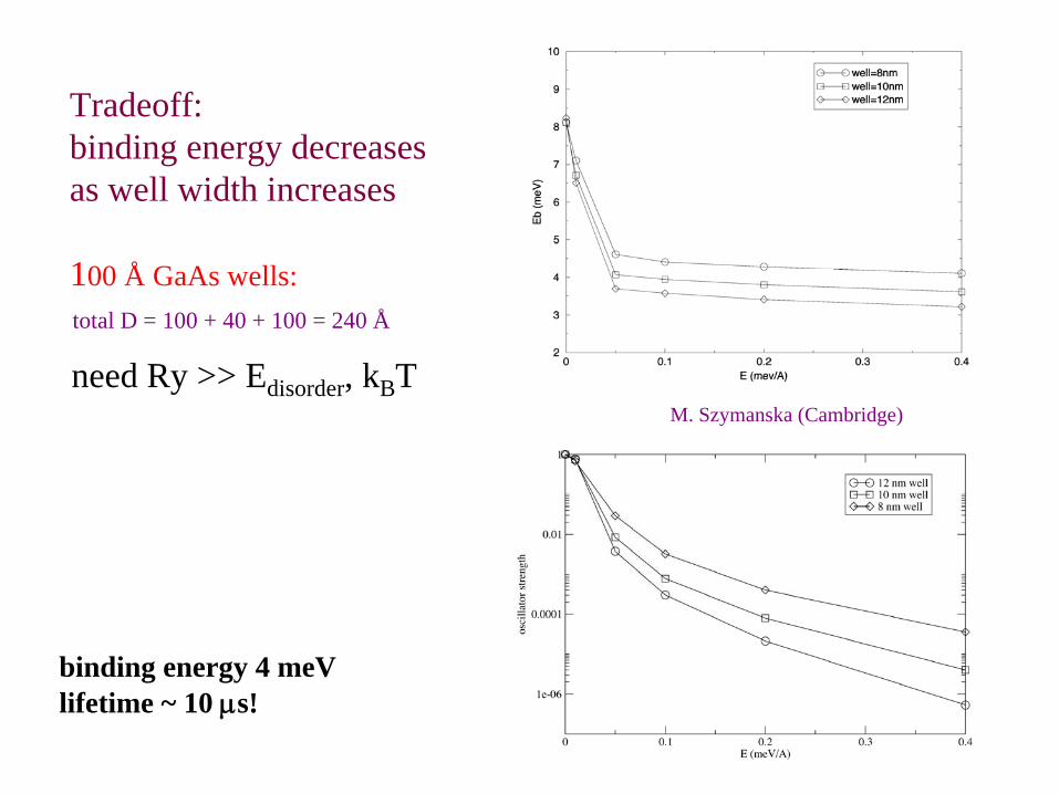
Tradeoff:binding energy decreasesas well width increases

100 Å GaAs wells:

M. Szymanska (Cambridge)

binding energy 4 meVlifetime ~ 10 μs!

total D = 100 + 40 + 100 = 240 Å

need Ry >> Edisorder , kB T

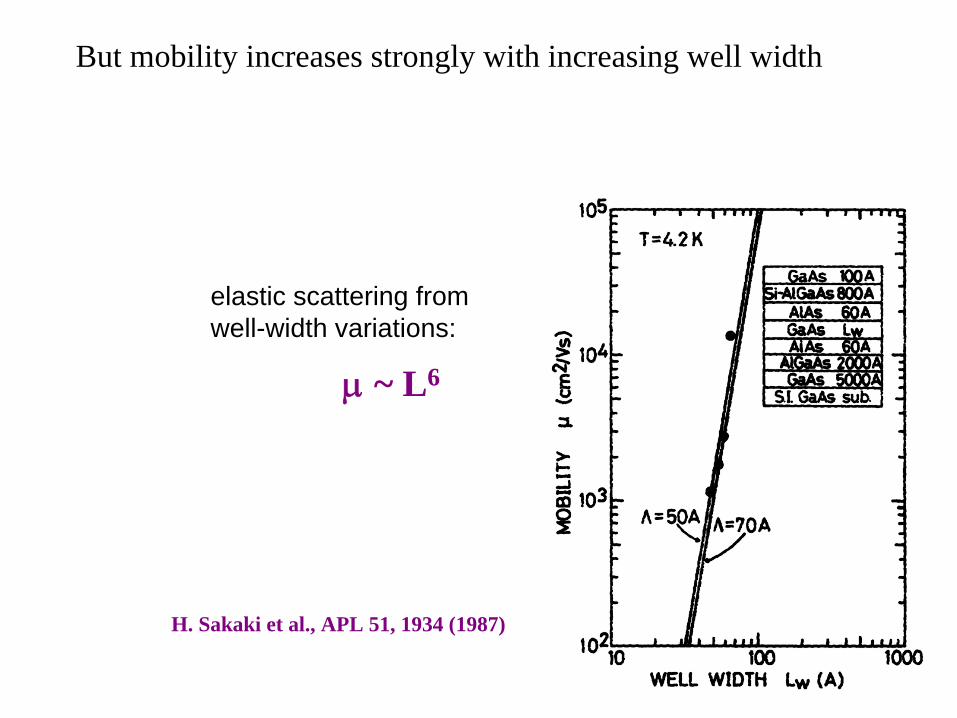
But mobility increases strongly with increasing well width

H. Sakaki et al., APL 51, 1934 (1987)

μ

~ L6

elastic scattering fromwell-width variations:

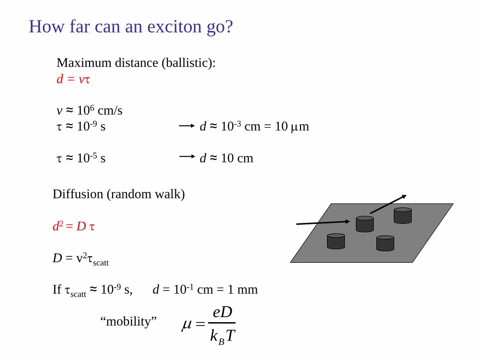
Maximum distance (ballistic):d = vτ

v ≈

106 cm/sτ

≈

10-9 s d ≈

10-3 cm = 10 μm

τ

≈

10-5 s d ≈

10 cm

How far can an exciton go?

Diffusion (random walk)

d2 = D τ

D = v2τscatt

If τscatt ≈

10-9 s, d = 10-1 cm = 1 mm

“mobility” μ =eDkBT

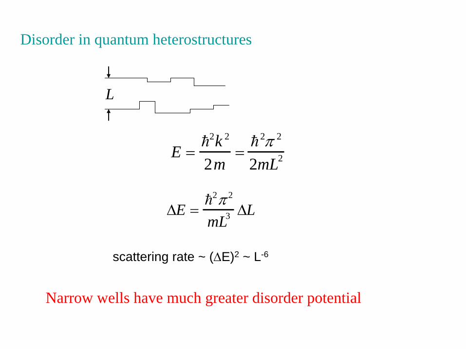
Disorder in quantum heterostructures

E =

h2k 2

2m=

h2π 2

2mL2

ΔE =

h2π 2

mL3 ΔL

L

Narrow wells have much greater disorder potential

scattering rate ~ (ΔE)2 ~ L-6

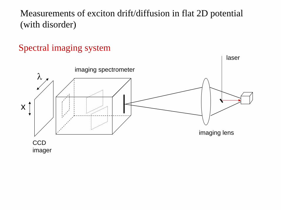
Spectral imaging system

λ

x

imaging spectrometer

CCDimager

imaging lens

laser

Measurements of exciton drift/diffusion in flat 2D potential (with disorder)

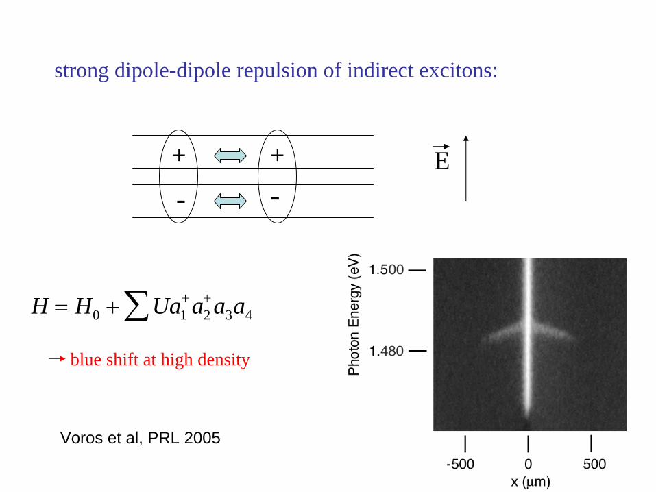
strong dipole-dipole repulsion of indirect excitons:

+ +

- -E

H = H0 + Ua1+a2

+a3a4∑blue shift at high density

Voros et al, PRL 2005

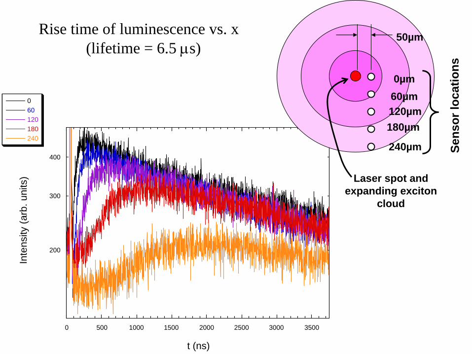
Rise time of luminescence vs. x(lifetime = 6.5 μs)

200

300

400

0 500 1000 1500 2000 2500 3000 3500

060120180240

Inte

nsity

(arb

. uni

ts)

t (ns)

Laser spot and expanding exciton

cloud

0µm

240µm

180µm120µm60µm

50µm

Sens

or lo

catio

ns

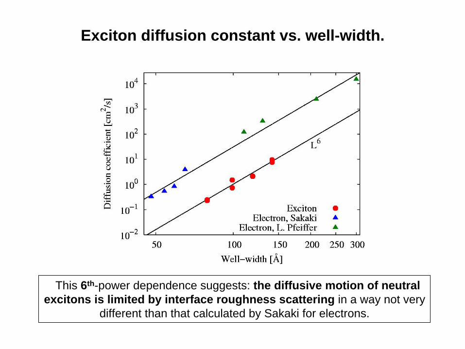
Exciton diffusion constant vs. well-width.

This 6th-power dependence suggests: the diffusive motion of neutral excitons is limited by interface roughness scattering in a way not very

different than that calculated by Sakaki for electrons.

T = 2 K

summary: tradeoff between binding energy and diffusion/disorder favorswider quantum wells (ca. 140 Å)

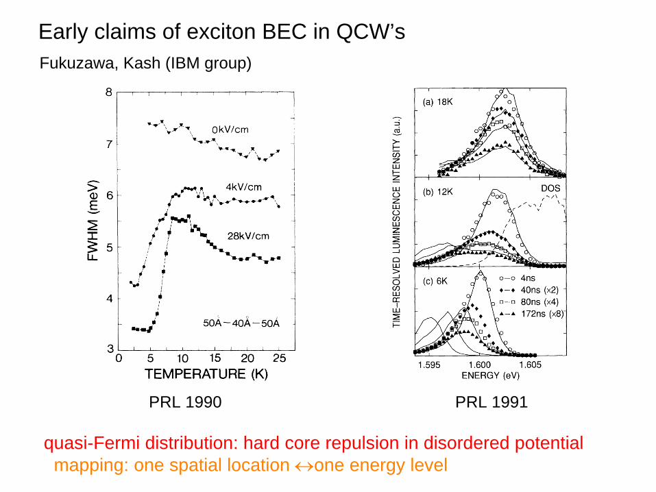
Fukuzawa, Kash (IBM group)

PRL 1990 PRL 1991

Early claims of exciton BEC in QCW’s

quasi-Fermi distribution: hard core repulsion in disordered potentialmapping: one spatial location ↔one energy level

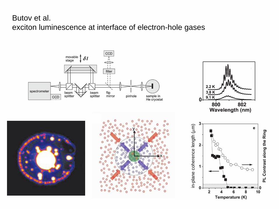
Butov et al.exciton luminescence at interface of electron-hole gases

in-p

lane

coh

eren

ce le

ngth

(μm

)

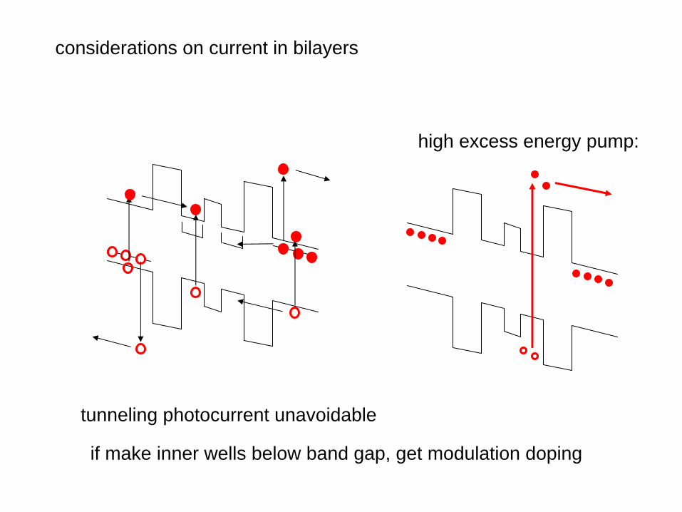
considerations on current in bilayers

tunneling photocurrent unavoidable

if make inner wells below band gap, get modulation doping

high excess energy pump:

Butov et al.exciton luminescence at interface of electron-hole gases

in-p

lane

coh

eren

ce le

ngth

(μm

)

hydrostatic strainshear strain

stra

in (a

rb. u

nits

)

x (mm)

-1.2 10 -4

-9 10 -5

-6 10 -5

-3 10 -5

0 10 0

3 10 -5

-1 -0.5 0 0.5 1

F

x

x

x

x

x

x

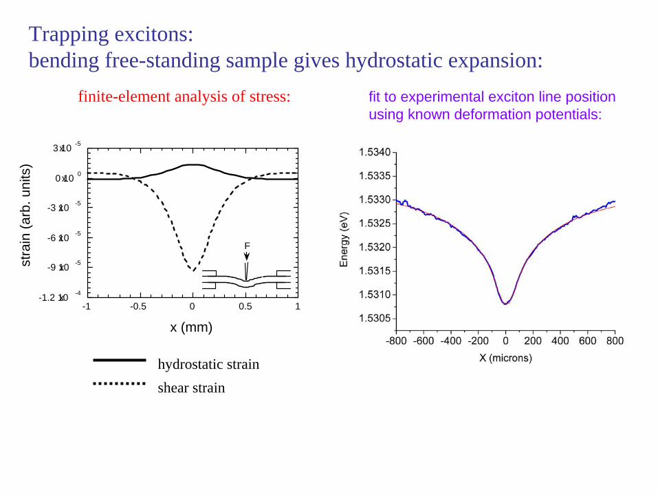
finite-element analysis of stress:

Trapping excitons:bending free-standing sample gives hydrostatic expansion:

fit to experimental exciton line position using known deformation potentials:

QuickTime™ and aVideo decompressor

are needed to see this picture.

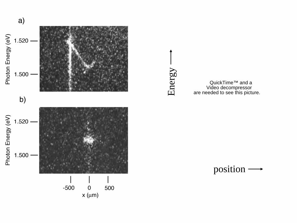
positionEn

ergy

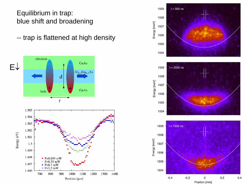
Equilibrium in trap:blue shift and broadening

-- trap is flattened at high density

E↓

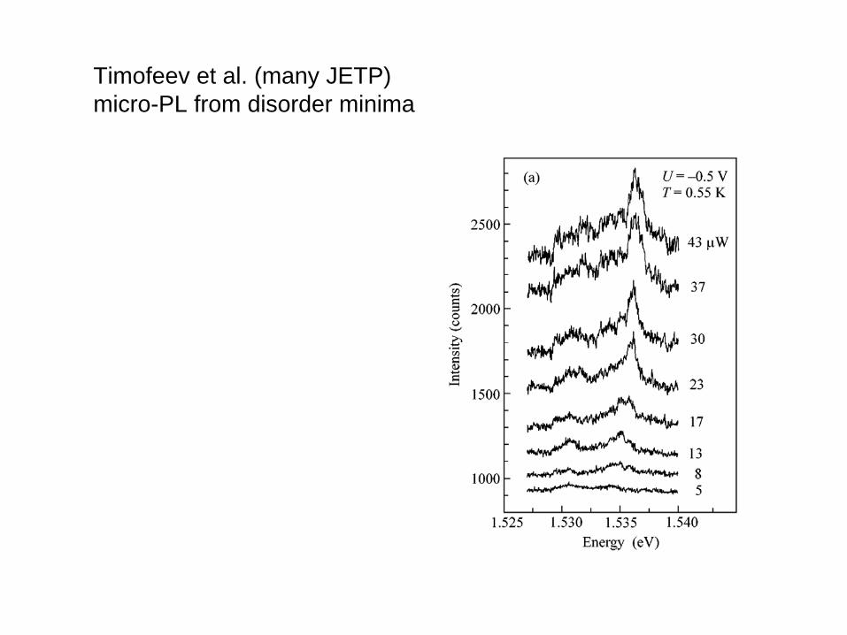
Timofeev et al. (many JETP)micro-PL from disorder minima

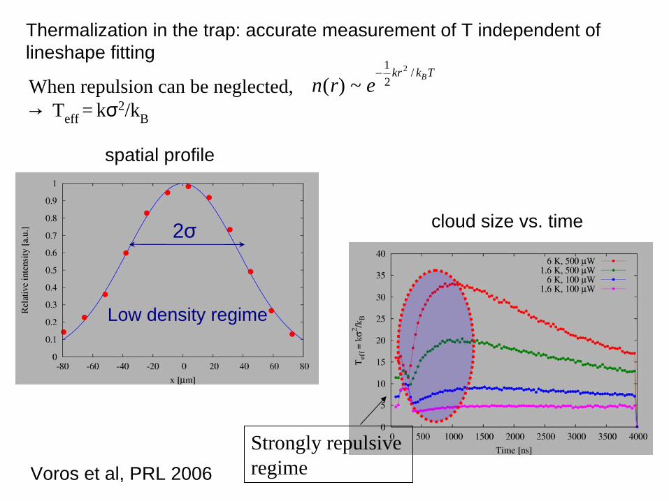
Strongly repulsive regime

When repulsion can be neglected, →

Teff = kσ2/kB

2σ

Low density regime

Thermalization in the trap: accurate measurement of T independent oflineshape fitting

Voros et al, PRL 2006

n(r) ~ e−

12

kr 2 / kBT

cloud size vs. time

spatial profile

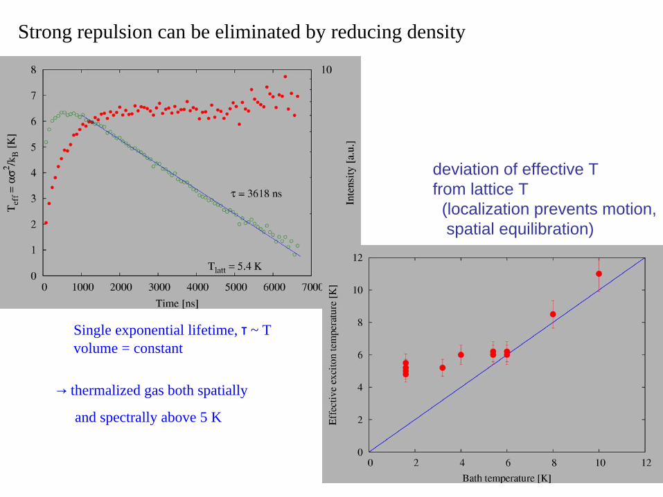
Strong repulsion can be eliminated by reducing density

Single exponential lifetime, τ

~ Tvolume = constant

deviation of effective Tfrom lattice T(localization prevents motion,spatial equilibration)

→

thermalized gas both spatially

and spectrally above 5 K

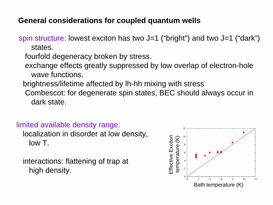
General considerations for coupled quantum wells

spin structure: lowest exciton has two J=1 (“bright”) and two J=1 (“dark”)states.

fourfold degeneracy broken by stress.exchange effects greatly suppressed by low overlap of electron-hole

wave functions.brightness/lifetime affected by lh-hh mixing with stressCombescot: for degenerate spin states, BEC should always occur in

dark state.

limited available density range: localization in disorder at low density,

low T.

interactions: flattening of trap athigh density.

Bath temperature (K)

Effe

ctiv

e E

xcito

nte

mpe

ratu

re (K

)

interactions: generally a difficult problem for all types of excitons.e-e exchangeh-h exchangee-h exchange

Like Ps, but gap is only ~100X greater than binding energy.Not a generally solved problem after 50 years!

Correlations play a huge role. mean-field theory differs fromexperiment by over an order of magnitude.

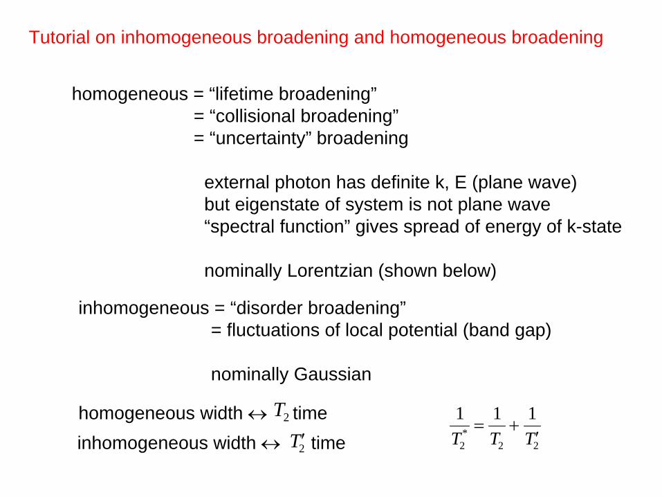
Tutorial on inhomogeneous broadening and homogeneous broadening

homogeneous = “lifetime broadening”= “collisional broadening”= “uncertainty” broadening

external photon has definite k, E (plane wave)but eigenstate of system is not plane wave“spectral function” gives spread of energy of k-state

nominally Lorentzian (shown below)

inhomogeneous = “disorder broadening”= fluctuations of local potential (band gap)

nominally Gaussian

1T2

* =1T2

+1′ T 2inhomogeneous width ↔

time′ T 2

homogeneous width ↔

timeT2

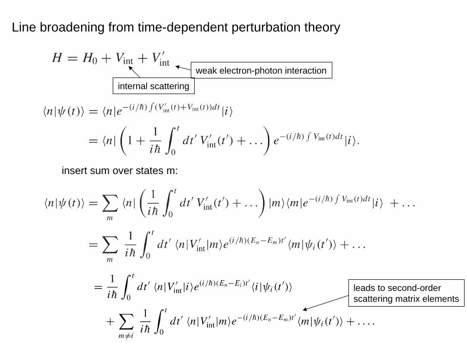
Line broadening from time-dependent perturbation theory

weak electron-photon interaction

internal scattering

leads to second-orderscattering matrix elements

insert sum over states m:

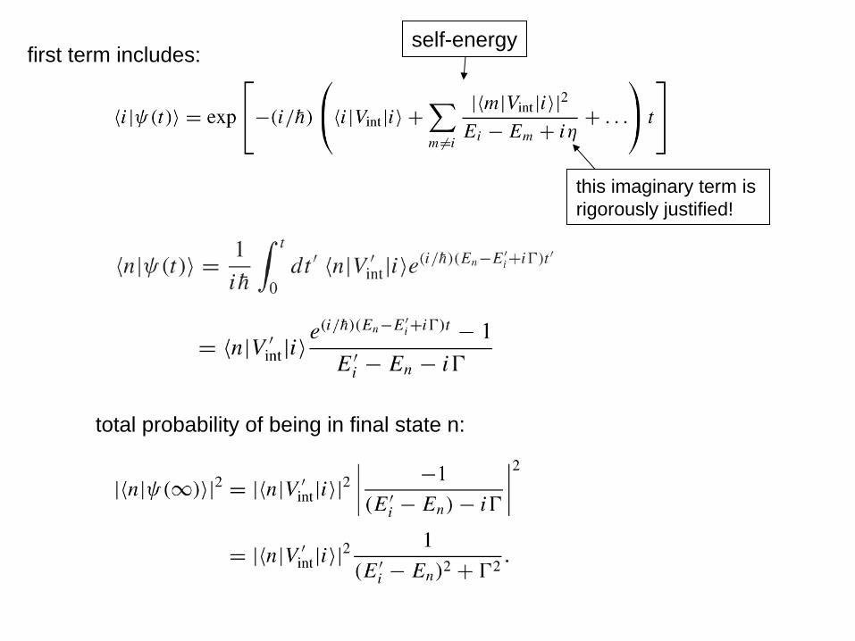
first term includes:

this imaginary term is rigorously justified!

total probability of being in final state n:

self-energy

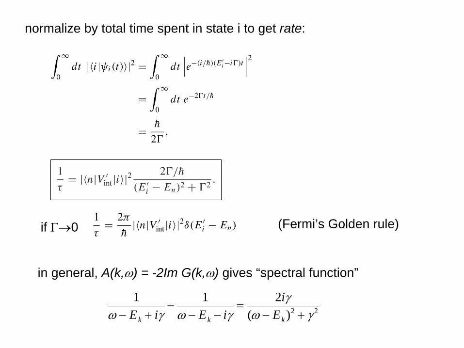
normalize by total time spent in state i to get rate:

if Γ→0 (Fermi’s Golden rule)

in general, A(k,ω) = -2Im G(k,ω) gives “spectral function”

1ω − Ek + iγ

−1

ω − Ek − iγ=

2iγ(ω − Ek )2 + γ 2

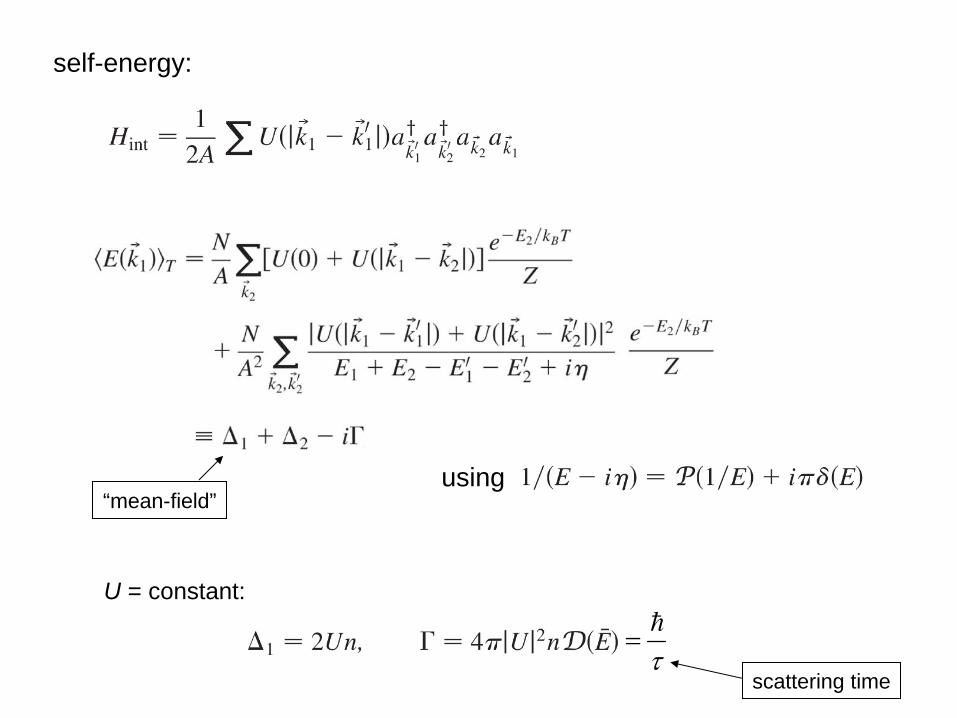
U = constant:

using

self-energy:

“mean-field”

=

h

τscattering time

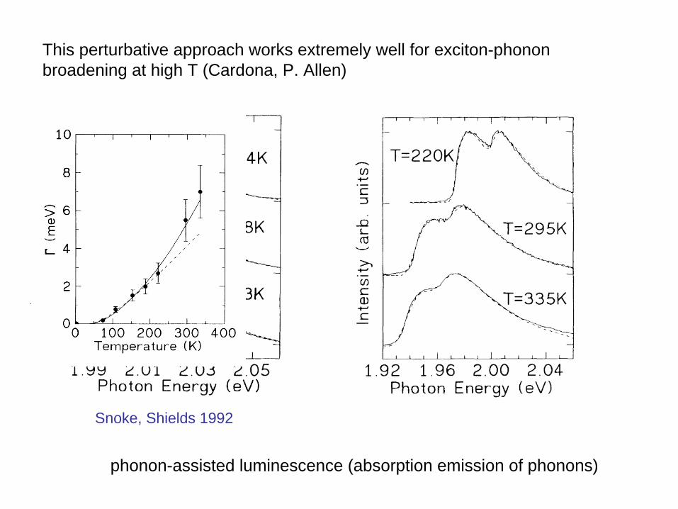
This perturbative approach works extremely well for exciton-phononbroadening at high T (Cardona, P. Allen)

phonon-assisted luminescence (absorption emission of phonons)

Snoke, Shields 1992

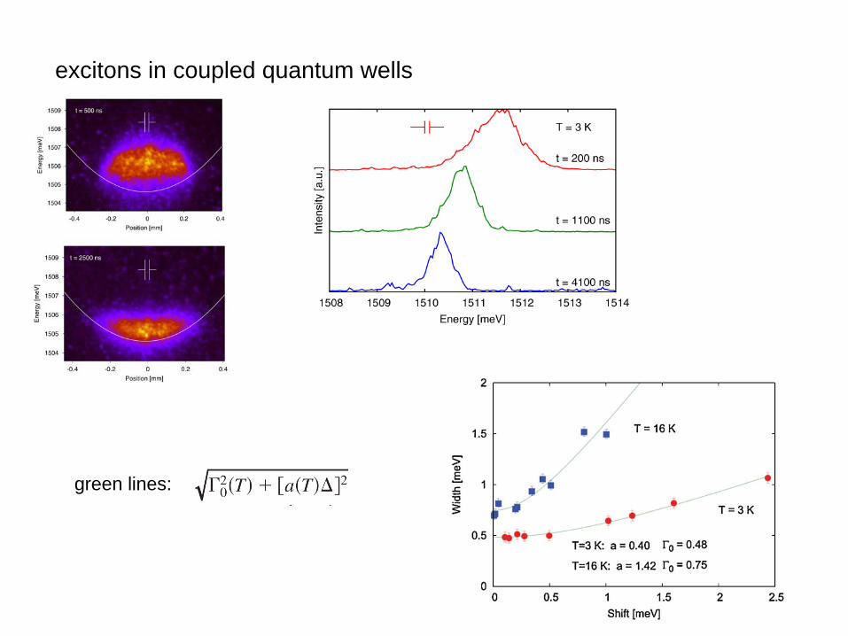
excitons in coupled quantum wells

green lines:

ratio

of w

idth

to s

hift

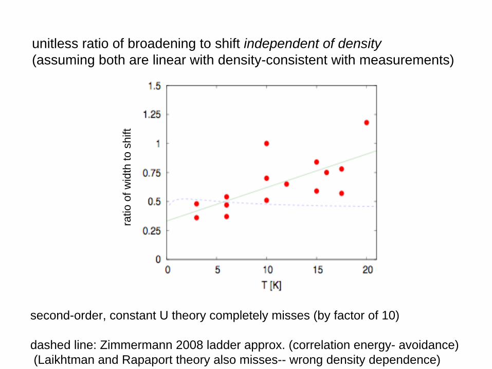
unitless ratio of broadening to shift independent of density(assuming both are linear with density-consistent with measurements)

second-order, constant U theory completely misses (by factor of 10)

dashed line: Zimmermann 2008 ladder approx. (correlation energy- avoidance)(Laikhtman and Rapaport theory also misses-- wrong density dependence)

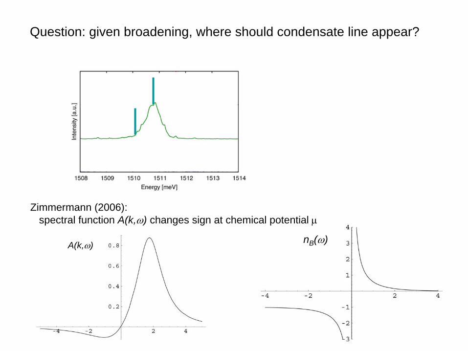
Question: given broadening, where should condensate line appear?

A(k,ω) nB (ω)

Zimmermann (2006):spectral function A(k,ω) changes sign at chemical potential μ

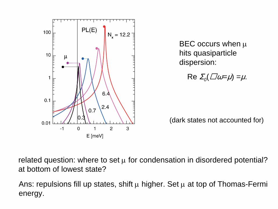
related question: where to set μ

for condensation in disordered potential? at bottom of lowest state?

BEC occurs when μhits quasiparticledispersion:

Re Σ0 ( ω=μ) =μ.

Ans: repulsions fill up states, shift μ

higher. Set μ

at top of Thomas-Fermienergy.

(dark states not accounted for)

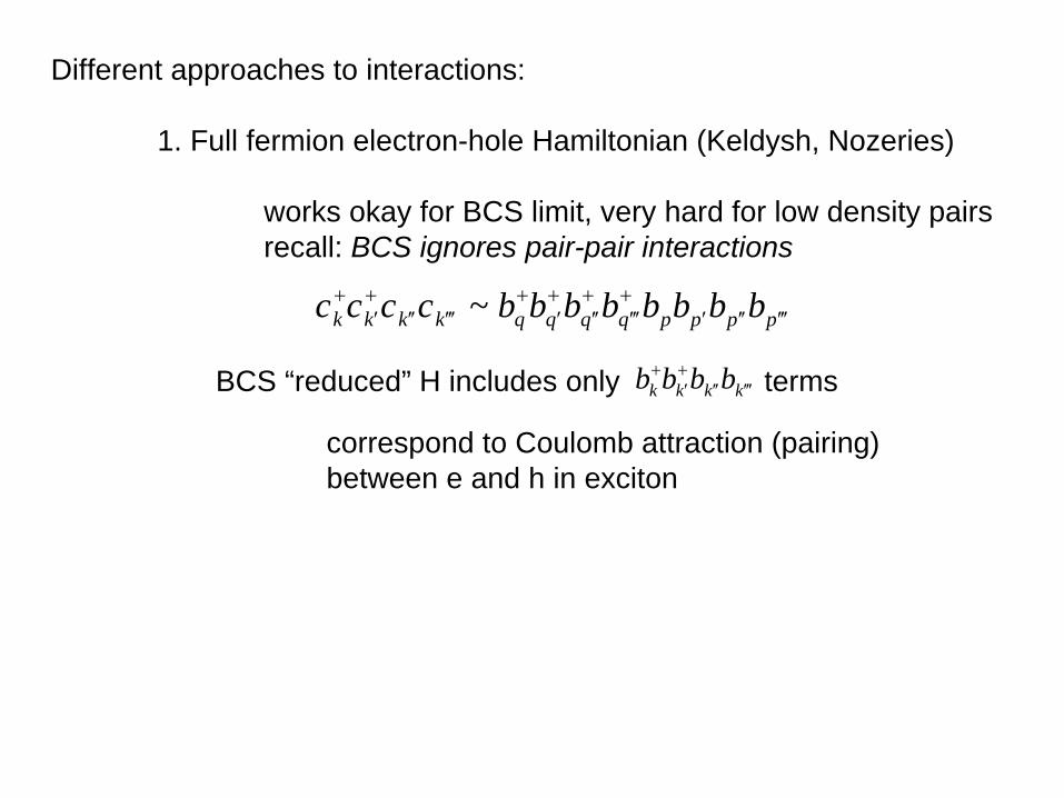
Different approaches to interactions:

1. Full fermion electron-hole Hamiltonian (Keldysh, Nozeries)

works okay for BCS limit, very hard for low density pairsrecall: BCS ignores pair-pair interactions

BCS “reduced” H includes only terms bk+b ′ k

+b ′ ′ k b ′ ′ ′ k

correspond to Coulomb attraction (pairing)between e and h in exciton

ck+c ′ k

+c ′ ′ k c ′ ′ ′ k ~ bq+b ′ q

+ b ′ ′ q + b ′ ′ ′ q

+ bpb ′ p b ′ ′ p b ′ ′ ′ p

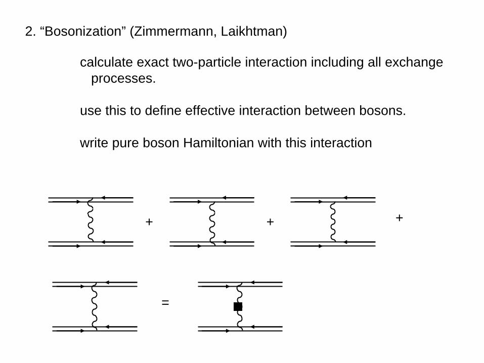
2. “Bosonization” (Zimmermann, Laikhtman)

calculate exact two-particle interaction including all exchangeprocesses.

use this to define effective interaction between bosons.

write pure boson Hamiltonian with this interaction

+ + +

=

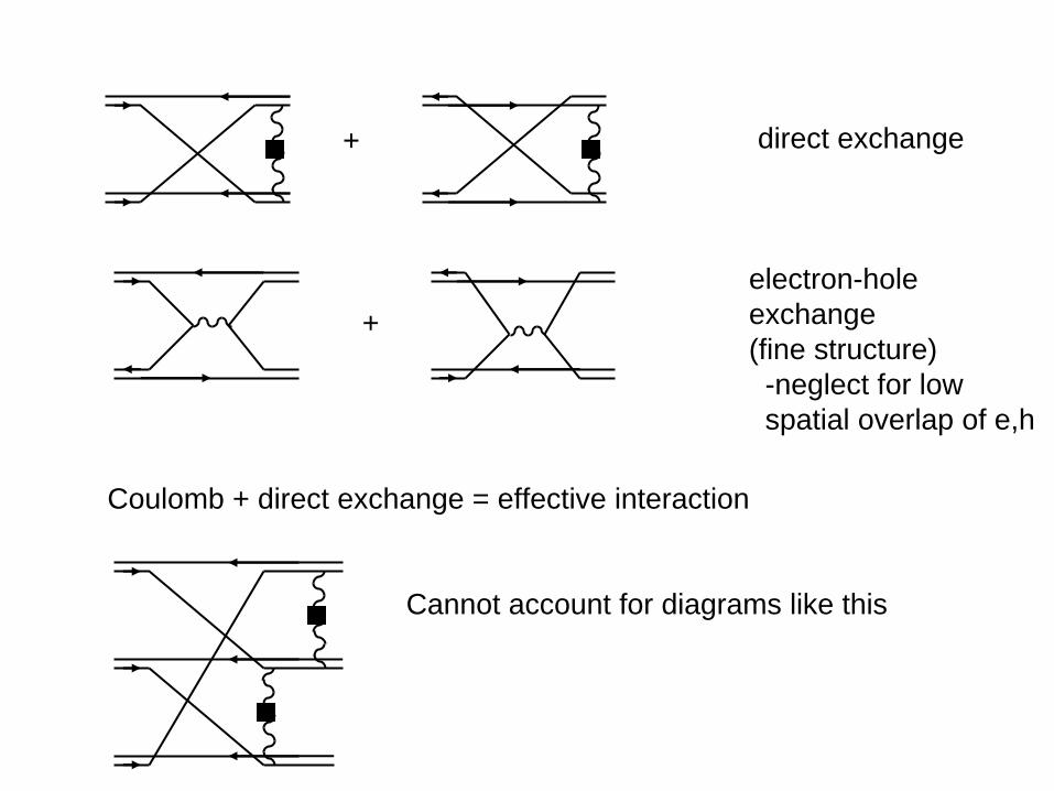
+ direct exchange

electron-holeexchange(fine structure)-neglect for lowspatial overlap of e,h

+

Coulomb + direct exchange = effective interaction

Cannot account for diagrams like this

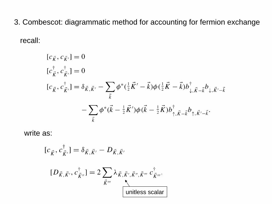
3. Combescot: diagrammatic method for accounting for fermion exchange

recall:

write as:

unitless scalar

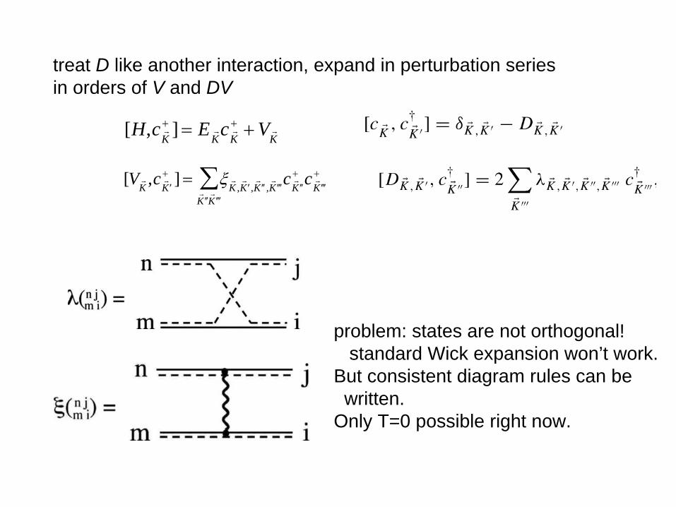
treat D like another interaction, expand in perturbation seriesin orders of V and DV

[H,c r K + ] = E r

K c r

K + + V r

K

[V r

K ,c r

′ K + ] = ξ r

K ,r

′ K ,r

′ ′ K ,r

′ ′ ′ K r ′ ′ K r

′ ′ ′ K

∑ c r ′ ′ K

+ c r ′ ′ ′ K

+

problem: states are not orthogonal! standard Wick expansion won’t work.

But consistent diagram rules can bewritten.

Only T=0 possible right now.

Not a unique problem of excitons! relevant whenever wavefunctionoverlap of fermions, which is always the case when condensation occurs.

Methods (2) and (3) both use unaltered exciton pair wave function φ(k).

In principle, should use variational adjustment of wave function φ(k) as density increases.

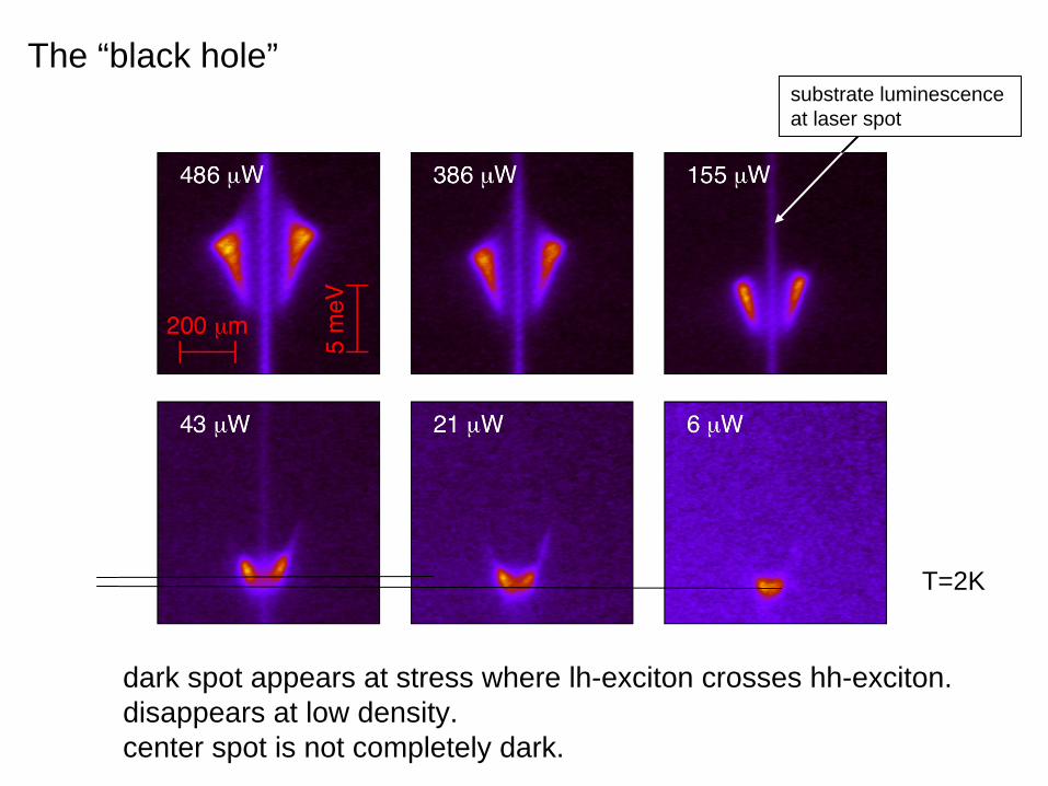
T=2K

The “black hole”substrate luminescence at laser spot

dark spot appears at stress where lh-exciton crosses hh-exciton.disappears at low density.center spot is not completely dark.

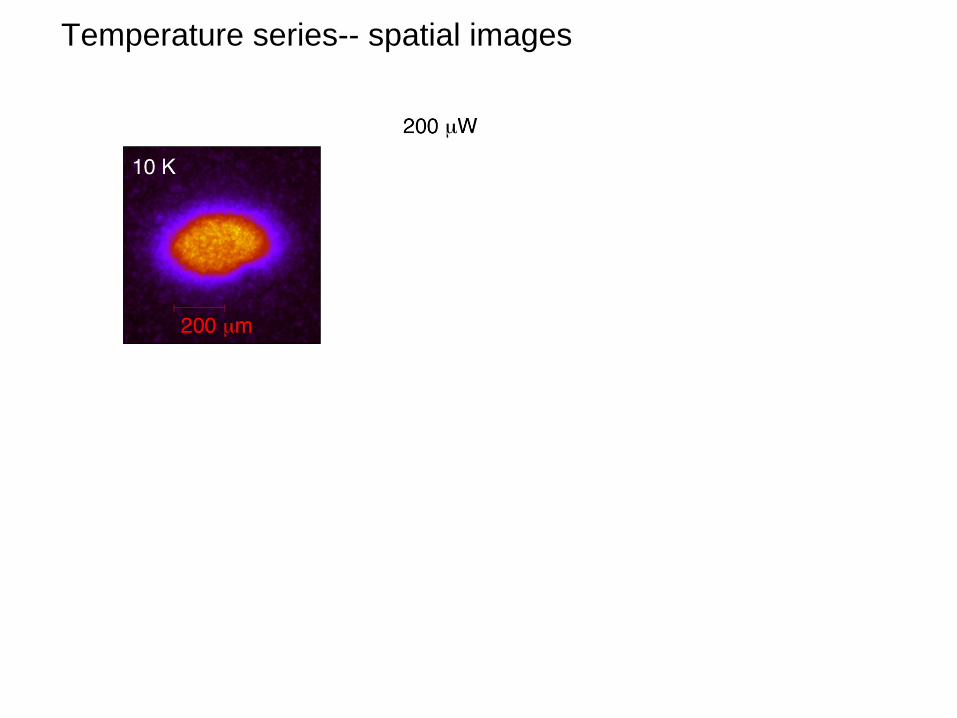
Temperature series-- spatial images

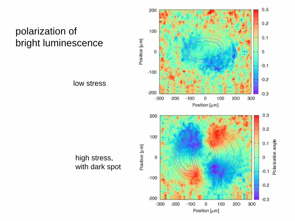
polarization of bright luminescence

low stress

high stress,with dark spot