Executive Market Segmentation: How Local DensityAffects Incentive and Performance

Hong Zhao∗,∗∗

W.P. Carey School of Business

Arizona State University

First Draft: December 2014

Current Draft: November 2015

*Department of Finance, W.P. Carey School of Business; hzhao25@asu.edu.** I am grateful to Ilona Babenko, Hank Bessembinder, Michael Hertzel, Laura Lindsey, Patrick McColgan,

Luke Stein, Ran Tao, Rong Wang, and seminar participants at Arizona State University, the 2015 China InternationalConference in Finance, the 2015 FMA Annual Meeting for helpful comments and discussion. All errors are my own.

Executive Market Segmentation: How Local DensityAffects Incentive and Performance

Abstract

This paper studies how the density of executive labor markets affects managerial incen-

tives and firm performance. I show that executive markets are locally segmented rather

than nationally integrated, and the density of a local market provides executives with non-

compensation incentives. In a denser market, executives face stronger performance-based

dismissal threats as well as better outside promotion opportunities. These incentives induce

executives to bring higher performance to firms in denser markets, especially when execu-

tives are young. The results in this paper imply the importance of local market density in

managerial incentive alignment.

JEL Classification: G30; G34; J42Keywords : Executive labor market; geographic segmentation; local market density; manage-rial incentive; firm performance

1 Introduction

Dismissal threats and promotion opportunities are important source of managerial incen-

tives. Jensen and Murphy (1990) show that dismissal threats account for 10% of a CEO’s

incentives, and Yermack (2004) finds that additional directorships account for 40% of an out-

side director’s incentives.1 Moreover, both theoretical and empirical research demonstrates

that these non-compensation incentives have positive effects on firm performance. For ex-

ample, Lazear and Rosen (1981) prove that an executive’s effort increases with the size of

promotion-based tournament incentive. Kale et al. (2009) and Coles et al. (2013) provide sup-

portive empirical evidence by documenting a positive relationship between firm performance

and intra-firm and intra-industry promotion opportunities, respectively.

This paper studies market density as one important determinant of both dismissal threats

and promotion opportunities. On one hand, executives in a denser area might face stronger

dismissal and promotion incentives because of peer competition and outside promotion op-

portunities. On the other hand, market density might disincentivize executives by providing

more backup options in the event of dismissals. Therefore, the goal of this paper is to examine

how local labor market density affects managerial incentives and what are the implications

on firm performance.

For local market density to matter, one necessary condition is geographic segmentation

in executive labor markets.2 If executives tend to move within one large national market

instead of many small local markets, then all executives will face the same competition

and promotion opportunities. To examine whether the U.S. executive labor markets are

geographically segmented, I explore the employment history of board directors and executives

covered by the BoardEx database. Using the zip code of firm headquarters, I calculate the

moving distance between the old and the new employers every time an individual changes a

1Applying more relaxed assumptions, Jenter and Lewellen (2014) show that CEO dismissal threats are substan-tially underestimated in previous literature.

2The U.S. executive labor markets are commonly viewed as very mobile. Kedia and Rajgopal (2009) write that“it is difficult to argue that top executives are geographically immobile” (p. 125). Yet, some recent empirical findingschallenge this view. For example, Yonker (2014) shows that firms are prone to hire CEOs who grew up in the state offirm headquarters than CEOs from elsewhere. Ang et al. (2013), Bouwman (2013), and Francis et al. (forthcoming)find that local geographic conditions could have substantial impacts on both the level and the structure of executivecompensation.

1

job. Out of 19, 692 job relocations in my sample, 6, 713 cases have a moving distance of 60

miles or less (i.e. local). To conduct formal tests on segmentation, I compare the realized

local hiring percentage with the expected local hiring percentage under the null hypothesis

that the executive market is nationally integrated. For each hiring event, the expected local

hiring probability is approximated by the number of local firms divided by the number of

firms nationwide. I find that the expected local hiring percentage is around 5%, while the

realized percentage is 34%. This implies that local hiring bias is 29%, or firms hire local

executives seven times more often than expected. A binomial test indicates that this bias is

statistically significant. One concern with the above local hiring bias is that it might actually

be driven by geographic clustering of industry and firm’s tendency of hiring industry insiders.

To disentangle industry effect from the bias, I adjusted the expected local hiring probability

based on number of firms within the same industry as the hiring firm. With this alternative

measure, LHB is still significantly above zero at 25%.

Based on the evidence of geographic segmentation, I then study how local labor market

density affects executive’s implicit incentives through dismissal threats and outside promo-

tion opportunities.3 Since firms often hire executives from the local pool, firms located in

denser markets face more outside candidates and lower replacement cost. Therefore, local

density makes firms more likely to dismiss poor-performing executives, and hence creates a

performance-induced dismissal threat for executives. Besides dismissal threats, local density

could also improve executive incentive alignment through the channel of tournament incen-

tives. To the extent that executives in a denser market have more potential outside positions

to be promoted to, both the prize of the tournament and the probability of winning might

increase with market density.

To provide empirical evidence that density of the local market creates implicit incen-

tives for executives, I first examine the relation between market density and CEO turnover-

performance sensitivity. I measure density as the number of firms within 60 miles of a firm

headquarters. Using CEO turnovers during 1996 − 2013, I find that the sensitivity of CEO

turnover to stock performance rises as the density of local executive pool rises. Such effect3In this paper, I call managerial incentives from dismissals and tournaments implicit incentives to distinguish

them from explicit incentives generated by compensation structures.

2

is both statistically and economically significant. An interquartile increase in density raises

the turnover-performance sensitivity by 20%. I also find that outside successions are more

frequently used by firms in denser markets. These results are consistent with my hypothesis

that convenient access to outside candidates in denser labor markets leads to firms dismissing

poor-performing incumbent executives more frequently.

Next, I investigate whether denser markets also create stronger outside promotion incen-

tives for local executives. Similar to Kale et al. (2009) and Coles et al. (2013), I consider

both the tournament prize and the probability of winning. I measure tournament prize as

the compensation gap between executive’s current compensation and the 90th percentile of

compensation in the local market, and measure winning probability as the realized executive

promotion frequency. Empirically, both compensation gap and outside promotion probability

are higher in denser labor markets. The effect of local market density are statistically sig-

nificant and large in magnitude. For executives changing jobs between Execucomp firms, an

interquartile increase in market density raises expected tournament prize from $0.86 million

to $3.1 million, and raises local outside promotion frequency by about 60%.

Although local market density provides executives with implicit incentives through dis-

missal threats and outside promotion opportunities, it is also possible that density could

disincentivize executives by offering more backup options in the event of a dismissal. To

test such argument, I construct a sample of executives losing their jobs and examine their

subsequent employment outcomes. Applying a similar procedure to Fee and Hadlock (2004),

I consider all executives in S&P 500 firms who were under the age of 55 and lost jobs dur-

ing 2000 − 2010, and look for their subsequent employment history in a three-year window

based on news articles. Regression results indicate that local market density does not help

dismissed executives find a new job more easily, obtain a higher-quality position, or experi-

ence shorter unemployment duration. One reason for local market density having no effect

on post-dismissal employment outcome is that potential local employers could have detailed

information on those poor-performing executives and are thus reluctant to hire them. I find

empirical evidence supporting this explanation. The probability of firms hiring a local dis-

missed executive is only half the probability of firm hiring a local non-dismissed executive,

3

suggesting that executive reputation spreads in local labor markets.

Since local market density generates strong implicit incentives for executives, the last

goal of the paper is to examine whether density enhances firm performance through incentive

alignment. The empirical challenge here is that market density could have an impact on

performance through various channels, so a simple positive correlation between these two

variables does not suffice.4 To distinguish the incentive mechanism from other potential

mechanisms, I interact market density with executive’s career horizon. The logic, as argued

in Gibbons and Murphy (1992), is that executives with a shorter horizon (closer to retirement)

should respond less to dismissal and promotion incentives. Using executive’s current age as

a proxy of horizon, I find that the coefficient on the interaction term between market density

and executive horizon is significantly positive in performance regressions. In other words,

the positive effect of market density on firm performance is stronger for firms with younger

executives. As for economic magnitude, firms in markets at top-quartile density and with

executives at bottom-quartile age have a 0.35 (0.01) higher Tobin’s Q (ROA) than firms in

markets at bottom-quartile density and with executives at top-quartile age. These results are

consistent with my argument that executives in a denser market exert more effort in response

to stronger implicit incentives and thus improve firm value.

I use the number of local firms as the main measure of local labor market density, but I

also consider several alternative measures. Since larger firms provide more job positions and

more executives than small firms do, I adjust each count of firms in a local market by firm’s

employment size. Also, if executives often change jobs within rather than across industries,

a more appropriate measure of local density would include only local firms which are in the

same industry as the target firm. Using these alternative measures, I find that the findings

on managerial incentives and firm performance remain unchanged.

It is likely the case that the geographic segmentation documented in this paper is driven by

firm’s and executive’s endogenous choices rather than natural barriers. Firms might choose

to hire local executives because information asymmetry is less severe in local markets, or it

takes less effort to hire those nearby. Executives might choose to relocate locally because the4See Marshall (1920), Duranton and Puga (2004), and Rosenthal and Strange (2004) for economic foundations on

the effects of geographic clustering on firms.

4

physical or emotional moving costs are large. However, to the degree that local density affects

incentives as long as firms knows that they are likely to find successors locally and executives

know that are likely to obtain their next job locally, the reason that causes segmentation,

either endogenous or exogenous, does not matter.

The empirical findings suggest that executives in denser markets face stronger incentives

and achieve better performance through the channel of local competition and promotions.

Yet, density might also be associated with other firm or market characteristics, such as

board independence, that have a direct impact on incentives and performance (Knyazeva

et al. (2013)). For results on incentives, endogeneity is less of a problem. Even if board

independence affects dismissal threats and promotion opportunities, it does not contradict the

findings that density enhances incentive alignment. It merely suggests that higher incentives

in denser markets might also be created by board independence, in addition to competition

and promotions as argued in this paper. Endogeneity could be more of an issue for results

on firm performance, where I intend to specify the channel through which density affects

performance. To demonstrate the incentive alignment channel, I explore the heterogeneity of

the density effect with respect to career horizon. I also control for the board independence

channel and find that the main results are not attenuated.

This paper contributes to several streams of research in the finance literature. First,

by examining whether the U.S. executive labor market is geographically segmented, it con-

tributes to the burgeoning literature on executive market geography. Several recent studies

(e.g. Francis et al. (forthcoming), Ang et al. (2013), and Bouwman (2013)) implicitly as-

sume the existence of segmentation in executive markets and find geographic patterns in

executive compensation structures. Yet, none of them provides a direct test on the segmen-

tation assumption. To this extent, my paper fills the gap in the literature by documenting

a strong bias of firms hiring and executives moving locally. Second, my study relates to the

literature on executive incentives. Besides explicit incentives from compensation contracts,

another source of incentive alignment comes from implicit incentives, including rank-order

tournaments (Lazear and Rosen (1981), Green and Stokey (1983), Kale et al. (2009), Coles

et al. (2013)) and performance-induced dismissal threats (Jenter and Lewellen (2014)). My

5

results indicate that local market density creates both tournament incentives and dismissal

threats, and executives respond to these implicit incentives based on their level of career hori-

zon. Finally, my paper extends the literature studying the effect of geographic agglomeration

on firms. Existing work finds that geographic agglomeration affects firms in many aspects,

including innovation (Glaeser et al. (1992)), acquisition (Almazan et al. (2010)), dividend

policies (John et al. (2011)), and board independence (Knyazeva et al. (2013)). Focusing on

executive labor markets, I find that firms located in denser areas are more likely to dismiss

poor-performing executives and hire outsiders. Moreover, local density enhances firm value

through the channel of executive incentives. My study on executive markets provides an

alternative way to interpret the impacts of geographic agglomeration on firm performance.

The rest of the paper is organized as follows. Section 2 provides a review of related lit-

erature. Section 3 examines geographic segmentation in the U.S. executive labor market.

Main results on managerial incentives and firm performance are provided in Sections 4 and

5. Section 4 studies how local labor market density affects dismissal threats and outside pro-

motion opportunities for executives. Section 5 investigates whether market density improves

firm performance through the channel of incentive alignment. Section 6 conducts robustness

checks and explores alternative explanations. Section 7 concludes.

2 Related Literature

2.1 Executive Market Geography

If firms search executive candidates in a nationwide pool and executives are highly mobile,

geographic conditions should have no impact on executive compensation, incentive, and etc.

Yet, this view of an integrated executive market is not supported by recent empirical studies.

Comparing firms in urban and rural areas, Francis et al. (forthcoming) find a positive

relation between a firm’s headquarters metropolitan size and the total and equity portion

of its CEO’s pay. They further show that firms in dense areas are willing to offer this

compensation premium because agglomeration improves executive local network and human

capital accumulation. Ang et al. (2013) find a similar positive relation between local market

density and CEO compensation. They refer to sociology literature and explain this positive

6

relation as a result of CEO social comparison and social pressure from local peers. Also

based on sociology literature, Bouwman (2013) documents that CEO compensation level

highly depends on the average level of local peers. She tests several explanations for this

phenomenon and concludes that it is most consistent with CEO envy. To the degree that

executive compensation has geographic patterns and firm location is largely exogenous to

current executives, local geographic conditions could be exploited as instrumental variables

in the study on executives. For instance, Coles et al. (2013) use average local compensation

as an instrument to CEO compensation and study the effect of industry tournament incentive

on firm performance.

The study most directly testing on geographic segmentation of executive labor market is

Yonker (2014), who finds that firms are five times more likely to hire CEOs who grew up in the

same state as firms’ headquarters (home hiring bias). However, unlike local hiring bias, home

hiring bias is not direct evidence on geographic segmentation because executive’s hometown

could be different from the location of his previous job.5 Also, Yonker measures geographic

proximity at state level and uses a sample consisting of only 1, 162 CEO hirings. These

restrictions preclude more detailed and comprehensive conclusions on the overall executive

labor market. Using executive job changes covered in BoardEx and calculating zip code

distance between executive’s old and new firms, my paper addresses these issues.

2.2 Managerial Incentives

Managerial incentive has been the core of studies on corporate governance. Hölmstrom

(1979) builds the foundation of modern principal-agent model and derives the optimal man-

agerial contract under imperfect information and moral hazard. Following this theoretical

work, hundreds of researchers have been investigating the empirical relation between firm

performance and executive compensation structures. Important early contributions include

Morck et al. (1988) and McConnell and Servaes (1990), who find non-linear and “hump-

shaped” relation between firm Tobin’s Q and executive ownership. Yet, numerous later

5Suppose a CEO spent his childhood in California, worked as a senior executive in a New York firm, and thenwas hired by a Californian firm as CEO. In such case, it is clear that the Californian firm has conducted a nationwidesearch and the CEO moves across the nation, but the hiring would be classified as a local one if CEO’s “grew-up”area rather than CEO’s last job area is used.

7

studies using different data and methods yield conflicting results.6 More recently, Coles et al.

(2012) use structural estimation to address the issue of endogeneity and conclude that the

“hump-shaped” relation between firm value and executive ownership is an equilibrium result

driven by exogenous firm characteristics.

Apart from compensation, internal and external labor market outcomes provide execu-

tives with another source of incentives. This paper focuses on executive external tournament

incentives and internal dismissal threats. Theoretical foundations of rank-order tournament

are developed by Lazear and Rosen (1981) and Green and Stokey (1983). They show that

tournaments can replace performance-based contracts as an incentive mechanism and that

tournaments can lead to more efficiency under some circumstances. On the empirical side,

Kale et al. (2009) measure non-CEO executive’s internal tournament incentives using the pay

gap between the non-CEO executive and CEO within the firm. They find that tournament

incentives have a positive effect on firm performance after controlling compensation incen-

tives and addressing endogeneity. They also show that such positive effect is stronger when

executive’s perceived promotion probability is higher. Coles et al. (2013) extend Kale et al.

(2009) by examining tournament incentives on CEOs. They argue that, although CEOs have

no promotion incentives within the firm, they are still in a tournament with CEOs outside the

firm. They use the compensation gap within industry as a measure of tournament incentives

and find a positive relation between industry tournament incentives and firm performance.

Similar to Kale et al. (2009), they find that tournament incentives are stronger when CEOs

perceive higher probability of being promoted. Fee and Hadlock (2003) also confirm the

existence of promotion incentives by showing that executives who jump to CEO positions at

new employers come from firms with superior stock performance. Like promotions, dismissals

also generate incentives for executives. Previous studies document a robust negative relation

between firm stock performance and executive turnover probability, though the magnitude is

modest.7 Using more relaxed model assumptions such as non-linearity, Jenter and Lewellen

(2014) uncover a much larger effect of firm performance on CEO turnover than previous6Demsetz and Villalonga (2001) provide a review and discussion on the empirical relation between ownership and

performance.7See, among others, Coughlan and Schmidt (1985), Warner et al. (1988), Weisbach (1988), Denis et al. (1997),

Huson et al. (2001), and Kaplan and Minton (2012).

8

studies and thus argue that performance-induced dismissal threat is an essential source of

incentives. One feature of labor market incentives, both dismissals and promotions, are that

their strength depends on executive career horizon. Promotions become less attractive and

dismissals become less threatening when executives are closer to retirement, i.e. shorter career

horizon. Gibbons and Murphy (1992) show both theoretically and empirically that horizon

affects labor market incentives and firms optimally adjust the level of explicit incentives in

compensation contracts based on the strength of career concerns.

2.3 The Effect of Geographic Clustering on Firm

Firm location choices and geographic clustering have been discussed by economists since

Marshall (1920). Marshall theorizes three primary benefits to firms locating in clusters:

knowledge spillovers, labor market pooling, and input providers pooling. Although the em-

pirical evidence on the direct impact of clustering on performance is mixed, economists do

find that these three channels exist. For example, using patent citation as a “paper trail” of

knowledge flow, Jaffe et al. (1993) find that knowledge spillovers attenuate with geographic

distance since citations are highly spatially concentrated. Glaeser et al. (1992) also finds

evidence on knowledge spillovers using data on industry growth. Evidence on labor market

pooling and input providers pooling are documented in Costa and Kahn (2000) and Holmes

(1999). On the other hand, geographic clustering could also have negative effects on firms.

Shaver and Flyer (2000) argue that the strongest firms gain little from clustering, yet suffer

when their technologies and employees spillover to competitors. Other costs of agglomeration

include transportation congestion, pollution, and crime (Glaeser (1998) and Tabuchi (1998)).

Duranton and Puga (2004) and Rosenthal and Strange (2004) provide comprehensive reviews

of both theoretical foundations and empirical results of the literature.

Besides these economic foundations, geographic agglomeration could also affect firms

through reasons well-established in the finance literature. For example, Almazan et al. (2010)

find that firms located in clusters have more acquisition opportunities. They also show that

these firms maintain more financial slack than their industry peers in order to facilitate po-

tential acquisitions. One reason for firms in clusters having more acquisition opportunities,

9

as argued in Uysal et al. (2008), is that geographic proximity leads to information advantage.

They find that acquirer returns are significantly higher in local acquisitions than in non-local

ones. Market density could also influence firm dividend policy. Based on agency theory, John

et al. (2011) show that firms located far away from large metropolitan areas use precommited

high dividends as a solution to the potential agency problem due to decreased shareholder

monitoring ability. The study most closely related to my paper is Knyazeva et al. (2013).

They consider the size of clusters as a proxy of the thickness of outside directors pool. Em-

pirically, they show that firms located in denser markets have higher board independence

and better performance.

3 Geographic Segmentation in the U.S. Executive Labor Market

This section documents the geographic segmentation in the U.S. executive labor market.

To deliver robust results, I consider a set of different measures of expected local hiring per-

centage under the null hypothesis of a nationwide executive labor market. Further subsample

analyses are provided in Appendix B.

3.1 Executive Job Changes Sample

I explore individual employment histories covered by the BoardEx database of Manage-

ment Diagnostics Ltd. BoardEx provides comprehensive biographical information on indi-

viduals who have ever been listed as either directors or disclosed top earners in public traded

U.S. companies since 2000. Currently, the database covers about 71% of firms in Compustat,

representing 95% of market capitalization. At each report date, an individual’s curriculum

vitae is constructed based on the most recent publicly disclosed information. I explore the

professional working experience contained in the curriculum vitae.8

I order each individual’s employment history in a chronological order, and record a job

change if the his employer in year t is different from the employer in year t+1. Since BoardEx

reports job beginning and end dates in either year-month or year based on data availability,

I convert all dates into year format.9 I exclude about 25% job changes where there is a gap8Since the employment history of either directors or top earners mainly contains senior executive roles in various

companies, I call directors and top earners both executives when I refer to their employment history.9I drop employment observations with a missing start year or end year, unless it is an executive’s first employment

10

between the end year of the old job and the start year of the new job, because executives

could have a job and relocate during that gap while just not identified by BoardEx. I further

only keep job changes between U.S. public firms because location data on private firms are

not readily available. Since large firms benefit more from a nationwide job search and have

lower local hiring bias (as supported by the empirical evidence in Appendix B), the bias

documented here could be regarded as a lower-bound.

To calculate the moving distance between the old and new firms, I merge BoardEx with

Compustat by linking the International Security Identification Number (ISIN) from BoardEx

with the CUSIP from Compustat. For U.S. firms, the ISIN is constructed by adding “US” to

the front and a single-digit check code to the end of the regular nine-digit CUSIP number.

I then merge the zip code of firm’s headquarters from Compustat with the latitude and

longitude of each zip code from the Census 2000 U.S. Gazetteer.10 The distance in miles

between two zip code areas is calculated using the Vincenty formula.11

The main sample consists of 19, 692 executive job changes, with 16, 277 unique executives

and 3, 743 unique hiring firms. The sample mean (median) total assets of hiring firms are

9.75 (1.63) billion of 2000 U.S. dollars. Compared to the firms in the Compustat universe

during the similar time span with mean (median) assets of $5.59 ($0.16) billion, the hiring

firms in my sample mainly consists of the large U.S. firms.

3.2 Estimation Strategy

Following the literature (e.g. Knyazeva et al. (2013), Bouwman (2013)), I define a firm’s

local area as the area within a 60-mile radius of the firm’s headquarters. I use 100-mile and

250-mile radii as alternative cutoff values. Similar to Yonker (2014), I calculate local hiring

record for a missing start year or the last employment record for a missing end year. About one-third observationsare dropped.

10Compustat reports the current headquarters location of firms. Knyazeva et al. (2013) show that the overwhelmingmajority of firms do not relocate. Even for firms that relocate, most of them remain within sixty miles of their previouslocation. I also implicitly assume that all executives holding senior positions work at the firm’s headquarters.

11The Vincenty formula is often used in measuring distances in the finance literature (see Pool et al. (forthcoming)for example). It calculates the distance between two points on the surface of a spheroid. The distance in miles betweentwo zip code areas with latitude/longitude (ϕi, λi) is calculated as

3963.19× arctan(

√(cosϕ2sin(λ2 − λ1))2 + (cosϕ1sinϕ2 − sinϕ1cosϕ2cos(λ2 − λ1))2

sinϕ1sinϕ2 + cosϕ1cosϕ2cos(λ2 − λ1))

11

bias (LHB) as the difference between the realized local hiring percentage and the expected

local hiring percentage under the null hypothesis that the executive market is nationwide.

Formally,

LHB =NL

N−

∑Ni=1 piN

where N is the total number of hiring event in my sample, NL is the number of actual local

hiring, and pi is the probability of hiring a local executive for each hiring event i under the

null hypothesis.

To calculate LHB , I propose several methods to estimate the key element pi. The first

and the most straightforward measure is the number of local firms of event firm i divided

by the number of firms nationwide.12 However, this simple ratio measure does not take into

account that large firms might provide more executives to local labor market than small

firms. Thus, in the second measure I adjust the ratio using firm size. Specifically, each firm

count is adjusted by a size weight, which is calculated as the firm’s number of employees

divided by the average number of employees for all firms in that year.

One concern with LHB calculated using either of the two measures of pi is that the bias

might actually be driven by a firm’s tendency to hire industry expertise rather than locals.13

For example, consider Google in Silicon Valley. Suppose, at the extreme, that Google only

hire executives within the same industry. Since many of the high-technology firms are located

in Silicon Valley, one would expect to observe a high realized percentage of local hiring for

Google. To address this issue and separate industry effects from local effects, I calculate

a third measure of pi as the number of local firms within the same industry as the event

firm divided by number of firms of that industry nationwide. Industry is classified based on

2-digit SIC codes. Under this measure, if Google tends to hire industry veterans but not

locals, the expected local hiring percentage pi will be high for Google due to the industry

clustering effect and LHB should not be different from zero. Finally, the fourth measure of

pi adjusts the third measure by firm size as done for the second measure.

As for Google in 2010, the 60-mile expected local hiring percentages under p1 and p2

12Throughout the paper, I only consider firms that are covered by Compustat except otherwise noticed.13Based on my sample, 48.3% of job changes are within the same 2-digit SIC industry.

12

are 0.09 and 0.04, respectively. When industry clustering effects are taken into account, the

expected local hiring percentages under p3 and p4 increase to 0.16 and 0.12. To the extent

that firms hire executive both within and outside of the industry, LHB estimated using pi

from the first two (cross-industry) and last two measures (within-industry) could be regarded

as upper and lower bounds of the local hiring bias.

3.3 Results on Local Hiring Bias

Table 1 presents the results on local hiring bias based on the 19, 692 executive job changes

identified in Section 4.1. In Panel A, I conduct a baseline analysis for the full sample using p1

in the LHB calculation. The first and second columns list the total number of hiring events

N and the number of realized local hirings NL. The third column shows the realized local

hiring percentage, which is calculated as column (2) divided by column (1). The fourth and

fifth columns show the total number of expected local hiring and the expected local hiring

percentage under null hypothesis of a nationwide market. Finally, the last column calculates

the local hiring bias as the difference between column (3) and column (5).

As reported in Panel A, when a 60-mile is used, 34% of hirings are local. However, if the

executive labor market is integrated and nationwide, the expected local hiring percentage

should be around 5%. Therefore, the local hiring bias is 29%. In other words, firms hire

local executives seven times more often than they would if the market were integrated. In

the next two rows, I use 100-mile and 250-mile as alternative cutoffs to define the local

area. The magnitude of the local hiring bias remains substantial and is around 29% to 31%.

Another thing worth noticing is that although there are 6, 713 hirings within 60 miles, only

410 (1, 951) additional hirings happen between 60 and 100 miles (100 and 250 miles). The

number of these additional hirings are actually close to the increase in expected hirings.

Hence, it could be that the local hiring bias is mostly driven by the hirings within 60 miles of

the firm’s headquarters. In Panel B, I replace the unadjusted expected local hiring measure

p1 with size adjusted measure p2. As shown in the last column, the bias continues to exist

and becomes even larger.

To address the concern that local hiring bias could actually be driven by firm’s tendency

13

to hire industry insider, I use the third and fourth measure of pi in Panels C and D. Consistent

with the fact that firms within the same industry often cluster together, the expected local

hirings are almost double the numbers in Panels A and B. Although the increase in expected

local hirings reduces the bias, it is still substantially larger than zero for both unadjusted

and size adjusted pi measures and all three distance cutoffs. As argued in Section 4.2, since

the cross-industry and within-industry measures of pi provide an upper and lower bounds of

LHB , the results in Panels A and B together indicate that the local (60-mile) hiring bias is

between 25% to 29%, and firms are three to seven times more likely to hire local executives

than expected.

In addition to economic magnitude, I also compute statistical significance using a two-

sided binomial test where a local hiring is considered as a success. Formally, for the binomial

test, the number of trials is N , the number of successes is NL, and the probability of success

is the average of pi (∑N

i=1 pi/N). The test results reject the null hypothesis that the executive

labor market is integrated for all distance and pi measures in Panels A and B at the 1% level.

4 Local Market Density and Executive Incentive Alignment

In Section 3, I document the phenomenon that there exists a substantial geographic

segmentation in the U.S. executive labor market. If firms often hire and executives often

move locally, then the density of the local labor market could have an impact on executive

incentives. In this section, I first provide empirical evidence on how labor market density

affects executive’s dismissal threats, as measured by turnover-performance sensitivity. Then,

I show that executives in denser area have better outside promotion opportunities, in terms

of larger compensation gap as well as higher promotion probability. Finally, by studying the

subsequent employment outcomes for executives who lose their jobs, I address the concern

that the market density might disincentivize executives by offering abundant backup options

at the event of dismissals.

4.1 Summary Statistics for Sample Firms

The analyses of managerial incentives and firm performance in Sections 4 and 5 are

14

based on a sample consisting of firms with available Execucomp, Compustat, CRSP and

ISS data from 1996 to 2013. I use the Execucomp database to identify CEO turnovers, and

for information on executive characteristics including age, compensation, tenure, etc. All

firm-level accounting data come from Compustat. The Center for Research in Security Prices

(CRSP) provides data on stock returns. I also use the Institutional Shareholder Services

(ISS) database (formerly RiskMetrics database) for information on board characteristics and

corporate governance.14

The key explanatory variable is the density of executive labor market in the firm’s vicin-

ity. Since the bias of local hiring comes mostly within 60 miles of firm’s headquarters (as

documented in Table 1), I use 60-mile as the cutoff value to define local area. I use two

main measures of local executive market density. Local market density 1 is the total number

of firms within 60-mile radius of the sample firm. Local market density 2 adjusts each firm

count in the local area with its employment size. Knyazeva et al. (2013) use similar measures

to characterize the availability of prospective directors near a firm. In robustness checks, I

consider two other measures of density assuming that firms only hire industry insiders.

The summary statistics of the main variables are presented in Table 2. The sample con-

tains 28, 603 firm-year observations and 2, 789 unique firms. On average, the local executive

pool consists of executives from 371 local firms. This number decreases to 255 after size ad-

justment is used. To address the skewness of the density measures and to mitigate the effect

of extreme values on regression results, I use logarithm in all regression analyses. Panel A

also reports other common characteristics of sample firms. Firms on average have total assets

of 6.06 and annual sales of 3.31 billions of 2000 dollars. The mean annual stock return, sales

growth and return on assets are 19%, 14% and 12% respectively. Executive characteristics

are shown in Panel B. A typical CEO is at the age of 56, has been at the helm for 5 years,

and owns 3% of firm’s stock. When the top management team is considered, the average age

drops to 51 and stock ownership drops to 1%. Table A.1 in the Appendix A gives a detailed

description of variables used in the paper.

14Since board and governance data are reported biannually before 2006, I follow the literature (e.g. Gomperset al. (2003) and Bebchuk et al. (2009)) and construct annual time series of governance provision by assuming that itremains unchanged from one report until the next.

15

4.2 Performance-Based Dismissal Threats

If firms mainly focus on local executive markets rather than the nationwide market, the

cost of finding a new executive should be lower for firms located in denser markets. As shown

in Parrino (1997), convenient access to strong outside candidates encourages a firm to replace

its incumbent executives with outsiders when executive’s performance turns out to be low.

4.2.1 Turnover-Performance Sensitivity

To study how local market density affects firm’s dismissal policy, I use CEO turnovers

covered by the Execucomp database and investigate the turnover-performance sensitivity.

Although I focus on CEO turnovers since they are more observable than non-CEO turnovers,

the results could be applied to all top managers.

Since firms are usually reluctant to announce the true reasons behind CEOs’ departure

and disguise forced turnovers as voluntary (Weisbach (1988), Jenter and Lewellen (2014)),

my main measure of CEO turnover includes both forced and voluntary turnovers. The

dependent variable in Table 3 columns (1) to (3) is a CEO turnover dummy, which is set to

1 if the CEO is replaced in the subsequent year. I try two methods to minimize the noise on

turnover-performance sensitivity due to retirement. First, I include CEO’s age in all model

specifications as a control variable. Second, as Weisbach (1988) documents that a nontrivial

number of departures happens on CEO’s sixty-fifth birthday, I exclude all firm-years with

CEOs aged between 64 and 66. Following the literature (e.g. Warner et al. (1988), Weisbach

(1988)), I use industry-adjusted stock return as the performance measure. To capture other

causes of CEO departures, I control for CEO duality, CEO tenure, CEO ownership, board

size, board independence, E-index, firm size, and firm age. I use logit models for all regression

with industry and year fixed effects, and report marginal effects with robust standard errors

clustered at firm level.

The first column in Table 3 documents the relationship between firm performance and

CEO turnover without the interaction between performance and labor market density. Since

a firm is more likely to replace its CEO if its performance becomes worse but might keep

the CEO as long as the performance meets some threshold, I use a positive performance

16

variable and a negative performance variable to examine whether the turnover-performance

sensitivity is asymmetric for firms with performance above and below the industry median.15

Negative performance is equal to the industry-adjusted return if the industry-adjusted return

is negative, and zero otherwise. Positive performance is defined accordingly. The result in

column (1) shows that for firms with industry adjusted returns below zero, the performance

is negatively related with the probability of a CEO turnover. This negative relation is both

statistically and economically significant. An interquartile decline in below-zero performance

(0.44) raises the likelihood of turnover by about 6.4%.16 On the other hand, there is no clear

relation between performance and turnover if the performance meets the industry median.

The coefficient on positive performance is almost zero. Consistent with previous studies, I

also find that industry returns have a negative impact on turnover probability, suggesting

that CEOs are dismissed for reasons beyond their controls.

Columns (2) to (3) test whether turnover-performance sensitivity increases with local

executive market density. In column (2), I use Local market density 1 as the density measure

and interact it with both negative and positive performance. As there is no clear relation

between performance and CEO turnover for firms with return above industry median, the

coefficient on the interaction term between density and positive performance is also not

different from zero. On the other hand, the coefficient on the interaction between density

and negative performance is significantly negative. For firms with poor performance, the

sensitivity of CEO turnover to stock performance rises as the density of local executive market

rises. This is consistent with my hypothesis that firms located in denser labor markets have

lower search and replacement costs and thus dismiss CEOs with poor performance more

frequently. In terms of economic magnitude, the marginal effect of return on CEO turnover

is around 0.13 for firms facing labor market density at the bottom quartile (4.25). This

effect increases by 20% to 0.16 for firms at the top quartile (6.28). In addition to its effect

on turnover-performance sensitivity, density also affects the probability of turnover directly.

For firms with poor performance, the zero coefficient on density itself plus the negative

15Jenter and Lewellen (2014) empirically show that the effects of performance on turnover is non-linear. Also seeHermalin and Weisbach (1998) and Adams and Ferreira (2007).

16The average CEO turnover ratio for firms with industry adjusted return below zero is 12%.

17

coefficient on the interaction term imply that firms in thicker labor markets are more likely

to replace CEOs for a given level of performance. Column (3) uses Local market density 2 as

an alternative density measure. The statistical and economic significance of the interaction

term remains almost unchanged.17

Although firms often do not announce the true reason of CEO turnovers, I still strive to

identify forced turnovers and to check whether the results above are robust. Following the

literature (e.g. Parrino (1997)), I classify a turnover as forced if (i) the report says that the

CEO was fired, forced out, or departed due to policy differences; or (ii) the departing CEO

is under age of 60, did not announce the retirement at least six months in advance, and did

not leave for health reasons or acceptance of another position. Using forced turnovers as

the dependent variable, I find the results in columns (4) and (5) are similar to the results in

columns (2) and (3). Compared to firms in sparse labor markets, firms in denser markets are

significantly more likely to fire poor-performing executives.

Overall, the results in Table 3 shows that an increase in local labor market density

is associated with a significant increase in CEO’s turnover-performance sensitivity. This

performance-induced dismissal threat could be an important source of incentives for CEOs

and presumably all top executives.

4.2.2 Outside Successions

To further support the outside candidates supplying argument, I next investigate how

local density affects the probability of firms choosing outside successors. If density encourages

firms replacing poor-performing executives by providing more substitutes, outside succession

should also be more frequently observed in denser markets.

Empirically, I use CEO and non-CEO hirings covered in the Execucomp database during

1996 − 2013. I record a CEO hiring if there is a change in a firm’s CEO, and record a

non-CEO hiring if an executive appears in his firm’s annual proxy for the first time. An

executive is classified as an outsider if he has been with the firm for less than one year

17Similar results are obtained if I split the sample into firms with positive performance and firms with negativeperformance and estimate the coefficients separately.

18

before taking his CEO or non-CEO position.18 For CEO turnovers, I also generate a variable

indicating whether a departure is forced, since successor choice is strongly related to the

reason of turnover (Parrino (1997)). Among 2, 288 departing CEOs with available data, 30%

are succeeded by outsiders and 20% are ousted. For all 14, 943 non-CEO observations, 25%

are outside hirings.

Table 4 column (1) shows the relation between local labor market density and outside

CEO succession probability using a logit model. The marginal effect of Local market density 1

is positive and significant at the 1% level. An interquartile increase in executive pool density

raises the probability of firm hiring an outside CEO by about 5.4%, which is a 18% increase

compared to the average outsider ratio. In line with the findings from previous studies, the

effect of forced turnover is significantly positive and large in magnitude. Column (2) shows

similar results using Local market density 2 as an alternative density measure. In columns (3)

and (4), I use the sample of non-CEO hirings. The marginal effect of market density is smaller

than the case in CEO hiring, but is still significantly positive. These results reinforce the

argument behind Table 3 that firms in denser markets have stronger turnover-performance

sensitivity because of more convenient access to outside candidates.19

4.3 Outside Promotion Opportunities

In addition to internal dismissal threat, external promotion opportunity (rank-order tour-

nament) is another source of implicit incentives. Both theoretical and empirical works show

that stronger tournament incentives lead to better performance (e.g. Lazear and Rosen

(1981), Green and Stokey (1983), Kale et al. (2009), Coles et al. (2013)). To provide empir-

ical evidence on executives in denser markets facing stronger tournament incentives, I first

document that the executive compensation gap is wider in denser markets. Then, I show

18For CEOs, I search news articles to collect the start date of being CEO and the date of joining the company.For non-CEO executives, I assume the start date of taking the position as the start date of the fiscal year whenthe executive is first reported in the firm’s annual proxy. Observations in the year when a firm first appears in thedatabase are excluded. For non-CEO executives with missing data on the date when they join the company, I codethem as insiders.

19One may concern that the high probability of hiring outsiders for firms in denser markets could reduce theincentive of internal promotion for executives. Yet, for CEOs, since they do not have internal promotion incentive atall, they should not be affected. For non-CEOs, although the probability of being promoted as an insider in any giventurnover event is lower in denser markets (Table 4), the frequency of turnover is higher (Table 3).

19

that the promotion probability is also strongly related to market density.

4.3.1 Compensation Gap

The compensation gap between an executive’s old job and his potential new job is usually

considered as the prize of a tournament and as the first-order source of incentives. To the

extent that the distribution of compensation level is wider in denser market, higher local mar-

ket density could lead to larger local pay gap. Empirically, I measure the compensation level

of a firm as the median total compensation (TDC1) of its top five earners. For each firm, the

pay gap is calculate as the difference between its compensation and the compensation of the

highest-paid local firm. To address the issue that the highest compensation in a local market

and in a particular year might be driven be unusual and transitory events, I use the difference

between a firm’s compensation and the 90th percentile of local compensation as a more robust

measure of local pay gap. For firms with compensation higher than the 90th percentile, the

gap is coded as zero. Furthermore, since total compensation is mainly comprised of stocks

and options which might not be received by the new executive winning the tournament, I

also consider salary plus bonus as a more conservative measure of compensation. Logarithm

of compensation gap is used in regressions.

Table 5 presents the regression results of local compensation gap on local market density.

To control for factors that affects a firm’s compensation level and thus the pay gap, I add a set

of firm and executive characteristics as control variables in the regression. Column (1) uses

total compensation and highest-paid local firm in the calculation of pay gap. The coefficient

of market density is significantly positive at the 1% level, indicating that compensation

gap is wider in denser markets. The coefficients of control variables also show expected

signs. For instance, since firm stock performance and size are positively related with its own

compensation level, they are negatively related with pay gap. Column (2) addresses extreme

values and uses the 90th percentile of local compensation as the top compensation an executive

can obtain if he wins the tournament. The coefficient of market density decreases but is still

significantly positive at 0.635. As for magnitude, an interquartile increase in market density

raises logarithm of local compensation gap by 1.277. For a firm with initial compensation

20

gap at the bottom quartile of the sample, its pay gap increases from $0.86 million to $3.1

million.20 The increase in dollar magnitude is even larger for firms with higher initial pay

gap level due to the concavity of logarithm transformation.

In column (3), the coefficient of density remains to be significantly positive when I use

salary plus bonus as a more conservative measure of compensation. To investigate whether

the increase in compensation gap only happens when a firm moves from the least dense

markets to the densest markets, in column (4), I include in the regression only firms located

in market with density higher than the sample median in a given year. The regression result

indicates that the positive effect of market density on compensation gap exists on firms in

dense market. Finally, in columns (5) and (6), I replicate the results in columns (2) and (3)

using Local market density 2 as an alternative measure of local market density. The results

remain almost unchanged.

The results in Table 5 should be viewed as the effects of market density on expected

compensation increase, because executives might not be able to move the local top firm

in each promotion. I also examine how realized compensation increase varies with density.

Based on a Execucomp sample (described in the next subsection) where local promotions are

observed and compensation data is available, I find that the median realized compensation

increase is $1.72 million of 2000 U.S. dollars for executives in top quartile dense market, and

$0.57 million for executives in bottom quartile market. This confirms the findings in Table 5

that tournament prize is larger in denser markets.

4.3.2 Promotion Probability

The strength of tournament incentives depends not only on the size of the tournament

prize but also on the probability of winning the tournament. Kale et al. (2009) and Coles et al.

(2013) both find empirical evidence that the incentive of tournament prize is stronger when

the probability of winning tournament is higher. Therefore, in this subsection, I examine

how promotion probability varies with local market density.

Executives in denser labor markets could have more outside promotion opportunities be-

20The logarithm of compensation gap for firms with at the bottom quartile is 6.76. Hence its pay gap increasesfrom $0.86 million (0.86 = exp(6.76)/1000) to $3.10 million (3.10 = exp(6.76 + 1.28)/1000).

21

cause there are more potential positions in outside firms they can obtain, and each outside

employer has higher frequency of replacing its incumbent executive with outsiders (as shown

in Tables 3 and 4). On the flip side, these executives also face more competition from their

local peers. To empirically test the relationship between market density and outside promo-

tion opportunities, I use realized executive promotions covered by the Execucomp database.

Specifically, for each executive in Execucomp, I record a local job change if the executive’s

employer (in Execucomp) in year t is different from his employer (in Execucomp) in year

t+1, and the moving distance between his old and new employer’s headquarters is less than

60 miles. I then consider a job change as a promotion if the new job’s compensation (deflated

by CPI) is higher than the old one’s. For a small sample where executive compensation is

not available, I compare total assets of the new firm and the old firm since firm size is highly

correlated with executive compensation (Murphy (1999)). About 85% of job changes in the

sample are promotions.21 I aggregate promotion probability to firm-year level by counting

the number of executive job promotions in each firm-year observation. I only include top-five

executives in each firm year to deal with the concern that the number of promotions might

be affected by the number of executives reported in annual proxies. I obtain 330 (282) job

changes (promotions) for the analysis sample, which means an average of 0.014 (0.012) local

job changes (promotions) in each firm year.

Regression results are presented in Table 6. The dependent variable in columns (1) and

(2) is the number of executive local job changes in each firm-year observation. The coefficients

of Local market density 1 and Local market density 2 are significantly positive, indicating

that executives in a denser market experience more local job changes outside their firms.

Based on column (1), for an interquartile increase in density, the number of promotions rises

by 0.0086, a 61% increase compared to the sample average. Columns (3) and (4) restrict

job changes to promotions only. The statistical significance remains at the 1% level and the

economic significance slightly increases. To further ensure that the findings are not driven

by some unobserved characteristics, such as CEO ability, I run a placebo test using national21I construct executive job changes from Execucomp rather than BoardEx for two reasons. First, the job changes of

directors covered by BoardEx are not suitable for the investigation of executive promotion probability here. Second,Execucomp provides executive compensation data which I use to determine whether a job change is a promotion,while BoardEx does not.

22

job promotions. The dependent variable in columns (5) and (6) is the number of national

job promotions achieved by executives in each firm-year observation. If local market density,

rather than CEO ability, is the reason that executives have more local promotions in denser

market, there should be not clear relationship between local density and executive’s national

promotion opportunities.22 The results in columns (5) and (6) support this argument. The

coefficient of density is positive but not statistically significant at any conventional level.

4.4 Executive Employment Outcomes after Losing Jobs

So far, the results through Table 3 to Table 6 give strong evidence that local executive

pool density provides executives with implicit incentive through two channels: performance-

induced dismissal threats and outside promotion opportunities. However, one might argue

that market density could also discourage executives to exert efforts because it offers execu-

tives more backup options in the event of dismissal. Yet, this argument does not necessarily

hold because potential local employers could have detailed information on executives and

are thus reluctant to hire executives who are fired due to poor performance. To empiri-

cally test whether labor market density has a negative incentive effect, I examine subsequent

employment outcomes of executives losing their jobs.

4.4.1 Sample Construction

My data collecting procedure closely follows Fee and Hadlock (2004), who use labor market

outcomes to assess how market interprets an executive turnover event. I start constructing

the sample with executives who are under the age of 55, listed in an S&P 500 firm’s proxy

statement in one fiscal year but are not listed in that firm’s or any other S&P 1500 firm’s

statement in the subsequent year (“leaving” the firm). Due to high data collection costs, I

restrict the sample to only S&P 500 firms because the press coverage is more comprehensive

on these firms than on others. I also restrict the sample period to 2000− 2010 for the same

practical reason. I exclude executives “leaving” their firms at the age beyond 55 because these

“leavings” are more likely to be driven by retirement. This procedure yields an initial sample

22It is possible that executives in denser markets might achieve more national promotions due to better performancegenerated by implicit incentive as showed in this paper. Yet, the results in Table 8 below suggest that executivereputation might not spread nationwide.

23

consisting of 1, 358 “leaving” executives. For each of these executives, I look for their fate by

searching news reports on the Factiva database for a three-year window after the “leaving”

year. Following Fee and Hadlock (2004), I search in all publication libraries news articles

that contain both the executive’s name and his prior employer’s name.23 I obtain my final

analysis sample with the following procedure. First, among all 1, 358 cases, I exclude 288

cases where news articles show that executives actually remain in the firm although they are

no longer listed in the proxy statement. Next, I exclude all cases in which the executive leaves

the employer for reasons including health (7 cases), death (5), acceptance of a new position

(113), or leaves to go with assets that are spun-off (12). For the remaining sample, I find

336 cases where there is no news found on either executive’s departure from old employer or

joining new employer. For cases where some news about the executive’s employment history

are reported, I define the executive’s new employer as any publicly traded firm or any private

firm that does not have a consulting or financial focus where the individual is hired as a

full-time executive first time after leaving his prior employer. If an executive finds a new job,

I also measure his unemployment duration using the dates when executive departs the old

firm and joins the new firm based on new articles.24 Similar to Fee and Hadlock (2004), I put

each executive’s departure reason into one of the following four categories. First, a departure

is classified as forced if the article reporting the turnover uses words such as "oust", "fired",

"terminated" or overtly links the turnover with poor performance or scandal, or the leaving

executive is paid with severance. Next, if the reason for a departure is "to pursue other

interests", I assign it to the pursue category. For the remaining cases where report says the

executive decides to retire from the firm, I call departure retirement.25 All others are classified

as resignation. I find 84 cases of forced departure, 98 cases of pursuing other interests, 176

cases of retirement, and 234 cases of resignation.23As noted in Fee and Hadlock (2004), it is not practical to search new articles just using an executive’s name

without the employer’s name. Also, by comparing the results from news searching and the results from annual CompactDisclosure Compact D database, the authors find that their new searching procedure is sufficient to determine theexecutive’s employment history.

24For a small number of cases where there are news on executive’s joining the new firm but no news on leaving theold firm, I assume that the executive leaves the firm at the end of the last fiscal year when he appears in the firm’sannual proxy.

25I do not exclude retiring departures from the analysis because firms often do not report the true reason of anexecutive’s leaving. In fact, the average age of “retiring” executives in my sample is 52.5 and 16.5% of them find a jobwithin three years of departure.

24

For all departures excluding cases where no news report on any employment history is

found, the rate of new employment is 32%. This number is close to the findings in Fee and

Hadlock (2004), where they document that 26.8% (38.9%) of executives under the age of 60

(50) find new employment. This low rate indicates that in general leaving a firm involuntarily

is a downturn in an executive’s career. To provide further information on the subsequent

employment outcome of a departing executive, I also assess the quality of the new position.

Since it is difficult to obtain data on executive’s compensation, I use firm’s size as a proxy for

the job’s quality. Among all new firms that executives join, around two-thirds (63.3%) are

publicly traded firms. Moreover, for new firms with data on total assets available, the median

ratio of new firm size to old firm size is merely 0.14. Overall, the low new employment rate

and the decline in job quality suggest that most of the leavings covered in the sample are

career downturns for executives and could be regarded as dismissals, which is consistent with

my goal of studying whether market density provides backup options for dismissed executives.

4.4.2 Empirical Results

Table 7 provides the regression results on whether local market density help dismissed

executive find new job. To control for factors other than local labor market that could affect

subsequent employment outcomes, I include the reason for departure as controls where the

omitted group is resignation. I also consider whether the executive holds a CEO position

previously and his previous compensation level, as well as some characteristics of his previous

employer. Column (1) shows the result for the sample including cases where no news report

on departure or hiring is found. The dependent variable is a new employment dummy, which

equals 1 if an executive obtains an executive position at a new firm within 3 years and 0

otherwise. The coefficient of Local market density 1 is slightly negative but not significant

at any conventional level, indicating that labor market density does not help dismissed ex-

ecutives find new jobs more easily. In columns (2) and (3), I exclude cases where no news

is found and use Local market density 1 and Local market density 2 as different measures of

density. The results resemble the finding in column (1). Columns (4) and (5) address the

concern that although market density does not increase the probability of obtaining a new

25

job, it might affect the quality of the new position. The dependent variable in column (4)

is a public firm dummy which equals 1 only if the new position that an executive obtains is

in a public firm. The coefficient of market density is still insignificantly negative. In column

(5), I scale each new position in public firms with its quality, calculated as the ratio of new

firm size to old firm size, and estimate the effect of labor market density with a tobit model.

It appears that given a new job is found, the quality of the position is slightly negatively

correlated with market density. Finally, column (6) examines whether the length of unem-

ployment is different between executives in dense and sparse labor markets. The tobit result

suggests that it takes even more time for an executive in a dense market to find a new job

after departing the previous firm. In sum, Table 7 provides empirical evidence against the

concern that local executive pool density disincentivizes executives by offering more backup

options.

One explanation for local density having no effect on the subsequent employment out-

comes of dismissed executives is that local employers could have detailed information on local

executives and thus do not hire local executives who are fired with poor performance. If the

argument is true, a dismissed executive will be less likely to find the next job in local market

than an executive who changes jobs for reason other than dismissal. The empirical evidence

in Table 8 supports this argument. For dismissed executives who found a new job in the

three-year window, I match the new company to Compustat by company names to obtain

location data.26 This procedure yields 105 observations with available data on distance. Fol-

lowing the method in Section 4, I use four different measures of the expected local hiring

probability and three distance cutoffs. As shown in Panel A, among 105 new jobs obtained

by previously dismissed executives, only 21 new jobs are located within 60 miles of the old

job. Although this 20% (21/105) realized local hiring percentage is still significantly above

the expected percentage under a nationwide market hypothesis and implies a local hiring

bias around 14.9% (with p1 used), the bias is only about half of the magnitude compared to

the bias documented in the “non-dismissed” sample in Section 4 (19, 692 job moves covered

26I only consider new employers covered by Compustat here, because in Panel B of Table 8, I compare the localhiring bias between the dismissed sample and the non-dismissed sample studied in Section 4. The non-dismissedsample includes only job moves between Compustat firms.

26

by BoardEx). To provide statistical significance, in Panel B, I conduct a two-sample t-test.

The local hiring bias in the dismissed sample is lower than the bias in the “non-dismissed”

sample for all expected local hiring probability measures and distance cutoffs. The difference

is statistically significant at the 1% level for all rows except the last one which is significant

at the 10% level. In unreported results, I also consider the sample consisting of only forced

executive turnovers. If the executive reputation argument is true, the probability of obtain-

ing a new job locally should be even lower for executives who lose their previous job with a

public announcement of being fired. Of all 14 forced turnovers, only 2 executives found a new

job locally (60-mile). This 14% (2/14) local percentage is lower than the 20% (20/105) when

the full dismissed sample is considered, although the difference is not statistically significant

due to small number of observations.

In sum, the results in Tables 7 and 8 suggest that local labor market density does not

help dismissed executives find a new job more easily because executive’s reputation spreads

within local labor markets.

5 Executive Market Density and Firm Performance

Section 4 shows how local executive market density induces implicit incentives for ex-

ecutives through performance-related dismissal threats as well as outside promotion oppor-

tunities. A natural question to examine next is whether local market density affects firm

performance through managerial incentives.

Previous studies show that executives respond to implicit incentives and improve firm

performance (Lazear and Rosen (1981), Green and Stokey (1983), Kale et al. (2009), and

Coles et al. (2013)). Based on this stream of literature, I hypothesize that firms located

in denser executive labor markets should achieve better performance. The key empirical

challenge here is that local market density could have an impact on performance through a

variety of channels other than incentives. Section 2.3 provides a detailed review on potential

mechanisms. Therefore, a simple finding of a positive correlation between market density

and firm performance does not translate into sufficient evidence on the incentive mechanism

proposed in this paper.

27

To distinguish the incentive channel from others, I combine the implicit incentive induced

by market density with executive’s career concern (horizon). Specifically, in a performance

regression analysis, I interact market density with executive’s expected years remaining prior

to retirement, a proxy of horizon, and examine whether the coefficient of the interaction term

is positive. The intuition behind is similar to the argument in Gibbons and Murphy (1992),

who point out that “implicit incentives...should be weakest for workers close to retirement”.

Since an executive cares less about either dismissal threats or promotion opportunities as he

approaches retirement, the effect of implicit incentives on performance should decrease with

executive’s age (opposite of career horizon). A nice feature about this identification strategy

is that almost all mechanisms other than incentive work through the channel of firms rather

than executives and thus do not interact with executive’s horizon, leaving incentive to be the

only possible explanation for a positive coefficient on the interaction term.

Table 9 presents the regression results of performance. I use market-to-book ratio (To-

bin’s Q) as the main performance measure. To control for the effect of other well-documented

executive incentives on firm performance, I add CEO stock ownership and logarithm of pay

gap within firm in all model specifications. Columns (1) and (2) report the preliminary result

of how market density affects firm performance. Consistent with the implicit incentive argu-

ment, the coefficients on Local market density 1 and Local market density 2 are both positive

and statistically significant at 1% level. In terms of economic magnitude, an interquartile

increase in local executive pool density raises Tobin’s Q by about 0.11. As for other variables,

the coefficients on CEO ownership and Pay gap are both positive, indicating that explicit

contract and intra-firm tournament incentive also have positive effects on firm value.

Although columns (1) and (2) suggest that market density improves firm performance, it

alone does not prove that executive incentive alignment is the channel. Therefore, in columns

(3) and (4), I apply the interaction strategy as described above. Since most of the executives

retire at the age of 60, I measure the average executive’s horizon of a firm-year observation

as 60 minus the average executive’s current age. After adding executive horizon and the

interaction term, I find that the coefficient on Local market density 1 becomes insignificant

from zero while the coefficient of the interaction term is positive and significant at the 1%

28

level. Theses two results, combined, suggest one main channel through which market density

affects firm performance could be incentive alignment. As for economic magnitude, a 0.0081

coefficient on the interaction implies that the marginal effect of market density is 0.052

(0.0038 + 6× 0.0081) for firms with top quartile average executive age (54), and doubles to

0.105 (0.0038+12.4×0.0081) for firms with bottom quartile executive age (47.6). Comparing

a firm in a dense market (top quartile 6.28) with young executives (bottom quartile age 47.6)

with a firm in a sparse market (bottom quartile 4.25) with old executives (bottom quartile

age 54), I find that the Tobin’s Q of the former firm is higher than that of the latter one by

0.35. As the mean (median) stock return is 1.97 (0.45), such difference in firm performance

is substantial in economic magnitude. Similar results are obtained in column (4) where Local

market density 2 is used. The interacted effect is still positive and significant at the 10%

level.

In columns (5) to (6), I replace Tobin’s Q with ROA as the dependent variable. The

significantly positive coefficients on the interaction term reinforce the finding in columns (3)

to (4) that executives in a denser market bring higher performance to their firms through

responding to stronger implicit incentives. Firms in dense markets with young executives

have a 0.01 higher ROA than firms in sparse markets with old executives.

In sum, combining market density with executive horizon, Table 9 suggests that firms in

areas with higher executive pool density achieve better market performance. Moreover, such

effect of market density works through the channel of executive implicit incentives and is

stronger when executives have longer career horizons.

6 Robustness Checks and Alternative Interpretations

In this section, I explore the robustness of the main results documented above. I also

discuss other possible interpretations of the results.

6.1 Alternative Density Measures

In the analyses so far, I use the number of all firms in the local area as the measure

of market density. Yet, if firms mainly focus on industry insiders when making a hiring

29

decision, a measure including only firms in the same industry as the sample firms could

be more appropriate. Hence, as a robustness check, I consider two additional measures of

market density Local market density 3 and Local market density 4, which are equal to the

unadjusted and size-adjusted number of local firms in the same 2-digit SIC industry as the

target firms, respectively. On average, a firm has 20 other local firms in its industry. The

correlation between density 1 (density 3) and density 2 (density 4) is 0.912 (0.878), and the

correlation between density 1 (density 2) and density 3 (density 4) is 0.677 (0.564).

Panels A and B in Table 10 replicate the analyses in Sections 4 and 5 with the new

density measures Local market density 3 and Local market density 4 used, respectively. For

brevity, only coefficients of density and density interacted terms are reported. Column (1)

corresponds to Table 3 columns (2) and (3), where the dependent variable is CEO turnover.

Consistent with the previous finding, the coefficients of the interaction term are negative

in both panels. Yet, the statistical significance decreases to significant at the 10% level for

Local market density 3 and insignificant for Local market density 4. Column (2) replicates

columns (1) and (2) of Table 4 with alternative density measure. Both economic magnitude

and statistical significance are similar to the main findings in Table 4. In columns (3) and

(4), I reexamine the effect of market density on executive outside promotion incentives. The

dependent variables in columns (3) and (4) are changed to the within industry (2-digit SIC)

local compensation gap and local outside promotions, respectively. The results confirm the

previous findings that executives in denser markets have higher outside promotion probability

as well as larger tournament prize. Column (5) replicates Table 7 columns (2) and (3), where

the dependent variable is a new employment dummy for previously dismissed executives.

Local market density still has no effect on helping dismissed executive find a new job more

easily. Finally, column (6) replicates the firm performance analysis in Table 9. Similar to

the main findings, the coefficients on the interaction are significantly positive. The economic

magnitude becomes even larger. For Local market density 3, firms with strong implicit

incentive (in dense area with young executives) have a 0.86 higher Tobin’s Q than a firm with

weak incentive (in sparse area with old executives). Overall, the results from the robustness

checks reinforce the key findings that executives in denser labor markets have stronger implicit

30

incentives and achieve higher performance.

6.2 Board Independence

Knyazeva et al. (2013) argue that firm’s ability to recruit independent directors signifi-

cantly depends on the local supply of prospective directors. Empirically, they find that for

all firms but the largest quartile of S&P 1500, board independence is positively related to

the number of nonfinancial firms within 60 miles. Board independence might have a direct

impact on firm policy and performance. For example, Weisbach (1988) shows that turnover-

performance sensitivity is higher for firms with more independent boards, as independent

directors are more effective monitors. The stronger monitoring role played by independent

board could also lead to better firm performance although the effect is heterogeneity across

firms with different characteristics (Coles et al. (2008)). Therefore, combining these argu-

ments together, one may concern that the local executive market density I used in this paper

could actually be a proxy of local director market density, and the main results could be

driven by board independence.

One way to address this issue is to include board independence measure in regressions and

run a horse race between my density measure and board independence. In the CEO turnover

analysis, I interact board independence with both positive and negative performance. When

these interaction terms are added, the marginal effect of the interaction between Local market

density 1 and negative performance slightly decreases from −0.0123 to −0.0118, but is still

statistically significant at the 5% level. On the other hand, the coefficient of the interaction

between board independence and negative performance is not significant.27 For outside CEO

succession, I already control for board independence in the main analysis. Regression results

show that local executive market density has a positive effect on firm’s tendency of hiring

outsider beyond board independence. These results indicate that the effects of market density

on managerial incentives are more likely to be explained by local executive market supply

and demand, rather than board independence. In the firm performance regressions, I find

that the coefficient of the interaction between executive horizon and local density keeps

27Similar results are documented in recent papers, such as Adams and Ferreira (2009) and Fahlenbrach et al.(2010).

31

almost unchanged when I add the interaction between horizon and board independence.

Interestingly, the coefficient of the interaction between horizon and board independence itself

is significantly negative, suggesting that firms might benefit more from the monitoring role of

independent directors when their top executives are close to retire and have more incentive

alignment problems. Overall, the empirical findings provide no evidence that my main results

are driven by board independence.

7 Conclusion

The motivation of this paper is the strong geographic patterns in CEO compensation

structures documented by recent empirical studies. These findings shake the conventional

wisdom that the market for CEOs is nationally integrated. To provide more direct evidence

on the geographic segmentation of the executive labor market, I use executive job changes

covered by the BoardEx database and calculated the distance between executive’s last and

current employer’s headquarters. I find that firms hire executives within 60-mile radius seven

times more frequently than expected if the executive market were nationally integrated.

Since executives often move locally, they are affected by local labor market conditions

beyond national ones. Firms in thicker markets tend to dismiss poor-performing execu-

tives more frequently due to more convenient access to outside candidates. This implies

stronger performance-based dismissal threats for executives in denser markets. Besides dis-

missal threats, outside promotion opportunities work as another mechanism of incentive

alignment. Executives in denser labor market have better outside promotion opportunities,

in terms of both larger compensation gap and higher promotion probability. The empiri-

cal findings also rule out the concern that market density might disincentivize executives

through offering backup options. Dismissed executives in denser markets do not find a new

job more easily because reputation spreads in local markets. Executives respond to these

non-compensational incentives by exerting more efforts. Combining incentives with career

horizon, I find that local market density has a positive effect on firm performance, especially

when executives are young.

The results in this paper illustrate the point that local market density creates incentives

32

for executives. Therefore, executive incentives could be considered as an alternative way

to interpret the impacts of geographic agglomeration on firms. Also, researchers should

be careful when implementing geographic conditions as instrumental variables since market

density has a direct impact on executive incentives. One potential revenue for future research

is to investigate whether incentive alignment through market density affects firms other than

just aggregate performance. For example, the option-like features of promotion opportunities

could give executive incentives to increase firm risk, in terms of higher R&D intensity, more

M&A activities, or higher leverage (Kini and Williams (2012), Coles et al. (2013)). On

the other hand, dismissal threats might suppress such risk-taking behavior as executives are

worried about poor performance. It would be interesting to see which implicit incentive

dominates and whether firms correspond by adjusting the optimal compensation structure.

33

Appendix A. Variable Definitions

Table A.1: Data Sources and Variable Definitions

Notes: The appendix defines the variables used in the paper. The data items taken from Compustat aredenoted as data numbers. All returns data come from CRSP. All compensation related data come fromExecucomp. Governance data and board data come from RiskMetrics. Data on the reason of executiveleaving the firm and data on new employment are hand-collected based on news articles covered by Factivadatabase. Other data sources include Census 2000 U.S. Gazetteer and Bureau of Labor Statistics.

Variable Definition

Firm Characteristics

Local market density 1 Logarithm of one plus total number of firms within 60 miles of the firm’sheadquarter

Local market density 2 Logarithm of one plus size scaled total number of firms within 60 milesof the firm’s headquarter. Size scale for each firm is calculated as firm’snumber of employees divided by the average number of employees ofCompustat firms in that year

Local market density 3 Logarithm of one plus total number of firms within 60 miles of the firm’sheadquarter and within the same 2-digit SIC industry

Local market density 4 Logarithm of one plus size scaled total number of firms within 60 milesof the firm’s headquarter and within the same 2-digit SIC industry

Total assets Total assets; data 6

Firm size Logarithm of toal assets

Sales Net annual sales; data 12

Market value Market capitalization; data 199 × data 25

Market-to-book ratio Market value of asset to book value; (data 6 + data 199 × data 25 −(data 60 + data 74)) / data 6

Sales growth Ratio of net sale in year t to net sale in year t− 1 minus one

ROA Ratio of operating income before depreciation to total asset; data 13 /data 6

Firm age Current year minus the first year that the firm appeared in Compustat

R&D intensity indicator Ratio of research and development expenditure to capital; data 46 / data8; zero if missing

Stock return Cumulative return 12 months before the current fiscal year end

Industry return Median industry return (2-digit SIC)

Industry adjusted return Stock return minus the contemporaneous median industry return

Negative performance Equal to industry-adjusted return if the industry-adjusted return is neg-ative, and zero otherwise

Positive performance Equal to industry-adjusted return if the industry-adjusted return is non-negative, and zero otherwise

34

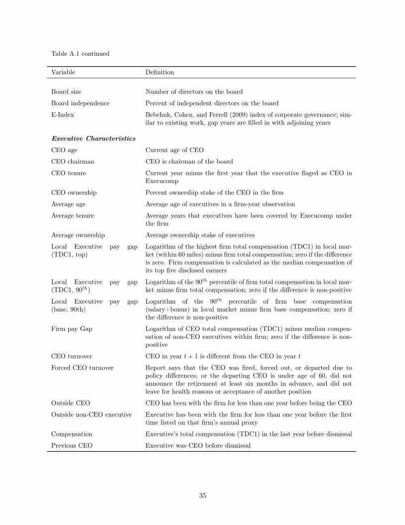
Table A.1 continued

Variable Definition

Board size Number of directors on the board

Board independence Percent of independent directors on the board

E-Index Bebchuk, Cohen, and Ferrell (2009) index of corporate governance; sim-ilar to existing work, gap years are filled in with adjoining years

Executive Characteristics

CEO age Current age of CEO

CEO chairman CEO is chairman of the board

CEO tenure Current year minus the first year that the executive flaged as CEO inExecucomp

CEO ownership Percent ownership stake of the CEO in the firm

Average age Average age of executives in a firm-year observation

Average tenure Average years that executives have been covered by Execucomp underthe firm

Average ownership Average ownership stake of executives

Local Executive pay gap(TDC1, top)

Logarithm of the highest firm total compensation (TDC1) in local mar-ket (within 60 miles) minus firm total compensation; zero if the differenceis zero. Firm compensation is calculated as the median compensation ofits top five disclosed earners

Local Executive pay gap(TDC1, 90th)

Logarithm of the 90th percentile of firm total compensation in local mar-ket minus firm total compensation; zero if the difference is non-positive

Local Executive pay gap(base, 90th)

Logarithm of the 90th percentile of firm base compensation(salary+bonus) in local market minus firm base compensation; zero ifthe difference is non-positive

Firm pay Gap Logarithm of CEO total compensation (TDC1) minus median compen-sation of non-CEO executives within firm; zero if the difference is non-positive

CEO turnover CEO in year t+ 1 is different from the CEO in year t

Forced CEO turnover Report says that the CEO was fired, forced out, or departed due topolicy differences; or the departing CEO is under age of 60, did notannounce the retirement at least six months in advance, and did notleave for health reasons or acceptance of another position

Outside CEO CEO has been with the firm for less than one year before being the CEO

Outside non-CEO executive Executive has been with the firm for less than one year before the firsttime listed on that firm’s annual proxy

Compensation Executive’s total compensation (TDC1) in the last year before dismissal

Previous CEO Executive was CEO before dismissal

35

Table A.1 continued

Variable Definition

Executive Departure and New Employment

Job change Executive’s employer in year t is different from his employer in year t+1

Promotion Executive moving to another Execucomp firm and new job’s compensa-tion (deflated by CPI) is higher than the old one’s or the new firm islarger than the old one in terms of total assets when compensation datais not available

Force The artical reporting the turnover uses words like "oust", "fired", "ter-minated" or overtly links turnover with poor performance or scandal, orthe leaving executive is paid with severance

Pursue The reason for departure is "to pursue other interests"

Retire The reason for departure is retirement

Resign If the turnover is not in any category above

New employment Executive obtains an executive position at a new firm within 3 yearsafter leaving the old firm

New employment public firm New firm is covered by Compustat database

New employment quality ad-justed

New employment public firm × log(1 + new firm total assets / old firmtotal assets) (CPI deflated)

Length of unemployment (First day in the new position − last day in the old position) / 365

36

Appendix B. Local Hiring Bias by Subsamples

I provide further evidence on local hiring bias by categorizing all hiring events into different

groups.

I first examine whether the cost and benefit of firm conducting a nationwide search or

executive moving long distance have any heterogeneous effect on the magnitude of the local

hiring bias. Results are presented in Table A.2. For brevity, I only show the results using

p1 as expected local hiring measure. Similar results are obtained if alternative measures are

used. Panel A categorizes sample hiring firms based on their S&P code. As the benefit

of finding a suitable leader is higher for larger firms, larger firms should be more likely to

hire executives from a nationwide executive pool. The results in Panel A offers evidence

supporting this argument. The local hiring bias is strongest, at 32.7%, for firms that are not

included in S&P 1500 index. The bias decreases to 30.0% for S&P SmallCap firms, further

decreases to 24.8% for MidCap firms, and becomes lowest for S&P 500 firms at 23.9%.28

Results remain qualitatively unchanged if I categorize sample hiring firms by size quintiles.

In Panel B, I examine whether local hirings happen less frequently for jobs with higher

payment. If compensation reflects the importance of the job, firms are more likely to con-

duct a nationwide search for that position. As for employees, higher monetary benefit is

more likely to overweigh the moving cost, and hence induces a long-distance move. For the

subsample where compensation data are available through Execucomp, I sort the full sample

into quintiles based on the total compensation (TDC1) that executives receive at the new

position. To control for the rapid compensation increase in the last two decades, I scale

each compensation with the average compensation level in that year. I find that jobs with

compensation at the lowest quintile have the highest local hiring bias at 30.7%. Such bias

gradually decreases as the compensation level rises. The bias for jobs with payment at the

highest quintile is 20.7%, which is significantly (at the 1% level) different from the bias at

the lowest quintile.

I also study whether the bias changes over time in Panel C. One might expect that with the

28The sample median total assets is 0.41 for firms not in S&P Index, 0.52 for SmallCap firms, 1.81 for MidCapfirms, and 11.52 for S&P 500 firms. All amounts are in billions of 2000 dollars.

37

increase in information and transportation convenience, firm’s searching cost and executive’s

moving cost would become lower in the latter sample period and thus the executive labor

market would become more integrated. However, I do not find such time pattern of the bias.

In fact, it seems that local hiring bias becomes more substantial in more recent years.

To investigate whether the local hiring bias only exists in the densest area (e.g. cities like

New York), I calculate the local hiring bias for all states. Results are illustrated in Figure

A.1. For the sake of statistical significance, I exclude states with less than 10 observations.

States are divided into quintiles based on their local hiring bias. First of all, firms in most

states exhibit significant bias toward local hiring. The bias is statistically significant at least

at the 5% level for all states not in the lowest quintile. Second, the local hiring bias is not only

driven by the states where firms cluster. The bottom part of Figure A.1 shows the geographic

pattern of firm density by grouping states into five categories based on the number of firms

in each state. Comparing Panels A and B, I find that although California, New York, and

Texas are in the top quintile of both bias and density, states with lower firm density, such as

Kansas, Oklahoma, and Oregon, also exhibit strong local hiring bias.

Finally, I categorize the sample based on hiring firm’s industry (Fama-French 30 industry

classification) and present the results in Table A.3. Results show that the local hiring bias

is prevalent across all industries and is between 20% to 30% for most of them. Among these

30 industries, utility as well as petroleum and natural gas industries have the largest bias.

One potential explanation is that the benefit from searching for a high quality executive is

relatively low for the energy industry.

Overall, the subsample analyses indicate that the local hiring bias is prevalent among

all industries, all markets with different density, all time periods, and even in the largest

firms and highest-paid positions. Also, the pattern of bias is consistent with the argument

that firms (executives) optimally choose to hire (move) locally based on the cost and benefit

analysis.

38

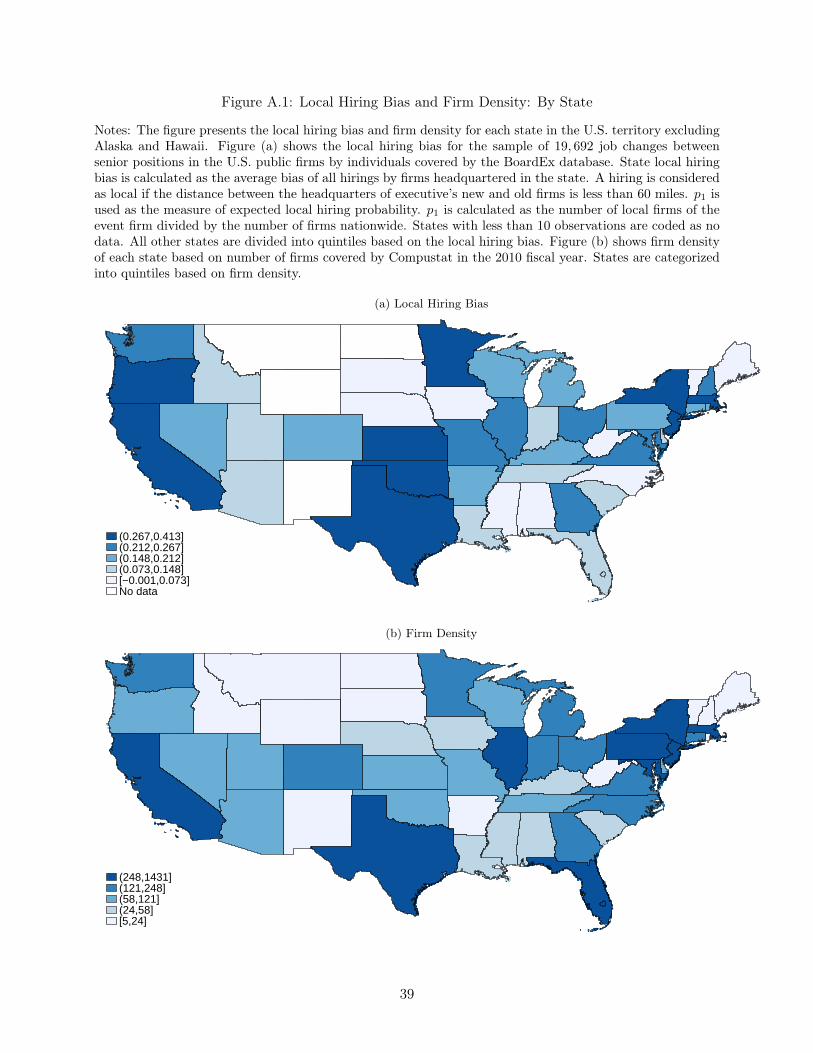
Figure A.1: Local Hiring Bias and Firm Density: By State

Notes: The figure presents the local hiring bias and firm density for each state in the U.S. territory excludingAlaska and Hawaii. Figure (a) shows the local hiring bias for the sample of 19, 692 job changes betweensenior positions in the U.S. public firms by individuals covered by the BoardEx database. State local hiringbias is calculated as the average bias of all hirings by firms headquartered in the state. A hiring is consideredas local if the distance between the headquarters of executive’s new and old firms is less than 60 miles. p1 isused as the measure of expected local hiring probability. p1 is calculated as the number of local firms of theevent firm divided by the number of firms nationwide. States with less than 10 observations are coded as nodata. All other states are divided into quintiles based on the local hiring bias. Figure (b) shows firm densityof each state based on number of firms covered by Compustat in the 2010 fiscal year. States are categorizedinto quintiles based on firm density.

(a) Local Hiring Bias

(0.267,0.413](0.212,0.267](0.148,0.212](0.073,0.148][−0.001,0.073]No data

(b) Firm Density

(248,1431](121,248](58,121](24,58][5,24]

39

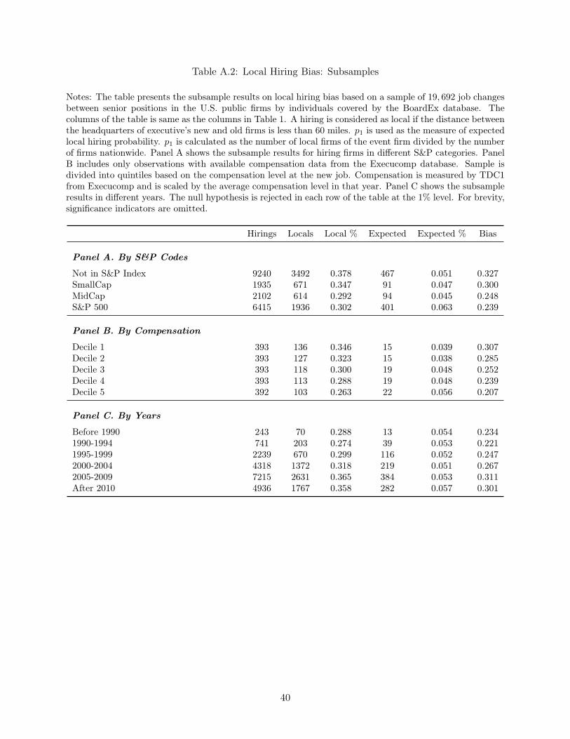
Table A.2: Local Hiring Bias: Subsamples

Notes: The table presents the subsample results on local hiring bias based on a sample of 19, 692 job changesbetween senior positions in the U.S. public firms by individuals covered by the BoardEx database. Thecolumns of the table is same as the columns in Table 1. A hiring is considered as local if the distance betweenthe headquarters of executive’s new and old firms is less than 60 miles. p1 is used as the measure of expectedlocal hiring probability. p1 is calculated as the number of local firms of the event firm divided by the numberof firms nationwide. Panel A shows the subsample results for hiring firms in different S&P categories. PanelB includes only observations with available compensation data from the Execucomp database. Sample isdivided into quintiles based on the compensation level at the new job. Compensation is measured by TDC1from Execucomp and is scaled by the average compensation level in that year. Panel C shows the subsampleresults in different years. The null hypothesis is rejected in each row of the table at the 1% level. For brevity,significance indicators are omitted.

Hirings Locals Local % Expected Expected % Bias

Panel A. By S&P Codes

Not in S&P Index 9240 3492 0.378 467 0.051 0.327SmallCap 1935 671 0.347 91 0.047 0.300MidCap 2102 614 0.292 94 0.045 0.248S&P 500 6415 1936 0.302 401 0.063 0.239

Panel B. By Compensation

Decile 1 393 136 0.346 15 0.039 0.307Decile 2 393 127 0.323 15 0.038 0.285Decile 3 393 118 0.300 19 0.048 0.252Decile 4 393 113 0.288 19 0.048 0.239Decile 5 392 103 0.263 22 0.056 0.207

Panel C. By Years

Before 1990 243 70 0.288 13 0.054 0.2341990-1994 741 203 0.274 39 0.053 0.2211995-1999 2239 670 0.299 116 0.052 0.2472000-2004 4318 1372 0.318 219 0.051 0.2672005-2009 7215 2631 0.365 384 0.053 0.311After 2010 4936 1767 0.358 282 0.057 0.301

40

Table A.3: Local Hiring Bias: By Industry

Notes: The table presents the results on local hiring bias by Fama-French 30 industries for the sample of 19, 692job changes between senior positions in the U.S. public firms by individuals covered by the BoardEx database.The columns of the table are same as the columns in Table 1. A hiring is considered as local if the distancebetween the headquarters of executive’s new and old firms is less than 60 miles. p1 is used as the measure ofexpected local hiring probability. p1 is calculated as the number of local firms of the event firm divided by thenumber of firms nationwide.

Hirings Locals Local % Expected Expected % Bias

Food products 399 71 0.178 15 0.038 0.140Beer and liquor 80 17 0.213 8 0.105 0.107Tobacco products 19 1 0.053 1 0.043 0.010Recreation 167 58 0.347 8 0.047 0.300Printing and publishing 138 72 0.522 9 0.067 0.455Consumer goods 324 85 0.262 15 0.047 0.215Apparel 266 69 0.259 15 0.056 0.204Healthcare and medical equipment 2590 954 0.368 166 0.064 0.304Chemicals 415 107 0.258 17 0.040 0.218Textiles 15 5 0.333 0 0.009 0.324Construction and construction materials 306 82 0.268 11 0.035 0.233Steel works 165 29 0.176 5 0.033 0.143Fabricated products and machinery 669 228 0.341 34 0.051 0.290Electrical equipment 129 31 0.240 4 0.030 0.210Automobiles and trucks 221 69 0.312 5 0.021 0.291Aircraft, ships, and railroad equipment 121 18 0.149 4 0.031 0.118Precious metals and industrial metal mining 57 14 0.246 1 0.024 0.221Coal 56 8 0.143 0 0.007 0.136Petroleum and natural gas 484 277 0.572 14 0.030 0.542Utilities 483 206 0.427 16 0.033 0.394Communication 518 157 0.303 29 0.056 0.247Personal and business services 3361 1126 0.335 202 0.060 0.275Business equipment 3565 1477 0.414 209 0.059 0.356Business supplies and shipping containers 238 36 0.151 6 0.025 0.126Transportation 286 84 0.294 11 0.038 0.255Wholesale 402 104 0.259 16 0.040 0.219Retail 1249 283 0.227 53 0.043 0.184Restaraunts, hotels, and motels 232 41 0.177 7 0.029 0.148Banking, insurance, real estate, and trading 2441 900 0.369 159 0.065 0.304Everything else 296 104 0.351 12 0.040 0.312

41

ReferencesAdams, R. B. and D. Ferreira (2007). A theory of friendly boards. Journal of Finance 62 (1),

217–250.

Adams, R. B. and D. Ferreira (2009). Women in the boardroom and their impact on governance

and performance. Journal of Financial Economics 94 (2), 291–309.

Almazan, A., A. De Motta, S. Titman, and V. Uysal (2010). Financial structure, acquisition oppor-

tunities, and firm locations. Journal of Finance 65 (2), 529–563.

Ang, J., G. Nagel, and J. Yang (2013). The effect of social pressures on CEO compensation. Working

Paper .

Bebchuk, L., A. Cohen, and A. Ferrell (2009). What matters in corporate governance? Review of

Financial Studies 22 (2), 783–827.

Bebchuk, L. A., M. Cremers, and U. C. Peyer (2011). The CEO pay slice. Journal of Financial

Economics 102 (1), 199–221.

Bouwman, C. (2013). The geography of executive compensation. Working Paper .

Cao, J., M. Lemmon, X. Pan, M. Qian, and G. Tian (2011). Political promotion, CEO incentives,

and the relationship between pay and performance. Working Paper .

Coles, J. L., N. D. Daniel, and L. Naveen (2008). Boards: Does one size fit all? Journal of Financial

Economics 87 (2), 329–356.

Coles, J. L., M. L. Lemmon, and J. F. Meschke (2012). Structural models and endogeneity in

corporate finance: The link between managerial ownership and corporate performance. Journal

of Financial Economics 103 (1), 149–168.

Coles, J. L., Z. F. Li, and Y. A. Wang (2013). Industry tournament incentives. Working Paper .

Costa, D. L. and M. E. Kahn (2000). Power couples: Changes in the locational choice of the college

educated, 1940-1990. Quarterly Journal of Economics 115 (4), 1287–1315.

42

Coughlan, A. T. and R. M. Schmidt (1985). Executive compensation, management turnover, and

firm performance: An empirical investigation. Journal of Accounting and Economics 7 (1), 43–66.

Demsetz, H. and B. Villalonga (2001). Ownership structure and corporate performance. Journal of

Corporate Finance 7 (3), 209–233.

Denis, D. J., D. K. Denis, and A. Sarin (1997). Ownership structure and top executive turnover.

Journal of Financial Economics 45 (2), 193–221.

Duranton, G. and D. Puga (2004). Micro-foundations of urban agglomeration economies. Handbook

of Regional and Urban Economics 4, 2063–2117.

Fahlenbrach, R., A. Low, and R. M. Stulz (2010). Why do firms appoint CEOs as outside directors?

Journal of Financial Economics 97 (1), 12–32.

Fee, C. E. and C. J. Hadlock (2003). Raids, rewards, and reputations in the market for managerial

talent. Review of Financial Studies 16 (4), 1315–1357.

Fee, C. E. and C. J. Hadlock (2004). Management turnover across the corporate hierarchy. Journal

of Accounting and Economics 37 (1), 3–38.

Francis, B., I. Hasan, K. John, and M. Waisman (forthcoming). Urban agglomeration and ceo

compensation. Journal of Financial and Quantitative Analysis.

Gibbons, R. and K. J. Murphy (1992). Optimal incentive contracts in the presence of career concerns:

Theory and evidence. Journal of Political Economy 100 (3), 468–505.

Glaeser, E. L. (1998). Are cities dying? Journal of Economic Perspectives 12 (2), 139–160.

Glaeser, E. L., H. D. Kallal, J. A. Scheinkman, and A. Shleifer (1992). Growth in cities. Journal of

Political Economy 100 (6), 1126–1152.

Gompers, P. A., J. L. Ishii, and A. Metrick (2003). Corporate governance and equity prices. Quarterly

Journal of Economics 118, 107–155.

Green, J. R. and N. Stokey (1983). A comparison of tournaments and contracts. Journal of Political

Economy 91 (3), 349–364.

43

Hadlock, C. J. and G. B. Lumer (1997). Compensation, turnover, and top management incentives:

Historical evidence*. The Journal of Business 70 (2), 153–187.

Hermalin, B. E. and M. S. Weisbach (1998). Endogenously chosen boards of directors and their

monitoring of the CEO. American Economic Review 88 (1), 96–118.

Holmes, T. J. (1999). Localization of industry and vertical disintegration. Review of Economics and

Statistics 81 (2), 314–325.

Hölmstrom, B. (1979). Moral hazard and observability. Bell Journal of Economics 10 (1), 74–91.

Huson, M. R., R. Parrino, and L. T. Starks (2001). Internal monitoring mechanisms and CEO

turnover: A long-term perspective. Journal of Finance 56 (6), 2265–2297.

Jaffe, A. B., M. Trajtenberg, and R. Henderson (1993). Geographic localization of knowledge

spillovers as evidenced by patent citations. Quarterly Journal of Economics 108 (3), 577–598.

Jensen, M. C. and K. J. Murphy (1990). Performance pay and top-management incentives. Journal

of Political Economy 98 (2), 225–264.

Jenter, D. and K. Lewellen (2014). Performance-induced CEO turnover. Working Paper .

John, K., A. Knyazeva, and D. Knyazeva (2011). Does geography matter? Firm location and

corporate payout policy. Journal of Financial Economics 101 (3), 533–551.

Kale, J. R., E. Reis, and A. Venkateswaran (2009). Rank-order tournaments and incentive alignment:

The effect on firm performance. Journal of Finance 64 (3), 1479–1512.

Kaplan, S. N. and B. A. Minton (2012). How has CEO turnover changed? International Review of

Finance 12 (1), 57–87.

Kedia, S. and S. Rajgopal (2009). Neighborhood matters: The impact of location on broad based

stock option plans. Journal of Financial Economics 92 (1), 109–127.

Kini, O. and R. Williams (2012). Tournament incentives, firm risk, and corporate policies. Journal

of Financial Economics 103 (2), 350–376.

44

Knyazeva, A., D. Knyazeva, and R. W. Masulis (2013). The supply of corporate directors and board

independence. Review of Financial Studies 26 (6), 1561–1605.

Lazear, E. P. and S. Rosen (1981). Rank-order tournaments as optimum labor contracts. Journal

of Political Economy 89 (5), 841–864.

Marshall, A. (1920). Principles of Economics. London: MacMillan.

Masulis, R. W. and S. Mobbs (2014). Independent director incentives: Where do talented directors

spend their limited time and energy? Journal of Financial Economics 111 (2), 406–429.

McConnell, J. J. and H. Servaes (1990). Additional evidence on equity ownership and corporate

value. Journal of Financial Economics 27 (2), 595–612.

Morck, R., A. Shleifer, and R. W. Vishny (1988). Management ownership and market valuation:

An empirical analysis. Journal of Financial Economics 20, 293–315.

Murphy, K. J. (1999). Executive compensation. Handbook of Labor Economics 3, 2485–2563.

Parrino, R. (1997). CEO turnover and outside succession a cross-sectional analysis. Journal of

Financial Economics 46 (2), 165–197.

Pool, V. K., N. Stoffman, and S. E. Yonker (forthcoming). The people in your neighborhood: Social

interactions and mutual fund portfolios. Journal of Finance.

Rosenthal, S. S. and W. C. Strange (2004). Evidence on the nature and sources of agglomeration

economies. Handbook of Regional and Urban Economics 4, 2119–2171.

Shaver, J. M. and F. Flyer (2000). Agglomeration economies, firm heterogeneity, and foreign direct

investment in the united states. Strategic Management Journal 21 (12), 1175–1194.

Tabuchi, T. (1998). Urban agglomeration and dispersion: A synthesis of Alonso and Krugman.

Journal of Urban Economics 44 (3), 333–351.

Uysal, V. B., S. Kedia, and V. Panchapagesan (2008). Geography and acquirer returns. Journal of

Financial Intermediation 17 (2), 256–275.

45

Warner, J. B., R. L. Watts, and K. H. Wruck (1988). Stock prices and top management changes.

Journal of Financial Economics 20, 461–492.

Weisbach, M. S. (1988). Outside directors and CEO turnover. Journal of Financial Economics 20,

431–460.

Yermack, D. (2004). Remuneration, retention, and reputation incentives for outside directors. The

Journal of Finance 59 (5), 2281–2308.

Yonker, S. E. (2014). Geography and the market for CEOs. Working Paper .

46

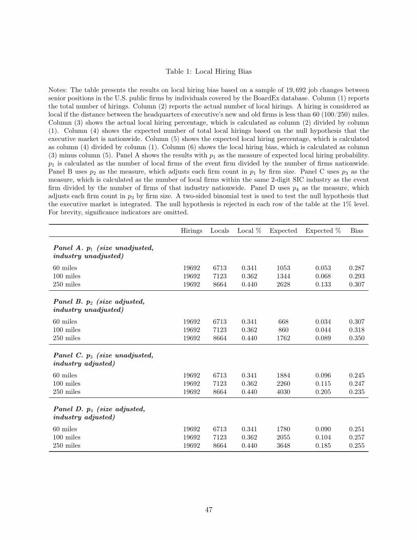
Table 1: Local Hiring Bias

Notes: The table presents the results on local hiring bias based on a sample of 19, 692 job changes betweensenior positions in the U.S. public firms by individuals covered by the BoardEx database. Column (1) reportsthe total number of hirings. Column (2) reports the actual number of local hirings. A hiring is considered aslocal if the distance between the headquarters of executive’s new and old firms is less than 60 (100/250) miles.Column (3) shows the actual local hiring percentage, which is calculated as column (2) divided by column(1). Column (4) shows the expected number of total local hirings based on the null hypothesis that theexecutive market is nationwide. Column (5) shows the expected local hiring percentage, which is calculatedas column (4) divided by column (1). Column (6) shows the local hiring bias, which is calculated as column(3) minus column (5). Panel A shows the results with p1 as the measure of expected local hiring probability.p1 is calculated as the number of local firms of the event firm divided by the number of firms nationwide.Panel B uses p2 as the measure, which adjusts each firm count in p1 by firm size. Panel C uses p3 as themeasure, which is calculated as the number of local firms within the same 2-digit SIC industry as the eventfirm divided by the number of firms of that industry nationwide. Panel D uses p4 as the measure, whichadjusts each firm count in p3 by firm size. A two-sided binomial test is used to test the null hypothesis thatthe executive market is integrated. The null hypothesis is rejected in each row of the table at the 1% level.For brevity, significance indicators are omitted.

Hirings Locals Local % Expected Expected % Bias

Panel A. p1 (size unadjusted,industry unadjusted)

60 miles 19692 6713 0.341 1053 0.053 0.287100 miles 19692 7123 0.362 1344 0.068 0.293250 miles 19692 8664 0.440 2628 0.133 0.307

Panel B. p2 (size adjusted,industry unadjusted)

60 miles 19692 6713 0.341 668 0.034 0.307100 miles 19692 7123 0.362 860 0.044 0.318250 miles 19692 8664 0.440 1762 0.089 0.350

Panel C. p3 (size unadjusted,industry adjusted)

60 miles 19692 6713 0.341 1884 0.096 0.245100 miles 19692 7123 0.362 2260 0.115 0.247250 miles 19692 8664 0.440 4030 0.205 0.235

Panel D. p4 (size adjusted,industry adjusted)

60 miles 19692 6713 0.341 1780 0.090 0.251100 miles 19692 7123 0.362 2055 0.104 0.257250 miles 19692 8664 0.440 3648 0.185 0.255

47

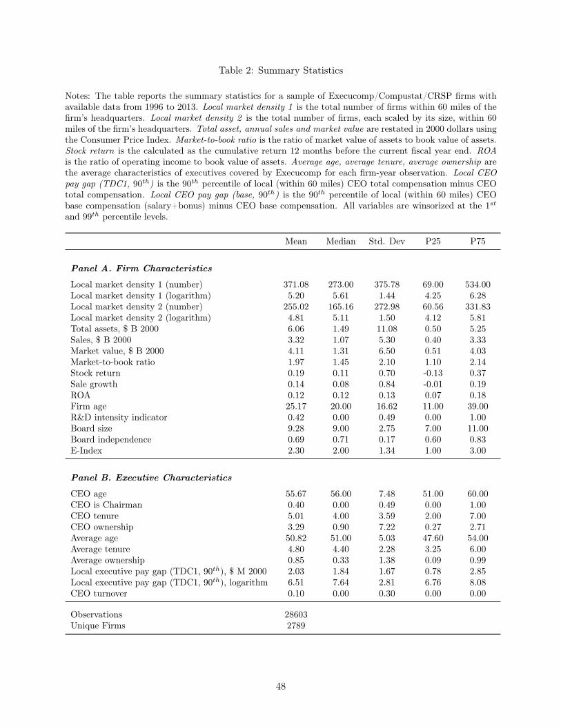
Table 2: Summary Statistics

Notes: The table reports the summary statistics for a sample of Execucomp/Compustat/CRSP firms withavailable data from 1996 to 2013. Local market density 1 is the total number of firms within 60 miles of thefirm’s headquarters. Local market density 2 is the total number of firms, each scaled by its size, within 60miles of the firm’s headquarters. Total asset, annual sales and market value are restated in 2000 dollars usingthe Consumer Price Index. Market-to-book ratio is the ratio of market value of assets to book value of assets.Stock return is the calculated as the cumulative return 12 months before the current fiscal year end. ROAis the ratio of operating income to book value of assets. Average age, average tenure, average ownership arethe average characteristics of executives covered by Execucomp for each firm-year observation. Local CEOpay gap (TDC1, 90th) is the 90th percentile of local (within 60 miles) CEO total compensation minus CEOtotal compensation. Local CEO pay gap (base, 90th) is the 90th percentile of local (within 60 miles) CEObase compensation (salary+bonus) minus CEO base compensation. All variables are winsorized at the 1st

and 99th percentile levels.

Mean Median Std. Dev P25 P75

Panel A. Firm Characteristics

Local market density 1 (number) 371.08 273.00 375.78 69.00 534.00Local market density 1 (logarithm) 5.20 5.61 1.44 4.25 6.28Local market density 2 (number) 255.02 165.16 272.98 60.56 331.83Local market density 2 (logarithm) 4.81 5.11 1.50 4.12 5.81Total assets, $ B 2000 6.06 1.49 11.08 0.50 5.25Sales, $ B 2000 3.32 1.07 5.30 0.40 3.33Market value, $ B 2000 4.11 1.31 6.50 0.51 4.03Market-to-book ratio 1.97 1.45 2.10 1.10 2.14Stock return 0.19 0.11 0.70 -0.13 0.37Sale growth 0.14 0.08 0.84 -0.01 0.19ROA 0.12 0.12 0.13 0.07 0.18Firm age 25.17 20.00 16.62 11.00 39.00R&D intensity indicator 0.42 0.00 0.49 0.00 1.00Board size 9.28 9.00 2.75 7.00 11.00Board independence 0.69 0.71 0.17 0.60 0.83E-Index 2.30 2.00 1.34 1.00 3.00

Panel B. Executive Characteristics

CEO age 55.67 56.00 7.48 51.00 60.00CEO is Chairman 0.40 0.00 0.49 0.00 1.00CEO tenure 5.01 4.00 3.59 2.00 7.00CEO ownership 3.29 0.90 7.22 0.27 2.71Average age 50.82 51.00 5.03 47.60 54.00Average tenure 4.80 4.40 2.28 3.25 6.00Average ownership 0.85 0.33 1.38 0.09 0.99Local executive pay gap (TDC1, 90th), $ M 2000 2.03 1.84 1.67 0.78 2.85Local executive pay gap (TDC1, 90th), logarithm 6.51 7.64 2.81 6.76 8.08CEO turnover 0.10 0.00 0.30 0.00 0.00

Observations 28603Unique Firms 2789

48

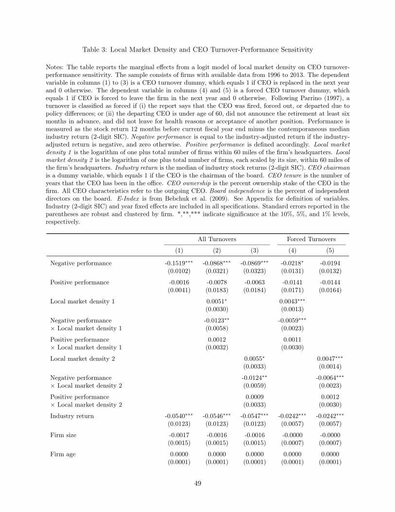
Table 3: Local Market Density and CEO Turnover-Performance Sensitivity

Notes: The table reports the marginal effects from a logit model of local market density on CEO turnover-performance sensitivity. The sample consists of firms with available data from 1996 to 2013. The dependentvariable in columns (1) to (3) is a CEO turnover dummy, which equals 1 if CEO is replaced in the next yearand 0 otherwise. The dependent variable in columns (4) and (5) is a forced CEO turnover dummy, whichequals 1 if CEO is forced to leave the firm in the next year and 0 otherwise. Following Parrino (1997), aturnover is classified as forced if (i) the report says that the CEO was fired, forced out, or departed due topolicy differences; or (ii) the departing CEO is under age of 60, did not announce the retirement at least sixmonths in advance, and did not leave for health reasons or acceptance of another position. Performance ismeasured as the stock return 12 months before current fiscal year end minus the contemporaneous medianindustry return (2-digit SIC). Negative performance is equal to the industry-adjusted return if the industry-adjusted return is negative, and zero otherwise. Positive performance is defined accordingly. Local marketdensity 1 is the logarithm of one plus total number of firms within 60 miles of the firm’s headquarters. Localmarket density 2 is the logarithm of one plus total number of firms, each scaled by its size, within 60 miles ofthe firm’s headquarters. Industry return is the median of industry stock returns (2-digit SIC). CEO chairmanis a dummy variable, which equals 1 if the CEO is the chairman of the board. CEO tenure is the number ofyears that the CEO has been in the office. CEO ownership is the percent ownership stake of the CEO in thefirm. All CEO characteristics refer to the outgoing CEO. Board independence is the percent of independentdirectors on the board. E-Index is from Bebchuk et al. (2009). See Appendix for definition of variables.Industry (2-digit SIC) and year fixed effects are included in all specifications. Standard errors reported in theparentheses are robust and clustered by firm. *,**,*** indicate significance at the 10%, 5%, and 1% levels,respectively.

All Turnovers Forced Turnovers

(1) (2) (3) (4) (5)

Negative performance -0.1519∗∗∗ -0.0868∗∗∗ -0.0869∗∗∗ -0.0218∗ -0.0194(0.0102) (0.0321) (0.0323) (0.0131) (0.0132)

Positive performance -0.0016 -0.0078 -0.0063 -0.0141 -0.0144(0.0041) (0.0183) (0.0184) (0.0171) (0.0164)

Local market density 1 0.0051∗ 0.0043∗∗∗

(0.0030) (0.0013)

Negative performance -0.0123∗∗ -0.0059∗∗∗

× Local market density 1 (0.0058) (0.0023)

Positive performance 0.0012 0.0011× Local market density 1 (0.0032) (0.0030)

Local market density 2 0.0055∗ 0.0047∗∗∗

(0.0033) (0.0014)

Negative performance -0.0124∗∗ -0.0064∗∗∗

× Local market density 2 (0.0059) (0.0023)

Positive performance 0.0009 0.0012× Local market density 2 (0.0033) (0.0030)

Industry return -0.0540∗∗∗ -0.0546∗∗∗ -0.0547∗∗∗ -0.0242∗∗∗ -0.0242∗∗∗

(0.0123) (0.0123) (0.0123) (0.0057) (0.0057)

Firm size -0.0017 -0.0016 -0.0016 -0.0000 -0.0000(0.0015) (0.0015) (0.0015) (0.0007) (0.0007)

Firm age 0.0000 0.0000 0.0000 0.0000 0.0000(0.0001) (0.0001) (0.0001) (0.0001) (0.0001)

49

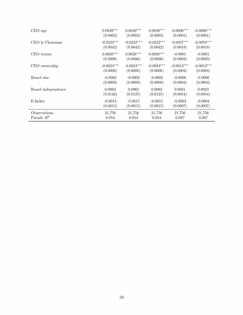
CEO age 0.0049∗∗∗ 0.0049∗∗∗ 0.0049∗∗∗ -0.0006∗∗∗ -0.0006∗∗∗

(0.0003) (0.0003) (0.0003) (0.0001) (0.0001)

CEO is Chairman -0.0223∗∗∗ -0.0222∗∗∗ -0.0222∗∗∗ -0.0057∗∗∗ -0.0058∗∗∗

(0.0042) (0.0042) (0.0042) (0.0018) (0.0018)

CEO tenure 0.0028∗∗∗ 0.0028∗∗∗ 0.0028∗∗∗ -0.0001 -0.0001(0.0006) (0.0006) (0.0006) (0.0003) (0.0003)

CEO ownership -0.0024∗∗∗ -0.0024∗∗∗ -0.0024∗∗∗ -0.0013∗∗∗ -0.0013∗∗∗

(0.0006) (0.0006) (0.0006) (0.0004) (0.0004)

Board size -0.0002 -0.0002 -0.0002 -0.0006 -0.0006(0.0009) (0.0009) (0.0009) (0.0004) (0.0004)

Board independence 0.0063 0.0062 0.0062 0.0021 0.0023(0.0126) (0.0125) (0.0125) (0.0054) (0.0054)

E-Index -0.0014 -0.0015 -0.0015 -0.0004 -0.0004(0.0015) (0.0015) (0.0015) (0.0007) (0.0007)

Observations 21,756 21,756 21,756 21,756 21,756Pseudo R2 0.054 0.054 0.054 0.087 0.087

50

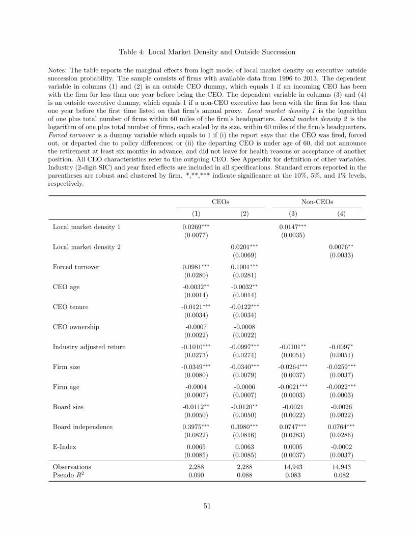
Table 4: Local Market Density and Outside Succession

Notes: The table reports the marginal effects from logit model of local market density on executive outsidesuccession probability. The sample consists of firms with available data from 1996 to 2013. The dependentvariable in columns (1) and (2) is an outside CEO dummy, which equals 1 if an incoming CEO has beenwith the firm for less than one year before being the CEO. The dependent variable in columns (3) and (4)is an outside executive dummy, which equals 1 if a non-CEO executive has been with the firm for less thanone year before the first time listed on that firm’s annual proxy. Local market density 1 is the logarithmof one plus total number of firms within 60 miles of the firm’s headquarters. Local market density 2 is thelogarithm of one plus total number of firms, each scaled by its size, within 60 miles of the firm’s headquarters.Forced turnover is a dummy variable which equals to 1 if (i) the report says that the CEO was fired, forcedout, or departed due to policy differences; or (ii) the departing CEO is under age of 60, did not announcethe retirement at least six months in advance, and did not leave for health reasons or acceptance of anotherposition. All CEO characteristics refer to the outgoing CEO. See Appendix for definition of other variables.Industry (2-digit SIC) and year fixed effects are included in all specifications. Standard errors reported in theparentheses are robust and clustered by firm. *,**,*** indicate significance at the 10%, 5%, and 1% levels,respectively.

CEOs Non-CEOs

(1) (2) (3) (4)

Local market density 1 0.0269∗∗∗ 0.0147∗∗∗

(0.0077) (0.0035)

Local market density 2 0.0201∗∗∗ 0.0076∗∗

(0.0069) (0.0033)

Forced turnover 0.0981∗∗∗ 0.1001∗∗∗

(0.0280) (0.0281)

CEO age -0.0032∗∗ -0.0032∗∗

(0.0014) (0.0014)

CEO tenure -0.0121∗∗∗ -0.0122∗∗∗

(0.0034) (0.0034)

CEO ownership -0.0007 -0.0008(0.0022) (0.0022)

Industry adjusted return -0.1010∗∗∗ -0.0997∗∗∗ -0.0101∗∗ -0.0097∗

(0.0273) (0.0274) (0.0051) (0.0051)

Firm size -0.0349∗∗∗ -0.0340∗∗∗ -0.0264∗∗∗ -0.0259∗∗∗

(0.0080) (0.0079) (0.0037) (0.0037)

Firm age -0.0004 -0.0006 -0.0021∗∗∗ -0.0022∗∗∗

(0.0007) (0.0007) (0.0003) (0.0003)

Board size -0.0112∗∗ -0.0120∗∗ -0.0021 -0.0026(0.0050) (0.0050) (0.0022) (0.0022)

Board independence 0.3975∗∗∗ 0.3980∗∗∗ 0.0747∗∗∗ 0.0764∗∗∗

(0.0822) (0.0816) (0.0283) (0.0286)

E-Index 0.0065 0.0063 0.0005 -0.0002(0.0085) (0.0085) (0.0037) (0.0037)

Observations 2,288 2,288 14,943 14,943Pseudo R2 0.090 0.088 0.083 0.082

51

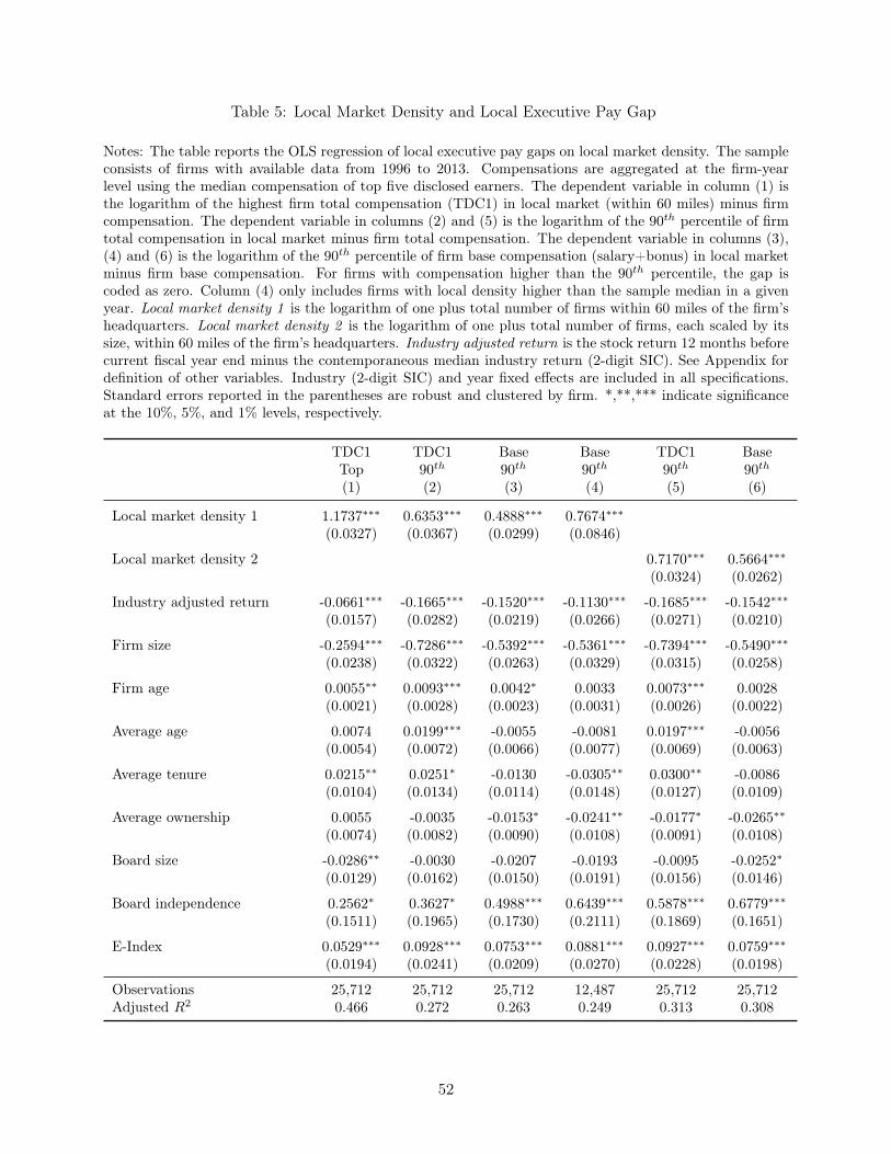
Table 5: Local Market Density and Local Executive Pay Gap

Notes: The table reports the OLS regression of local executive pay gaps on local market density. The sampleconsists of firms with available data from 1996 to 2013. Compensations are aggregated at the firm-yearlevel using the median compensation of top five disclosed earners. The dependent variable in column (1) isthe logarithm of the highest firm total compensation (TDC1) in local market (within 60 miles) minus firmcompensation. The dependent variable in columns (2) and (5) is the logarithm of the 90th percentile of firmtotal compensation in local market minus firm total compensation. The dependent variable in columns (3),(4) and (6) is the logarithm of the 90th percentile of firm base compensation (salary+bonus) in local marketminus firm base compensation. For firms with compensation higher than the 90th percentile, the gap iscoded as zero. Column (4) only includes firms with local density higher than the sample median in a givenyear. Local market density 1 is the logarithm of one plus total number of firms within 60 miles of the firm’sheadquarters. Local market density 2 is the logarithm of one plus total number of firms, each scaled by itssize, within 60 miles of the firm’s headquarters. Industry adjusted return is the stock return 12 months beforecurrent fiscal year end minus the contemporaneous median industry return (2-digit SIC). See Appendix fordefinition of other variables. Industry (2-digit SIC) and year fixed effects are included in all specifications.Standard errors reported in the parentheses are robust and clustered by firm. *,**,*** indicate significanceat the 10%, 5%, and 1% levels, respectively.

TDC1 TDC1 Base Base TDC1 BaseTop 90th 90th 90th 90th 90th

(1) (2) (3) (4) (5) (6)

Local market density 1 1.1737∗∗∗ 0.6353∗∗∗ 0.4888∗∗∗ 0.7674∗∗∗

(0.0327) (0.0367) (0.0299) (0.0846)

Local market density 2 0.7170∗∗∗ 0.5664∗∗∗

(0.0324) (0.0262)

Industry adjusted return -0.0661∗∗∗ -0.1665∗∗∗ -0.1520∗∗∗ -0.1130∗∗∗ -0.1685∗∗∗ -0.1542∗∗∗

(0.0157) (0.0282) (0.0219) (0.0266) (0.0271) (0.0210)

Firm size -0.2594∗∗∗ -0.7286∗∗∗ -0.5392∗∗∗ -0.5361∗∗∗ -0.7394∗∗∗ -0.5490∗∗∗

(0.0238) (0.0322) (0.0263) (0.0329) (0.0315) (0.0258)

Firm age 0.0055∗∗ 0.0093∗∗∗ 0.0042∗ 0.0033 0.0073∗∗∗ 0.0028(0.0021) (0.0028) (0.0023) (0.0031) (0.0026) (0.0022)

Average age 0.0074 0.0199∗∗∗ -0.0055 -0.0081 0.0197∗∗∗ -0.0056(0.0054) (0.0072) (0.0066) (0.0077) (0.0069) (0.0063)

Average tenure 0.0215∗∗ 0.0251∗ -0.0130 -0.0305∗∗ 0.0300∗∗ -0.0086(0.0104) (0.0134) (0.0114) (0.0148) (0.0127) (0.0109)

Average ownership 0.0055 -0.0035 -0.0153∗ -0.0241∗∗ -0.0177∗ -0.0265∗∗

(0.0074) (0.0082) (0.0090) (0.0108) (0.0091) (0.0108)

Board size -0.0286∗∗ -0.0030 -0.0207 -0.0193 -0.0095 -0.0252∗

(0.0129) (0.0162) (0.0150) (0.0191) (0.0156) (0.0146)

Board independence 0.2562∗ 0.3627∗ 0.4988∗∗∗ 0.6439∗∗∗ 0.5878∗∗∗ 0.6779∗∗∗

(0.1511) (0.1965) (0.1730) (0.2111) (0.1869) (0.1651)

E-Index 0.0529∗∗∗ 0.0928∗∗∗ 0.0753∗∗∗ 0.0881∗∗∗ 0.0927∗∗∗ 0.0759∗∗∗

(0.0194) (0.0241) (0.0209) (0.0270) (0.0228) (0.0198)

Observations 25,712 25,712 25,712 12,487 25,712 25,712Adjusted R2 0.466 0.272 0.263 0.249 0.313 0.308

52

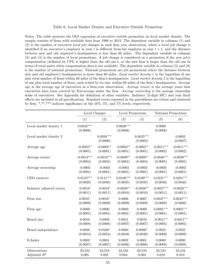
Table 6: Local Market Density and Executive Outside Promotion

Notes: The table presents the OLS regression of executive outside promotion on local market density. Thesample consists of firms with available data from 1996 to 2013. The dependent variable in columns (1) and(2) is the number of executive local job changes in each firm year observation, where a local job change isidentified if an executive’s employer in year t is different from his employer in year t + 1, and the distancebetween new and old employer’s headquarters is less than 60 miles. The dependent variable in columns(3) and (4) is the number of local promotions. A job change is considered as a promotion if the new job’scompensation (deflated by CPI) is higher than the old one’s, or the new firm is larger than the old one interms of total assets when compensation data is not available. The dependent variable in columns (5) and (6)is the number of national promotions. National promotions are job promotions where the distance betweennew and old employer’s headquarters is more than 60 miles. Local market density 1 is the logarithm of oneplus total number of firms within 60 miles of the firm’s headquarters. Local market density 2 is the logarithmof one plus total number of firms, each scaled by its size, within 60 miles of the firm’s headquarters. Averageage is the average age of executives in a firm-year observation. Average tenure is the average years thatexecutives have been covered by Execucomp under the firm. Average ownership is the average ownershipstake of executives. See Appendix for definition of other variables. Industry (2-digit SIC) and year fixedeffects are included in all specifications. Standard errors reported in the parentheses are robust and clusteredby firm. *,**,*** indicate significance at the 10%, 5%, and 1% levels, respectively.

Local Changes Local Promotions National Promotions

(1) (2) (3) (4) (5) (6)

Local market density 1 0.0043∗∗∗ 0.0038∗∗∗ 0.0009(0.0006) (0.0006) (0.0008)

Local market density 2 0.0038∗∗∗ 0.0035∗∗∗ 0.0003(0.0006) (0.0005) (0.0007)

Average age -0.0003∗∗ -0.0003∗∗ -0.0003∗∗ -0.0003∗∗ -0.0011∗∗∗ -0.0011∗∗∗

(0.0001) (0.0001) (0.0001) (0.0001) (0.0002) (0.0002)

Average tenure -0.0013∗∗∗ -0.0013∗∗∗ -0.0009∗∗ -0.0009∗∗ -0.0040∗∗∗ -0.0039∗∗∗

(0.0004) (0.0004) (0.0004) (0.0004) (0.0005) (0.0005)

Average ownership -0.0002 -0.0002 -0.0002 -0.0002 -0.0002 -0.0002(0.0001) (0.0001) (0.0001) (0.0001) (0.0001) (0.0001)

CEO turnover 0.0110∗∗∗ 0.0111∗∗∗ 0.0109∗∗∗ 0.0109∗∗∗ 0.0231∗∗∗ 0.0231∗∗∗

(0.0038) (0.0038) (0.0035) (0.0035) (0.0046) (0.0046)

Industry adjusted return -0.0018∗ -0.0018∗ -0.0020∗∗ -0.0020∗∗ -0.0027∗∗∗ -0.0028∗∗∗

(0.0011) (0.0011) (0.0010) (0.0010) (0.0011) (0.0011)

Firm size 0.0016∗ 0.0016∗ 0.0006 0.0007 0.0047∗∗∗ 0.0047∗∗∗

(0.0009) (0.0009) (0.0009) (0.0009) (0.0008) (0.0008)

Firm age 0.0000 0.0000 0.0000 0.0000 0.0005∗∗∗ 0.0005∗∗∗

(0.0001) (0.0001) (0.0001) (0.0001) (0.0001) (0.0001)

Board size 0.0010 0.0009 0.0011 0.0010 -0.0011∗∗ -0.0011∗∗

(0.0008) (0.0008) (0.0007) (0.0007) (0.0005) (0.0005)

Board independence 0.0088 0.0100∗ 0.0080 0.0090∗ 0.0025 0.0025(0.0054) (0.0054) (0.0049) (0.0049) (0.0069) (0.0069)

E-Index 0.0002 0.0001 0.0002 0.0001 0.0000 0.0000(0.0007) (0.0007) (0.0006) (0.0006) (0.0008) (0.0008)

Observations 23,534 23,534 23,534 23,534 23,534 23,534Adjusted R2 0.005 0.005 0.004 0.004 0.010 0.010

53

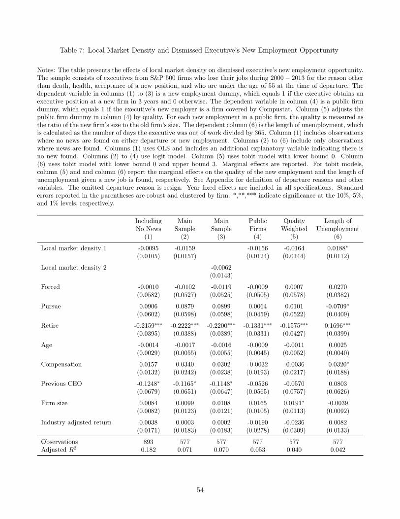
Table 7: Local Market Density and Dismissed Executive’s New Employment Opportunity

Notes: The table presents the effects of local market density on dismissed executive’s new employment opportunity.The sample consists of executives from S&P 500 firms who lose their jobs during 2000− 2013 for the reason otherthan death, health, acceptance of a new position, and who are under the age of 55 at the time of departure. Thedependent variable in columns (1) to (3) is a new employment dummy, which equals 1 if the executive obtains anexecutive position at a new firm in 3 years and 0 otherwise. The dependent variable in column (4) is a public firmdummy, which equals 1 if the executive’s new employer is a firm covered by Compustat. Column (5) adjusts thepublic firm dummy in column (4) by quality. For each new employment in a public firm, the quality is measured asthe ratio of the new firm’s size to the old firm’s size. The dependent column (6) is the length of unemployment, whichis calculated as the number of days the executive was out of work divided by 365. Column (1) includes observationswhere no news are found on either departure or new employment. Columns (2) to (6) include only observationswhere news are found. Columns (1) uses OLS and includes an additional explanatory variable indicating there isno new found. Columns (2) to (4) use logit model. Column (5) uses tobit model with lower bound 0. Column(6) uses tobit model with lower bound 0 and upper bound 3. Marginal effects are reported. For tobit models,column (5) and and column (6) report the marginal effects on the quality of the new employment and the length ofunemployment given a new job is found, respectively. See Appendix for definition of departure reasons and othervariables. The omitted departure reason is resign. Year fixed effects are included in all specifications. Standarderrors reported in the parentheses are robust and clustered by firm. *,**,*** indicate significance at the 10%, 5%,and 1% levels, respectively.

Including Main Main Public Quality Length ofNo News Sample Sample Firms Weighted Unemployment

(1) (2) (3) (4) (5) (6)

Local market density 1 -0.0095 -0.0159 -0.0156 -0.0164 0.0188∗

(0.0105) (0.0157) (0.0124) (0.0144) (0.0112)

Local market density 2 -0.0062(0.0143)

Forced -0.0010 -0.0102 -0.0119 -0.0009 0.0007 0.0270(0.0582) (0.0527) (0.0525) (0.0505) (0.0578) (0.0382)

Pursue 0.0906 0.0879 0.0899 0.0064 0.0101 -0.0709∗

(0.0602) (0.0598) (0.0598) (0.0459) (0.0522) (0.0409)

Retire -0.2159∗∗∗ -0.2222∗∗∗ -0.2200∗∗∗ -0.1331∗∗∗ -0.1575∗∗∗ 0.1696∗∗∗

(0.0395) (0.0388) (0.0389) (0.0331) (0.0427) (0.0399)

Age -0.0014 -0.0017 -0.0016 -0.0009 -0.0011 0.0025(0.0029) (0.0055) (0.0055) (0.0045) (0.0052) (0.0040)

Compensation 0.0157 0.0340 0.0302 -0.0032 -0.0036 -0.0320∗

(0.0132) (0.0242) (0.0238) (0.0193) (0.0217) (0.0188)

Previous CEO -0.1248∗ -0.1165∗ -0.1148∗ -0.0526 -0.0570 0.0803(0.0679) (0.0651) (0.0647) (0.0565) (0.0757) (0.0626)

Firm size 0.0084 0.0099 0.0108 0.0165 0.0191∗ -0.0039(0.0082) (0.0123) (0.0121) (0.0105) (0.0113) (0.0092)

Industry adjusted return 0.0038 0.0003 0.0002 -0.0190 -0.0236 0.0082(0.0171) (0.0183) (0.0183) (0.0278) (0.0309) (0.0133)

Observations 893 577 577 577 577 577Adjusted R2 0.182 0.071 0.070 0.053 0.040 0.042

54

Table 8: Local Hiring Bias of Dismissed Executives

Notes: The table presents the local hiring percentage for a sample of dismissed executives who find a newjob in a public firm within a three-year window. The sample of dismissed executives is same as the sampleused in Table 7. Panel A shows the realized local hiring percentage and local hiring bias for the sample ofdismissed executives. The columns are same as the columns in Table 1. Four different measures of expectedlocal hiring probability and three distance cutoffs are used. See Table 1 for details. Panel B compares thelocal hiring bias between the dismissed sample and the “non-dismissed” sample. The “non-dismissed” sampleis the 19, 692 executive job changes covered by the BoardEx database used in Table 1. Columns (1) and (2)report the mean local hiring bias for the dismissed and the “non-dismissed” samples, respectively. Column(3) shows the difference between columns (1) and (2). Column (4) shows the t-statistic of a mean comparisontest on local hiring bias between the dismissed and the “non-dismissed” sample under the assumption ofunequal variance.

Panel A. Local Hiring Bias: Dismissed Sample

Hirings Locals Local % Expected Expected % Bias

p1, 60-mile 105 21 0.200 5 0.051 0.149p2, 60-mile 105 21 0.200 3 0.032 0.168p3, 60-mile 105 21 0.200 11 0.105 0.095p4, 60-mile 105 21 0.200 11 0.103 0.097

p1, 100-mile 105 23 0.219 7 0.064 0.155p2, 100-mile 105 23 0.219 4 0.040 0.179p3, 100-mile 105 23 0.219 13 0.120 0.099p4, 100-mile 105 23 0.219 12 0.110 0.109

p1, 250-mile 105 35 0.333 13 0.122 0.212p2, 250-mile 105 35 0.333 8 0.080 0.253p3, 250-mile 105 35 0.333 23 0.217 0.117p4, 250-mile 105 35 0.333 19 0.185 0.149

Panel B. Comparison between Dismissed and "Non-Dismissed" Samples

Bias: Dismissed Bias: "Non-Dismissed" Difference t-stat

p1, 60-mile 0.149 0.287 -0.138 3.57p2, 60-mile 0.168 0.307 -0.139 3.55p3, 60-mile 0.095 0.245 -0.150 3.55p4, 60-mile 0.097 0.251 -0.153 3.31

p1, 100-mile 0.155 0.293 -0.139 3.45p2, 100-mile 0.179 0.318 -0.139 3.45p3, 100-mile 0.099 0.247 -0.148 3.36p4, 100-mile 0.109 0.257 -0.149 3.13

p1, 250-mile 0.212 0.307 -0.095 2.07p2, 250-mile 0.253 0.350 -0.098 2.14p3, 250-mile 0.117 0.235 -0.119 2.28p4, 250-mile 0.149 0.255 -0.106 1.93

55

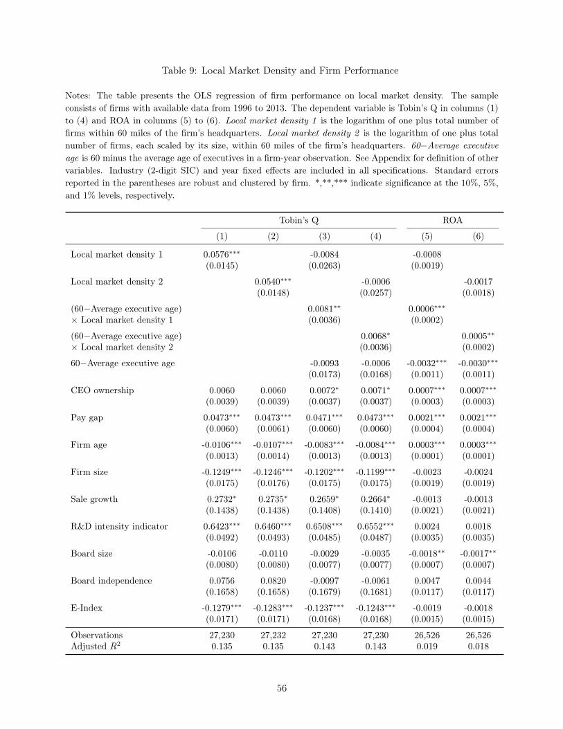
Table 9: Local Market Density and Firm Performance

Notes: The table presents the OLS regression of firm performance on local market density. The sampleconsists of firms with available data from 1996 to 2013. The dependent variable is Tobin’s Q in columns (1)to (4) and ROA in columns (5) to (6). Local market density 1 is the logarithm of one plus total number offirms within 60 miles of the firm’s headquarters. Local market density 2 is the logarithm of one plus totalnumber of firms, each scaled by its size, within 60 miles of the firm’s headquarters. 60−Average executiveage is 60 minus the average age of executives in a firm-year observation. See Appendix for definition of othervariables. Industry (2-digit SIC) and year fixed effects are included in all specifications. Standard errorsreported in the parentheses are robust and clustered by firm. *,**,*** indicate significance at the 10%, 5%,

and 1% levels, respectively.

Tobin’s Q ROA

(1) (2) (3) (4) (5) (6)

Local market density 1 0.0576∗∗∗ -0.0084 -0.0008(0.0145) (0.0263) (0.0019)

Local market density 2 0.0540∗∗∗ -0.0006 -0.0017(0.0148) (0.0257) (0.0018)

(60−Average executive age) 0.0081∗∗ 0.0006∗∗∗× Local market density 1 (0.0036) (0.0002)

(60−Average executive age) 0.0068∗ 0.0005∗∗× Local market density 2 (0.0036) (0.0002)

60−Average executive age -0.0093 -0.0006 -0.0032∗∗∗ -0.0030∗∗∗

(0.0173) (0.0168) (0.0011) (0.0011)

CEO ownership 0.0060 0.0060 0.0072∗ 0.0071∗ 0.0007∗∗∗ 0.0007∗∗∗

(0.0039) (0.0039) (0.0037) (0.0037) (0.0003) (0.0003)

Pay gap 0.0473∗∗∗ 0.0473∗∗∗ 0.0471∗∗∗ 0.0473∗∗∗ 0.0021∗∗∗ 0.0021∗∗∗

(0.0060) (0.0061) (0.0060) (0.0060) (0.0004) (0.0004)

Firm age -0.0106∗∗∗ -0.0107∗∗∗ -0.0083∗∗∗ -0.0084∗∗∗ 0.0003∗∗∗ 0.0003∗∗∗

(0.0013) (0.0014) (0.0013) (0.0013) (0.0001) (0.0001)

Firm size -0.1249∗∗∗ -0.1246∗∗∗ -0.1202∗∗∗ -0.1199∗∗∗ -0.0023 -0.0024(0.0175) (0.0176) (0.0175) (0.0175) (0.0019) (0.0019)

Sale growth 0.2732∗ 0.2735∗ 0.2659∗ 0.2664∗ -0.0013 -0.0013(0.1438) (0.1438) (0.1408) (0.1410) (0.0021) (0.0021)

R&D intensity indicator 0.6423∗∗∗ 0.6460∗∗∗ 0.6508∗∗∗ 0.6552∗∗∗ 0.0024 0.0018(0.0492) (0.0493) (0.0485) (0.0487) (0.0035) (0.0035)

Board size -0.0106 -0.0110 -0.0029 -0.0035 -0.0018∗∗ -0.0017∗∗

(0.0080) (0.0080) (0.0077) (0.0077) (0.0007) (0.0007)

Board independence 0.0756 0.0820 -0.0097 -0.0061 0.0047 0.0044(0.1658) (0.1658) (0.1679) (0.1681) (0.0117) (0.0117)

E-Index -0.1279∗∗∗ -0.1283∗∗∗ -0.1237∗∗∗ -0.1243∗∗∗ -0.0019 -0.0018(0.0171) (0.0171) (0.0168) (0.0168) (0.0015) (0.0015)

Observations 27,230 27,232 27,230 27,230 26,526 26,526Adjusted R2 0.135 0.135 0.143 0.143 0.019 0.018

56

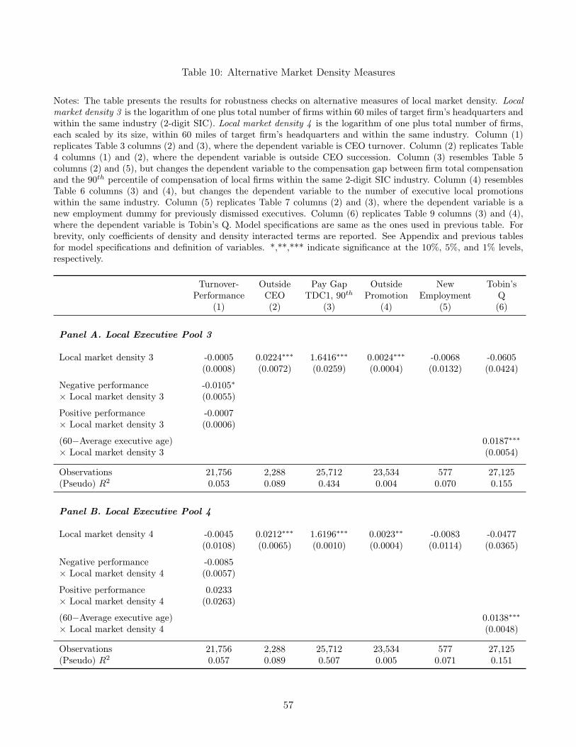
Table 10: Alternative Market Density Measures

Notes: The table presents the results for robustness checks on alternative measures of local market density. Localmarket density 3 is the logarithm of one plus total number of firms within 60 miles of target firm’s headquarters andwithin the same industry (2-digit SIC). Local market density 4 is the logarithm of one plus total number of firms,each scaled by its size, within 60 miles of target firm’s headquarters and within the same industry. Column (1)replicates Table 3 columns (2) and (3), where the dependent variable is CEO turnover. Column (2) replicates Table4 columns (1) and (2), where the dependent variable is outside CEO succession. Column (3) resembles Table 5columns (2) and (5), but changes the dependent variable to the compensation gap between firm total compensationand the 90th percentile of compensation of local firms within the same 2-digit SIC industry. Column (4) resemblesTable 6 columns (3) and (4), but changes the dependent variable to the number of executive local promotionswithin the same industry. Column (5) replicates Table 7 columns (2) and (3), where the dependent variable is anew employment dummy for previously dismissed executives. Column (6) replicates Table 9 columns (3) and (4),where the dependent variable is Tobin’s Q. Model specifications are same as the ones used in previous table. Forbrevity, only coefficients of density and density interacted terms are reported. See Appendix and previous tablesfor model specifications and definition of variables. *,**,*** indicate significance at the 10%, 5%, and 1% levels,respectively.

Turnover- Outside Pay Gap Outside New Tobin’sPerformance CEO TDC1, 90th Promotion Employment Q

(1) (2) (3) (4) (5) (6)

Panel A. Local Executive Pool 3

Local market density 3 -0.0005 0.0224∗∗∗ 1.6416∗∗∗ 0.0024∗∗∗ -0.0068 -0.0605(0.0008) (0.0072) (0.0259) (0.0004) (0.0132) (0.0424)

Negative performance -0.0105∗× Local market density 3 (0.0055)

Positive performance -0.0007× Local market density 3 (0.0006)

(60−Average executive age) 0.0187∗∗∗× Local market density 3 (0.0054)

Observations 21,756 2,288 25,712 23,534 577 27,125(Pseudo) R2 0.053 0.089 0.434 0.004 0.070 0.155

Panel B. Local Executive Pool 4

Local market density 4 -0.0045 0.0212∗∗∗ 1.6196∗∗∗ 0.0023∗∗ -0.0083 -0.0477(0.0108) (0.0065) (0.0010) (0.0004) (0.0114) (0.0365)

Negative performance -0.0085× Local market density 4 (0.0057)

Positive performance 0.0233× Local market density 4 (0.0263)

(60−Average executive age) 0.0138∗∗∗× Local market density 4 (0.0048)

Observations 21,756 2,288 25,712 23,534 577 27,125(Pseudo) R2 0.057 0.089 0.507 0.005 0.071 0.151

57