executive summary - bsi · example 1-3: 24” steel pipe – driven pile sand (api) problem...
TRANSCRIPT


2
EXECUTIVE SUMMARY
This report summarizes verification efforts dedicated to axial soil resistance modeling in
FB-MultiPier. Presented herein are quantitative comparisons between program-generated
and manually-calculated axial soil resistance curves. Included among the quantitative
comparisons are the skin (t-z) and tip (q-z) forms of resistance for all available empirical
axial resistance models in FB-MultiPier.

3
TABLE OF CONTENTS
1. Deep foundation members embedded in cohesionless soils ............................................4
2. Deep foundation members embedded in cohesive soils ................................................17
3. Deep foundation members embedded in rock ...............................................................26

4
Chapter 1
Deep foundation members embedded in
cohesionless soils
In this chapter, deep foundation soil resistance model components are compared between
FB-MultiPier and manual calculations for axially loaded piles/shafts embedded in
cohesionless soils. The following empirical models are available for generating axial (skin,
t-z; tip, q-z) load transfer curves in cohesionless soils:
1. Driven Pile (McVay)
2. Driven Pile Sand (Mosher)
3. Driven Pile Sand (API)
4. Drilled Shaft Sand
5. Drilled Shaft Gravelly Sand
6. Drilled Shaft Gravel
References:
1. McVay, M. C., O'Brien, M., Townsend, F. C., Bloomquist, D. G., and Caliendo, J.
A. (1989). "Numerical Analysis of Vertically Loaded Pile Groups," ASCE
Foundation Engineering Congress, Northwestern University, Illinois, July, pp.
675-690.
2. Mosher, R. L. (1984). Load Transfer Criteria for Numerical Analysis of Axially
Loaded Piles in Sand. Technical Report K-84-1, U. S. Army Waterways
Experiment Station, Automatic Data Processing Center, Vicksburg, Mississippi.
3. Vijayvergiya, V. N. (1977). "Load-movement characteristics of piles,"
Proceedings, Ports 77, American Society of Civil Engineers, Vol II, 269-286.
4. American Petroleum Institute (2014). Geotechincal and Foundation Design
Considerations. API RP 2 GEO 1, 1st Ed.
5. Reese, L. C., and O'Neill, M. W. (1988). Drilled Shafts: Construction Procedures
and Design Methods. Publication No. HI-88-042, Federal Highway Administration,
McLean, Virginia, 564.
6. Rollins, K. M., Clayton, R. J., Mikesell, R. C., and Blaise, B. C. (2005). "Drilled
Shaft Side Friction in Gravelly Soils." Journal of Geotechnical and
Geoenvironmental Engineering, 131(8).

5
Example 1-1: 24” Steel Pipe – Driven Pile (McVay)
Problem Description: Determine the axial load transfer curves (t-z, q-z) for a 24” steel pipe pile (0.5” thickness)
subjected to axial loading. The pile is embedded in a single layer of cohesionless soil, with use of the Driven Pile
(McVay) t-z and q-z models. The pile tip is assumed to be plugged.
24” Pipe Pile Section
File: Pipe_Pile_Driven_Pile_McVay.in
Parameter List:
γ total unit weight
G shear modulus
υ Poisson’s ratio
σnom nominal unit skin friction
Qnom nominal tip resistance
Example Summary: The computed and manually generated load transfer curves (t-z, q-
z) show agreement to within 1%.
pcf
G = 0.58 ksi
υ = 0.3
σnom = 5221 psf
P = 10 kips
56.67 ft
Driven Pile (McVay)
10 ft
P
t-z parameters
G = 2.9 ksi
υ = 0.25
Qnom = 472 kips
q-z parameters

6
Figure 1.1 Comparison of computed versus manually generated t-z curves at 24.50-ft depth
Figure 1.2 Comparison of computed versus manually generated q-z curves at pile tip
0
5
10
15
20
25
30
35
0 0.2 0.4 0.6 0.8 1 1.2 1.4
t (p
si)
z (in)
Driven Pile (McVay)
FBMP
0
20
40
60
80
100
120
140
160
180
200
0 0.5 1 1.5 2 2.5
q (
kip
s)
z (in)
Driven Pile (McVay)
FBMP

7
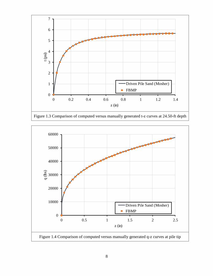
Example 1-2: 24” Steel Pipe – Driven Pile Sand (Mosher)
Problem Description: Determine the axial load transfer curves (t-z, q-z) for a 24” steel pipe pile (0.5” thickness)
subjected to axial loading. The pile is embedded in a single layer of cohesionless soil, with use of the Driven Pile
Sand (Mosher) t-z and q-z models. The pile tip is assumed to be plugged.
24” Pipe Pile Section
File: Pipe_Pile_Driven_Pile_Sand_Mosher.in
Parameter List:
γ total unit weight
σnom nominal unit skin friction
Mint initial modulus
Drel relative density exponent
∆crit critical displacement
Qnom nominal tip resistance
Example Summary: The computed and manually generated load transfer curves (t-z, q-
z) show agreement to within 1%.
pcf
σnom = 860 psf
Mint = 0.083 kci
P = 10 kips
56.67 ft
Driven Pile Sand (Mosher)
10 ft
P
t-z parameters
Drel = 0.33
∆crit = 0.25 in.
Qnom = 26 kips
q-z parameters
8
Figure 1.3 Comparison of computed versus manually generated t-z curves at 24.50-ft depth
Figure 1.4 Comparison of computed versus manually generated q-z curves at pile tip
0
1
2
3
4
5
6
7
0 0.2 0.4 0.6 0.8 1 1.2 1.4
t (p
si)
z (in)
Driven Pile Sand (Mosher)
FBMP
0
10000
20000
30000
40000
50000
60000
0 0.5 1 1.5 2 2.5
q (
lbs)
z (in)
Driven Pile Sand (Mosher)
FBMP

9
Example 1-3: 24” Steel Pipe – Driven Pile Sand (API)
Problem Description: Determine the axial load transfer curves (t-z, q-z) for a 24” steel pipe pile (0.5” thickness)
subjected to axial loading. The pile is embedded in a single layer of cohesionless soil, with use of the Driven Pile
Sand (API) t-z and q-z models. The pile tip is assumed to be unplugged.
24” Pipe Pile Section
File: Pipe_Pile_Driven_Pile_Sand_API.in
Parameter List:
γ total unit weight
ϕ internal friction angle
k coefficient of lateral earth pressure
Fnom nominal unit side friction
∆Fnom displacement at nominal unit side friction
Bnom nominal unit end bearing
Bcap bearing capacity factor
Example Summary: The computed and manually generated load transfer curves (t-z, q-
z) show agreement to within 1%.
pcf
ϕ = 35°
k =0.45
Fnom = 1691 psf
∆Fnom = 0.24 in.
P = 20 kips
56.67 ft
Driven Pile Sand (API)
10 ft
P
t-z parameters
pcf
ϕ = 32°
Bnom = 0.72 ksi
Bcap = 20
q-z parameters

10
Figure 1.5 Comparison of computed versus manually generated t-z curves at 24.50-ft depth
Figure 1.6 Comparison of computed versus manually generated q-z curves at pile tip
0
2
4
6
8
10
12
14
0 0.05 0.1 0.15 0.2 0.25 0.3 0.35 0.4
t (p
si)
z (in)
Driven Pile Sand (API)
FBMP
0
5000
10000
15000
20000
25000
30000
0 0.5 1 1.5 2 2.5
q (
lbs)
z (in)
Driven Pile Sand (API)
FBMP

11
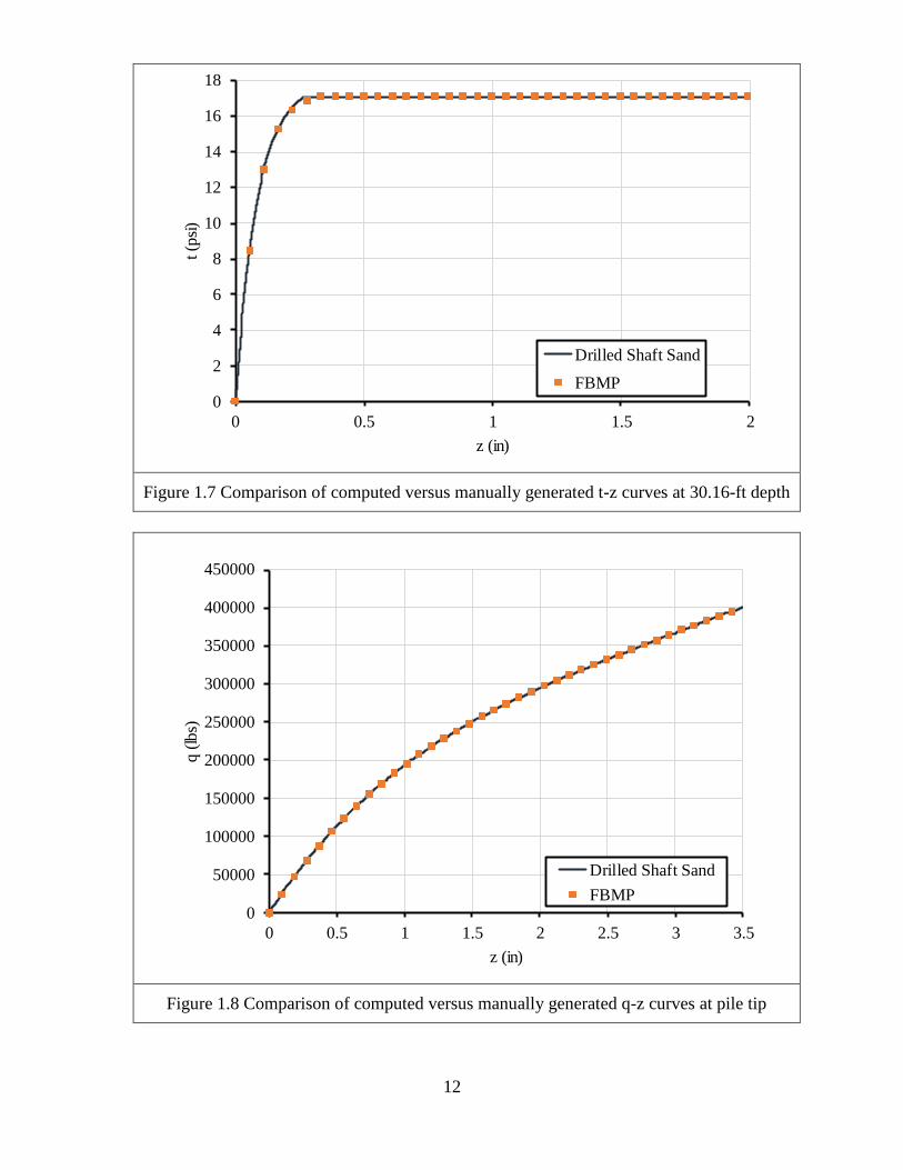
Example 1-4: 36” Reinforced Concrete Shaft – Drilled Shaft Sand
Problem Description: Determine the axial load transfer curves (t-z, q-z) for a 36” reinforced concrete shaft
subjected to axial loading. The shaft is embedded in a single layer of cohesionless soil, with use of the Drilled Shaft
Sand t-z and q-z models.
36” Concrete Shaft Section
File: Conc_Shaft_Drilled_Shaft_Sand.in
Parameter List:
γ total unit weight
N uncorrected SPT
Example Summary: The computed and manually generated load transfer curves (t-z, q-
z) show agreement to within 1%.
pcf
P = 150 kips
66.67 ft
Drilled Shaft Sand
P
t-z parameters
N = 33 blows/ft
q-z parameters
12
Figure 1.7 Comparison of computed versus manually generated t-z curves at 30.16-ft depth
Figure 1.8 Comparison of computed versus manually generated q-z curves at pile tip
0
2
4
6
8
10
12
14
16
18
0 0.5 1 1.5 2
t (p
si)
z (in)
Drilled Shaft Sand
FBMP
0
50000
100000
150000
200000
250000
300000
350000
400000
450000
0 0.5 1 1.5 2 2.5 3 3.5
q (
lbs)
z (in)
Drilled Shaft Sand
FBMP

13
Example 1-5: 36” Reinforced Concrete Shaft – Drilled Shaft Gravelly Sand
Problem Description: Determine the axial load transfer curves (t-z, q-z) for a 36” reinforced concrete shaft
subjected to axial loading. The shaft is embedded in a single layer of cohesionless soil, with use of the Drilled Shaft
Gravelly Sand t-z and q-z models.
36” Concrete Shaft Section
File: Conc_Shaft_Drilled_Gravelly_Sand.in
Parameter List:
skin friction factor
R range (1=lower, 2=average, 3=upper)
N uncorrected SPT
Example Summary: The computed and manually generated load transfer curves (t-z, q-
z) show agreement to within 1%.
= 0.25
R = 2 (Average)
P = 10 kips
66.67 ft
Drilled Shaft Gravelly Sand
P
t-z parameters
N = 33 blows/ft
q-z parameters

14
Figure 1.9 Comparison of computed versus manually generated t-z curves at 30.16-ft depth
Figure 1.10 Comparison of computed versus manually generated q-z curves at pile tip
0
1
2
3
4
5
6
0 0.5 1 1.5 2
t (p
si)
z (in)
Drilled Shaft Gravelly Sand
FBMP
0
50000
100000
150000
200000
250000
300000
350000
400000
450000
0 0.5 1 1.5 2 2.5 3 3.5
q (
lbs)
z (in)
Drilled Shaft Gravelly Sand
FBMP

15
Example 1-6: 36” Reinforced Concrete Shaft – Drilled Shaft Gravel
Problem Description: Determine the axial load transfer curves (t-z, q-z) for a 36” reinforced concrete shaft
subjected to axial loading. The shaft is embedded in a single layer of cohesionless soil, with use of the Drilled Shaft
Gravel t-z and q-z models.
36” Concrete Shaft Section
File: Conc_Shaft_Drilled_Gravel.in
Parameter List:
skin friction factor
R range (1=lower, 2=average, 3=upper)
N uncorrected SPT
Example Summary: The computed and manually generated load transfer curves (t-z, q-
z) show agreement to within 1%.
= 1.5377
R = 2 (Average)
P = 150 kips
66.67 ft
Drilled Shaft Gravel
P
t-z parameters
N = 33 blows/ft
q-z parameters

16
Figure 1.11 Comparison of computed versus manually generated t-z curves at 30.16 ft
depth
Figure 1.12 Comparison of computed versus manually generated q-z curves at pile tip
0
5
10
15
20
25
30
35
40
0 0.25 0.5 0.75 1 1.25 1.5 1.75
t (p
si)
z (in)
Drilled Shaft Gravel
FBMP
0
50000
100000
150000
200000
250000
300000
350000
400000
450000
0 0.5 1 1.5 2 2.5 3 3.5
q (
lbs)
z (in)
Drilled Shaft Gravel
FBMP

17
Chapter 2
Deep foundation members embedded in
cohesive soils
In this chapter, deep foundation soil resistance model components are compared between
FB-MultiPier and manual calculations for axially loaded piles/shafts embedded in cohesive
soils. The following empirical models are available for generating axial (skin, t-z; tip, q-z)
load transfer curves in cohesive soils:
1. Driven Pile Clay (Skempton)
2. Driven Pile Clay (API)
3. Drilled Shaft Clay
4. Drilled Shaft Clay-Shale
References:
1. Skempton, A. W. (1951). "The Bearing Capacity of Clays." Proceedings, Building
Research Congress, Vol I, Part IIV, 180-189.
2. American Petroleum Institute (2014). Geotechincal and Foundation Design
Considerations. API RP 2 GEO 1, 1st Ed.
3. Reese, L. C., and O'Neill, M. W. (1988). Drilled Shafts: Construction Procedures
and Design Methods. Publication No. HI-88-042, Federal Highway Administration,
McLean, Virginia, 564.
4. Wang, S. T., and Reese, L. C., (1993) COM624P – Laterally loaded pile analysis
for the microcomputer, ver. 2.0. FHWA-SA-91-048, Springfield, VA.
5. Aurora, R., and Reese, L. C. (1977). "Field Tests of Drilled Shafts in Clay-Shales."
Ninth International Conference on Soil Mechanics and Foundation Engineering,
Tokyo, Japan, 371-376.

18
Example 2-1: 24” Steel Pipe – Driven Pile Clay (Skempton)
Problem Description: Determine the axial load transfer curves (t-z, q-z) for a 24” steel pipe pile (0.5” thickness)
subjected to axial loading. The pile is embedded in a single layer of cohesive soil, with use of the Driven Pile Clay
(Skempton) t-z and q-z models. The pile tip is assumed to be plugged.
24” Pipe Pile Section
File: Pipe_Pile_Driven_Pile_Clay_Skempton.in
Parameter List:
γ total unit weight
σnom nominal unit skin friction
Cu undrained shear strength
e50 major principal strain @ 50
∆exp displacement exponent
Example Summary: The computed and manually generated load transfer curves (t-z, q-
z) show agreement to within 1%.
pcf
σnom = 1440 psf
P = 10 kips
56.67 ft
Driven Pile Clay (Skempton)
10 ft
P
t-z parameters
Cu = 1044.2 psf
e50 = 0.01
∆exp = 0.5
q-z parameters

19
Figure 2.1 Comparison of computed versus manually generated t-z curves at 24.50-ft depth
Figure 2.2 Comparison of computed versus manually generated q-z curves at pile tip
0
2
4
6
8
10
12
0 0.05 0.1 0.15 0.2
t (p
si)
z (in)
Driven Pile Clay (Skempton)
FBMP
0
5000
10000
15000
20000
25000
30000
35000
40000
0 0.5 1 1.5 2 2.5 3
q (
lbs)
z (in)
Driven Pile Clay (Skempton)
FBMP

20
Example 2-2: 24” Steel Pipe – Driven Pile Clay (API)
Problem Description: Determine the axial load transfer curves (t-z, q-z) for a 24” steel pipe pile (0.5” thickness)
subjected to axial loading. The pile is embedded in a single layer of cohesive soil, with use of the Driven Pile Clay
(API) t-z and q-z models. The pile tip is assumed to be unplugged.
24” Pipe Pile Section
File: Pipe_Pile_Driven_Pile_Clay_API.in
Parameter List:
γ total unit weight
Cu undrained shear strength
Example Summary: The computed and manually generated load transfer curves (t-z, q-
z) show agreement to within 1%.
pcf
Cu = 2088.5 psf
P = 10 kips
56.67 ft
Driven Pile Clay (API)
10 ft
P
t-z parameters
pcf
Cu = 1044.2 psf
q-z parameters

21
Figure 2.3 Comparison of computed versus manually generated t-z curves at 24.50-ft depth
Figure 2.4 Comparison of computed versus manually generated q-z curves at pile tip
0
1
2
3
4
5
6
7
8
9
10
0 0.25 0.5 0.75 1 1.25
t (p
si)
z (in)
Driven Pile Clay (API)
FBMP
0
1000
2000
3000
4000
5000
6000
0 1 2 3 4
q (
lbs)
z (in)
Driven Pile Clay (API)
FBMP

22
Example 2-3: 36” Reinforced Concrete Shaft – Drilled Shaft Clay
Problem Description: Determine the axial load transfer curves (t-z, q-z) for a 36” reinforced concrete shaft
subjected to axial loading. The shaft is embedded in a single layer of cohesive soil, with use of the Drilled Shaft
Clay t-z and q-z models.
36” Concrete Shaft Section
File: Conc_Shaft_Drilled_Clay.in
Parameter List:
γ total unit weight
Cu undrained shear strength
Example Summary: The computed and manually generated load transfer curves (t-z, q-
z) show agreement to within 1%.
pcf
Cu = 3000 psf
P = 150 kips
66.67 ft
Drilled Shaft Clay
P
t-z parameters
Cu = 3000 psf
q-z parameters

23
Figure 2.5 Comparison of computed versus manually generated t-z curves at 30.16-ft depth
Figure 2.6 Comparison of computed versus manually generated q-z curves at pile tip
0
2
4
6
8
10
12
0 0.5 1 1.5 2
t (p
si)
z (in)
Drilled Shaft Clay
FBMP
0
20000
40000
60000
80000
100000
120000
140000
160000
180000
200000
0 0.5 1 1.5 2 2.5 3 3.5
q (
lbs)
z (in)
Drilled Shaft Clay
FBMP

24
Example 2-4: 36” Reinforced Concrete Shaft – Drilled Shaft Clay-Shale
Problem Description: Determine the axial load transfer curves (t-z, q-z) for a 36” reinforced concrete shaft
subjected to axial loading. The shaft is embedded in a single layer of cohesive soil, with use of the Drilled Shaft
Clay-Shale t-z and q-z models.
36” Concrete Shaft Section
File: Conc_Shaft_Drilled_Clay-Shale.in
Parameter List:
γ total unit weight
Cu undrained shear strength
skin friction factor (alpha)
Bcap bearing capacity factor
Example Summary: The computed and manually generated load transfer curves (t-z, q-
z) show agreement to within 1%.
pcf
Cu = 754 psf
= 0.75
P = 100 kips
66.67 ft
Drilled Shaft Clay-Shale
P
t-z parameters
Cu = 754 psf
Bcap = 8
q-z parameters

25
Figure 2.7 Comparison of computed versus manually generated t-z curves at 30.16-ft depth
Figure 2.8 Comparison of computed versus manually generated q-z curves at pile tip
0
0.5
1
1.5
2
2.5
3
3.5
4
4.5
0 0.5 1 1.5 2
t (p
si)
z (in)
Drilled Shaft Clay-Shale
FBMP
0
5000
10000
15000
20000
25000
30000
35000
40000
45000
0 0.5 1 1.5 2 2.5 3 3.5
q (
lbs)
z (in)
Drilled Shaft Clay-Shale
FBMP

26
Chapter 3
Deep foundation members embedded in rock
In this chapter, deep foundation soil resistance model components are compared between
FB-MultiPier and manual calculations for axially loaded piles/shafts embedded in rock.
The following empirical models are available for generating axial (skin, t-z; tip, q-z) load
transfer curves in rock:
1. Drilled Shaft IGM (Cohesive)
2. Drilled Shaft IGM (Non-Cohesive)
3. Drilled Shaft Limestone (McVay)*
* t-z model only
References:
1. O’Neill, M. W., Townsend, F. C., Hassan, K. M., Buller, A., and Chan, P. S. (1996).
Load Transfer for Drilled Shafts in Intermediate Geomaterials. FHWA-RD-95-
172.
2. Mayne, P. W., Harris, D. E. (1993). Axial Load-Displacement Behavior of Drilled
Shaft Foundations in Piedmont Residium. FHWA-RD41-30-2175.
3. McVay, M. C., M., Niraula, L., (2004). Development of Modified T-Z Curves for
Large Diameter Piles/Drilled Shafts in Limestone for FB-Pier. Florida Department
of Transportation, 4910-4504-878-12, National Technical Information Service,
Springfield, VA.

27
Example 3-1: 36” Reinforced Concrete Shaft – Drilled Shaft IGM (Cohesive)
Problem Description: Determine the axial load transfer curves (t-z, q-z) for a 36” reinforced concrete shaft
subjected to axial loading. The pile is embedded in a single layer of cohesive soil, with use of the Drilled Shaft
IGM (Cohesive) t-z and q-z models.
36” Concrete Shaft Section
File: Conc_Shaft_Drilled_IGM_Cohesive.in
Parameter List:
γ total unit weight
qu unconfined compressive strength
m mass modulus
Em/i modulus ratio
Sur surface (1=rough, 2=smooth)
Ts split tensile strength
γsc unit weight shaft concrete
SL slump
IGMm IGM mass modulus
Example Summary: The computed and manually generated load transfer curves (t-z, q-
z) show agreement to within 1%.
pcf
qupsf
Em = 40.03 ksi
Em/I = 1
Ts = 50125 psf
γsc = 131.03 pcf
SL = 4.92 in.
P = 100 kips
66.67 ft
Drilled Shaft IGM (Cohesive)
P
t-z parameters
IGMm = 40 ksi
q-z parameters

28
Figure 3.1 Comparison of computed versus manually generated t-z curves at 30.16 ft-depth
Figure 3.2 Comparison of computed versus manually generated q-z curves at pile tip
0
20
40
60
80
100
120
140
0 0.5 1 1.5 2
t (p
si)
z (in)
Drilled Shaft IGM Cohesive
FBMP
0
100000
200000
300000
400000
500000
600000
700000
800000
0 0.5 1 1.5 2 2.5 3 3.5
q (
lbs)
z (in)
Drilled Shaft IGM Cohesive
FBMP

29
Example 3-2: 36” Reinforced Concrete Shaft – Drilled Shaft IGM (Non-Cohesive)
Problem Description: Determine the axial load transfer curves (t-z, q-z) for a 36” reinforced concrete shaft
subjected to axial loading. The pile is embedded in a single layer of cohesive soil, with use of the Drilled Shaft
IGM (Non-Cohesive) t-z and q-z models.
36” Concrete Shaft Section
File: Conc_Shaft_Drilled_IGM_Non-Cohesive.in
Parameter List:
γ total unit weight
N60 SPT Blow Count
υ Poisson’s ratio
SD socket diameter
Example Summary: The computed and manually generated load transfer curves (t-z, q-
z) show agreement to within 1%.
pcf
N60 = 100 blows/ft
= 0.4
SD = 36 in.
P = 100 kips
66.67 ft
Drilled Shaft IGM (Non-Cohesive)
P
t-z parameters
pcf
N60 = 100 blows/ft
= 0.4
SD = 36 in.
q-z parameters

30
Figure 3.3 Comparison of computed versus manually generated t-z curves at 30.16-ft depth
Figure 3.4 Comparison of computed versus manually generated q-z curves at pile tip
0
5
10
15
20
25
30
35
40
45
0 0.5 1 1.5 2
t (p
si)
z (in)
Drilled Shaft IGM Non-Cohesive
FBMP
0
50000
100000
150000
200000
250000
300000
350000
0 0.2 0.4 0.6 0.8 1 1.2
q (
lbs)
z (in)
Drilled Shaft IGM Non-Cohesive
FBMP

31
Example 3-3: 36” Reinforced Concrete Shaft – Drilled Shaft Limestone (McVay)
Problem Description: Determine the axial load transfer curve (t-z) for a 36” reinforced concrete shaft subjected
to axial loading. The pile is embedded in a single layer of cohesive soil, with use of the Drilled Shaft Limestone
(McVay) t-z model.
36” Concrete Shaft Section
File: Conc_Shaft_Drilled_Limestone_McVay.in
Parameter List:
σnom nominal unit skin friction
Example Summary: The computed and manually generated load transfer curves (t-z)
show agreement to within 1%.
σnom = 41770 psf
P = 100 kips
66.67 ft
Drilled Shaft Limestone (McVay)
P
t-z parameters

32
Figure 3.5 Comparison of computed versus manually generated t-z curves at 30.16-ft depth
0
50
100
150
200
250
300
350
0 0.5 1 1.5 2
t (p
si)
z (in)
Drilled Shaft Limestone Mcvay
FBMP

33
ACKNOWLEDGEMENT
This report was developed by BSI engineers and researchers, including, but not limited to:
Amirata Taghavi, Brandon Lypher, and Michael Davidson.