executive summary - odfw home page department of fish and wildlife – attachment 2: biological...
TRANSCRIPT

Oregon Department of Fish and Wildlife – Attachment 2: Biological Status Review for Gray Wolf
1
Attachment 2
Oregon Department of Fish and Wildlife
(March 31, 2015)
Biological status review for the Gray Wolf (Canis lupus) in Oregon and evaluation of
criteria to remove the Gray Wolf from the List of Endangered Species under the Oregon
Endangered Species Act
Executive Summary
Oregon wolves are listed as an endangered species under the Oregon Endangered Species Act
(OESA). The Oregon Wolf Conservation and Management Plan (hereafter Wolf Plan) contains a
conservation population objective predicted to support the requirements for delisting the species
under OESA. The conservation objective was achieved in January 2015 and this draft document
is prepared to present information to the Oregon Fish and Wildlife Commission (Commission)
on the biological status of gray wolves in Oregon.
Through natural dispersal from neighboring Idaho, wolves became established in Oregon in 2008
and have increased in both distribution and abundance during all years. At the end of 2014 there
was a minimum of 77 known wolves in 15 groups within Oregon. This included 9 packs and 8 of
those packs were successful breeding pairs in 2014. Our analysis as part of this biological review
predicts that Oregon’s wolf population will continue to increase.
Delisting a species from Oregon ESA (ORS 496.176) requires a public rulemaking and findings
decision by the Commission and these decisions are to be made on the basis of scientific
information and other biological data. Specifically, the Commission must evaluate the biological
status of the species and determine if:
1. The species is not now (and is not likely in the foreseeable future to be) in danger of
extinction in any significant portion of its range in Oregon or in danger of becoming
endangered; and
2. The species’ natural reproductive potential is not in danger of failure due to limited
population numbers, disease, predation, or other natural or human-related factors
affecting its continued existence; and
3. Most populations are not undergoing imminent or active deterioration of range or primary
habitat; and
4. Over-utilization of the species or its habitat for commercial, recreational, scientific, or
educational purposes is not occurring or likely to occur; and
5. Existing state or federal programs or regulations are adequate to protect the species and
its habitat.
This draft biological status review contains information related to each of these criteria. A
significant portion of the analysis (Criterion 1 & 2) is included as separate draft reports in
Appendix’s A & B of this document.

Oregon Department of Fish and Wildlife – Attachment 2: Biological Status Review for Gray Wolf
2
Introduction
Historical accounts show that prior to extirpation from Oregon and other western states gray
wolves (Canis lupus) were widely distributed and efforts by early Euro-American immigrants
were largely directed at eliminating the predator (Oregon Department of Fish and Wildlife
2010). This effort was successful and wolves were extirpated from most of the western United
States by the mid-twentieth century. Conversely, modern recovery efforts in the Northern Rocky
Mountains and subsequent conservation actions in the western United States led to restored gray
wolf populations throughout a portion of its historical range.
In 1995 and 1996, the United States Fish and Wildlife Service (USFWS) reintroduced 66 gray
wolves into the Rocky Mountains of Idaho and Wyoming. The reintroductions and associated
conservation measures were part of the 1987 Northern Rocky Mountain (NRM) Wolf Recovery
Plan and were responsible for the successful reestablishment of wolves in Wyoming, Idaho,
Montana, and later in parts of Oregon and Washington. In 2013, the NRM wolf population was
estimated at 1,691 (U. S. Fish and Wildlife Service et al. 2014).
Though gray wolves were not reintroduced into Oregon, wolf experts predicted wolves from a
successful NRM population – especially Idaho – would eventually travel to and colonize Oregon.
This prediction was soon realized and between 1999 and 2007, at least 4 individual wolves were
documented to have dispersed into Oregon from Idaho. In July 2008, Oregon Department of Fish
and Wildlife (ODFW) biologists discovered a wolf pack with pups in the Wenaha River area of
northeastern Oregon which was the first documented reproductive event since wolves were
extirpated from Oregon. The Oregon wolf population has steadily increased and in 2014 ODFW
documented a minimum known population of 77 wolves distributed across 15 pairs and packs.
State and Federal Regulatory Status and Actions in Oregon
Wolves were classified as endangered in Oregon in 1987 when the Oregon Endangered Species
Act (OESA) was enacted. The OESA requires the conservation of listed species and generally
defines conservation as the use of methods and procedures necessary to bring a species to the
point at which the measures provided are no longer necessary. To achieve this mandate, the
Oregon Fish and Wildlife Commission (Commission) exercised its authority under the OESA by
adopting and implementing the Oregon Wolf Conservation and Management Plan (Wolf Plan) in
2005. The Wolf Plan requires reevaluation every five years and was last updated in 2010.
In the early stages of implementation, the Wolf Plan focused on methods and procedures to
conserve wolves so that the species is self-sustaining and can be delisted. The Wolf Plan defined
a population objective of four breeding pairs of wolves for three consecutive years in eastern
Oregon as the guideline for when wolves may be considered for statewide delisting from OESA.
Accordingly, the Wolf Plan was drafted to meet the five delisting criteria identified in Oregon
Revised Statute (ORS) 496.176 and Oregon Administrative Rule (OAR) 635-100-0112.
In 1987, the USFWS completed the NRM Wolf Recovery Plan. Four years later Congress
initiated an administrative process to reintroduce wolves into Yellowstone National Park and
central Idaho. Extensive public input showed general support for wolf recovery, and the U.S.
Secretary of Interior approved reintroduction. In 1995 and 1996, 66 wolves were captured in
Alberta and British Columbia, Canada. Of those, 35 were released in central Idaho and 31 were
released into Yellowstone National Park.

Oregon Department of Fish and Wildlife – Attachment 2: Biological Status Review for Gray Wolf
3
At the time Oregon’s Wolf Plan was first adopted in 2005, wolves were listed as endangered
under the federal Endangered Species Act (ESA). To emphasize close coordination between the
U.S. Fish and Wildlife Service (USFWS) and ODFW, the 2007 Federal/State Coordination
Strategy for Implementation of Oregon’s Wolf Plan was developed which outlined procedures
for managing wolves while they remained federally listed. In 2007, the USFWS proposed to
designate the NRM gray wolf population as a distinct population segment and remove their
status as endangered under federal ESA. The resulting decision to delist (and subsequent
delisting decisions) was met with litigation and between 2008 and 2011 the status of NRM
wolves varied between listed and delisted. In May 2011, NRM wolves, which included areas
east of Highways 395-78-95 in Oregon, were delisted as a result of congressional action.
Wolves in the remainder of Oregon remained listed as endangered under federal ESA (Figure 1).
Figure 1. Current Federal ESA Status of Wolves in Oregon
Oregon Department of Fish and Wildlife – Attachment 2: Biological Status Review for Gray Wolf
4
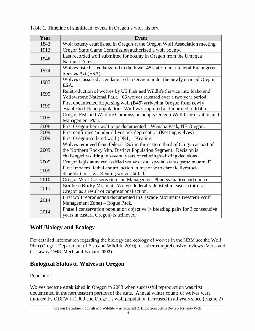
Table 1. Timeline of significant events in Oregon’s wolf history.
Year Event
1843 Wolf bounty established in Oregon at the Oregon Wolf Association meeting.
1913 Oregon State Game Commission authorized a wolf bounty.
1946 Last recorded wolf submitted for bounty in Oregon from the Umpqua
National Forest.
1974 Wolves listed as endangered in the lower 48 states under federal Endangered
Species Act (ESA).
1987 Wolves classified as endangered in Oregon under the newly enacted Oregon
ESA.
1995 Reintroduction of wolves by US Fish and Wildlife Service into Idaho and
Yellowstone National Park. 66 wolves released over a two year period.
1999 First documented dispersing wolf (B45) arrived in Oregon from newly
established Idaho population. Wolf was captured and returned to Idaho.
2005 Oregon Fish and Wildlife Commission adopts Oregon Wolf Conservation and
Management Plan.
2008 First Oregon-born wolf pups documented – Wenaha Pack, NE Oregon.
2009 First confirmed ‘modern’ livestock depredation (Keating wolves).
2009 First Oregon-collared wolf (OR1) – Keating.
2009
Wolves removed from federal ESA in the eastern third of Oregon as part of
the Northern Rocky Mtn. Distinct Population Segment. Decision is
challenged resulting in several years of relisting/delisting decisions.
2009 Oregon legislature reclassified wolves as a “special status game mammal”.
2009 First ‘modern’ lethal control action in response to chronic livestock
depredation – two Keating wolves killed.
2010 Oregon Wolf Conservation and Management Plan evaluation and update.
2011 Northern Rocky Mountain Wolves federally delisted in eastern third of
Oregon as a result of congressional action.
2014 First wolf reproduction documented in Cascade Mountains (western Wolf
Management Zone) – Rogue Pack.
2014 Phase I conservation population objective (4 breeding pairs for 3 consecutive
years in eastern Oregon) is achieved.
Wolf Biology and Ecology
For detailed information regarding the biology and ecology of wolves in the NRM see the Wolf
Plan (Oregon Department of Fish and Wildlife 2010), or other comprehensive reviews (Verts and
Carraway 1998, Mech and Boitani 2003).
Biological Status of Wolves in Oregon
Population
Wolves became established in Oregon in 2008 when successful reproduction was first
documented in the northeastern portion of the state. Annual winter counts of wolves were
initiated by ODFW in 2009 and Oregon’s wolf population increased in all years since (Figure 2)

Oregon Department of Fish and Wildlife – Attachment 2: Biological Status Review for Gray Wolf
5
with a mean population growth rate of 1.41 (± .17SD). At the end of 2014, a minimum of 77
wolves occurred in Oregon (Oregon Department of Fish and Wildlife 2015). This included 9
packs, defined as four or more wolves travelling together in winter (Oregon Department of Fish
and Wildlife 2010). In addition, 6 new groups of wolves were documented in January 2015, and
of these, 5 are known to be male-female pairs (Table 2). Oregon uses a minimum-observed
count method for surveying wolves which likely underestimates the actual population because it
is unrealistic to assume perfect detection of all wolves. Furthermore, survey effort is directed at
known groups or packs and does not account for individual or non-territorial wolves which are
known to occur in all wolf populations.
Figure 2. Oregon minimum wolf population 2009-2014.
Table 2. Population summary data for Oregon. Shaded cells denote successful breeding pairs.
Pack/Area 2009 2010 2011 2012 2013 2014
Imnaha Pack 10 15 5 8 6 5
Wenaha Pack 4 6 5 11 9 11
Walla Walla Pack 8 6 9 9
Snake River Pack 5 7 9 6
Umatilla River Pack 2 4 6 8
Minam Pack 7 12 9
Mt Emily Pack 4 7
Meacham Pack 5
Rogue Pack 5
Catherine Cr / Keating Units Pack 5 0
Desolation Pair 2
Chesnimnus Pair 2
Catherine Pair 2
Sled Springs Pair 2 2
South Snake Wolves 2
Keno Pair 2
Individual wolves 4 3 4 0
Minimum Total 14 21 29 48 64 77
0
10
20
30
40
50
60
70
80
90
2009 2010 2011 2012 2013 2014

Oregon Department of Fish and Wildlife – Attachment 2: Biological Status Review for Gray Wolf
6
Reproduction and Pup Survival
Minimum number of breeding pairs in Oregon increased since 2009 but annual variation was
present (Figure 2). Breeding pairs are considered successful if at least 2 pups survive and are
documented at the end of the calendar year. In 2014, 7 of 8 Oregon breeding pairs occurred
within the eastern wolf management zone (WMZ) and this marks the third consecutive year in
which at least 4 breeding pairs occurred in eastern Oregon; prompting entry into Phase II of the
Wolf Plan. Oregon’s minimum pup counts across all years indicate a pup survival rate of 0.61
(95% CI = 0.53 - 0.69) assuming 5 pups were born per litter. This is slightly lower survival, but
within the range of values reported in literature (Appendix B). Oregon’s minimum-observed
count method is likely to underestimate pup survival because pups are not always together, nor
are they always detected during winter surveys. See Appendix B for additional discussion of
reproduction and survival rates of Oregon’s wolves.
Figure 3. Successful breeding pairs of wolves in Oregon 2009-2014.
ODFW does not routinely conduct den or rendezvous surveys in all packs/years, and relies on
winter pup recruitment data to assess reproductive success. Factors affecting early pup survival
in Oregon are undetermined, though canine parvovirus was responsible for the loss of pups in the
Wenaha Pack in 2013 and illegal take was responsible for the loss of one pup of the Umatilla
River Pack in 2013.
Distribution
Since establishment in 2008, area occupied by Oregon’s wolves has expanded rapidly and
wolves currently occupy 12,582 km2. Most wolves occur within the northeastern portion of the
state, and two areas of known wolf activity occur within the southern Oregon Cascade
Mountains (Figure 4).
0
1
2
3
4
5
6
7
8
9
10
2009 2010 2011 2012 2013 2014
Packs Breeding Pairs

Oregon Department of Fish and Wildlife – Attachment 2: Biological Status Review for Gray Wolf
7
Figure 4. Current distribution of known wolves in Oregon
Dispersal
To date, ODFW has documented dispersal of 16 collared wolves from their natal territories.
Half (n=8) of the dispersals terminated within Oregon and half (n=8) emigrated from Oregon.
The observed rate of emigration was expected given proximity of wolves in northeastern Oregon
to Idaho and Washington. As Oregon’s wolf population becomes more ‘interior’ the proportion
of dispersers that emigrate is expected to decline. See Appendix B for more discussion on
dispersal and emigration. Some dispersals are ongoing, but of completed dispersals analyzed
(n=10), mean dispersal distance was 145 km2.
Figure 5. Map of Oregon-collared wolf dispersers 2009-2015

Oregon Department of Fish and Wildlife – Attachment 2: Biological Status Review for Gray Wolf
8
Habitat Use and Land Ownership.
Wolves can occupy a variety of land cover types provided adequate prey exists (Keith 1983,
Fuller 1989, Haight et al. 1998) and human activity is minimal (Oakleaf et al. 2006, Belongie
2008). GPS location data indicated wolves in Oregon primarily use forested habitat with seasonal
shifts to more open habitats that reflect seasonal distributions of prey (e.g., lower elevation elk
wintering areas). Location data from wolves collared in Oregon from 2006 to 2014 showed that
62% of all locations occurred on public and 38% on private lands (ODFW unpublished data).
Denning also occurs on both public and private land in Oregon and all known den sites occurred
within forested habitat. In 2014, 6 (67%) den sites were on National Forest lands and 3 (33%)
were on private lands.
Wolf Prey
Across their range in North America, wolves depend on native large ungulates as a primary prey
source (Haight et al. 1998, Fuller et al. 2003). Oregon is a multi-prey system with abundant elk
(Cervus elaphus), mule deer (Odocoileus hemionus), black-tailed deer (O.h. columbianus) and
white-tailed deer (Odocoileus virginianus). Though prey selection may vary in multi-prey
systems, diets of wolves in the NRM are dominated by elk wherever the two species co-occur
(Smith et al. 2004, Oakleaf et al. 2006).
Analysis of prey selection and kill rates by wolves in Oregon has not been completed, but
anecdotal observations in the northeastern Oregon indicated that elk are commonly killed by
wolves. Oregon maintains a robust and widely distributed elk population numbering an estimated
128,000 elk across 151,500 km2
(ODFW data). Between 2009 and 2014, all Wildlife
Management Units (WMU’s) of northeastern Oregon with established wolf packs for at least
four years (Imnaha, Snake River, Walla Walla, Wenaha ) had increasing elk populations, and
two of the four (Imnaha and Snake River) were above the established management objectives for
elk since wolves became established (ODFW data).
Other important wolf prey species include mule deer – estimated at 229,000 in eastern Oregon
(ODFW data), black-tailed deer (western Oregon) and white-tailed deer (esp. northeastern
Oregon). ODFW does not maintain specific population estimates of black-tailed and white-tailed
deer, though based on hunter harvest data, both species are abundant within their respective
habitats. Deer distribution overlaps with all elk range in Oregon.
Diseases and Mortality of Wolves
As with most North American wildlife populations, a variety of diseases and parasites may affect
wild wolf populations (Brand et al. 1995, Wobeser 2002). A thorough discussion of diseases
potentially affecting wolves in Oregon is contained in the Wolf Plan (Oregon Department of Fish
and Wildlife 2010).
To better understand potential exposure to several common canine diseases such as leptospirosis,
canine adenovirus, canine distemper virus, and canine parvovirus, ODFW analyzed blood serum
samples collected from captured wolves (n=19) between 2010 and 2013 within the Imnaha,
Minam, Snake River, Umatilla River, Walla Walla and Wenaha packs (Oregon Department of
Fish and Wildlife 2014). Positive parvovirus titers were found in all but 2 samples (both 4
month-old pups) and in all 6 of the packs tested. Parvovirus caused 2 instances of mortality in the

Oregon Department of Fish and Wildlife – Attachment 2: Biological Status Review for Gray Wolf
9
Wenaha pack in 2013 and was assigned as primary cause of the reproductive failure during that
year. However, the pack is still extant and was classified as a breeding pair in 2014 indicating
transient effects of parvovirus.
Distemper virus has not been detected in the Oregon wolf population but is present throughout
the state in both domestic dogs and wild canids (i.e., coyotes [Canis latrans] and foxes [Vulpes
vulpes and Urocyon cineroargenteus]) and raccoons (Procyon lotor). Though distemper
outbreaks have been documented in wolves in other states, it has not been a major source of
mortality (Brand et al. 1995). Leptospirosis titers were also detected in 2 samples from 2
different packs and canine adenovirus titers were detected in 68% of the samples from 5 different
packs (Oregon Department of Fish and Wildlife 2014).
Two important parasites in wolves are sarcoptic mange and dog-biting lice (Trichodectes canis).
Sacrcoptic mange is a contagious skin disease caused by a mite (Sarcoptes scabeii) causing
irritation and hair loss. It can lead to secondary infection and mortality of wolves (Kreeger 2003)
and has been documented in NRM wolves (Jimenez et al. 2010). However, to date, mange has
not been observed or suspected in Oregon wolves. Dog-biting lice can also cause hair loss and
stress to wolves which may lead to reduced survival (Brand et al. 1995). Examination of more
than 35 Oregon wolves and wolf carcasses between 2009 and 2015 resulted in few ectoparasites
documented. Dog-biting lice were observed in one instance in 2015 on a captured wolf of the
Imnaha pack, and though some hair loss was observed body condition was generally good.
Wolves are highly susceptible to human-caused mortality – evidenced by the widely accepted
view that human-caused eradication efforts were largely responsible for the wolf’s disappearance
throughout most of the contiguous United States. In Oregon, human-caused mortality including
illegal take (n=5), ODFW control action (n=4), vehicle collisions (n=1), and ODFW capture-
related complications (n=1) accounted for 85% of the documented wolf deaths between 2000 and
2014. Wolves are especially vulnerable to human-caused mortality in open habitats (Bangs et al.
2004) and since 2000, 82% (n=9) of the documented human-caused mortalities in Oregon
occurred within or were associated with, open habitats. This does not imply that mortality
occurred as a result of wolves utilizing open areas, but rather asserts that wolves in open habitats
are likely more susceptible to control actions, management activities which may result in death,
and illegal take. See Appendix B for additional discussion of the effects of anthropogenic
(human-caused) mortality on wolves in Oregon.
OESA Delisting Requirements and Analysis of Oregon Delisting Criteria
The Wolf Plan directed wolf management activities in Oregon to achieve the conservation
population objective of four breeding pairs of wolves for three consecutive years, and that once
this objective was reached the process to consider removing the species from the list of
endangered species under the OESA would be initiated. The conservation population objective
was based on the prediction that, if the protections of the OESA cease when the objective is met,
a naturally self-sustaining population of wolves would continue to exist in Oregon and this
population level would support the necessary findings to justify a Commission decision to delist
the species.
Oregon Revised Statute (ORS) 496.004 and Oregon Administrative Rules (OAR) 635-100-0100
defines an endangered species as “any native wildlife species determined by the Commission to
be in danger of extinction throughout any significant portion of its range within this state”.

Oregon Department of Fish and Wildlife – Attachment 2: Biological Status Review for Gray Wolf
10
OAR 635-100-0100 to 635-100-0112 guide the Commission’s procedures and criteria for listing,
delisting, and reclassifying from the list of Oregon endangered species. Furthermore, delisting a
species from OESA (ORS 496.176) requires a public rulemaking decision by the Commission
and this decision is to be made on the basis of scientific information and biological data. The
scientific information must be documented and verifiable information related to the species’
biological status.
To delist wolves in Oregon, the Commission must evaluate the biological status of the species
and determine if:
1. The species is not now (and is not likely in the foreseeable future to be) in danger of
extinction in any significant portion of its range in Oregon or in danger of becoming
endangered; and
2. The species’ natural reproductive potential is not in danger of failure due to limited
population numbers, disease, predation, or other natural or human-related factors
affecting its continued existence; and
3. Most populations are not undergoing imminent or active deterioration of range or primary
habitat; and
4. Over-utilization of the species or its habitat for commercial, recreational, scientific, or
educational purposes is not occurring or likely to occur; and
5. Existing state or federal programs or regulations are adequate to protect the species and
its habitat.
For any determination of Criterion 1 above regarding the range of a species, OAR 635-100-0105
specifies three evaluation factors to be used by the Commission:
1. The total geographic area in this state used by the species for breeding, resting, or
foraging and the portion thereof in which the species is or is likely within the foreseeable
future to become in danger of extinction; and
2. The nature of the species’ habitat, including any unique or distinctive characteristics of
the habitat the species uses for breeding, resting, or foraging; and
3. The extent to which the species habitually uses the geographic area
The following review examines the biological status of Oregon’s wolf population by analyzing
each of the five criteria above.
Criterion 1: The species is not now (and is not likely in the foreseeable future
to be) in danger of extinction throughout any significant portion of its range in
Oregon or is not at risk of becoming endangered throughout any significant
portion of its range in Oregon.
Within broadly defined habitat requirements described in this document, wolves are not
generally known to require specific or niche habitat features within areas of use. We define and
use ‘potential range’ as geographic areas of Oregon with sufficient habitat features to allow
breeding, resting, and foraging requirements of wolves per OAR 635-100-0105. It does not
include areas of contracted historical range (described below), nor does it provide a qualitative

Oregon Department of Fish and Wildlife – Attachment 2: Biological Status Review for Gray Wolf
11
assessment future wolf numbers or carrying capacity based on available habitat. A report
describing methods used for evaluating contracted historical and potential range is available in
Appendix A of this document.
Historical Range
Assessment of the baseline historical range of wolves in Oregon is difficult because: 1) historical
accounts are inconsistent and often anecdotal; and 2) human-caused effects which resulted in the
wolf’s extirpation pre-dated accurate surveys of the species. Historical accounts generally
describe a wide distribution and variable abundance within the state (Oregon Department of Fish
and Wildlife 2010), but no comprehensive surveys of wolf distribution and abundance were
conducted during this period. Scientists described wolves as occurring in both eastern (Young
1946) and western Oregon (Bailey 1936). Bounty records up to 1946 corroborated presence of
wolves from both sides of the Oregon Cascade Mountains (Olterman and Verts 1972). For this
criterion, and to facilitate our analysis, we concluded that prior to European settlement; most of
the land area within Oregon was historical wolf range.
Historical range, however, does not mean that all geographic areas of Oregon supported
sustainable sub-populations of wolves or that densities were uniformly distributed across the
state. Based on preferred cover types and our current understanding of wolf ecology, some
portions of Oregon historically contained areas of marginal or less suitable habitat. By example,
arid and non-forested areas with low prey densities would have been expected to support few
wolves (Young and Goldman 1944). In Oregon, these areas likely included much of the
Columbia Basin and Great Basin rangeland habitats.
Contraction of Historical Range in Oregon
Human activities affect wolf distribution (Mladenoff et al. 1995) and the absence of wolves in
human-dominated areas may reflect high anthropogenic mortality, avoidance, or both (Mech and
Boitani 2003). We used human density, road density, and cultivated agriculture areas to identify
geographic areas that would be unsuitable for wolf establishment. We estimated permanent
contraction of historical range of at least 60,746 km2
(24%) of Oregon has occurred to date
(Figure 6). A large proportion of which occurs in the Willamette Valley, where dense human
population, cultivated landscape, lack of forest cover and high road density is expected to
preclude significant reestablishment of resident wolves under any protection level or
management policy.

Oregon Department of Fish and Wildlife – Attachment 2: Biological Status Review for Gray Wolf
12
Figure 6. Estimated areas of contracted wolf range in Oregon.
Potential Range
Several studies have assessed habitat features as related to occupancy and persistence of wolves,
and though the resulting model outputs have varied, some generalizations among studies were
observed. First, wolves will likely occupy areas with adequate prey populations and where
conflict with humans is low (Keith 1983, Fuller 1989, Fritts et al. 2003, Carroll et al. 2006,
Oakleaf et al. 2006). Second, habitat features associated with occupancy and persistence of
wolves include: human density (Oakleaf et al. 2006, Belongie 2008), forest cover (Mladenoff et
al. 1995, Larsen and Ripple 2004, Oakleaf et al. 2006), prey availability (Mech and Boitani
2003, Peterson and Ciucci 2003, Larsen and Ripple 2006, Oakleaf et al. 2006), public land
ownership (Mladenoff et al. 1995, Carroll 2003, Mech and Boitani 2003, Larsen and Ripple
2006), and road density (Thiel 1985, Mech 1989, Carroll 2003, Carroll et al. 2006, Larsen and
Ripple 2006). We are not aware of any published model which included data collected from
wolves in Oregon because wolves did not occur in Oregon at the time the models were
developed. We used the above factors, (sans public land ownership) and estimated the potential
range for wolves in Oregon to be approximately 106,853km2, or 42.6% of the total area of the
state (Figure 7). See Appendix A for a description of methods used in this analysis.

Oregon Department of Fish and Wildlife – Attachment 2: Biological Status Review for Gray Wolf
13
Figure 7. Potential wolf range by wolf management zone and currently occupied potential range
in Oregon.
Current Occupied Range
Wolves currently occupy 12,582 km2
(11.8%) of the estimated potential wolf range in Oregon
(Figure 7). Within the eastern WMZ, occupied wolf range is 30.8% of the total available area
(Table 3), and in the western WMZ, occupied wolf range is 2.1% of the total available.
Table 3. Potential and Occupied Wolf Range in Oregon.
Wolf Management Zone Available Potential wolf range
(km2,
)
Occupied Potential wolf
range (km2)
West 71,011 1,523
East 35,842 11,059
Total 106,853 12,582

Oregon Department of Fish and Wildlife – Attachment 2: Biological Status Review for Gray Wolf
14
Extinction Risk
We assessed risk of population failure or extinction of Oregon’s wolves using an individual-
based population model. Specific methods and results of this analysis are presented in detail in
Appendix B. The results are also summarized in Criterion 2 below.
Using conservative parameter inputs, our analysis indicated a low (6%) probability of wolves
dropping to 4 breeding pairs or fewer within the next 50 years and the risk of the population
becoming biologically extinct (i.e., < 5 wolves) was about 1% over the same time period. The
modeled risk of extinction was reduced even further in our analysis when using an initial
population (100 or more) larger than the current minimum wolf population. However, as
discussed elsewhere in this document, initial population size used in the model was based on
observed minimum counts and the actual population is likely larger. Based on conservative
parameter inputs, Oregon’s modeled wolf population is projected to increase at a mean
population growth rate of 1.07 (± .17 SD).
Summary Conclusions for Criterion 1
We evaluated a combination of historical, potential, and currently occupied wolf range in Oregon
to evaluate Criterion 1. In addition, we identified portions of the state which have been altered by
humans in a manner that preclude current and future use by wolves. These contracted range areas
are not likely to affect the threat of extinction of the species in Oregon because 1) they represent
a relatively small portion of Oregon’s available wolf habitat, and 2) the biological requirements
of wolves indicate that many of these now unsuitable areas were likely marginal or unsuitable
year-round habitats anyway.
Though wolves continue to increase in both distribution and abundance, they currently occupy a
relatively small portion (11.7%) of the estimated potential wolf range in Oregon. This disparity is
especially prevalent in the western WMZ in which approximately 2% of the potential range is
currently occupied by wolves. However, representation in two distinct and separate geographical
portions of the state (Figure 7) is an indication that conditions exist (e.g., habitat capability,
connectivity, and prey availability) to support wolves in both the east and west WMZ’s.
Successful range expansion of a species is often used as a measure of population fitness, and
there are no known conditions which prevent wolves from occupying currently unoccupied areas
of range.
The eventuality that wolves would become established in the eastern WMZ before the western
WMZ was accurately predicted by the Commission when the 2005 Oregon Wolf Plan was
adopted. The decision to divide the state into two WMZ’s was an intentional effort to provide the
flexibility needed to manage increasing numbers of wolves in eastern Oregon while maintaining
conservation measures for colonizing sub-populations in western Oregon. When evaluating the
threat of extinction in Oregon’s potential and current wolf range we considered that: 1) wolves
were once extirpated as a result of historical efforts to eradicate them, and now in absence of
those efforts and under current management frameworks, are increasing in abundance and
distribution; 2) there are no known conditions which prevent wolves from inhabiting currently
unoccupied portions of range in Oregon; 3) observed movement and dispersal patterns indicate
connectivity from source populations; and 4) the probability of extinction in Oregon is low (see
Criterion 2 below).

Oregon Department of Fish and Wildlife – Attachment 2: Biological Status Review for Gray Wolf
15
Criterion 2: The species’ natural reproductive potential is not in danger of
failure due to limited population numbers, disease, predation, or other natural
or human-related factors affecting its continued existence
To assess the risk of population failure in Oregon wolves, we conducted a population viability
analysis (PVA) using an individual-based model which incorporated 6 demographic processes
(in order): 1) survival between age classes; 2) emigration from Oregon; 3) territory establishment
by dispersing wolves; 4) immigration into Oregon; 5) anthropogenic mortality; and 6)
reproduction. Initial model inputs using conservative vital rate estimates allowed us to err on the
side of caution and prevent overly optimistic conclusions regarding viability. In our model, any
simulated population which drops below the Wolf Plan’s conservation objective of four breeding
pairs was considered a conservation-failure. Any simulated population that dropped below 5
wolves was considered biologically extinct. The full analysis is described in Appendix B of this
report, and the results are summarized as follows:
1. Oregon’s modeled wolf population is projected to increase at a mean population growth
rate of 1.07 (± .17 SD)
2. Using conservative input parameters, we estimated a 6% probability of the population
reaching the conservation-failure threshold, and 1% probability of biological extinction
over the next 50 years. Most of the simulated conservation-failures occurred within the
first 10 years of simulation.
3. Our model used a starting population of 74 wolves. Increasing the starting population to
100 reduced the risk of conservation-failure to 1%.
4. Using vital rates required to match population growth rates of wolves in Oregon from
2009-2014 resulted in no simulations reaching the conservation-failure threshold; an
indication of conservative model inputs.
5. Factors which had the most influence on model outputs were related to survival (of pups
and adults), prey availability, human-caused mortality, litter size, frequency of
catastrophic reductions in survival and reproduction, and starting population size.
6. Human-caused mortality was treated as additive to natural survival (i.e., 1-natural
mortality rate × human-caused mortality) in our model and the probability of
conservation-failure was low (0.06) when applying human-caused mortality rates of 0.10
or less. Conversely, when total human-caused mortality was increased to 0.15 or higher,
the probability of conservation-failure increased significantly (0.53). It should be noted,
these findings are based on a starting population of 74 wolves, and larger populations will
likely be able to sustain higher human-caused mortality rates.
Disease
Disease-related mortality of young wolves can affect the population in two ways: 1) direct
population reduction; and 2) reduced ability of the population to expand or re-colonize new
areas. Canine parvovirus and distemper are two diseases commonly observed in wolf
populations that typically cause temporary and local effects on wolf populations and are not
expected to affect long term viability (Bailey et al. 1995, Brand et al. 1995, Kreeger 2003).
However, high pup mortality to parvovirus may retard colonization of new areas (Mech et al.
2008). Though wolves in Oregon are commonly seropositive for parvovirus, only two
mortalities to parvovirus (1 adult and 1 yearling, 2013) have been documented in a single pack
(Wenaha), and this pack remains extant and productive (Oregon Department of Fish and
Wildlife 2015). These observations suggest presence of disease is having minimal effects on

Oregon Department of Fish and Wildlife – Attachment 2: Biological Status Review for Gray Wolf
16
wolf survival or reproductive success in Oregon. Furthermore Oregon’s wolf population
continues to colonize new areas despite the presence of disease, and we contend disease is not
likely to have been a significant factor in Oregon’s wolf population to date.
The population effect of sarcoptic mange and dog-biting lice (Trichodectes canis) are not
considered to affect viability of wolves in Oregon. Mange has been detected in the NRM wolf
population east of the Continental Divide (Jimenez et al. 2010), can affect pup survival, and may
be positively correlated with higher wolf densities (Brand et al. 1995). However, mange has not
been observed in Oregon and likely will have little effect on wolf populations in the near term.
The single instance of dog-biting lice observed in 2015 indicates a low, but potentially increasing
occurrence that may be related to increased densities of wolves in northeast Oregon; however, no
mortality has been documented as a result.
Because Oregon has recorded very little disease-caused mortality, we assessed the influence of
disease on wolf viability by including two effects into our PVA: 1) range-wide reductions in
survival at random intervals; and 2) pack-specific complete reproductive failure at random
intervals. The latter was intended to simulate situations (such as parvovirus outbreak) in which
all pups born in a single litter die in a given year. Overall this had minimal effects on our results
so long as intervals between reproductive failures within a pack were greater than once every 10
litters – well below rates currently observed in Oregon (1 out of 20). Potential effects of disease
as incorporated in our model had the greatest effect when wolf populations were small and the
effects decreased as simulated wolf populations became larger. These model results combined
with minimal observed effects of disease in Oregon’s wolves to date suggest disease is not a
significant threat to wolves in Oregon.
Predation:
In general, few interactions between wolves, bears and cougars have been recorded (Jimenez et
al. 2008) and no predators are known which routinely prey on wolves (Ballard et al. 2003). In
addition, since monitoring began in 2009, ODFW has not documented a single wolf killed by
other predators.
Within wolf populations, intra-specific mortality may be the largest cause of predation and this
may be highest in dense wolf populations (Mech and Boitani 2003). However, in Oregon no
intra-specific mortality has been observed, and though it likely has occurred at some level, we do
not consider it to be a population limiting factor and account for this mortality in our analysis
(via. annual survival parameter inputs).
Other Natural or Human-Related Factors
As described elsewhere in this document, data shows that dispersing wolves immigrate (how
they first arrived into the state) and emigrate from Oregon. Both factors indicate that Oregon is
part of a larger metapopulation with Idaho. Genetic sampling of captured Oregon wolves
(ODFW, unpublished data) confirms genetic relatedness to the Idaho subpopulation of wolves,
further indicating a biological connection between the two states. Because of this, our
population analysis includes parameters for immigration and emigration and assumes that both
will continue.
At the time the Wolf Plan was first adopted, the ability of wolves to reach areas of habitat
outside of northeast Oregon was assumed but undocumented. However, habitat connectivity
between eastern and western Oregon has since been confirmed by one radio-collared wolf

Oregon Department of Fish and Wildlife – Attachment 2: Biological Status Review for Gray Wolf
17
(OR7), and indicated by at least three uncollared wolves in the southern Oregon Cascade
Mountains (ODFW, 2015).
Data from GPS-collared dispersers (n=14) shows that dispersal in Oregon occurred largely
through forested habitats. However, dispersers which travelled more than 85 km (n=11)
generally crossed a variety of land cover types and landscape features (i.e., open prairie or shrub
habitats, roads, rivers, etc.). To evaluate effects of major highways as barriers to dispersal, we
examined crossings of two interstate highways (Interstate 84 (I-84) in eastern Oregon and
Interstate 5 (I-5) in western Oregon) by dispersing wolves fitted with GPS collars. Five collared
wolves in Oregon are known to have crossed I-84, and one wolf (OR7) crossed I-5 on two
occasions. We documented nine instances where GPS-collared wolves crossed interstate
highways, with three wolves (OR7, OR14, and OR24) crossing more than once. Data from two
GPS-collared dispersers (OR 15 and OR18) show attempted, but unsuccessful crossings of I-84
in 2014 between La Grande and Pendleton. In both cases the wolves changed dispersal course
and ultimately emigrated from Oregon. It is notable that both of these emigrating dispersers
were from Oregon’s most remote pack (Snake River), and prior to dispersal had few encounters
with busy roadways and vehicles. Oregon’s only known highway-related mortality was in May
2000 when a wolf dispersing from Idaho was struck by a vehicle on I-84 south of Baker City.
Combined, these observations of dispersing wolves suggest interstate highways are at least
partially permeable and do not prevent dispersal of wolves.
The ability for wolves to cross large rivers is also important for maintaining connectivity
between Oregon wolves and the larger NRM meta-population which includes Idaho. To date, no
crossing of the Columbia River by wolves into Oregon has been documented. Wolves in Oregon
are genetically related to wolves in Idaho, which suggests wolves that colonized Oregon crossed
the Snake River. Furthermore, GPS collared dispersers in Oregon have successfully crossed the
Snake River 14 times. This apparent ease of large river crossing is consistent with collar data
from non-dispersing wolves of the Snake River pack (a shared Oregon/Idaho pack) which in
2013 showed regular crossings of the Snake River (ODFW, unpublished data). These crossings
indicate the river itself does not impede connectivity between subpopulations in Idaho and
Oregon.
Genetic viability is a critical concern for any threatened or endangered population (Frankham et
al. 2002, Scribner et al. 2006) especially for extremely small, isolated populations (Frankham
1996). Inbreeding is a potentially serious threat to the long-term viability for small, isolated
populations of wolves (Liberg 2005, Fredrickson et al. 2007) but can be minimized through
connectivity to adjacent populations. As few as 1-2 immigrants per generation (~5 years) can be
sufficient to minimize effects of inbreeding on wolf populations (Vila et al. 2003, Liberg
2005). High levels of genetic diversity in Oregon’s wolf population are likely to be maintained
through connectivity to the larger NRM wolf population. Wolves are capable of long-distance
dispersal (Fritts 1983, Boyd and Pletscher 1999, Wabakken et al. 2007) which should allow a
sufficient number of immigrants to arrive in Oregon so long as sufficient connectivity is
maintained between populations in adjacent states (Hebblewhite et al. 2010). While our analysis
of wolf-population viability did not explicitly incorporate genetic effects, we recognize that
genetic effects could become important if the Oregon wolf population becomes isolated from the
remainder of the NRM wolf population. Our dispersal data shows both immigration and
emigration of wolves, a clear indication Oregon’s wolf population is biologically connected to a
larger meta-population of wolves, and is likely to exchange genetic diversity over time.

Oregon Department of Fish and Wildlife – Attachment 2: Biological Status Review for Gray Wolf
18
The challenges of wolves in areas with livestock are well documented, and wolves prey on
domestic animals in all parts of the world where the two coexist (Mech and Boitani 2003).
From 2009 through 2014, wolf depredation in Oregon resulted in confirmed losses of 76 sheep,
36 cattle, and 2 goats. Management of wolf-livestock conflict in Oregon utilizes a phased
approach based on population objectives and emphasizes non-lethal measures (Oregon
Department of Fish and Wildlife 2010) while increasing management flexibilities as the wolf
population increases. In all phases of implementation in Oregon, the Wolf Plan requires that non-
lethal techniques remain the first choice of managers when addressing wolf-livestock conflicts.
Currently, Oregon is implementing Phase II of the Wolf Plan in the eastern WMZ and OAR 635-
110-0020 outlines conditions for legal harassment and take of wolves in response to wolf-
livestock conflict in the federally delisted portion of the eastern WMZ. The total incidence of
livestock depredation is expected to increase as Oregon’s wolf population increases and expands
their geographic range. However, we have no data indicating whether the proportional rate of
depredation will increase or decrease.
In all areas where wolves occur with people, some wolves are killed (Fritts et al. 2003), and tacit
human-caused mortality was clearly responsible for the extirpation of wolves from the state.
There are many references which relate human tolerance to successful wolf management (Mech
1995, Bangs et al. 2004, Smith 2013), and for our analysis we consider that the primary human-
related impacts of wolves are realized through direct human-caused mortality.
The Wolf Plan (and associated rules) outlines conditions for when human-caused mortality is
authorized. In the federally delisted portion of the eastern WMZ, OAR 635-110-0020 is currently
in effect regardless of OESA listing status, and this rule allows human take for wolf-livestock
conflict under the following: 1) take of wolves caught in the act of attacking or chasing livestock;
and 2) agency take of wolves in response to chronic livestock depredation. To date, no wolves
have been killed while attacking or chasing livestock in Oregon. Since 2009, four wolves have
been lethally removed by ODFW in response to chronic depredation of livestock. The probability
of increased take in response to wolf-livestock conflict will undoubtedly increase as the wolf
population increases.
Other sources of human-mortality include capture-related loss, incidental take loss, accidental
take, and illegal take. To date, we have documented one capture-related death in Oregon (OR8 in
2011) in which a wolf died following aerial capture. Four wolves have been incidentally
captured in Oregon by trappers targeting other animals, but all were released unharmed and no
mortalities as a result of incidental capture have been documented. Accidental loss is
documented by one vehicle collision in 2000 in eastern Oregon. Five wolves are known to have
been illegally killed (all shot) in Oregon since 2000. We consider that under current and near-
future regulatory and management mechanisms and regardless of state and federal listing status,
total incidental, accidental, and illegal losses will increase as Oregon’s wolf population
increases, however, we expect per capita losses to remain similar. In addition, we acknowledge
that documented losses to date necessarily represent minimums and that the actual loss may be
higher.
Using baseline parameter estimates in our PVA, Oregon’s wolf population is projected to
increase if total human-caused mortality, as implemented in our PVA, is initially kept below 0.10
(<10 wolves during first year). From 2009-2014, human-caused mortality did not exceed this
figure, and though human-caused mortality could increase under implementation of current
Phase II rules, we have no information suggesting human-caused mortality it will exceed 0.10.

Oregon Department of Fish and Wildlife – Attachment 2: Biological Status Review for Gray Wolf
19
Further, because at least a portion of human-caused mortality is regulated by ODFW, the agency
could presumably control this level of mortality so that it does not exceed this amount.
The Wolf Plan sets a management population objective of seven breeding pairs for three
consecutive years in eastern Oregon, and this is referred to as Phase III. Based on current
population figures described elsewhere in this document, Oregon could enter into Phase III as
early as 2017. In Phase III, controlled take of wolves may be permitted as a management tool if
the wolf population objectives have been exceeded and other biological considerations indicate
that it would not affect wolf viability in the region. In this situation, controlled take would be
authorized as a response to: 1) chronic livestock depredation problems in a localized region; or
2) wild ungulate population declines (below management objective levels) that can be attributed
to wolf predation. Though it is difficult to predict the number of wolves removed through
controlled take, at least a portion of controlled take which could occur in Phase III will likely
replace other types of agency take – especially take related to chronic livestock depredation. In
addition, our analysis shows increasing population resilience to human-caused losses as the wolf
population increases to Phase III levels. Because of these two factors and within the findings of
our population analysis we contend that the effect of human-caused mortality related to Phase III
of the Wolf Plan will not negatively affect the future viability of wolves in Oregon.
Summary Conclusions for Criterion 2
Oregon’s known wolf population is relatively small but increasing in both distribution and
abundance. Our analysis (Appendix B) used conservative input parameters to estimate a mean
population growth rate of 1.07 with a probability of conservation failure (i.e., dropping below 4
breeding-pairs) of 6% and a biological extinction (i.e., dropping below 5 wolves) probability of
1% over the next 50 years. Most of the simulated conservation failures occurred in the first 10
years of simulation when the simulated wolf population was small. Increasing the modeled
starting population to 100 wolves reduced the probability of conservation failure to 1%.
Observed occurrence of disease and predation in Oregon has been low. We accounted for these
types of mortality in our analysis and do not expect either factor to limit population growth or
affect the future viability of the species in Oregon. Other factors considered important for wolves
in Oregon are connectivity of habitats and management of forested areas. Oregon is part of a
larger meta-population of wolves which includes Idaho, and we identified no landscape features
which prevent dispersing wolves from immigrating to or emigrating from Oregon. Furthermore,
the ability of dispersing wolves to colonize available habitat in western Oregon has been
confirmed. Given the wolf’s generalized habitat requirements, forest conditions are not expected
to change on a large scale or in a manner to affect habitat suitability for wolves.
Human-caused mortality rates included in our PVA, which are higher than currently observed in
Oregon, didn’t cause a significant risk of conservation failure or biological extinction. Based on
existing management/regulatory guidelines and regardless of listing status, future rates of
human-caused mortality are not likely to exceed those rates used in our PVA/population model.

Oregon Department of Fish and Wildlife – Attachment 2: Biological Status Review for Gray Wolf
20
Criterion 3: Most populations are not undergoing imminent or active
deterioration of range or primary habitat
Wolves were extirpated from Oregon as a result of tacit eradication efforts, but have undergone
active expansion of range within Oregon since the natural establishment of wolves in 2008.
In 2009, two wolf territories occupied an area of 1,440 km2 in northeastern Oregon. In 2014, 15
wolf territories covered an estimated 12,582 km2
in two distinctly separate geographic regions of
the state; northeastern Oregon and the southern Oregon Cascades (Figure 7).
Not all of Oregon’s historical range is available to wolves and in addressing Criterion 1 we
estimated portions of Oregon which because of high human densities, extensive road systems,
and cultivated habitats, are no longer suitable for wolves regardless of protection and
management policies in place (See contracted range discussion above, Figure 6). Oregon’s
human population is currently estimated at 3.9 million people (Source: US Census Bureau), has
increased 12% over the past 10 years, and is projected to reach 4.8 million people by 2030
(Source: 2014 World Population Review). We do not expect significant additional contraction of
wolf range because much of Oregon’s human population (and projected growth) is concentrated
in the Willamette Valley, where range is already contracted due to conversion of habitat to
agriculture. Furthermore, outside of currently developed areas, much of Oregon’s geography is
unsuitable for major settlement by humans.
Though wolves may use a variety of habitats, a strong relationship between persistence of wolf
populations and forested cover has been established (Mladenoff et al. 1995, Larsen and Ripple
2006, Oakleaf et al. 2006). Approximately 50% of Oregon is public land with a large portion
managed as forested habitat. Both state and federal forests are regulated in Oregon – National
Forests are regulated by federal law and multiple-use forest plans, and state and private forests
under Oregon forest protection laws and regulations. We are not aware of any planned or
imminent changes in laws or policies affecting Oregon’s forest management on a broad scale.
We expect that forest attributes and conditions which allowed Oregon’s wolf population to
increase and expand to its present distribution, will continue in the foreseeable future.
Our analysis of potential range in Oregon did not include a metric for assessing habitat quality or
effects of habitat on wolf density. However, an additional recognized definition of wolf habitat
suitability is an area with sufficient food resources to support reproduction (Carroll, 2006). In
Oregon, wolf prey populations (i.e., deer and elk) are widely distributed across the state and most
populations are robust. Because prey population declines have not been observed to date in areas
longest occupied by wolves, and deer and elk management is highly regulated under other state
plans, we do not expect near-term reductions in habitat quality as a result of reductions in prey
populations.
Summary Conclusion for Criterion 3
Wolves are expanding their range in Oregon and therefore cannot be undergoing active
deterioration of range. With the availability of widespread and publicly owned forested areas,
and policies/laws in place to prevent depletion of both private and public forest, we cannot
foresee imminent deterioration of important wolf habitats. Though Oregon’s human population
will increase, most growth will occur in already altered or unsuitable habitats for wolves.

Oregon Department of Fish and Wildlife – Attachment 2: Biological Status Review for Gray Wolf
21
Criterion 4: Over-utilization of the species or its habitat for commercial,
recreational, scientific, or educational purposes is not occurring or likely to
occur
Prior to federal ESA protections, gray wolves were killed for a number of reasons which
included commercial use of the pelts and other parts. Historically, illegal commercial trafficking
in wolf pelts or parts occurred in the U.S., but the degree to which it occurred in Oregon is
unknown. While federally listed, the potential for prosecution for take provided for by the federal
ESA likely discouraged and will continue to discourage killing of wolves for commercial or
recreational purposes.
Illegal capture of wolves for commercial breeding purposes may also occur or have occurred in
Oregon, but we consider this unlikely. Under current protections (both federal and state ESA
classifications) wolves in Oregon are not permitted to be legally killed or removed from the wild
for commercial, recreational, or educational purposes. Federal prohibitions (with criminal
penalties) are in place that prohibits killing, taking, disturbing, trade and possession of wolves in
areas where the federal ESA continues to apply in the state (i.e., west of Hwys 395-78-95).
Wildlife is managed in Oregon under the Oregon Wildlife Policy (ORS 496.012) which states in
part: “wildlife shall be managed to prevent serious depletion of any indigenous species and to
provide the optimum recreational and aesthetic benefits for present and future generations of the
citizens of this state.” In 2009 the Oregon Legislative Assembly changed the status of wolves
from “protected non-game wildlife” to “special status game mammal” under ORS 496.004 (9).
The classification recognizes the wolf’s distinct history of extirpation and conflict with certain
significant human activities. Under this classification, and when in Phase III of the Wolf Plan,
controlled take of wolves could be permitted only after local wolf population objectives have
been exceeded and other biological considerations indicate controlled take would not affect
viability of the local wolf population. Controlled take could be authorized as a response to
chronic livestock depredation in a localized region where wolf populations are self-sustaining, or
in response to reduced recruitment or declines of any wild ungulate populations below
management objectives in a WMU that can be attributed to wolf predation.
Delisting gray wolves from protection from the OESA would not result in or allow any
additional commercial, recreational, scientific, or educational activities except as provided by the
Commission by permit.
Incidental take has been authorized (OAR 635-100-0170(1) and 653-110) in Oregon for USDA,
APHIS - Wildlife Services. ODFW issued Wildlife Services an Incidental Take Permits (ITP)
from 2010 to present, and in 2012 one wolf was incidentally taken (trapped) and released
unharmed. ODFW may not issue ITPs where the wolf is protected by the federal ESA. Three
other situations of incidental take have occurred in Oregon. In 2013, three wolves were
incidentally trapped by licensed trappers, and in all three cases the wolves were released
unharmed (Oregon Department of Fish and Wildlife 2014).
Per the Wolf Plan, ODFW and its collaborators will continue to capture and radio-collar wolves
for monitoring and research purposes. To date, ODFW has captured 38 wolves in Oregon, with a
per capita capture-caused mortality of 2.6% (2011, post-capture mortality of one wolf). Oregon
uses rigorous wolf capture protocols to ensure the well-being of wolves and personnel involved

Oregon Department of Fish and Wildlife – Attachment 2: Biological Status Review for Gray Wolf
22
with wolf capture. Because of this, we expect that capture-caused mortality by federal and state
agencies and universities conducting wolf monitoring, nonlethal control, and research will
remain low (<5% percent of the wolves captured), and will be an insignificant source of
mortality to the wolf population.
ODFW is not aware of any wolves that have been legally removed from the wild for educational
purposes in recent years. Division 044 administrative rules make it unlawful for keeping pure-
bred gray wolves in captivity for education, breeding or sale except for a limited number of
education facilities licensed by U.S. Department of Agriculture. Wolves that are used for such
purposes are usually the captive-reared offspring of wolves that were already in captivity for
other reasons.
There is a growing public interest in wildlife viewing and ecotourism in Oregon and across the
U.S. The Oregon Conservation Strategy recognizes and encourages Oregonian’s support for
native species. When carefully planned and implemented, fish and wildlife-based tourism can
promote fish and wildlife conservation through public outreach and support; diversity to local
economies; and provide rewarding experiences for a variety of people. In Oregon, 1.4 million
residents and nonresidents participate in wildlife viewing. Viewing wolves on public lands is
largely compatible with wolf conservation, provided that it does not disturb sensitive denning
sites. ODFW will work with federal partners to ensure public and wolf safety, and management
compatibility and visitor enjoyment. Over the last ten years, wolf-based tourism has proven to be
highly profitable in and around Yellowstone National Park and elsewhere (Wilson and Heberlein
1996, Wilson 1997, Montag et al. 2005).
Wolves are strongly associated with forested habitats, but are generally recognized as habitat
generalists. As discussed in Criterion 3 above, management of both public and private forest
lands are highly regulated in Oregon. Wolves are increasing and expanding under Oregon’s
current forest management policies and we have no information which indicates that current
utilization of forests is negatively affecting the wolf population.
Summary Conclusion for Criterion 4
Current statutory classification and specific wolf policy in Oregon is adequate to prevent
overutilization of wolves in any management phase of the Wolf Plan. We have no information
indicating overutilization of gray wolves or their habitat for commercial, recreational, scientific,
or educational purposes is occurring or likely to occur in Oregon.
Criterion 5. Existing state or federal programs or regulations are adequate to
protect the species and its habitat;
The following summarizes current and future protection programs and regulations for wolves in
Oregon.
State Protection
Wolves are currently protected throughout Oregon by the OESA.The OESA generally prohibits
‘take’ of wolves by persons anywhere in the state (ORS 498.026). Take is defined by ORS
496.004(16)] as killing or obtaining possession or control. In 2013, the Oregon Legislature
increased take flexibilities for livestock producers in situations where wolves, if federally
delisted, are caught in the act of biting wounding, killing, or chasing livestock in certain
situations (HB3452, 2013 Oregon Legislative Assembly). The provisions of the 2013 legislative

Oregon Department of Fish and Wildlife – Attachment 2: Biological Status Review for Gray Wolf
23
action are contained within 635-110 rules referenced below. See Appendix D in the Wolf Plan
(Oregon Department of Fish and Wildlife 2010) for statutory protections and authorities afforded
wolves while listed under OESA.
Regardless of OESA listing status, wolves will be managed under the Phase II of the Wolf Plan
(Oregon Department of Fish and Wildlife 2010) and associated technical administrative rules
(Division 110) which govern harassment and take of wolves in federally delisted portions of
Oregon. In Phase II, management activities are directed toward achieving the management
population objective of seven breeding pairs of wolves present in eastern Oregon for three
consecutive years. This phase also provides a buffer whereby management actions do not allow
declines which could lead to relisting under the Oregon ESA. Phase II is currently in effect in
eastern Oregon, and would be following a state delisting from ESA: protections and regulations
would not change following delisting.
The Wolf Plan sets a management population objective of seven breeding pairs for three
consecutive years in eastern Oregon, and this is referred to as Phase III. Based on current
population figures described elsewhere in this document, Oregon could enter into Phase III as
early as 2017. In Phase III, controlled take of wolves may be permitted as a management tool if
the wolf population objectives have been exceeded and other biological considerations indicate
that it would not affect wolf viability in the region. In this situation, controlled take would be
authorized as a response to: 1) chronic livestock depredation problems in a localized region; or
2) wild ungulate population declines (below management objective levels) that can be attributed
to wolf predation. As discussed above (Criterion 2), the expected level of human-caused
mortality related to Phase III of the Wolf Plan will not negatively affect the future viability of
wolves in Oregon.
The Wolf Plan calls for periodic evaluation with the next scheduled evaluation set to begin in
late 2015. The results of any evaluation may result in rulemaking by the Commission to change
or revise the Wolf Plan. At this time we do not anticipate revisions which would weaken
protections for wolves to a level which would threaten future population viability.
Federal Protection
On May 5, 2011, the Fish and Wildlife Service published a final rule – as directed by
Congressional legislative language in the enacted Fiscal Year 2011 appropriations bill –
reinstating the Service’s 2009 decision to delist biologically recovered gray wolf populations in
the NRM, including a portion of Oregon. Wolves in Oregon located west of Highways 395-78-
95 (south of Burns Junction and that portion of Oregon west of the centerline of Highway 95
south of Burns Junction) remain protected by the federal ESA. The USFWS is the lead
management agency for wolves that occur west of Highways 395-78-95 and the full provisions
of the federal ESA apply.
All actions regarding harassment and take of wolves in federally listed portion of Oregon are
governed by the USFWS. This includes a portion of the eastern WMZ currently in Phase II of the
Wolf Plan (Figure 8).

Oregon Department of Fish and Wildlife – Attachment 2: Biological Status Review for Gray Wolf
24
Figure 8. Federal status within Oregon’s east and west wolf management zones.
Other Protections
The Wolf Plan is incorporated in Division 110 administrative rules by reference.
On July 12, 2013, the Commission adopted amendments to OAR 635-110-0010 and 635-110-
0020. OAR 635-110-0010 regulates harassment and take of wolves during Phase I of the Wolf
Plan.
OAR 635- 044 -0051 governs the holding of pure-bred wolves in Oregon. The rules makes it
unlawful for keeping pure-bred gray wolves in captivity for education, breeding or sale except
for a limited number of education facilities licensed by the U.S. Department of Agriculture.
ORS 498.026 makes transactions in threatened or endangered wildlife species unlawful. No
person shall or attempt to take, import, export, transport, purchase, or sell any threatened or
endangered species or the skin, hides, or other parts.
Incidental take has been authorized (OAR 635-100-0170(1) and 653-110-0040) in Oregon for
Wildlife Services. ODFW issued Wildlife Services an ITP from 2010 to the present, and in 2012
one wolf was incidentally taken (trapped) and released unharmed. ODFW may not issue ITPs
where the wolf is protected by the federal ESA. Three other situations of incidental take have
occurred in Oregon. In 2013, three wolves were incidentally trapped by licensed trappers, and in
all three cases the wolves were released unharmed (Oregon Department of Fish and Wildlife
2014).
In 2009 Oregon Legislative Assembly changed the status of wolves from “protected non-game
wildlife to “special status game mammal” under ORS 496.004 (9). The classification recognizes
the wolf’s distinct history of extirpation and conflict with certain significant human activities.

Oregon Department of Fish and Wildlife – Attachment 2: Biological Status Review for Gray Wolf
25
Under this classification, and when in Phase III of the Wolf Plan, controlled take of wolves
would be permitted as a management response tool to assist ODFW in its wildlife management
efforts only after the wolf population objectives in the region to be affected have been exceeded
and other biological considerations indicate the use of these management tools would not result
in the impairment of wolf viability in the region.
Summary Conclusion for Criterion 5
There is clear indication that the combination of programs and regulations listed above proved
adequate as conservation measures by allowing wolves which entered Oregon to become
established and ultimately increase to their present levels. The Wolf Plan and associated rules
currently in place will continue to be followed if wolves are delisted from OESA, and we
contend these protections are adequate and comprehensive to allow wolf populations to continue
to increase in Oregon. Specifically, protections and provisions currently associated with Phase II
of the Wolf Plan will be in place before and after delisting. Wolves are managed in Oregon under
the state wildlife policy (ORS 496.012) and though the Wolf Plan is scheduled to be evaluated in
2015/2016, we do not anticipate significant changes that would threaten the future viability of
wolves in Oregon.
Effects of a Delisting Decision by Commission
In the near term, a delisting decision by the Commission is not expected to effect the
management of wolves in Oregon. This is because the Wolf Plan and associated OAR’s guides
management of wolves regardless of OESA listing status, and a delisting decision by the
Commission would not inherently alter the management aspects of the Wolf Plan. Wolves within
the eastern Oregon WMZ are currently managed under Phase II of the Wolf Plan until the Phase
III objectives are met, and wolves in the western WMZ are managed under Phase I until the
Phase II objectives are met. Implementation of the Wolf Plan’s phases would not change as a
result of delisting.
A decision to delist wolves would have no effect on the federal classification status, and wolves
outside of the NRM Distinct Population Segment (all portions of Oregon west of Highways 395-
78-95) are federally listed as endangered. All harassment and take of wolves in the federally
listed portion of Oregon is regulated by the USFWS.
The Wolf Plan requires reevaluation on a five year interval, with the next evaluation scheduled to
begin during the fall of 2015. The Commission could enter into rulemaking to amend or change
the Wolf Plan as a result of any evaluation. Specifically, rules and provisions regarding
protection, harassment, and take of federally delisted wolves could be changed. We do not
anticipate that the scheduled upcoming plan evaluation will be completed prior to 2016.
Wolves within the eastern WMZ could enter into Phase III as early as 2017. In Phase III,
controlled take of wolves may be permitted as a management response tool if wolf population
objectives have been exceeded and other biological considerations indicate that it would not
affect wolf viability in the region. In this situation, controlled take would be authorized as a
response to: 1) chronic livestock depredation problems in a localized region; or 2) wild ungulate
population declines (below management objective levels) that can be attributed to wolf

Oregon Department of Fish and Wildlife – Attachment 2: Biological Status Review for Gray Wolf
26
predation. Though not specifically defined, any authorized take of wolves in Phase III assumes
wolves are delisted from OESA.
While a delisting decision by the Commission will not otherwise affect decisions related to
harassment or take of wolves in Oregon, it may have social implications. Indeed the
Commission’s decision to divide the state into two wolf management zones was a tacit effort to
provide the flexibility needed to manage increasing numbers of wolves in eastern Oregon while
maintaining conservation in western Oregon. This approach was intended to promote social
tolerance for wolves by effectively addressing conflict with competing human values through the
use of management measures consistent with long-term wolf conservation in all phases of wolf
management status.
Conclusion
As predicted when the Wolf Plan was developed, wolves have become established in Oregon and
have increased in both distribution and abundance from 2008 through2014. Our analysis of
future population growth using conservative parameter inputs indicates a high probability that
Oregon’s wolf population will remain extant in future years. There is a low probability of decline
below conservation levels, and most of our simulated failures occurred within the first 10 years
of simulation when the population is lowest. Based on observed population growth rates in
Oregon the wolf population should surpass 100 to 150 individuals in the next 1-3 years, and the
risk of conservation failure is even further reduced. Factors related to wolf health, habitat,
dispersal, habitat connectivity, and wolf survival all indicate a healthy and growing population
that is unlikely to decline in the near-term.
Wolves still occupy a relatively small portion of the estimated potential range in Oregon.
However, they are represented within both east and west WMZ’s and there are no known
conditions which prevent wolves from occupying much of the currently unoccupied areas of
range. This situation was accurately predicted by the Commission when the 2005 Oregon Wolf
Plan was adopted and the decision to divide the state into two management zones was a tacit
effort to provide the flexibility needed to manage increasing numbers of wolves in eastern
Oregon while maintaining conservation measures for colonizing sub-populations in western
Oregon. When evaluating the threat of extinction in Oregon’s potential and current wolf range
we considered that: 1) wolves were once extirpated as a result of historical efforts to eradicate
them, and now in absence of those efforts and under current management frameworks, are
increasing in abundance and distribution; 2) there are no known conditions, which prevent
wolves from inhabiting currently unoccupied portions of range in Oregon; 3) observed
movement and dispersal patterns indicate connectivity from source populations and 4) the
probability of extinction in Oregon is low.

Oregon Department of Fish and Wildlife – Attachment 2: Biological Status Review for Gray Wolf
27
Literature Cited
Bailey, T. N., E. Bangs, and R. O. Peterson. 1995. Exposure of Wolves to Canine Parvovirus and Distemper in Kenai NWR, AK 1976-1988. Pages 441-446 in Ecology and Conservation of Wolves in a Changing World.
Bailey, V. 1936. The mammals and lifezones of Oregon. Pages 416 in North American Fauna Ballard, W. B., L. N. Carbyn, and D. W. Smith. 2003. Wolf interactions with non-prey. Pages 259-271 in D.
L. Mech, andL. Boitaini, editors. Wolves: Behavior, ecology, and conservation. The University of Chicago Press, Chicago, Illinois, USA.
Bangs, E., J. Fontaine, T. Meier, C. Niemeyer, M. Jimenez, D. Smith, C. Mack, V. Asher, L. Handegard, and M. Collinge. Restoration and conflict management of the gray wolf in Montana, Idaho and Wyoming. 2004.
Belongie, C. C. 2008. Using GIS to Create a Gray Wolf Habitat Suitability Model and to Assess Wolf Pack Ranges in the Western Upper Peninsula of Michigan. Papers in Resource Analysis 10:1-15.
Brand, C. J., M. J. Pybus, W. Ballard, and R. O. Peterson. 1995. Infectious and Parasitic Diseases of the Gray Wolf and Their Potential Effects on the Wolf Populations in North America. in L. N. Carbyn, S. H. Fritts, andD. Seip, editors. Ecology and Conservation of Wolves in a Changing World. Canadian Circumpolar Institute.
Carroll, C. 2003. Impacts of Landscape Change on Wolf Viability in the Northeastern U.S. and Southeastern Canada Implications for Wolf Recovery. Wildlands Project Special Paper No. 5. Richmond, VT.
Carroll, C., M. K. Phillips, C. A. Lopez-Gonzalez, and N. H. Schumaker. 2006. Defining recovery goals and strategies for endangered species: the wolf as a case study. BioScience 56:25-37.
Fritts, S. H., R. O. Stephenson, R. D. Hayes, and L. Boitani. 2003. Wolves and Humans. in L. D. Mech, andL. Boitaini, editors. Wolves Behavior, Ecology, and Conservation.
Fuller, T. K. 1989. Population dynamics of wolves in north-central Minnesota. Wildlife Monographs 105:1-41.
Fuller, T. K., L. D. Mech, and J. F. Cochrane. 2003. Wolf population dynamics. Pages 161-191 in L. D. Mech, andL. Boitaini, editors. Wolves behavoir, ecology, and conservation. University of Chicago Press, Chicago, IL.
Haight, R. G., D. J. Mladenoff, and A. P. Wydeven. 1998. Modeling disjunct gray wolf populations in semi-wild landscapes. Conservation Biology 12:879-888.
Jimenez, M. D., V. J. Asher, C. Bergman, E. E. Bangs, and S. P. Woodruff. 2008. Gray wolves, Canis lupus, killed by cougars, Puma concolor, and a grizzly bear, Ursus arctos, in Montana, Alberta, and Wyoming. The Canadian Field-Naturalist 122:76-78.
Jimenez, M. D., E. E. Bangs, C. Sime, and V. J. Asher. 2010. Sarcoptic mange found in wolves in the Rocky Mountains in western United States. Journal of Wildlife Diseases 46:1120-1125.
Keith, L. B. Population dynamics of wolves. 1983. Kreeger, T. J. 2003. The internal wolf: physiology, pathology, pharmacology. Pages 192-217 in L. D.
Mech, andL. Boitaini, editors. Wolves behavior, ecology, and conservation. University of Chicago Press, Chicago, IL.
Larsen, T., and W. J. Ripple. 2004. Modeling Gray Wolf Habitat in Oregon Using a Geographic Information System.
Larsen, T., and W. J. Ripple. 2006. Modeling gray wolf (Canis lupus) habitat in the Pacific Northwest, U.S.A. Journal of Conservation Planning 2:17-33.
Mech, L. D. 1989. Wolf population survival in an area of high road density. American Midland Naturalist:387-389.
_____. 1995. The challenge and opportunity of recovering wolf populations. Conservation Biology 9:270-278.

Oregon Department of Fish and Wildlife – Attachment 2: Biological Status Review for Gray Wolf
28
Mech, L. D., and L. Boitani. 2003. Wolves: Behavior, Ecology, and Conservation: Behavior, Ecology, and
Conservation. University of Chicago Press. Mech, L. D., S. M. Goyal, W. J. Paul, and W. E. Newton. 2008. Demographic effects of canine parvovirus
on a free-ranging wolf population over 30 years. Journal of Wildlife Diseases 44:824-836. Mladenoff, D. J., T. A. Sickley, R. G. Haight, and A. P. Wydeven. 1995. A regional landscape analysis and
prediction of favorable gray wolf habitat in the northern Great-Lakes region. Conservation Biology 9:279-294.
Montag, J. M., M. E. Patterson, and W. A. Freimund. 2005. The Wolf Viewing Experience in the Lamar Valley of Yellowstone National Park. Human Dimensions of Wildlife 10:273-284.
Oakleaf, J. K., D. L. Murray, J. R. Oakleaf, E. E. Bangs, C. M. Mack, D. W. Smith, J. A. Fontaine, M. D. Jimenez, T. J. Meier, and C. C. Niemeyer. 2006. Habitat selection by recolonizing wolves in the northern Rocky Mountains of the United States. Journal of Wildlife Management 70:554-563.
Olterman, J. H., and B. J. Verts. 1972. Endangered Plants and Animals of Oregon; IV Mammals. Agriculture Experiment Station, Oregon State University.
Oregon Department of Fish and Wildlife. 2010. Oregon Wolf Conservtion and Management Plan. Oregon Department of Fish and Wildlife, Salem, OR.
_____. 2015. Oregon Wolf Conservation and Management 2014 Annual Report. Oregon Department of Fish and Wildlife, Salem, OR.
Oregon Department of Fish and Wildlife. 2010. Oregon Wolf Conservation and Management Plan. Oregon Department of Fish and Wildlife, Salem, Oregon, USA.
_____. 2014. Oregon Wolf Conservation and Management 2013 Annual Report. Oregon Department of Fish and Wildlife, Salem, OR.
Peterson, R. O., and P. Ciucci. 2003. The wolf as a carnivore. Pages 104-130 in L. D. Mech, andL. Boitani, editors. Wolves: behavior, ecology and conservation. The University of Chicago Press, Chicago, Illinois, USA.
Smith, D. W., T. D. Drummer, K. M. Murphy, D. S. Guernsey, and S. B. Evans. 2004. Winter prey selection and estimation of wolf kill rates in Yellowstone National Park, 1995-2000. Journal of Wildlife Management 68:153-166.
Smith, J. B. 2013. Recolonization of the midwestern United States by large carnivores: habitat suitability and human dimensions. Thesis, Southern Illinois University, Carbondale, Illinois, USA.
Thiel, R. P. 1985. Relationship between road densities and wolf habitat suitability in Wisconsin. American Midland Naturalist:404-407.
U. S. Fish and Wildlife Service, Idaho Department of Fish and Game, Montana Fish Wildlife and Parks, Wyoming Game and Fish Department, Nez Perce Tribe, National Park Service, Blackfeet Nation, Confederated Salish and Kootenai Tribes, Wind River Tribes, Confederated Colville Tribes, Spokane Tribe of Indians, Washington Department of Fish and Wildlife, Oregon Department of Fish and Wildlife, Utah Department of Natural Resources, and USDA Wildlife Services. 2014. Northern Rocky Mountain Wolf Recovery Program 2013 Interagency Annual Report. USFWS, Ecological Services, 584 Shepard Way, Helena, Montana, 59601.
Verts, B., and L. N. Carraway. 1998. Land mammals of Oregon. Univ of California Press. Wilson, M. A. 1997. The wolf in Yellowstone: Science, symbol, or politics? Deconstructing the conflict
between environmentalism and wise use. Society & Natural Resources 10:453-468. Wilson, M. A., and T. A. Heberlein. 1996. The wolf, the tourist, and the recreational context: New
opportunity or uncommon circumstance? Human Dimensions of Wildlife 1:38-53. Wobeser, G. 2002. Disease management strategies for wildlife. Pages 159-178 in Revue Scientifique et
Technique-Office international des epizooties. Young, S. B. 1946. The Wolf in North American History. in The Caxton Printers, LTD, Caldwell, ID. Young, S. P., and E. A. Goldman. 1944. The Wolves of North America. American Wildlife Institute,
Washington, DC.

Appendix A
Mapping Potential Gray Wolf Range in Oregon
This report is presented as Appendix A to the Oregon Fish and Wildlife Commission as part of the
2015 Biological status review for the gray wolf in Oregon and evaluation of criteria to remove the gray
wolf from the List of Endangered Species under the Oregon Endangered Species Act.
Suggested citation:
Oregon Department of Fish and Wildlife. 2015. Mapping potential gray wolf range in Oregon. Oregon
Department of Fish and Wildlife, 4034 Fairview Industrial Drive SE. Salem, OR 97302.

1 | Oregon Department of Fish and Wildlife – Mapping potential gray wolf habitat in Oregon
TABLE OF CONTENTS
INTRODUCTION AND METHODS…………………………………………………………
RESULTS AND SUMMARY………………………………………………………………..
LITERATURE CITED…………………………………………………………………….
2
9
12
LIST OF FIGURES
Figure 1. Distribution of forested land cover types, generalized to a 1 km2
resolution, in Oregon.…………………………………………………………………..
Figure 2. Boundaries of elk range in Oregon…………………………………………
Figure 3. Distribution of contracted range, classified by human activities that
prevent the area from being classified as potential wolf range.………………………...
Figure 4. Distribution of potential wolf range in Oregon as determined by spatial
analysis conducted by Oregon Department of Fish and Wildlife.……………………...
Figure 5. Current distribution of areas of known wolf activity compared to potential
wolf range in Oregon.…………………………………………………………………..
Figure 6. Potential wolf range by wolf management zone and currently occupied
potential range in Oregon..……………………………………………………………..
3
4
6
7
8
9

2 | Oregon Department of Fish and Wildlife – Mapping potential gray wolf habitat in Oregon
INTRODUCTION AND METHODS
As part of a biological status review of gray wolves (Canis lupus) in Oregon, we
developed a map of potential wolf range in Oregon and calculated the amount of potential range
currently occupied by wolves. To develop our map of potential wolf range, we used landscape
predictor variables similar to Larsen and Ripple (2006) who predicted wolf abundance and
distribution in Oregon from wolf data collected in other states. Our approach was to create a
simple 1-category map at a course resolution (1 km2), indicating where wolves could potentially
occur in Oregon. The 5 main predictors of wolf habitat from previous research are 1) forested
areas (Mladenoff et al. 1995, Larsen and Ripple 2006, Oakleaf et al. 2006, Benson et al. 2015),
2) public ownership (Mladenoff et al. 1995, Carroll et al. 2003, Larsen and Ripple 2006), 3)
prey availability (Mech and Peterson 2003, Peterson and Ciucci 2003, Larsen and Ripple 2006,
Oakleaf et al. 2006), 4) low human presence (Belongie 2008), and 5) low road density (Mech et
al. 1988, Kohn et al. 2001, Carroll et al. 2003, Larsen and Ripple 2006, Belongie 2008,
Zimmermann et al. 2014, Benson et al. 2015). We used all these predictors for Oregon, except
public ownership, because data from Oregon indicate that wolves use both private and public
lands with forested cover. Our mapping process included extracting and merging spatial data
related to land cover type, elk ranges, human population density, road density, cultivated or other
land types altered by humans. A short description of each data source and steps used to develop
a potential wolf range map follows.
Potential Wolf Range
Forested Areas – We obtained land cover data for Oregon from the National Land Cover
Database (NLCD, Jin et al. 2013). We generalized the original data set from a 0.09 km2
resolution to 1.0 km2 resolution (1000-m x 1000-m cell size). We then extracted land cover
types identified as forested (Fig. 1). We buffered these forested areas by 2,000 meters to include
forest edge habitats that we expect are used by wolves.

3 | Oregon Department of Fish and Wildlife – Mapping potential gray wolf habitat in Oregon
Figure 1. Distribution of forested land cover types, generalized to a 1 km2 resolution, in Oregon. Data obtained
from the National Land Cover database.
Elk Ranges – The second step of our analysis accounted for prey availability. Where elk and
wolves coexist, elk serve as the primary prey for wolves (Mech and Peterson 2003).
Consequently, we used elk range maps (Fig. 2, ODFW and Rocky Mountain Elk Foundation,
unpublished data) as a surrogate for prey availability. We did not account for deer ranges in our
analysis because deer are present in all elk ranges. Furthermore, we did not account for quality
of deer and elk habitat or abundances of deer and elk within defined range boundaries. We
overlaid elk ranges with our map of forested areas, keeping only areas where both forested areas
and elk range overlapped. The subsequent map was retained for further analysis.

4 | Oregon Department of Fish and Wildlife – Mapping potential gray wolf habitat in Oregon
Figure 2. Boundaries of elk range in Oregon. Data were obtained from maps developed by the Oregon Department
of Fish and Wildlife and Rocky Mountain Elk Foundation.
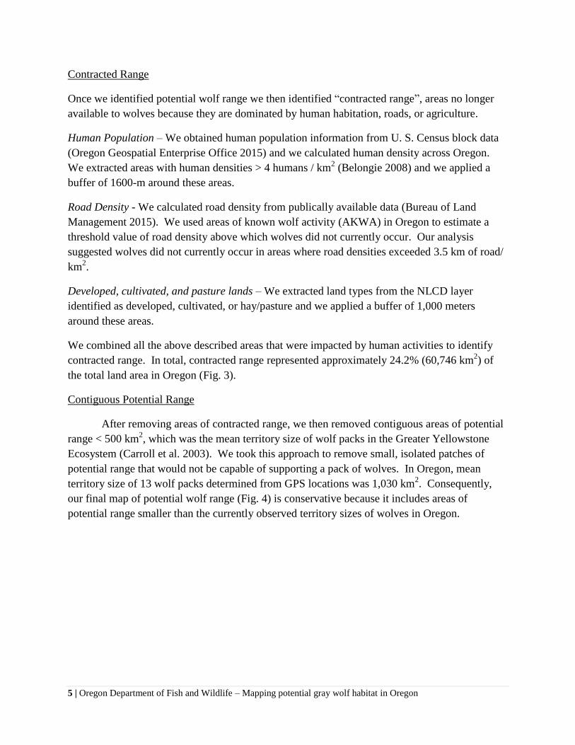
5 | Oregon Department of Fish and Wildlife – Mapping potential gray wolf habitat in Oregon
Contracted Range
Once we identified potential wolf range we then identified “contracted range”, areas no longer
available to wolves because they are dominated by human habitation, roads, or agriculture.
Human Population – We obtained human population information from U. S. Census block data
(Oregon Geospatial Enterprise Office 2015) and we calculated human density across Oregon.
We extracted areas with human densities > 4 humans / km2 (Belongie 2008) and we applied a
buffer of 1600-m around these areas.
Road Density - We calculated road density from publically available data (Bureau of Land
Management 2015). We used areas of known wolf activity (AKWA) in Oregon to estimate a
threshold value of road density above which wolves did not currently occur. Our analysis
suggested wolves did not currently occur in areas where road densities exceeded 3.5 km of road/
km2.
Developed, cultivated, and pasture lands – We extracted land types from the NLCD layer
identified as developed, cultivated, or hay/pasture and we applied a buffer of 1,000 meters
around these areas.
We combined all the above described areas that were impacted by human activities to identify
contracted range. In total, contracted range represented approximately 24.2% (60,746 km2) of
the total land area in Oregon (Fig. 3).
Contiguous Potential Range
After removing areas of contracted range, we then removed contiguous areas of potential
range < 500 km2, which was the mean territory size of wolf packs in the Greater Yellowstone
Ecosystem (Carroll et al. 2003). We took this approach to remove small, isolated patches of
potential range that would not be capable of supporting a pack of wolves. In Oregon, mean
territory size of 13 wolf packs determined from GPS locations was 1,030 km2. Consequently,
our final map of potential wolf range (Fig. 4) is conservative because it includes areas of
potential range smaller than the currently observed territory sizes of wolves in Oregon.

6 | Oregon Department of Fish and Wildlife – Mapping potential gray wolf habitat in Oregon
Figure 3. Distribution of contracted range, separated by human activities that prevent the area from being classified
as potential wolf range.

7 | Oregon Department of Fish and Wildlife – Mapping potential gray wolf habitat in Oregon
RESULTS AND SUMMARY
Our mapping process identified 106,853 km2 of potential wolf range in Oregon (Fig. 4;
Table 1). Overlaying AKWAs with our potential range map suggested our map corresponded
well with known wolf distributions (Fig. 5). The exception is an area used by the Imnaha and
Chesnimnus packs in northeast Oregon, whose AKWAs encompasses a large area of non-
forested habitat known as the Zumwalt Prairie. This area is a remnant prairie which is
productive and remote enough to support large elk herds in a non-forested environment.
However, this habitat type is not present in significant amounts elsewhere in Oregon.
Figure 4. Distribution of potential wolf range in Oregon as determined by spatial analysis conducted by Oregon
Department of Fish and Wildlife.

8 | Oregon Department of Fish and Wildlife – Mapping potential gray wolf habitat in Oregon
Figure 5. Current distribution of areas of known wolf activity compared to potential wolf range in Oregon.
Table 1. Summary of area of potential wolf range by wolf management zone in
Oregon and amount of potential range currently occupied by wolves.
Management zone Potential range (km2) Currently occupied range (km
2)
West 71,011 1,523
East 35,842 11,059
Total 106,853 12,582

9 | Oregon Department of Fish and Wildlife – Mapping potential gray wolf habitat in Oregon
Our map of potential wolf range indicates more potential range occurs in the west
management zone (71,011 km2) than the east management zone (35,842 km
2). Currently, wolves
occupy 30.9% of potential wolf range in the east management zone (11,059 km2 out of 35,842
km2 of potential range; Fig. 6). In contrast, wolves currently occupy approximately 2.1% of
potential range in the west management zone (1,523 km2 out of 71,011 km
2 of potential range).
Figure 6. Potential wolf range by wolf management zone and currently occupied potential range in Oregon.

10 | Oregon Department of Fish and Wildlife – Mapping potential gray wolf habitat in Oregon
LITERATURE CITED
Belongie, C. C. 2008. Using GIS to create a gray wolf habitat suitability model and to assess
wolf pack ranges in the western upper Peninsula of Michigan. Resource Analysis 10.
Benson, J. F., K. J. Mills, and B. R. Patterson. 2015. Resource selection by wolves at dens and
rendezvous sites in Algonquin park, Canada. Biological Conservation 182:223-232.
Bureau of Land Management. 2015. BLM OR GTRN Web Roads Line. in OR BLM, Portland,
OR, http://www.blm.gov/or/gis/data.php, accessed 3/3/2015.
Carroll, C., M. K. Phillips, N. H. Schumaker, and D. W. Smith. 2003. Impacts of landscape
change on wolf restoration success: planning a reintroduction program based on static
and dynamic spatial models. Conservation Biology 17:536-548.
Jin, S., L. Yang, P. Danielson, C. Homer, J. Fry, and G. Xian. 2013. A comprehensive change
detection method for updating the National Land Cover Database to circa 2011. Remote
Sensing of Environment 132:159-175.
Kohn, B. E., R. Thiel, and J. L. Hansen. 2001. Road density as a factor in habitat selection by
wolves and other carnivores in the Great Lakes Region. Carnivore Conservation in the
Twenty-first Century 97 18:110.
Larsen, T., and W. J. Ripple. 2006. Modeling gray wolf (Canis lupus) habitat in the Pacific
Northwest, U.S.A. Journal of Conservation Planning 2:17-33.
Mech, L. D., S. H. Fritts, G. L. Radde, and W. J. Paul. 1988. Wolf distribution and road density
in Minnesota. Wildlife Society Bulletin:85-87.
Mech, L. D., and R. O. Peterson. 2003. Wolf-prey relations. Pages 131-160 in L. D. Mech, andL.
Boitani, editors. Wolves: behavior, ecology, and conservation. The University of Chicago
Press, Chicago, IL.
Mladenoff, D. J., T. A. Sickley, R. G. Haight, and A. P. Wydeven. 1995. Landscape analysis and
prediction of wolf habitat. Conservation Biology 9:279-295.
Oakleaf, J. K., D. L. Murray, J. R. Oakleaf, E. E. Bangs, C. M. Mack, D. W. Smith, J. A.
Fontaine, M. D. Jimenez, T. J. Meier, and C. C. Niemeyer. 2006. Habitat selection by
recolonizing wolves in the northern Rocky Mountains of the United States. Journal of
Wildlife Management 70:554-563.
Oregon Geospatial Enterprise Office. 2015. Oregon Spatial Data Library,
http://spatialdata.oregonexplorer.info/geoportal/catalog/main/home.page, Accessed
2/13/2015. in.
Peterson, R. O., and P. Ciucci. 2003. The wolf as a carnivore. Pages 104-130 in L. D. Mech,
andL. Boitani, editors. Wolves: Behavior, ecology and conservation. The University of
Chicago Press, Chicago.
Zimmermann, B., L. Nelson, P. Wabakken, H. Sand, and O. Liberg. 2014. Behavioral responses
of wolves to roads: scale-dependent ambivalence. Behavioral Ecology 25:1353-1364.

Appendix B
Assessment of Population Viability of Wolves in Oregon
This technical report to the Oregon Fish and Wildlife Commission presents results from an
individual-based population model used to assess population viability of wolves in Oregon.
Suggested citation:
Oregon Department of Fish and Wildlife. 2015. Assessment of population viability of wolves in
Oregon. Oregon Department of Fish and Wildlife, 4034 Fairview Industrial Drive SE. Salem,
OR 97302.

1 | Oregon Department of Fish and Wildlife - Assessment of population viability of wolves in Oregon
TABLE OF CONTENTS
EXECUTIVE SUMMARY……………………………………………………………
INTRODUCTION……………………………………………………………………
METHODS………………………………………………………………………….
Model Parameters……………………………………………………………
Starting Population Size…………………………………………………..
Survival……………………………………………………………………
Density-dependence……………………………………………………….
Prey Multiplier……………………………………………………………
Dispersal and Emigration…………………………………………………
Territory Establishment…………………………………………………...
Immigration……………………………………………………………….
Anthropogenic Mortality………………………………………………….
Reproduction………………………………………………………………
Catastrophes………………………………………………………………
Assessment of Population Viability…………………………………………
Model Validation……………………………………………………………..
Sensitivity Analysis…………………………………………………………..
Effects of Stochastic Parameters………………………………………….
Effects of Static Parameters……………………………………………….
Effects of Lethal Control of Wolves………………………………………...
RESULTS…………………………………………………………………………..
Model Validation……………………………………………………………..
Assessment of Population Viability…………………………………………
Sensitivity Analysis…………………………………………………………..
Effects of Stochastic Parameters………………………………………….
Effects of Static Parameters………………………………………………
Effects of Lethal Control of Wolves………………………………………...
Comparison of Individual vs. Pack Removal……………………………...
DISCUSSION……………………………………………………………………….
LITERATURE CITED………………………………………………………………
4
5
5
8
8
8
11
12
12
13
13
13
13
14
14
14
15
15
15
15
16
16
16
18
18
21
26
26
29
33

2 | Oregon Department of Fish and Wildlife - Assessment of population viability of wolves in Oregon
LIST OF TABLES
Table 1. Parameter values used in an individual-based population model used to
predict future population growth of wolves in Oregon compared to values
required to match observed growth rates of Oregon’s wolf population from
2010-2014…………………………………………………………………………
Table 2. Annual survival rates and anthropogenic mortality rates of non-pup
wolves reported in literature………………………………………………………
Table 3. Survival rates of wolf pups from birth to six months reported in
literature…………………………………………………………………………..
Table 4. Results of linear regression model used to estimate sensitivity of
intrinsic growth rates of wolf populations in Oregon using an individual-based
population model………………………………………………………………….
7
9
10
19

3 | Oregon Department of Fish and Wildlife - Assessment of population viability of wolves in Oregon
LIST OF FIGURES
Figure 1. The order in which demographic processes are implemented in an
individual-based population model to assess population viability of wolves……..
Figure 2. Visual representation of the life cycle of wolves implemented in an
individual-based population model to assess population viability of wolves……..
Figure 3. Comparison of (a) simulated mean population sizes compared to
minimum population sizes observed in Oregon from 2009-2014 and (b)
simulated number of breeding pairs to minimum number of known breeding
pairs in Oregon from 2009-2014 using baseline simulation parameters or
observed model parameters……………………………………………………….
Figure 4. Estimates of cumulative probability of simulated wolf populations
reaching the conservation-failure or biological-extinction thresholds over the
next 50 years………………………………………………………………………
Figure 5. Estimated effects of significant (p < 0.05) model parameters on
intrinsic growth rates of wolf populations………………………………………...
Figure 6. Estimated effect of variation in starting population size on (a) mean
population size and (b) cumulative probability of conservation-failure over the
next 50 years………………………………………………………………………
Figure 7. Estimated effect of variation in density-threshold on (a) mean
population size and (b) cumulative probability of conservation-failure over the
next 50 years………………………………………………………………………
Figure 8. Estimated effect of variation in interval between catastrophic
reductions in survival of wolves on (a) mean population size, (b) cumulative
probability of conservation-failure, and (c) cumulative probability of biological-
extinction over the next 50 years………………………………………………….
Figure 9. Estimated effect of variation in intervals between reproductive failure
on (a) mean population size and (b) cumulative probability of conservation-
failure over the next 50 years……………………………………………………..
Figure 10. Estimated effect of variation in legal removal rates of wolves on (a)
mean population size, (b) cumulative probability of conservation-failure, and (c)
cumulative probability of biological-extinction over the next 50 years…………..
Figure 11. Estimated effect of individual versus pack level legal removal on (a)
mean population size and (b) cumulative probability of conservation-failure over
the next 50 years…………………………………………………………………..
6
6
17
18
20
22
23
24
25
27
28

4 | Oregon Department of Fish and Wildlife - Assessment of population viability of wolves in Oregon
EXECUTIVE SUMMARY
We present results from an individual-based population model (IBM) used to assess the
viability of the Oregon gray wolf (Canis lupus) population. When parameterizing our model, we
relied heavily on published estimates of wolf vital rates. We compared estimates of parameters
used in our model to those observed in Oregon from 2009-2014 and concluded our model was
conservative compared to values currently observed in Oregon. We used a starting population
size of 74 wolves which was based on preliminary wolf population counts conducted by the
Oregon Department of Fish and Wildlife (ODFW) from January 1 to 22, 2015 and this value is
slightly lower than final reported count numbers (ODFW 2015). We used linear regression
models to determine the relative effect of model parameters on intrinsic population growth rates
of wolves. We assessed population viability using two metrics: 1) the cumulative proportion of
simulations that had fewer than 4 breeding pairs (defined as conservation-failure) and 2) the
cumulative proportion of simulations that had fewer than 5 wolves (defined as biological-
extinction).
Increased pup (β = 0.045), yearling (β = 0.024), and adult (β = 0.019) survival resulted in
increased population growth rates. Population growth rates of wolves were most sensitive to
environmental stochasticity, which we modeled through the use of a prey multiplier (β = 0.088).
The increased environmental stochasticity incorporated in the model by the prey multiplier
increased variation in survival rates of wolves by up to 20% annually, which caused this
parameter to have a large effect on population growth rates. Increased levels of illegal (β = -
0.027) and legal (β = -0.028) anthropogenic mortality had negative effects on population growth
rates. Increased mean litter size had a positive effect on population growth (β = 0.049).
Increased mortality rates for dispersing wolves had a negative effect on population growth (β = -
0.026) while increased probabilities of dispersing wolves successfully establishing a territory had
a positive effect on population growth (β = 0.034). Combined, these results highlight the
importance of survival, reproduction, and human-caused mortality on population growth rates of
wolves. Other parameters considered in our model had minimal effects on population growth
rates or viability of wolves. Maintenance of high natural survival and reproductive rates of
wolves while minimizing human-caused mortality will help ensure the long-term persistence of
the species in Oregon.
Our baseline model indicated there was a 0.06 (95% CI = 0.01 – 0.11) probability of
wolves falling below the conservation-failure threshold and a 0.01 (95% CI = 0.00 – 0.03)
probability of falling below the biological-extinction threshold in the next 50 years. When we
parameterized our model with vital rates required to match population growth rates observed in
Oregon from 2009-2014, we did not observe any situations where the simulated wolf population
fell below the conservation-failure or biological-extinction thresholds. Consequently, we
contend future risk of conservation-failure falls between estimates from our baseline model (0.06
probability of conservation-failure) and our model parameterized with vital rates required to
match observed population growth rates of Oregon’s wolves from 2009-2014 (0.00 probability
of conservation-failure). Regardless of model parameterization, our results suggested it is
extremely unlikely (≤ 0.01 probability) wolves in Oregon will be at risk of complete extirpation
over the next 50 years.

5 | Oregon Department of Fish and Wildlife - Assessment of population viability of wolves in Oregon
INTRODUCTION
The Oregon Wolf Conservation and Management Plan (hereafter; Oregon Wolf Plan;
Oregon Department of Fish and Wildlife [ODFW] 2010) outlines phases of wolf (Canis lupus)
recovery and criteria for delisting wolves as required by Oregon’s Endangered Species Act
(ESA). In January 2015, Oregon’s wolf population successfully reached population objectives
for Phase I to allow ODFW to propose that the Oregon Fish and Wildlife Commission consider
delisting of wolves from Oregon’s ESA (ODFW 2010). Quantitative models are commonly used
to assess population dynamics and extinction risk of threatened and endangered species (Boyce
1992, Morris and Doak 2002) and can provide insight into the first and second delisting criteria
outlined in the Oregon ESA:
1. “The species is not now (and is not likely in the foreseeable future to be) in danger of
extinction in any significant portion of its range in Oregon or in danger of becoming
endangered”; and
2. “The species natural reproductive potential is not in danger of failure due to limited
population numbers, disease, predation, or other natural or human related factors
affecting its continued existence”.
To address these delisting criteria, we developed a quantitative model to provide insight into
dynamics of Oregon’s wolf population to help inform any future decisions regarding wolves and
Oregon’s ESA.
To make accurate predictions of future population growth, quantitative population
models should accurately reflect biological processes of the species being modeled. Individual-
based models (IBM) were previously used to model wolf population dynamics (Vucetich et al.
1997, Haight et al. 1998, Nilsen et al. 2007, Bull et al. 2009) because they can most accurately
represent the unique social and breeding structure of wolf populations. We modified an IBM
developed to assess effects of management on wolf populations in Norway (Bull et al. 2009) to
meet our needs to assess population viability of wolves in Oregon. Our modeling approach
focused on determining effects of key biological processes, uncertainty in model parameters, and
management actions on wolf population dynamics and viability.
METHODS
We used an IBM modified from Bull et al. (2009) to assess future population dynamics of
wolves in Oregon. Our model incorporated 6 demographic processes that affected wolf
populations that were modeled in the following order (Fig. 1): 1) survival and transition between
age classes, 2) dispersal and emigration out of Oregon, 3) territory establishment by dispersing
wolves, 4) immigration from outside Oregon, 5) anthropogenic mortality, and 6) reproduction.
Our IBM included 5 distinct social classifications of wolves (Fig. 2) and transitions between
social classifications were governed by distinct model parameters (Table 1).
Our model was coded and implemented in R (R Development Core Team 2012). To
generate our results, we conducted 100 realizations of population growth over 50 years. We
incorporated environmental stochasticity in our model by randomly drawing vital rate values
from a uniform distribution with a predefined mean and standard deviation at each time step of
the simulation (Table 1). Unless otherwise noted, vital rates were applied at an individual level,
which inherently incorporated demographic stochasticity into our model. For each simulated
population we tracked parameter values, population size and growth rates, and number of
breeding pairs (i.e., pairs of wolves with ≥ 2 pups surviving the biological year) at each time
step.
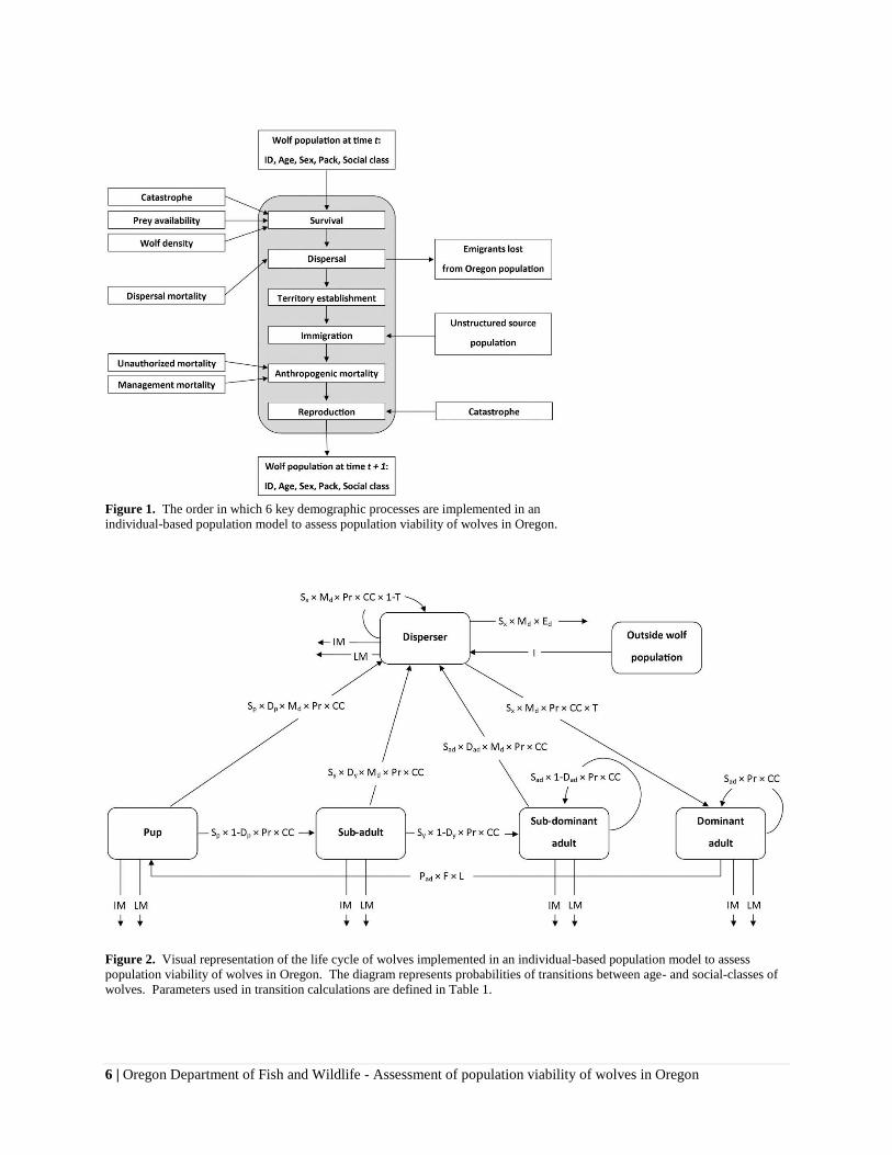
6 | Oregon Department of Fish and Wildlife - Assessment of population viability of wolves in Oregon
Figure 1. The order in which 6 key demographic processes are implemented in an
individual-based population model to assess population viability of wolves in Oregon.
Figure 2. Visual representation of the life cycle of wolves implemented in an individual-based population model to assess
population viability of wolves in Oregon. The diagram represents probabilities of transitions between age- and social-classes of
wolves. Parameters used in transition calculations are defined in Table 1.

7 | Oregon Department of Fish and Wildlife - Assessment of population viability of wolves in Oregon
Table 1. Parameter values used to predict future population growth of wolves in Oregon compared to values required to match observed growth
rates of Oregon's wolf population from 2010-2014. Values used at each time step of the analysis were randomly drawn from a uniform
distribution within the specified standard deviation (SD). Mean values are probabilities unless otherwise stated.
Baseline model
values
Values required to match
growth rates observed in
Oregon (2009-2014)
Parameter Notation Mean SD Mean SD
Pup survival rate Sp 0.68 0.15
0.75 0.05
Yearling survival rate Sy 0.81 0.06
0.91 0.04
Adult (2 to 7-yrs old) survival rate Sad 0.88 0.04
0.91 0.04
Old adult (8 to 9-yrs old) survival rate Sold 0.63 0.11
0.85 0.05
Pup dispersal rate Dp 0.15 0.05
0.15 0.05
Yearling dispersal rate Dy 0.65 0.05
0.65 0.05
Non-breeding adult dispersal rate Dad 0.65 0.05
0.65 0.05
Proportion of dispersing wolves that survive Md 0.90 0.05
0.97 0.02
Proportion of dispersing wolves that leave Oregon Ed 0.115 0.03
0.115 0.03
Probability of dispersing wolf establishing a territory T 0.75 0.10
0.75 0.10
No. of immigrants arriving annually from outside Oregon I 3 2
3 2
Pregnancy rate for dominant females Pad 0.95 0.02
0.95 0.02
Litter size L 5 3
5 3
Proportion of wolves removed by illegal mortality IM 0.05 0.03
0.02 0.01
Proportion of wolves removed by legal mortality LM 0.05 0.03
NA NA
Prey index multiplier (adjustment to survival rates) Pr 1.00 0.10
1.00 0.10
Density dependent threshold (no. of wolves) CC 1,500 NA
1,500 NA
Probability of population wide reduction in survival Scas 0.01 NA
NA NA
Probability of pack-specific reproductive failure Rcas 0.05 NA 0.05 NA
8 | Oregon Department of Fish and Wildlife - Assessment of population viability of wolves in Oregon
Model Parameters
Currently, Oregon has minimal vital rate information to parameterize a population model,
and the potential for sampling bias or error from small sample sizes (i.e., observed data does not
match the expected outcome) could cause inappropriate conclusions to be reached by using this
information. Furthermore, estimated vital rates from protected wolf populations that are
colonizing or recovering are unlikely to match those of established wolf populations (Ballard et
al. 1987, Hayes and Harestad 2000, Fuller et al. 2003). Oregon’s wolf population is beginning to
transition from a recovering to established population. Consequently, vital rates used in our IBM
were obtained primarily from studies conducted in established wolf populations. However,
whenever possible, we compared vital rates obtained in Oregon to those reported in literature to
determine the degrees to which vital rates used in our model were representative of those
observed in Oregon since 2009. In general, most vital rates used in our baseline model were
conservative compared to those observed in Oregon from 2009-2014. Using conservative vital
rate estimates allowed us to err on the side of caution (e.g., the precautionary principle; Myers
1993, Meffe et al. 2006) and prevent overly optimistic conclusions of wolf population viability.
Starting Population Size.–We utilized preliminary wolf population count data collected from
January 1-22, 2015 by ODFW to determine our starting population size and structure and these
preliminary counts were lower than final survey numbers (ODFW 2015). At the time
preliminary counts were conducted, a minimum of 74 wolves were present in Oregon. We
acknowledge additional, undocumented wolves may be present in Oregon, but we relied on
known individuals when developing our model. Preliminary counts indicated there were a total
of 13 pairs or packs of wolves in addition to 2 individual wolves present in Oregon. Whenever
possible, we used existing data to assign pack, age, social class, and sex of wolves and randomly
assigned these attributes when unknown. Newly documented pairs of wolves were assumed to
consist of a male and female and both individuals were assigned dominant-adult status.
Survival.–Baseline survival rates of wolves used in our model represented survival in the
absence of anthropogenic mortality (e.g., poaching, management removals). We adjusted
survival rates reported in literature to account for anthropogenic mortality using the following
approach: 1) determine the overall mortality rate (1 – survival rate), 2) estimate the
anthropogenic mortality rate as the product of proportion of total mortalities caused by humans
and the overall mortality rate, and 3) sum the estimated anthropogenic mortality rate and the
reported survival rate. As an example, Smith et al. (2010) reported an annual survival rate of
0.750 with 54% of mortality attributable to legal or illegal actions by humans. The
anthropogenic mortality rate was 0.135 (1-0.750 × 0.540), which resulted in a ‘natural’ survival
rate of 0.885 (0.750 + 0.135). In instances where authors directly reported cause-specific
mortality rates (e.g., Wydeven et al. 1995), we summed reported survival and anthropogenic
mortality rates to obtain an adjusted estimate of survival. After adjusting survival rates reported
in literature (Table 2) we arrived at a survival rate of 0.88 (± 0.04 SD) of adult wolves (2-7 years
old; Sad) for use in our model.
Using the largest sample size of radio-collared wolves reported in published literature,
Smith et al. (2010) reported that yearling wolves had a 54.9% higher risk (1.0012365
= 1.549) of
mortality than adult wolves over 365 days. We adjusted the mean survival rate of 0.88 for adult
(2-7 years) wolves by the increased hazard rate reported by Smith et al. (2010) to calculate a
survival rate of 0.81 for yearling wolves (Sy; 1-[(1-0.88) × 1.549]; Table 1). This may present
an overly pessimistic view of resident yearling wolf survival, because yearlings have high
dispersal rates (Gese and Mech 1991) and dispersing wolves were found to have higher risk of

9 | Oregon Department of Fish and Wildlife - Assessment of population viability of wolves in Oregon
mortality (Smith et al. 2010). In our model, we utilized a separate mechanism to account for
increased mortality of dispersing wolves (see below) and we recognize our estimates of yearling
survival may be negatively biased. Senescence, observed through decreased survival at older
ages is common for large mammals (Loison et al. 1999, Gaillard et al. 2000, Clark et al. 2014),
but this phenomenon is not well documented in wolves. Cubaynes et al. (2014) reported an
annual survival rate for wolves > 7 years old of 0.63, which we adjusted to 0.67 for use in our
model (Sold) to account for anthropogenic mortality. Wolves ≥ 10 years of age had a survival
rate of 0.00 in our model. While free-ranging wolves can live longer than 10 years, most wolves
are typically no longer reproductively active after this age (Fuller et al. 2003, Kreeger 2003) and
will contribute little to population growth and viability.
Estimates of non-pup survival used in our model were lower than observed to date in
Oregon. Using known-fate survival analysis (White and Burnham 1999) on a sample 23 of
wolves radio-collared in Oregon from 2009-2014, we estimated an annual survival rate of wolves
> 6 months old of 0.91. Three collared wolves died during this timeframe, one of which was
removed by ODFW and an additional wolf was illegally shot resulting in 66% of mortality being
attributable to humans. Adjusting survival rates to account for anthropogenic mortality results in
a survival rate of 0.97, which is substantially greater than the adult (0.88) and yearling (0.81)
survival rates used in our model.
Table 2. Annual survival rates and human-caused mortality rates of non-pup wolves reported in
literature. Survival rates were estimated from known fates of radio-collared wolves unless otherwise
noted. Adjusted survival rates represent survival rates on non-pups in the absence of human-caused
mortality.
Source
Reported
survival
Human-caused
mortality rate Adjusted survival ratea
Adams et al. (2008) 0.79 0.09b 0.89
Cubaynes et al. (2014) 0.80 0.04c 0.84
Fuller (1989) 0.62 0.26c 0.88
Hayes and Harestead (2000) 0.84 0.02b 0.86
Peterson et al. (1984) 0.67 0.26b 0.93
Smith et al. (2010) 0.75 0.14b 0.89
Webb et al. (2011)d 0.62 0.34
b 0.96
Wydeven et al. (1995) 0.61 0.28b 0.89
Wydeven et al. (1995) 0.82 0.04b 0.86
Mean 0.72 0.16 0.88 a Sum of reported survival and human-caused mortality rate.
b Mortality rate calculated as the product of overall mortality rate (1-survival) and proportion of
mortalities caused by humans. c Human-caused mortality rate directly reported by authors.
d Apparent survival rates estimated from mark-recapture data.

10 | Oregon Department of Fish and Wildlife - Assessment of population viability of wolves in Oregon
Estimates of survival of wolf pups from birth to 6 months are highly variable and are
usually estimated by comparing pup counts at den or rendezvous sites to in utero fetal counts of
harvested females. Based on a review of literature (Table 3), we determined mean survival rates
of wolf pups from birth to 6 months, determined from pup counts, were 0.73. Estimation of
survival using pup count data assumes that pups are counted with a detection probability of 1.0,
which is unrealistic and this method will likely produce negatively biased estimates of survival
over the first 6 months of life. In general, radio-telemetry studies have indicated pup survival is
similar to adult survival during months 7-12 after birth (Peterson et al. 1984, Fuller 1989, Adams
et al. 2008). Consequently, we used 6 month survival rate of adults (~0.94), calculated as the
square root of annual survival, to approximate survival of pups from ages 7-12 months. We used
the product of summer survival rates times the 6 month survival rate of adult wolves as the
annual estimate of pup survival (Sp) in our baseline model (0.73 × 0.94 = 0.68; Table 1).
Table 3. Survival rates of wolf pups from birth to six months reported in literature. Unless otherwise
noted, survival was estimated by comparing pup counts six months after birth to in utero litter sizes.
Annual survival rates calculated as the product of 6 month survival rates of pups and 6 month survival
rates of adult wolves used in our model (0.88).
Source
Survival from birth to 6
months Annual survivala
Fuller (1989)b 0.58 0.55
Mills et al. (2008)c 0.83 0.78
Fritts and Mech 0.57 0.53
Fuller and Keith (1980) 0.69 0.65
Adams et al. (2008) 0.81 0.76
Hayes and Harestead (2000)d 0.80 0.75
Petersen et al. (1984) 0.80 0.75
Ballard et al. (1987) 0.82 0.77
Mech et al. (1998)e 0.91 0.85
Hayes et al. (1991)f 0.48 0.45
Mean survival 0.73 0.68 a Annual survival is the product of survival from birth to 6 months and the 6 month survival rate of
adult wolves used in our model. b Survival rate reported was estimated over 8 month period using pup counts. Monthly survival rate
was 0.9135 and survival over six months was 0.58. c Survival was estimated with implant transmitters from Jun-Nov. Used monthly survival rates from
this period to estimate 6 month survival rate. d Survival estimated on an annual interval. Used the square root of reported survival rates to estimate
survival from birth to 6 months. e Survival estimate over first 4 months of life. Extrapolated to 6 months.
f Heavily exploited wolf population.

11 | Oregon Department of Fish and Wildlife - Assessment of population viability of wolves in Oregon
We compared the pup survival rates used in our model to pup count data collected in
Oregon during winter surveys conducted from 2009-2014. During this time frame, 30 potential
reproductive opportunities were documented. Of these 30 potential reproductive opportunities, 3
were censored because final pup counts were not completed. Assuming wolves give birth to an
average of 5 pups per litter (Fuller et al. 2003), we calculated a total of 135 pups born from these
27 reproductive opportunities. Minimum pup counts conducted in December of 2009-2014
indicated a minimum of 82 pups across all years. Using this information we arrived at a
minimum observed survival rate of 0.61 (95% CI = 0.53 – 0.69), which is lower but within in the
range of the pup survival rate used in our model (0.68 ± 0.15; Table 1).
When implementing our model, annual survival rates were independently calculated for
each age class by randomly drawing a survival rate from a uniform distribution with a predefined
mean and standard deviation (Table 1). Survival rates of wolves were age-specific and were not
influenced by social status of the individual (e.g., survival rates for a 4-year old sub-dominant
adult were identical to survival rates for a 4-year old dominant adult). Survival rates were
modeled at an individual level, with each individual having an independent probability of
survival at each time step.
Density-dependence.– When populations surpassed a predefined population threshold, annual
survival rates, regardless of age, were multiplied by the ratio of the threshold population size and
current wolf population size. The specified threshold was implemented to account for the
importance of density-dependence on population dynamics (Morris and Doak 2002), but does
not represent an expected number of wolves in Oregon in future years. When implemented in
our model, the density-threshold represents an arbitrary biological threshold where wolves begin
to self-regulate through intraspecific strife or are limited by available prey.
Larsen and Ripple (2006) created a habitat suitability map for wolves in Oregon and
found that a maximum of 1,450 wolves could occupy Oregon. This value increased to 2,200
wolves if industrial timberland in western Oregon was classified as suitable wolf habitat. Fuller
et al. (2003) provided the following equation to estimate expected wolf densities:
Wolves/1,000 km2 = 3.5 + 3.27 × U
, where U is the ungulate biomass index (km2). Using an estimated elk (Cervus elaphus)
population of 128,000 elk distributed across 151,500 km2
of summer range habitat (ODFW,
unpublished data) and assigning each elk a biomass value of 3, results in a value of U of 2.53
(128,000 × 3/151,500). Based on this value maximum wolf densities were estimated to be 11.79
wolves/1,000 km2 of summer range elk habitat. This would result in a total population of 1,780
wolves within 151,500 km2 of elk summer range habitat in Oregon. Carbone and Gittleman
(2002) provided the following equation to estimate wolf densities based on available primary
prey biomass:
Number of wolves = 0.62 × primary prey biomass
, where primary prey biomass is scaled per 10,000 kg. Currently, Oregon’s elk population is
approximately 128,000 with each elk weighing on average 217 kg (ODFW, unpublished data).
This results in approximately 2,777.6 × 10,000 kg of primary prey biomass available to wolves
across Oregon and a maximum population estimate of approximately 1,722 wolves.
Both the Fuller et al. (2003) and Carbone and Gittleman (2002) equations produce similar
estimates of wolf population size and fall within the range reported by Larsen and Ripple (2006).
However, these estimates were calculated under the assumption wolves will not cause reductions
in prey populations. To account for this possibility, we used a conservative density-threshold
(CC) of 1,500 wolves in our model. Again, it should be noted, the density-threshold represents

12 | Oregon Department of Fish and Wildlife - Assessment of population viability of wolves in Oregon
an estimate of maximum potential wolf population size, not a management objective for wolves
in Oregon.
Prey multiplier.–Wolf-prey interactions can influence wolf densities and population
dynamics (Fuller et al. 2003). We lacked sufficient data to explicitly model wolf-prey
interactions and instead used a simplified approach described by Bull et al. (2009) where a
stochastically generated a prey multiplier value (Pr) was used to represent changes in either prey
abundance or vulnerability (e.g., increased vulnerability during severe winters). The prey
multiplier represented environmental stochasticity in our model. At a value of 1.0, the prey
multiplier represented baseline prey availability or vulnerability. Each year of the simulation,
the prey multiplier had a 1 out of 3 chance of increasing, decreasing, or remaining the same,
respectively. In years the prey multiplier increased or decreased, the maximum change was
restricted to 0.10. The prey multiplier was bounded between 0.90 and 1.10 values generated
outside this range were truncated to the maximum or minimum value. Survival rates used in the
model were calculated as the product of randomly drawn survival rates and the prey multiplier
after accounting for any density-dependent effects.
Dispersal and Emigration.–We assumed dominant wolves would maintain their territory and
breeding positions until their death. In the event that both dominant animals in a pack died, all
remaining pack members would disperse. This approach was partially used for simplicity of
model implementation, but is also supported in literature (Fuller et al. 2003). For example,
Brainerd et al. (2008) found that in instances where both breeding wolves were lost, 85% of
packs dissolved, and only 9% of packs reproduced the following year.
Sub-dominant wolves that survived the year had a probability of dispersing from their
existing territory, which was dependent on age and breeding status (Table 1). Age-specific
dispersal rates used in our model (Dp, Dy, Dad) were obtained from literature (Potvin 1988, Fuller
1989, Gese and Mech 1991). We assumed non-breeding adults had similar dispersal rates as
yearlings (Fuller et al. 2003). Survival rates of dispersing individuals were reduced (Md) to
account for increased mortality risk of wolves during dispersal (Table 1; Peterson et al. 1984,
Fuller 1989, Smith et al. 2010). Smith et al. (2010) found dispersing wolves had a 38.9% higher
risk of mortality over 365 days than resident wolves. After accounting for this increased risk,
survival rates of dispersing adult wolves would be 0.83 with the ratio of dispersing versus
resident adult survival rates of 0.94 (0.83/0.88). To be conservative, we lowered this value to
0.90 (± 0.05 SD) for use in our model, which is interpreted at 10% of dispersing wolves die
during the dispersal process.
We used a spatial simulation to estimate emigration rates using published estimates of
dispersal distances of wolves (Fritts and Mech 1981, Fuller 1989, Gese and Mech 1991,
Wydeven et al. 1995). We generated 10,000 random dispersal paths that started at a random
location within summer range elk habitat (i.e., potential wolf habitat). We simulated dispersal
paths using correlated random walks with the movement.simplecrw function in the Geospatial
Modeling Environment (Beyer 2012) by selecting a random bearing from a uniform distribution
(0 - 359°) and a random dispersal distance from normal distribution with a mean of 75 km (± 30
SD). We calculated emigration rates (Ed) as the proportion of simulated dispersal paths that
terminated outside Oregon. Mean emigration rates were estimated to be 0.115 (Table 1). We
estimated a standard deviation of the mean values calculated from 100 bootstrap samples that
each contained 100 random dispersal paths. The estimated standard deviation of the mean of
these 100 samples was 0.03. Emigration was effectively treated as additional mortality in our
model (i.e., these individuals were removed from the simulated population).

13 | Oregon Department of Fish and Wildlife - Assessment of population viability of wolves in Oregon
Territory Establishment.–Dispersing wolves ≥ 2 years old were assigned a probability of
establishing a territory. Boyd and Pletscher (1999) found that 57% of dispersing wolves
successfully found a mate the next breeding season after they dispersed. This value equates to
the joint probability of two wolves establishing a territory. Independently, the probability of a
dispersing wolf establishing a territory (T) would be 0.75 (√0.57), which we used in our model.
Wolves that did not successfully establish a territory remained in the pool of dispersers until the
following year. Those individuals that successfully established territories would first fill vacant
alpha positions of the correct sex in established packs. If no alpha positions were available at
established packs, dispersing wolves would then establish a new territory and maintain that
position until they died or a mate joined them at the territory.
Immigration.–We assumed wolves from the extant Rocky Mountain wolf population would
be available to immigrate into Oregon. For model simplification, we assumed the wolf
population outside Oregon was unstructured and would produce a steady, but limited, stream of
immigrants. We assumed 3 wolves (± 2 SD) would arrive immigrate (I) annually into Oregon
from surrounding populations. We assumed all immigrating wolves were sub-adults because this
age class is most likely to engage in dispersal behavior (Fuller 1989, Gese and Mech 1991, Fuller
et al. 2003). Individuals arriving in the Oregon population were randomly assigned a sex
assuming parity among dispersers (Gese and Mech 1991).
Anthropogenic Mortality.–Anthropogenic mortality was incorporated in the model under two
forms: legal and unauthorized mortality. Unauthorized mortality represented all sources of
anthropogenic mortality (e.g., poaching, vehicle-killed individuals) excluding mortalities
authorized by ODFW under current laws. Legal removals included any administrative removals
authorized by ODFW (e.g., livestock damage, human safety, incidental take). Anthropogenic
mortality was modeled using a two-step process where unauthorized mortality was modeled first
and followed by legal mortality. A proportion of the total population that remained after
accounting for natural mortality events would be removed each year by each anthropogenic
mortality source (Table 1). Anthropogenic mortality was applied independent of age, social
status, or pack membership. Effectively, this approach treats anthropogenic mortality as a
reduction in survival. For example, using an annual adult survival rate of 0.88, survival rates
would be reduced to 0.79 (0.88 × 0.95 × 0.95) if 5% of the population was removed for both
legal and unauthorized mortality, respectively.
From April 2009 to March 2014, ODFW has collected 45 wolf-years of data from radio-
collared individuals. During this time, 1 radio-collared wolf was illegally killed and 1 radio-
collared wolf was removed by ODFW, for a removal rate of 0.02 for each mortality source
(ODFW, unpublished data). Due to the potential bias of radio-collared wolves being avoided by
poachers, we increased the illegal mortality (IM) value to 0.05 (± 0.03 SD). To be conservative
and allow for the potential of increased levels of lethal control actions, we used a value of 0.05
(± 0.03 SD) for legal mortality (LM) of wolves in our model (i.e., between 2-8% of wolves
would be randomly removed from the population each year for management related actions).
Reproduction.–Only established wolf packs with a dominant pair of adults were allowed to
reproduce. We were unable to find reported estimates of pregnancy rates of dominant females in
published literature; however, it is biologically unrealistic to assume all pairs of wolves
successfully give birth to pups each year (i.e., female do not always become pregnant). We
assumed pregnancy rates of dominant females (Pad) would be 0.95 (± 0.02 SD; Table 1). While
evidence exists of multiple females producing pups within a pack, this is a rare occurrence and
usually only occurs in extremely large packs (Mech 1999), and we assumed only one litter of

14 | Oregon Department of Fish and Wildlife - Assessment of population viability of wolves in Oregon
pups would be born in packs with a dominant pair. The number of pups produced by pregnant
females (L) was drawn from a uniform distribution ranging from 2-8 (Table 1) based on a review
of literature (see summary in Fuller et al. 2003).
Catastrophes.–We included two catastrophes in our model. The first was modeled at the
pack level as the probability of a pack having complete reproductive failure within a year (Rcas).
Probability of reproductive failure was independent among packs and years. This approach was
used to simulate the potential effects of diseases (e.g., canine parvovirus), which are known to
negatively affect pup survival and recruitment (Mech and Goyal 1993, Almberg et al. 2009),
where most or all pups die when exposed to the virus (Mech et al. 2008). We assumed complete
reproductive failure had a probability of occurrence of 0.05 within each pack during each year of
the simulation (i.e., one out of 20 litters will be subjected to complete reproductive failure).
Packs that had complete reproductive failure were assigned a litter size of 0 (i.e., even if pups
were produced they would all die before 1 year of age).
Our second catastrophe was modeled at the population level, where each year of the
simulation there was a probability of a population wide reduction in survival (Scas). This
approach was used to represent extremely rare, range wide events that may affect wolf
populations (e.g., disease, abiotic conditions, prey population crashes). We used a mean interval
of 100 years between disturbance events, with each year having an independent probability of a
disturbance event occurring. During years where a catastrophe event occurred, survival rates of
all wolves in the population were reduced by 25%.
Assessment of Population Viability
We assessed population viability using two measures. The Oregon Wolf Plan defined a
threshold of 4 breeding pairs for 3 consecutive years as a guideline to consider delisting wolves
from the Oregon ESA (ODFW 2010). If future populations dropped below 4 breeding pairs
wolves could be considered for relisting under the Oregon ESA. Consequently, we defined
“conservation-failure” as a simulated population that fell below 4 breeding pairs. For each
simulated population, we determined which time-step, if any, that the population reached the
conservation-failure threshold. Populations that dropped below the conservation-failure
threshold were considered failures in all remaining time steps. We calculated risk of
conservation-failure as the cumulative proportion of simulated populations that had < 4 breeding
pairs.
We used a threshold of < 5 wolves as our metric of “biological-extinction”. In
simulations with < 5 wolves, the extant population would effectively be extirpated and
immigrants from outside sources would be maintaining the Oregon population. For each
simulated population, we determined the time-step, if any, that the population dropped below the
biological-extinction threshold. Once the population dropped below this threshold it was
determined to be biologically-extinct for all remaining time steps. We calculated biological-
extinction rates as the cumulative proportion of simulated populations that < 5 wolves.
Model Validation
To validate our baseline model, we conducted a set of 100 simulations over 5 years,
where the starting population size was the number of wolves present in Oregon at the end of
2009 (N = 14 wolves). We calculated the mean number of wolves and breeding pairs from
simulations and compared these values to population counts conducted by ODFW from 2010-
2014. Survival rates used in our baseline model were more conservative than observed in
Oregon from 2010-2014. Consequently, we conducted a second set of simulations where we
parameterized our model with vital rates required to match observed population growth rates in

15 | Oregon Department of Fish and Wildlife - Assessment of population viability of wolves in Oregon
Oregon from 2009-2014 (see Table 1 for differences between vital rates in the two scenarios).
Using observed vital rate values in our model would allow us to determine if our overall model
structure allowed accurate estimation of population growth under known conditions.
Sensitivity Analysis
Effects of Stochastic Parameters.– We used r (i.e., intrinsic rate of increase) as the dependent
variable in a linear regression model where stochastically varying parameters and relevant
interactions were used as independent variables. We conducted 200 realizations of population
growth over a 5-yr period which resulted in 1,000 random combinations of parameter values and
associated intrinsic growth rates (r). The sensitivity analysis was limited to a 5-yr span because
allowing population simulations to last longer than 5-yrs could cause some simulations to reach
the density-threshold of 1,500 wolves and confound the effect of parameter variation and
density-dependence on r. For each simulation, the starting population was assumed to be 120
wolves equally distributed among 20 packs. We used this starting population size because at
extremely small population sizes (e.g., N < 10) immigration of wolves could produce
biologically unreasonable population growth rates (e.g., λ > 2.0) and confound our ability to
detect an effect of parameters on r. Prior to running our regression model, all independent
variables were standardized (standardized value = [observed value - mean value]/standard
deviation) to allow direct comparisons between results. We used an alpha level of 0.05 to
determine significance of parameters and the sign and slope of beta coefficients to determine the
strength and relative effect of the parameter on r.
Effects of Static Parameters.–Starting population size, density-threshold, and frequency of
survival and reproductive catastrophes were static parameters in our model and the effects of
these were not included in our regression analysis used to determine the relative effects of
parameters on r. Consequently, we conducted additional simulations where values of static
parameters differed among simulations. Each simulation used 100 realizations of population
growth over 50 years and was parameterized with baseline values except for changes in the static
parameter of interest. We conducted 4 simulations to determine the effect of starting population
sizes of 50 wolves, the known existing Oregon wolf population (N = 74; baseline value), 100
wolves and, 150 wolves. Simulations with starting populations of 50, 100, and 150 wolves were
structured as follows: 1) each wolf belonged to a pack and each pack had 5 members with 2 of
those members being dominant adults and 2) sex, age, and social class of remaining wolves were
randomly assigned. To determine the relative influence of the density-threshold on population
viability of wolves, we conducted a set of simulations where used a density-threshold of 250,
500, 1000, 1500 (baseline value), and 2000 wolves. We conducted an additional set of 4
simulations where we investigated probabilities of individual pack reproductive failure of 0.00
(i.e., never occurs), 0.05 (baseline value), 0.10 (once every 10 years), and 0.20 (once every 5
years). We investigated the effects catastrophic reductions in survival at year-specific
probabilities of 0.00 (i.e., never occurs), 0.01 (baseline value), 0.02 (once every 50 years), 0.05
(once every 20 years), and 0.10 (once every 10 years).
Effects of lethal control of wolves Legal, anthropogenic mortality is the parameter included in our model over which
ODFW has the most control. To address the effects of varying rates of legal wolf removal on
wolf population viability we conducted a set of 6 simulations where mean legal mortality rates
and associated standard deviations varied among simulations while all other model parameters
were left at baseline values (Table 1). The following values were used as mean values (± SD) to
represent legal anthropogenic mortality rates in the 6 simulations: 0.00 (± 0.00), 0.025 (± 0.015),

16 | Oregon Department of Fish and Wildlife - Assessment of population viability of wolves in Oregon
0.05 (± 0.03), 0.10 (± 0.06), 0.15 (± 0.09), and 0.20 (± 0.12). These levels of legal mortality
rates were in addition to illegal mortality rates which were set at a mean value of 0.05 (± 0.03)
during all simulations.
Our baseline model assumes legal removals will be implemented through random
removal of individual wolves. However, the potential exists that lethal control actions could take
place across entire wolf packs, rather than individuals. Consequently, we also conducted a
simulation where legal removal of wolves would occur at a pack rather than individual level.
We assumed the proportion of packs removed per year would be the same as the proportion of
individuals removed in our baseline simulation (0.05 ± 0.03). After completion of simulations,
we compared the results to the baseline simulation to determine what effect, if any, pack removal
would have on population dynamics compared to individual removal.
RESULTS
Model Validation
Our baseline model resulted in underestimates of population size (Fig. 3a) and number of
breeding pairs (Fig. 3b) compared to population count data collected in Oregon from 2010-2104.
When our model was parameterized with survival rates of wolves observed from 2009-2014
(Table 1) the simulation results closely approximated observed population size and number of
breeding pairs. Consequently, survival rates used in our baseline model are cautious compared
to past survival rates in Oregon; however, the ability of the model to correctly predict past
population dynamics when parameterized with observed survival rates suggests other parameters
included in the model accurately portray wolf population dynamics in Oregon. Our baseline
model predicted a lower population growth rates compared to the model parameterized with
survival rates observed from 2009-2014. This suggests our baseline model will underestimate
wolf population growth and viability if survival rates from 2009-2014 are observed into the
future.
Assessment of Population Viability
Using our baseline model, simulated wolf populations increased an average of 7% (i.e., λ
= 1.07 ± 0.17 SD) per year. Over the next 50 years, there was a 0.06 (95% CI = 0.01 – 0.11)
probability of the population reaching the conservation-failure threshold (Fig. 4). Most
conservation-failures occurred within the first 10 years and by year 25 no additional populations
passed the threshold. Of the six simulated populations that fell below the conservation-failure
threshold, all eventually surpassed 4 breeding pairs in the future with these populations having
13, 26, 27, 51, 219, and 231 breeding pairs by year 50, respectively. Our baseline model
indicated there was an extremely low probability (0.01; 95% CI = 0.00 – 0.03) of wolf
populations becoming biologically-extinct in the next 50 years. One simulated population
dropped to 4 wolves in year 25; however, by year 50, this simulated population had recovered to
276 individuals.

17 | Oregon Department of Fish and Wildlife - Assessment of population viability of wolves in Oregon
Figure 3. Comparison of (a) simulated mean population sizes compared to minimum population sizes observed in
Oregon from 2009-2014 and (b) simulated number of breeding pairs to minimum number of known breeding pairs
in Oregon from 2009-2014 using baseline simulation parameters (dashed line) or observed model parameters (solid
line). Black dots represent observed wolf population size and number of breeding pairs determined from annual
surveys of wolf populations conducted by ODFW. Polygons around simulated mean population sizes and number
of breeding pairs represent 95% confidence intervals.

18 | Oregon Department of Fish and Wildlife - Assessment of population viability of wolves in Oregon
Figure 4. Estimates of cumulative probability of simulated wolf populations reaching the conservation-failure (< 4 breeding
pairs) or biological-extinction (< 5 wolves) thresholds over the next 50 years in Oregon. Estimates were generated using our
baseline model parameterization with 100 realizations of population growth over 50 years. Cumulative probabilities represent
the cumulative proportion of simulations that crossed the threshold of interest.
Using observed survival rates of wolves from 2009-2014 in our population model
resulted in no scenarios where wolf populations reached the conservation-failure or biological-
extinction thresholds. Our baseline model is more likely to represent future population dynamics
of wolves, but may be overly pessimistic, especially in the near future, given recently observed
survival rates of wolves in Oregon. Consequently, we contend future risk of conservation-failure
likely falls somewhere between our baseline model (0.06) and our model parameterized with
vital rates required to match observed population growth rates from 2009-2014 (0.00). Our
model results suggest it is extremely unlikely (≤ 0.01 probability) wolves in Oregon will be at
risk of complete extirpation over the next 50 years.
Sensitivity Analysis
Effects of Stochastic Parameters.–Nine out of 17 stochastic parameters included in our
baseline model had a significant effect on intrinsic growth rates as measured by r, and no
significant interactions between parameters were documented (Table 4). Most significant effects
(Fig. 5) were directly or indirectly related to survival rates. Survival rates of pups (Sp; β =
0.045), yearlings (Sy; β = 0.024), and adults (Sad; β = 0.019) were positively associated with r.
The prey multiplier (Pr) increased variation in survival rates of all age classes of wolves by up to
20% and resulted in the prey multiplier, which represented increased environmental
stochasticity, having the greatest effect on r (β = 0.088). Illegal (IM; β = -0.027) and legal (LM;
β = -0.028) anthropogenic mortality were negatively associate with r.

19 | Oregon Department of Fish and Wildlife - Assessment of population viability of wolves in Oregon
Table 4. Results of linear regression model used to estimate sensitivity of intrinsic growth rates of wolf populations
in Oregon using an individual-based population model. Standardized regression coefficients with associated
standard errors estimated from the full model are provided. Significance is determined as follows: *** = P < 0.001,
** = P < 0.01, * = P < 0.05, and NS = P > 0.05.
Parameter Standardized βi SE P-value Significance
Pup survival 0.045 0.007 0.000 ***
Yearling survival 0.024 0.007 0.000 ***
Adult (2 to 7-yrs old) survival 0.019 0.007 0.006 **
8-yr old adult survival -0.006 0.007 0.411 NS
9-yr old adult survival -0.002 0.007 0.789 NS
Pup dispersal 0.007 0.007 0.295 NS
Yearling dispersal 0.010 0.007 0.155 NS
Adult dispersal -0.001 0.007 0.833 NS
Proportion of dispersing wolves that die -0.026 0.007 0.000 ***
No. of immigrants arriving annually 0.009 0.005 0.109 NS
Proportion of dispersing wolves that emigrate -0.005 0.007 0.443 NS
Proportion of dispersing wolves that successfully
establish a territory 0.034 0.006 0.000 ***
Pregnancy rate for dominant females 0.001 0.007 0.912 NS
Mean litter size 0.049 0.004 0.000 ***
Prey index multiplier 0.088 0.005 0.000 ***
Illegal mortality -0.027 0.007 0.000 ***
Legal mortality -0.028 0.007 0.000 ***
Pup survival × Prey multiplier index -0.011 0.009 0.198 NS
Yearling survival × Prey multiplier index 0.000 0.009 0.958 NS
Adult survival × Prey multiplier index -0.003 0.009 0.737 NS
Pup survival × Illegal mortality -0.004 0.012 0.720 NS
Yearling survival × Illegal mortality 0.012 0.012 0.293 NS
Adult survival × Illegal mortality 0.016 0.011 0.146 NS
Pup survival × Legal mortality -0.003 0.012 0.797 NS
Yearling survival × Legal mortality 0.001 0.012 0.912 NS
Adult survival × Legal mortality 0.011 0.012 0.342 NS
Pup survival × Dispersal mortality -0.013 0.011 0.248 NS
Yearling survival × Dispersal mortality 0.003 0.012 0.824 NS
Adult survival × Dispersal mortality 0.003 0.011 0.785 NS

20 | Oregon Department of Fish and Wildlife - Assessment of population viability of wolves in Oregon
Figure 5. Estimated effects of significant (p < 0.05) model parameters on intrinsic growth rates of wolf populations. Estimates were generated using
baseline model parameterization. Results generated from 1,000 unique combinations of model parameters and associated intrinsic growth rates. Model
parameters are standardized to allow direct comparison among parameters. Black line represents estimated regression line. Gray dots represent
individual parameter estimates and associated population growth rate.

21 | Oregon Department of Fish and Wildlife - Assessment of population viability of wolves in Oregon
Increased mortality rates of dispersing wolves (Md; β = -0.026) had a negative effect on r.
This parameter negatively affected r in two ways: 1) wolves were directly removed from the
population and 2) fewer wolves were available to establish territories and contribute to
population level reproduction. Increased probabilities of dispersing wolves successfully
establishing a territory had a positive effect on r (T; β = 0.034). Mean litter size (L; β = 0.049)
was positively correlated with r. Pregnancy rates of dominant females (Pad) were not
significantly associated with r. We likely did not find a significant effect of pregnancy rates
because of the high mean value (0.95) and low variation (SD = 0.02) used in our model.
Dispersal rates, regardless of age class (Dp, Dy, and Dad) had minimal effects of on r
(Table 4). Both immigration (I) and emigration (Ed) did not have a significant effect on r. At
most, our model limited the number of immigrating wolves to 5 per year (range = 1 – 5) and
contributions to population growth from immigrants will be limited except for extremely small
extant populations. We modeled emigration rates as a proportion of the dispersing wolves that
survived and left the population each year. Consequently, emigration could contribute to
reduced population growth rates when the number of emigrants is greater than the number of
immigrants. This scenario is more likely to occur for large extant populations.
Effects of Static Parameters.–As expected, simulations with larger starting populations
reached the density-threshold faster than those with smaller starting size (Fig. 6a). The risk of
conservation-failure declined with increased starting population size (Fig. 6b). Using our
baseline model under simulations that started with 150 and 100 individuals had no risk and a
0.01 (95% CI = 0.00 – 0.03) probability of conservation-failure over the next 50 years,
respectively. This suggests that increasing the starting wolf population in Oregon to 100 or 150
wolves would reduce risk of conservation-failure compared to the current minimum wolf
population (N = 74) in Oregon (0.06; 95% CI = 0.01 – 0.11). We did not observe a relationship
between starting population size and biological-extinction risk as biological-extinction risk ≤
0.01 over 50 years regardless of starting population size.
Unsurprisingly, mean maximum population sizes of wolves were larger for simulations
with higher density-thresholds (Fig. 7a). The effects of varying density-thresholds on risk of
conservation-failure over 50 years were similar for density thresholds between 250 – 2000 (range
0.06 – 0.10; Fig. 7b). In contrast, at a density-threshold of 100 wolves, risk of conservation-
failure steadily increased over time and never plateaued as observed in other simulations. This
suggests that a population threshold of 100 wolves is insufficient to allow long-term persistence
of ≥ 4 breeding pairs. Regardless of the density-threshold used, maximum observed biological-
extinction risk was ≤ 0.01.
Increased frequency at which catastrophic reductions in survival rates occurred caused
reduced population growth rates and reduced mean, maximum population size of wolves (Fig.
8a). Populations that were not subjected to catastrophic reductions in survival or at intervals of
once every 100 or 50 years had a relatively low risk of conservation-failure (range = 0.04 – 0.07;
Fig. 8b). Catastrophic reductions in survival at intervals of once every 10 (0.24; 95% CI = 0.16-
0.32) and 20 (0.19; 95% CI = 0.11-0.27) years had moderate risk of conservation-failure
compared to less or more frequent intervals. At intervals of once every 5 years, catastrophic
reductions in survival greatly increased risk of conservation-failure (0.43; 95% CI = 0.33-0.53).
For all scenarios except an interval of once every five years, biological extinction risk was ≤ 0.02
over 50 years (Fig. 8c). At an interval of once every five years, risk of biological-extinction was
0.06 (95% CI = 0.01 – 0.11).

22 | Oregon Department of Fish and Wildlife - Assessment of population viability of wolves in Oregon
Figure 6. Estimated effect of variation in starting population size on (a) mean population size and (b) cumulative
probability of conservation-failure (< 4 breeding pairs) over the next 50 years in Oregon. Current population size
(N = 74) was the minimum wolf population size in Oregon as of January 22, 2015. Cumulative probability of
conservation-failure represents the cumulative proportion of simulated populations that reached the conservation-
failure threshold. All estimates generated using 100 realizations of population growth over 50 years using the
baseline model parameterization.

23 | Oregon Department of Fish and Wildlife - Assessment of population viability of wolves in Oregon
Figure 7. Estimated effect of variation in density-threshold on (a) mean population size and (b) cumulative
probability of conservation-failure (< 4 breeding pairs) over the next 50 years in Oregon. Cumulative probability of
conservation-failure represents the cumulative proportion of simulated populations that reached the conservation-
failure threshold. All estimates generated using 100 realizations of population growth over 50 years using baseline
model parameterization.

24 | Oregon Department of Fish and Wildlife - Assessment of population viability of wolves in Oregon
Figure 8. Estimated effect of variation in interval between catastrophic reductions in survival of wolves on (a)
mean population size, (b) cumulative probability of conservation-failure (< 4 breeding pairs), and (c) cumulative
probability of biological-extinction (< 5 wolves) over the next 50 years in Oregon. Cumulative probability of
conservation-failure or biological extinction represents the cumulative proportion of simulated populations that
reached the specified threshold. All estimates generated using 100 realizations of population growth over 50 years
using baseline model parameterization.

25 | Oregon Department of Fish and Wildlife - Assessment of population viability of wolves in Oregon
Increased frequency of pack-specific reproductive failure reduced population growth
rates and mean, maximum population size of wolves (Fig. 9a). Scenarios with no reproductive
failure (0.05; 95% CI = 0.01 – 0.09) and those with intervals of once every 20 litters (0.06; 95%
CI = 0.01 – 0.11) had similar risk of conservation-failure in the next 50 years (Fig. 9b). Risk of
conservation-failure was three times higher at reproductive failure intervals of once every 10
litters (0.15; 95% CI = 0.08 – 0.22) and 4.5 times higher at intervals of once every 5 litters (0.28;
95% CI = 0.19 – 0.37). Risk of biological-extinction was not strongly affected by interval of
reproductive failure as all scenarios had a risk of biological-extinction ≤ 0.01.
Figure 9. Estimated effect of variation in intervals between reproductive failure on (a) mean population size and
(b) cumulative probability of conservation-failure (< 4 breeding pairs) over the next 50 years in Oregon.
Cumulative probability of conservation-failure represents the cumulative proportion of simulated populations that
reached the conservation-failure threshold. All estimates generated using 100 realizations of population growth
over 50 years using baseline model parameterization.

26 | Oregon Department of Fish and Wildlife - Assessment of population viability of wolves in Oregon
Effects of lethal control of wolves
Increased rates of legal mortality, while holding illegal mortality at baseline values, had a
negative effect on population growth rates and mean, maximum population size of wolves (Fig.
10a). With a starting population of 74 wolves and at a legal mortality rate of 0.20, wolf
populations declined. This suggested this rate of legal morality was not sustainable over the
long-term at least at a starting population of 74 wolves. At a mean legal mortality rate of 0.05,
which was used in our baseline model, probability of conservation-failure was 0.06 (95% CI =
0.01 – 0.11; Fig. 10b) over the next 50 years. At reduced mean legal mortality rates of 0.025 and
0.000, probability of conservation-failure of 0.03 (95% CI = 0.03 – 0.06) and 0.00, respectively,
which suggests reductions in legal mortality rates would improve population viability.
Probability of conservation-failure increased to 0.53 (95% CI = 0.43 – 0.63) and 1.00, for mean
legal mortality rates of 0.10 and 0.20, respectively. Combined, these results highlight the
importance of minimizing anthropogenic mortality to benefit population viability of wolves.
Probability of biological-extinction was relatively low for all simulations with mean legal
mortality rates ≤ 0.10 (range = 0.00 – 0.08; Fig. 10c). In contrast, mean legal mortality rates of
0.20 resulted in an extremely high probability of biological extinction (0.90; 95% CI = 0.84 –
0.96), at least at a starting population of 74 individuals. Larger populations will be able to
sustain higher mortality rates because they will have a greater buffer between extant population
size and thresholds of biological extinction.
It should also be noted, the levels of anthropogenic mortality used in our model are not
directly comparable to mortality rates commonly reported in literature (i.e., 1 – survival rate).
Anthropogenic mortality rates as implemented in our model represent the proportion of wolves
that would be removed from the population after accounting for natural mortality. For example,
using a legal mortality rate of 0.10, an illegal mortality rate of 0.05, and a survival rate in the
absence of anthropogenic mortality of 0.88, would result in an observed survival rate of 0.75
(0.88 × 1-0.10 ×1-0.05).
The effects of legal removals on wolves reported above are predicated on a starting
population of 74 wolves. At larger population sizes, wolves will have an increased buffer
between extant population size and conservation-failure or biological-extinction thresholds and
fewer simulations would be expected to cross these thresholds. This is particularly true for
moderate levels of legal mortality (0.05-0.15) where populations are likely to increase on
average, but without a sufficient buffer and under stochastically varying conditions, 2-3
consecutive years of negative population growth could push the population below a predefined
threshold. This phenomenon is evident in our simulations because most conservation-failures
occurred shortly after simulations started. By later years, population sizes had sufficiently
increased that they were able to withstand several consecutive years of negative population
growth without falling below the conservation-failure threshold.
Comparison of individual vs. pack removal.–Lethal control actions conducted through
random removal of individuals or entire packs had little influence on mean population size over
50 years (Fig. 11a). Mean populations for both removal scenarios reached the density-threshold
(N = 1,500) by the 50th
year of the simulation. Conservation-failure rates over 50 years were
similar if individual wolves (0.06; 95% CI = 0.01 – 0.11) or packs (0.10; 95% CI = 0.04 – 0.16)
were removed (Fig. 11b). Entire pack removal (0.02; 95% CI = 0.00 – 0.05) and individual
removal (0.01; 95% CI = 0.00 – 0.03) resulted in similar estimates of biological-extinction risk
over 50 years.

27 | Oregon Department of Fish and Wildlife - Assessment of population viability of wolves in Oregon
Figure 10. Estimated effect of variation in legal removal rates of wolves on (a) mean population size, (b) cumulative
probability of conservation-failure (< 4 breeding pairs), and (c) cumulative probability of biological-extinction (< 5
wolves) over the next 50 years in Oregon when the starting population size was 74 wolves. Cumulative probability of
conservation-failure or biological extinction represents the cumulative proportion of simulated populations that
reached the specified threshold. All estimates generated using 100 realizations of population growth over 50 years
using baseline model parameterization. For all simulations, unauthorized morality rates of 0.05 (± 0.03 SD) occurred
in addition to varying levels of legal removal.

28 | Oregon Department of Fish and Wildlife - Assessment of population viability of wolves in Oregon
Figure 11. Estimated effect of individual versus pack level legal removal on (a) mean population size and (b)
cumulative probability of conservation-failure (< 4 breeding pairs) over the next 50 years in Oregon. Cumulative
probability of conservation-failure represents the cumulative proportion of simulated populations that reached the
conservation-failure threshold. All estimates generated using 100 realizations of population growth over 50 years
using baseline model parameterization. Pack level and individual removal rates were identical for each simulation
(0.05 ± 0.03).

29 | Oregon Department of Fish and Wildlife - Assessment of population viability of wolves in Oregon
DISCUSSION
Our baseline model underestimated population growth rates of wolves compared to
observed population counts conducted in Oregon from 2010-2014. This was a consequence of
two factors: 1) our baseline model used lower survival rates than were observed from 2010-2014
and 2) at small population sizes demographic stochasticity can have a dramatic effect on
population growth rates (Lande 1998, Fox and Kendall 2002). Consequently, our baseline model
parameterization would not allow our simulated population to increase from a starting population
size of 14 individuals. However, our model parameterized with survival rates of wolves radio-
collared in Oregon from 2009-2014 allowed our model to track observed population growth rates
during this timeframe. We contend these findings suggest our model structure is capable of
accurately portraying population dynamics of wolves when survival rates used in the model are
representative of current conditions. We used conservative survival estimates in our baseline
model to ensure our PVA erred on the side of caution (i.e., precautionary principle; Myers 1993,
Meffe et al. 2006). Consequently, our results represent a conservative view of population
viability of wolves in Oregon in future years.
If wolf populations in Oregon continue to follow vital rates observed from 2009-2014,
our simulation results indicated there would be no risk of conservation-failure or biological-
extinction within the next 50 years. It is unlikely wolf populations in Oregon would continue to
increase at observed population growth rates because established or exploited wolf populations
do not increase as rapidly as protected or recovering populations (Ballard et al. 1987, Hayes and
Harestad 2000, Fuller et al. 2003). Therefore, we contend results from our model parameterized
with currently observed vital rates may present an overly optimistic view of wolf population
dynamics moving forward in Oregon. Using our baseline model parameterized with vital rates
obtained from a literature review, we documented a 2%, 4%, and 6% chance of conservation-
failure over the next 5,10, and 50 years, respectively (Fig. 4). Most risk of conservation-failure
(4% of the total 6%) occurs in the short-term (e.g., 10 years) because Oregon’s extant wolf
population is close to the conservation-failure threshold and a few years of poor population
growth could cause the population to decline below the threshold. Furthermore, during the first
few years of our simulations, population sizes are small, which allows demographic stochasticity
to have a large effect on population persistence (Vucetich et al. 1997).
Our baseline model suggests risk of conservation-failure was lower for populations that
started with 100 or 150 wolves compared to the current population size observed in Oregon (N =
74; Fig. 6). This is not an unexpected finding because larger populations, regardless of species,
have a reduced risk of extinction and can withstand longer periods of reduced population growth.
These results highlight the importance of creating a buffer between extant population size and
conservation-failure thresholds to allow for negative years of population growth. Furthermore,
increased modeled starting population size will minimizes effects of demographic stochasticity
and increase population viability. Based on observed population growth rates from 2009-2014
(mean λ = 1.40), Oregon’s wolf population is likely to surpass 100 to 150 wolves in the next 1 to
3 years, and risk of conservation-failure will effectively be eliminated when wolf populations
reach this size.
In general, factors that influenced wolf survival had the greatest effect on intrinsic growth
rates of wolves (r) in our simulation models. In our model, pup, yearling, and adult survival all
had significant effects on intrinsic growth rates of wolf populations (Fig. 5). However, variation
in pup survival had a greater effect on intrinsic growth rates than yearling or adult survival.
While population growth rates of most large mammals are usually most sensitive to changes in

30 | Oregon Department of Fish and Wildlife - Assessment of population viability of wolves in Oregon
adult survival, variability in adult survival, in the absence of high levels of anthropogenic
mortality, is usually minimal compared to juveniles (Promislow and Harvey 1990, Gaillard et al.
1998, Robinson et al. 2014). The inherent variability in survival of juveniles causes this age
class to have a disproportionate effect on population growth rates despite population growth rates
being relatively insensitive to variation in this parameter. This does not discount the importance
of adult and yearling survival on population growth and viability; rather it highlights the
importance of minimizing annual variation and maintaining high survival rates of yearlings and
adults.
Prey abundance and vulnerability are commonly thought to be factors that influence wolf
populations (Fuller and Keith 1980, Hayes and Harestad 2000, Vucetich and Peterson 2004). In
our model, we did not explicitly model predator-prey relationships; rather, we used a prey
multiplier value that increased stochastic variation in survival rates of wolves to simulate the
effects of variation in prey abundance or changes in environmental conditions (e.g., snow depth)
that influence vulnerability of prey over time. Effectively, the prey multiplier represented
environmental stochasticity that allowed up to a 20% increase in variation in survival rates.
Increased variability in survival (i.e., environmental stochasticity) will have negative effects on
population growth rates and viability, regardless of the species of interest (Morris and Doak
2002). Consequently, it was expected that increased environmental stochasticity, modeled
through our prey multiplier, had a negative effect on simulated wolf populations.
Anthropogenic mortality is the primary factor that influences dynamics of most wolf
populations (Creel and Rotella 2010). Our model supported this conclusion because increased
levels of anthropogenic mortality had a negative effect on intrinsic growth rates of wolves (Fig.
5). Furthermore, our simulation results indicated that increased rates of anthropogenic mortality
resulted in increased risk of conservation-failure and biological-extinction when the initial
population was 74 wolves (Fig. 10). Anthropogenic mortality is the parameter in our model over
which ODFW has the most control and our results highlight that Oregon’s wolf population
should continue to increase and become self-sustaining if anthropogenic mortality is limited.
Our baseline model used inputs of 0.05 for both illegal and legal anthropogenic mortality
rates (i.e., 5% of wolves that do not die of natural causes will be removed by both illegal and
legal mortality sources) and at this rate, risk of conservation-failure was low. If ODFW
maintains mortality rates at or below this level, the wolf population is predicted to be at a low
risk of conservation-failure (0.06) and biological-extinction (0.01). Sustained, high levels of
anthropogenic mortality (e.g., > 0.15) in a stochastically varying environment contributed to
increased risk of conservation-failure in our simulations; however, this finding is predicated on
our staring population size of 74 wolves. Larger populations would be able to sustain this level
of anthropogenic mortality without reaching the conservation-failure threshold because there is
an increased buffer between extant population size and the conservation-failure threshold. Our
model suggested that total anthropogenic mortality rates of 0.15 would result in an increasing
population on average (λ = 1.03) but total anthropogenic mortality rates of 0.20 caused wolf
populations to decline on average (λ = 0.98). Previous studies have indicated wolf populations
can be sustained with mortality rates up to 0.25 - 0.30 (Adams et al. 2008, Creel and Rotella
2010, Sparkman et al. 2011). As implemented in our model, anthropogenic mortality rates of
0.20 would cause survival rates of adult wolves to be 0.70 (i.e., a mortality rate of 0.30) and the
wolf population would decline slightly on average (λ = 0.98). Consequently, our model matches
well with the results previous studies.

31 | Oregon Department of Fish and Wildlife - Assessment of population viability of wolves in Oregon
Catastrophic reductions in survival of 25% had little effect on population growth rates
and viability of wolves if the interval between occurrences was ≥ 50 years (Fig. 8). Widespread,
catastrophic events are impossible to predict and little can be done to directly mitigate their
effect. However, general tenants of population ecology provide insight into actions that can
minimize their effects on population viability. The primary way to reduce effects of catastrophes
on population viability is to maintain larger extant populations. Larger populations are more
viable because they have a sufficient number of individuals to withstand population declines. In
our model, catastrophic events occurred at the population level. This is likely a biologically
unrealistic expectation because catastrophic events are likely to occur in geographic regions
(e.g., Blue Mountains or Cascade Range) due to localized differences in environmental
conditions. This geographic separation should reduce population level effects of catastrophic
events because not all wolves would be subjected to the event in a single year. However, these
smaller sub-populations would have a greater risk of localized extinction compared to the larger
extant population. This highlights the importance of risk spreading through spatial distribution
of wolves in ensuring the long-term viability of wolf populations.
Recruitment of pups into the adult population was a critical factor influencing population
dynamics of wolves. While we did not directly include a recruitment parameter in our model,
several factors that jointly influence pup recruitment had separate effects on wolf population
growth and viability. Variation in mean litter size had a strong effect on intrinsic growth rates of
wolves. Increased frequency of reproductive failure had a negative effect on population growth
rates and viability. Finally, reductions in survival rates of pups had a negative effect on
population growth rates of wolves. Pup production and recruitment affects wolf population
growth and viability in two ways. At the end of the biological year, wolf pups typically
represent a large fraction of the total wolf population (Fuller et al. 2003). Consequently, any
reductions in pup recruitment will slow population growth rates of wolves in the short-term. In
the long-term, reduced pup recruitment will affect the number of potential dispersing wolves in
the population. Yearling wolves (i.e., recently recruited pups) are most likely to disperse and
establish new territories (Gese and Mech 1991, Boyd and Pletscher 1999). Reduced pup
recruitment will limit the number of potential dispersers in subsequent years, which should slow
the rate of population growth because fewer dispersers will be available to establish territories.
In our baseline model, we used a density-threshold value of 1,500 wolves. This value
represented the biological phenomenon where population growth of wolves would be limited by
availability of vulnerable prey (Fuller 1989, Mech et al. 1998, Fuller et al. 2003) or intraspecific
mechanisms (Cariappa et al. 2011); however the ability of wolves to self-regulate through
intrinsic mechanisms is thought to be limited (Keith 1983, McRoberts and Mech 2014). Varying
the density-threshold value in our model had little effect on risk of conservation-failure at values
≥ 250 wolves. Consequently, we contend our choice of a density-threshold value had minimal
effects on our results.
The Oregon Wolf Plan (ODFW 2010) provides guidelines as to when lethal control of
wolves can occur. Our results indicated increased levels of anthropogenic mortality negatively
affect wolf population growth and viability. However, whether anthropogenic mortality was
implemented at an individual or pack-level had little effect on our results. Caution should be
used when implementing lethal control to address management concerns. For example, breeder
loss can have a significant, negative effect on wolf population dynamics (Brainerd et al. 2008,
Borg et al. 2015). Consequently, decisions regarding lethal removal of breeding wolves should
be carefully considered.
32 | Oregon Department of Fish and Wildlife - Assessment of population viability of wolves in Oregon
Our analysis of wolf-population viability did not explicitly incorporate genetic effects.
Genetic viability is a critical concern for any threatened or endangered population (Frankham et
al. 2002, Scribner et al. 2006) especially for extremely small, isolated populations (Frankham
1996). Inbreeding is a potentially serious threat to the long-term viability for small, isolated
populations of wolves (Liberg 2005, Fredrickson et al. 2007) but can be minimized through
connectivity to adjacent populations. As few as 1-2 immigrants per generation (~5 years) can be
sufficient to minimize effects of inbreeding on wolf populations (Vila et al. 2003, Liberg 2005).
High levels of genetic diversity in Oregon’s wolf population are likely to be maintained through
connectivity to the larger northern Rocky Mountain wolf population. Wolves are capable of
long-distance dispersal (Fritts 1983, Boyd and Pletscher 1999, Wabakken et al. 2007) which
should allow a sufficient number of immigrants to arrive in Oregon so long as sufficient
connectivity is maintained between populations in adjacent states (Hebblewhite et al. 2010).
While our model did not account for genetic effects, we acknowledge the importance of genetics
for isolated populations of mammals and recognize that genetic effects could become important
if the Oregon wolf population becomes isolated from the remainder of the northern Rocky
Mountain wolf population.
The IBM we used to assess wolf population viability in Oregon should provide a realistic
biological representation of wolf population dynamics. However, our IBM does not have a
spatial component and does not rely on habitat or other landscape features. Spatially-explicit
models could provide a more biologically realistic representation of wolf population dynamics;
however, spatially-explicit models require substantial amounts of data that is currently not
available in Oregon to effectively parameterize the model. Habitat suitability maps have been
developed for Oregon (e.g., Larsen and Ripple 2006), but these maps have not been validated
and use of these maps would introduce another unknown source of error in population models.
Furthermore, the effects of habitat on survival, reproduction, and dispersal of wolves in Oregon
are unknown and it would be impossible to accurately model these effects without unwarranted
speculation. For these reasons, we contend our non-spatial analysis of wolf population dynamics
is currently the most appropriate approach to model wolf population dynamics and viability
because it does not rely on unfounded assumptions that could lead to inappropriate conclusions.

33 | Oregon Department of Fish and Wildlife - Assessment of population viability of wolves in Oregon
LITERATURE CITED
Adams, L. G., R. O. Stephenson, B. W. Dale, R. T. Ahgook, and D. J. Demma. 2008. Population
Dynamics and Harvest Characteristics of Wolves in the Central Brooks Range, Alaska.
Wildlife Monographs 170:1-25.
Almberg, E. S., L. D. Mech, D. W. Smith, J. W. Sheldon, and R. L. Crabtree. 2009. A
serological survey of infectious disease in Yellowstone National Park’s canid
community. PloS one 4:e7042.
Ballard, W. B., J. S. Whitman, and C. L. Gardner. 1987. Ecology of an exploited wolf population
in south-central Alaska. Wildlife Monographs 98:1-54.
Beyer, H. L. 2012. Version 0.7.2.0. Spatial Ecology LLC.
Borg, B. L., S. M. Brainerd, T. J. Meier, and L. R. Prugh. 2015. Impacts of breeder loss on social
structure, reproduction and population growth in a social canid. Journal of Animal
Ecology 84:177-187.
Boyce, M. S. 1992. Population viability analysis. Annual review of Ecology and Systematics
23:481-506.
Boyd, D. K., and D. H. Pletscher. 1999. Characteristics of dispersal in a colonizing wolf
population in the central Rocky Mountains. Journal of Wildlife Management 63:1094-
1108.
Brainerd, S. M., H. Andrén, E. E. Bangs, E. H. Bradley, J. A. Fontaine, W. Hall, Y. Iliopoulos,
M. D. Jimenez, E. A. Jozwiak, and O. Liberg. 2008. The effects of breeder loss on
wolves. Journal of Wildlife Management 72:89-98.
Bull, J., E. B. Nilsen, A. Mysterud, and E. Milner-Gulland. 2009. Survival on the border: a
population model to evaluate management options for Norway's wolves Canis lupus.
Wildlife Biology 15:412-424.
Carbone, C., and J. L. Gittleman. 2002. A common rule for the scaling of carnivore density.
Science 295:2273-2276.
Cariappa, C. A., J. K. Oakleaf, W. B. Ballard, and S. W. Breck. 2011. A reappraisal of the
evidence for regulation of wolf populations. Journal of Wildlife Management 75:726-
730.
Clark, D. A., B. K. Johnson, D. H. Jackson, M. Henjum, S. L. Findholt, J. J. Akenson, and R. G.
Anthony. 2014. Survival rates of cougars in Oregon from 1989 to 2011: A retrospective
analysis. Journal of Wildlife Management 78:779-790.
Creel, S., and J. J. Rotella. 2010. Meta-analysis of relationships between human offtake, total
mortality and population dynamics of gray wolves (Canis lupus). PloS one 5:e12918.
Cubaynes, S., D. R. MacNulty, D. R. Stahler, K. A. Quimby, D. W. Smith, and T. Coulson.
2014. Density-dependent intraspecific aggression regulates survival in northern
Yellowstone wolves (Canis lupus). Journal of Animal Ecology 83:1344-1356.
Fox, G. A., and B. E. Kendall. 2002. Demographic stochasticity and the variance reduction
effect. Ecology 83:1928-1934.
Frankham, R. 1996. Relationship of genetic variation to population size in wildlife. Conservation
Biology 9:792-799.
Frankham, R., J. D. Ballou, and D. A. Briscoe. 2002. Introduction to conservation genetics.
Cabridge University Press, Cambridge, United Kingdom.
Fredrickson, R. J., P. Siminski, M. Woolf, and P. W. Hedrick. 2007. Genetic rescue and
inbreeding depression in Mexican wolves. Proceedings of the Royal Society B:
Biological Sciences 274:2365-2371.

34 | Oregon Department of Fish and Wildlife - Assessment of population viability of wolves in Oregon
Fritts, S. H. 1983. Record Dispersal by a Wolf from Minnesota. Journal of Mammalogy 64:166-
167.
Fritts, S. H., and L. D. Mech. 1981. Dynamics, movements, and feeding ecology of a newly
protected wolf population in northwestern Minnesota. Wildlife Monographs 80:1-79.
Fuller, T. K. 1989. Population dynamics of wolves in north-central Minnesota. Wildlife
Monographs 105:1-41.
Fuller, T. K., and L. B. Keith. 1980. Wolf population dynamics and prey relationships in
northeastern Alberta. Journal of Wildlife Management 44:583-602.
Fuller, T. K., L. D. Mech, and J. F. Cochrane. 2003. Wolf population dynamics. Pages 161-191
in L. D. Mech, andL. Boitaini, editors. Wolves behavoir, ecology, and conservation.
University of Chicago Press, Chicago, IL.
Gaillard, J.-M., M. Festa-Bianchet, and N. G. Yoccoz. 1998. Population dynamics of large
herbivores: variable recruitment with constant adult survival. Trends in Ecology &
Evolution 13:58-63.
Gaillard, J. M., M. Festa-Bianchet, N. G. Yoccoz, A. Loison, and C. Toigo. 2000. Temporal
Variation in Fitness Components and Population Dynamics of Large Herbivores. Annual
Review of Ecology and Systematics 31:367-393.
Gese, E. M., and L. D. Mech. 1991. Dispersal of wolves (Canis lupus) in northeastern
Minnesota, 1969-1989. Canadian Journal of Zoology 69:2946-2955.
Haight, R. G., D. J. Mladenoff, and A. P. Wydeven. 1998. Modeling disjunct gray wolf
populations in semi-wild landscapes. Conservation Biology 12:879-888.
Hayes, R. D., A. M. Baer, and D. G. Larsen. 1991. Population dynamics and prey relationships
of an exploited and recovering wolf population in the southern Yukon. Final Report TR-
91-1. 67 pp.
Hayes, R. D., and A. S. Harestad. 2000. Demography of a recovering wolf population in the
Yukon. Canadian Journal of Zoology 78:36-48.
Hebblewhite, M., M. Musiani, and L. S. Mills. 2010. Restoration of genetic connectivity among
Northern Rockies wolf populations. Molecular Ecology 19:4383-4385.
Keith, L. B. Population dynamics of wolves. 1983.
Kreeger, T. J. 2003. The internal wolf: physiology, pathology, pharmacology. Pages 192-217 in
L. D. Mech, andL. Boitaini, editors. Wolves behavior, ecology, and conservation.
University of Chicago Press, Chicago, IL.
Lande, R. 1998. Demographic stochasticity and Allee effect on a scale with isotropic noise.
OIKOS 83:353-358.
Larsen, T., and W. J. Ripple. 2006. Modeling gray wolf (Canis lupus) habitat in the Pacific
Northwest, U.S.A. Journal of Conservation Planning 2:17-33.
Liberg, O. 2005. Genetic aspects of viability in small wolf populations - with special emphasis
on the Scandinavian wolf population. Swedish Environmental Protection Agency,
Stockholm, Sweden.
Loison, A., M. Festa-Bianchet, J.-M. Gaillard, J. T. Jorgenson, and J.-M. Jullien. 1999. Age-
specific survival in five populations of ungulates: evidence of senescence. Ecology
80:2539-2554.
McRoberts, R. E., and L. D. Mech. 2014. Wolf population regulation revisited—Again. Journal
of Wildlife Management.
Mech, L. D. 1999. Alpha status, dominance, and division of labor in wolf packs. Canadian
Journal of Zoology 77:1196-1203.

35 | Oregon Department of Fish and Wildlife - Assessment of population viability of wolves in Oregon
Mech, L. D., L. G. Adams, T. J. Meier, J. W. Burch, and B. W. Dale. 1998. The wolves of
Denali. University of Minnesota Press, Minneapolis, MN.
Mech, L. D., and S. M. Goyal. 1993. Canine parvovirus effect on wolf population change and
pup survival. Journal of Wildlife Diseases 29:330-333.
Mech, L. D., S. M. Goyal, W. J. Paul, and W. E. Newton. 2008. Demographic effects of canine
parvovirus on a free-ranging wolf population over 30 years. Journal of Wildlife Diseases
44:824-836.
Mech, L. D., and R. O. Peterson. 2003. Wolf-prey relations. Pages 131-160 in L. D. Mech, andL.
Boitani, editors. Wolves: Behavior, ecology and conservation. The University of Chicago
Press, Chicago.
Meffe, G. K., C. R. Carroll, and M. J. Groom. 2006. What is conservation biology? Pages 3-26 in
M. J. Groom, G. K. Meffe, andC. R. Carroll, editors. Principles of conservation biology.
Sinauer Associates, Inc., Sunderland, MA.
Mills, K. J., B. R. Patterson, and D. L. Murray. 2008. Direct estimation of early survival and
movements in eastern wolf pups. Journal of Wildlife Management 72:949-954.
Morris, W. F., and D. F. Doak. 2002. Quantitative conservation biology: theory and practice of
population viability analysis. Sinauer Associates, Inc., Sunderland, MA.
Myers, N. 1993. Biodiversity and the precautionary principle. Ambio 22:74-79.
Nilsen, E. B., E. J. Milner-Gulland, L. Schofield, A. Mysterud, N. C. Stenseth, and T. Coulson.
2007. Wolf reintroduction to Scotland: public attitudes and consequences for red deer
management. Proceedings of the Royal Society B: Biological Sciences 274:995-1002.
Oregon Department of Fish and Wildlife. 2015. Oregon Wolf Conservation and Management
2014 Annual Report. Oregon Department of Fish and Wildlife, Salem, OR.
Oregon Department of Fish and Wildlife. 2010. Oregon Wolf Conservation and Management
Plan. Oregon Department of Fish and Wildlife, Salem, Oregon, USA.
Peterson, R. O., J. D. Woolington, and T. N. Bailey. 1984. Wolves of the Kenai peninsula,
Alaska. Wildlife Monographs 88:1-52.
Potvin, F. 1988. Wolf movements and population dynamics in Papineau-Labelle reserve,
Quebec. Canadian Journal of Zoology 66:1266-1273.
Promislow, D. E. L., and P. H. Harvey. 1990. Living fast and dying young: A comparative
analysis of life-history variation among mammals. Journal of Zoology 220:417-437.
R Development Core Team. 2012. R Foundation for Statistical Computing, Vienna, Austria.
Robinson, H. S., R. Desimone, C. Hartway, J. A. Gude, M. J. Thompson, M. S. Mitchell, and M.
Hebblewhite. 2014. A test of the compensatory mortality hypothesis in mountain lions: A
management experiment in West-Central Montana. Journal of Wildlife Management
78:791-807.
Scribner, K. T., G. K. Meffe, and M. J. Groom. 2006. Conservation genetics. Pages 375-416 in
M. J. Groom, G. K. Meffe, andC. R. Carroll, editors. Principles of conservation biology.
Sinauer Associates, Inc., Sunderland, MA.
Smith, D. W., E. E. Bangs, J. K. Oakleaf, C. Mack, J. Fontaine, D. Boyd, M. Jimenez, D. H.
Pletscher, C. C. Niemeyer, and T. J. Meier. 2010. Survival of colonizing wolves in the
northern Rocky Mountains of the United States, 1982–2004. Journal of Wildlife
Management 74:620-634.
Sparkman, A. M., L. P. Waits, and D. L. Murray. 2011. Social and demographic effects of
anthropogenic mortality: a test of the compensatory mortality hypothesis in the red wolf.
PloS one 6:e20868.

36 | Oregon Department of Fish and Wildlife - Assessment of population viability of wolves in Oregon
Vila, C., A. K. Sundqvist, Ø. Flagstad, J. Seddon, I. Kojola, A. Casulli, H. Sand, P. Wabakken,
and H. Ellegren. 2003. Rescue of a severely bottlenecked wolf (Canis lupus) population
by a single immigrant. Proceedings of the Royal Society of London. Series B: Biological
Sciences 270:91-97.
Vucetich, J. A., and R. O. Peterson. 2004. The influence of prey consumption and demographic
stochasticity on population growth rate of Isle Royale wolves Canis lupus. OIKOS
107:309-320.
Vucetich, J. A., R. O. Peterson, and T. A. Waite. 1997. Effects of social structure and prey
dynamics on extinction risk in gray wolves. Conservation Biology 11:957-965.
Wabakken, P., H. Sand, I. Kojola, B. Zimmermann, J. M. Arnemo, H. C. Pedersen, and O.
Liberg. 2007. Multistage, long-range natal dispersal by a Global Positioning System-
collared Scandinavian wolf. Journal of Wildlife Management 71:1631-1634.
White, G. C., and K. P. Burnham. 1999. Program MARK: survival estimation from populations
of marked animals. Bird Study 46:120-138.
Wydeven, A. P., R. N. Schultz, and R. P. Thiel. 1995. Monitoring of a recovering gray wolf
population in Wisconsin, 1979–1991. Pages 147-156 in L. N. Carbyn, S. H. Fritts, andD.
R. Seip, editors. Ecology and conservation of wolves in a changing world. Canadian
Circumpolar Institute, Edmonton, Alberta.