An Introduction toUsing Simulink

Exercises

Eric Peasley, Department of Engineering Science, University of Oxfordversion 4.1, 2013

PART 1Exercise 1 (Cannon Ball)

This exercise is designed to introduce you the Simulink modelling. It will show you how to use Simulink to model and simulate a dynamic system. The problem is to simulate the flight of a cannon ball after it has been shot out of a cannon.

We will start by considering only the vertical motion of the cannon ball under the influence of gravity. What happens when you drop a cannon ball? This can be described by the equation below.

d 2 y

dt 2=−g (1)

To solve this equation analytically you would integrate the right hand side twice. In the Simulink model below, we do the same.

Turn to the next page to find out how to build this model.

1

θy

x

Creating a New Model

Start Simulink by clicking on the Simulink Library icon, under the HOME tab, on theMATLAB toolbar.

Create a new model by selecting the following from the menu of the Simulink Library Browser.

File New Model

Adding the Blocks to the Model

In the Simulink Library Browser, in the left hand window, click on Commonly Used Blocks. This contains all the blocks we will need for the first version of our model. Have a look at the blocks in this library. Notice that they are in alphabetical order. Drag the following items to your new model.

ConstantIntegratorScope

You can move the blocks around the model by dragging them around using the left hand mouse button. You can duplicate a block by dragging it using the right mouse button.Duplicate the integrator block by dragging it to the right with the right mouse button.

Now arrange the blocks so that your model looks something like the figure below.

Wiring The Model

The next task is to wire the blocks together as in the figure below.

This can be done in two ways.

Drag with the left mouse button from output to input or input to output.

Select the source block. Hold down Control and click on destination block.

If the wires are not straight, you can straighten them by using the cursor keys to move selected blocks. To remove a wire, select it, then press the delete key.

2

Labelling the wires

Double click on the wire connecting the Integrator and the constant block. Then enter a.In a similar manner, label the wire between the two Integrators v and the input to the Scope y.Now drag the labels around so that the model looks like this.

Block Parameters

Many blocks need to be configured for a particular application. For example, the value of the constant in the constant block needs to be set to g, the acceleration due to gravity. Double click on the constant block to display the block parameters. Change the constant value to – 9.81.Then select OK.

To see the parameters of any block, double click on the block.

We are also going to rename the constant block. Click on the word constant under the block. Delete the word constant and replace with the letter g.

Saving the Model

The completed model should now look like this.

Save the model as cannon1.slx.

3

Running the Simulation

Click on the Start Simulation Icon on the icon bar of the model. This is the triangle pointing to the right, in a green circle.

Double click on the Scope Block so that you can see the scope display.

Click on the Autoscale Icon, on the banner of the scope to auto scale the graph.

If you solve equation (1) analytically with initial position and velocity both zero, then you get the following equation

y=−9.81 t2

2 (2)

Which is plotted below.

Also y(10) = 490.5 m. If you use the Zoom icon on the scope, to take a close lookat the region near 10 seconds, you will see that they are both in agreement.

Double click on the graph to return to normal magnification.

4

Air Resistance

We are now going to add a drag factor to the model. We are going to use a quadratic function to represent the drag.

drag=F d=−0.02v∣v∣ (3)

We use the absolute value so the the drag always opposes the velocity, even if the velocity is negative.

Total Force F=F d−mg=−0.02 v∣v∣−mg=ma

a= 1m

−0.02v∣v∣−mg (4)

The model needs to be modified so that it looks like this :-

Drag in the extra blocks you require. You will find the Sum and Gain blocks in the Commonly Used Blocks library. The Abs, Product and Divide blocks are in the Math Operations library.The mass block is a constant block modified in the same way as the gravitational constant block.

Reversing the blocks

Blocks that you import into a model normally go from left to right. Three of the blocks in this model go in the opposite direction. These three blocks need to be reversed.

Select the blocks to be reversed. You can select all three at once by dragging a box around all three or hold down the shift key while selecting, or if you prefer, reverse each block individually.

Then from model menu select

Diagram ► Rotate & Flip ► Flip Block

5

Block Parameters

Double click on the following blocks to change their block parameters.

The Sum BlockChange the List of signs from ++| to + -| . This negates the drag input.

The Gain BlockSet the Gain of Gain Block to 0.02.

Extra Scope Input

For this model, I would like you to observe what is happening to the velocity signal. You could addanother scope block into the model. However, what I suggest is that you add another axis to the scope.

To do this double click on the scope block.

Then click on the Scope Parameters icon.

Set the Number of axes to 2. An addition input will appear on the scope block.

Wiring

Wire the model as shown in the diagram on the previous page.

Changing the Stop Time

To get close to the terminal velocity, the model to needs to run for longer. The stop time is in the box to the right of the start simulation icon on the banner of the model.

At the moment, it is set to the default value of 10 seconds. Set the stop time to 20 seconds.

Save as cannon2.slx

Run the Simulation

Run the simulation and observe the scope output. You will probably need to click on the Autoscale icon again to scale the graph. You should notice that the terminal velocity is a bit less than 50 m/s.

6

Initial Conditions

So far we have been using the default initial conditions. The position and velocity are both zero at the start of the simulation. We are now going to change the initial conditions so that the cannon ballis fired directly upwards at a speed of 100 m/s. Double click the integrator with v (velocity) on the output. Change the initial condition to 100.

Save the model.

Run the simulation.

The cannon ball should hit the ground about 13 seconds after being fired.

Two Dimensions

Now add the calculations for the x direction. There are a number of ways of doing this. The most obvious way is to duplicate what you have already done in the y direction. However, it is far easier to use vectors. Simulink is built on MATLAB, hence is excellent at handling vectors and matrices. We can modify the model so that we can use vectors of the form r = [x y].

Change the constant g to [0 -9.81]. Zero in the x direction, -9.81 in the y direction.

Change the initial conditions of the integrator with v output to [100 100].Change the signal label from y to r .Change the initial condition of r to [0 0].

Save as cannon3.slx

Run the simulation.

If you look at the scope, the yellow line is x and the magenta line is y.

7

Creating a subsystem

There is an error with this model. To see what it is do, the following.

Display ► Signals & Ports ► Wide Nonscalar Lines

This makes all signals with vectors wider than normal.

Look at the output of the Abs block. The thick line indicates the output is a vector. This is supposed to be |v|, that is v x

2v y2 . What we are actually getting is [ |vx| |vy| ], where vx and vy are

the x and y component of v . To correct this we are going to create a subsystem that will perform the correct calculation.

Select the Abs block and then from the model menu select

Diagram ► Subsystems & Model References ► Create Subsystem from Selected

The subsystem is a larger than the Abs block, so you may have to move things around a bit for it to fit in.

Click on the name under the subsystem and rename it MyAbs.

Double click on the subsystem to open it.

Remove the Abs block and replace it with the following.

You will find the Sqrt, Add and Math Function Blocks in the Math Operations Library. The actual function implement by the Math Function Block is selectable as a block parameter. Double click on the block and select the desired function. You will also need a Demux from the Signal Routing Library. This is used to split the vector into its separate components.

Remember that to flip the blocks, from model menu select

Diagram ► Rotate & Flip ► Flip Block

Click on Cannon3 in the Model Browser to the left of the model window.

8

X Y Plotter

Add an xy graph from the sinks library. Use a Demux to split r into the x and y components and feed them into the x y graph. The model should now look like this.

Change the block parameters of the xy Graph so that

x min = 0x max = 400y min = -10y max = 200

Save and run.

Observe the xy graph.

9

Using MATLAB Expressions

It would be nice to change the model so that the elevation of the cannon can be selected. This is easily done by using a MATLAB expression to set the initial velocity. Change the initial condition of the velocity integrator to :-

100 * [cosd(theta) sind(theta)]

Where theta is the elevation of the cannon in degrees.

In the MATLAB command window enter

theta = 10;

This will set the elevation of the cannon to 10 degrees.

Save the model again.

Try running the simulation with different angles of elevation.

10

PART 2Exercise 2 (Ordinary Differential Equations)

(a) Model the following differential equation.

d 2 y

dt 22 dy

dt5y=1 (1)

y 0 = y 0=0

First, rearrange the equation so that you have an expression for the highest derivative.

d 2 y

dt 2=1−2 dy

dt−5y (2)

When you have constructed the model, check it with the diagram on the next page.

Set max step size 0.01

Save as ODE1.slx

Run the model

The analytic solution to this problem is

y=2−e−t

2cos2t sin 2t 10

(3)

A MATLAB plot of this function is shown below

11

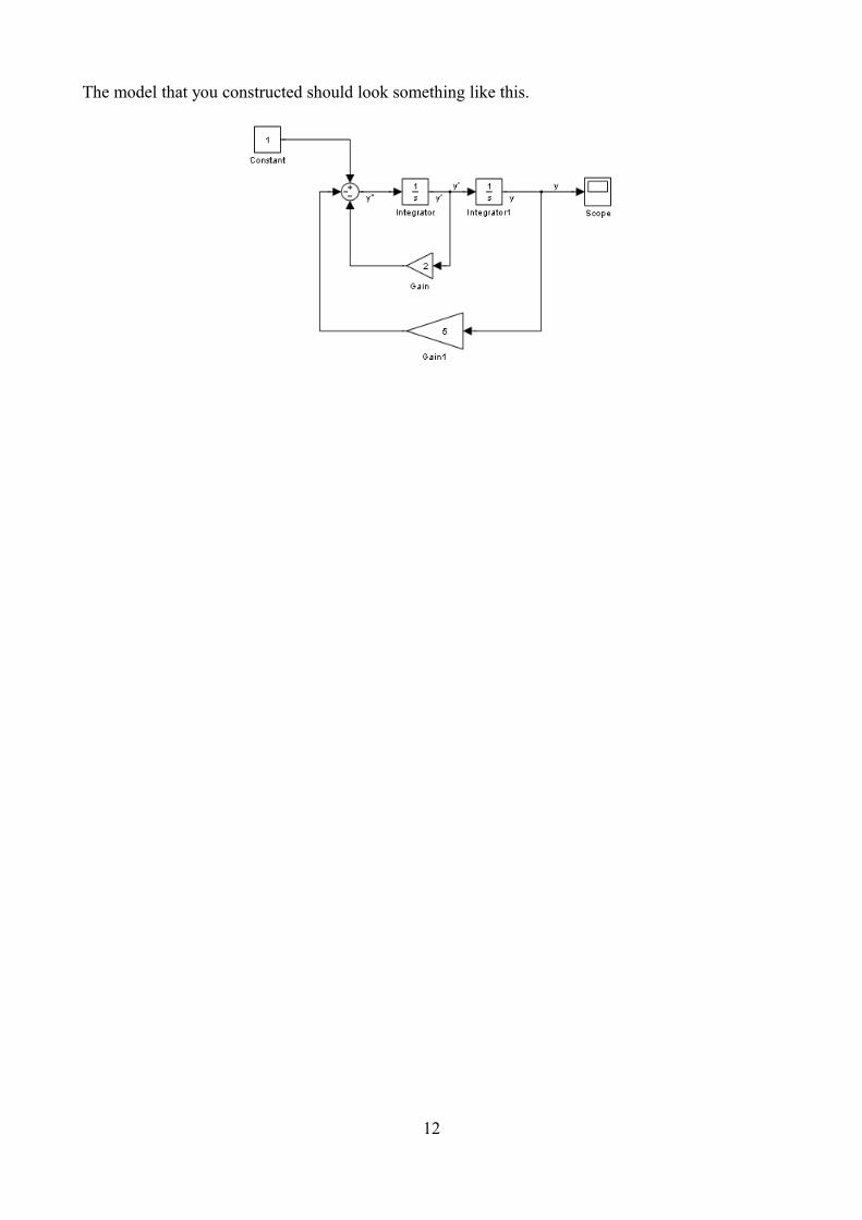
The model that you constructed should look something like this.

12

(b) Model the following set of differential equation.

[ xy]=[1

0][−2 −51 0 ][ x

y] (4)

x 0 = y 0=0

HintIt may help to first model the following equation.

U=CAU (5)

Where A and C are constants.

Then you set

C=[10] and A=[−2 −51 0 ]

And configure the multiplication to matrix multiplication.

Set max step size to 0.01

Save as ODE2.slx

Run the model

The output y should be the same as y in equation (1).PTO for an explanation of why this so ?

13

This is just a reformulated version of the equation in part (a). Take the equation from part (a).

d 2 y

dt 2=1−2 dy

dt−5y (2)

y=1−2 y−5y=1

Let x= y (6)

therefore x= y (7)

Substituting (6) and (7) into equation (2).x=1−2x−5y (8)

Equations (6) and (8) form a set of differential equationsx=1−2x−5y

y=x(9)

[ xy]=[1

0][−2 −51 0 ][ x

y] (10)

14

Exercise 3 (Bouncing Ball)(a) Build a Simulink model of a bouncing ball. Model the ball as a mass being dropped onto a spring damper system.

The equation of the system depends on the position of the ball.

If x 0x=−g (1)

If x < 0

x=− rm

x− km

x−g (2)

I suggest you start with m = 0.2, k = 1000 and r = 1. Try dropping the ball from a metre up.

(b) At the moment, the ball can go as low as it likes. In practice the ball cannot go lower than its radius. Modify the model so the ball cannot go lower than -0.02 metres.Hint, look at page 17 of the notes.

15

m

mg

x x

mg

k r