expansion of higher education, emplyment and …...working paper/document de travail 2013-45...
TRANSCRIPT
Working Paper/Document de travail 2013-45
Expansion of Higher Education, Employment and Wages: Evidence from the Russian Transition
by Natalia Kyui
2
Bank of Canada Working Paper 2013-45
December 2013
Expansion of Higher Education, Employment and Wages: Evidence from
the Russian Transition
by
Natalia Kyui
Canadian Economic Analysis Department Bank of Canada
Ottawa, Ontario, Canada K1A 0G9 [email protected]
Bank of Canada working papers are theoretical or empirical works-in-progress on subjects in economics and finance. The views expressed in this paper are those of the author.
No responsibility for them should be attributed to the Bank of Canada.
ISSN 1701-9397 © 2013 Bank of Canada

ii
Acknowledgements
I gratefully acknowledge the helpful discussions and kind support of Peter Arcidiacono, Paul Beaudry, Katya Kartashova, Guy Lacroix, Thomas Lemieux, Leigh L. Linden, Teodora Paligorova, Natalia Radtchenko, and Michel Sollogoub. I also thank audience participants at several conferences and seminars, where the earlier version of this paper was presented, such as EEA-ESEM’2011, JMA’2012, AEFP’2013, SCSE’2013, CLSRN-CEA’2013, ESPE’2013, EALE’2013, RECODE’2013, seminars at Laval University, Carleton University, Bank of Canada, and Centre d’Etudes de l’Emploi. For making these data available, I would like to thank the Russian Longitudinal Monitoring Survey Phase 2, funded by the USAID and NIH (R01-HD38700), Higher School of Economics and Pension Fund of Russia, and provided by the Carolina Population Center and Russian Institute of Sociology.
iii
Abstract
This paper analyzes the effects of an educational system expansion on labour market outcomes, drawing upon a 15-year natural experiment in the Russian Federation. Regional increases in student intake capacities in Russian universities, a result of educational reforms, provide a plausibly exogenous variation in access to higher education. Additionally, the gradual nature of this expansion allows for estimation of heterogeneous returns to education for individuals who successfully took advantage of increasing educational opportunities. Using simultaneous equations models and a non-parametric model with essential heterogeneity, the paper identifies strong positive returns to education in terms of employment and wages. Marginal returns to higher education are estimated to decline for lower levels of individual unobserved characteristics that positively influence higher education attainment. Finally, the returns to higher education are found to decrease for those who, as a result of the reforms, increasingly pursued higher education.
JEL classification: J24, I20 Bank classification: Labour markets; Development economics
Résumé
Cette étude analyse les effets d’un élargissement du système éducatif sur les salaires et les perspectives d’emploi des diplômés. Elle se fonde sur l’expérience naturelle de l’expansion de l’accès à l’enseignement supérieur dans la Fédération de Russie au cours des 15 dernières années. L’accroissement du nombre de places disponibles dans les universités au niveau régional, du fait des réformes de l’éducation, fournit une variation vraisemblablement exogène de l’accès à l’enseignement supérieur. Le caractère graduel de cet élargissement permet en outre d’estimer les rendements hétérogènes de l’éducation pour les individus qui ont bénéficié de l’amélioration de l’accès à l’enseignement supérieur. S’appuyant sur des résultats obtenus à l’aide de modèles à équations simultanées et d’un modèle non paramétrique à hétérogénéité essentielle, l’étude relève que les rendements de l’enseignement supérieur sont élevés sur le plan des salaires et de l’emploi. D’après les résultats de l’estimation, les rendements marginaux de l’enseignement supérieur diminuent lorsque les caractéristiques individuelles non observables qui influencent positivement la probabilité d’accéder à l’enseignement supérieur sont plus faibles. Enfin, il apparaît que les rendements de l’enseignement supérieur sont plus faibles pour ceux qui ont pu entreprendre des études supérieures à la suite des réformes que pour ceux qui poursuivaient des études supérieures indépendamment de l’élargissement du système éducatif.
Classification JEL : J24, I20 Classification de la Banque : Marchés du travail; Économie du développement
1 Introduction
This study quantifies the effects of an educational system expansion on labour market
outcomes and identifies the distribution of the returns to education, by exploring a nat-
ural experiment: a fifteen-year expansion of the higher education system in the Russian
Federation. During 1990–2005, the country, referred to here as Russia, saw a doubling in
student intake capacities in universities and, associated with this, a doubling in the number
of university graduates. This expansion, government-regulated to a large extent, provides
a plausibly exogenous variation in access to higher education at the regional level, and thus
allows identification of the returns to higher education in Russia. The gradual nature of
this increase in educational opportunities makes it possible to estimate returns to educa-
tion for individuals who were exposed to different degrees of higher education expansion
and who successfully took advantage of that. Finally, the paper evaluates the influence of
this expansion on labour market outcomes, namely on employment and wages.
Whether and to what extent additional education does increase an individual’s wages
and employment prospects, as well as generate a positive economic return for a country
– these are important questions both in the literature and for policy-makers. Such an
inquiry is especially relevant for those economies aiming to increase the educational level
of their population. Numerous studies show that workers with higher educational levels
have correspondingly higher wages. A current leading focus of the literature, however, is
identification of a causal effect of education on labour market outcomes, such as employ-
ment and wages, and thus its separation from potential selection biases.
This paper contributes primarily to the literature exploring changes in an educational
system for the identification of the causal effects of education on labour market outcomes,
in particular, on earnings.1 Within this literature are two main directions of research:
analysis of changes in compulsory schooling laws and of changes in access to education.
Using the first approach, researchers find a positive effect of compulsory schooling
legislation on educational attainment and future wages. Yet the magnitude of this effect
significantly varies among countries (see Angrist and Krueger (1991) for the United States,
Oreopoulos (2006b) for the United Kingdom, Pischke and von Wachter (2008) for Germany,
and Oreopoulos (2006a) for Canada). Because of the nature of compulsory schooling
legislation, this approach allows identification of the effects of additional years of secondary
schooling; these studies often use the total length of schooling as an educational variable,
and thus assume a constant return to a year of schooling for different educational levels.
The second approach, analysis of the changes in access to education on educational at-
tainment and labour market outcomes, encompasses studies focusing on the financial side
of the educational system (tuition fees and financial-aid policies: Kane and Rouse (1993),
Card and Lemieux (2001b), Arcidiacono (2005)), on the physical access to educational
institutions (distance to high schools and colleges, or their presence in the district: Card
1See Card (1999) and Belzil (2006) for an extensive analysis of other approaches to identifying thecausal effect of education on earnings.
2

(1995), Conneely and Uusitalo (1997)), and on the capacity of an educational system. This
last group of studies focuses on educational infrastructure and capacities. Duflo (2001) uses
the exposure to school construction in Indonesia, a major governmental project, to identify
its effects on educational attainment and future wages. Walker and Zhu (2008) analyze
the expansion of higher education in the United Kingdom during the period 1994–2006,
comparing the returns to education among different cohorts. They find no changes in the
returns to higher education for men, with one exception for the bottom quartile of the
distribution, and a significant rise in returns for women.
This is the first paper to our knowledge to identify the returns to higher education
by exploring the educational reforms in Russia, and the first to quantify the influence of
the expansion of the higher education system, caused by these reforms, on labour market
outcomes. Though several studies have analyzed the returns to education in Russia, they
treat educational attainment as exogenous, thus not correcting for the associated selection
bias (the exception being Cheidvasser and Benitez-Silva (2007), discussed below). Studies
conducted for the Soviet period2 show a small effect of education on earnings (however,
non-pecuniary returns might also have been important during this period).3 Gregory and
Kohlhase (1988) estimate the returns to education of a sample of Russian migrants to Israel;
they find positive and significant returns to completion of higher education for white-collar
workers (12.79%–22.38%) and insignificant returns for blue-collar workers. The work of
Cheidvasser and Benitez-Silva (2007) provides an analysis of the returns to education in
the Russian Federation for the years 1992–1999. Using a linear regression estimation of
Mincer’s equation, they show that the returns to an additional year of schooling are not
higher than 5% during the analyzed period. Belokonnaya et al. (2007), by estimation of
Mincer’s equation, show that the returns to higher education in 2005 are positive both
for men and women, though larger for female employees (27% and 40%, respectively, in
comparison to secondary education). Regarding the correction for the endogeneity of the
educational variable, Cheidvasser and Benitez-Silva (2007) use the instrumental variable
methodology, similarly to studies for other countries, by exploring the changes in compul-
sory schooling laws. Because the majority of the Russian population complete secondary
education, the current paper instead focuses on higher education attainment and the re-
turns to a higher education degree.
The major expansion of the Russian higher education system from 1990 to 2005, a result
of educational reforms, led Russia to become a leader, among OECD and G-20 countries,
2The Union of Soviet Socialist Republics (USSR), or Soviet Union, was a constitutionally socialist statethat existed in Eurasia from 1922 to 1991. The current study refers to this time as the Soviet period.
3Studies conducted with the data for the Soviet period (Gregory and Kohlhase (1988), Katz (1999), Oferand Vinokur (1992)) report different results on the returns to education, mainly due to the significantlydifferent population samples. The selectivity problem is thus important in these studies, but the limitedinformation on wages for this period does not provide more reliable and representative results. Nevertheless,it is not the purpose of the current study to comment on the evaluation of the returns to education in theSoviet period and after the collapse of the Soviet Union. These studies’ results are mentioned simply toprovide the reader with some background information about wages before the transition period.
3
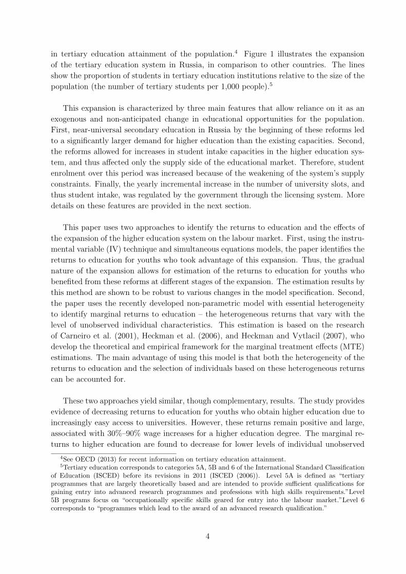
in tertiary education attainment of the population.4 Figure 1 illustrates the expansion
of the tertiary education system in Russia, in comparison to other countries. The lines
show the proportion of students in tertiary education institutions relative to the size of the
population (the number of tertiary students per 1,000 people).5
This expansion is characterized by three main features that allow reliance on it as an
exogenous and non-anticipated change in educational opportunities for the population.
First, near-universal secondary education in Russia by the beginning of these reforms led
to a significantly larger demand for higher education than the existing capacities. Second,
the reforms allowed for increases in student intake capacities in the higher education sys-
tem, and thus affected only the supply side of the educational market. Therefore, student
enrolment over this period was increased because of the weakening of the system’s supply
constraints. Finally, the yearly incremental increase in the number of university slots, and
thus student intake, was regulated by the government through the licensing system. More
details on these features are provided in the next section.
This paper uses two approaches to identify the returns to education and the effects of
the expansion of the higher education system on the labour market. First, using the instru-
mental variable (IV) technique and simultaneous equations models, the paper identifies the
returns to education for youths who took advantage of this expansion. Thus, the gradual
nature of the expansion allows for estimation of the returns to education for youths who
benefited from these reforms at different stages of the expansion. The estimation results by
this method are shown to be robust to various changes in the model specification. Second,
the paper uses the recently developed non-parametric model with essential heterogeneity
to identify marginal returns to education – the heterogeneous returns that vary with the
level of unobserved individual characteristics. This estimation is based on the research
of Carneiro et al. (2001), Heckman et al. (2006), and Heckman and Vytlacil (2007), who
develop the theoretical and empirical framework for the marginal treatment effects (MTE)
estimations. The main advantage of using this model is that both the heterogeneity of the
returns to education and the selection of individuals based on these heterogeneous returns
can be accounted for.
These two approaches yield similar, though complementary, results. The study provides
evidence of decreasing returns to education for youths who obtain higher education due to
increasingly easy access to universities. However, these returns remain positive and large,
associated with 30%–90% wage increases for a higher education degree. The marginal re-
turns to higher education are found to decrease for lower levels of individual unobserved
4See OECD (2013) for recent information on tertiary education attainment.5Tertiary education corresponds to categories 5A, 5B and 6 of the International Standard Classification
of Education (ISCED) before its revisions in 2011 (ISCED (2006)). Level 5A is defined as “tertiaryprogrammes that are largely theoretically based and are intended to provide sufficient qualifications forgaining entry into advanced research programmes and professions with high skills requirements.”Level5B programs focus on “occupationally specific skills geared for entry into the labour market.”Level 6corresponds to “programmes which lead to the award of an advanced research qualification.”
4
characteristics, which positively influence higher education attainment. Overall, the re-
sults suggest that this expansion of the higher education system has significantly increased
the wages of those who took advantage of its growing capacity. However, this increase is
smaller than the returns to education for those who would have pursued higher education
regardless.
The next two sections describe the institutional context of the Russian educational re-
forms and the data. Section 4 discusses the estimation results using the IV approach of
the returns to education and provides several robustness checks. Section 5 analyzes the
heterogeneity in the returns to education, using a non-parametric approach. Section 6
concludes. The Technical Appendix provides details on the estimation of the simultaneous
equations models and the model with essential heterogeneity.
2 Institutional Context
This section describes in detail the educational system in Russia and the recent reforms
on which this paper focuses. The Russian system, inherited from the Soviet period, con-
sists of four levels: primary and general education (8 years at schools); secondary education
(an additional 2 years at general or specialized schools); tertiary education (2-6 years at
a post-secondary institution); and post-graduate education (3-6 years at universities with
PhD programs). Tertiary education is in turn divided into two streams that are not con-
secutive levels. The first, corresponding to ISCED level 5B, is post-secondary technical or
vocational education; it consists of 2-3 years of study at technical or specialized schools,
such as military, medical or musical. The second type, corresponding to ISCED level 5A, is
higher education; it requires 4-6 years of studies at universities after secondary education.
This last educational level is the main focus of the current study.
During the Soviet period, the government completely regulated the educational sector.
Education, both secondary and tertiary, was financed from the country’s budget and was
free for students (thus referred to here as state-subsidized education).6 One of the main
achievements of the educational policy during the Soviet period was a large expansion of
secondary education: the share of the population 15 years and older without a secondary
education degree decreased from almost 61% in 1959 to less than 20% in 1989.7 As a
result, the share of the Russian working-age population with at least a secondary level of
6The development of education became a priority for the Russian government at the beginning of thetwentieth century, and even now education is a high priority for the country. After the Revolution of 1917,the Russian government started major reforms in the educational sector in order to provide universal publiceducation (Lukov (2005)). The tuition fees in secondary and especially tertiary education were completelyeliminated by 1954. The 1958 law introducing compulsory 8-year schooling determined some generalprinciples of the connections between work and education, framing vocational schooling and prioritizingnot only education for youths, but also for experienced workers going back to school.
7Cited numbers are from the Russian census of 1959 and 1989. Universal secondary education was themain educational priority of the Soviet government from 1965 on.
5
education increased to more than 90% and placed Russia among the countries with the
highest level of secondary education attainment of population in the world.8 Regarding
tertiary education, the Soviet government determined the number of slots according to
the economy’s predicted needs for the following years. The number of slots in tertiary
education was limited and fully state-subsidized. Aspiring students were admitted on a
competitive basis and admission tests selected high-ability candidates. The growing access
to secondary education increased the number of applicants for tertiary education programs,
especially to universities.
With the beginning of the transition, in 1992, the Russian government passed the law
“On Education,”marking the start of major changes in the tertiary education system. The
most important amendment introduced tuition-based, in addition to state-subsidized, ter-
tiary education. First, the government authorized the creation and operation of non-public
(private) tertiary education institutions with the proviso that they be run as not-for-profit
organizations, albeit providing educational services to the population on a full-tuition ba-
sis. Second, the government authorized public tertiary education institutions to admit
students on a full-tuition basis in addition to the state-subsidized slots, which continue to
be financed by the government. These changes on the supply side, along with a large and
persistent demand for tertiary education (primarily due to universal secondary education
and perceived positive returns to tertiary education), led to a major expansion of the ter-
tiary education system in Russia. During the following decade, the number of slots in the
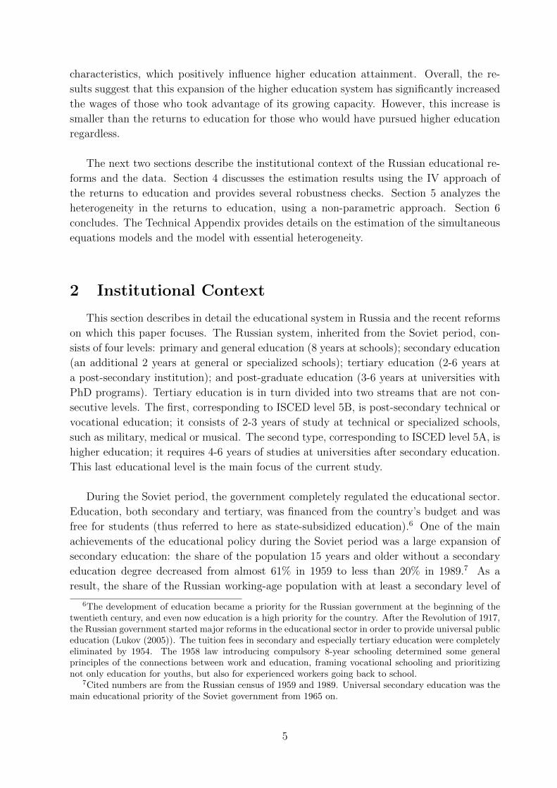
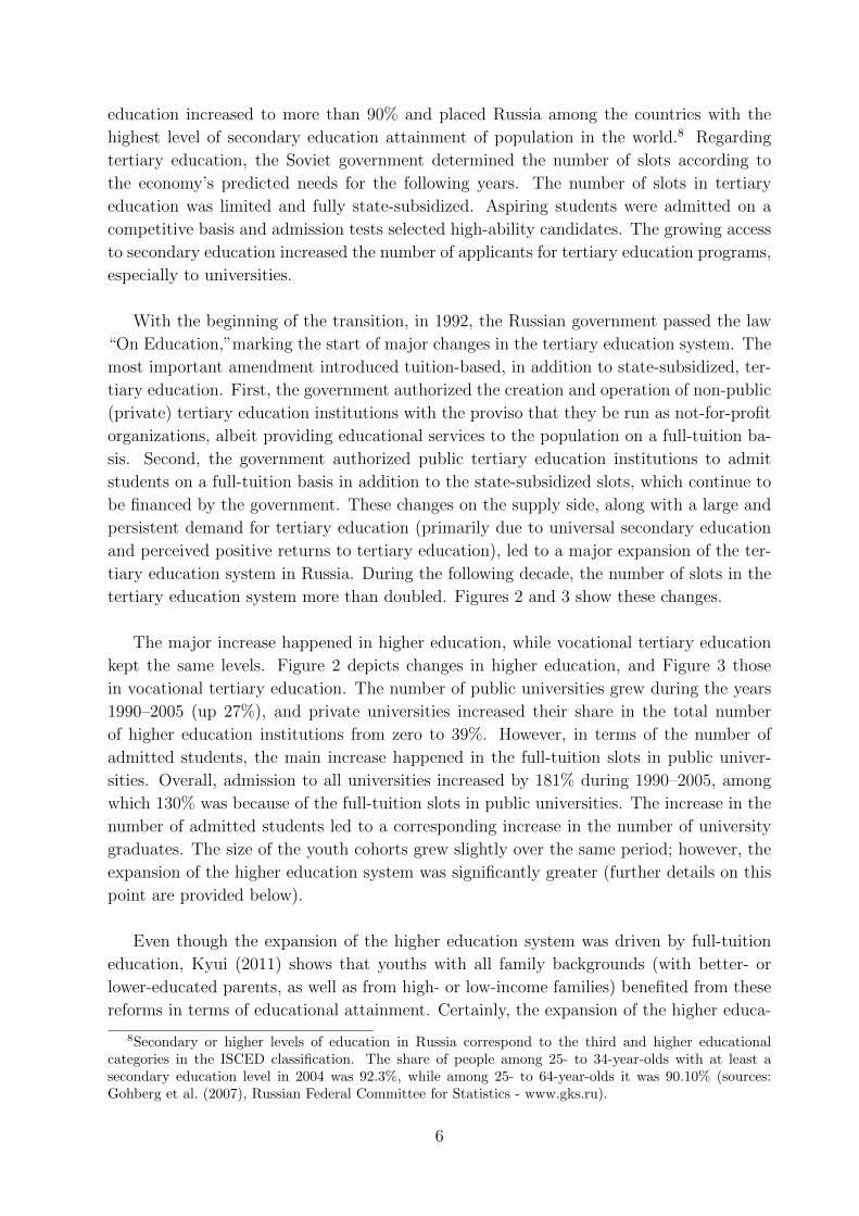
tertiary education system more than doubled. Figures 2 and 3 show these changes.
The major increase happened in higher education, while vocational tertiary education
kept the same levels. Figure 2 depicts changes in higher education, and Figure 3 those
in vocational tertiary education. The number of public universities grew during the years
1990–2005 (up 27%), and private universities increased their share in the total number
of higher education institutions from zero to 39%. However, in terms of the number of
admitted students, the main increase happened in the full-tuition slots in public univer-
sities. Overall, admission to all universities increased by 181% during 1990–2005, among
which 130% was because of the full-tuition slots in public universities. The increase in the
number of admitted students led to a corresponding increase in the number of university
graduates. The size of the youth cohorts grew slightly over the same period; however, the
expansion of the higher education system was significantly greater (further details on this
point are provided below).
Even though the expansion of the higher education system was driven by full-tuition
education, Kyui (2011) shows that youths with all family backgrounds (with better- or
lower-educated parents, as well as from high- or low-income families) benefited from these
reforms in terms of educational attainment. Certainly, the expansion of the higher educa-
8Secondary or higher levels of education in Russia correspond to the third and higher educationalcategories in the ISCED classification. The share of people among 25- to 34-year-olds with at least asecondary education level in 2004 was 92.3%, while among 25- to 64-year-olds it was 90.10% (sources:Gohberg et al. (2007), Russian Federal Committee for Statistics - www.gks.ru).
6
tion system is limited by the demand for higher education; in other words, by the number
of youths willing to enter the higher education institutions. Until recent years, admission
selection processes were locally organized by educational institutions, which is why the
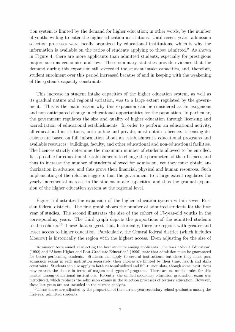
information is available on the ratios of students applying to those admitted.9 As shown
in Figure 4, there are more applicants than admitted students, especially for prestigious
majors such as economics and law. These summary statistics provide evidence that the
demand during this expansion still exceeded the student intake capacities, and, therefore,
student enrolment over this period increased because of and in keeping with the weakening
of the system’s capacity constraints.
This increase in student intake capacities of the higher education system, as well as
its gradual nature and regional variation, was to a large extent regulated by the govern-
ment. This is the main reason why this expansion can be considered as an exogenous
and non-anticipated change in educational opportunities for the population. In particular,
the government regulates the size and quality of higher education through licensing and
accreditation of educational establishments. In order to perform an educational activity,
all educational institutions, both public and private, must obtain a licence. Licensing de-
cisions are based on full information about an establishment’s educational programs and
available resources: buildings, faculty, and other educational and non-educational facilities.
The licences strictly determine the maximum number of students allowed to be enrolled.
It is possible for educational establishments to change the parameters of their licences and
thus to increase the number of students allowed for admission, yet they must obtain au-
thorization in advance, and thus prove their financial, physical and human resources. Such
implementing of the reforms suggests that the government to a large extent regulates the
yearly incremental increase in the student intake capacities, and thus the gradual expan-
sion of the higher education system at the regional level.
Figure 5 illustrates the expansion of the higher education system within seven Rus-
sian federal districts. The first graph shows the number of admitted students for the first
year of studies. The second illustrates the size of the cohort of 17-year-old youths in the
corresponding years. The third graph depicts the proportions of the admitted students
to the cohorts.10 These data suggest that, historically, there are regions with greater and
lesser access to higher education. Particularly, the Central federal district (which includes
Moscow) is historically the region with the highest access. Even adjusting for the size of
9Admission tests aimed at selecting the best students among applicants. The laws “About Education”(1992) and “About Higher and Post-Graduate Education” (1996) state that admission must be guaranteedfor better-performing students. Students can apply to several institutions, but since they must passadmission exams in each institution separately, their choices are limited by their time, health and skillsconstraints. Students can also apply to both state-subsidized and full-tuition slots, though some institutionsmay restrict the choice in terms of majors and types of programs. There are no unified rules for thismatter among educational institutions. Recently, the unified secondary education graduation exam wasintroduced, which replaces the admission exams in the selection processes of tertiary education. However,these last years are not included in the current analysis.
10These shares are adjusted by the proportion of the current-year secondary school graduates among thefirst-year admitted students.
7
the population, these differences in the capacity of the higher education system are still
important among regions, and thus the expansion of higher education varied among re-
gions. The regions with the highest number of slots in the higher education system have
kept their leadership positions. Therefore, the varying educational resources in the regions
at the beginning of transition, along with governmental control over licensing, are a main
explanation of these regional differences in the trajectories of expansion. Overall, these
factors strongly suggest that the yearly changes in access to higher education within re-
gions were plausibly exogenous and non-anticipated for youths and their families.
3 Data Description
Data are taken from the Russian Longitudinal Monitoring Survey (RLMS), a series of
nationally representative surveys designed to monitor the effects of Russian reforms on the
health and economic welfare of households and individuals in the Russian Federation. The
RLMS data are described in Swafford et al. (1999a,b).
The samples of 24- to 47-year-olds, interviewed in the years 2000–2008, are used as
the repeated cross-sections for this analysis. Those observed were making decisions about
tertiary education attainment when they were 17 years old, in 1970–2001, thus before and
during the expansion of tertiary education in Russia.11 Overall, there are 41,585 observa-
tions; among them, 10,288 are unemployed and 31,297 are employed. However, among the
employed population the wages are observed only in 91.5% of cases. Thus, the final sample
used for the analysis consists of 28,622 employed and 10,288 unemployed people.
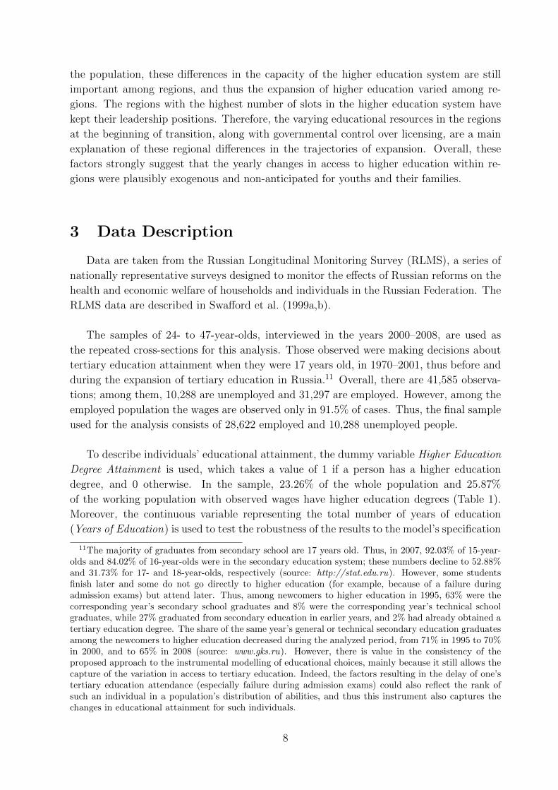
To describe individuals’ educational attainment, the dummy variable Higher Education
Degree Attainment is used, which takes a value of 1 if a person has a higher education
degree, and 0 otherwise. In the sample, 23.26% of the whole population and 25.87%
of the working population with observed wages have higher education degrees (Table 1).
Moreover, the continuous variable representing the total number of years of education
(Years of Education) is used to test the robustness of the results to the model’s specification
11The majority of graduates from secondary school are 17 years old. Thus, in 2007, 92.03% of 15-year-olds and 84.02% of 16-year-olds were in the secondary education system; these numbers decline to 52.88%and 31.73% for 17- and 18-year-olds, respectively (source: http://stat.edu.ru). However, some studentsfinish later and some do not go directly to higher education (for example, because of a failure duringadmission exams) but attend later. Thus, among newcomers to higher education in 1995, 63% were thecorresponding year’s secondary school graduates and 8% were the corresponding year’s technical schoolgraduates, while 27% graduated from secondary education in earlier years, and 2% had already obtained atertiary education degree. The share of the same year’s general or technical secondary education graduatesamong the newcomers to higher education decreased during the analyzed period, from 71% in 1995 to 70%in 2000, and to 65% in 2008 (source: www.gks.ru). However, there is value in the consistency of theproposed approach to the instrumental modelling of educational choices, mainly because it still allows thecapture of the variation in access to tertiary education. Indeed, the factors resulting in the delay of one’stertiary education attendance (especially failure during admission exams) could also reflect the rank ofsuch an individual in a population’s distribution of abilities, and thus this instrument also captures thechanges in educational attainment for such individuals.
8

(see section 4.4 for details).
Table 1: Higher Education Degree Attainment, 24- to 47-year-olds, 2000–2008
Higher Education Employed, 24–47-y.o. Employed Unemployed ALL
Attainment with Observed Wages 24–47-y.o. 24–47-y.o. 24–47-y.o.
0 74.13% 74.23% 84.37% 76.74%
1 25.87% 25.77% 15.63% 23.26%
Total 28,622 31,297 10,288 41,585
Sources: RLMS, 2000–2008, author’s calculations
An individual who self-identifies as having a job is considered to be employed. The in-
dividual’s average monthly income from working activity is used as a measure of wages.12
Wages are adjusted for inflation by the consumer price index. In order to account for
the regional differences in prices, and to make regional wages comparable, wages are ad-
ditionally corrected by the regional price of a standard product set. The exposure of an
individual to the expansion of the higher education system is identified by the year when
the individual turned 17 years old (thus graduating from secondary school and deciding
on further tertiary education) and by the federal district of residency. Along with the
control for year and federal district fixed effects, the changes in the capacity of the higher
education system provide a plausibly exogenous variation in access to higher education.
4 Returns to Education:
Local Average Treatment Effects
This section discusses the identification and estimation of the returns to higher ed-
ucation and the effects of the educational system expansion on employment and wages.
Variation in the opportunities of obtaining higher education (i.e., variation in the number
of available slots in universities) is used as the instrument for higher education attainment.
First, the section describes the explanatory power of this instrument. Second, it shows the
estimation results for the returns to education in terms of employment and wages. Finally,
several robustness checks are described. Section 5 discusses the estimation of heterogeneity
in the returns to education.
4.1 Instrument choice and characteristics
Table 2 reports the results for the “first-stage” equation: the influence of the changes
in the educational system (increasing number of slots) on higher education attainment.
12Information on the number of hours worked contains many missing and out-of-normal-range values;for this reason, the hourly wage is not used for the estimations.
9
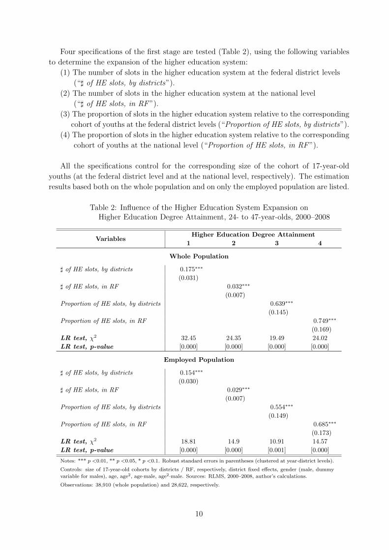
Four specifications of the first stage are tested (Table 2), using the following variables
to determine the expansion of the higher education system:
(1) The number of slots in the higher education system at the federal district levels
(“] of HE slots, by districts”).
(2) The number of slots in the higher education system at the national level
(“] of HE slots, in RF”).
(3) The proportion of slots in the higher education system relative to the corresponding
cohort of youths at the federal district levels (“Proportion of HE slots, by districts”).
(4) The proportion of slots in the higher education system relative to the corresponding
cohort of youths at the national level (“Proportion of HE slots, in RF”).
All the specifications control for the corresponding size of the cohort of 17-year-old
youths (at the federal district level and at the national level, respectively). The estimation
results based both on the whole population and on only the employed population are listed.
Table 2: Influence of the Higher Education System Expansion onHigher Education Degree Attainment, 24- to 47-year-olds, 2000–2008
VariablesHigher Education Degree Attainment
1 2 3 4
Whole Population
] of HE slots, by districts 0.175∗∗∗
(0.031)
] of HE slots, in RF 0.032∗∗∗
(0.007)
Proportion of HE slots, by districts 0.639∗∗∗
(0.145)
Proportion of HE slots, in RF 0.749∗∗∗
(0.169)
LR test, χ2 32.45 24.35 19.49 24.02
LR test, p-value [0.000] [0.000] [0.000] [0.000]
Employed Population
] of HE slots, by districts 0.154∗∗∗
(0.030)
] of HE slots, in RF 0.029∗∗∗
(0.007)
Proportion of HE slots, by districts 0.554∗∗∗
(0.149)
Proportion of HE slots, in RF 0.685∗∗∗
(0.173)
LR test, χ2 18.81 14.9 10.91 14.57
LR test, p-value [0.000] [0.000] [0.001] [0.000]
Notes: *** p <0.01, ** p <0.05, * p <0.1. Robust standard errors in parentheses (clustered at year·district levels).
Controls: size of 17-year-old cohorts by districts / RF, respectively, district fixed effects, gender (male, dummy
variable for males), age, age2, age·male, age2·male. Sources: RLMS, 2000–2008, author’s calculations.
Observations: 38,910 (whole population) and 28,622, respectively.
10
Statistics for the test on exclusion of the instruments from the first-stage equation sug-
gest that the variables describing the number of slots have a higher explanatory power than
those describing the ratio of the number of slots to the size of the corresponding youth
cohorts. Moreover, the variables at federal district levels have a higher explanatory power
than those at the Russian level. This result was expected, and it is due both to the addi-
tional variation in the size of the higher education system and to the different patterns of
its expansion among regions. Therefore, for further estimations, the number of slots in the
higher education at federal district levels is used as the instrument for the higher education
degree attainment (with a control for the size of 17-year-old cohorts at the federal district
level). This variable passes the instrument-weakness test (see also section 4.4 for details
using the continuous variable to describe educational attainment).13
The main potential problem with this instrument is the fact that it is perfectly corre-
lated with region-cohort effects, which means that there are no variations of the instrument
within a group of people born in one year and living in the same federal district. Therefore,
it is necessary to assume that if there were any unobserved changes affecting wages, they
were not correlated with the tertiary education system expansion within the regions over
time. In order to account for that, several steps are performed. First, all the specifications
control for the year and region fixed effects, thus capturing the unobserved variations of
other characteristics by regions and over the analyzed period. However, it is still necessary
to assume that there were no changes, affecting wages and correlating with the educational
system expansion within regions, other than those captured by the fixed effects for years
and federal districts. Therefore, additional controls for the cohort year-of-birth fixed effects
and region-specific linear cohort trends are included when performing robustness checks.
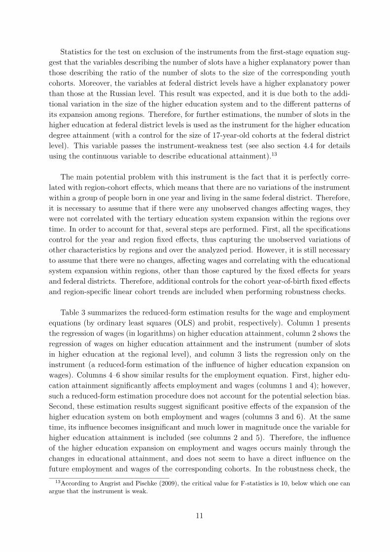
Table 3 summarizes the reduced-form estimation results for the wage and employment
equations (by ordinary least squares (OLS) and probit, respectively). Column 1 presents
the regression of wages (in logarithms) on higher education attainment, column 2 shows the
regression of wages on higher education attainment and the instrument (number of slots
in higher education at the regional level), and column 3 lists the regression only on the
instrument (a reduced-form estimation of the influence of higher education expansion on
wages). Columns 4–6 show similar results for the employment equation. First, higher edu-
cation attainment significantly affects employment and wages (columns 1 and 4); however,
such a reduced-form estimation procedure does not account for the potential selection bias.
Second, these estimation results suggest significant positive effects of the expansion of the
higher education system on both employment and wages (columns 3 and 6). At the same
time, its influence becomes insignificant and much lower in magnitude once the variable for
higher education attainment is included (see columns 2 and 5). Therefore, the influence
of the higher education expansion on employment and wages occurs mainly through the
changes in educational attainment, and does not seem to have a direct influence on the
future employment and wages of the corresponding cohorts. In the robustness check, the
13According to Angrist and Pischke (2009), the critical value for F-statistics is 10, below which one canargue that the instrument is weak.
11
potential equilibrium effects of the higher education expansion on wages are also tested
and discussed (see section 4.4 for more details); here, the main focus is on the individual
returns to education.
Table 3: Reduced-Form Estimations: Wages and Employment,24- to 47-year-olds, Employed and Whole Population, 2000–2008
Variablesln(Wage), by OLS Employment, by probit
1 2 3 4 5 6
HE degree* 0.457∗∗∗ 0.457∗∗∗ 0.389∗∗∗ 0.388∗∗∗
(0.011) (0.011) (0.021) (0.021)
] of HE slots, by districts 0.021 0.052∗∗ 0.038 0.065∗∗
(0.021) (0.023) (0.028) (0.027)
Observations 28,622 28,622 28,622 38,910 38,910 38,910
Notes: *** p <0.01, ** p <0.05, * p <0.1. Robust standard errors in parentheses (clustered at year·district levels).
Controls: year and federal district fixed effects, gender (male), age, age2, age·male, age2·male, size of 17-year-old cohorts
by districts, regional unemployment rates for the employment equation.
Sources: RLMS, 2000–2008, author’s calculations. The wage equation is estimated for the employed population using
the OLS method, and the employment equation is estimated for the whole population using the probit model.
Observations: 28,622 (employed population) and 38,910 (whole population).
4.2 Returns to education: wages
The joint model of higher education degree attainment and wages is estimated using
the maximum likelihood method; the estimation procedure is described in section 1 of the
Technical Appendix. The above-mentioned expansion of the higher education system at
Russian regional levels is used as the instrument for higher education degree attainment.
This simultaneous equations model allows for control of the endogeneity of educational
attainment, and thus of the self-selection of individuals into higher education. Table 4 lists
the estimation results.
Estimated returns to education, using this joint model of higher education degree at-
tainment and wages, are higher than those obtained by OLS (Table 3). Returns to a
complete higher education degree are estimated at the level of 76%. The correlation be-
tween unobserved terms in educational attainment and the wage equation is estimated to
be negative and significant. IV estimations of the returns to education report an increase in
wages for those who obtained an education degree because of the instrument variation and
who would not otherwise have received it (Angrist et al. (1996)). Therefore, the estimated
returns to education represent the local average treatment effect: returns to education
for those who have obtained a higher education degree because of the growing access to
universities. The results suggest that individuals who benefited from the expansion of the
higher education system in terms of educational attainment have also gained in terms of
wages.
12
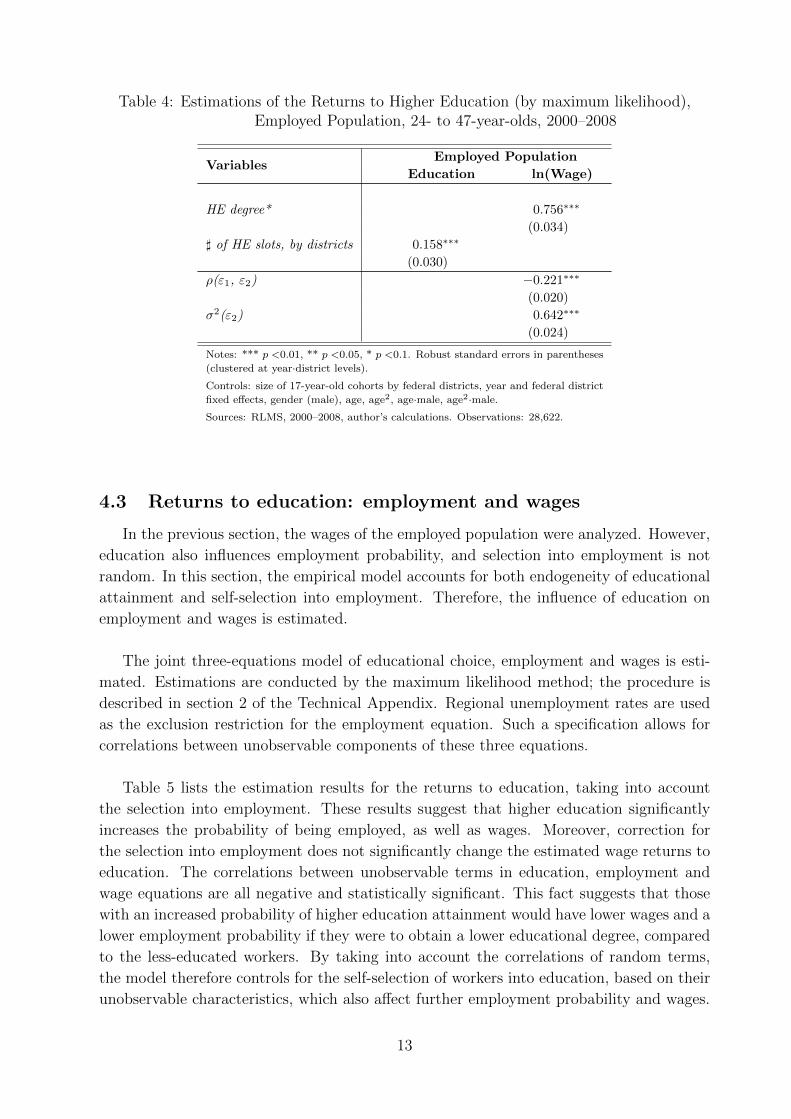
Table 4: Estimations of the Returns to Higher Education (by maximum likelihood),Employed Population, 24- to 47-year-olds, 2000–2008
VariablesEmployed Population
Education ln(Wage)
HE degree* 0.756∗∗∗
(0.034)
] of HE slots, by districts 0.158∗∗∗
(0.030)
ρ(ε1, ε2) −0.221∗∗∗
(0.020)
σ2(ε2) 0.642∗∗∗
(0.024)
Notes: *** p <0.01, ** p <0.05, * p <0.1. Robust standard errors in parentheses
(clustered at year·district levels).
Controls: size of 17-year-old cohorts by federal districts, year and federal district
fixed effects, gender (male), age, age2, age·male, age2·male.
Sources: RLMS, 2000–2008, author’s calculations. Observations: 28,622.
4.3 Returns to education: employment and wages
In the previous section, the wages of the employed population were analyzed. However,
education also influences employment probability, and selection into employment is not
random. In this section, the empirical model accounts for both endogeneity of educational
attainment and self-selection into employment. Therefore, the influence of education on
employment and wages is estimated.
The joint three-equations model of educational choice, employment and wages is esti-
mated. Estimations are conducted by the maximum likelihood method; the procedure is
described in section 2 of the Technical Appendix. Regional unemployment rates are used
as the exclusion restriction for the employment equation. Such a specification allows for
correlations between unobservable components of these three equations.
Table 5 lists the estimation results for the returns to education, taking into account
the selection into employment. These results suggest that higher education significantly
increases the probability of being employed, as well as wages. Moreover, correction for
the selection into employment does not significantly change the estimated wage returns to
education. The correlations between unobservable terms in education, employment and
wage equations are all negative and statistically significant. This fact suggests that those
with an increased probability of higher education attainment would have lower wages and a
lower employment probability if they were to obtain a lower educational degree, compared
to the less-educated workers. By taking into account the correlations of random terms,
the model therefore controls for the self-selection of workers into education, based on their
unobservable characteristics, which also affect further employment probability and wages.
13
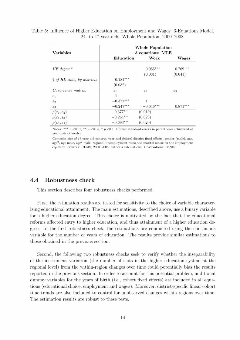
Table 5: Influence of Higher Education on Employment and Wages: 3-Equations Model,24- to 47-year-olds, Whole Population, 2000–2008
Variables
Whole Population
3 equations: MLE
Education Work Wages
HE degree* 0.955∗∗∗ 0.769∗∗∗
(0.031) (0.041)
] of HE slots, by districts 0.181∗∗∗
(0.032)
Covariance matrix: ε1 ε2 ε3ε1 1
ε2 −0.377∗∗∗ 1
ε3 −0.247∗∗∗ −0.646∗∗∗ 0.871∗∗∗
ρ(ε1, ε2) −0.377∗∗∗ (0.019)
ρ(ε1, ε3) −0.264∗∗∗ (0.023)
ρ(ε2, ε3) −0.693∗∗∗ (0.020)
Notes: *** p <0.01, ** p <0.05, * p <0.1. Robust standard errors in parentheses (clustered at
year·district levels).
Controls: size of 17-year-old cohorts, year and federal district fixed effects, gender (male), age,
age2, age·male, age2·male; regional unemployment rates and marital status in the employment
equation. Sources: RLMS, 2000–2008, author’s calculations. Observations: 38,910.
4.4 Robustness check
This section describes four robustness checks performed.
First, the estimation results are tested for sensitivity to the choice of variable character-
izing educational attainment. The main estimations, described above, use a binary variable
for a higher education degree. This choice is motivated by the fact that the educational
reforms affected entry to higher education, and thus attainment of a higher education de-
gree. In the first robustness check, the estimations are conducted using the continuous
variable for the number of years of education. The results provide similar estimations to
those obtained in the previous section.
Second, the following two robustness checks seek to verify whether the inseparability
of the instrument variation (the number of slots in the higher education system at the
regional level) from the within-region changes over time could potentially bias the results
reported in the previous section. In order to account for this potential problem, additional
dummy variables for the years of birth (i.e., cohort fixed effects) are included in all equa-
tions (educational choice, employment and wages). Moreover, district-specific linear cohort
time trends are also included to control for unobserved changes within regions over time.
The estimation results are robust to these tests.
14
Third, the interaction terms of the instrument with other individual characteristics are
included in the first equation for educational attainment, particularly in interactions with
gender and parental educational background (concurrently, the gender and parental edu-
cation variables are also included in all other equations).
The fourth and final robustness test aims to evaluate the importance in the labour
market of possible equilibrium effects of the expansion of the higher education system. For
instance, an increasing supply of new university graduates could have an effect on all other
university degree holders in the labour market, namely, a potential decrease in their wages.
Certainly, the cohorts’ effects on equilibrium of the labour market are accounted for by
introducing the year-of-birth dummy variables in the second robustness test. Additionally,
changes in the returns to education are evaluated during the analyzed period.
4.4.1 Continuous educational variable
This section reports the estimation results, using a continuous variable for the number
of years of education instead of a binary variable for higher education degree attainment.
In particular, the variable Years of Education describes the number of years of schooling
and ranges from 9 to 15 years. Higher education degree attainment corresponds to 15 years
of total schooling; 13 and 14 years of schooling correspond to complete/incomplete voca-
tional education or to incomplete higher education; and 10 years of schooling correspond
to secondary school completion.
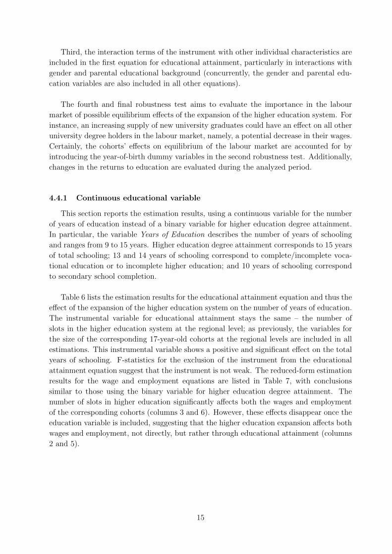
Table 6 lists the estimation results for the educational attainment equation and thus the
effect of the expansion of the higher education system on the number of years of education.
The instrumental variable for educational attainment stays the same – the number of
slots in the higher education system at the regional level; as previously, the variables for
the size of the corresponding 17-year-old cohorts at the regional levels are included in all
estimations. This instrumental variable shows a positive and significant effect on the total
years of schooling. F-statistics for the exclusion of the instrument from the educational
attainment equation suggest that the instrument is not weak. The reduced-form estimation
results for the wage and employment equations are listed in Table 7, with conclusions
similar to those using the binary variable for higher education degree attainment. The
number of slots in higher education significantly affects both the wages and employment
of the corresponding cohorts (columns 3 and 6). However, these effects disappear once the
education variable is included, suggesting that the higher education expansion affects both
wages and employment, not directly, but rather through educational attainment (columns
2 and 5).
15
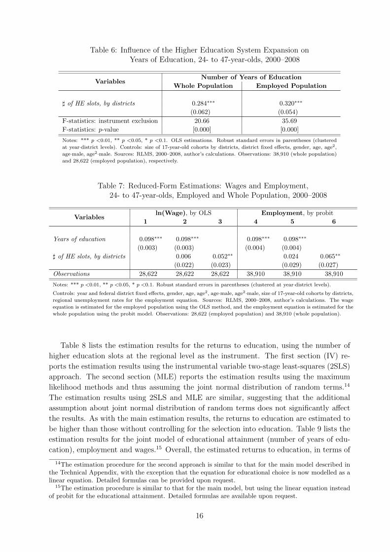
Table 6: Influence of the Higher Education System Expansion onYears of Education, 24- to 47-year-olds, 2000–2008
VariablesNumber of Years of Education
Whole Population Employed Population
] of HE slots, by districts 0.284∗∗∗ 0.320∗∗∗
(0.062) (0.054)
F-statistics: instrument exclusion 20.66 35.69
F-statistics: p-value [0.000] [0.000]
Notes: *** p <0.01, ** p <0.05, * p <0.1. OLS estimations. Robust standard errors in parentheses (clustered
at year·district levels). Controls: size of 17-year-old cohorts by districts, district fixed effects, gender, age, age2,
age·male, age2·male. Sources: RLMS, 2000–2008, author’s calculations. Observations: 38,910 (whole population)
and 28,622 (employed population), respectively.
Table 7: Reduced-Form Estimations: Wages and Employment,24- to 47-year-olds, Employed and Whole Population, 2000–2008
Variablesln(Wage), by OLS Employment, by probit
1 2 3 4 5 6
Years of education 0.098∗∗∗ 0.098∗∗∗ 0.098∗∗∗ 0.098∗∗∗
(0.003) (0.003) (0.004) (0.004)
] of HE slots, by districts 0.006 0.052∗∗ 0.024 0.065∗∗
(0.022) (0.023) (0.029) (0.027)
Observations 28,622 28,622 28,622 38,910 38,910 38,910
Notes: *** p <0.01, ** p <0.05, * p <0.1. Robust standard errors in parentheses (clustered at year·district levels).
Controls: year and federal district fixed effects, gender, age, age2, age·male, age2·male, size of 17-year-old cohorts by districts,
regional unemployment rates for the employment equation. Sources: RLMS, 2000–2008, author’s calculations. The wage
equation is estimated for the employed population using the OLS method, and the employment equation is estimated for the
whole population using the probit model. Observations: 28,622 (employed population) and 38,910 (whole population).
Table 8 lists the estimation results for the returns to education, using the number of
higher education slots at the regional level as the instrument. The first section (IV) re-
ports the estimation results using the instrumental variable two-stage least-squares (2SLS)
approach. The second section (MLE) reports the estimation results using the maximum
likelihood methods and thus assuming the joint normal distribution of random terms.14
The estimation results using 2SLS and MLE are similar, suggesting that the additional
assumption about joint normal distribution of random terms does not significantly affect
the results. As with the main estimation results, the returns to education are estimated to
be higher than those without controlling for the selection into education. Table 9 lists the
estimation results for the joint model of educational attainment (number of years of edu-
cation), employment and wages.15 Overall, the estimated returns to education, in terms of
14The estimation procedure for the second approach is similar to that for the main model described inthe Technical Appendix, with the exception that the equation for educational choice is now modelled as alinear equation. Detailed formulas can be provided upon request.
15The estimation procedure is similar to that for the main model, but using the linear equation insteadof probit for the educational attainment. Detailed formulas are available upon request.
16

employment and wages, are found to be of the same magnitude as in the main estimations
(note that higher education degree attainment corresponds to five years of studies). There-
fore, the estimation results are robust to the form of the variable describing educational
attainment.
Table 8: Estimations of the Returns to Higher Education (by IV and Maximum Likeli-hood), Employed Population, 24- to 47-year-olds, 2000–2008
Variables
Employed Population
IV MLE
Education ln(Wage) Education ln(Wage)
Years of education 0.116∗∗∗ 0.115∗∗∗
(0.070) (0.006)
] of HE slots, by districts 0.320∗∗∗ 0.319∗∗∗
(0.054) (0.054)
ρ(ε1, ε2) −0.048∗∗∗
(0.016)
σ2(ε1), σ2(ε2) 4.878∗∗∗ 0.619∗∗∗
(0.030) (0.023)
Notes: *** p <0.01, ** p <0.05, * p <0.1. Robust standard errors in parentheses (clustered at year·district levels).
Estimations are conducted using IV and maximum likelihood methods, respectively.
Controls: size of 17-year-old cohorts by federal districts, year and federal district fixed effects, gender, age, age2,
age·male, age2·male. Sources: RLMS, 2000–2008, author’s calculations. Observations: 28,622.
Table 9: Influence of Higher Education on Employment and Wages: 3-Equations Model,24- to 47-year-olds, Whole Population, 2000–2008
Variables
Whole Population
3 equations: MLE
Education Work Wages
Years of education 0.171∗∗∗ 0.165∗∗∗
(0.028) (0.028)
] of HE slots, by districts 0.274∗∗∗
(0.053)
Covariance matrix: ε1 ε2 ε3ε1 4.878∗∗∗
ε2 −0.415∗∗∗ 1
ε3 −0.463∗∗∗ −0.587∗∗∗ 0.827∗∗∗
ρ(ε1, ε2) −0.188∗∗∗ (0.063)
ρ(ε1, ε3) −0.231∗∗∗ (0.063)
ρ(ε2, ε3) −0.646∗∗∗ (0.037)
Notes: *** p <0.01, ** p <0.05, * p <0.1. Robust standard errors in parentheses (clustered at
year·district levels). Controls: size of 17-year-old cohorts by federal districts, year and federal district
fixed effects, gender, age, age2, age·male, age2·male; regional unemployment rates and marital status
in the employment equation. Sources: RLMS, 2000–2008, author’s calculations. Observations:
38,910.
17
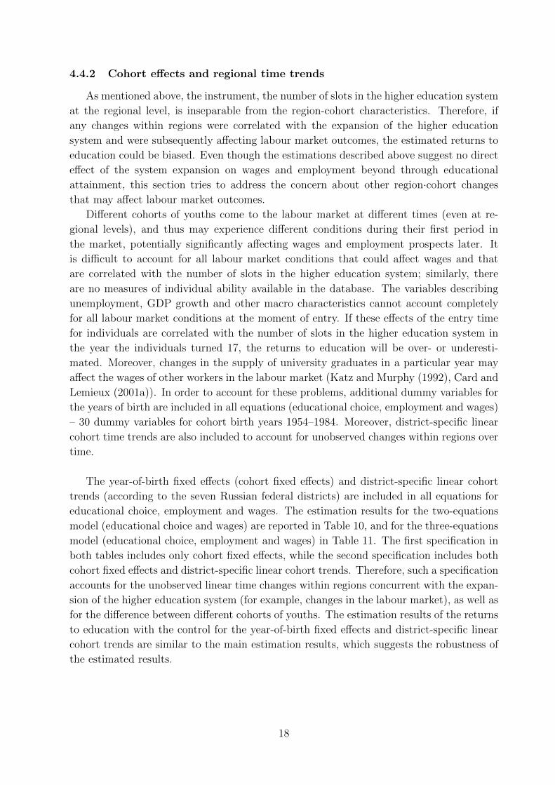
4.4.2 Cohort effects and regional time trends
As mentioned above, the instrument, the number of slots in the higher education system
at the regional level, is inseparable from the region-cohort characteristics. Therefore, if
any changes within regions were correlated with the expansion of the higher education
system and were subsequently affecting labour market outcomes, the estimated returns to
education could be biased. Even though the estimations described above suggest no direct
effect of the system expansion on wages and employment beyond through educational
attainment, this section tries to address the concern about other region·cohort changes
that may affect labour market outcomes.
Different cohorts of youths come to the labour market at different times (even at re-
gional levels), and thus may experience different conditions during their first period in
the market, potentially significantly affecting wages and employment prospects later. It
is difficult to account for all labour market conditions that could affect wages and that
are correlated with the number of slots in the higher education system; similarly, there
are no measures of individual ability available in the database. The variables describing
unemployment, GDP growth and other macro characteristics cannot account completely
for all labour market conditions at the moment of entry. If these effects of the entry time
for individuals are correlated with the number of slots in the higher education system in
the year the individuals turned 17, the returns to education will be over- or underesti-
mated. Moreover, changes in the supply of university graduates in a particular year may
affect the wages of other workers in the labour market (Katz and Murphy (1992), Card and
Lemieux (2001a)). In order to account for these problems, additional dummy variables for
the years of birth are included in all equations (educational choice, employment and wages)
– 30 dummy variables for cohort birth years 1954–1984. Moreover, district-specific linear
cohort time trends are also included to account for unobserved changes within regions over
time.
The year-of-birth fixed effects (cohort fixed effects) and district-specific linear cohort
trends (according to the seven Russian federal districts) are included in all equations for
educational choice, employment and wages. The estimation results for the two-equations
model (educational choice and wages) are reported in Table 10, and for the three-equations
model (educational choice, employment and wages) in Table 11. The first specification in
both tables includes only cohort fixed effects, while the second specification includes both
cohort fixed effects and district-specific linear cohort trends. Therefore, such a specification
accounts for the unobserved linear time changes within regions concurrent with the expan-
sion of the higher education system (for example, changes in the labour market), as well as
for the difference between different cohorts of youths. The estimation results of the returns
to education with the control for the year-of-birth fixed effects and district-specific linear
cohort trends are similar to the main estimation results, which suggests the robustness of
the estimated results.
18
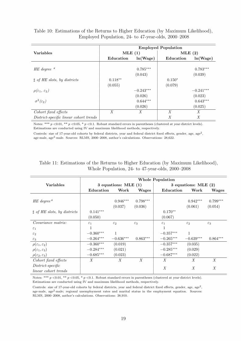
Table 10: Estimations of the Returns to Higher Education (by Maximum Likelihood),Employed Population, 24- to 47-year-olds, 2000–2008
Variables
Employed Population
MLE (1) MLE (2)
Education ln(Wage) Education ln(Wage)
HE degree * 0.785∗∗∗ 0.783∗∗∗
(0.043) (0.039)
] of HE slots, by districts 0.118∗∗ 0.150∗
(0.055) (0.079)
ρ(ε1, ε2) −0.243∗∗∗ −0.241∗∗∗
(0.026) (0.023)
σ2(ε2) 0.644∗∗∗ 0.643∗∗∗
(0.026) (0.025)
Cohort fixed effects X X X X
District-specific linear cohort trends X X
Notes: *** p <0.01, ** p <0.05, * p <0.1. Robust standard errors in parentheses (clustered at year·district levels).
Estimations are conducted using IV and maximum likelihood methods, respectively.
Controls: size of 17-year-old cohorts by federal districts, year and federal district fixed effects, gender, age, age2,
age·male, age2·male. Sources: RLMS, 2000–2008, author’s calculations. Observations: 28,622.
Table 11: Estimations of the Returns to Higher Education (by Maximum Likelihood),Whole Population, 24- to 47-year-olds, 2000–2008
Variables
Whole Population
3 equations: MLE (1) 3 equations: MLE (2)
Education Work Wages Education Work Wages
HE degree* 0.946∗∗∗ 0.798∗∗∗ 0.942∗∗∗ 0.799∗∗∗
(0.037) (0.036) (0.061) (0.054)
] of HE slots, by districts 0.141∗∗∗ 0.170∗∗
(0.050) (0.067)
Covariance matrix: ε1 ε2 ε3 ε1 ε2 ε3ε1 1 1
ε2 −0.360∗∗∗ 1 −0.357∗∗∗ 1
ε3 −0.264∗∗∗ −0.636∗∗∗ 0.863∗∗∗ −0.265∗∗∗ −0.639∗∗∗ 0.864∗∗∗
ρ(ε1, ε2) −0.360∗∗∗ (0.019) −0.357∗∗∗ (0.035)
ρ(ε1, ε3) −0.284∗∗∗ (0.021) −0.285∗∗∗ (0.029)
ρ(ε2, ε3) −0.685∗∗∗ (0.023) −0.687∗∗∗ (0.022)
Cohort fixed effects X X X X X X
District-specificX X X
linear cohort trends
Notes: *** p <0.01, ** p <0.05, * p <0.1. Robust standard errors in parentheses (clustered at year·district levels).
Estimations are conducted using IV and maximum likelihood methods, respectively.
Controls: size of 17-year-old cohorts by federal districts, year and federal district fixed effects, gender, age, age2,
age·male, age2·male; regional unemployment rates and marital status in the employment equation. Sources:
RLMS, 2000–2008, author’s calculations. Observations: 38,910.
19
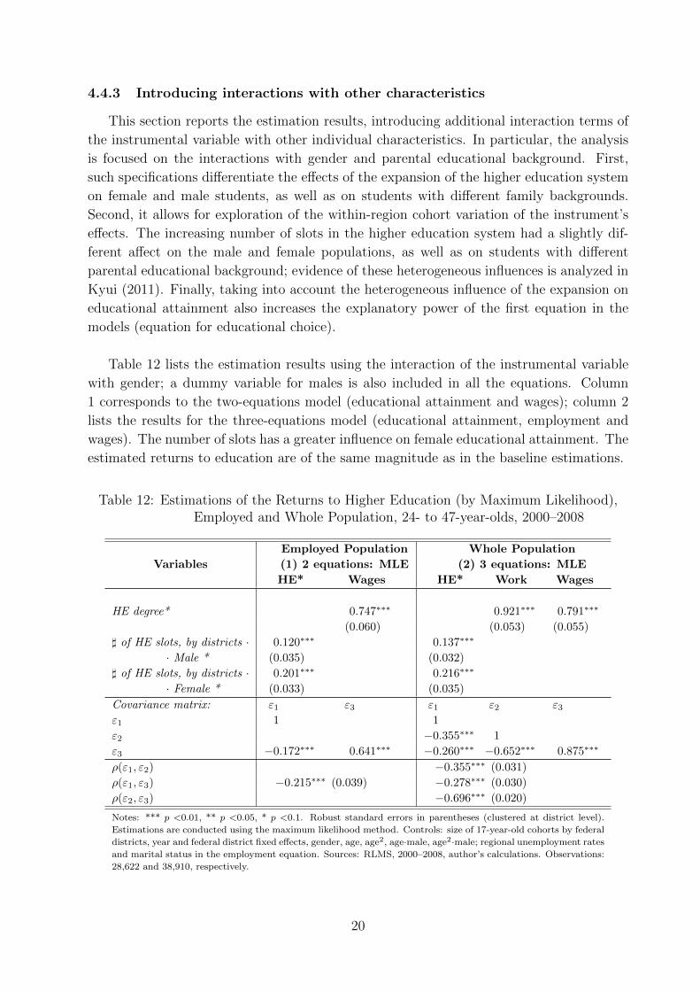
4.4.3 Introducing interactions with other characteristics
This section reports the estimation results, introducing additional interaction terms of
the instrumental variable with other individual characteristics. In particular, the analysis
is focused on the interactions with gender and parental educational background. First,
such specifications differentiate the effects of the expansion of the higher education system
on female and male students, as well as on students with different family backgrounds.
Second, it allows for exploration of the within-region cohort variation of the instrument’s
effects. The increasing number of slots in the higher education system had a slightly dif-
ferent affect on the male and female populations, as well as on students with different
parental educational background; evidence of these heterogeneous influences is analyzed in
Kyui (2011). Finally, taking into account the heterogeneous influence of the expansion on
educational attainment also increases the explanatory power of the first equation in the
models (equation for educational choice).
Table 12 lists the estimation results using the interaction of the instrumental variable
with gender; a dummy variable for males is also included in all the equations. Column
1 corresponds to the two-equations model (educational attainment and wages); column 2
lists the results for the three-equations model (educational attainment, employment and
wages). The number of slots has a greater influence on female educational attainment. The
estimated returns to education are of the same magnitude as in the baseline estimations.
Table 12: Estimations of the Returns to Higher Education (by Maximum Likelihood),Employed and Whole Population, 24- to 47-year-olds, 2000–2008
Variables
Employed Population Whole Population
(1) 2 equations: MLE (2) 3 equations: MLE
HE* Wages HE* Work Wages
HE degree* 0.747∗∗∗ 0.921∗∗∗ 0.791∗∗∗
(0.060) (0.053) (0.055)
] of HE slots, by districts · 0.120∗∗∗ 0.137∗∗∗
· Male * (0.035) (0.032)
] of HE slots, by districts · 0.201∗∗∗ 0.216∗∗∗
· Female * (0.033) (0.035)
Covariance matrix: ε1 ε3 ε1 ε2 ε3ε1 1 1
ε2 −0.355∗∗∗ 1
ε3 −0.172∗∗∗ 0.641∗∗∗ −0.260∗∗∗ −0.652∗∗∗ 0.875∗∗∗
ρ(ε1, ε2) −0.355∗∗∗ (0.031)
ρ(ε1, ε3) −0.215∗∗∗ (0.039) −0.278∗∗∗ (0.030)
ρ(ε2, ε3) −0.696∗∗∗ (0.020)
Notes: *** p <0.01, ** p <0.05, * p <0.1. Robust standard errors in parentheses (clustered at district level).
Estimations are conducted using the maximum likelihood method. Controls: size of 17-year-old cohorts by federal
districts, year and federal district fixed effects, gender, age, age2, age·male, age2·male; regional unemployment rates
and marital status in the employment equation. Sources: RLMS, 2000–2008, author’s calculations. Observations:
28,622 and 38,910, respectively.
20
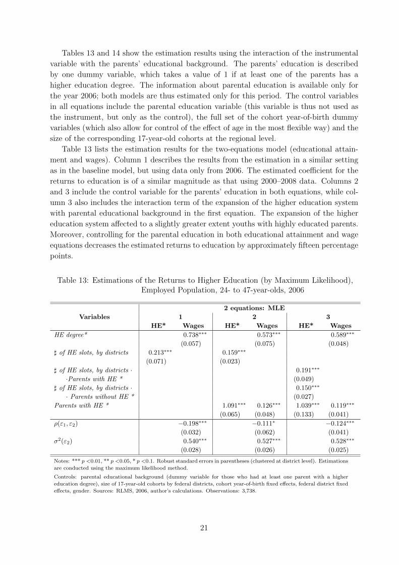
Tables 13 and 14 show the estimation results using the interaction of the instrumental
variable with the parents’ educational background. The parents’ education is described
by one dummy variable, which takes a value of 1 if at least one of the parents has a
higher education degree. The information about parental education is available only for
the year 2006; both models are thus estimated only for this period. The control variables
in all equations include the parental education variable (this variable is thus not used as
the instrument, but only as the control), the full set of the cohort year-of-birth dummy
variables (which also allow for control of the effect of age in the most flexible way) and the
size of the corresponding 17-year-old cohorts at the regional level.
Table 13 lists the estimation results for the two-equations model (educational attain-
ment and wages). Column 1 describes the results from the estimation in a similar setting
as in the baseline model, but using data only from 2006. The estimated coefficient for the
returns to education is of a similar magnitude as that using 2000–2008 data. Columns 2
and 3 include the control variable for the parents’ education in both equations, while col-
umn 3 also includes the interaction term of the expansion of the higher education system
with parental educational background in the first equation. The expansion of the higher
education system affected to a slightly greater extent youths with highly educated parents.
Moreover, controlling for the parental education in both educational attainment and wage
equations decreases the estimated returns to education by approximately fifteen percentage
points.
Table 13: Estimations of the Returns to Higher Education (by Maximum Likelihood),Employed Population, 24- to 47-year-olds, 2006
Variables
2 equations: MLE
1 2 3
HE* Wages HE* Wages HE* Wages
HE degree* 0.738∗∗∗ 0.573∗∗∗ 0.589∗∗∗
(0.057) (0.075) (0.048)
] of HE slots, by districts 0.213∗∗∗ 0.159∗∗∗
(0.071) (0.023)
] of HE slots, by districts · 0.191∗∗∗
·Parents with HE * (0.049)
] of HE slots, by districts · 0.150∗∗∗
· Parents without HE * (0.027)
Parents with HE * 1.091∗∗∗ 0.126∗∗∗ 1.039∗∗∗ 0.119∗∗∗
(0.065) (0.048) (0.133) (0.041)
ρ(ε1, ε2) −0.198∗∗∗ −0.111∗ −0.124∗∗∗
(0.032) (0.062) (0.041)
σ2(ε2) 0.540∗∗∗ 0.527∗∗∗ 0.528∗∗∗
(0.028) (0.026) (0.025)
Notes: *** p <0.01, ** p <0.05, * p <0.1. Robust standard errors in parentheses (clustered at district level). Estimations
are conducted using the maximum likelihood method.
Controls: parental educational background (dummy variable for those who had at least one parent with a higher
education degree), size of 17-year-old cohorts by federal districts, cohort year-of-birth fixed effects, federal district fixed
effects, gender. Sources: RLMS, 2006, author’s calculations. Observations: 3,738.
21
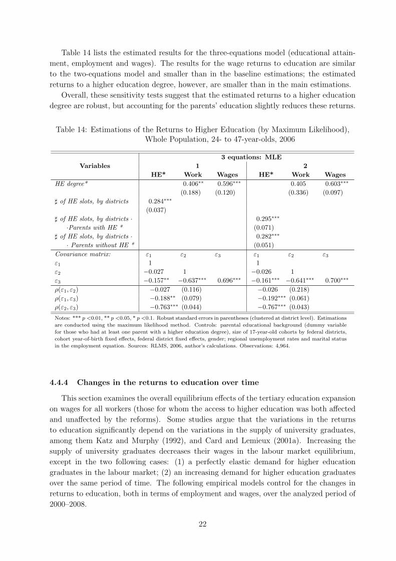
Table 14 lists the estimated results for the three-equations model (educational attain-
ment, employment and wages). The results for the wage returns to education are similar
to the two-equations model and smaller than in the baseline estimations; the estimated
returns to a higher education degree, however, are smaller than in the main estimations.
Overall, these sensitivity tests suggest that the estimated returns to a higher education
degree are robust, but accounting for the parents’ education slightly reduces these returns.
Table 14: Estimations of the Returns to Higher Education (by Maximum Likelihood),Whole Population, 24- to 47-year-olds, 2006
Variables
3 equations: MLE
1 2
HE* Work Wages HE* Work Wages
HE degree* 0.406∗∗ 0.596∗∗∗ 0.405 0.603∗∗∗
(0.188) (0.120) (0.336) (0.097)
] of HE slots, by districts 0.284∗∗∗
(0.037)
] of HE slots, by districts · 0.295∗∗∗
·Parents with HE * (0.071)
] of HE slots, by districts · 0.282∗∗∗
· Parents without HE * (0.051)
Covariance matrix: ε1 ε2 ε3 ε1 ε2 ε3ε1 1 1
ε2 −0.027 1 −0.026 1
ε3 −0.157∗∗ −0.637∗∗∗ 0.696∗∗∗ −0.161∗∗∗ −0.641∗∗∗ 0.700∗∗∗
ρ(ε1, ε2) −0.027 (0.116) −0.026 (0.218)
ρ(ε1, ε3) −0.188∗∗ (0.079) −0.192∗∗∗ (0.061)
ρ(ε2, ε3) −0.763∗∗∗ (0.044) −0.767∗∗∗ (0.043)
Notes: *** p <0.01, ** p <0.05, * p <0.1. Robust standard errors in parentheses (clustered at district level). Estimations
are conducted using the maximum likelihood method. Controls: parental educational background (dummy variable
for those who had at least one parent with a higher education degree), size of 17-year-old cohorts by federal districts,
cohort year-of-birth fixed effects, federal district fixed effects, gender; regional unemployment rates and marital status
in the employment equation. Sources: RLMS, 2006, author’s calculations. Observations: 4,964.
4.4.4 Changes in the returns to education over time
This section examines the overall equilibrium effects of the tertiary education expansion
on wages for all workers (those for whom the access to higher education was both affected
and unaffected by the reforms). Some studies argue that the variations in the returns
to education significantly depend on the variations in the supply of university graduates,
among them Katz and Murphy (1992), and Card and Lemieux (2001a). Increasing the
supply of university graduates decreases their wages in the labour market equilibrium,
except in the two following cases: (1) a perfectly elastic demand for higher education
graduates in the labour market; (2) an increasing demand for higher education graduates
over the same period of time. The following empirical models control for the changes in
returns to education, both in terms of employment and wages, over the analyzed period of
2000–2008.
22
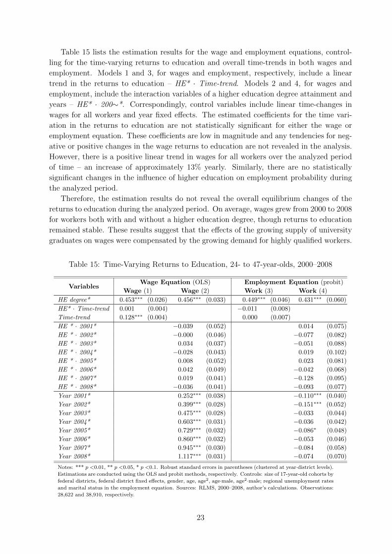
Table 15 lists the estimation results for the wage and employment equations, control-
ling for the time-varying returns to education and overall time-trends in both wages and
employment. Models 1 and 3, for wages and employment, respectively, include a linear
trend in the returns to education – HE* · Time-trend. Models 2 and 4, for wages and
employment, include the interaction variables of a higher education degree attainment and
years – HE* · 200∼*. Correspondingly, control variables include linear time-changes in
wages for all workers and year fixed effects. The estimated coefficients for the time vari-
ation in the returns to education are not statistically significant for either the wage or
employment equation. These coefficients are low in magnitude and any tendencies for neg-
ative or positive changes in the wage returns to education are not revealed in the analysis.
However, there is a positive linear trend in wages for all workers over the analyzed period
of time – an increase of approximately 13% yearly. Similarly, there are no statistically
significant changes in the influence of higher education on employment probability during
the analyzed period.
Therefore, the estimation results do not reveal the overall equilibrium changes of the
returns to education during the analyzed period. On average, wages grew from 2000 to 2008
for workers both with and without a higher education degree, though returns to education
remained stable. These results suggest that the effects of the growing supply of university
graduates on wages were compensated by the growing demand for highly qualified workers.
Table 15: Time-Varying Returns to Education, 24- to 47-year-olds, 2000–2008
VariablesWage Equation (OLS) Employment Equation (probit)
Wage (1) Wage (2) Work (3) Work (4)
HE degree* 0.453∗∗∗ (0.026) 0.456∗∗∗ (0.033) 0.449∗∗∗ (0.046) 0.431∗∗∗ (0.060)
HE* · Time-trend 0.001 (0.004) −0.011 (0.008)
Time-trend 0.128∗∗∗ (0.004) 0.000 (0.007)
HE * · 2001* −0.039 (0.052) 0.014 (0.075)
HE * · 2002* −0.000 (0.046) −0.077 (0.082)
HE * · 2003* 0.034 (0.037) −0.051 (0.088)
HE * · 2004* −0.028 (0.043) 0.019 (0.102)
HE * · 2005* 0.008 (0.052) 0.023 (0.081)
HE * · 2006* 0.042 (0.049) −0.042 (0.068)
HE * · 2007* 0.019 (0.041) −0.128 (0.095)
HE * · 2008* −0.036 (0.041) −0.093 (0.077)
Year 2001* 0.252∗∗∗ (0.038) −0.110∗∗∗ (0.040)
Year 2002* 0.399∗∗∗ (0.028) −0.151∗∗∗ (0.052)
Year 2003* 0.475∗∗∗ (0.028) −0.033 (0.044)
Year 2004* 0.603∗∗∗ (0.031) −0.036 (0.042)
Year 2005* 0.729∗∗∗ (0.032) −0.086∗ (0.048)
Year 2006* 0.860∗∗∗ (0.032) −0.053 (0.046)
Year 2007* 0.945∗∗∗ (0.030) −0.084 (0.058)
Year 2008* 1.117∗∗∗ (0.031) −0.074 (0.070)
Notes: *** p <0.01, ** p <0.05, * p <0.1. Robust standard errors in parentheses (clustered at year·district levels).
Estimations are conducted using the OLS and probit methods, respectively. Controls: size of 17-year-old cohorts by
federal districts, federal district fixed effects, gender, age, age2, age·male, age2·male; regional unemployment rates
and marital status in the employment equation. Sources: RLMS, 2000–2008, author’s calculations. Observations:
28,622 and 38,910, respectively.
23
5 Heterogeneous Returns to Higher Education
This section explores the heterogeneity in the returns to higher education, by allowing
them to vary with both observable and unobservable individual characteristics that affect
the decision to pursue higher education. This is done by estimating the marginal returns
to education and using the model with essential heterogeneity.
The previous sections refer to the framework of instrumental variables. IV provides an
estimation of the local average treatment effect – the returns to higher education for those
who switched to higher education because of the changes in the instrument (in this study’s
case, the growing opportunities in access to higher education), who would not otherwise
have pursued higher education. However, the local average treatment effect does not nec-
essarily correspond to the average treatment effect in the population, in other words, to the
average returns to education in the population (the average treatment effect is usually the
main parameter of interest in the treatment evaluation). Thus, Heckman (1997), Heckman
et al. (2003), and Carneiro et al. (2001) show that, in the presence of heterogeneity in
the returns to education and selection on the gains (namely, students taking into account
their heterogeneous returns while choosing their educational attainment), OLS and IV are
not consistent estimators of the mean returns to education in the population. It is pos-
sible to identify, under certain assumptions, the heterogeneous returns to education with
the marginal treatment effects (MTE) estimation via the method of local instrumental
variables (LIV). The MTE for the returns to education estimation is the average return
to schooling for individuals who are indifferent to accessing education at varying levels
of unobservable characteristics, which influence this educational choice along with other
observable characteristics that can be accounted for. The concept of MTE was first intro-
duced by Bjorklund and Moffitt (1987). Carneiro et al. (2001), Heckman et al. (2006), and
Heckman and Vytlacil (2007) develop the theoretical framework of MTE estimation for
the returns to schooling; derive the identification of the average treatment effect (ATE),
treatment on the treated (TT), and treatment on the untreated (TUT); and also provide
the empirical applications of these methods for U.S. data. Heckman and Li (2003) and
Wang et al. (2007) apply these methods to the estimation of the returns to education in
China.
5.1 Returns to education: model with essential heterogeneity
The educational choice, obtaining a higher education degree, is expressed by the variable
Si, which takes a value of 1 for those with high education, and 0 otherwise. The returns
to education θi vary in the population:
lnWi = α + β ·Xi + θi · Si + Ui. (1)
In the literature, such a model is referred to as “random coefficient” or “heterogeneous
treatment effect” models (Heckman et al. (2006)). There are two potential wage outcomes
(for workers with and without higher education):
24
{lnW1,i = α1 + β1 ·Xi + U1,i, if Si = 1,
lnW0,i = α0 + β0 ·Xi + U0,i, if Si = 0.(2)
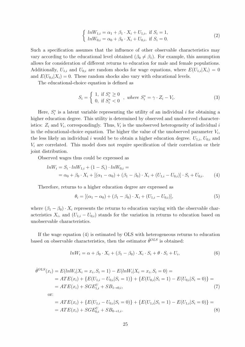
Such a specification assumes that the influence of other observable characteristics may
vary according to the educational level obtained (β0 6= β1). For example, this assumption
allows for consideration of different returns to education for male and female populations.
Additionally, U1,i and U0,i are random shocks for wage equations, where E(U1,i|Xi) = 0
and E(U0,i|Xi) = 0. These random shocks also vary with educational levels.
The educational-choice equation is defined as
Si =
{1, if S∗i ≥ 0
0, if S∗i < 0, where S∗i = γ · Zi − Vi. (3)
Here, S∗i is a latent variable representing the utility of an individual i for obtaining a
higher education degree. This utility is determined by observed and unobserved character-
istics: Zi and Vi, correspondingly. Thus, Vi is the unobserved heterogeneity of individual i
in the educational-choice equation. The higher the value of the unobserved parameter Vi,
the less likely an individual i would be to obtain a higher education degree. U1,i, U0,i and
Vi are correlated. This model does not require specification of their correlation or their
joint distribution.
Observed wages thus could be expressed as
lnWi = Si · lnW1,i + (1− Si) · lnW0,i =
= α0 + β0 ·Xi + [(α1 − α0) + (β1 − β0) ·Xi + (U1,i − U0,i)] · Si + U0,i. (4)
Therefore, returns to a higher education degree are expressed as
θi = [(α1 − α0) + (β1 − β0) ·Xi + (U1,i − U0,i)], (5)
where (β1 − β0) ·Xi represents the returns to education varying with the observable char-
acteristics Xi, and (U1,i − U0,i) stands for the variation in returns to education based on
unobservable characteristics.
If the wage equation (4) is estimated by OLS with heterogeneous returns to education
based on observable characteristics, then the estimator θ̂OLS is obtained:
lnWi = α + β0 ·Xi + (β1 − β0) ·Xi · Si + θ · Si + Ui, (6)
θ̂OLS(xi) = E(lnWi|Xi = xi, Si = 1)− E(lnWi|Xi = xi, Si = 0) =
= ATE(xi) + {E(U1,i − U0,i|Si = 1)}+ {E(U0,i|Si = 1)− E(U0,i|Si = 0)} =
= ATE(xi) + SGEU1,i + SB1→0,i, (7)
or:
= ATE(xi) + {E(U1,i − U0,i|Si = 0)}+ {E(U1,i|Si = 1)− E(U1,i|Si = 0)} =
= ATE(xi) + SGEU0,i + SB0→1,i. (8)
25
Therefore, the bias of the OLS estimator in estimating the ATE can be decomposed
into two components: sorting on the gains effect (SGE) and selection bias (SB).
The selection bias SB1→0,i = E(U0,i|Si = 1) − E(U0,i|Si = 0) describes the fact that
unobservable factors, which influence the decision to obtain a higher education degree,
affect wages. It shows the difference in wages between those who obtain higher education
and those who do not in the case where neither of the two would have earned a higher
education degree.
Sorting on the gains effect SGEU1,i = E(U1,i − U0,i|Si = 1) represents the mean gain in
unobservable components of the wage equation for people who choose a higher education
degree Si = 1. The non-zero value of the sorting on the gains effect means that individuals
self-select for higher education based on their wage returns to unobservable characteristics
in the case of either obtaining, or not obtaining, a higher education degree. The positive
sign for the SGEU1,i means that individuals with a degree have unobservable characteristics,
which will be better paid if they obtain this level of education.
Similarly, sorting on the gains effect causes a bias in the IV estimation of the ATE
(using Ii as the instrument, which is correlated to the Vi but is not correlated to the Ui,
U1,i, U0,i):
θ̂IV (xi) =Cov(Ii, lnWi)
Cov(Ii, Si)= (9)
= ATE(xi) +Cov(Ii, (U1,i − U0,i)|Si = 1) · Pr(Si = 1|xi, Ii)
Cov(Ii, Si).
Consequently, the IV estimator would be equal to the ATE (thus LATE = ATE) only
if either (1) U1,i − U0,i = 0, indicating no heterogeneity in the returns to education, or (2)
U1,i − U0,i is independent of Si, meaning no sorting on gains. In the absence of essential
heterogeneity (i.e., in cases of people not sorting themselves based on the gains on unob-
servables), the IV is a consistent estimator of the ATE. However, in the presence of sorting
on the gains, IV may overestimate the ATE by putting more weight on the returns for
treated individuals (Heckman (1997)).
In the frame of the model with essential heterogeneity, the effects of treatment on the
treated (TT) and the effects of treatment on the untreated (TUT) can be written as follows:
TT (xi) = E(lnW1,i − lnW0,i|Xi = xi, Si = 1) = ATE(xi) + SGEU1,i, (10)
TUT (xi) = E(lnW1,i − lnW0,i|Xi = xi, Si = 0) = ATE(xi) + SGEU0,i, (11)
where SGEU1,i is the sorting on the gains effect for those who obtain a higher education
degree, and SGEU0,i represents the sorting on the gains effect for those who do not (the
latter representing their returns to unobservable characteristics if they would have obtained
a degree).
26
The average effects in the population, therefore, could be written as16:
ATE =
∫X
ATE(xi) dFX(x); TT =
∫X|S=1
TT (xi) dFX|S=1(x), (13)
TUT =
∫X|S=0
TUT (xi) dFX|S=0(x); θ̂OLS = ATE + SGE1 + SB1→0.
The MTE estimation is used in order to calculate all these parameters properly:
MTE(Xi = x, US,i = us = p) = E(lnW1,i − lnW0,i|Xi = x, US,i = us) =
=∂E(lnWi|Xi = x, P (Zi) = p)
∂p
∣∣∣∣∣p=us
, (14)
where, US,i is the uniform transformation of the random term of the educational equation
Vi: US = FV (V ), US Unif [0, 1]. Therefore, the educational-choice equation (3) can be
rewritten as follows:
Si =
{1, if γ · Zi − Vi ≥ 0
0, if γ · Zi − Vi < 0=
{1, if FV (γ · Zi) ≥ FV (Vi)
0, if FV (γ · Zi) < FV (Vi)=
=
{1, if P (Zi) ≥ US,i0, if P (Zi) < US,i
. (15)
The MTE measures the returns to education (average treatment effect) at the points
us of marginal changes in US (in other words, at the points of marginal changes of V , the
unobservable component in the educational-choice equation). Since these are measured
at the points of P (Zi) = p = us, at these values of the unobservable component in the
educational-choice equation, individuals are indifferent about seeking a higher education
degree. Therefore, the MTE is the marginal willingness to pay for the lnW1,i versus lnW0,i,
given the observed characteristics Xi and the level of unobserved characteristics US,i = us.
The small values of us (close to 0) mean that the small values of V (large values of −V ) are
therefore associated with people who are more likely to obtain a higher education degree,
given their unobservable characteristics. Correspondingly, MTE measured for large values
of us (close to 1) shows the returns to education for people less likely to obtain higher
education, based on their unobservable characteristics.
Heckman and Vytlacil (1999), Heckman et al. (2006), and Heckman and Vytlacil (2007)
show that ATE, TT and TUT could be determined as the weighted averages of MTE, ac-
cording to the formulas (25), described in section 3 of the Technical Appendix. The weights
16Note that in considering the population effects, the effect of the sorting on gains can be based on theobservable characteristics if E(X|S = 1) 6= E(X|S = 0) 6= E(X), in other words, if people sort themselvesbased on the observable characteristics. For example, if female workers have higher returns to education,they may seek higher education more often than male workers. Therefore, the sorting on the gains effectsfor the population is written as
TT = ATE + SGEU1 + (β1 − β0) · (E(X|S = 1)− E(X)),
TUT = ATE + SGEU0 + (β1 − β0) · (E(X|S = 0)− E(X)). (12)
27
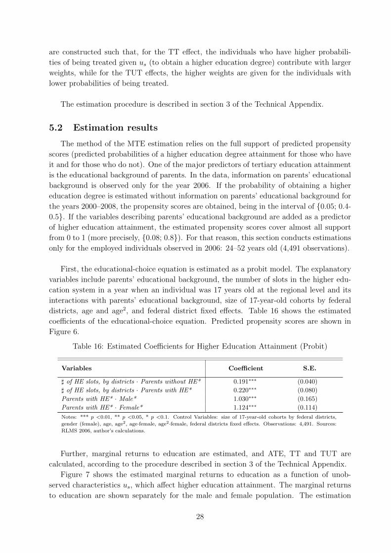
are constructed such that, for the TT effect, the individuals who have higher probabili-
ties of being treated given us (to obtain a higher education degree) contribute with larger
weights, while for the TUT effects, the higher weights are given for the individuals with
lower probabilities of being treated.
The estimation procedure is described in section 3 of the Technical Appendix.
5.2 Estimation results
The method of the MTE estimation relies on the full support of predicted propensity
scores (predicted probabilities of a higher education degree attainment for those who have
it and for those who do not). One of the major predictors of tertiary education attainment
is the educational background of parents. In the data, information on parents’ educational
background is observed only for the year 2006. If the probability of obtaining a higher
education degree is estimated without information on parents’ educational background for
the years 2000–2008, the propensity scores are obtained, being in the interval of {0.05; 0.4-
0.5}. If the variables describing parents’ educational background are added as a predictor
of higher education attainment, the estimated propensity scores cover almost all support
from 0 to 1 (more precisely, {0.08; 0.8}). For that reason, this section conducts estimations
only for the employed individuals observed in 2006: 24–52 years old (4,491 observations).
First, the educational-choice equation is estimated as a probit model. The explanatory
variables include parents’ educational background, the number of slots in the higher edu-
cation system in a year when an individual was 17 years old at the regional level and its
interactions with parents’ educational background, size of 17-year-old cohorts by federal
districts, age and age2, and federal district fixed effects. Table 16 shows the estimated
coefficients of the educational-choice equation. Predicted propensity scores are shown in
Figure 6.
Table 16: Estimated Coefficients for Higher Education Attainment (Probit)
Variables Coefficient S.E.
] of HE slots, by districts · Parents without HE* 0.191∗∗∗ (0.040)
] of HE slots, by districts · Parents with HE* 0.220∗∗∗ (0.080)
Parents with HE* · Male* 1.030∗∗∗ (0.165)
Parents with HE* · Female* 1.124∗∗∗ (0.114)
Notes: *** p <0.01, ** p <0.05, * p <0.1. Control Variables: size of 17-year-old cohorts by federal districts,
gender (female), age, age2, age·female, age2·female, federal districts fixed effects. Observations: 4,491. Sources:
RLMS 2006, author’s calculations.
Further, marginal returns to education are estimated, and ATE, TT and TUT are
calculated, according to the procedure described in section 3 of the Technical Appendix.
Figure 7 shows the estimated marginal returns to education as a function of unob-
served characteristics us, which affect higher education attainment. The marginal returns
to education are shown separately for the male and female population. The estimation
28
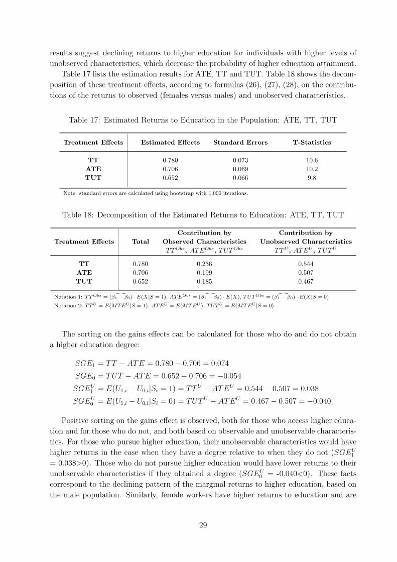
results suggest declining returns to higher education for individuals with higher levels of
unobserved characteristics, which decrease the probability of higher education attainment.
Table 17 lists the estimation results for ATE, TT and TUT. Table 18 shows the decom-
position of these treatment effects, according to formulas (26), (27), (28), on the contribu-
tions of the returns to observed (females versus males) and unobserved characteristics.
Table 17: Estimated Returns to Education in the Population: ATE, TT, TUT
Treatment Effects Estimated Effects Standard Errors T-Statistics
TT 0.780 0.073 10.6
ATE 0.706 0.069 10.2
TUT 0.652 0.066 9.8
Note: standard errors are calculated using bootstrap with 1,000 iterations.
Table 18: Decomposition of the Estimated Returns to Education: ATE, TT, TUT
Treatment Effects Total
Contribution by Contribution by
Observed Characteristics Unobserved Characteristics
TTObs, ATEObs, TUTObs TTU , ATEU , TUTU
TT 0.780 0.236 0.544
ATE 0.706 0.199 0.507
TUT 0.652 0.185 0.467
Notation 1: TTObs = ( ̂β1 − β0) · E(X|S = 1), ATEObs = ( ̂β1 − β0) · E(X), TUTObs = ( ̂β1 − β0) · E(X|S = 0)
Notation 2: TTU = E(MTEU |S = 1), ATEU = E(MTEU ), TUTU = E(MTEU |S = 0)
The sorting on the gains effects can be calculated for those who do and do not obtain
a higher education degree:
SGE1 = TT − ATE = 0.780− 0.706 = 0.074
SGE0 = TUT − ATE = 0.652− 0.706 = −0.054
SGEU1 = E(U1,i − U0,i|Si = 1) = TTU − ATEU = 0.544− 0.507 = 0.038
SGEU0 = E(U1,i − U0,i|Si = 0) = TUTU − ATEU = 0.467− 0.507 = −0.040.
Positive sorting on the gains effect is observed, both for those who access higher educa-
tion and for those who do not, and both based on observable and unobservable characteris-
tics. For those who pursue higher education, their unobservable characteristics would have
higher returns in the case when they have a degree relative to when they do not (SGEU1
= 0.038>0). Those who do not pursue higher education would have lower returns to their
unobservable characteristics if they obtained a degree (SGEU0 = -0.040<0). These facts
correspond to the declining pattern of the marginal returns to higher education, based on
the male population. Similarly, female workers have higher returns to education and are
29

more likely to attain a higher education degree (SGE1 - SGEU1 = 0.074-0.038 = 0.036>0).
This sorting on the gains determines the differences between the TT, ATE and TUT effects.
Selection effects take the following value:
SB1→0,i = E(U0,i|Si = 1)− E(U0,i|Si = 0) = θ̂OLS − TTU = 0.327− 0.544 = −0.217
SB0→1,i = E(U1,i|Si = 1)− E(U1,i|Si = 0) = θ̂OLS − TUTU = 0.327− 0.467 = −0.140.
A negative selection effect can be observed for those who pursue higher education.
Those who have a higher education degree would have lower wage returns to their unob-
servable characteristics if they did not have a higher education degree, in comparison to
those who do not currently have a degree. If education was provided to everybody, the
difference in wages between those who attain it now and those who do not would be lower
in absolute value than if higher education were forbidden for all (0.140 versus 0.217).
Overall, the estimated average returns to education in the population are similar to
that obtained by IV, thus similar to the local average treatment effect of attainment of a
higher education degree. This fact is due to the low magnitude of the sorting on the gains
effect, which constitutes the bias of the IV estimator for the average returns to education,
or in other words, which accounts for the difference between the local average treatment
effect and the average treatment effect of a higher education degree. Returns to a higher
education degree decrease with the unobservable characteristics, which reduce the proba-
bility of obtaining higher education (as shown by the estimation of the marginal returns
to education). Those who increase their educational attainment alongside the increasing
access to higher education likely have higher values of unobservable characteristics, which
decrease the probability of higher education attainment, than those who attain it when
access to higher education is tighter. Those who increasingly pursue higher education when
access to higher education becomes greater would thus have lower returns to education.
This observed pattern of declining returns to higher education in the population could
have several explanations. First, within the theoretical framework of education “enhancing
productivity,” the returns to higher education could be lower for people with lower abil-
ity levels. Expansion of the higher education system in Russia provided an opportunity to
increase educational attainment for a portion of the population. Since selection to universi-
ties was competitive, based on individual abilities, the periods with greater access to higher
education are thus characterized by a lower average level of ability of university entrants.
Second, within the framework of the “signalling” theory, when education is considered as
a “signal of ability,” the labour market would reward higher education with a lower payoff
when the signal of ability is less precise. When a larger cohort of higher education gradu-
ates comes to the labour market, the signal of ability is more vague compared with that of
periods of stricter access to higher education. Thus, the expansion of the higher education
system makes people both with and without higher education degrees worse in terms of
the average level of ability. Therefore, the signal of ability through educational attainment
becomes more fuzzy, and the labour market could lower the returns to higher education
30

for that reason. Finally, the expansion of higher education could have occurred to a differ-
ent extent for high-quality and low-quality universities, as well as within different majors.
Such a changing composition within the educational system could impact the returns to
education.17 However, the current study analyzes neither the changes in the average qual-
ity of educational institutions and the resulting influence on the returns to education, nor
the changing composition of majors among graduates. Instead, this study focuses on the
average returns to a higher education degree, averaged by major and university quality.
Nevertheless, analysis of the effects of changing educational quality and the composition
of major could be a promising direction for further research.
6 Conclusion
This paper analyzes the effects of a 15-year expansion of the Russian Federation edu-
cational system on labour market outcomes. It identifies the returns to education for the
population and quantifies the effects of this expansion on employment and wages.
The study reports evidence of significant returns to higher education in terms of both
employment and wages. However, these returns are slightly smaller when controlling for
parents’ educational background. No significant equilibrium effects of this expansion on
wages are revealed. The estimation results of the marginal returns to education suggest
declining returns to education in the population, based on unobservable characteristics
negatively affecting higher education attainment. This study determines a light positive
sorting on the gains, meaning that youths self-select to universities based on their expected
returns to education. However, this sorting is low in magnitude, and thus similar estimation
results are obtained for the returns to education using the IV and MTE methods.
Expansion of the higher education system in Russia during 1990–2005 therefore had
positive effects on wages for those who increased their educational attainment. However,
their returns to education were lower than those of youths who obtained a higher education
degree during the periods of tougher access to universities.
The large expansion of the higher education system in Russia provides an exogenous
variation in access to higher education, significantly increasing university enrolment. This
study estimates the effects of such expansion specifically on labour market outcomes. How-
ever, this natural experiment could potentially be used to analyze the influence of educa-
tion on other life outcomes: occupational choices, work-life balance, marriages (including a
partner’s “quality”), childbearing decisions (number and timing of births, time dedicated
to children’s education), educational outcomes of children of the next generation, health
attitudes, risky behaviour, etc. These questions are potential topics for future research,
for which the transition reforms in the Russian Federation could serve as an identification
strategy for the parameters determining the importance of education.
17For instance, characteristics such as the student-teacher ratio and student-educational surface sizeratio could serve as proxies for quality of higher education (being negatively correlated with it). Lookingat these ratios over the analyzed period, there was a small increase in these measures in the beginning ofexpansion followed by a stabilization and decrease. Moreover, the increasing proportion of social sciencemajors (such as economics and law) is also observed during this period.
31

References
Angrist, J.D., G.W. Imbens, and D.B. Rubin. 1996. “Identification of Causal Effects Using InstrumentalVariables.” Journal of the American Statistical Association 91(434): 444–455.
Angrist, J.D. and A.B. Krueger. 1991. “Does Compulsory School Attendance Affect Schooling and Earn-ings?” Quarterly Journal of Economics 106(4): 979–1014.
Angrist, J.D. and J.S. Pischke. 2009. “Mostly Harmless Econometrics: An Empiricist’s Companion.”Princeton University Press .
Arcidiacono, P. 2005. “Affirmative Action in Higher Education: How Do Admission and Financial AidRules Affect Future Earnings?” Econometrica 73(5 (Sept.)): 1477–1524.
Belokonnaya, L., V. Gimpelson, T. Gorbacheva, O. Gihareva, R. Kapelushnikov, and A. Lukianova. 2007.“Wage formation: analysis in the light of work professions.” Wages in the Russian Federation: Evolutionand Differentiation. Moscow: State University Higher School of Economics.
Belzil, C. 2006. “The Return to Schooling in Structural Dynamic Models: A Survey.” IZA DiscussionPaper No. 2370.
Bjorklund, A. and R. Moffitt. 1987. “The Estimation of Wage Gains and Welfare Gains in Self-SelectionModels.” Review of Economics and Statistics 69.
Card, D. 1995. “Using Geographic Variation in College Proximity to Estimate the Return to Schooling.”Aspects of Labour Market Behaviour: Essays in Honour of John Vanderkamp, by L.N. Christofides,E.K. Grant, R. Swidinsky 201–222.
———. 1999. “The Causal Effect of Education on Earnings.” Handbook of Labor Economics 3: 1801–1863.
Card, D. and T. Lemieux. 2001a. “Can Falling Supply Explain the Rising Return to College for YoungMen.” Quarterly Journal of Economics 116: 705–746.
———. 2001b. “Education, Earnings, and the “Canadian G.I. Bill”.” Canadian Journal of Economics34(2): 313–344.
Carneiro, P., J. Heckman, and E. Vytlacil. 2001. “Estimating the Return to Education When It VariesAmong Individuals.” Working Paper, University of Chicago.
Cheidvasser, S. and H. Benitez-Silva. 2007. “The Educated Russian’s Curse: Returns to Education in theRussian Federation During the 1990s.” Labor 21(1): 1–41.
Conneely, K. and R. Uusitalo. 1997. “Estimating Heterogeneous Treatment Effects in the Becker SchoolingModel.” Discussion Paper, Industrial Relations Sections, Princeton University.
Duflo, E. 2001. “Consequences of School Construction in Indonesia.” The American Economic Review91(4): 795–813.
Froelich, M. and B. Melly. 2008. “Unconditional quantile treatment effects under endogeneity.” IZADiscussion Paper No. 3288.
———. 2010. “Estimation of quantile treatment effects with STATA.” Stata Journal.
Gohberg, L.M., I.U. Zabaturina, N.V. Kovaleva, V.I. Kuznetsova, O.K. Ozerova, and L.A. Rosovetskaya.2007. Education in the Russian Federation. Statistical Yearbook. SU-HSE, Moscow.
Gregory, P. and J. Kohlhase. 1988. “The Earnings of Soviet Workers: Evidence from The Soviet InterviewProject.” The Review of Economics and Statistics 70(1).
Heckman, J.J. 1997. “Instrumental Variables: A Study of Implicit Behavioral Assumptions Used in MakingProgram Evaluations.” Journal of Human Resources 32(3): 441–462.
32
Heckman, J.J. and X. Li. 2003. “Selection Bias, Comparative Advantage and Heterogeneous Returns toEducation: Evidence from China in 2000.” IFAU Working Paper No. 17.
Heckman, J.J., L.J. Lochner, and P.E. Todd. 2003. “Fifty Years of Mincer Earnings Regressions.” NBERWorking Paper No. 9732.
Heckman, J.J., S. Urzua, and E. Vytlacil. 2006. “Understanding Instrumental Variables in Models withEssential Heterogeneity.” Review of Economics and Statistics 88(3).
Heckman, J.J. and E. Vytlacil. 1999. “Local Instrumental Variable and Latent Variable Models for Iden-tifying and Bounding Treatment Effects.” Proceedings of the National Academy of Sciences, No. 96.
———. 2007. “Econometric Evaluation of Social Programs.” Handbook of Econometrics.
ISCED. 2006. “International Standard Classification of Education (ISCED) 1997.” UNESCO Institute forStatistics.
Kane, T.J. and C.E. Rouse. 1993. “Labor Market Returns to Two- and Four-Year Colleges: is a Credit aCredit and Do Degrees Matter?” NBER Working Paper No. 4268.
Katz, K. 1999. “Were there no returns to education in the USSR? Estimates from Soviet-period householddata.” Labor Economics (6).
Katz, L. and K. Murphy. 1992. “Changes in Relative Wages, 1963-1987: Supply and Demand Factors.”Quarterly Journal of Economics 107: 35–78.
Kyui, N. 2011. “Microeconometric Analysis of Tertiary Education Demand and Returns to Education.”PhD Dissertation, Paris School of Economics - University Paris-1 Pantheon Sorbonne .
Lukov, V.A. 2005. “Educational Reforms.” Encyclopaedia of the Humanities (3): 217–219.
OECD. 2013. “Education at a Glance 2013: OECD Indicators.” OECD Publishing(http://dx.doi.org/10.1787/eag-2013-en).
Ofer, G. and A. Vinokur. 1992. The Soviet Household Under the Old Regime. Economic Conditions andBehaviour in the 1970s. CUP, Cambridge.
Oreopoulos, P. 2006a. “The Compelling Effects of Compulsory Schooling: Evidence from Canada.” Cana-dian Journal of Economics 39(1): 22–52.
———. 2006b. “Estimating Average and Local Average Treatment Effects of Education when CompulsorySchooling Laws Really Matter.” The American Economic Review 96(1): 152–175.
Pischke, S. and T. von Wachter. 2008. “Zero Returns to Compulsory Schooling in Germany: Evidence andInterpretation.” Review of Economics and Statistics 90(3): 592–598.
Robinson, P. 1988. “Root-N consistent semiparametric regression.” Econometrica (56): 931–954.
Swafford, M., M. Kosolapov, and P. Kozyreva. 1999a. “International standards for evaluating surveyresearch.” Universe of Russia 1-2: 281–302.
———. 1999b. “The Russian Longitudinal Monitoring Survey: Measuring the Well-Being of Russiansduring the 1990s.” Universe of Russia 3: 153–172.
Walker, I. and Y. Zhu. 2008. “The College Wage Premium and the Expansion of Higher Education in theUK.” Scandinavian Journal of Economics 110(4): 695–709.
Wang, X., B.M. Fleisher, H. Li, and S. Li. 2007. “Access to Higher Education and Inequality: The ChineseExperiment.” IZA Working Paper No. 2823.
33

Figure 1: Number of Tertiary Education Students in Russia and OECD countriesper 1,000 inhabitants (in %)
3634
31 32
36
44
55
60
6567
15
25
35
45
55
65
Number of Students in Tertiary Education per 1000 inhabitants, in %
Russian Federation
United States
Finland
Norway
Sweden
Denmark
Ireland
Spain
United Kingdom
Belgium
Netherlands
Portugal
France
Austria
Italy
Japan
Switzerland
Source: World Bank databank (http://databank.worldbank.org/data/home.aspx).
Figure 2: Higher Education System in Russia: 1970-2008
457 483 494 502 514 519 535 548 553 569 573 578 580 590 607 621 655 652 662 655 660 658 660
78157
193244
302 334 349 358387
384 392 409 413 430 450 474
0
200
400
600
800
1000
1200
Higher education establishments (universities) : public and private
Number of private universities (higher education establishments)
Number of public universities (higher education establishments)
Total number of universities (higher education establishments)
537 587 614 635 584 553 499 502 499 532 551 565 544 564 587 588 608 623 629 614 585 569 561
6994 124
183 288382
554676 692
789 756 759 791 815 802
5566
81
112
152
198204
232 275 268 281 298 279
0
200
400
600
800
1000
1200
1400
1600
1800
Number of 1st-year admitted students in higher education: public and private universities (in thousands)
Number of 1st-year admitted students in higher education:private universities, full-tuition basis
Number of 1st-year admitted students in higher education:public universities, full-tuition basis
Number of 1st-year admitted students in higher education:public universities, state-subsidized basis
Sources: Gohberg et al. (2007), Russian Federal Committee for Statistics (http://www.gks.ru)
34

Figure 3: Vocational Tertiary Education System in Russia: 1970-2008
2423 2483 2505 2566 2603 2605 2609 2607 2574 2612 2608 2593 2584 2576 2589 2595 2626 2627 2637 2688 2631 2566 2535
114 89190 182 168 217 216 233 249
0
500
1000
1500
2000
2500
3000
3500
4000
Vocational tertiary education establishments: public and private
Number of private vocational tertiary education establishments
Number of public vocational tertiary education establishments
Total number of vocational tertiary education establishments
780 788 795 802 809 816 817 817 817 817 818 820 822 825 827 829 814 799 784 769 754 732604 573 535 543 534 518 497 501 517 514 532 528 523 501 495 492 480
121 128 166 210 265326 337 329 334 330 310 261 238 190
1315
25 27 40 44 3843
43 4033
0
200
400
600
800
1000
1200
1400
1600
1800
Number of 1st-year admitted students in vocational tertiary education: public and private establishments (in thousands)
Number of 1st-year admitted students in vocational tertiary education: privateestablishments, full-tuition basis
Number of 1st-year admitted students in vocational tertiary education: publicestablishments, full-tuition basis
Number of 1st-year admitted students in vocational tertiary education: publicestablishments, state-subsidized basis
Sources: Gohberg et al. (2007), Russian Federal Committee for Statistics (http://www.gks.ru)
Figure 4: The Ratio of Admitted to Applying Students: Public Universities
185% 179% 187% 190% 190%180%
190% 190%200%
50%
100%
150%
200%
250%
300%
350%
400%
450%
Proportion of Applied relative to Admitted Students, in %(capacity limitation): Higher Education - Public Universities
% applied vs. admitted students - public universities
% applied vs. admitted students, min by majors - public universities
% applied vs. admitted students, max by majors - public universities
Source: Russian Federal Committee for Statistics (http://www.gks.ru)
35
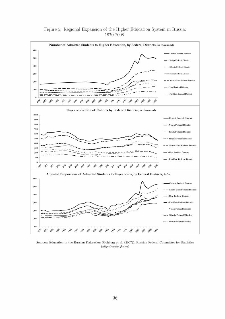
Figure 5: Regional Expansion of the Higher Education System in Russia:1970-2008
0
100
200
300
400
500
600
700
800
900
1000
17-year-olds: Size of Cohorts by Federal Districts, in thousands
Central Federal District
Volga Federal District
South Federal District
Siberia Federal District
North-West Federal District
Ural Federal District
Far-East Federal District
0
100
200
300
400
500
600
Number of Admitted Students to Higher Education, by Federal Districts, in thousands
Central Federal District
Volga Federal District
Siberia Federal District
South Federal District
North-West Federal District
Ural Federal District
Far-East Federal District
0%
10%
20%
30%
40%
50%
60%
Adjusted Proportions of Admitted Students to 17-year-olds, by Federal Districts, in %
Central Federal District
North-West Federal District
Ural Federal District
Far-East Federal District
Volga Federal District
Siberia Federal District
South Federal District
Sources: Education in the Russian Federation (Gohberg et al. (2007)), Russian Federal Committee for Statistics
(http://www.gks.ru)
36
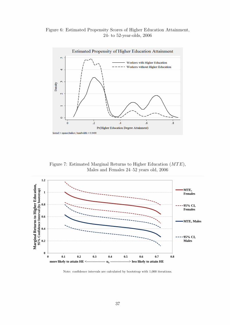
Figure 6: Estimated Propensity Scores of Higher Education Attainment,24- to 52-year-olds, 2006
Figure 7: Estimated Marginal Returns to Higher Education (MTE),Males and Females 24–52 years old, 2006
0
0.2
0.4
0.6
0.8
1
1.2
0 0.1 0.2 0.3 0.4 0.5 0.6 0.7 0.8
Mar
gina
l Ret
urns
to H
ighe
r E
duca
tion,
95
% C
onfid
ence
Inte
rval
(by
boot
stra
p)
more likely to attain HE <----------------- uS -----------------> less likely to attain HE
MTE,Females
95% CI,Females
MTE, Males
95% CI,Males
Note: confidence intervals are calculated by bootstrap with 1,000 iterations.
37
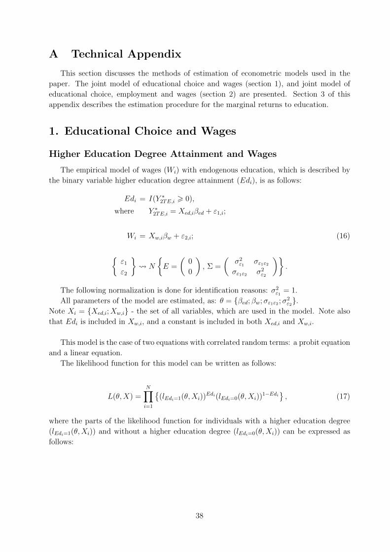
A Technical Appendix
This section discusses the methods of estimation of econometric models used in the
paper. The joint model of educational choice and wages (section 1), and joint model of
educational choice, employment and wages (section 2) are presented. Section 3 of this
appendix describes the estimation procedure for the marginal returns to education.
1. Educational Choice and Wages
Higher Education Degree Attainment and Wages
The empirical model of wages (Wi) with endogenous education, which is described by
the binary variable higher education degree attainment (Edi), is as follows:
Edi = I(Y ∗2TE,i > 0),
where Y ∗2TE,i = Xed,iβed + ε1,i;
Wi = Xw,iβw + ε2,i; (16)
{ε1
ε2
} N
{E =
(0
0
), Σ =
(σ2ε1
σε1ε2σε1ε2 σ2
ε2
)}.
The following normalization is done for identification reasons: σ2ε1
= 1.
All parameters of the model are estimated, as: θ = {βed; βw;σε1ε2 ;σ2ε2}.
Note Xi = {Xed,i;Xw,i} - the set of all variables, which are used in the model. Note also
that Edi is included in Xw,i, and a constant is included in both Xed,i and Xw,i.
This model is the case of two equations with correlated random terms: a probit equation
and a linear equation.
The likelihood function for this model can be written as follows:
L(θ,X) =N∏i=1
{(lEdi=1(θ,Xi))
Edi(lEdi=0(θ,Xi))1−Edi
}, (17)
where the parts of the likelihood function for individuals with a higher education degree
(lEdi=1(θ,Xi)) and without a higher education degree (lEdi=0(θ,Xi)) can be expressed as
follows:
38
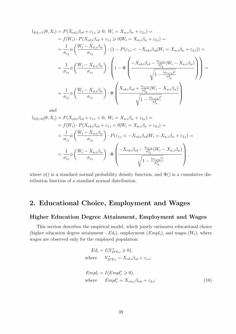
lEdi=1(θ,Xi) = P (Xed,iβed + ε1,i > 0; Wi = Xw,iβw + ε2,i) =
= f(Wi) · P (Xed,iβed + ε1,i > 0|Wi = Xw,iβw + ε2,i) =
=1
σε2φ
(Wi −Xw,iβw
σε2
)· (1− P (ε1,i < −Xed,iβed|Wi = Xw,iβw + ε2,i)) =
=1
σε2φ
(Wi −Xw,iβw
σε2
)·
1− Φ
−Xed,iβed −σε1ε2σ2ε2
(Wi −Xw,iβw)√1− (σε1ε2 )2
σ2ε2
=
=1
σε2φ
(Wi −Xw,iβw
σε2
)· Φ
Xed,iβed +σε1ε2σ2ε2
(Wi −Xw,iβw)√1− (σε1ε2 )2
σ2ε2
and
lEdi=0(θ,Xi) = P (Xed,iβed + ε1,i < 0; Wi = Xw,iβw + ε2,i) =
= f(Wi) · P (Xed,iβed + ε1,i < 0|Wi = Xw,iβw + ε2,i) =
=1
σε2φ
(Wi −Xw,iβw
σε2
)· P (ε1,i < −Xed,iβed|Wi = Xw,iβw + ε2,i) =
=1
σε2φ
(Wi −Xw,iβw
σε2
)· Φ
−Xed,iβed −σε1ε2σ2ε2
(Wi −Xw,iβw)√1− (σε1ε2 )2
σ2ε2
,
where φ() is a standard normal probability density function, and Φ() is a cumulative dis-
tribution function of a standard normal distribution.
2. Educational Choice, Employment and Wages
Higher Education Degree Attainment, Employment and Wages
This section describes the empirical model, which jointly estimates educational choice
(higher education degree attainment - Edi), employment (Empli), and wages (Wi), where
wages are observed only for the employed population:
Edi = I(Y ∗2TE,i > 0),
where Y ∗2TE,i = Xed,iβed + ε1,i;
Empli = I(Empl∗i > 0),
where Empl∗i = Xem,iβem + ε2,i; (18)
39
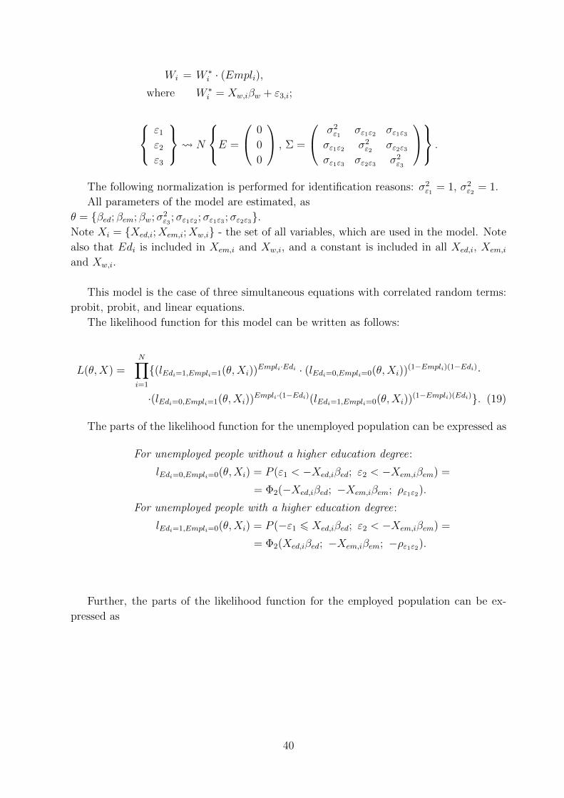
Wi = W ∗i · (Empli),
where W ∗i = Xw,iβw + ε3,i;
ε1
ε2
ε3
N
E =
0
0
0
, Σ =
σ2ε1
σε1ε2 σε1ε3σε1ε2 σ2
ε2σε2ε3
σε1ε3 σε2ε3 σ2ε3
.
The following normalization is performed for identification reasons: σ2ε1
= 1, σ2ε2
= 1.
All parameters of the model are estimated, as
θ = {βed; βem; βw;σ2ε3
;σε1ε2 ;σε1ε3 ;σε2ε3}.Note Xi = {Xed,i;Xem,i;Xw,i} - the set of all variables, which are used in the model. Note
also that Edi is included in Xem,i and Xw,i, and a constant is included in all Xed,i, Xem,i
and Xw,i.
This model is the case of three simultaneous equations with correlated random terms:
probit, probit, and linear equations.
The likelihood function for this model can be written as follows:
L(θ,X) =N∏i=1
{(lEdi=1,Empli=1(θ,Xi))Empli·Edi · (lEdi=0,Empli=0(θ,Xi))
(1−Empli)(1−Edi)·
·(lEdi=0,Empli=1(θ,Xi))Empli·(1−Edi)(lEdi=1,Empli=0(θ,Xi))
(1−Empli)(Edi)}. (19)
The parts of the likelihood function for the unemployed population can be expressed as
For unemployed people without a higher education degree:
lEdi=0,Empli=0(θ,Xi) = P (ε1 < −Xed,iβed; ε2 < −Xem,iβem) =
= Φ2(−Xed,iβed; −Xem,iβem; ρε1ε2).
For unemployed people with a higher education degree:
lEdi=1,Empli=0(θ,Xi) = P (−ε1 6 Xed,iβed; ε2 < −Xem,iβem) =
= Φ2(Xed,iβed; −Xem,iβem; −ρε1ε2).
Further, the parts of the likelihood function for the employed population can be ex-
pressed as
40

For employed people without a higher education degree:
lEdi=0,Empli=1(θ,Xi) = P (ε1 < −Xed,iβed; −ε2 < Xem,iβem; Wi = Xw,iβw + ε3,i) =
= f(Wi) · P (ε1 < −Xed,iβed; −ε2 < Xem,iβem| Wi = Xw,iβw + ε3,i) =
=1
σε3φ
(Wi −Xw,iβw
σε3
)·
·Φ2
−Xed,iβed −σε1ε3σ2ε3
· (Wi −Xw,iβw)√σ2ε1− σ2
ε1ε3
σ2ε3
;Xem,iβem +
σε2ε3σ2ε3
· (Wi −Xw,iβw)√σ2ε2− σ2
ε2ε3
σ2ε3
; −ρ(1,2|3)
,
where: ρ(1,2|3) =σε1ε2 −
σε1ε3 ·σε2ε3σ2ε3√
(σ2ε1− σ2
ε1ε3
σ2ε3
)(σ2ε2− σ2
ε2ε3
σ2ε3
)
;
For employed people with a higher education degree:
lEdi=1,Empli=1(θ,Xi) = P (−ε1 6 Xed,iβed; −ε2 < Xem,iβem; Wi = Xw,iβw + ε3,i) =
= f(Wi) · P (−ε1 6 Xed,iβed; −ε2 < Xem,iβem| Wi = Xw,iβw + ε3,i) =
=1
σε3φ
(Wi −Xw,iβw
σε3
)·
·Φ2
Xed,iβed +σε1ε3σ2ε3
· (Wi −Xw,iβw)√σ2ε1− σ2
ε1ε3
σ2ε3
;Xem,iβem +
σε2ε3σ2ε3
· (Wi −Xw,iβw)√σ2ε2− σ2
ε2ε3
σ2ε3
; ρ(1,2|3)
,
where: ρ(1,2|3) =σε1ε2 −
σε1ε3 ·σε2ε3σ2ε3√
(σ2ε1− σ2
ε1ε3
σ2ε3
)(σ2ε2− σ2
ε2ε3
σ2ε3
)
.
Φ2(a1; a2; ρ) is a joint cumulative distribution function for the two bivariate normally
distributed variables with means = 0, variations = 1, and correlation ρ.
41
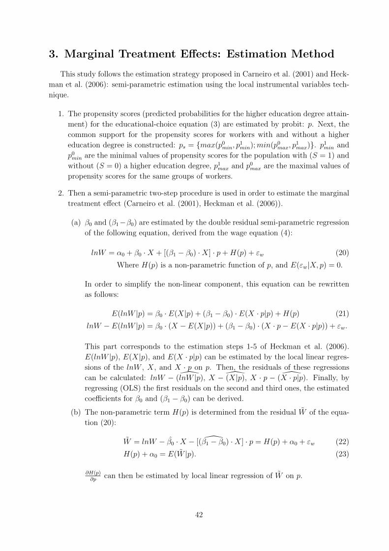
3. Marginal Treatment Effects: Estimation Method
This study follows the estimation strategy proposed in Carneiro et al. (2001) and Heck-
man et al. (2006): semi-parametric estimation using the local instrumental variables tech-
nique.
1. The propensity scores (predicted probabilities for the higher education degree attain-
ment) for the educational-choice equation (3) are estimated by probit: p. Next, the
common support for the propensity scores for workers with and without a higher
education degree is constructed: ps = {max(p0min, p
1min);min(p0
max, p1max)}. p1
min and
p0min are the minimal values of propensity scores for the population with (S = 1) and
without (S = 0) a higher education degree, p1max and p0
max are the maximal values of
propensity scores for the same groups of workers.
2. Then a semi-parametric two-step procedure is used in order to estimate the marginal
treatment effect (Carneiro et al. (2001), Heckman et al. (2006)).
(a) β0 and (β1−β0) are estimated by the double residual semi-parametric regression
of the following equation, derived from the wage equation (4):
lnW = α0 + β0 ·X + [(β1 − β0) ·X] · p+H(p) + εw (20)
Where H(p) is a non-parametric function of p, and E(εw|X, p) = 0.
In order to simplify the non-linear component, this equation can be rewritten
as follows:
E(lnW |p) = β0 · E(X|p) + (β1 − β0) · E(X · p|p) +H(p) (21)
lnW − E(lnW |p) = β0 · (X − E(X|p)) + (β1 − β0) · (X · p− E(X · p|p)) + εw.
This part corresponds to the estimation steps 1-5 of Heckman et al. (2006).
E(lnW |p), E(X|p), and E(X · p|p) can be estimated by the local linear regres-
sions of the lnW , X, and X · p on p. Then, the residuals of these regressions
can be calculated: lnW − ̂(lnW |p), X − (̂X|p), X · p − ̂(X · p|p). Finally, by
regressing (OLS) the first residuals on the second and third ones, the estimated
coefficients for β0 and (β1 − β0) can be derived.
(b) The non-parametric term H(p) is determined from the residual W̃ of the equa-
tion (20):
W̃ = lnW − β̂0 ·X − [(β̂1 − β0) ·X] · p = H(p) + α0 + εw (22)
H(p) + α0 = E(W̃ |p). (23)
∂H(p)∂p
can then be estimated by local linear regression of W̃ on p.
42
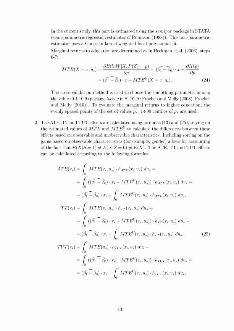
In the current study, this part is estimated using the semipar package in STATA
(semi-parametric regression estimator of Robinson (1988)). This non-parametric
estimator uses a Gaussian kernel weighted local polynomial fit.
Marginal returns to education are determined as in Heckman et al. (2006), steps
6-7:
MTE(X = x, us) =∂E(lnW |X,P (Z) = p)
∂p= (β̂1 − β0) · x+
∂H(p)
∂p
= (β̂1 − β0) · x+MTEU(X = x, us). (24)
The cross-validation method is used to choose the smoothing parameter among
the values 0.1÷0.9 (package locreg in STATA: Froelich and Melly (2008), Froelich
and Melly (2010)). To evaluate the marginal returns to higher education, the
evenly spaced points of the set of values ps: 1÷99 centiles of ps are used.
3. The ATE, TT and TUT effects are calculated using formulas (13) and (25), relying on
the estimated values of MTE and MTEU to calculate the differences between these
effects based on observable and unobservable characteristics. Including sorting on the
gains based on observable characteristics (for example, gender) allows for accounting
of the fact that E(X|S = 1) 6= E(X|S = 0) 6= E(X). The ATE, TT and TUT effects
can be calculated according to the following formulas:
ATE(xi) =
∫ 1
0
MTE(xi, us) · hATE(xi, us) dus =
=
∫ 1
0
((β̂1 − β0) · xi +MTEU(xi, us)) · hATE(xi, us) dus =
= (β̂1 − β0) · xi +
∫ 1
0
MTEU(xi, us) · hATE(xi, us) dus,
TT (xi) =
∫ 1
0
MTE(xi, us) · hTT (xi, us) dus =
=
∫ 1
0
((β̂1 − β0) · xi +MTEU(xi, us)) · hTT (xi, us) dus =
= (β̂1 − β0) · xi +
∫ 1
0
MTEU(xi, us) · hTT (xi, us) dus, (25)
TUT (xi) =
∫ 1
0
MTE(us) · hTUT (xi, us) dus =
=
∫ 1
0
((β̂1 − β0) · xi +MTEU(xi, us)) · hTUT (xi, us) dus =
= (β̂1 − β0) · xi +
∫ 1
0
MTEU(xi, us) · hTUT (xi, us) dus,
43

where the weights are
hATE(xi, us) = 1,
hTT (xi, us) =Pr(P (Z) > us|X = xi)∫ 1
0Pr(P (Z) > us|X = xi) dus
,
hTUT (xi, us) =Pr(P (Z) < us|X = xi)∫ 1
0Pr(P (Z) < us|X = xi) dus
.
ATE =
∫X
ATE(xi) dFX(x) =
=
∫X
(β̂1 − β0) · xi dFX(x) +
∫X
∫ 1
0
MTEU(xi, us) · hATE(xi, us) dus dFX(x) =
= (β̂1 − β0) · E(X) + E(MTEU), (26)
TT =
∫X|S=1
TT (xi) dFX|S=1(x) =
=
∫X|S=1
(β̂1 − β0) · xi dFX|S=1(x) +
+
∫X|S=1
∫ 1
0
MTEU(xi, us) · hTT (xi, us) dus dFX|S=1(x) =
= (β̂1 − β0) · E(X|S = 1) + E(MTEU · hTT |S = 1), (27)
TUT =
∫X|S=0
TUT (xi) dFX|S=0(x) =
=
∫X|S=0
(β̂1 − β0) · xi dFX|S=0(x) +
+
∫X|S=0
∫ 1
0
MTEU(xi, us) · hTUT (xi, us) dus dFX|S=0(x) =
= (β̂1 − β0) · E(X|S = 0) + E(MTEU · hTUT |S = 0). (28)
4. Finally, a bootstrap is used to calculate the variance and t-statistics for the esti-
mated effects of ATE, TT and TUT, and the 95% confidence interval for the MTE
estimations.
44