expected utility vs. equivalent monetary value · inference in ghostbusters a ghost is in the grid...
TRANSCRIPT

Expected Utility vs. Equivalent Monetary Value
▪ If utility function is U($x) = x2 , given a lottery L = [0.5, $0; 0.5, $40] ▪ Expected Utility: EU(L) = ? (answer: 800)
▪ Equivalent Monetary Value is the amount of money you would pay in exchange for the lottery. EMV(L) = ? (answer: $28.284)
0 40 x2 0 1600

What Utilities to Use?
▪ For worst-case minimax reasoning, terminal function scale doesn’t matter ▪ We just want better states to have higher evaluations (get the ordering right) ▪ We call this insensitivity to monotonic transformations
▪ For average-case expectimax reasoning, we need magnitudes to be meaningful
0 40 20 30 x2 0 1600 400 900

What Utilities to Use?
0 40 20 30 x2 0 1600 400 900
▪ For worst-case minimax reasoning, terminal function scale doesn’t matter ▪ We just want better states to have higher evaluations (get the ordering right) ▪ We call this insensitivity to monotonic transformations
▪ For average-case expectimax reasoning, we need magnitudes to be meaningful

CS 5522: Artificial Intelligence II Hidden Markov Models
Instructor: Wei Xu
Ohio State University [These slides were adapted from CS188 Intro to AI at UC Berkeley.]

Probability Recap
▪ Conditional probability
▪ Product rule
▪ Chain rule
▪ X, Y independent if and only if:
▪ X and Y are conditionally independent given Z if and only if:

Probabilistic Inference
▪ Probabilistic inference: compute a desired probability from other known probabilities (e.g. conditional from joint)
▪ We generally compute conditional probabilities ▪ P(on time | no reported accidents) = 0.90 ▪ These represent the agent’s beliefs given the evidence
▪ Probabilities change with new evidence: ▪ P(on time | no accidents, 5 a.m.) = 0.95 ▪ P(on time | no accidents, 5 a.m., raining) = 0.80 ▪ Observing new evidence causes beliefs to be updated

Inference in Ghostbusters▪ A ghost is in the grid
somewhere ▪ Sensor readings tell how
close a square is to the ghost ▪ On the ghost: red ▪ 1 or 2 away: orange ▪ 3 or 4 away: yellow ▪ 5+ away: green
P(red | 3) P(orange | 3) P(yellow | 3) P(green | 3)
0.05 0.15 0.5 0.3
▪ Sensors are noisy, but we know P(Color | Distance)
[Demo: Ghostbuster – no probability (L12D1) ]

Video of Demo Ghostbuster – No probability

Uncertainty
▪ General situation:
▪ Observed variables (evidence): Agent knows certain things about the state of the world (e.g., sensor readings or symptoms)
▪ Unobserved variables: Agent needs to reason about other aspects (e.g. where an object is or what disease is present)
▪ Model: Agent knows something about how the known variables relate to the unknown variables
▪ Probabilistic reasoning gives us a framework for managing our beliefs and knowledge

Video of Demo Ghostbusters with Probability

Hidden Markov Models

Hidden Markov Models
▪ Markov chains not so useful for most agents ▪ Need observations to update your beliefs
▪ Hidden Markov models (HMMs) ▪ Underlying Markov chain over states X ▪ You observe outputs (effects) at each time step
X5X2
E1
X1 X3 X4
E2 E3 E4 E5

Example: Weather HMM
Rt Rt+1 P(Rt+1|Rt)
+r +r 0.7
+r -r 0.3
-r +r 0.3
-r -r 0.7
Umbrellat-1
Rt Ut P(Ut|Rt)
+r +u 0.9
+r -u 0.1
-r +u 0.2
-r -u 0.8
Umbrellat Umbrellat+1
Raint-1 Raint Raint+1
▪ An HMM is defined by: ▪ Initial distribution: ▪ Transitions: ▪ Emissions:

Example: Ghostbusters HMM
▪ P(X1) = uniform
▪ P(X|X’) = usually move clockwise, but sometimes move in a random direction or stay in place
▪ P(Rij|X) = same sensor model as before: red means close, green means far away.
1/9 1/9
1/9 1/9
1/9
1/9
1/9 1/9 1/9
P(X1)
P(X|X’=<1,2>)
1/6 1/6
0 1/6
1/2
0
0 0 0
X5
X2
Ri,j
X1 X3 X4
Ri,j Ri,j Ri,j
[Demo: Ghostbusters – Circular Dynamics – HMM (L14D2)]

Video of Demo Ghostbusters – Circular Dynamics -- HMM

Joint Distribution of an HMM
▪ Joint distribution:
▪ More generally:
▪ Questions to be resolved: ▪ Does this indeed define a joint distribution? ▪ Can every joint distribution be factored this way, or are we making some assumptions
about the joint distribution by using this factorization?
X5X2
E1
X1 X3
E2 E3 E5

▪ From the chain rule, every joint distribution over can be written as:
▪ Assuming that
gives us the expression posited on the previous slide:
X2
E1
X1 X3
E2 E3
Chain Rule and HMMs

Chain Rule and HMMs
▪ From the chain rule, every joint distribution over can be written as:
▪ Assuming that for all t: ▪ State independent of all past states and all past evidence given the previous state, i.e.:
▪ Evidence is independent of all past states and all past evidence given the current state, i.e.:
gives us the expression posited on the earlier slide:
X2
E1
X1 X3
E2 E3

Implied Conditional Independencies
▪ Many implied conditional independencies, e.g.,
▪ To prove them ▪ Approach 1: follow similar (algebraic) approach to what we did in the Markov
models lecture ▪ Approach 2: directly from the graph structure (3 lectures from now)
▪ Intuition: If path between U and V goes through W, then
X2
E1
X1 X3
E2 E3
[Some fineprint later]
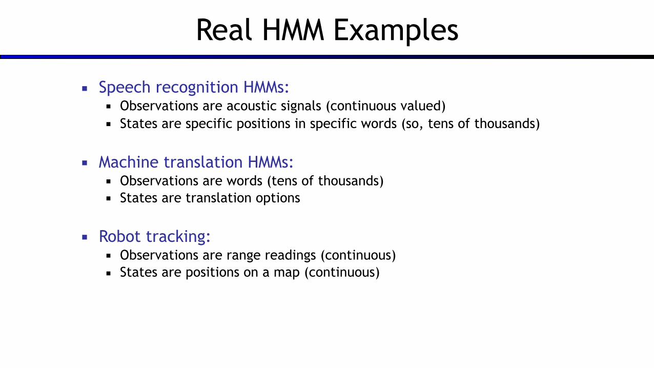
Real HMM Examples
▪ Speech recognition HMMs: ▪ Observations are acoustic signals (continuous valued) ▪ States are specific positions in specific words (so, tens of thousands)
▪ Machine translation HMMs: ▪ Observations are words (tens of thousands) ▪ States are translation options
▪ Robot tracking: ▪ Observations are range readings (continuous) ▪ States are positions on a map (continuous)

Filtering / Monitoring
▪ Filtering, or monitoring, is the task of tracking the distribution Bt(X) = Pt(Xt | e1, …, et) (the belief state) over time
▪ We start with B1(X) in an initial setting, usually uniform
▪ As time passes, or we get observations, we update B(X)
▪ The Kalman filter was invented in the 60’s and first implemented as a method of trajectory estimation for the Apollo program

Example: Robot Localization
t=0 Sensor model: can read in which directions there is a wall, never
more than 1 mistake Motion model: may not execute action with small prob.
10Prob
Example from Michael Pfeiffer
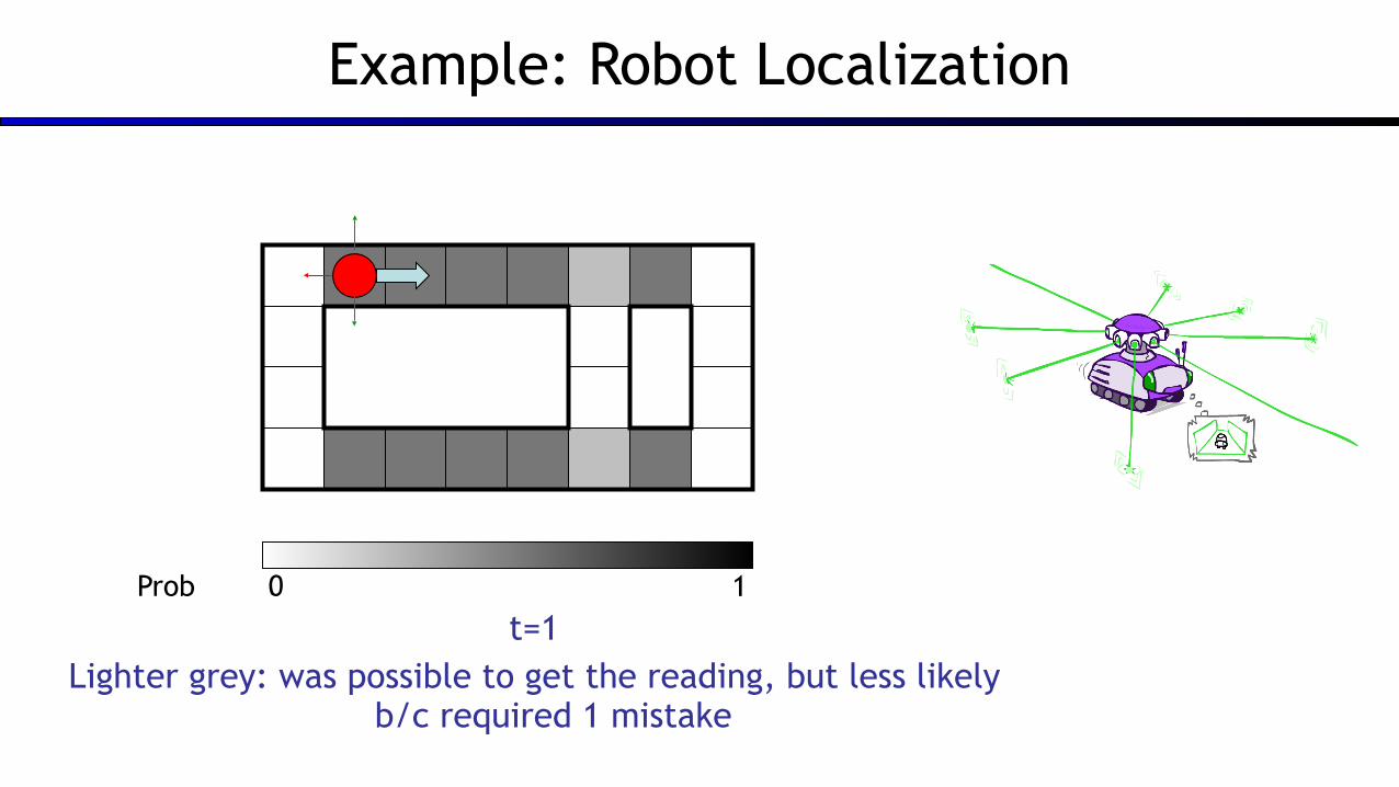
Example: Robot Localization
t=1 Lighter grey: was possible to get the reading, but less likely
b/c required 1 mistake
10Prob

Example: Robot Localization
t=2
10Prob

Example: Robot Localization
t=3
10Prob

Example: Robot Localization
t=4
10Prob

Example: Robot Localization
t=5
10Prob

Inference: Base Cases
E1
X1
X2X1

Passage of Time
▪ Assume we have current belief P(X | evidence to date)
▪ Then, after one time step passes:
▪ Basic idea: beliefs get “pushed” through the transitions ▪ With the “B” notation, we have to be careful about what time step t the belief is about, and
what evidence it includes
X2X1
▪ Or compactly:

Example: Passage of Time
▪ As time passes, uncertainty “accumulates”
T = 1 T = 2 T = 5
(Transition model: ghosts usually go clockwise)

Observation▪ Assume we have current belief P(X | previous evidence):
▪ Then, after evidence comes in:
▪ Or, compactly:
E1
X1
▪ Basic idea: beliefs “reweighted” by likelihood of evidence
▪ Unlike passage of time, we have to renormalize

Example: Observation
▪ As we get observations, beliefs get reweighted, uncertainty “decreases”
Before observation After observation

Example: Weather HMM
Rt Rt+1 P(Rt+1|Rt)
+r +r 0.7
+r -r 0.3
-r +r 0.3
-r -r 0.7
Rt Ut P(Ut|Rt)
+r +u 0.9
+r -u 0.1
-r +u 0.2
-r -u 0.8
Umbrella1 Umbrella2
Rain0 Rain1 Rain2
B(+r) = 0.5 B(-r) = 0.5
B’(+r) = 0.5 B’(-r) = 0.5
B(+r) = 0.818 B(-r) = 0.182
B’(+r) = 0.627 B’(-r) = 0.373
B(+r) = 0.883 B(-r) = 0.117

The Forward Algorithm▪ We are given evidence at each time and want to know
▪ We can derive the following updatesWe can normalize as we go if we want to have P(x|e) at each time
step, or just once at the end…

Online Belief Updates
▪ Every time step, we start with current P(X | evidence) ▪ We update for time:
▪ We update for evidence:
▪ The forward algorithm does both at once (and doesn’t normalize)
X2X1
X2
E2

Pacman – Sonar (P4)
[Demo: Pacman – Sonar – No Beliefs(L14D1)]

Video of Demo Pacman – Sonar (no beliefs)

Pacman – Sonar (P4)
[Demo: Pacman – Sonar – No Beliefs(L14D1)]

Video of Demo Pacman – Sonar (with beliefs)

Next Time: Particle Filtering and Applications of HMMs