WP/06/165

Expenditure Composition and Distortionary Tax for Equitable Economic Growth

Hyun Park

© 2006 International Monetary Fund WP/06/165

IMF Working Paper

Fiscal Affairs Department

Expenditure Composition and Distortionary Tax for Equitable Economic Growth

Prepared by Hyun Park1

Authorized for distribution by Sanjeev Gupta

June 2006

Abstract

This Working Paper should not be reported as representing the views of the IMF. The views expressed in this Working Paper are those of the author(s) and do not necessarily represent those of the IMF or IMF policy. Working Papers describe research in progress by the author(s) and are published to elicit comments and to further debate.

This paper continues the study of optimal fiscal policy in a growing economy by exploring a case in which the government simultaneously provides three main categories of expenditures with distortionary tax finance: public production services, public consumption services, and state-contingent redistributive transfers. The paper shows that in a general equilibrium modelwith given exogenous fiscal policy, a nonlinear relation exists between the suboptimal long-run growth rate in a competitive economy and distortionary tax rates. When fiscal policy is endogenously chosen at a social optimum, the relation between the rate of growth and tax rates is always negative. These two conclusions suggest that the interaction between fiscal policy and growth may be complicated enough that it cannot be captured in a simple linear model using an aggregate measure of fiscal policy. The sources of nonlinearity include expectation and coordination of fiscal policy, impluse response of government policies, and the presence of positive externality due to government spending. JEL Classification Numbers: E62, H50, O40 Keywords: allocative and redistributive policy, endogeneity, nonlinearity Author(s) E-Mail Address: econhyun@khu.ac.kr 1 I would like to thank D. Coady, K. Chu, S. Gupta, B. Clements, A. Philippopoulos, and S. Tareq for discussions and comments. I also wish to thank C. Wu and K. Angelopoulos for their help in the empirical analysis of this paper. I completed the paper while visiting the Fiscal Affairs Department of the International Monetary Fund, and I am grateful for the hospitality. All remaining errors are mine.

- 2 -

Contents Page

I. Introduction ............................................................................................................................3

II. The Decentralized Competitive Equilibrium ........................................................................5 A. The Role of Economic Policies.................................................................................6 B. The Problem of Households......................................................................................7 C. The Problem of the Firm ...........................................................................................8 D. Decentralized Competitive Equilibrium with Exogenous Government Policies......8

III. Ramsey Optimal Policy and Equilibrium ..........................................................................12 A. Properties of Economic Policy along the Optimal Equilibrium Path .....................13 B. A Special Case with No Consumptive Expenditure................................................15 C. Symmetric Long-Run Equilibrium..........................................................................16

IV. Empirical Observations .....................................................................................................18

V. Concluding Remarks...........................................................................................................28

Tables 1. Growth Regressions: A Nonlinear Effect of Tax Revenues on the Growth Rate................21 2. Correlations between the (effective) Tax Rate and the Fraction of Productive Government Spending (theta) for 26 OECD Countries................................................................................24 3. Correlations between the Growth Rate and the Income Redistribution (sigma) for 25 OECD Countries ......................................................................................................................25 4. Correlations between Redistributive Government Spending (RGS) and Income Inequality (Gini) for 25 OECD Countries.................................................................................................26 5. Correlations between the Income Redistribution (sigma) and the Variance of GDP for 25 OECD Countries ......................................................................................................................27

Figures 1. Growth Rates and Exogenous Fiscal Policy ........................................................................11 2. Tax Rate and Share of Productive Spending with Endogenous Fiscal Policy.....................18 3. Tax Rate and the Fraction of Productive Government Spending ........................................23 4. Income Redistribution Parameter and the Growth Rate ......................................................25 5. Redistributive Government Spending and Income Inequality.............................................26 6. Income Redistribution Parameter and GDP Variance .........................................................27

Appendices I. The Decentralized Competitive Equilibrium with Exogenous Policies ...............................29 II. The Ramsey Optimal Equilibrium with Endogenous Policies............................................30 III. The Symmetric Ramsey Equilibrium.................................................................................31 IV. The Long-Run Ramsey Equilibrium .................................................................................32

References................................................................................................................................33

- 3 -

I. INTRODUCTION

The effect of government policies on economic performance and welfare is one of the oldest, most studied, and most controversial topics in economics. Functions assigned to a government include protecting property rights, enforcing contracts, correcting externalities, and providing public goods. In a more extended role, a government also redistributes wealth and income, provides social security, and stabilizes and regulates the economy. Most studies choose a set of limited government functions when examining governmental influence on economic variables. For example, the allocative and redistributive roles of the government are studied separately in the examination of the relation between equity and growth; however, this separation ignores the potential importance of interaction among policy instruments. In fact, the vast scope of policy instruments works to promote simultaneously both higher economic growth and greater equity. This paper develops a dynamic general equilibrium model for understanding the range of economic structures and policy instruments. In particular, the paper examines the effects of government policy instruments on promoting economic growth and improving income equality by explicitly considering the composition of expenditures and taxation. The paper also investigates the impact of taxes and expenditure composition on economic growth and equity using a common specification of cross-country regressions. A large body of theoretical and empirical studies has been devoted to understanding the effects of fiscal policy on economic growth. Unlike a Solow-type, neoclassical growth model, fiscal policy can affect long-run growth in endogenous growth models with productive government spending (e.g., Barro, 1990; Jones, Manuelli, and Rossi, 1993; Stokey and Rebelo, 1993; Lucas, 1989). Many results in these theoretical models have been studied empirically (e.g., Barro, 1991; Mankiw, Romer, and Weil, 1992; Levine and Renelt, 1992; Easterly and Rebelo, 1993; Barro and Sala-i-Martin, 1992, 2004; Jones, 1995; Devarajan, Swaroop, and Zou, 1996). Other empirical studies (e.g., Kneller, Bleaney, and Gemmell, 1999; Bleaney, Gemmell, and Kneller, 2001; Alesina and Perotti, 1995, 1997; Giavazzi, Jappelli, and Pagano, 2000; Gupta and others, 2002) have extended these studies by examining the composition of both government expenditure and taxation. Also, models exist of endogenizing fiscal policy instruments that include redistributive policy by political process (e.g., Persson and Tabellini, 1994; Alesina and Rodrik, 1994; Krusell, Quadrini, and Rios-Rull, 1997). Peltzman (1980) and Buchanan and Wagner (1977) studied the relation between recent rapid growth of a government and the incentive to redistribute income and wealth by separating these variables from demand for public goods. Political economy models (e.g., Benabou, 1996) predict a negative relation between growth and economic inequality through redistributive political pressure. Galor and Tsiddon (1997) and Forbes (2000) developed theories that indicate that inequality and growth are positively related. In addition, Benabou (2000) and de Mello and Tiongson (2003) reported a nonlinear relation between inequality and growth. In this paper, I consider a simple dynamic general equilibrium model with both exogenous and endogenous fiscal policies. This model is a simple extension of Barro’s (1990) model for

- 4 -

productive government spending with endogenous growth.2 According to this model, many households and firms interact with a government. Fiscal policy consists of an income tax policy and three expenditure programs: consumptive spending, productive spending, and income transfer. Consumptive government spending increases a household’s utility directly, and productive spending provides positive externalities to private firms. Income transfer is provided to individuals who own less than the average capital in the economy. In this model, productive government service is an engine of long-run growth, and consumptive spending and income transfer play a role in equitable economic growth. The main focus of this paper is to study the effects of fiscal policy on economic growth and income equality in a growing economy. As previously stated, a government simultaneously provides consumptive, productive, and redistributive spending. That is, I explicitly decompose allocative and redistributive government activities. I then consider the relation between a particular policy instrument and economic growth when a set of policy instruments is chosen both exogenously and endogenously. When fiscal policy is endogenously determined, I also consider implementation conditions for a decentralized competitive economy. I am especially interested in the productivity associated with each policy instrument among the four categories of fiscal policy, as well as the net cost and benefit of government activities in terms of economic growth. I also explain the source of fragile empirical results of endogenous growth models by focusing on theoretical investigation of composition of government expenditure (e.g., Kneller, Bleaney, and Gemmell, 1999; Levine and Renelt, 1992; Mueller, 2003). My analysis shows that an inverse U-shaped relationship exists between tax rates and growth rates when the fiscal policy is exogenous.3 However, when fiscal policy is endogenously chosen at a social optimum, the relation between the growth rate and tax rates is always negative. That is, the nonlinear hump relation between growth and taxes disappears.4 These two results imply that the different properties of exogenous and endogenous fiscal policy theoretically account for the difference in the relation between growth and fiscal policy in empirical studies. As argued by Cooley and LeRoy (1981), these differences show how empirical studies for growth and fiscal policies critically depend on the choice of independent policy variables in growth regressions. In addition, an alternative decomposition of government spending may affect the response of private sector investment to fiscal policy (see Levine and Renelt, 1992; Alesina and Perotti, 1995; Devarajan, Swaroop, and Zou, 1996; Giavazzi, Jappelli, and Pagano, 2000).

2 Kneller, Bleany, and Gemmell (1999) pointed out that those who focus either on expenditure or taxation of a government’s budget suffer from systematic biases in their estimates in a general equilibrium model. 3 This nonlinear relation is common in the growth literature (e.g., Devarajan, Swaroop, and Zou, 1996; Alesina and Rodrik, 1994; Eicher and Garcia-Penalosa, 2001; Bourguignon and Morrisson, 1998). 4 See Devarajan, Swaroop, and Zou (1996) for empirical evidence of a negative relationship between productive spending and output growth. Also, Alesina and others (2002) shows that fiscal policy negatively influences labor cost, profit, and, thus, investment.

- 5 -

This problem is fundamental for the identification of exogenous and endogenous variables in empirical studies in endogenous growth models.5 This paper demonstrates simple empirical evidence for the difference between exogenous and endogenous fiscal policy in cross-country data. As in exogenous fiscal policies, fiscal policy (here, income tax rates) has a nonlinear effect on the growth rate. For this regression analysis, I also include rent-seeking variables (e.g., Barro, 1991; Mauro, 1995; Barro and Sala-i-Martin, 2004). The statistical significance of an index of rent-seeking activities, including regional dummies, implies that a government’s implementation abilities conditionally affect economic growth and income distribution. I also find a negative association between the growth rate and income redistribution, which is consistent with political economy literature (Benhabib and Rustichini, 1996), along with a negative relation between consumptive spending and income inequality (Chu, Davoodi, and Gupta, 2004). In addition, as expected both in endogenous and exogenous policies, I find a negative relation between tax rates and productive government spending (see Section III.2 and Table 2). The remainder of the paper is organized as follows: Section II presents a simple endogenous growth model and examines a decentralized competitive economy with exogenous fiscal policy. Section III solves and characterizes a socially optimal equilibrium and, thus, examines the relation between long-run growth rates and income tax rates. Section IV illustrates empirical observation on the relation between fiscal policy and growth. Finally, Section V provides some concluding remarks.

II. THE DECENTRALIZED COMPETITIVE EQUILIBRIUM

I consider a simple dynamic general equilibrium model. The decentralized closed economy consists of an infinite number of households and firms and a government. Households purchase goods for consumption and save in the form of assets. Firms produce goods with the use of capital and labor and make rental payments to the owners of capital.6 For simplicity, all firms are identical. The government imposes taxes on household incomes to finance public production services, public consumption services, and transfer payments.7 I assume perfect foresight and no population growth on an infinite horizon.

5 The methodological issue in empirical studies for endogenous growth models is also discussed in Slemrod, Gale, and Easterly (1995). In addition, Levine and Renelt (1992) attributed nonrobustness of empirical findings to inadequate measures of the effects of public goods and failure to capture characteristics of a tax system. 6 For simplicity, I assume households supply inelastically a fixed amount of labor services. However, the results may change if households make endogenous labor/leisure choices (see Alesina and Rodrik, 1994; Turnovsky and Fisher, 1995). 7 Thus, following Barro (1990), the engine of long-term growth is public production services; in Glomm and Ravikumar (1992) and Perotti (1993), the engine is human capital. See also Fernandez and Rogerson (1995) for human capital and redistribution.

- 6 -

A. The Role of Economic Policies

It is convenient to start with the role of economic policy. The government receives tax revenues ])([ wLira +τ from each household i , ],0[ Ii∈ , where 10 <≤ τ is the tax rate on household i ’s

income, w is the market wage rate, L is labor supply, r is the market return to asset, and )(ia is household i ’s asset at the beginning of each period. The government uses its total tax revenues,

∫ +I

diwLira0

])([τ , to finance the provision of aggregate public production services, G , aggregate

public consumption services, H , and transfer payments to households, ∫I

dii0

)(σ , where )(iσ is a

transfer payment received by each household i . Thus, at each instant of time, the government budget constraint is:

=++ ∫I

diiHG0

)(σ ∫ +I

diwLira0

])([τ .8

This government budget constraint can be decomposed to

=G ∫ +I

diwLira0

])([τθ ; =+ ∫I

diiH0

)(σ ∫ +−I

diwLira0

])([)1( τθ .

The fraction 10 <<θ of total tax revenues is used to finance productive government expenditures and the other fraction, 110 <−< θ , is used to finance consumptive government expenditures, namely, public consumption services plus transfer payments. In practice, such a decomposition is not always mutually exclusive. For example, pro-poor public expenditures that target female children can enhance human capital and, thus, promote both efficiency and equity. Government spending that ensures a rule of law is another example. Nevertheless, for simplicity, I assume that government expenditure is exclusively either productive or consumptive: Productive expenditure increases total factor productivity of private investment, whereas consumptive expenditure, including redistributive transfers, increases a household’s utility and income. I specify the transfer payment )(iσ received by each household i from the government. I assume that )(iσ is a linear function of relative asset ownership, )(iaa − . Thus, each household i receives )]([)( iaai −=σσ , where 0≥σ is the wealth (income) transfer policy parameter.9 The transfer payment equation )(iσ implies that the government subsidizes those households that own less than the average asset, a . That is, if )(iaa ≥ , then household i is a receiver. If

)(iaa ≤ , then household i is a donor. This rule is a state-contingent linear rule, which, in fact,

8 For simplicity, the government budget is balanced and no public debt exists. Of course, deficit finance is an important fiscal instrument and its effect on growth is complex. It is also an important issue in empirical studies (see Schmitt-Grohe and Uribe, 1997; Easterly and Rebelo, 1993). 9 Pechman (1985) noted that transfer payments are highly progressive and have a major effect on income distribution. For a survey of developing countries, see Chu, Davoodi, and Gupta (2004).

- 7 -

is a commonly used policy rule (see e.g., Aghion and Howitt, 1998, chapter 9). Here, as in most of the literature, redistribution is taken as a given without justifying it.10

B. The Problem of Households

Different households can start with different initial capital stocks. Then, at each point in time, household i , ],0[ Ii∈ , is indexed by its own asset, )(ia , relative to the average asset, a , where

IKa ≡ and ∫≡I

diiaK0

)( is the aggregate asset. This index of )(iaa − can be understood as a

measure of income inequality.11 Given a public consumption good H , household i

maximizes its discount sum of felicity, dteHicu tρ−∞

∫0

)]),(([ , where )(ic is household’s i private

consumption, H is aggregate public consumption services, and the parameter 0>ρ is the rate of time preference.12 For simplicity, I assume that )(⋅u is additively separable and logarithmic. Thus, HicHicu log)(log)),(( γ+= , where the parameter 0≥γ measures the weight given to public consumption relative to private consumption.13 Households can save in the form of assets—for example, when household i rents out )(ia to firms and receives rent )(ira at the market interest rate, r . Household i also receives a dividend

)(id from the firms’ profit and a transfer payment )(iσ from the government. Finally, each household inelastically supplies one unit of labor (i.e., 1=L ) to the firms and receives labor income at the market wage rate w . Using the transfer payment equation for )(iσ , the i th household’s budget constraint is:

)]([)(])()[1()()( iaaidwiraiaic −+++−=+•

στ ,

where a dot over a variable denotes a time derivative and the initial asset )(ia in the time 0 for each i is given.14 10 See the excellent survey in Drazen (2002, chapter 8). Unless I introduce capital market imperfections or rent-seeking activities, I could justify redistribution by assuming that an index of inequality provides direct disutility to households or that this index exerts a negative production externality to private firms. Also note that redistribution can take many forms in addition to transfers (e.g., public education, progressive income taxation, and minimum wages; Loury, 1981; Benabou, 1996; and Atkinson, 1999). In addition, rent-seeking activities are an alternative form of redistribution, which is related to effectiveness of government policy (Drazen, 2000, pp. 334–39). I include rent-seeking activities in growth regression in Section IV. 11 Strictly speaking, this index is a wealth inequality measure. However, wealth distribution is very similar to income distribution, although the former is a bit more skewed than the latter. With the understanding that no confusion exists between them, I use these terms interchangeably in this paper. 12 The felicity function )(⋅u is increasing and concave in its two arguments and also satisfies the Inada conditions. 13 I assume no congestion for public consumption. Also note that this specific felicity function allows for a balanced growth path (see following discussion). Without altering the main result, the felicity function can be generalized to a nonlinear, nonseparable, isoelastic form of a felicity function: 0,)1(]1)[( 1 >−−− γσσγcH . 14 In Persson and Tabellini (1994), στ = in the i th household’s budget constraint.

- 8 -

A household takes prices, tax rates, and public consumption goods and an average asset level as given. Then, the first-order conditions for utility maximization are both the i th household’s budget constraint and the following Euler equation:

])1)[(()( ρστ −−−=•

ricic ,

where the term σ captures the reactive behavior of redistribution policies.15 That is, asset-contingent redistributive transfers distort private decisions because investors have an incentive to maintain assets below an average to receive transfers (see the following discussion). I also notice that consumption services H are consumptive spending because H does not affect the rate of consumption growth.

C. The Problem of the Firm

As in Barro (1990) and Glomm and Ravikumar (1997), technology at the firm’s level takes a Cobb–Douglas form. Thus, the representative firm faces the production function:

βαα LKAGY −= 1 ,

where 10 <<α is the marginal productivity of private capital stock, L is labor demand, G is aggregate public production services (which are also a pure public good),16 and K is the private capital stock. Hence, G is productive government spending, which increases the productivity of private investment. Assuming inelastic unit labor demand, 1=L , at any point of time, the firm maximizes profits wrKLKAG −−= − βααπ 1 . The firm takes prices and public goods as given, which is a static problem. The control variable is K , so that the first-order condition for profit maximization is simply 11 −−= ααα KAGr . This formulation equates the rate of return to the marginal product of private capital stock. In addition, the zero-profit condition in the competitive economy leads to the wage rate ααα KAGw −−= 1)1( .

D. Decentralized Competitive Equilibrium with Exogenous Government Policies

I now solve for a decentralized competitive equilibrium (DCE) with any feasible economic policy exogenously given. Specifically, I express the DCE in terms of the tax rate τ , the share of total tax revenues used to finance public production services θ , and redistributive parameter σ . In this equilibrium for any feasible economic policy (i.e., σθτ ,, ), (i) private

15 The necessary conditions for i th household’s optimization are completed with the addition of the transversality condition 0])([lim =⋅ −

∞→

tct

aeu ρ . A unique solution exists to this problem. The other argument in the utility function

must also be bounded, which is taken as a given with each household. See following discussion. 16 Notice that G can be modeled as the public capital stock (see Futagami, Morita, and Shibata, 1993). G has two components: physical investment, which adds to public capital stocks (e.g., roads, bridges, schools, etc.), and annual flows of public investment (e.g., enforcement of law and justice, teacher salaries, etc.). The two components enhance the productivity of private investment and, thus, play an equal role as positive public spending, G , as in my model.

- 9 -

decisions maximize households’ utility and firms’ profits, (ii) the government budget constraint is satisfied, and (iii) all markets are clear. I summarize the dynamic equations of the DCE as:

]),()[()( ρσθταφ −−=•

icic (1.1)

)]([])1()()[,()()( iaaKiaiaic −+−+=+•

σααθτφ (1.2)

where αα

τθτθτφ−

−≡1

][)1(),( AA (See Appendix I for detailed derivation). The results for the given policy instruments,τ , θ , and σ are significant. First, using the government’s balance budget condition at equilibrium, the production function is

KAAY αα

τθ−

=1

][ . I calculate the socially optimal rate, given the exogenous tax rate τ of returns to

private capital stock, αα

τθ−

=∂∂≡1

* ][ AAKYr , which is larger than the privately perceived rate of

returns, αα

τθα−

=1

][ AAr , in the DCE with 10 <<α , 0>τ and 0>θ . This result is due to the nature of positive externalities in the production function with productive government spending. Hence, the DCE is suboptimal in a competitive economy with exogenous fiscal policy. Second, by using (1.1) and (1.2), the economy’s growth rate Γ is ρσθταφ −−=Γ ),( . As previously suggested, when private agents internalize the provision of redistributive transfers, moral hazard behavior reduces economic growth. Therefore, inequality that leads to redistribution to the less endowed has negative incentive effects at both the giving end (i.e., redistribution requires higher taxes, which discourage investment) and the receiving end (i.e., moral hazard problems discourage work effort). In practice, when the instrument of redistribution is not direct transfers but, say, public education, redistribution can be growth-enhancing. Therefore, these results do not necessarily entail the abolishment of the welfare state (see Atkinson, 1999, for further discussion). Nevertheless, in this paper, the redistributive parameter has an adverse effect on economic growth. However, it is not the size of income inequality (i.e., )(iaa − ) but rather the effect of redistribution (i.e., σ ) that reduces economic growth. When the median voter’s capital stock is lower than the average stock of capital in the economy, the government’s redistributive policy increases the capital stock for the median income group (Benhabib and Rustichini, 1996). However, this policy would not be sustainable in the long-run equilibrium (see the last term of (1.2)). Ceteris paribus, the stronger redistributive policy leads to less capital accumulation and, thus, lower economic growth. This situation is caused by the combination of moral hazard and distortionary taxation. Empirical results in political economy models show fragile evidence that income inequality leads to an increase in redistributive government expenditure (see Benabou, 1996, for survey). Third, the results show a positive relation between the growth rate and productive government spending, 0),()1( >−=∂Γ∂ θθτφαθ . Thus, a rise in the ratio of productive spending to total expenditure stimulates economic growth, ceteris paribus. As expected, the Barro-type (1990) endogenous growth model predicts positive long-run growth effects from

- 10 -

public investment.17 The after-tax private interest rate ),()1( θταφτ =− r also shows that government policies can be productive in this endogenous growth model. Interestingly, the impact of spillover from public capital G (i.e., α−1 ) can explain the difference in growth rates across countries. This finding suggests that, for the usual negative association between government expenditure and output growth, consumptive government spending introduces not only distortions such as high tax rates but also cannot sufficiently offset the positive effect on economic growth under the government’s budget constraints. Finally, but most important, I find a nonlinear relation between growth rates and tax rates:

)1(),()1( ττθτφταατ −−−=∂Γ∂ . Therefore, 0>Γ ∂τ∂ , if ατ −<< 10 ; on the other hand, 0<Γ ∂τ∂ , if 11 <<− τα . In other words, when policy is exogenous, the relation between the

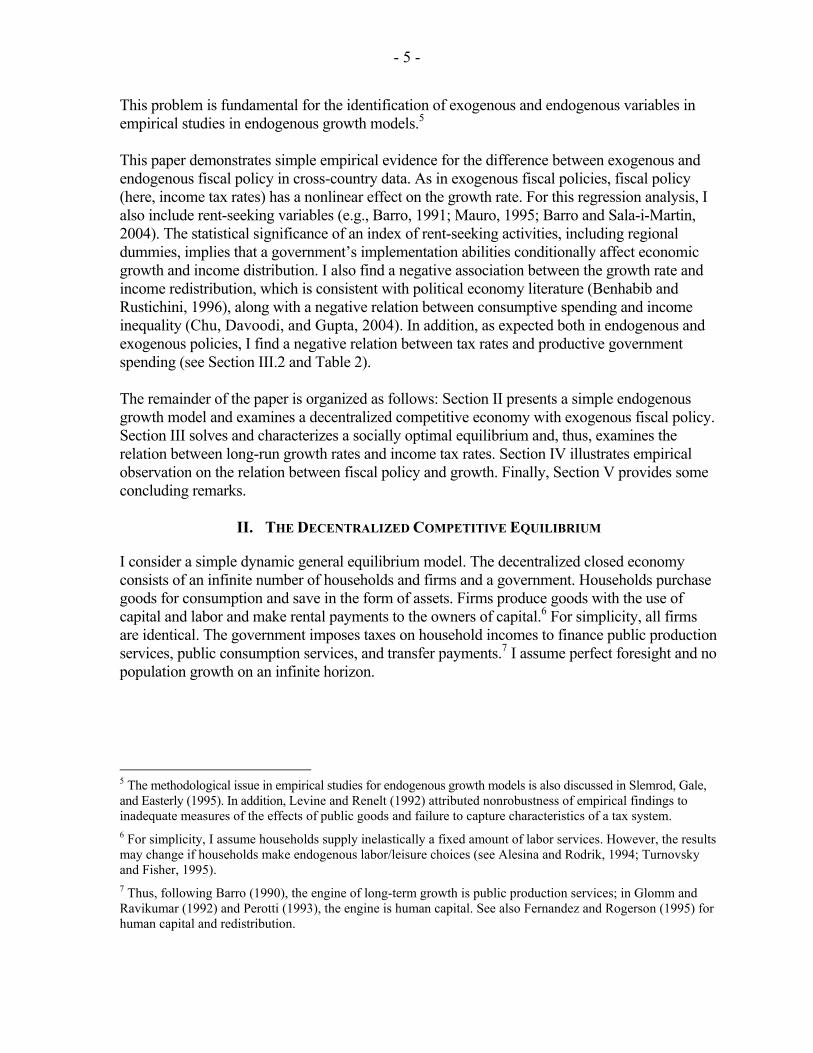
economy’s growth rate and the income tax rate is an inverse U-curve. At low tax rates (τ ′ in Figure 1), ατ −<< 10 , an increase in the tax rate increases growth. At high tax rates (τ ′′ in Figure 1), 11 <<− τα , the growth rate declines with the tax rate. The benchmark tax rate *τ is equal to α−1 . That is, this benchmark is related to the productivity of productive government expenditures and, thus, the spillover effect from public capital in the competitive economy. I also note that the nonlinearity is independent of the presence of consumptive expenditures, namely, public consumption and redistributive transfers.18 In other words, even though

0=γ or 0)( =iσ , the growth rate has the inverse U-curve in tax rates as long as the government provides the public capital (i.e., 0≠θ ), and the spillover effect is not zero (i.e.,

1,01 ≠−α ). The result is intuitive: With low tax rates, the positive effect of public production services on the productivity of private capital stocks exceeds the negative effect of distortionary tax on private capital accumulation. This situation leads to increased growth. With a high tax rate, the opposite occurs. Hence, the distortion of taxes increases nonlinearity and its efficiency loss swamps gain from public investment. This result is similar to that in endogenous growth models (e.g., Barro, 1990, 1991; Glomm and Ravikumar, 1992) and in political economy models (e.g., Alesina and Rodrik, 1994). In particular, Barro (1990, 1991) and Aschauer (1989) found a positive relation between productive spending and output growth, whereas output growth has a negative correlation with the share of consumptive government spending. Kneller, Bleaney, and Gemmell (1999) confirmed this relation with distortionary taxation for a panel of Organization for Economic Cooperation and Development (OECD) countries.

17 However, not all endogenous growth models predict the same positive effect of fiscal policy on growth; for example, Jones (1995) found that the long-run growth rate depends only on the exogenous population growth. 18 Giavazzi, Jappelli, and Pagano (2000), Mueller (2003, pp. 546), Peden (1991), and Hansson and Henrekson (1994), among others, discuss other sources of nonlinearity.

- 11 -

Figure 1. Growth Rates and Exogenous Fiscal Policy

),( θτφ

),(~

θτφ

0 τ ′ α−1 τ ′′ 1 τ~

However, the statistical relation between growth rates and almost every fiscal policy instrument including productive spending is not as robust (see Levine and Renelt, 1992; Easterly and Rebelo, 1993; Mendoza, Milesi-Ferretti, and Asea, 1997). The nonlinearity between expenditure policy and economic growth may be a source of statistical insignificance for cross-country analyses of the relation between various taxes and productive government expenditure. In other words, the nonlinear relation between fiscal policy and growth induces the nonlinearity between redistributive expenditure and economic growth. A few alternative views exist on the source of this nonrobustness. For example, Mendoza, Milesi-Ferretti, and Asea (1997) attribute ineffectiveness of tax policy in a long-run equilibrium to the mix of taxes, which has a negligible effect on growth of labor supply and savings. Alesina (1999) and Devarajan, Swaroop, and Zou (1996) believe that this empirical insignificance is because developing countries misallocate government expenditure in favor of productive spending at the expense of consumptive spending, whereas developed countries do the reverse. More important, when a fiscal variable is not strictly exogenous, empirical evidence based on cross-section or static-penal approaches may be misleading. In the next section I explore this possibility by optimally choosing some policy variables to be endogenous.

Gro

wth

Rat

e

Tax Rate

- 12 -

III. RAMSEY OPTIMAL POLICY AND EQUILIBRIUM

I now endogenize economic policy, τ and θ . I postulate that the government chooses a socially optimal Ramsey economic policy.19 Specifically, I solve for optimal policy under a benevolent government in a competitive economy, which is a second-best Ramsey problem. The Ramsey problem captures the incentive compatibility of individual agents, which internalizes externalities from public capital spillover and public consumption. As opposed to a socially efficient Pareto allocation, this problem enriches analysis for policy implementation. It can be based on asymmetric information between a policymaker and individual agents in the economy, and it is also consistent with a weak institution and rent-seeking behavior in the economy.20 That is, the benevolent government sets optimal policies subject to individual agents’ optimal decision rules in a decentralized competitive economy. Therefore, the government’s objective function is the sum of each household’s lifetime utility

[ ][ ]dtdiHicI

∫ ∫∞

+0 0

log)(log γ ,

and the government’s constraints are the incentive compatibility conditions (i.e. (1.1)), and the individual’s budget conditions (i.e. (1.2)).21 I show that endogenous optimal fiscal policies have different implications for economic growth than those of the exogenous policies previously discussed. This finding is supported by empirical studies including Levine and Renelt (1992) and Devarajan, Swaroop, and Zou (1996). Generally speaking, to understand performance in statistical tests for the relation between dependent (growth rates) and independent variables (fiscal policy instruments), I specify an alternative set of exogenous and endogenous variables by endogenizing τ and θ . Here, I characterize a Ramsey equilibrium under the set of endogenous policy variables τ and θ .22 This exercise illustrates the endogeneity problem in empirical studies on government policy for economic growth (e.g., Bleaney, Gemmell, and Kneller, 2001; Eicher and Garcia-Penalosa, 2001). Formally, the set of necessary conditions in (2.1) through (2.6) for socially optimal Ramsey policies in a dynamic competitive economy is summarized as follows (for details, refer to Appendix II):

19 Economic policy can be chosen by, for example, selfish voters, altruistic voters, a benevolent government, and so on (see Mueller, 2003, chapters 18, 22). 20 This dilemma is generally labeled the theory of rent seeking—referring to socially costly pursuit of income and wealth transfer. This alternative form of redistribution is to abstract, e.g., tax and expenditure from the specific policy mechanism (Mueller, 2003, chapter 15). 21 For technical details, please refer to Park and Philippopoulos (2003), who use a version closest to the present model. 22 For example, unlike my model of distortionary taxation, Easterly and Rebelo (1993) assumed that government revenue and expenditure are financed by lump-sum taxes and subsidies, which are likely to underestimate tax distortion in fiscal polices.

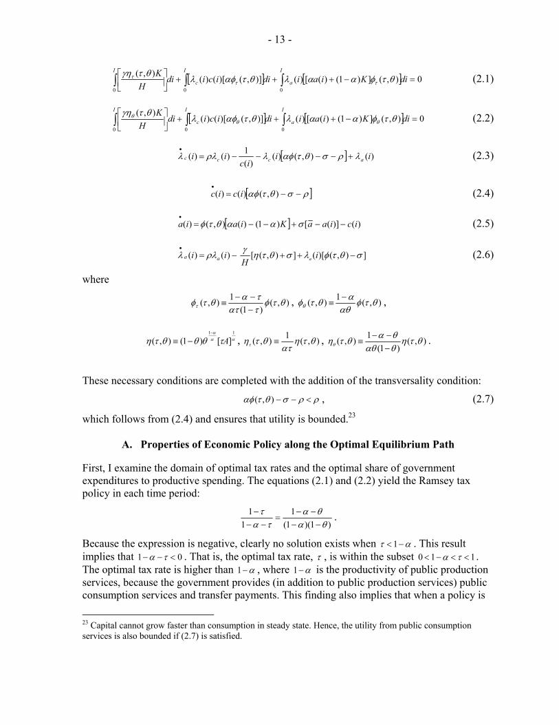
- 13 -

[ ] [ ] 0),(])1()([)()],()[()(),(

000

=−+++⎥⎦

⎤⎢⎣

⎡∫∫∫ diKiaidiicidi

HK I

a

I

c

I

θτφααλθταφλθτγη

τττ (2.1)

[ ] [ ] 0),(])1()([)()],()[()(),(

000

=−+++⎥⎦

⎤⎢⎣

⎡∫∫∫ diKiaidiicidi

HK I

a

I

c

I

θτφααλθταφλθτγη

θθθ (2.2)

[ ] )(),()()(

1)()( iiic

ii accc λρσθταφλρλλ +−−−−=•

(2.3)

[ ]ρσθταφ −−=•

),()()( icic (2.4)

[ ] )()]([)1()(),()( iciaaKiaia −−+−−=•

σααθτφ (2.5)

−=•

)()( ii aa ρλλ ]),()[(]),([ σθτφλσθτηγ−++ i

H a (2.6)

where

),()1(

1),( θτφτατταθτφτ −

−−≡ , ),(1),( θτφ

αθαθτφθ

−≡ ,

ααα

τθθθτη11

][)1(),( A−

−≡ , ),(1),( θτηατ

θτητ ≡ , ),()1(

1),( θτηθαθθαθτηθ −

−−≡ .

These necessary conditions are completed with the addition of the transversality condition:

ρρσθταφ <−−),( , (2.7)

which follows from (2.4) and ensures that utility is bounded.23

A. Properties of Economic Policy along the Optimal Equilibrium Path

First, I examine the domain of optimal tax rates and the optimal share of government expenditures to productive spending. The equations (2.1) and (2.2) yield the Ramsey tax policy in each time period:

)1)(1(1

11

θαθα

τατ

−−−−

=−−

− .

Because the expression is negative, clearly no solution exists when ατ −<1 . This result implies that 01 <−− τα . That is, the optimal tax rate, τ , is within the subset 110 <<−< τα . The optimal tax rate is higher than α−1 , where α−1 is the productivity of public production services, because the government provides (in addition to public production services) public consumption services and transfer payments. This finding also implies that when a policy is

23 Capital cannot grow faster than consumption in steady state. Hence, the utility from public consumption services is also bounded if (2.7) is satisfied.

- 14 -

optimally chosen, the result must be on the downward-sloping part of the growth rate–tax rate relation (see Devarajan, Swaroop, and Zou 1996; Hansson and Henrekson, 1994). Similarly, I also conclude that (2.2) implies 0)1( <−− θα . That is, for the same reason as previously outlined for τ , the optimal share of total tax revenues used to finance public production services, θ , is within the subset 110 <<−< θα . This property for endogenous variables provides an interesting comparison with the case in which policy variables are exogenous, as discussed in the previous section. This result is intuitive: Tax policy cannot be optimal when a higher tax rate can increase growth (which happens when ατ −<< 10 ). The spillover effect of public capital α−1 determines the range of optimal rate of taxes and optimal share of productive expenditures. Thus, the Ramsey tax rate should be higher than the socially efficient rate of tax ατ −=1 , which is the case in Barro (1990), for growth models with productive government spending. Moreover, as long as the government can choose its policy optimally, the nonlinear, inverse-U relation between the growth and tax rate disappears (see Figure 1). Hansson and Henrekson (1994) provide empirical evidence supporting this proposition.24 Therefore, the relation between fiscal policy (i.e., tax rates) and growth rates is qualitatively different depending on whether fiscal policy is endogenous or exogenous. Second, the previously discussed atemporal condition implies that the two policy instruments, τ and θ , move in opposite directions in each time period. That is, 0<∂∂ θτ . Intuitively, when the government allocates a larger share of tax revenues to public production services (i.e., θ increases), it can afford a lower tax rate (i.e., τ decreases) because public production services stimulate private investment and, hence, increase the tax base and tax revenues. That is, τ and θ are substitutes along the optimal path. This finding implies that room for fiscal consolidation exists. Although theoretically clear, colinearity is possible between tax rates and the share of productive expenditure, thus making the empirical evidence fragile. It may also lead to the lack of robustness for fiscal policy analysis on the composition of policy instruments, for example, various tax rates and variables of government expenditure (e.g., Easterly and Rebelo, 1993; Devarajan, Swaroop, and Zou 1996). Clearly in practice, τ and θ are hardly exogenous; thus, empirical evidence based on cross-country regressions can be biased.25 This point is illustrated empirically in Table 2, Section IV. Third, for given aggregate values of consumption, capital, and their shadow prices, total differentiation of (2.1) implies that the tax rate, τ , increases with )(iaa − . Thus, individuals/voters with capital endowments below (above) the average capital stock prefer high (low) tax rates. In other words, those with relatively little capital endowment prefer higher redistribution: If the median individual/voter is less endowed than the average, then

24 Hansson and Henrekson (1994) found that the government sector in none of the 14 OECD countries is smaller than a social equilibrium size for the period from 1965 to 1982 and from 1970 to 1987. 25 See Bleaney, Gemmell, Kneller (2001) for a method to deal with an endogeneity problem in a growth model with fiscal policy. Also see Alesina and Perotti (1995) and Gupta and others (2002).

- 15 -

the voting majority leads to higher taxes. Because the growth rate is negatively affected by the tax rate along the optimal path, it follows that initial inequality hurts growth. Persson and Tabellini (1994), Alesina and Rodrik (1994), and Benabou (1996) reached similar conclusions. However, my model is more general because the government provides explicit redistributive transfers as well as public (production and consumption) services. In addition, I also incorporate implementation conditions for the competitive economy in which the private agents are allowed to react to government policies.

B. A Special Case with No Consumptive Expenditure

I examine a special case in which no direct welfare gain results from consumptive spending. In other words, consumptive expenditure does not matter for the optimal consumption rate, and public consumption services do not offer any utility. Formally, 0=γ implies that (2.1) requires either 0=+ ac ac λλ , or 0),( =θτφ or 0)1( =−− τα . The first possibility (i.e.,

0)( =+ ac ac λλ ) cannot occur because it contradicts the dynamics implied by (2.3) through (2.6), and the second possibility, (i.e., 0),( =θτφ ) cannot occur whenever the economy grows. Therefore, the only possibility remaining is that the economy will not grow when 0=γ . This case is consistent with the following argument on Wager’s law. A third possibility for 0=γ is that 0)1( =−− τα (i.e., ατ −=1 ) in each time period, which is the socially optimal tax rate of Barro (1990) and Barro and Sala-i-Martin (1992, 2004). In other words, when 0=γ , the optimal tax rate is constant over time and equals the productivity of public services, α−1 , all the time. In turn, when 0=γ and ατ −=1 , the Ramsey tax policy equation implies 1=θ in all time periods; that is, when public consumption services offer no utility, using all tax revenues to finance public production services only is optimal. Note that a constant τ and a constant θ imply a constant return to capital, ),( θτφ . Then, (2.4) implies that the economy has no transitional growth dynamics. Therefore, when 0=γ , the necessary conditions for optimality imply that the economy adjusts immediately to its steady state and balanced growth path (see Barro, 1990; Barro and Sala-i-Martin, 1992; Alesina and Rodrik, 1994). In other words, the presence of nonproductive government expenditures opens the door for transitional dynamics. Hence, Fisher’s constant rule policy is no longer optimal. Furthermore, when 0=γ and government expenditures are not productive for firms (i.e.,

01 =−α ), then 0=τ in all time periods; that is, the Ramsey tax rate is zero all the time (see Chamley, 1986; Judd, 1985). This finding implies zero tax revenues and zero transfer payments. It also implies ),( θτφ , which excludes endogenous persistent growth (see (2.4)). Therefore, the government finds it optimal to redistribute income from the rich to the poor only when it also provides public (production and consumption) services, whereby public production services generate endogenous growth. This finding implies Wager’s law, in which government spending is complementary to economic growth and, thereby, per capita income growth.

- 16 -

C. Symmetric Long-Run Equilibrium

For the following discussion, it is useful to consider the special case in which all individuals are alike ex post at equilibrium. This symmetric Ramsey equilibrium26 coincides with the decision that is optimal for each individual with representative wealth and income. In other words, this special case is a representative agent economy. Apparently, in a symmetric equilibrium, all individuals own ex post the same amount of capital; thus, no actual transfers take place in equilibrium. This situation is not very restrictive. I have already shown how inequality affects policy and growth along the optimal path. The critical feature of redistribution is the expectation of transfers of income as opposed to actual transfers of income (see Benabou, 1996).27 Therefore, I invoke the symmetry conditions aia ≡)( , cic ≡)( , cc i λλ ≡)( , and aa i λλ ≡)( into the optimality conditions (2.1) through (2.6). By the usual transformations Kcz ≡ and aaλψ ≡ , the dynamics of (2.1) through (2.6) are equivalent to the dynamics of (A.1) through (A.4) in Appendix III, which constitute a four-equation dynamic system in ψθτ ,,,z . This transformation reduces the dynamic dimensionality of the model and facilitates analytical tractability. The remainder of this section studies the steady-state symmetric equilibrium in (A.1) through (A.4). That is, I focus on a long-run equilibrium in which all individuals own ex post the same amount of capital. This choice of a steady state follows naturally from the assumption that all individuals have the same rate of time preference. By contrast, heterogeneous rates of time preference would lead to a long-run equilibrium in which only patient agents hold capital.28 I now characterize a long-run symmetric Ramsey equilibrium in which the economy grows at a constant positive rate (i.e., balanced growth path; BGP), and economic policy does not change. Specifically, I solve for the following long-run equilibrium: (i) Consumption c , capital k , and asset a , grow at the same constant positive rate, which implies kcz ≡ is a

constant or 0=•z in (A.1); (ii) the policy instruments do not change; therefore, 0==

••θτ in

(A.2) and (A.3); and (iii) the social value of the economy’s capital stock (i.e., kaλψ ≡ ) in

26 Symmetric equilibria are not only interesting in themselves, but they can also provide insight into the properties of nonsymmetric equilibria, which are more complicated algebraically (see following discussion). This methodology is commonly used (e.g., Persson and Tabellini, 1992). On the other hand, see Fernandez and Rogerson (1995) and Greenwood and Jovanovic (1990) for ex post heterogeneity. 27 Benabou (1996) argued that the fight over the pie does not necessarily lead to higher transfers, just to higher distortions. 28 See also Bewley (1982). If endogenous discount rates are used, they become identical to all agents in the long run, and thereby agents own the same amount of capital (see Epstein, 1987).

- 17 -

(A.4) grows at a constant negative rate.29 That is, •ψ is negative.30 Appendix IV solves for the

long-run levels of z , τ , θ as well as the long-run rate of ψ and demonstrates the existence of BGP. Two summary equations of the long-run equilibrium z~ , τ~ , θ~ , corresponding to long-run η~ , φ~ , are:

0~)1()~1(~

~~~)1()( =

−−

++−−−+−φατργησ

ηγσηαγα z (3.1)

)~1)(1()~1(

)~1()~1(

θαθα

τατ

−−−−

=−−

− . (3.2)

Moreover, if the parameter values satisfy 0)1()1(11

1 <−+−−+

− αα

αα

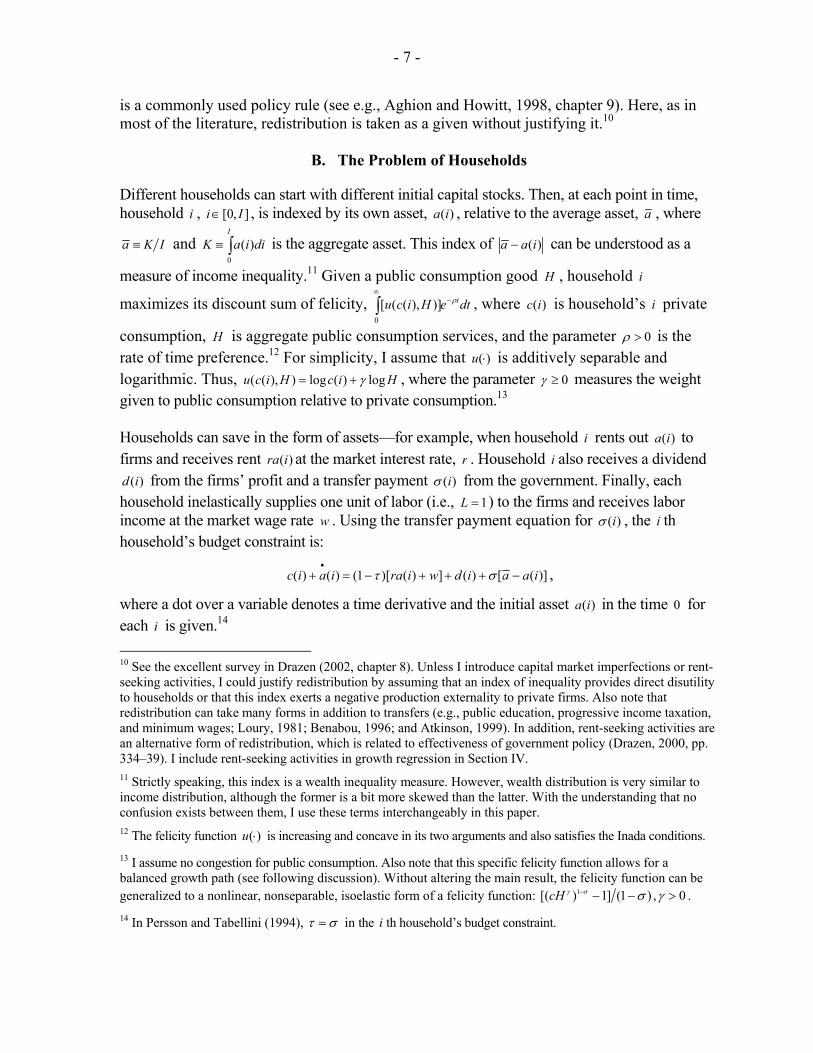
ααγγρ , the following exist: (i) a unique optimal long-run tax rate, τ~ , where 1~10 <<−< τα , and (ii) a unique optimal long-run allocation of tax revenues between productive and nonproductive government expenditures, θ~ , where 1~10 <<−< θα . Again, the benchmark is the productivity of public capital and the magnitude of spillover effect α−1 . Notice that the BGP tax rate and the BGP fraction of tax revenue to productive spending are located in the range in which the long-run growth rate decreases as the tax rates increase (see Figure 1). In turn, this policy supports a unique BGP along which long-run consumption and capital grow at the same unique positive constant rate. I illustrate the existence and uniqueness of BGP in Figure 2.

29 Equations (A.1) and (A.4) imply that if 0=

•z , then 0=

•ψ cannot be set. Instead, ψ should grow at a

constant negative rate (see following discussion). Technically, in the steady state, all variables are equal to a constant (zero is only one of many possible constant values).

30 The intuition behind a negative long-run •ψ is as follows. In standard models of long-term growth, the social

price of capital, aλ , decreases (i.e., 0<•

aλ ) when perpetual asset accumulation (i.e., 0>•a ) occurs;

specifically, it decreases at the same rate that capital increases, so that 0=•ψ . Here, because I also include

redistributive transfers, which require higher capital accumulation and larger tax bases to finance them, I need a stronger condition than usually; thus, aλ decreases at a higher rate than a increases.

- 18 -

Figure 2: Tax Rate and Share of Productive Spending with Endogenous Fiscal Policy

θ~

1

Equation (4.1)

α−1 Equation (4.2)

0 α−1 1 τ~

Tax Rate

The uniqueness of BGP helps characterize the property of fiscal policy. However, we also need to know the stability property of BGP for completing dynamic comparative analysis. The existence of multiple of BGPs is well-reported in endogenous growth models with the presence of externalities (Benhabib and Perli, 1994; Benhabib and Farmer, 1994; Park and Philippopoulos, 2003). In the following discussion, I examine evidence of multiplicity of optimal paths.

IV. EMPIRICAL OBSERVATIONS

In this section, I empirically test the complex relation between government fiscal policy and economic performance. As shown in the theoretical growth model, the growth rates and productive and consumptive policies are nonlinear; the statistical significance depends on the set of variables included in the regression analysis. These results suggest that nonlinearity and endogeneity must be taken into account when implementable policy instruments on economic growth are estimated. I show that the assumption in cross-country regressions of a common economic structure and the same fundamentals across countries can lead to incorrect statistical estimates. First, I test whether evidence exists of nonlinearity of exogenous fiscal policy affecting economic growth. Second, I investigate whether productive government spending is negatively associated with distortionary tax rates as predicted in Section III with endogenous policy. Third, I test for the negative association between economic growth and the redistributive policy and find no association between inequality and redistributive spending. Fourth, I find weak evidence of consumptive spending and income inequality. Finally, I investigate the possibility of existence of multiple equilibrium paths.

Shar

e of

Pro

duct

ion

Publ

ic S

pend

ing

- 19 -

I first investigate whether a nonlinear effect of exogenous fiscal policy on the growth rate exists.31 The idea of a nonlinear effect of fiscal policy on economic growth has been discussed often in the growth literature of the last 15 years. Suggestive evidence also exists that the effect of fiscal policy may vary across groups of countries. For example, Barro and Sala-i-Martin (2004, chapter 12) claimed that government consumption has a negative effect on growth for low-income countries, whereas its effect on high-income countries is insignificant.32 Table 1 presents another instance in which the effect of a fiscal variable (here, average tax rates or tax revenue over GDP) is nonlinear and different among groups of countries. Following Barro (1991), I regress the growth rate of each country i (growth) on a measure of average tax rates (tax) and a number of control variables. Following common practice in the empirical growth literature,33 the control variables include the log of the country’s initial level of per capita income (LGDP) to control for convergence effects, its degree of openness (openness), the investment share in GDP (investment share), an index of rent-seeking activities or the rule of law (ICRG), and three regional dummies for those countries located in East Asia, the sub-Saharan Africa, and Latin America (East Asia, sub-Saharan Africa, and Latin America, respectively). Data are collected data for 93 industrial and developing countries between 1990 and 2000. All variables are averaged over the 1990s, except, of course, for LGDP, which is the beginning of period value. The data for many of the variables come from the Penn World Tables, version 6.1 (Heston, Summers, and Aten, 2002). Specifically, I use the GDP per capita in constant prices to obtain the 10-year average of annual growth rates (growth) and the log of the initial level of GDP of 1990 to get LGDP in each country. Also, I use the sum of imports and exports over GDP (all in constant prices) to obtain a measure of openness. Finally, the share of investment in GDP is used for investment share. Both these variables are averaged over the 1990s. To obtain a proxy for private rent-seeking incentives or for the protection of property rights, I use the IRIS data set (version IRIS-3),34 This data set contains annual values for indicators of the violation of property rights, corruption, and quality of governance for the period from 1982 to 1997, as constructed by Stephen Knack and the IRIS Center, the University of Maryland, from monthly International Country Risk Guide data provided by Political Risk Services. This data set has been used in a series of related papers (see, among many others,

31 When fiscal policy is chosen optimally, no proposition exists because deviations always decrease welfare by definition. 32 Also see Levine and Renelt (1992), Tanzi and Zee (1997), and de Mello and Tiongson (2003). 33 For example, see Barro and Sala-i-Martin (2004, chapter 12). Different studies in the literature have obviously included several other variables in growth regressions as well. However, adding more variables would restrict the sample too much for what I want to accomplish in this paper, so I keep only the most commonly used variables. 34 IRIS data set information is obtained from http://www.countrydata.com.

- 20 -

Knack and Keefer, 1995; Barro, 1997; Barro and Sala-i-Martin, 2004).35 Note that higher scores denote better outcomes. To obtain a measure of the tax rate, I use two definitions: (i) tax revenue over GDP and (ii) tax revenue minus tax income from international trade, again over GDP. The difference between two definitions intends to capture the effects of tax distortion from foreign economies. This dual definition can justify the openness variable (openness) in regression. Both variables can be obtained from the World Development Indicators CD-ROM and are averaged over the 1990s. The first variable is used in columns (1) to (4) in Table 1, and the second, in column (5).

35 Five subjective indices are available from the IRIS data set: corruption in government, rule of law, risk of repudiation of government contracts, risk of expropriation, and quality of bureaucracy. I follow the literature in obtaining an aggregate measure for productive versus unproductive activities by summing these five different indices, with higher scores indicating better social behavior observed. Note that from these indices, corruption in government, rule of law, and quality of bureaucracy range in value from zero to 6, whereas risk of repudiation of government contracts and risk of expropriation are scaled from zero to 10 with higher values indicating better ratings (i.e., less corruption and less risk). The aggregate measure of rent seeking is then constructed from these variables on a 50-point scale by converting corruption in government, rule of law, and quality of bureaucracy to a 10-point scale and summing them up with the other two indices.

- 21 -

Table 1. Growth Regressions: A Nonlinear Effect of Tax Revenues on the Growth Rate

Notes: LGDP = the country’s initial level of per capita income. ICRG = the rule of law. Ordinary least squares regressions t-ratios are in parentheses. The tax variable in columns (1) to (4) is the tax revenue over gross domestic product (GDP). Column (5) shows the tax revenue minus taxes on international trade over GDP. * indicates significance at the 10 percent level. ** indicates significance at the 5 percent level. I consider a linear-in-parameters model of the form of iii uXbagrowth ++= * , where a is a constant, b is the parameter vector, iX consists of the explanatory variables, and iu is the error term, where ),0(~ 2σNui . I capture the nonlinear relations between the growth rate and the tax rate by introducing the square of the tax rate as a variable in iX . The rest of the control variables included in iX are those previously described. Table 1 presents ordinary least squares regression estimates of the parameters and the t-statistic for each estimated coefficient to test its statistical significance. This specification of variables is roughly reduced from the previously described theoretical equations with the set of either endogenous or exogenous policy variables. For example, tax represents the income tax rate τ in the previous sections,36 and (tax)2 captures the nonlinearity of effects of fiscal policy on economic growth. LGDP shows the initial income differences, and investment share indicates private investment and capital accumulation. Also ICRG and a regional dummy are

36 Because τ is monotonically related with θ (see equation ),( θτφ in Section 2 and (2.6)), I must choose one variable (here τ ) for estimation.

Dependent variable:

Growth rate All

countries Low and middle

income All countriesLow and middle

income Low and middle

income (1) (2) (3) (4) (5)

Tax –0.0465

(–1.10) –0.0793

(-1.20) 0.0008

(0.01) 0.2851

(1.43) 0.0981

(0.58)

(Tax)2 — — –0.001

(–0.39) –0.0093*

(–1.93) –0.0067

(–1.45)

LGDP –1.3185**

(–2.31) –0.8285

(–1.23) –1.3456**

(–2.33) –0.8735

(–1.33) –0.6641

(–1.02)

Investment share 0.0767

(1.35) 0.0788

(1.10) 0.0789

(1.37) 0.0918

(1.31) 0.0817

(1.19)

Openness 0.0035

(0.59) –0.0171

(–1.46) 0.00352

(0.58) –0.0203*

(–1.77) –0.0199*

(–1.87)

ICRG 0.1657**

(2.47) 0.2257**

(2.50) 0.1649**

(2.45) 0.2220**

(2.51) 0.2525**

(2.93)

East Asia 0.6596

(0.68) 1.3389

(1.12) 0.6088

(0.62) 0.9577

(0.81) 0.8555

(0.73) Sub-Saharan

Africa –1.9101**

(–2.48) –1.3137

(–1.51) –1.9184**

(–2.48) –1.3956

(–1.64) –1.5061*

(–1.78)

Latin America 0.2888

(0.41) 0.0888

(0.11) 0.2524

(0.35) –0.3401

(–0.41) –0.3113

(–0.38)

Constant 6.8347**

(2.06) 2.7899

(0.64) 6.6134*

(1.96) 0.4646

(0.10) –0.0750

(–0.02) Adj. R2 (%) 24.24 26.15 23.46 29.53 31.29 Number of

observations 93 66 93 66 66

- 22 -

related with rent seeking and a rule of law and, thereby, policy implementation conditions in a competitive economy. Column (1) presents a standard growth regression, in which tax is not significant. The remainder of the control variables exerts their expected effect. However, only LGDP, ICRG, and sub-Saharan Africa are statistically significant. The significance of LGDP implies that conditional convergence is supported, whereas the positive and significant effect of the ICRG index is in accordance with the results of the rest of the relevant empirical literature (e.g., Knack and Keefer, 1996; Barro, 1997; Barro and Sala-i-Martin, 2004). This effect is noteworthy as it is very robust and remains highly significant in all the specifications reported in Table 1. This result suggests that the effective implementation of government policy is critical to economic growth. Weak institution and corruption can reduce the effectiveness of government policy. For instance, weakening the protection of property rights is found to be unfavorable for economic growth. This correlation between weak institution and policy effectiveness suggests that fiscal policy in developing countries may affect growth differently than in developed and developing countries. Column (2) reports the results from the same regression for a subsample of the initial data set, obtained by dropping high-income countries, which results in 66 remaining countries. This subsampling helps pin down whether structural differences exist across countries. However, the results are basically the same: tax is again insignificant. The remaining columns incorporate the nonlinearity in regression analysis. Column (3) presents for all the countries a nonlinear relation between economic growth and the tax rate—and does so without much support as the quadratic term is not significant. Column (4) is significant as it incorporates both types of possible nonlinear effects. First, I restrict the sample to the non-high-income countries. Second, I add the quadratic term. Here, the quadratic term is significant, and, also, the fit of the regression is overall much improved, as almost all t-ratios are higher under this specification. Thus, this nonlinear specification appears to best fit the data. I also show that the nonlinearity, if it exists, is more likely to be observed in low- and middle-income countries. As noted previously, a structural difference may exist between high-income countries and low- and middle-income countries. Among many other unobservable variables, the magnitude of spillover from public capital can contribute the structural differences across countries (Knack and Keefer, 1977). Differences in policy implementation capacity (e.g., enforcement, corruption, information, coordination, etc.) may also come into play. To test robustness, I repeat column (4) in column (5), replacing tax revenue over GDP with tax minus trade taxes over GDP as the proxy of tax rates. The results are quite similar, but the quadratic term is less significant. This result suggests that the definition of tax rates for previous regressions can be biased due to nonlinearity. The remainder of the empirical analysis is limited to OECD countries because data are lacking for other countries. They are not regression analyses because the variables examined can be either exogenous or endogenous, depending on the theoretical model previously

- 23 -

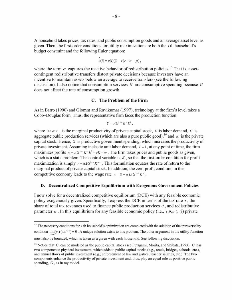
discussed. The main purpose of these exercises is not to claim a solid statistical relation but to find a simple association between variables of interest. First, I examine the relation between average tax revenue (equivalent here to the income tax rate) and productive government spending. As expected in the model with endogenous fiscal policy (see (3.2)), tax rates are negatively related with productive government spending both in the short and long run. Hence, when government spending is productive, the tax rate can be reduced in a socially optimal allocation (see Figure 3 and Table 2). More specifically, Theta is productive government spending over total government spending minus interest payments. The data on government spending are based on simple calculations, using data from the International Monetary Fund’s Government Financial Statistics (GFS) database; again, these data are general government spending. The classification into productive and unproductive spending is done following Bleaney, Gemmell, and Kneller (2001). In particular, productive government expenditure includes education, transport and communication, defense, housing, health, and general public services. The (effective) tax rate is the ratio of income tax revenue over GDP. These data are again obtained by using GFS, following the classification of Bleaney, Gemmell, and Kneller (2001). In particular, the data include the following taxes: income taxation, social security taxes, taxes on payroll, and taxes on property.

Figure 3. Tax Rate and the Fraction of Productive Government Spending

.3

.4

.5

.6

.7

Frac

tion

of P

rodu

ctiv

e G

over

nmen

t Spe

ndin

g

.05 .1 .15 .2 .25 .3 (Effective) Tax Rate

- 24 -

Table 2. Correlations between the (Effective) Tax Rate and the Fraction of Productive Government Spending (theta) for 26 OECD Countries

Distorting tax revenue (70–00)

Distorting tax revenue (80–00)

Distorting tax revenue (90–00)

Theta(70–00) –0.4745 Theta(80–00) –0.5241 Theta(90–00) –0.4782 Number of observations 26 26 23

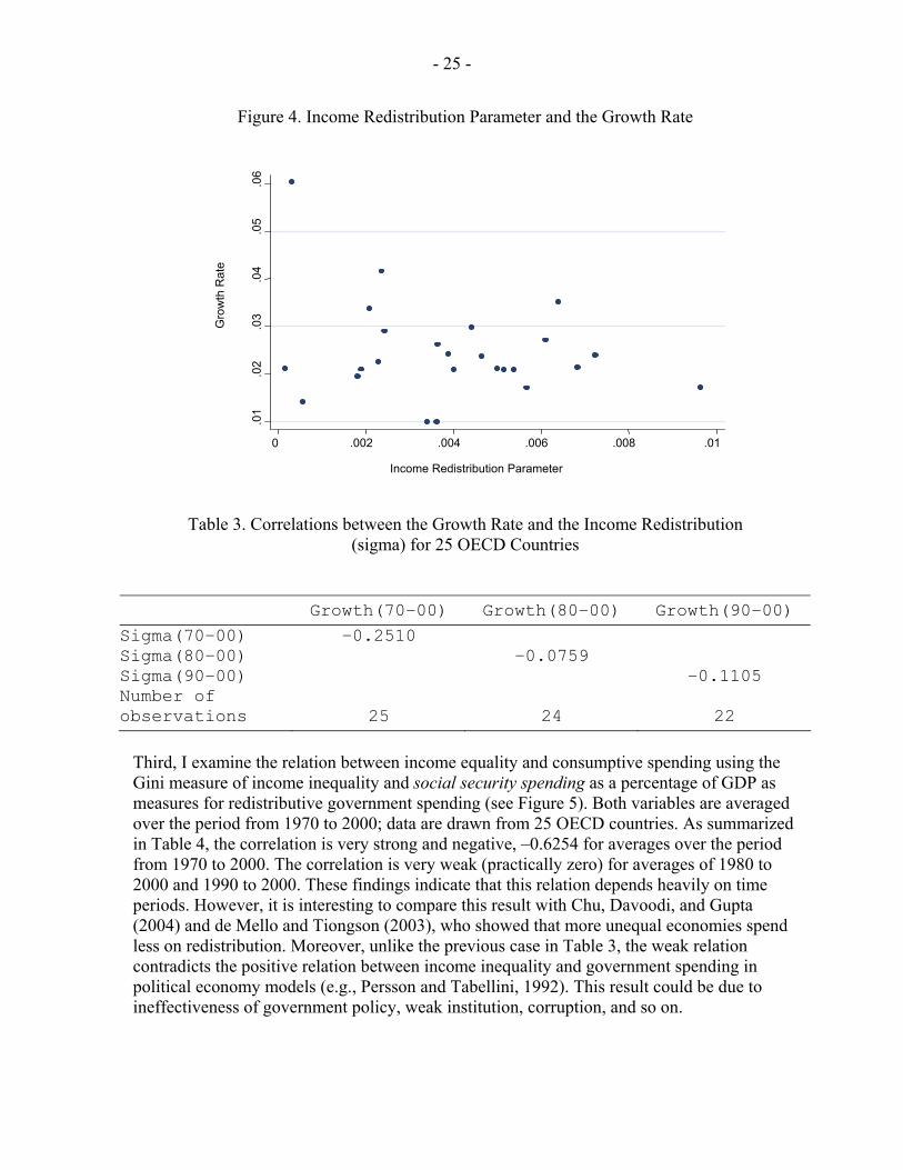
Second, I examine the correlation between economic growth and income distribution. Data on real growth rate are obtained using GDP in constant prices data from the Penn World Tables, version 6.1 (Heston, Summers, and Aten, 2002). For all cases, 70–00 indicates that the variable is averaged over the period from 1970 to 2000; 1980 to 2000 and 1990 to 2000 are interpreted similarly. Sigma, σ , is an income redistribution index defined as the share

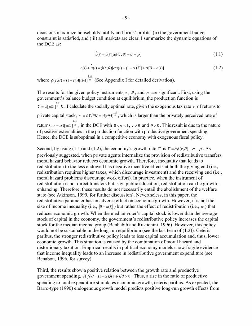
)(iσ of consumptive government spending in social security and welfare as a percentage of GDP over the Gini coefficient (i.e., a proxy for income difference, )(iaa − ) of income inequality, which is consistent with )]([)( iaai −=σσ as defined in Section II. Both variables are averaged over the indicated periods. The Gini index is obtained using the high-quality data set in Deininger and Squire (1996). Data on government spending on social security and welfare is obtained from the GFS database.37 The GFS database is also used for all data on government spending and taxation referred to in the following discussion. Figure 4 illustrates the correlation between growth rates and the index of income redistribution, and Table 3 summarizes their relation. As expected in the theoretical model with both exogenous and endogenous fiscal policy, the indices of income redistribution and economic growth have a negative association. This result is consistent with political economic models (see, e.g., Alesina and Rodrik, 1994), in which both variables are endogenous.

37 I am grateful to C. Wu and P. Kammas for providing the data.

- 25 -

Figure 4. Income Redistribution Parameter and the Growth Rate

Table 3. Correlations between the Growth Rate and the Income Redistribution (sigma) for 25 OECD Countries

Growth(70–00) Growth(80–00) Growth(90–00) Sigma(70–00) –0.2510 Sigma(80–00) –0.0759 Sigma(90–00) –0.1105 Number of observations 25 24 22

Third, I examine the relation between income equality and consumptive spending using the Gini measure of income inequality and social security spending as a percentage of GDP as measures for redistributive government spending (see Figure 5). Both variables are averaged over the period from 1970 to 2000; data are drawn from 25 OECD countries. As summarized in Table 4, the correlation is very strong and negative, –0.6254 for averages over the period from 1970 to 2000. The correlation is very weak (practically zero) for averages of 1980 to 2000 and 1990 to 2000. These findings indicate that this relation depends heavily on time periods. However, it is interesting to compare this result with Chu, Davoodi, and Gupta (2004) and de Mello and Tiongson (2003), who showed that more unequal economies spend less on redistribution. Moreover, unlike the previous case in Table 3, the weak relation contradicts the positive relation between income inequality and government spending in political economy models (e.g., Persson and Tabellini, 1992). This result could be due to ineffectiveness of government policy, weak institution, corruption, and so on.

.01

.02

.03

.04

.05

.06

Gro

wth

Rat

e

0 .002 .004 .006 .008 .01 Income Redistribution Parameter

- 26 -

Figure 5. Redistributive Government Spending and Income Inequality

Table 4. Correlations between Redistributive Government Spending (RGS) and Income Inequality (Gini) for 25 OECD Countries

Gini(70–00) Gini(80–00) Gini(90–00)

RGS(70–00) –0.6254 RGS(80–00) 0.1715 RGS(90–00) 0.1718 Number of observations 25 25 22

Finally, the last exercise examines whether a hint of multiple equilibrium paths exists around the BGP. Table 5 summarizes the relation between σ and GNP variance. I find that the relation is positive but weak: The more intensive the redistributive policy, the higher the variance of GDP (see Figure 6). This finding suggests that more than one equilibrium can exist around the BGP. In the context of this study, multiple equilibria can occur when income redistribution causes externalities, inefficiency, free riding, or moral hazard in a competitive economy (Benhabib and Farmer, 1994).

2030

40

50

60

Inco

me

Ineq

ualit

y (G

ini)

0 .1 .2 .3

Redistributive Government Spending

- 27 -

Figure 6. Income Redistribution Parameter and GDP Variance

Table 5. Correlations between the Income Redistribution (sigma) and the Variance of GDP for 25 OECD Countries

GDP variance

(70–00) GDP variance

(80–00) GDP variance

(90–00) Sigma(70–00) 0.2043 Sigma(80–00) 0.1930 Sigma(90–00) 0.1183 Number of observations 25 25 22

However, if the outliers (Luxembourg with a high variance, and Denmark with a high sigma) are excluded from the data set, the correlation is practically zero. Hence, this observation is less likely to support the argument that multiple equilibria exist. It must be emphasized, that these correlation results do not constitute empirical evidence. Nevertheless, strong correlations between tax rates and productive spending (see Table 2) suggest something about a relation between variables, which is useful information.

0

2.00

e+07

4.0

0e+0

7 6.

00e+

07 8

.00e

+07

GD

P v

aria

nce

0 .002 .004 .006 .008 .01

Income Redistribution Parameter

- 28 -

V. CONCLUDING REMARKS

Main conclusions of this study can be summarized as follows. First, in a general equilibrium model with given exogenous fiscal policy (i.e., income tax, share of government expenditure between consumptive and productive government spending, and redistributive government transfers), a nonlinear relation exists between the suboptimal long-run growth rate in the competitive economy and distortionary tax rates because government policy can have mixed results. On one hand, a government’s productive spending can have direct positive effects on the efficiency and growth of private economic sectors facilitating the transportation and legal system, enforcing the contracts, reducing social conflicts by reducing economic inequality and poverty, and so on. On the other hand, government activities can have negative effects on economic productivity by lowering work effort and savings with high taxation, diverting productive activity to rent-seeking activity, crowding out private activities, and so on. Second, when fiscal policy is endogenously chosen at a social optimum, the relation between the rate of growth and tax rates is always negative. That is, the endogenous optimality condition for fiscal policy eliminates the increasing proportion of the hump. Therefore, as long as the government has sufficient policy instruments and can effectively implement them for promoting growth and improving equity, this model predicts a negative relation between tax rates and growth rates in a competitive economy. These two conclusions suggest that the interaction among fiscal policies may be complicated enough that it cannot be captured in a simple linear model using aggregate measure of fiscal policies. The sources of nonlinearity include expectation and coordination of fiscal policies, impulse response of government policies, and the presence of positive externality due to government spending. In addition, this study shows that ambiguous empirical results of fiscal policy on growth can result from endogeneity of policy variables, and endogeneity induces the reverse causality of public investment and economic growth. Notably, Mankiw, Romer, and Weil (1992) and Barro and Sali-i-Martin (1992, 2004), along with many others, treat the investment rate as an exogenous growth determinant. By choosing a set of independent variables, the theoretical framework locates a source of sensitivity of empirical results, which thereby points toward a source of empirical endogeneity of fiscal policy and economic growth. The statistical significance can depend on which policy variables are included in the regression analysis, which suggests an estimation technique is needed that takes into account this endogeneity when estimating and interpreting empirical relations. This study also shows that the assumption in cross-country regressions of a common economic structure and the same fundamentals across countries can lead to incorrect statistical inferences.

- 29 - APPENDIX I

The Decentralized Competitive Equilibrium with Exogenous Policies

Given the government budget constraint =++ ∫1

0

)( diiHG σ ∫ +I

diwira0

])([τ and the three

components: )(,, iHG σ of government expenditure, =G ∫ +I

diwira0

])([τθ and

=+ ∫I

diiH0

)(σ ∫ +−I

diwira0

])([)1( τθ , the choice of τ , θ , and σ completely characterizes economic

policy because only two of the five policy instruments (e.g., ,,,, θτHG and σ ) can be independently set. Using the productive government spending G in the firm’s first order conditions, the return to

capital is αα

τθαθαφ−

=≡1

)(),( AAbr , which is the return that drives private agents’ consumption/saving decisions in a DCE. In the presence of productive government expenditure and thereby production externality, this return is smaller than the realized one (see the following

discussion). Moreover, the zero profit condition yields the wage rate KAAw αα

τθα−

−=1

)()1( . Using r , w into the previously stated government expenditure function and the production function, the economy-wide public production services, G , public consumption services, H ,

and output, Y , are, respectively: KAG ατθ1

][= ; ∫ −−−=− 1

0

11

)]([][)1( diiaaKAH στθθ ααα

; and

KAY αα

ατθ−

=1

][ ,38 where )(ia and thus ∫≡I

diiaK0

)( have been chosen by private agents who

ignored the effect of productive public spending. Therefore, I summarize the dynamics of the DCE as

]),()[()( ρσθταφ −−=•

icic (1.1)

)]([])1()()[,()()( iaaKiaiaic −+−+=+•

σααθτφ , (1.2)

where αα

τθτθτφ−

−≡1

][)1(),( AA .

38 The production function, KAY ααατθ )1(][ −= , shows that my model is a variant of the AK model of endogenous growth. That is, at economy-wide level, output is linear in capital (e.g., Barro, 1990; Barro and Sala-i-Martin, 2004, chapter 4).

- 30 - APPENDIX II

The Ramsey Optimal Equilibrium with Endogenous Policies

Recall the i th household’s budget constraints and Euler equations in combination with the rate of returns r and the wage rate w and the motion of the economy’s public goods, G and H in a DCE (see the DEC condition in Appendix I). The current-value Hamiltonian ( , , , , , )c ac a τ θ λ λℑ for the government is:

didiiaaKicacI I

ac ∫ ∫ ⎥⎦

⎤⎢⎣

⎡⎥⎦

⎤⎢⎣

⎡−−+≡ℑ

0 0

)]([),(log)(log),,,,,( σθτηγλλθτ

+ [ ]∫ −−I

c diici0

),()()( ρσθταφλ + [ ]diiciaaKiaiI

a∫ −−+−+0

)()]([])1()()[,()( σααθτφλ ,

where )(iaλ and )(icλ are the co-state variable associated with the i th household’s budget constraint and Euler equation, respectively. Then, the first-order conditions for

)(),(,,, iic ac λλθτ , and )(ia are (2.1) through (2.6), respectively.39

39 The utility function and the constraints are continuous and bounded, the utility function is strictly concave in the control variables θτ ,),(ic , and the constraints are linear in )(ic and strictly concave in τ and θ . Further, because the utility function and the constraints are both jointly concave in the control variables θτ ,),(ic and the state variable )(ia , the necessary conditions of (2.1) through (2.7) are also sufficient for optimality.

- 31 - APPENDIX III

The Symmetric Ramsey Equilibrium

If I impose the symmetry conditions, take the logarithms of (2.1) and (2.2), differentiate with respect to time, use (2.3), (2.4), (2.5), and (2.6) for the rates of growth of kcc ,,λ and aλ , and use the definition kaλψ ≡ , I get (A.2) and (A.3). Equation (A.1) follows easily if I differentiate kcz ≡ with respect to time and then use (2.4) and (2.5). Finally, (A.4) follows if I differentiate kaλψ ≡ with respect to time and then use (2.5), (2.6), and the definition kcz ≡ . Thus, the dynamics of a symmetric equilibrium are summarized as:

[ ]ρσθτφα −−−−=•

),()1(zz (A.1)

),,(),( ψθτθττ DB=•

(A.2)

),,(),( ψθτθτθ DE=•

(A.3)

⎥⎦

⎤⎢⎣

⎡+−−+=

•

),(1]ˆ[

θτησγψδρψ z , (A.4)

where 1

)1)(1()1)(1)(1(

)1()1()1(),(

−

⎥⎦

⎤⎢⎣

⎡−−−−−−−

−−−

−−−−≡

ταττθαθα

τααταααθτB ,

),()1()1()1()(),,(θτφα

τργσηηγσηαγαψθτ

−−

++−−−+−≡ zD ,

[ ] 1

)1)(1()1()1()1(1),(

−

⎥⎦

⎤⎢⎣

⎡−−−

−−−−−−

−−≡

θαθαττααατθ

ααθτE .

- 32 - APPENDIX IV

The Long-Run Ramsey Equilibrium To solve for the long-run levels of z , τ , and θ , as well as the long-run rate of ψ , I start with (3.1). Setting it equal to zero, I simply have 0~)1(~ >++−= ρσφαz (here, tildes above variables denote their long-run values), so that the long-run consumption-to-capital ratio, z~ , equals the discount factor, 0>ρ , plus the effective redistributive parameter, 0>σ . I continue with (A.2) and (A.3). For 0==

••θτ to hold, I must have 0)~,~,~( =ψθτD in (A.1)

through (A.4). Sufficient condition for 0)~,~,~( =ψθτD is:

0~)1()~1(~

~~~)1()( =

−−

++−−−+−φατργησ

ηγσηαγα z . (3.1)

From (A.4),

0~~1~ >⎥⎦

⎤⎢⎣

⎡+−+=

ψγ

ησσρz .

The atemporal condition for the Ramsey tax policy, which links the two policy instruments, τ and θ , must also hold in the long run. Thus, in steady state,

)~1)(1()~1(

)~1()~1(

θαθα

τατ

−−−−

=−−

− . (3.2)

Equations (3.1) and (3.2) can be solved for the long-run values τ~ , θ~ , and ψ~ . Notice that (3.1) and (3.2) constitute a two-equation system in τ~ and θ~ only. Therefore, the main task is to solve (3.1) and (3.2) for τ~ and θ~ . Now, (3.1) and (3.2) imply that 1~10 <<−< τα and 1~10 <<−< θα . Total differentiation of

(3.1) implies 0)~1)(1(~

]~)~1)(1[(~

~

~<

−−−−−−−−

=∂∂

τααττατααθ

τθ , and total differentiation of (3.2) implies

0~~~~<−=∂∂ τθτθ . Hence, (3.1) and (3.2) have a negative slope, and (3.1) is always steeper

than (3.2). Therefore, if (3.1) and (3.2) intersect, then they can intersect only once. To check whether they intersect, I examine two boundary conditions for )1( α− and 1. First, as )1(~ ατ −→ , (3.2) implies 1~

→θ , whereas as 1~ →τ , this equation implies αθ −→1~ . Second, because (3.1) is always steeper than (3.2), for (3.1) and (3.2) to intersect, when αθ −→1~ , (3.1) must imply a value of τ~ less than 1. More specifically, when αθ −→1~ and

0)1()1(11

1 <−+−−+

− αα

αα

ααγγρ , 1~ →τ cannot be a solution to (3.1). Therefore, a unique intersection point exists, which is illustrated in Figure 2.

- 33 -

References Aghion, Philippe, and Peter Howitt, 1998, Endogenous Growth Theory (Cambridge,

Massachusetts: MIT Press). Alesina, Alberto, 1999, “Too Large or Too Small Governments,” in Economic Policy and

Equity, ed. by V. Tanzi, K. Chu, and S. Gupta (Washington: International Monetary Fund), pp. 216–49.

Alesina, Alberto, Silvia Ardagna, Roberto Perotti, and Fabio Schiantarelli, 2002, “Fiscal

Policy, Profits, and Investment,” American Economic Review, Vol. 92, No. 3, pp. 571–89.

Alesina, Alberto, and Roberto Perotti, 1995, “Fiscal Expansion and Fiscal Adjustments in

OECD Countries,” Economic Policy, Vol. 21, pp. 205–48. ––––––, 1997, “Fiscal Adjustment of OECD Countries: Composition and Macroeconomic

Effects,” Staff Papers, International Monetary Fund, Vol. 44 (June), pp. 210–48. Alesina, Alberto, and Dani Rodrik, 1994, “Distributive Politics and Economic Growth,”

Quarterly Journal of Economics, Vol. 109, pp. 465–90. Aschauer David, 1989, “Is Public Expenditure Productive?” Journal of Monetary Economics,

Vol. 23, No. 2, pp. 177–200. Atkinson, Anthony, 1999, The Economic Consequences of Rolling Back the Welfare State

(Cambridge, Massachusetts: MIT Press). Barro, Robert J., 1990, “Government Spending in a Simple Model of Endogenous Growth,”

Journal of Political Economy, Vol. 98, No. 5, pp. S103–25. ––––––, 1991, “Economic Growth in a Cross Section of Countries,” Quarterly Journal of

Economics, Vol. 106 (May), pp. 407–43. ––––––, 1997, Determinants of Economic Growth: A Cross-Country Empirical Study

(Cambridge: Massachusetts: MIT Press). Barro, Robert, and Xavier Sala-i-Martin, 1992, “Public Finance in Models of Economic

Growth,” Review of Economic Studies, Vol. 99, No. 4, pp. 645–61. ––––––, 2004, Economic Growth, 2nd edition (Cambridge, Massachusetts: MIT Press). Benabou, Roland, 1996, “Inequality and Growth,” NBER Macroeconomics Annual, Vol. 11,

pp. 11–74.

- 34 -

––––––, 2000, “Unequal Societies: Income Distribution and Social Contract,” American Economic Review, Vol. 90, No. 1, pp. 96–129.

Benhabib, Jess, and Roger Farmer, 1994, “Indeterminacy and Increasing Returns,” Journal of

Economic Theory, Vol. 63, No. 1, pp. 19–41. Benhabib, Jess, and Robert Perli, 1994, “Uniqueness and Indeterminacy: On the Dynamics of

Endogenous Growth,” Journal of Economic Theory, Vol. 63, No. 1, pp. 113–42. Benhabib, Jess, and Aldo Rustichini, 1996, “Social Conflict and Growth,” Journal of

Economic Growth, Vol. 1, No. 1, pp. 125–42. Bewley, Truman, 1982, “An Integration of Equilibrium Theory and Turnpike Theory,”

Journal of Mathematical Economics, Vol. 10, pp. 284–306. Bleaney, Michael, Norman Gemmell, and Richard Kneller, 2001, “Testing the Endogenous

Growth Model: Public Expenditure, Taxation, and Growth over the Long Run,” Canadian Journal of Economics, Vol. 34, pp. 36–57.

Bourguignon, Francois and Christian Morrisson, 1998, “Income Equality and Development,”

Journal of Development Economics, Vol. 57, pp. 233–57. Buchanan, James M., and Richard E. Wagner, 1977, Democracy in Deficit: The Political

Legacy of Lord Keynes (New York: Academic Press). Chamley, Christophe, 1986, “Optimal Taxation of Capital Income in General Equilibrium

with Infinite Lives,” Econometrica, Vol. 54, No. 3, pp. 607–22. Chu, Ke-Young, Hamid Davoodi, and Sanjeev Gupta, 2004, “Income Distribution and Tax

and Government Social-Spending Policies in Developing Countries,” in Inequality, Growth, and Poverty in an Era of Liberalization and Globalization, ed. by G. Cornia (New York: Oxford University Press).

Cooley, Thomas, and Stephen LeRoy, 1981, “Identification and Estimation of Money

Demand,” American Economic Review, Vol. 71, No. 5, pp. 825–44. Deininger, Klaus, and Lyn Squire, 1996, “A New Data Set Measuring Income Inequality,”

The World Bank Economic Review, Vol. 10, No. 3, pp. 565–91. de Mello, Luiz, and Erwin Tiongson, 2003, “Income Inequality and Redistributive

Government Spending,” IMF Working Paper 03/14 (Washington: International Monetary Fund). Available via the Internet: http://www.imf.org/external/pubs/ft/wp/2003/wp0314.pdf

- 35 -

Devarajan, Shantayanan, Vinaya Swaroop, and Heng-Fu Zou, 1996, “The Composition of Public Expenditure and Economic Growth,” Journal of Monetary Economics, Vol. 37, No. 2–3, pp. 313–44.

Drazen, Allan, 2000, Political Economy in Macroeconomics (Princeton, New Jersey:

Princeton University Press). Easterly, William, and Sergio Rebelo, 1993, “Fiscal Policy and Economic Growth: An

Empirical Investment,” Journal of Monetary Economics, Vol. 32, No. 3, pp. 417–58. Eicher, Theo S., and Cecilia Garcia-Penalosa, 2001, “Inequality and Growth: The Dual Role

of Human Capital in Development,” Journal of Development Economics, Vol. 66, pp. 173–97.

Epstein, Larry, 1987, “The Global Stability of Efficient Intertemporal Allocations,”

Econometrica, Vol. 55, No. 2, pp. 329–55. Fernandez, Raquel, and Richard Rogerson, 1995, “On the Political Economy of Education

Subsidies,” Review of Economic Studies, Vol. 62, No. 2, pp. 249–62. Forbes, Kristin, 2000, “A Reassessment of the Relationship Between Inequality and

Growth,” American Economic Review, Vol. 90, No. 4, pp. 869–87. Futagami, Koichi, Yuichi Morita, and Akihisa Shibata, 1993, “Dynamic Analysis of an

Endogenous Growth Model with Public Capital,” Scandinavian Journal of Economics, Vol. 95, No. 4, pp. 607–25.

Galor, Oded, and Daniel Tsiddon, 1997, “Technological Progress, Mobility, and Economic

Growth,” American Economic Review, Vol. 87, No. 3, pp. 363–82. Giavazzi, Francesco, Tullio Jappelli, and Marco Pagano, 2000, “Searching for Non-Linear

Effects of Fiscal Policy: Evidence from Industrial and Developing Countries,” European Economic Review, Vol. 44, No. 7, pp. 1259–89.

Glomm, Gerhard, and B. Ravikumar, 1992, “Public versus Private Investment in Human

Capital: Endogenous Growth and Income Inequality,” Journal of Political Economy, Vol. 100, No. 4, pp. 813–34.

––––––, 1997, “Productive Government Expenditures and Long-Run Growth,” Journal of

Economic Dynamics and Control, Vol. 21, No. 1, pp. 183–204. Greenwood, Jeremy, and Boyan Jovanonic, 1990, “Financial Development, Growth, and the

Distribution of Income,” Journal of Political Economy, Vol. 98, No. 5, pp. 1076–1107.

- 36 -

Gupta, Sanjeev, Benedict Clements, Emanuele Baldacci, and Carlos Mulas-Granados, 2002, Expenditure Composition, Fiscal Adjustment, and Growth in Low-Income Countries, IMF Working Paper 02/77 (Washington: International Monetary Fund). Available via the Internet: http://www.imf.org/external/pubs/ft/wp/2002/wp0277.pdf

Hansson, Par, and Magnus Henrekson, 1994, “A New Framework for Testing the Effect of

Government Spending on Growth and Productivity,” Public Choice, Vol. 81, No. 3-4, pp. 381–401.

Heston, Alan, Robert Summers, and Bettina Aten, 2002, “Penn World Table Version 6.1,”

Center for International Comparisons (Philadelphia: University of Pennsylvania). Jones, Charles I., 1995, “R&D-Based Models of Economic Growth,” Journal of Political

Economy, Vol. 103, No. 4, pp. 759–84. Jones, Larry, Rodolfo Manuelli, and Peter Rossi, 1993, “Optimal Taxation in Models of

Endogenous Growth,” Journal of Political Economy, Vol. 101, No. 3, pp. 485–517. Judd, Kenneth, 1985, "Redistributive Taxation in a Perfect Foresight Model," Journal of

Public Economics, Vol. 28, pp. 59–84. Knack, Stephen, and Philip Keefer, 1996, “Institutions and Economic Performance: Cross-

Country Tests Using Alternative Institutional Measures,” Economics and Politics, Vol. 7, pp. 207–27.

––––––, 1977, “Does Social Capital Have an Economic Payoff? A Cross-Country

Investigation,” Quarterly Journal of Economics, Vol. 112, No. 4, pp. 1251–88. Kneller, Richard, Michael Bleaney, and Norman Gemmell, 1999, “Fiscal Policy and Growth:

Evidence from OECD Countries,” Journal of Public Economics, Vol. 74, No. 2, pp. 171–90.

Krusell, Per, Vincenzo Quadrini, and Jose-Victor Rios-Rull, 1997, “Politico-Economic

Equilibrium and Economic Growth,” Journal of Economic Dynamics and Control, Vol. 21, No. 1, pp. 243–72.

Levine, Ross, and David Renelt, 1992, “A Sensitivity Analysis of Cross-Country Growth

Regressions,” American Economic Review, Vol. 82, No. 4, pp. 942–63. Loury, Glenn, 1981, “Intergenerational Transfers and the Distribution of Earnings,”

Econometrica, Vol. 49, No. 4, pp. 843–67. Lucas, Robert, 1989, “On the Mechanics of Economic Development,” Journal of Monetary

Economics, Vol. 22, pp. 3–42.

- 37 -

Mankiw, Gregory, David Romer, and David Weil, 1992, “A Contribution to the Empirics of Economic Growth,” Quarterly Journal of Economics, Vol. 107, No. 2, pp. 407–37.

Mauro, Paolo, 1995, “Corruption and Growth,” Quarterly Journal of Economics, Vol. 110,

No. 3, pp. 681–712. Mendoza, Enrique, Gian Maria Milesi-Ferretti, and Patrick Asea, 1997, “On the

Ineffectiveness of Tax Policy in Altering Long-Run Growth: Harberger’s Superneutrality Conjecture,” Journal of Public Economics, Vol. 66, No. 1, pp. 99–126.

Mueller, Dennis C., 2003, Public Choice III (Cambridge, Massachusetts: Cambridge University Press). Park, Hyun, and Apostolis Philippopoulos, 2003, “On the Dynamics of Growth and Fiscal

Policy with Redistributive Transfers,” Journal of Public Economics, Vol. 87, No. 3, pp. 515–38.

Pechman, Joseph, 1985, Who Paid the Taxes, 1966–85? (Washington: Brookings Institution). Peden, Edgar, 1991, “Productivity in the United States and Its Relationship to Government

Activity: An Analysis of 57 Years, 1929–86,” Public Choice, Vol. 69, No. 2, pp. 153–73.

Peltzman, Sam, 1980, “The Growth of Government,” Journal of Law and Economics,

Vol. 23, No. 2, pp. 209–88. Perotti, Roberto, 1993, “Political Equilibrium, Income Distribution, and Growth,” Review of

Economic Studies, Vol. 60, No. 4, pp. 755–76. Persson, Torsten, and Guido Tabellini, 1992, “The Politics of 1992: Fiscal Policy and

European Integration,” Review of Economic Studies, Vol. 59, No. 4, pp. 689–701. ––––––, 1994, “Is Inequality Harmful for Growth?” American Economic Review, Vol. 84,

No. 3, pp. 600–21. Schmitt-Grohe, Stephanie, and Martin Uribe, 1997, “Balanced-Budget Rules, Distortionary

Taxes, and Aggregate Instability,” Journal of Political Economy, Vol. 105, No. 5, pp. 976–1000.

Slemrod, Joel, William Gale, and William Easterly, 1995, “What Do Cross-Country Studies

Teach about Government Involvement, Prosperity, and Economic Growth,” Brookings Papers on Economic Activity, Vol. 2, pp. 373–431.

Stokey, Nancy, and Sergio Rebelo, 1993, “Growth Effects of Flat-Rate Taxes,” Journal of

Political Economy, Vol. 103, No. 3, pp. 519–50.

- 38 -

Tanzi, Vito, and Howell H. Zee, 1997, “Fiscal Policy and Long-Run Growth,” Staff Papers,

International Monetary Fund, Vol. 44 (June), pp. 179–209. Turnovsky, Stephen, and Walter Fisher, 1995, “The Composition of Government

Expenditure and Its Consequences for Macroeconomic Performance,” Journal of Economic Dynamics and Control, Vol. 19, No. 4, pp. 747–86.

Wagner, Adolph, 1883, “Finanzwissenchaft,” 3rd edition, Winter (Leipzig).