expenditure patterns of older americans, 1984-97 · pdf filedivision of consumer ... laundry...

Monthly Labor Review May 2000 3

Expenditures of Older Americans

Expenditure patterns of olderAmericans, 1984–97

Older consumers, who are expected to accountfor an increasing share of consumer expenditures,have spending trends similar to thoseof younger consumers; however the underlying tastesand preferences of subgroups of older consumersdid not change significantly over the period studied

Geoffrey D. Paulin One of the major demographic changes af-fecting the United States today is the in-creasing average age of the population.

This trend is expected to continue for the nextseveral years, especially as the large segment ofthe population known as the baby-boomers con-tinues to mature. The oldest members of this group(born in 1945) will reach the nominal retirementage (65 years) in 2010. As this happens, consumerspending patterns are likely to change in a num-ber of ways.

But what kinds of changes are in the offing, andhow large might they be? Have there already beenchanges that might help us prepare for the future?Although previous studies offer some insight byrecognizing and examining the importance of ex-penditures by older consumers, many of thosestudies concentrate on spending patterns at justone or two points in time. This article includes ele-ments from earlier studies, but takes the analysisfurther: first, expenditure trends are analyzed fordifferent age groups within the older population;second, experiments are designed to test whethertastes and preferences differ over time for olderconsumers. Data for the analysis are provided byConsumer Expenditure Surveys from 1984 to 1997.

Methods and procedures

Previous studies. Beth Harrison1 compared con-sumer units (hereafter, families)2 in which the ref-

erence person was between the ages of 65 and 74with those in which the reference person was 75or older.3 Despite the brevity of her analysis,Harrison described an important finding: persons65 years and older are not homogeneous. Shefound that the older group had fewer earners thanthe younger group (0.2, compared with 0.6), wasless likely to own its home (2 out of 3 families 75and older, compared with 3 out of 4 aged 65 to 74),and had a slightly smaller family size (1.5 mem-bers, compared with 1.9 members.) She also foundthat those 75 or older spent less for most goodsand services than those 65 to 74.

A later study by Thomas Moehrle examined ex-penditure patterns by families with reference per-sons aged 62 to 74.4 Moehrle classified familiesinto three income categories (less than $15,000,$15,000 to $29,999, and $30,000 or more), which hethen further divided into two groups each: workingand nonworking. Working families were thosewhose reference person received earnings from full-or part-time employment during the 12 months priorto the interview. All other families he classified asnonworking, even if members other than the refer-ence person had worked. Those whose referenceperson was involuntarily unemployed or workingwithout pay were excluded from the sample.Moehrle found that, regardless of income class,workers had higher expenditures for most goodsand services than nonworkers.

Pamela B. Hitschler presented comparisons

Geoffrey D. Paulin isan economist in theDivision of ConsumerExpenditure Surveys,Bureau of LaborStatistics. All opinionsexpressed herein arethe author's, and donot constitute policyof the Bureau of LaborStatistics.

4 Monthly Labor Review May 2000


both within age groups across time and across age groups ata point in time.5 One expenditure component that yielded in-teresting outcomes in the comparisons was health care: chart1 of her article showed that, regardless of age (65 to 74 yearsor 75 and older), the proportion of the health care budgetallocated to insurance was substantially larger in 1990 than in1980. Correspondingly, the proportion allocated to medicalservices declined noticeably for each group over time. Thesame chart revealed that, regardless of year, the younger group(aged 65 to 74) allocated a larger share of total health caredollars to health insurance, although the gap was less in 1990(48 percent, compared with 45 percent for the 75-or-oldergroup) than in 1980 (37 percent, compared with 26 percent).

More recently, Mohamed Abdel-Ghany and Deanna L.Sharpe used Tobit analysis to examine levels of expendituresfor those same two age groups.6 Tobit analysis allowed themto make estimates about how tastes and preferences differedbetween the groups when characteristics such as income, fam-ily size, and region of residence were held constant. Abdel-Ghany and Sharpe found differences between the two groupsin every expenditure category they examined.

Similarly, Rose M. Rubin and Michael L. Nieswiadomy7 com-bined results of several studies, some also using Tobit, into abook describing characteristics and expenditure patterns ofolder consumers. One of their more interesting extensions tothe earlier analyses was that they attempted to measure theeffects of change on the lives of older consumers, first bycomparing regression results for pre- and postretirement fami-lies8 and then by examining changes in tastes and preferencesover time.9 Their final chapter, entitled “Trends and the Fu-ture,” briefly discusses how the increasing number of olderpeople may affect households, businesses, and governmentpolicies in the future.

The current article incorporates themes from all of thesestudies and yet is different from them in many ways. Startingwith the similarities, all use data from the Interview compo-nent of the Consumer Expenditure Surveys. Further, with theexception of Moehrle’s investigation, all use data for familieswhose reference person is either between the ages of 65 and74 or 75 and older. Like them, the current study uses similarmethods (for example, Tobit regressions) to examine expendi-ture patterns, and many of the same expenditures (such asfood, housing, and health care) are considered.

However, there are differences. For instance, the Abdel-Ghany and Sharpe models are expanded to include variablessuch as whether the reference person is working. (Moehrleused this variable as well.) Also, the Tobit regressions areused here not to compare 65- through 74-year-olds with thoseaged 75 and older, but to compare whether tastes and prefer-ences for each group are changing across time. AlthoughRubin and Nieswiadomy have also done this to some extent,the models employed in this article include more independent

variables. In addition, models are designed to show specifi-cally which expenditure–characteristic relationships havechanged significantly over time, as opposed to the Chow testused by Rubin and Nieswiadomy, which can only tell whether,in general, there has been some kind of change over time. Andmost important, while, of necessity, the regressions use onlythe Interview survey, data from the integrated survey results(described below) are used as well. Because these data areavailable on a consistent basis from 1984 onward, the analy-sis shows trends, so that the reader can observe how changesin patterns have occurred over time. The final set of data isfrom 1997, because that is the most recent year for which datawere available at the time the study was carried out.

The data. There are two components to the Consumer Ex-penditure Surveys: the Diary and the Interview. Each is de-signed to collect different types of expenditures with maxi-mum efficiency.

Families participating in the Diary survey receive a bookletin which to record all their expenditures during the 1st week ofa 2-week survey period. The booklet is retrieved at the end ofthe 1st week and replaced with a fresh booklet. When thesecond booklet is retrieved at the end of the 2nd week, partici-pation in the survey is completed. The Diary survey is de-signed to collect expenditures for frequently purchased items(for example, groceries) and small-cost items (for instance,laundry detergent).

The Interview survey is a panel survey designed to collectinformation on family expenditures over five consecutive quar-ters. During each interview, the respondent is asked to recallexpenditures for the last 3 months for most items in the sur-vey. The first interview is used for bounding purposes—thatis, to make sure that the expenditures reported took place inthe time frame in question. (For example, a family that justpurchased a refrigerator the week before the first interviewshould report the purchase during the first interview. If, dur-ing the second interview, the respondent for that same familyalso reports the purchase of a refrigerator, the interviewer canmake sure that the respondent is not referring to the samerefrigerator reported in the first interview.) The Interview sur-vey is designed primarily to collect information on recurring(for instance, rent or insurance) and “big-ticket” (for example,automobiles or major appliances) expenditures, because out-lays for such items tend to be remembered for long periods.Also used to collect data on travel expenditures not collectedin the Diary survey, the Interview survey covers up to 95percent of all expenditures.10

The data from each survey are subsequently integratedusing various statistically based techniques to find out whichsource provides the most reliable information for a given ex-penditure item. The simplest case is that in which an expendi-ture item is collected in one survey, but not the other. For


example, in the Diary survey, extremely detailed informationon food purchased at the grocery store is collected, with therespondent asked to write down each specific item purchasedand the associated expenditure (for example, $5 for chuckroast). However, in the Interview survey, only a global ques-tion concerning the average weekly expenditure for groceriesduring the last 3 months is asked.11 Therefore, the Diary is thesource used to obtain estimates even for aggregated foodexpenditures (such as for beef, or even the more aggregatedcategory of meat, poultry, fish, and eggs). However, someitems, including certain articles of apparel, are collected inboth surveys. In these cases, data from each survey are com-pared, and the source that appears to be better based on theaforementioned statistical analysis is used.12 The integrateddata yield the best overall picture of expenditure patterns forcomparing trends in spending.

Unfortunately, because the surveys are separate entities, itis not possible to “integrate” them in any way to performregression analysis. For this reason, the Interview survey ischosen, because of its comprehensive nature. Although manydetailed items for specific goods are collected in the Diary,only the Interview provides an estimate of total expendituresfor all families. Hence, it is from the Interview survey resultsthat data are extracted for regression analysis.

Analysis of spending patterns

Trends. As noted earlier, previous studies have analyzeddifferences in expenditure patterns across age groups, butwithin a certain period, or have statically compared two peri-ods and looked at the change that has taken place betweenthem. However, either of those types of analyses misses someof the interesting variation in expenditure patterns that oc-curs between periods. For example, comparing two periodsthat are separated by a long stretch of time might lead to theconclusion that not much had changed, because expendituresfor a particular item were identical in each period, on average.Yet, between the periods, expenditures may have soared andretreated back to original levels, or they may have modulatedaround a baseline to which they have coincidentally returnedin the second period. Although in the ending period, expendi-tures were similar to those of the starting period, what hap-pens in the middle is lost without trend analysis. Because theintegrated data from the Consumer Expenditure Surveys areavailable in a consistent format from 1984 onward, separatetrends can be followed for those aged 64 to 75 and those aged75 and older.

The first trend to note is the increasing proportion of thepopulation that is accounted for by older families. The per-centage of all families whose reference person is 65 or olderrose from 19.8 percent in 1984 to 20.8 percent in 1997. Al-though the increase may not seem large, keep in mind that the

numbers are percentages of the population as a whole. Giventhe growth of the U.S. population, the rise in the percentageof those older than 65 represents an increase of approximately4.1 million families over the 1984–97 period, or an averageincrease of more than 313,000 families per year. This magni-tude of growth is due mainly to an increase in numbers of themost senior members of the group: although 65- to 74-year-old families account for about 12 percent of the population inboth 1984 and 1997, those aged 75 and older increased fromless than 8 percent to more than 9 percent of the populationduring that time. Or, to put it another way, concomitantly withthe growth of the total U.S. population during the period, thenumber of families whose reference person was younger than65 increased about 16 percent from 1984 to 1997, while thenumber of those aged 65 and older grew nearly 23 percent. Ofthe latter, those aged 65 to 74 increased their numbers by 13percent, while those aged 75 and older grew by 38 percent.

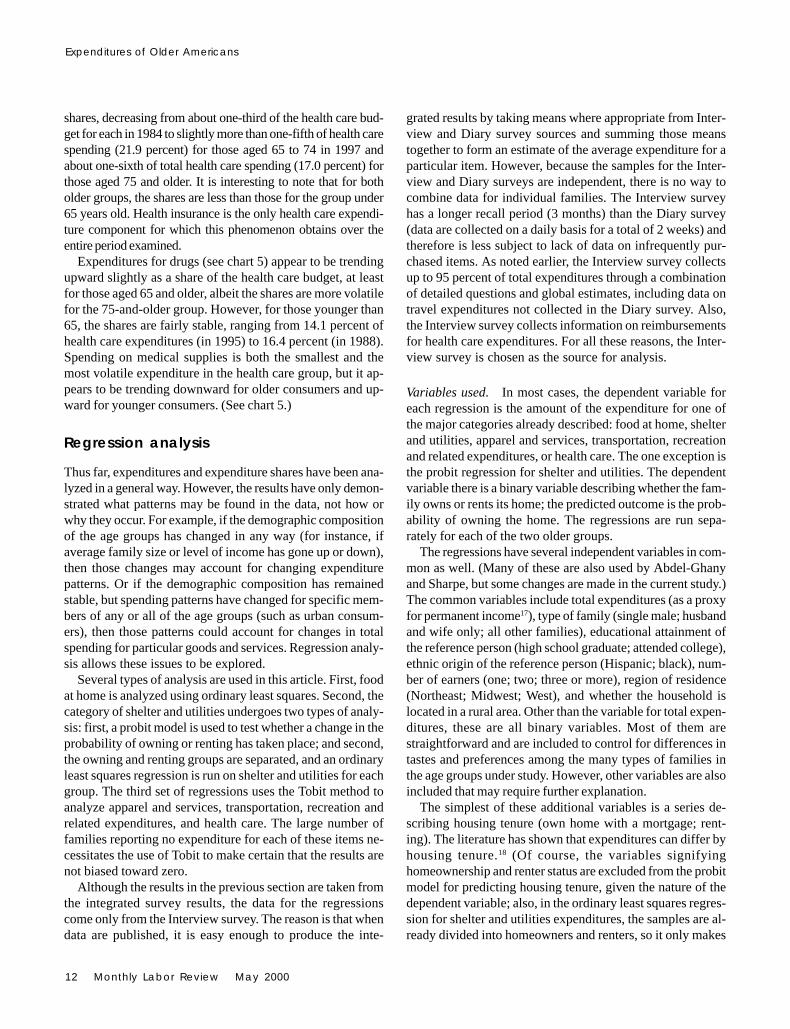
Table 1 shows that, while younger families have had rela-tively stable expenditure levels in real (that is, adjusted forinflation) dollars from 1984 to 1997, real expenditures (in 1997dollars) by older consumers have risen substantially—14 per-cent for those aged 65 to 74 and 18 percent for those aged 75and older. As a result, spending by older consumers has risenfrom 12.6 percent to 14.6 percent of all consumer spending.(See chart 1.) Put another way, those 65 and older once ac-counted for 1 in every 8 consumer dollars spent; now theyaccount for more than 1 in every 7 consumer dollars spent.13

Of course, this rise in aggregate consumer spending sharemay reflect the phenomenal growth rate in the stock marketduring the period in question, given that older consumers aremore likely than younger consumers to live on proceeds fromselling assets or on dividends and other income that assetsproduce.

But what are the ramifications for less aggregated expendi-tures? Surely, if older consumers have different tastes, prefer-ences, or physical needs than younger consumers, they areexpected to have differences in expenditure patterns. To testthis idea, trends for several major expenditure categories, in-cluding food at home, housing (shelter and utilities),14 ap-parel, transportation, and recreation (including entertainment,food away from home, and reading) are displayed in real (thatis, inflation-adjusted) terms. (See chart 2.) In each of thesecases, indeed, older consumers purchase different amountsthan younger consumers, but in most cases, the trend of ex-penditures is similar for older and younger consumers. Oneinteresting exception is recreation: although all age groupsexhibited a real decrease in these expenditures during the1990–91 recession, in 1997, recreation expenditures of youngerconsumers were down slightly (about 1 percent) from their1991 value, whereas they had risen substantially for olderconsumers by 1997—19 percent for those aged 65 to 74 and28 percent for those at least 75 years old.



An analysis of shares is also useful in this case. Aggregateshares, or the percentage of total consumer spending on aparticular category for which each age group accounts, areespecially enlightening, because they provide insight intowhich sectors are changing with the population. Older con-sumers are indeed accounting for larger shares of most of themajor expenditures. (Only the share for food at home remainedrelatively stable for all age groups.) This trend is largely at-tributable to changes in aggregate expenditure shares forthose who are 75 and older. For example, in 1984, that groupaccounted for 5 percent of spending on shelter and utilities, ashare that steadily increased to nearly 7 percent in 1993. Al-though it has since declined to about 6 percent, the overallaggregate share for shelter and utilities for those aged 65 andolder rose from about 14 percent to 15 percent from 1984 to1997.

Similarly, the older group accounted for 2.6 percent of totalspending on apparel in 1984, but the share rose to 4.0 percent

in 1997. The rise means that consumers who are at least 65years old have increased their share of spending on apparelfrom 1 in every 10 dollars to 1 in every 8 dollars.

For those aged 75 and older, the change in transportationshares are identical to the change in apparel shares from 1984-1997. (That is, they rise from 2.6 percent to 4.0 percent overthe period.) However, the aggregate expenditure share forthose aged 65 to 74 has been fairly stable, ranging from a lowof 7.8 percent in 1987 to a high of 9.3 percent in 1988, butusually staying between 8 percent and 9 percent. Therefore,the aggregate share for the combined older groups increasedfrom 10.9 percent to 12.3 percent of total consumer spendingon transportation.

Aggregate shares for recreation increased for all older con-sumers. For those aged 65 to 74, the aggregate share increasedfrom 7.6 percent to 8.7 percent from 1984 to 1997. Again, theincrease was even greater for those aged 75 and older, risingfrom 2.9 percent to 4.5 percent. Altogether, this group’s share

Selected characteristics of families, by age group, 1984–97

Item 1984 1985 1986 1987 1988 1989 1990 1991 1992 1993 1994 1995 1996 1997

Number ofhouseholds(thousands):Under age 65 72,357 72,919 74,727 74,378 75,259 75,496 76,889 77,216 78,256 78,189 80,709 81,330 82,659 83,640 15.665 to 74 ........ 10,761 11,302 10,832 11,578 11,319 11,848 11,318 11,935 11,959 11,934 12,038 11,933 11,742 12,109 12.575 and older . 7,105 7,343 8,485 8,194 8,284 8,474 8,761 8,767 9,804 9,926 9,463 9,860 9,811 9,827 38.3

Nominal values

Income beforetaxes:1

Under age 65 $25,770 $27,493 $28,036 $30,273 $31,351 $34,447 $35,293 $37,633 $37,465 $38,699 $39,801 $40,878 $42,076 $44,135 71.365 to 74 ........ 15,720 18,191 17,874 18,598 20,704 22,051 21,501 22,723 23,182 24,468 24,934 25,553 25,824 27,492 74.975 and older . 11,712 12,306 12,461 12,912 13,707 16,285 15,435 16,247 18,051 17,192 19,616 18,006 18,379 19,425 65.9

Average annualexpenditures:Under age 65 $23,953 $25,406 $26,113 $26,616 $28,142 $30,190 $30,955 $32,274 $32,423 $33,325 $34,186 $34,949 $36,342 $37,545 56.765 to 74 ........ 15,842 17,938 17,506 18,888 20,120 21,152 20,901 22,564 22,862 23,706 25,059 25,277 27,739 27,792 75.475 and older . 11,122 13,012 12,198 12,230 13,339 15,919 15,450 15,782 17,794 18,350 19,280 18,572 19,603 20,279 82.3

Consumer PriceIndex for AllUrbanConsumers(1982–84 = 100),annualaverage ........... 103.9 107.6 109.6 113.6 118.3 124.0 130.7 136.2 140.3 144.5 148.2 152.4 156.9 160.5 54.5

Real values(1997 dollars)

Income beforetaxes:1


Average annualexpenditures:1


1Complete income reporters only.

Percentchange,1984–97

Table 1.


rose from 10.6 percent of total recreation spending to 13.2percent.

However, the question again arises: Are these changesobserved because of underlying changes in the demographyof the population or because of changing tastes within differ-ent age groups? To answer this question, it is useful to ana-lyze budget shares; that is, we seek to answer the question:What proportion of total expenditures does the average con-sumer unit in a given age group allocate to a given category ofexpenditures? For food at home, all age groups experienced adecrease of about 1 percent to 2 percent in the size of theirbudget share. (For those younger than 65, the share droppedfrom 15 percent to 14 percent; for those 65 and older, the sharestarted at about 11 percent and dropped to 9 percent or 10percent, depending on which subgroup one is considering.)Similarly, changes in shares for apparel, shelter and utilities,transportation, and recreation were minimal. Hence, becausethe budget shares did not change much over time, it is pos-sible to attribute changes in aggregate shares to demographicchanges, rather than changes in taste, within the age groups.

One category of spending merits special attention: healthcare. This category is important for several reasons. First,health care expenditures are expected to be positively corre-lated with age for adults. Second, much work examining vari-ous aspects of health care with data from the Consumer Ex-

penditure Survey has been completed. As noted earlier, worksby Hitschler, Abdel-Ghany and Sharpe, and Rubin andNieswiadomy examined health care for older consumers atleast to some degree. Abdel-Ghany and Sharpe compared ex-penditures of those aged 65 to 74 years and those 75 yearsand older), while both Hitschler, on the one hand, and Rubinand Nieswiadomy, on the other, examined expenditures foreach of these age groups at fixed times—1980 and 1990, forexample. Gregory Acs and John Sabelhaus examined trends inhealth care expenditures from 1980 to 1992, although theirfocus was on nonelderly households “because most of themhave private insurance, while elderly households generallyreceive insurance through medicare coverage.”15

Health care expenditures16 have risen substantially for allgroups since 1984. In real terms, those younger than 65 spentabout 9 percent more in 1997 than they did in 1984. However,those older than 75 spent more than 20 percent more, andthose aged 65 to 74 spent in excess of 26 percent more. Asshown in chart 3, older consumers routinely account for amuch larger share of aggregate consumer spending on healthcare than their share of the population. For example, in 1997,those 65 years and older, making up only a bit more thanone-fifth of the total population, accounted for nearlyone-third of total health care expenditures.

But how are health care dollars allocated? Have there been

1984 1985 1986 1987 1988 1989 1990 1991 1992 1993 1994 1995 1996 1997

0

5

10

15

20

0

5

10

15

20

65 and over65-7475 and over

Percent Percent

Chart 1. Share of total expenditure accounted for by older consumers



1984 1985 1986 1987 1988 1989 1990 1991 1992 1993 1994 1995 1996 19970

1,000

2,000

3,000

4,000

5,000

6,000

7,000

0

1,000

2,000

3,000

4,000

5,000

6,000

7,000

Under 6565 7475 and older

Expenditure Expenditure

Chart 2. Expenditures of older consumers for selected services,1997 dollars

Food at home

1984 1985 1986 1987 1988 1989 1990 1991 1992 1993 1994 1995 1996 19970

2,500

5,000

7,500

10,000

0

2,500

5,000

7,500

10,000


Expenditure ExpenditureShelter and utilities

1984 1985 1986 1987 1988 1989 1990 1991 1992 1993 1994 1995 1996 19970

500

1,000

1,500

2,000

2,500

0

500

1,000

1,500

2,000

2,500


Apparel and servicesExpenditure Expenditure

$ $

$$

$ $


any changes in the way older consumers spend their health carebudgets? Shares analysis provides some insight. To start with,health expenditure shares are most volatile for those aged 75and older. (See chart 4.) For the years 1984 to 1997, as a share oftotal expenditures, they ranged from a low of 12.7 percent in 1985to a high of 16.7 percent in 1988. By contrast, for those betweenthe ages of 65 and 74, the share of total expenditures allocated tohealth care stayed between 8.9 percent (in 1987) and 11.0 per-cent (in 1993). For those younger than 65, the range was narrow-est, from 3.8 percent (from 1985 to 1987) to 4.5 percent (in 1993).

All groups, however, experienced changes in how their healthcare dollars were spent: a larger share of the health care budgetwent to health insurance in 1997 than in 1984, regardless of the

group considered. (See chart 5.) Although those aged 65 andolder consistently allocated a larger share of their health carebudget to insurance than those younger than 65, the trend wassimilar for each group. Those younger than 65 allocated lessthan one-third of their health care budget (32.8 percent) to healthinsurance in 1984, compared with nearly half (45.2 percent) in1997. Those aged 65 to 74 increased their share from 44 percentin 1984 to 53.3 percent in 1997, and the share rose even more forthose aged 75 and older, going from 37.9 percent in 1984 to 53.4percent in 1997.

The increased share for health insurance may explain the con-comitant decrease in shares for medical services. (See chart 5.)Again, the two older age groups experienced similar changes in

1984 1986 1988 1990 1992 1994 19960

1,500

3,000

4,500

6,000

7,500

9,000

0

1,500

3,000

4,500

6,000

7,500

9,000Under 6565 7475 and older

Expenditure Expenditure

Chart 2. Continued--Expenditures of older consumers for selected services, 1997 dollars

Transportation

1984 1986 1988 1990 1992 1994 19960

1,500

3,000

4,500

6,000

0

1,500

3,000

4,500

6,000Under 6565 7475 and older

Expenditure ExpenditureRecreation

$ $

$$



1984 1985 1986 1987 1988 1989 1990 1991 1992 1993 1994 1995 1996 19970

5

10

15

20

25

30

35

40

0

5

10

15

20

25

30

35

40

Aggregate health care expendituresPopulation

Percent Percent

Chart 3. Share of aggregate health care expenditures and total population for consumers 65 and older, 1984–97

1984 1985 1986 1987 1988 1989 1990 1991 1992 1993 1994 1995 1996 1997

0

2

4

6

8

10

12

14

16

18

20

0

2

4

6

8

10

12

14

16

18

20Under 6565 74

75 and older

Percent Percent

Chart 4. Health care as a share of total expenditures of elderly, 1984–97


1984 1986 1988 1990 1992 1994 19960

10

20

30

40

50

60

70

Under 6565 7475 andolder

Percent

Chart 5. Selected health services as percent of total expenditures for health care, 1984–97

Health insurance Percent Medical services

1984 1986 1988 1990 1992 1994 19960

5

10

15

20

25

30


Percent Drugs

1984 1986 1988 1990 1992 1994 19960

2

4

6

8

10


Percent Medical supplies

1984 1986 1988 1990 1992 1994 19960

10

20

30

40

50

60

Under 65

65 74

75 and older



shares, decreasing from about one-third of the health care bud-get for each in 1984 to slightly more than one-fifth of health carespending (21.9 percent) for those aged 65 to 74 in 1997 andabout one-sixth of total health care spending (17.0 percent) forthose aged 75 and older. It is interesting to note that for botholder groups, the shares are less than those for the group under65 years old. Health insurance is the only health care expendi-ture component for which this phenomenon obtains over theentire period examined.

Expenditures for drugs (see chart 5) appear to be trendingupward slightly as a share of the health care budget, at leastfor those aged 65 and older, albeit the shares are more volatilefor the 75-and-older group. However, for those younger than65, the shares are fairly stable, ranging from 14.1 percent ofhealth care expenditures (in 1995) to 16.4 percent (in 1988).Spending on medical supplies is both the smallest and themost volatile expenditure in the health care group, but it ap-pears to be trending downward for older consumers and up-ward for younger consumers. (See chart 5.)

Regression analysis

Thus far, expenditures and expenditure shares have been ana-lyzed in a general way. However, the results have only demon-strated what patterns may be found in the data, not how orwhy they occur. For example, if the demographic compositionof the age groups has changed in any way (for instance, ifaverage family size or level of income has gone up or down),then those changes may account for changing expenditurepatterns. Or if the demographic composition has remainedstable, but spending patterns have changed for specific mem-bers of any or all of the age groups (such as urban consum-ers), then those patterns could account for changes in totalspending for particular goods and services. Regression analy-sis allows these issues to be explored.

Several types of analysis are used in this article. First, foodat home is analyzed using ordinary least squares. Second, thecategory of shelter and utilities undergoes two types of analy-sis: first, a probit model is used to test whether a change in theprobability of owning or renting has taken place; and second,the owning and renting groups are separated, and an ordinaryleast squares regression is run on shelter and utilities for eachgroup. The third set of regressions uses the Tobit method toanalyze apparel and services, transportation, recreation andrelated expenditures, and health care. The large number offamilies reporting no expenditure for each of these items ne-cessitates the use of Tobit to make certain that the results arenot biased toward zero.

Although the results in the previous section are taken fromthe integrated survey results, the data for the regressionscome only from the Interview survey. The reason is that whendata are published, it is easy enough to produce the inte-

grated results by taking means where appropriate from Inter-view and Diary survey sources and summing those meanstogether to form an estimate of the average expenditure for aparticular item. However, because the samples for the Inter-view and Diary surveys are independent, there is no way tocombine data for individual families. The Interview surveyhas a longer recall period (3 months) than the Diary survey(data are collected on a daily basis for a total of 2 weeks) andtherefore is less subject to lack of data on infrequently pur-chased items. As noted earlier, the Interview survey collectsup to 95 percent of total expenditures through a combinationof detailed questions and global estimates, including data ontravel expenditures not collected in the Diary survey. Also,the Interview survey collects information on reimbursementsfor health care expenditures. For all these reasons, the Inter-view survey is chosen as the source for analysis.

Variables used. In most cases, the dependent variable foreach regression is the amount of the expenditure for one ofthe major categories already described: food at home, shelterand utilities, apparel and services, transportation, recreationand related expenditures, or health care. The one exception isthe probit regression for shelter and utilities. The dependentvariable there is a binary variable describing whether the fam-ily owns or rents its home; the predicted outcome is the prob-ability of owning the home. The regressions are run sepa-rately for each of the two older groups.

The regressions have several independent variables in com-mon as well. (Many of these are also used by Abdel-Ghanyand Sharpe, but some changes are made in the current study.)The common variables include total expenditures (as a proxyfor permanent income17), type of family (single male; husbandand wife only; all other families), educational attainment ofthe reference person (high school graduate; attended college),ethnic origin of the reference person (Hispanic; black), num-ber of earners (one; two; three or more), region of residence(Northeast; Midwest; West), and whether the household islocated in a rural area. Other than the variable for total expen-ditures, these are all binary variables. Most of them arestraightforward and are included to control for differences intastes and preferences among the many types of families inthe age groups under study. However, other variables are alsoincluded that may require further explanation.

The simplest of these additional variables is a series de-scribing housing tenure (own home with a mortgage; rent-ing). The literature has shown that expenditures can differ byhousing tenure.18 (Of course, the variables signifyinghomeownership and renter status are excluded from the probitmodel for predicting housing tenure, given the nature of thedependent variable; also, in the ordinary least squares regres-sion for shelter and utilities expenditures, the samples are al-ready divided into homeowners and renters, so it only makes


sense to include mortgage status in the owner group andto omit the renter variable entirely.) Another additionalvariable controls for the size of the household when threeor more members are present. Why control only for thiscircumstance? By definition, single-member householdsinclude only one person; similarly, families consisting of ahusband and wife only include two members. The effectsof the size and type of family are therefore encapsulated inone variable, at least for these situations. Other familiescan consist of two members (such as a grandparent andgrandchild) or more. For these cases, the effects of familysize and type can be (and are) disentangled. Finally, a se-ries of interaction terms is included to test whether thereare changes from 1984 to 1997 in the relationship of theselected expenditures to any of the independent variables,including permanent income.

Model-specific variables. In a few cases, certain variablesare of obvious use in predicting a particular type of expendi-ture, but may not be so important in predicting other expendi-tures. For example, expenditures on transportation clearly areexpected to vary with the number of vehicles owned, but it isnot clear whether expenditures for apparel and services doso. Similarly, variables accounting for the number of rooms(including bedrooms), bathrooms, and half bathrooms areincluded in each of the housing regressions (excluding theprobit model, because it is the characteristics of the family,and not the dwelling, that are of interest in that case). Finally,in the model for health care expenditures, variables are in-cluded to describe whether or not the family received a reim-bursement for any component of health care spending (medi-cal services, prescription drugs, or medical supplies). Reim-bursements are treated as negative expenditures for the quar-ter in which they are received; therefore, they lower totalhealth care expenditures for that quarter. Because the Con-sumer Expenditure Survey does not collect information onwhether reimbursements are expected in the future, it is notpossible to include a variable to minimize the effect of poten-tially large expenditures for health care that will eventually bereimbursed.

Finally, in the ordinary least squares models for shelter andutilities, variables for the number of earners are omitted. Thereason is that only in 1997 were there any observations forrenters who are at least 75 years old and who have more thanone earner. Therefore, the regression would not be able to berun properly, given that it tests for changes over time in therelationship between expenditures and number of earners.Because these variables were not statistically significant (atleast not at the 95-percent confidence level) for renters be-tween the ages of 65 and 74 or for owners in either age group,the variables were dropped from the ordinary least squaresmodels in order to keep them consistent.

Price changes. Some caution is needed in the interpretationof these results. Before the regressions are computed, all 1984expenditures (including the dependent variables and perma-nent income) are adjusted by the Consumer Price Index (CPI)for all goods and services. This is done to convert the nomi-nal 1984 values into “real” 1997 values. However, not allchanges in prices are adjusted. For example, suppose that theprice of a specific good drops from 1984 to 1997, and there-fore, families purchased more of it during the period. Then thenominal value of the expenditure in 1997 may be higher than,lower than, or the same as it was in 1984, depending on howmuch the price dropped and how much the quantity purchasedincreased. However, if the nominal value of the expenditurefor the good in 1984 is divided by its price in 1984 and theresult is multiplied by the good’s price in 1997, then the nomi-nal expenditure in 1997 will be greater than the “real” (that is,price-adjusted) value for 1984 (because the adjustment holdsprices constant and the quantity purchased increased). Thedrawback of this method is that information on the price of thegood may not be readily available. However, if a CPI value isavailable for that specific good, then the 1984 expenditure canbe divided by the 1984 CPI for the good and multiplied by its1997 counterpart. The resulting percent change in the adjusted1984 expenditure and the observed 1997 expenditure wouldbe the same as calculated by this method or the method ofusing prices directly. In either case, the 1984 nominal expendi-ture would be converted to a real 1997 expenditure for theselected good. However, the CPI for all goods and servicesdid not drop from 1984 to 1997; instead, the combined pricesof all goods and services rose over that period. Therefore,adjusting the expenditure by the change in the overall CPI willnot have the same effect as adjusting by the specific good’sindex! (If a good doubles in price and the quantity purchasedfalls by less than 50 percent, the nominal expenditure stillrises, even though less is purchased.) Then what is the rea-son for adjusting specific expenditures by the overall pricechange? First, no indexes are readily available for some of thegoods and services that are examined. (The category of recre-ation and related expenditures is one example.) Second, ad-justing by the overall CPI still has the advantage of at leastcontrolling for general price changes. For suppose that, inreal terms (that is, adjusting by the overall CPI), the expendi-ture for a specific item has doubled. Then it can be said withcertainty that the average family of interest is allocating twicethe purchasing power to the good or service in question thatit did in the earlier period. Again, we do not know whetherprice or quantity changes in the later period account for thisincrease, but we do know that, in real terms, the expendituremakes up a larger share of the budget in 1997 than it did in1984.

These results should be kept in mind when one is interpret-ing such factors as the marginal propensity to consume (MPC)



and the (permanent) income elasticity of the selected expendi-tures. The conventional interpretation of the MPC is that itrepresents the fraction of each additional dollar that would beallocated toward the purchase of the good in question, as-suming that the family under study received an additionaldollar from some source. Implicit in this statement is that in-creased expenditures are a result of increased quantities pur-chased. However, in the present case, all that can be said forsure is that if the MPC is found to increase over time, then alarger share of the dollar is being spent on the good or ser-vice, but again, it is not clear whether this is because pricesincreased or whether it is because quantities increased. Simi-larly, income elasticity is usually interpreted to mean the per-cent increase (or decrease) in the quantity purchased, given a1-percent increase in income. However, in the present circum-stances, it is interpreted as the percent increase in expendi-ture (in constant 1997 dollars) for the good in question, givena 1-percent increase in income.

Sample issues. Before the regressions are run, familieswhose total health care expenditures are negative (due to re-imbursements) are dropped from the sample. This is done fortwo reasons. First, if included in the health care model, theywould obviously cause a problem when the regression modelwas computed, because a few expenditures would be nega-tive, several would be zero, and most would be positive. It isnot clear how the Tobit model would be specified in such acase. However, as noted earlier, it is at least possible to con-trol for situations in which a reimbursement is received forsome component of health care, but is not enough to make theentire health care expenditure negative. Therefore, to keep thesample as consistent as possible for the regressions, thosefamilies with negative health care expenditures are droppedfrom it. Second, in some cases, the reimbursement is so largethat total expenditures are actually negative. Because totalexpenditures are used as a proxy for permanent income inthese models, eliminating negative health care expendituresensures that total expenditures will not be negative.

Similarly, a small percentage of families have no value re-ported for the number of rooms. Because this situation affectsonly the housing models, these families are omitted just fromthat sample.

For 1984, the models include 2,341 observations for the 65-to 74-year-old group and 1,609 for the 75-and-older group. In1997, there were 2,436 observations for the 65- to 74-year-oldgroup and 2,076 for the 75-and-older group. The models arespecified to show how relationships between expendituresand characteristics changed over the period for each group.Within each age group, the data for both years are combined,yielding a total of 4,777 observations for the models that in-clude the 65- to 74-year-old group and 3,685 for those thatinclude the 75-and-older group. (For the housing regressions,

the sample is 4,710 for the first age group and 3,652 for thesecond age group.)

The control group. In analyzing the results of the regres-sion techniques, a control group to which families with differ-ing characteristics can be compared was defined. Conven-tionally, the control group is designed to represent a “typical”sample point. For example, regardless of the year or age group,the majority of older families studied have no earner present.Therefore, one of the characteristics of the “typical” family isthat it has no earners. In some cases, some judgment must beused to decide what represents the “typical” family. For ex-ample, regardless of the year, single persons constitute themajority of families who are in the second age group. (Seetable 2.) However, for the first age group, married couples(with no other members present) are the more typical arrange-ment, accounting for 3 out of 7 households, regardless of theyear. Nevertheless, earlier it was shown how family type andfamily size interrelate. Using singles as the control group,then, provides a logical base on which to build—a marriedcouple is not only a different family type, but it includesexactly one more person than a single family, so the differ-ence in expenditures due to adding an extra person to thefamily is subsumed in the coefficient for married couples.Furthermore, because most of the singles are female, by speci-fying single females as members of the control group, differ-ences in tastes for single men and women can be measuredby including a variable to indicate whether the family is com-posed of a single male.

Accordingly, the control group for each regression is madeup of families whose reference person is a single female whois (1) not a high school graduate, (2) neither Hispanic norblack, (3) not an earner, (4) a homeowner with no mortgage(except in the regression for shelter and utilities for renters),and (5) living in an urban area in the South. For the purposesof estimating factors such as income elasticity, families areassumed to have average characteristics for their age groupwhere continuous variables (such as total expenditures ornumber of rooms) are concerned. The control group appliesto each age group and each year. Although such a householdmay not exist, coefficients for other characteristics are shownso that estimates of expenditures or other factors can be com-puted for whatever group is examined.

A few words on Tobit. Tobit regression is used when thereare a substantial number of nonexpenditures reported (as inthis study). In other words, if a family did not purchase anitem, then the expenditure on that item is recorded as zerodollars.19 As pointed out in Abdel-Ghany and Sharpe, includ-ing these zeros without some sort of adjustment would yieldbiased results. In such cases, Tobit is useful because it is atwo-stage regression procedure. The first stage predicts the


Selected characteristics to accompany regression results

1984 1997 1984 1997

Sample size ....................................................................................... 2,341 2,436 1,609 2,076Homeowners ..................................................................................... 1,804 1,952 1,096 1,571Reporting number of rooms ............................................................ 1,765 1,897 1,059 1,507Missing rooms, bathrooms, or half baths ....................................... 39 55 37 64

Renters ............................................................................................ 537 484 513 505Reporting number of rooms ............................................................ 515 461 495 493Missing rooms, bathrooms, or half baths ....................................... 22 23 18 12

Percent reporting expenditures:Total (quarterly) ................................................................................ 100.0 100.0 100.0 100.0Food at home ................................................................................... 99.6 99.6 99.8 99.8Shelter and utilities:Homeowners (room reporters only) ................................................ 99.8 100.0 99.8 100.0Renters (room reporters only) ........................................................ 100.0 100.0 100.0 100.0

Apparel and services ....................................................................... 84.5 78.7 70.0 67.3Transportation .................................................................................. 91.4 93.7 72.1 80.6Recreation and related items ........................................................... 92.0 94.7 84.5 91.5Health care ....................................................................................... 96.0 97.8 96.2 98.8

Characteristics (percent)Family composition:Single man ..................................................................................... 7.9 9.2 9.6 10.6Single woman ................................................................................. 26.9 27.2 47.3 44.3Husband and wife only ................................................................... 42.3 41.9 27.7 30.6Other family ................................................................................... 22.9 21.7 15.5 14.5

Three or more members ................................................................... 14.4 14.7 5.9 5.3Reference person:Educational attainment:Less than high school .................................................................. 48.2 31.9 63.0 39.4High school graduate ................................................................... 28.8 32.8 16.8 31.4Attended college .......................................................................... 23.0 35.3 20.3 29.2

Ethnic origin:Hispanic ....................................................................................... 3.3 5.5 2.2 3.2Black ............................................................................................ 6.0 9.7 5.8 5.3White or other .............................................................................. 90.7 84.8 92.0 91.5

Number of earners:Zero .............................................................................................. 58.6 58.0 84.2 83.0One .............................................................................................. 28.5 28.9 13.0 14.0Two ............................................................................................... 10.3 10.4 2.1 2.6Three or more ............................................................................... 3.0 2.3 .7 .4

Mortgage status:Has mortgage ............................................................................... 17.9 19.2 4.4 8.9No mortgage (owners only) ......................................................... 59.2 61.0 63.7 66.8

Region of residence:Northeast ..................................................................................... 25.2 22.0 26.3 18.4Midwest ........................................................................................ 25.8 28.3 28.7 27.6South ............................................................................................ 28.8 31.4 28.2 33.1West ............................................................................................. 20.1 18.3 16.8 20.9

Living in rural areas ........................................................................ 14.8 11.9 15.1 10.9

Receiving reimbursement for health care ....................................... 1.9 1.1 1.6 1.0

Average number reported:Rooms .......................................................................................... 5.4 5.7 5.0 5.3Homeowners ............................................................................... 5.9 6.1 5.5 5.8Renters ....................................................................................... 3.9 4.1 3.9 3.8

Bathrooms ...................................................................................... 1.3 1.4 1.2 1.3Homeowners ................................................................................. 1.3 1.5 1.2 1.4Renters ........................................................................................ 1.0 1.1 1.0 1.1

Half bathrooms ............................................................................... .2 .3 .2 .2Homeowners ................................................................................. .3 .4 .2 .3Renters ........................................................................................ (1) .1 .1 .1

Vehicles .......................................................................................... 1.5 1.8 .8 1.2

1 Less than 0.05.

Table 2.

Characteristic65–to–74 age group 75–and–older age group



probability of purchase of a given item (using a probit tech-nique), and the second stage predicts how much is spent onthe item, assuming that it is in fact purchased. However, Tobitcoefficients cannot be interpreted in the same way as ordi-nary least squares coefficients, because a change in one ofthe independent variables (say, an increase in permanent in-come) may influence the outcome not only by increasing theamount of the purchase, but also by influencing the probabil-ity of making the purchase in the first place.20 The properadjustments are made in each case before calculating MPCsand income elasticities for results from Tobit regressions.

In using regression results to estimate income elasticities,it is necessary to have a value both for expenditures for thegood or service under study and for total expenditures (per-manent income). The data from the Interview survey are avail-able in a quarterly format. For regression purposes, each quar-ter is treated independently, although the same family mayappear more than once in the sample. Because of the quarterly

availability, expenditures in table 3 are quarterly averages forthe year in which the consumer unit participated in the inter-view.21 For purposes of evaluation, the control group is as-sumed to have average quarterly expenditures at both theaggregate (that is, total expenditures) and the component (forexample, food at home) level. In the Tobit regressions, though,expenditures for specific goods and services (apparel andservices, transportation, recreation and related items, andhealth care) are not quarterly averages, but are predicted quar-terly expenditures for a member of the reference group. Again,this is because Tobit results require special adjustments be-fore interpretation, and it is necessary to use predicted expen-ditures to obtain elasticity estimates.

Food at home. At least for those 65 to 74 years old, relation-ships between characteristics and expenditures appear tohave been remarkably stable over time. Although severalcharacteristics have statistically significant parameter esti-

Results derived from regression analyses, by age group

65–to–74 age group 75–and–older age group

1984 1997 1984 1997

Total expenditures (quarterly) ..................................... $6,016 $6,513 $3,962 $4,922

Food at home: Expenditure ............................................................. $813 $782 $568 $615 Marginal propensity to consume .............................. 1.030 1.020 1.020 1.016 Income elasticity ..................................................... .222 .167 .140 .128

Shelter and utilities, owners: Expenditure ............................................................. $1,358 $1,561 $1,150 $1,275 Marginal propensity to consume .............................. 1.072 1.059 1.047 1.065 Income elasticity ..................................................... .319 .246 .162 .251

Shelter and utilities, renters: Expenditure ............................................................. $1,241 $1,572 $1,221 $1,588 Marginal propensity to consume .............................. 1.094 .081 1.119 1.189 Income elasticity ..................................................... .456 .336 .386 .586

Tobit results

Apparel and services: Expenditure (predicted) ........................................... $270 $222 $119 $107 Marginal propensity to consume .............................. 1.023 .018 1.007 1.012 Income elasticity ..................................................... .512 .528 .233 .552

Transportation: Expenditure (predicted) ........................................... $1,710 $1,511 $438 $587 Marginal propensity to consume .............................. 1.321 1.240 1.035 1.093 Income elasticity ..................................................... 1.129 1.034 .317 .780

Recreation and related items: Expenditure (predicted) ........................................... $556 $606 $393 $561 Marginal propensity to consume .............................. 1.066 1.057 1.031 1.059 Income elasticity ..................................................... .714 .613 .313 .518

Health care: Expenditure (predicted) ........................................... $612 $708 $700 $708 Marginal propensity to consume .............................. 1.028 1.042 1.053 1.020 Income elasticity ..................................................... .275 .386 .300 .139

Model and category

1Indicates that the coefficient for the marginal propensity to consume isstatistically significant at the 95-percent confidence level. For 1984, thismeans that the marginal propensity to consume is significantly different from

zero. For 1997, this means that the marginal propensity to consume is signifi-cantly different than it was in 1984.

Table 3.


mates, none of these variables has a statistically significantparameter estimate when interacted with the binary variablewhich indicates that the data are from 1997 (table 4). In otherwords, some characteristics, such as type of family and re-gion of residence (at least, the Northeast) appear to have abearing on food-at-home expenditures for the 65- to 74-year-old group, but these relationships do not appear (at the 95-percent confidence level) to have changed over time. For those75 and older, however, a few changes are noted. First, familieswith multiple members appear to have spent less for food athome in 1997 than they did in 1984, as did families in theMidwest. Families with more than one earner, however, ap-peared to have spent more, as the coefficients for bothtwo-earner and multiple-earner families are statistically sig-nificant for 1997 (but not for 1984). The intercept also increasedin 1997 for the 75-and-older group (but not for the 65- to 74-year-olds), indicating that expenditures were higher for thecontrol group in 1997.

For both age groups, though, the MPC decreased, as shownin table 3. This is consistent with the increase in expendituresfor food away from home for both groups. Note that althoughtotal expenditures for the older group increased by a largerproportion (24 percent) than food expenditures (8 percent), afact that, all other things being equal, would increase the in-come elasticity of food expenditures, the decrease in the MPC

was enough to offset these changes and to cause the elastic-ity to fall, if slightly.

Shelter and utilities. Regardless of the year, the majority ofcontrol group members are predicted to be homeowners. Infact, the predicted values are remarkably similar for each agegroup, regardless of the year, despite the higher predictedprobability of ownership for each group in 1997. In 1984, forexample, the predicted probability of ownership for 65- to 74-year-olds is 58 percent, compared with 56 percent for the 75-or-older group. In 1997, the probability increases to 72 per-cent for the former and 76 percent for the latter.22 In neitherage group is the intercept (indicating a “base” probability for1984) statistically significant, although for each of them, thecoefficient for 1997 is positive and statistically significant atthe 99-percent confidence level. The income parameter is sta-tistically significant (again at the 99-percent level) for the 65-to 74-year-old group in 1984, but there is no significant changein the relationship between their probability of owning andpermanent income for 1997. For the 75-and-older group, theincome effect is not statistically significant in 1984,23 and thereis no evidence of a change in the relationship by 1997. House-holds consisting of a husband and wife only are more likely toown than are single females in either year, regardless of theage group. Similarly, families with three or more members aremore likely to own, regardless of the year.24 Probability ofownership increases with education for the younger age

group, but not for the older. However, the probability of own-ership is lower for Hispanics in each age group and for blacksin the older group, but not for blacks in the younger group.Probability of ownership also decreases significantly forNortheasterners in 1997, although it is higher for rural familiesin each year. (See table 5.)

Expenditure patterns for owners show different changesby age group in each year. For example, for 65- to 74-year-oldsin 1997, both the intercept and the income coefficient decreasesignificantly. (See table 6.) However, for those 75 and older in1997, both coefficients increase, although the change in theintercept is not statistically significant. Note that for the lattergroup, these changes, coupled with the aforementioned in-crease in total expenditures (24 percent) and a smaller increasein shelter and utilities expenditures (11 percent), contribute toa substantial increase in income elasticity for owners in thegroup. However, for the younger group, estimated incomeelasticity is substantially lower for 1997 than for 1984. Again,the opposite of the older group holds for the younger group:a smaller MPC in 1997 is accompanied by an increase in totalexpenditure (8 percent) that is smaller than the percent in-crease in expenditures for shelter and utilities (15 percent), allof which act to make the elasticity for the group smaller in1997 than 1984.

For renters in both age groups, expenditure patterns areremarkably stable. For both age groups, expenditures appearto have increased in 1997 for those who attended college.(See table 7.) Other than this, the only statistically significantvariables for the 65- to 74-year-old group in 1997 are familysize (multiple members) and regional variables; expendituresfor this group appear to have risen for residents of the Mid-west and West. For those 75 and older, the intercept is signifi-cantly larger in 1997, as is the MPC. Also, the coefficient fornumber of bathrooms is statistically significant (and nega-tive) for 1997. Both age groups are fairly homogeneous, withfew other parameter estimates being statistically significant,regardless of the year. For the younger age group, only coef-ficients for family type (husband and wife only; other fami-lies), rural residence, and number of rooms are statisticallysignificant. The rural coefficient is negative, but the othersare positive. For the older group, living in a rural area is alsoassociated with lower expenditures, while the numbers ofbathrooms and half bathrooms appear to increase expendi-tures for housing for this group.

Although these expenditures are similar for each age groupin each year, MPCs and elasticities are quite different for eachgroup of renters and, in fact, change differently over time.(See table 3.) For the younger age group, the MPC for 1997does not differ from that for 1984 in any statistically signifi-cant way. For the older group, however, the MPC increasessubstantially from 1984 to 1997. Despite a similar increase forboth groups in expenditures for shelter and utilities (27 per-



Regression results, food-at-home model

65-to-74 age group 75-and-older age group

Parameter Standard Parameter Standard

Intercept ......................................... 403.101 30.357 13.278 0.000 338.513 24.321 13.918 0.000Interaction, 1997 ......................... –11.200 42.766 –.262 .793 94.069 31.917 2.947 .003

Total expenditures ........................... .030 .002 15.164 .000 .020 .002 10.765 .000Interaction, 1997 ......................... –.010 .003 –3.822 .000 –.004 .002 –1.970 .049

Family composition:Single man ................................... –5.935 37.995 –.156 .876 –8.501 31.038 –.274 .784

Interaction, 1997 ...................... –19.373 52.031 –.372 .710 –28.626 40.560 –.706 .480

Husband and wife only ................ 285.910 25.357 11.276 .000 298.351 22.419 13.308 .000Interaction, 1997 ...................... 31.346 35.033 .895 .371 –43.760 29.579 –1.479 .139

Other family ................................. 250.735 38.796 6.463 .000 256.624 33.671 7.622 .000Interaction, 1997 ...................... 3.104 55.841 .056 .956 –23.902 44.958 –.532 .595

At least three members ............... 399.208 43.666 9.142 .000 336.898 51.675 6.520 .000Interaction: 1997 ..................... –95.512 62.111 –1.538 .124 –262.075 68.098 –3.849 .000

Education of the reference person:High school graduate ................... –36.895 22.863 –1.614 .107 29.567 24.503 1.207 .228

Interaction, 1997 ...................... 28.102 33.007 .851 .395 –75.452 30.809 –2.449 .014

Attended college .......................... –25.177 25.857 –.974 .330 21.562 23.381 .922 .357Interaction, 1997 ...................... 48.397 35.719 1.355 .176 41.324 30.475 1.356 .175

Ethnic origin of the referenceperson:Hispanic ....................................... –56.893 54.281 –1.048 .295 7.585 61.002 .124 .901

Interaction, 1997 ...................... 40.836 68.774 .594 .553 42.735 75.506 .566 .571

Black ........................................... –80.881 41.479 –1.950 .051 –29.130 38.519 –.756 .450Interaction, 1997 ...................... 41.855 52.705 .794 .427 –18.202 52.035 –.350 .727

Number of earners:One earner .................................. –7.551 23.043 –.328 .743 14.929 29.006 .515 .607

Interaction, 1997 ...................... –37.725 32.305 –1.168 .243 70.552 38.168 1.848 .065

Two earners ................................. –43.355 36.701 –1.181 .238 –137.214 71.780 –1.912 .056Interaction, 1997 ...................... –12.542 50.238 –.250 .803 291.068 89.199 3.263 .001

Three or more earners ................. 127.267 64.893 1.961 .050 –164.309 111.276 –1.477 .140Interaction, 1997 ...................... 180.006 95.493 1.885 .060 1150.001 165.953 6.930 .000

Housing tenure:Own home, no mortgage .............. 78.162 26.139 2.990 .003 1.755 44.296 .040 .968

Interaction, 1997 ...................... –9.083 36.161 –.251 .802 50.831 52.364 .971 .332

Renter .......................................... 12.231 24.658 .496 .620 –30.740 20.080 –1.531 .126Interaction, 1997 ...................... 4.793 35.605 .135 .893 –24.359 27.756 –.878 .380

Region of residence:Northeast ..................................... 67.467 26.394 2.556 .011 40.298 24.917 1.617 .106

Interaction, 1997 ...................... 10.329 37.171 .278 .781 –26.421 33.747 –.783 .434Midwest ....................................... –49.656 25.821 –1.923 .055 –11.106 23.869 –.465 .642

Interaction, 1997 ...................... 37.644 35.447 1.062 .288 –71.070 31.118 –2.284 .022

West ............................................ 13.328 28.120 .474 .636 46.241 28.297 1.634 .102Interaction, 1997 ...................... 45.233 39.414 1.148 .251 –28.196 35.704 –.790 .430

Degree of urbanization:Rural ............................................ –42.120 27.580 –1.527 .127 –4.654 25.766 –.181 .857

Interaction, 1997 ...................... 24.677 40.150 .615 .539 –20.702 36.031 –.575 .566

T for H0:parameter = 0estimate error estimate error

T for H0:parameter = 0Prob > |T| Prob > |T|

Variable

Table 4.


Regression results, probability-of-homeownership model


Parameter Standard Parameter Standardestimate error estimate error

Intercept .................................................... –0.064 0.090 0.477 0.062 0.090 0.491 Interaction, 1997 .................................... .389 .129 .003 .521 .123 .000

Total expenditures ...................................... 4.42 X 10-5 1.00 X 10-5 1.00 X 10-4 2.16 X 10-5 1.20 X 10-5 .076 Interaction, 1997 .................................... –6.71 X 10-6 1.30 X 10-5 6.05 X 10-1 8.65 X 10-7 1.50 X 10-5 .954

Family composition: Single man .............................................. –.007 .108 .946 .354 .116 .002 Interaction, 1997 ................................. –.453 .149 .002 –.180 .154 .242

Husband and wife only ........................... .901 .081 .000 .942 .092 .000 Interaction, 1997 ................................. –.216 .115 .061 –.077 .125 .539

Other family ............................................ .183 .114 .110 .592 .131 .000 Interaction, 1997 ................................. .083 .170 .628 –.178 .182 .328

At least three members .......................... .689 .141 .000 .684 .268 .011 Interaction, 1997 ................................. –.370 .203 .068 –.425 .339 .211

Education of the reference person: High school graduate .............................. .191 .075 .011 .144 .098 .144 Interaction, 1997 ................................. .072 .108 .503 –.191 .125 .127

Attended college ..................................... .423 .090 .000 .062 .095 .511 Interaction, 1997 ................................. –.033 .123 .786 -.053 .125 .671

Ethnic origin of the reference person: Hispanic .................................................. –.562 .167 .001 –.658 .223 .003 Interaction, 1997 ................................. .178 .213 .405 –.129 .278 .644

Black ...................................................... –.169 .127 .183 –.513 .147 .001 Interaction, 1997 ................................. –236 .160 .141 .112 .200 .577

Number of earners: One earner ............................................. .067 .077 .387 –029 .121 .808 Interaction, 1997 ................................. –.171 .109 .118 .344 .168 .041

Two earners ............................................ –.069 .130 .597 5.223 2,991.958 .999 Interaction, 1997 ................................. –.006 .186 .976 –5.222 2,991.958 .999

Three or more earners ............................ .651 .348 .062 4.914 4,988.488 .999 Interaction, 1997 ................................. .156 .538 .772 –4.835 4,988.488 .999

Region of residence: Northeast ................................................ –.094 .087 .279 –.251 .099 .011 Interaction, 1997 ................................. –.281 .123 .023 –.292 .135 .031

Midwest .................................................. .064 .086 .456 –.039 .096 .688 Interaction, 1997 ................................. –.016 .122 .895 –.322 .128 .012

West ....................................................... –.090 .094 .341 .035 .113 .755 Interaction, 1997 ................................. –.104 .134 .436 –.294 .146 .044

Degree of urbanization: Rural ....................................................... .229 .091 .012 .302 .108 .005 Interaction, 1997 ................................. .194 .148 .191 –185 .155 .234

Variable

Table 5.

Pr > chi-square

Pr > chi-square

Note: In this form of regression analysis, the standard error of theparameter estimate is drawn from a chi-square distribution. The value "Pr >chi-square" then denotes the level of statistical signigicance of the para-

meter estimate. A value less than or equal to 0.05 indicates statisticalsignificance at the 95-percent confidence level; a value less than or equal to0.01 indicates statistical significance at the 99-percent confidence level.



Regression results, shelter and utilities (owners) model

65–to–74 age group 75–and–older age group

Parameter Standard T for H0: Parameter Standard T for H0:estimate error parameter = 0 estimate error parameter = 0

Intercept ........................................................ 445.260 108.100 4.119 0.000 –54.221 141.541 –0.383 0.702 Interaction, 1997 ....................................... –464.748 152.016 –3.057 .002 170.217 186.836 .911 .362

Total expenditures ......................................... .072 .005 15.302 .000 .047 .006 8.123 .000 Interaction, 1997 ....................................... –.013 .006 –2.049 .041 .018 .007 2.533 .011

Family composition: Single man ................................................. –204.194 110.479 –1.848 .065 106.234 115.604 .919 .358 Interaction, 1997 .................................... 248.420 150.469 1.651 .099 –104.129 147.639 –.705 .481

Husband and wife only .............................. –151.095 63.646 –2.374 .018 35.217 75.355 .467 .640 Interaction, 1997 .................................... 71.138 86.680 .821 .412 –43.215 98.258 –.440 .660

Other family ............................................... –155.225 100.808 –1.540 .124 –33.587 110.621 –.304 .761 Interaction, 1997 .................................... 156.767 140.102 1.119 .263 –115.585 144.753 –.798 .425

At least three members ............................. 52.346 104.176 .502 .615 212.082 146.765 1.445 .149 Interaction, 1997 .................................... 19.861 146.908 .135 .893 –145.753 198.120 -.736 .462

Education of the reference person: High school graduate ................................. 45.294 57.418 .789 .430 113.220 85.050 1.331 .183 Interaction, 1997 .................................... 30.361 82.367 .369 .712 -74.051 106.894 -.693 .489

Attended college ........................................ 157.256 64.214 2.449 .014 140.428 85.810 1.637 .102 Interaction, 1997 .................................... 118.202 89.025 1.328 .184 9.949 109.237 .091 .927

Ethnic origin of the reference person: Hispanic ..................................................... –43.272 151.289 –.286 .775 –287.103 263.950 –1.088 .277 Interaction, 1997 .................................... 108.419 188.687 .575 .566 426.797 320.775 1.331 .184

Black ......................................................... 81.701 115.029 .710 .478 46.369 148.303 .313 .755 Interaction, 1997 ...................................... –129.656 144.343 –.898 .369 101.825 196.315 .519 .604

Region of residence: Northeast .................................................... 353.452 67.104 5.267 .000 471.535 89.669 5.259 .000 Interaction, 1997 ..................................... 224.081 94.348 2.375 .018 3.596 120.512 .030 .976

Midwest ..................................................... 198.275 64.237 3.087 .002 55.688 84.069 .662 .508 Interaction, 1997 .................................... –18.387 87.090 –.211 .833 2.600 108.152 .024 .981

West .......................................................... –54.289 69.890 –.777 .437 43.155 98.091 .440 .660 Interaction, 1997 .................................... 234.287 97.208 2.410 .016 205.410 121.986 1.684 .092

Degree of urbanization: Rural .......................................................... –216.271 68.750 –3.146 .002 –116.735 89.125 –1.310 .190 Interaction, 1997 .................................... 53.357 96.946 .550 .582 96.479 121.391 .795 .427

Housing characteristics: Number of rooms ....................................... –17.867 18.604 –.960 .337 50.018 23.878 2.095 .036 Interaction, 1997 .................................... 54.208 24.381 2.223 .026 –25.294 31.329 –.807 .420

Number of bathrooms ................................ 294.281 50.486 5.829 .000 392.340 69.656 5.633 .000 Interaction, 1997 ..................................... –23.303 66.918 –.348 .728 –146.041 87.581 –1.668 .096

Number of half bathrooms ......................... 126.971 47.143 2.693 .007 73.793 70.116 1.052 .293 Interaction, 1997 .................................... 22.952 62.252 .369 .712 97.979 89.582 1.094 .274

Home owned without mortgage .................. 344.378 57.819 5.956 .000 477.952 127.282 3.755 .000 Interaction, 1997 .................................... 461.323 79.644 5.792 .000 233.220 151.309 1.541 .123

Variable

Prob > |T| Prob > |T|

Table 6.


Regression results, shelter and utilities (renters) model


Parameter Standard T for H0: Parameter Standard T for H0:estimate error parameter = 0 estimate error parameter = 0

Intercept ......................................... 277.627 146.632 1.893 0.059 –280.046 217.740 –1.286 0.199 Interaction, 1997 ......................... –243.468 197.823 –1.231 .219 883.601 270.361 3.268 .001

Total expenditures ........................... .094 .012 8.142 .000 .119 .016 7.554 .000 Interaction, 1997 ......................... –.013 .014 –.979 .328 .070 .020 3.488 .001

Family composition: Single man ................................... 132.063 85.857 1.538 .124 –50.840 141.541 –.359 .720 Interaction, 1997 ...................... 74.820 116.399 .643 .521 134.124 188.141 .713 .476

Husband and wife only ................ 218.094 85.741 2.544 .011 117.967 121.355 .972 .331 Interaction, 1997 ...................... 160.525 120.394 1.333 .183 112.870 175.400 .644 .520

Other family ................................. 225.566 96.576 2.336 .020 72.811 152.779 .477 .634 Interaction, 1997 ...................... 70.161 152.227 .461 .645 41.933 223.120 .188 .851

At least three members ............... –57.687 132.499 –.435 .663 142.728 406.379 .351 .726 Interaction, 1997 ...................... 394.436 192.920 2.045 .041 6.667 496.083 .013 .989

Education of the reference person: High school graduate ................... 106.656 66.696 1.599 .110 212.486 116.709 1.821 .069 Interaction, 1997 ...................... 25.699 98.360 .261 .794 –174.139 148.485 –1.173 .241

Attended college .......................... 92.972 86.613 1.073 .283 189.409 106.645 1.776 .076 Interaction, 1997 ...................... 256.266 117.398 2.183 .029 530.867 149.955 3.540 .000

Ethnic origin of the reference person: Hispanic ....................................... 227.877 119.722 1.903 .057 –111.584 211.851 –.527 .599 Interaction, 1997 ...................... –298.195 159.130 –1.874 .061 –58.818 268.346 –.219 .827

Black ........................................... –160.968 108.217 –1.487 .137 –223.037 159.441 –1.399 .162 Interaction, 1997 ....................... –28.301 133.514 –.212 .832 –152.416 212.867 –.716 .474

Region of residence: Northeast ..................................... 2.179 77.630 .028 .978 94.570 110.298 .857 .391 Interaction, 1997 ...................... 207.025 111.100 1.863 .063 –130.889 156.927 –.834 .404

Midwest ....................................... –23.460 78.132 –.300 .764 43.468 111.086 .391 .696 Interaction, 1997 ...................... 260.096 116.720 2.228 .026 –42.073 156.615 –.269 .788

West ............................................ 143.015 83.572 1.711 .087 92.550 130.487 .709 .478 Interaction, 1997 ...................... 247.338 120.923 2.045 .041 –155.074 176.691 –.878 .380

Degree of urbanization Rural ............................................ –350.615 91.482 –3.833 .000 –323.272 147.021 –2.199 .028 Interaction, 1997 ...................... -83.821 149.703 –.560 .576 –141.411 214.027 –.661 .509

Housing characteristics: Number of rooms ......................... 69.507 24.192 2.873 .004 49.805 31.836 1.564 .118 Interaction, 1997 ...................... 48.391 35.358 1.369 .171 –65.032 45.922 –1.416 .157

Number of bathrooms .................. 195.026 112.982 1.726 .085 809.720 185.694 4.361 .000 Interaction, 1997 ...................... 49.573 144.066 .344 .731 –599.729 208.867 –2.871 .004

Number of half bathrooms ........... 166.061 136.634 1.215 .225 490.383 177.226 2.767 .006 Interaction, 1997 ...................... –160.828 173.546 –.927 .354 –296.626 232.655 –1.275 .203

Variable

Prob > |T|Prob > |T|

Table 7.



cent for the younger and 30 percent for the older), the elastici-ties move in opposite directions. For the younger group, theelasticity falls by more than one-fourth its original value, from0.456 to 0.336. However, for the older group, the elasticityincreases by more than half, from 0.386 to 0.586.

Apparel and services. The 65- to 74-year-old age group ex-hibits remarkably stable and homogeneous expenditure pat-terns for apparel and services. (See table 8.) Single men arepredicted to spend less than single women for these items,and these expenditures also appear to increase with educa-tion. (The coefficient for high school graduates is positiveand statistically significant, and the coefficient for at leastsome college is larger than that for high school graduates andalso statistically significant.) Otherwise, no coefficients arestatistically significant for this expenditure for the youngerage group, regardless of the year.

On the other hand, the group 75 years and older exhibits morediversity in expenditures for apparel and services. Family type(husband and wife only; other families) and family size (multiplemembers) are statistically significant predictors of expenditures.In each case, the main coefficient for the group is positive, withthe 1997 parameter estimate negative. However, the coefficientsvary as to magnitude and statistical significance. For example,the coefficient for husband and wife only is statistically signifi-cant, but the change for 1997 is not. The coefficients for mul-tiple-member households exhibit a similar pattern, except thatthe 1997 coefficient is larger in absolute value than the maincoefficient. It is not statistically significant at the 95-percentconfidence level, but is nearly so. (The p-value is 0.0545.) Theseexpenditures are also predicted to increase with education andto be higher for the Northeast in 1997 than in 1984. Althoughneither the main coefficient nor the 1997 coefficient is statisti-cally significant for two-earner households in the 75-and-oldergroup, expenditures are predicted to be greater for one-earnerand multiple-earner households than for those with no earner.(Both of the coefficients for one-earner families are positive andstatistically significant. For multiple earners, the first is positiveand statistically significant, while the second is negative andnot statistically significant; it is also smaller in absolute valuethan the main coefficient.)

For 65- to 74-year-olds, there is little change in MPC or elastic-ity. (See table 3.) Although slightly lower in 1997, the MPC is notstatistically significantly different that year from it was in 1984.However, for the 75-or-older group, there are notable changes:the MPC nearly doubles, from 0.007 to 0.012, and the elasticitymore than doubles, from 0.233 to 0.552. The proportional re-sponse in elasticity is greater than the proportional response inMPC because of a decrease in expenditures for apparel and ser-vices for this group, despite increased total expenditures.

Transportation. The predicted probability of incurring an

expenditure for transportation (derived from the first stage ofthe Tobit regression) is much different for the two age groups.For control group members in the younger age group, thepredicted probability decreases from 73 percent to 69 percentfrom 1984 to 1997. For the older group, however, the probabil-ity rises from 35 percent to 43 percent over the same period.However, regardless of the year, this expenditure categoryexhibits the largest gap in probability of incurring an expendi-ture of all expenditure categories tested.

In each age group, there are only a few characteristics withstatistically significant coefficients (see table 9), but the secondgroup has even fewer than the first. As expected, number ofvehicles is a statistically significant predictor of expendituresfor both groups. For the 65- to 74-year-old group, only the maincoefficient is statistically significant; for the 75-and-older group,the vehicle coefficient for 1997 is also statistically significant.

For both age groups, there are statistically significantchanges in the MPC for transportation. (See table 3.) Despite asubstantial decrease in the MPC for the younger age group,transportation expenditures remain a luxury good, with anelasticity estimated to be greater than unity in both periods.For the older group, the MPC increases substantially—about166 percent—from 1984 to 1997. The income elasticity of trans-portation for the 75-and-older group also more than doubles,rising about 146 percent. Nevertheless, transportation expen-ditures remain a necessity, with elasticity less than unity ineach year.

Recreation and related items. Expenditures for recreationand related items are also mostly unaffected by changes inunderlying tastes and preferences among the members of thegroup. For the 65- to 74-year-olds, for example, only a fewcharacteristics have coefficients that distinguish them in astatistically significant way from the control group. (See table10.) However, not one of these coefficients changes in a sta-tistically significant way for the 1997 data. Only two charac-teristics—other families and at least some college—exhibitstatistically significant changes in 1997 for those 75 years andolder. (West is significant at the 90-percent level.)

Nevertheless, there is a significant change in the MPC foreach group. (See table 3.) For the younger group, a slight, butstatistically significant, decline in the MPC led to a slightly lowerincome elasticity in 1997. The MPC was almost completely re-sponsible for this change in elasticity, as the increase in forrecreation and related items (9 percent) was nearly the same asthe increase in total expenditures (8 percent) for that age group.For the older group, however, the MPC nearly doubled, from0.031 in 1984 to 0.059 in 1997. But in this case, the increase inelasticity (0.313 to 0.518), while substantial, was smaller in termsof percentages. This is again because expenditures for recre-ation and related items rose nearly 43 percent for the group from1984 to 1997, compared with 24 percent for total expenditures.


Regression results, apparel and services model



Intercept ........................................................ –46.8943 30.5691 0.1250 –95.4134 25.2138 0.0002 Interaction, 1997 ........................................ –76.8399 43.4418 .0769 –96.1941 33.1158 .0037

Total expenditures .......................................... .0350 .0020 .0001 .0159 .0018 .0001 Interaction, 1997 ........................................ –.0025 .0026 .3254 .0108 .0019 .0001

Family composition: Single man .................................................. –106.3894 38.9776 .0063 –43.8973 32.6633 .1790 Interaction, 1997 ..................................... 36.0780 53.6042 .5009 –28.5791 42.7659 .5040

Husband and wife only ................................... –19.6102 25.4021 .4401 56.9469 22.9020 .0129 Interaction, 1997 ..................................... 12.5961 35.3389 .7215 –28.3039 29.9428 .3445

Other family ................................................ -42.1493 39.2241 .2826 48.7065 34.2793 .1554 Interaction, 1997 ..................................... 92.5978 56.3834 .1005 –103.9181 46.1319 .0243

At least three members .............................. 46.3191 43.7829 .2901 105.4164 52.0942 .0430 Interaction, 1997 ..................................... –82.3343 62.3292 .1865 –132.4358 68.8734 .0545

Education of the reference person: High school graduate .................................. 58.6025 22.9001 .0105 45.3923 24.9450 .0688 Interaction, 1997 ..................................... 4.9306 33.3886 .8826 1.9453 31.6564 .9510

Attended college ......................................... 145.2861 25.6761 .0001 89.2610 23.6212 .0002 Interaction, 1997 ..................................... –27.0341 35.7986 .4501 21.4167 30.9522 .4890

Ethnic origin of the reference person: Hispanic ...................................................... 17.1525 54.2737 .7520 –68.8128 63.4958 .2785 Interaction, 1997 ..................................... –10.6444 69.3377 .8780 84.6424 78.5919 .2815

Black .......................................................... 28.4361 42.0365 .4987 –46.3271 40.3884 .2514 Interaction, 1997 ..................................... –18.1598 53.7475 .7355 60.4512 54.2782 .2654

Number of earners: One earner ................................................. 15.6418 23.1024 .4984 62.3816 29.1545 .0324 Interaction, 1997 ..................................... 28.0304 32.4654 .3879 91.6086 38.3732 .0170

Two earners ................................................ 45.6717 36.2725 .2080 82.8707 71.4754 .2463 Interaction, 1997 ..................................... 47.4833 49.8324 .3407 –30.2634 89.3942 .7350

Three or more earners ................................ –67.3820 64.5646 .2967 199.3111 109.0852 .0677 Interaction, 1997 ..................................... 132.3488 95.2680 .1648 –59.3506 163.0817 .7159

Housing tenure: Own home, no mortgage ............................. 25.1384 26.0351 .3343 124.6274 44.3843 .0050 Interaction, 1997 ..................................... –43.9434 36.2234 .2251 53.2468 52.4404 .3099

Renter ......................................................... –19.1718 24.8275 .4400 47.4319 20.5275 .0209 Interaction, 1997 ..................................... –20.8930 36.1217 .5630 –15.0471 28.5130 .5977

Region of residence: Northeast .................................................... 13.2480 26.4119 .6160 –14.3250 25.5111 .5744 Interaction, 1997 ..................................... 12.7164 37.3989 .7338 82.3344 34.5271 .0171

Midwest ...................................................... 4.7143 25.9368 .8558 7.3365 24.3673 .7634 Interaction, 1997 ..................................... 17.9490 35.7657 .6158 –22.1002 32.0543 .4905

West ........................................................... 1.4211 28.0278 .9596 40.5101 28.6060 .1567 Interaction, 1997 ..................................... –10.4979 39.6253 .7911 –3.6511 36.2857 .9199

Degree of urbanization: Rural ........................................................... –41.2109 27.8115 .1384 –21.4374 26.7158 .4223 Interaction, 1997 ..................................... –10.6170 40.7337 .7944 36.4755 37.5127 .3309

Normal scale parameter ................................. 441.0108 5.0795 – 335.8598 4.6817 –

VariablePr > chi-square

Pr > chi-square

Table 8.

NOTE: In this form of regression analysis, the standard error of the param-eter estimate is drawn from a chi-square distribution. The value "Pr > chi-square"then denotes the level of statistical significance of the parameter estimate. A

value less than or equal to 0.05 indicates statistical significance at the 95-percent confidence level; a value less than or equal to 0.01 indicates statisticalsignificance at the 99-percent confidence level. Dash = data not applicable.



Regression results, transportation model



Intercept ................................................. –1,282.6087 152.2224 0.0001 –1,117.5075 146.0113 0.0001 Interaction, 1997 ................................. 81.9515 216.6190 .7052 –283.9626 189.7641 .1346

Total expenditures ................................... 0.4383 .0100 .0001 .1013 .0101 .0001 Interaction, 1997 ................................. -0.0895 .0130 .0001 .1159 .0109 .0001

Family composition: Single man ........................................... 13.4755 190.4656 .9436 11.2948 182.0738 .9505 Interaction, 1997 .............................. –87.4840 259.9384 .7365 278.3308 231.1425 .2285

Husband and wife only ........................ –428.4149 129.6026 .0009 –99.8312 134.0037 .4563 Interaction, 1997 .............................. 195.2106 179.4105 .2766 219.3074 175.6071 .2117

Other family ......................................... –97.2483 192.6126 .6136 –124.6617 200.4178 .5339 Interaction, 1997 .............................. –260.4390 277.7466 .3484 247.6954 260.9731 .3426

At least three members ....................... –607.8549 217.6716 .0052 364.5536 289.7762 .2084 Interaction, 1997 .............................. 897.9912 306.0321 .0033 –567.7013 378.6689 .1338

Education of the reference person: High school graduate ........................... –306.4993 112.6678 .0065 17.9175 139.6478 .8979 Interaction, 1997 .............................. 435.4585 162.6865 .0074 143.4543 174.5400 .4111

Attended college .................................. –896.9442 126.8465 .0001 119.0095 133.3479 .3721 Interaction, 1997 .............................. 504.7721 175.1627 .0040 –275.1857 172.1986 .1100

Ethnic origin of the reference person: Hispanic ............................................... 198.8331 270.3460 .4620 –261.4778 391.6536 .5044 Interaction, 1997 .............................. 212.3360 342.1825 .5349 57.4418 471.1235 .9030

Black ................................................... –133.1006 213.0494 .5321 –202.6169 228.4373 .3751 Interaction, 1997 .............................. 471.5515 268.3086 .0788 340.3642 306.8260 .2673

Number of earners: One earner .......................................... –218.3645 113.2240 .0538 118.0555 163.3065 .4697 Interaction, 1997 .............................. 54.3979 158.1419 .7309 –501.1135 211.7987 .0180

Two earners ......................................... –26.1406 178.7965 .8838 –1,084.3397 398.8703 .0066 Interaction, 1997 .............................. –207.0008 244.8192 .3978 1,120.4351 489.9219 .0222

Three or more earners ......................... 300.9398 316.6610 .3419 1,661.9822 613.4620 .0067 Interaction, 1997 .............................. –1,583.0886 468.8543 .0007 –811.3906 913.9191 .3746

Housing tenure: Own home, no mortgage ...................... –168.9665 127.9080 .1865 129.1995 244.0939 .5966 Interaction, 1997 .............................. –30.9189 176.6610 .8611 –325.3182 288.9685 .2603

Renter .................................................. –55.2726 124.6477 .6575 63.9215 122.6355 .6022 Interaction, 1997 .............................. –54.5289 180.7669 .7629 –88.7453 165.5110 .5918

Region of residence: Northeast .............................................. –90.8173 129.7525 .4840 –193.0416 143.1302 .1774 Interaction, 1997 .............................. –150.3166 183.6971 .4132 –13.2903 192.5711 .9450

Midwest ............................................... 20.9427 127.1265 .8691 –207.9780 136.9389 .1288 Interaction, 1997 .............................. –125.0566 173.9251 .4721 244.1025 176.2924 .1662

West .................................................... –64.0350 138.8221 .6446 –128.4680 161.2772 .4257 Interaction, 1997 .............................. –347.9159 193.8277 .0727 80.2238 201.8468 .6910

Degree of urbanization: Rural .................................................... 121.9668 139.1696 .3808 –318.3385 149.7773 .0336 Interaction, 1997 .............................. 95.7775 200.3362 .6326 449.9963 205.8721 .0288

Number of vehicles ................................. 256.4988 42.3051 .0001 1,083.8082 74.9669 .0001 Interaction, 1997 ................................. 13.5857 57.5517 .8134 –477.5247 87.5964 .0001

Normal scale parameter .......................... 2,185.7595 23.2308 – 1,859.9874 23.4656 –


Pr > chi-square

Table 9.


value less than or equal to 0.05 indicates statistical significance at the 95-percent confidence level; a value less than or equal to 0.01 indicates statisticalsignificance at the 99-percent confidence level. Dash = data not applicable.


65-to 74-age group 75-and-older age group


Intercept ........................................................... –309.1186 64.1165 0.0001 –178.4842 66.4207 0.0072 Interaction, 1997 ........................................... 154.7560 90.0096 .0856 73.2151 86.4337 .3970

Total expenditures ............................................. .1054 .0042 .0001 .0586 .0048 .0001 Interaction, 1997 ........................................... –.0202 .0054 .0002 .0322 .0059 .0001

Family composition: Single man ..................................................... 161.8007 80.8154 .0453 –28.1746 86.1891 .7437 Interaction, 1997 ........................................ –52.1522 110.3649 .6365 60.3039 111.0534 .5871

Husband and wife only .................................. 111.4271 53.3429 .0367 129.0293 60.6776 .0335 Interaction, 1997 ........................................ 4.0221 73.4480 .9563 7.9356 79.4907 .9205

Other family ................................................... –21.7646 82.0935 .7909 –27.4657 91.7746 .7647 Interaction, 1997 ........................................ 36.2419 117.4906 .7577 244.9133 121.2806 .0434

At least three members ................................. –70.3285 91.9118 .4442 6.6349 138.6312 .9618 Interaction, 1997 ........................................ 95.2692 130.0852 .4639 –204.2181 182.5316 .2632

Education of the reference person: High school graduate ..................................... 106.8374 47.7690 .0253 123.0132 65.6114 .0608 Interaction, 1997 ........................................ 36.0755 69.0138 .6012 –98.7555 82.5428 .2315

Attended college ............................................ 267.7578 53.9204 .0001 205.7596 62.5842 .0010 Interaction, 1997 ........................................ –22.6743 74.4812 .7608 –202.1044 81.3903 .0130

Ethnic origin of the reference person: Hispanic ......................................................... –116.2976 115.1589 .3125 –257.0763 175.1169 .1421 Interaction, 1997 ......................................... –63.0959 145.7068 .6650 133.6666 212.9558 .5302

Black ............................................................. –150.1014 90.9292 .0988 –355.1262 114.9102 .0020 Interaction, 1997 ........................................ –46.7505 114.1945 .6823 207.0746 149.3673 .1656

Number of earners: One earner .................................................... 110.1382 48.2743 .0225 83.1907 77.6281 .2839 Interaction, 1997 ........................................ –89.7239 67.4906 .1837 –98.6128 101.7122 .3323

Two earners ................................................... 43.4761 76.5726 .5702 335.5846 190.2004 .0777 Interaction, 1997 ........................................ –120.2709 104.5752 .2501 –231.8322 236.5666 .3271

Three or more earners ................................... 54.4818 135.5226 .6877 214.3508 293.5319 .4652 Interaction, 1997 ........................................ –6.3494 198.7433 .9745 –370.9833 437.5975 .3966

Housing tenure: Own home, no mortgage ................................ –156.8092 54.5108 .0040 –25.8074 119.4710 .8290 Interaction, 1997 ........................................ 89.1009 75.2836 .2366 –68.2402 140.6560 .6276

Renter ............................................................ –89.3537 52.2947 .0875 –134.0622 55.1071 .0150 Interaction, 1997 ........................................ –93.1471 75.2479 .2158 23.1008 75.5141 .7597

Region of residence: Northeast ....................................................... 96.5084 55.3989 .0815 130.0649 67.4106 .0537 Interaction, 1997 ........................................ –71.7679 77.9011 .3569 –131.7696 90.8023 .1467

Midwest ......................................................... 84.2802 54.4455 .1216 60.8805 64.9392 .3485 Interaction, 1997 ........................................ 11.3258 74.3639 .8789 –80.1066 84.0724 .3407

West .............................................................. 117.8678 58.7516 .0448 111.2569 76.5861 .1463 Interaction, 1997 ........................................ 3.6081 82.3416 .9650 –167.0395 96.0528 .0820

Degree of urbanization: Rural .............................................................. –190.1546 58.9572 .0013 –136.2073 71.1919 .0557 Interaction, 1997 ........................................ 82.8174 84.8887 .3293 –.9621 98.3209 .9922

Normal scale parameter .................................... 935.0373 9.9151 – 914.3836 11.3657 –


Pr > chi-square

Table 10. Regression results, recreation and related expenditures model


value less than or equal to 0.05 indicates statistical significance at the 95-percent confidence level; a value less than or equal to 0.01 indicates statisti-cal significance at the 99-percent confidence level. Dash = data not applicable.



Regression results, health care model



Intercept ............................................... 223.9060 56.4559 0.0001 253.0077 64.7001 0.0001 Interaction, 1997 ............................... 6.9065 79.4774 .9308 167.9463 84.8354 .0477

Total expenditures ................................. .0391 .0037 .0001 .0728 .0048 .0001 Interaction, 1997 ............................... .0157 .0048 .0012 –.0461 .0059 .0001

Family composition: Single man ......................................... 5.2462 71.0663 .9412 27.8410 82.8175 .7367 Interaction, 1997 ............................ 253.3079 97.1257 .0091 –12.0099 107.9800 .9114

Husband and wife only ...................... 250.9314 47.1470 .0001 202.8538 59.6988 .0007 Interaction, 1997 ............................ –36.0469 65.0912 .5797 186.7134 78.6214 .0176

Other family ....................................... 38.1252 72.3052 .5980 274.0149 89.5568 .0022 Interaction, 1997 .............................. 62.1256 103.8416 .5497 –158.2754 119.3435 .1848

At least three members ..................... 210.7535 81.2887 .0095 –275.1400 137.3050 .0451 Interaction, 1997 ............................ –142.2198 115.3714 .2177 569.6527 180.7353 .0016

Education of the reference person: High school graduate ......................... 68.1504 42.4728 .1086 –16.0053 65.1708 .8060 Interaction, 1997 ............................ –26.1641 61.2895 .6695 66.2002 81.8609 .4187

Attended college ................................ –3.4328 48.1668 .9432 –87.8219 62.2246 .1581 Interaction, 1997 ............................ 15.8264 66.4007 .8116 179.1178 80.9991 .0270

Ethnic origin of the reference person: Hispanic ............................................. –200.3379 101.9027 .0493 –301.0993 166.3975 .0704 Interaction, 1997 ............................... 114.6322 128.8284 .3736 207.8834 204.1893 .3086

Black ................................................. –179.8736 77.6518 .0205 –162.7816 102.7526 .1131 Interaction, 1997 ............................ 16.2115 98.4504 .8692 –58.5201 138.4871 .6726

Number of earners: One earner ........................................ –59.4657 42.8323 .1650 –10.6866 76.9638 .8896 Interaction, 1997 ............................ 42.4797 60.0172 .4791 –104.4342 101.2229 .3022

Two earners ....................................... –212.4772 68.4218 .0019 174.4789 190.2329 .3590 Interaction, 1997 ............................ 134.7943 93.3865 .1489 –398.1259 236.7401 .0926

Three or more earners ....................... –385.3804 121.0232 .0015 –115.1714 294.9261 .6962 Interaction, 1997 ............................ 215.4131 177.6961 .2254 –279.6434 443.0965 .5280

Housing tenure: Own home, no mortgage .................... –60.6884 48.5389 .2112 –106.0491 117.4977 .3668 Interaction, 1997 ............................ –72.3782 67.1084 .2808 86.9876 138.8534 .5310

Renter ................................................ –82.8292 45.9818 .0716 –82.8038 53.5538 .1221 Interaction, 1997 ............................ –52.6363 66.3153 .4274 –43.9237 73.8472 .5520

Region of residence: Northeast ........................................... .2106 49.0971 .9966 –149.5733 66.3453 .0242 Interaction, 1997 ............................ –37.4756 69.1071 .5876 143.5455 89.6950 .1095

Midwest ............................................. .0354 48.0572 .9994 38.2762 63.4343 .5462 Interaction, 1997 ............................ –16.0351 65.8620 .8076 –20.1698 82.6365 .8072

West .................................................. –29.7791 52.3204 .5692 –83.2579 75.5497 .2704 Interaction, 1997 ............................ –23.0631 73.2812 .7530 –25.9616 95.0771 .7848

Degree of urbanization: Rural .................................................. 55.8260 51.3555 .2770 –37.4692 68.7666 .5858 Interaction, 1997 ............................ –16.0838 74.5633 .8292 84.3778 95.8634 .3788

Received reimbursement for health care ...................................... 289.1046 128.0072 .0239 –229.1799 186.7067 .2196

Interaction, 1997 ............................... 302.8359 204.7514 .1391 65.8207 275.7782 .8114

Normal scale parameter ........................ 836.2532 8.7168 – 920.0360 10.8666 –


Pr > chi-square

Table 11.


value less than or equal to 0.05 indicates statistical significance at the 95-percent confidence level; a value less than or equal to 0.01 indicates statisti-cal significance at the 99-percent confidence level. Dash = data not applicable.


Health care. As noted earlier, the allocation of the healthcare budget has changed for both age groups. The literatureshows—and results here confirm—that both age groups arespending more on insurance and less on services and otherhealth care items. This apportionment is not surprising, be-cause, unlike some expenditures, health care is designed tocontain goods that may be substitutes. That is, the purposeof purchasing health insurance is to minimize expected expen-ditures for other health care items. Therefore, at least in theregression analysis, it may be more appropriate to examinehealth care expenditures on the whole, rather than to look atindividual components, to see what kinds of changes mayhave occurred overall.

As with many other expenditures examined, only a fewcharacteristics of members of the two age groups have anystatistically significant explanatory effect. (See table 11.) For65- to 74-year-olds, families consisting of a husband and wifeonly and families that have multiple members spend more onhealth care in general. Families whose reference person isblack and those with multiple earners spend less on healthcare than does the control group. As expected, families withreimbursements also pay less for total health care. The onlystatistically significant coefficient for a 1997 variable is as-sociated with single men, who spent more for health carethat year than they did in 1984. For the 75-and-older group,there are more significant coefficients, including those in-dicating change over time. Families consisting of a hus-band and wife only are predicted to spend more in 1984than the control group, and in 1997 the difference in expendi-tures increased. Families with multiple members are pre-dicted to spend less in 1984 than the control group, butthe situation was reversed in 1997. Although familieswhose reference person attended college were not signifi-cantly different from the control group in 1984, their coef-ficient for 1997 is positive and statistically significant.Other coefficients, including coefficients for other families(positive), and region (Northeast is negative), are significantfor 1984 and do not appear to change for 1997.

At the same time, though, the MPCs and elasticities changedover time for each group. (See table 3.) For the younger group,the MPC increased from 0.028 in 1984 to 0.042 in 1997. How-ever, it decreased from 0.053 to 0.020 for the older group. Simi-larly, income elasticity increased for the younger group, from0.275 to 0.386, and decreased for the older group, from 0.300 to0.139.

THE DEMOGRAPHICS OF THE U.S. POPULATION are changingin many ways. One important change is the increasing averageage of the population. Families whose reference person is atleast 65 years old are accounting for a larger share of the popu-lation. This trend is expected to continue, given the size of thebaby-boom generation, which will be reaching that age soon.

Concomitantly with these changes, expenditures for dif-ferent items are expected to shift in the near future. It isimportant to analyze these trends, then, to anticipate whatmay lie ahead.

The data used in this article show that older consumersaccount for an increasing share of total expenditures. This isto be expected, given that older persons are increasing as apercentage of the population. Trends in several expenditureitems reveal an interesting pattern: although older consumersspend different amounts than younger consumers, the trendsfor the groups are generally similar. An examination of aggre-gate expenditure shares also reveals changes in spendingpatterns for older consumers.

But these changes may reflect only the change in the pro-portion of the population made up of older consumers, orthey may reflect underlying changes in the demographiccomposition of the older population. To test whether changesare due to either of these factors or to changing tastes andpreferences for the older group, regression analysis was per-formed. Depending on the percentage of the sample report-ing given expenditures, ordinary least squares or Tobit re-gressions are generally used, although one probit regressionis also included. The regression results are remarkably simi-lar, in that few of the independent variables have many statis-tically significant coefficients, especially those that test forchanges over time. The paucity of statistically significantcoefficients for the characteristics suggests that older con-sumers are homogeneous, at least within each age group; thepaucity of statistically significant coefficients that test forchanges in relationships when 1984 and 1997 are comparedsuggests that underlying tastes and preferences for the dif-ferent members of the age groups also have not changedsubstantially.

These findings must be interpreted carefully. Although itappears that differences in spending patterns are due moreto changes in numbers of older consumers rather thanchanges in tastes or preferences of the two groups, it mustbe stressed that the consumers represented in the sample arenot members of the baby-boom generation. It may well bethat the baby-boomers will have different tastes and prefer-ences when they are older consumers than those who cur-rently are in the category. To understand how this could be,one need only consider that the youngest members of theolder group in the sample under study were born between1919 and 1932. Even the youngest of these consumers pre-sumably has some memory of the Great Depression and cer-tainly of World War II. Those who were born in 1945 or laterhave no such memories and undoubtedly were shaped indifferent ways by subsequent events. Accordingly, it will beimportant to continue to watch expenditure patterns in thisgroup to see if there are discernible changes in patterns inthe future.



Notes

1 Beth Harrison, “Spending patterns of older persons revealed inexpenditure survey,” Monthly Labor Review, October 1986, pp. 15–17.

2 The basic unit of comparison in the Consumer Expenditure Sur-veys, a consumer unit, is defined as (1) members of a household relatedby blood, marriage, adoption, or some other legal arrangement; (2) asingle person living alone or sharing a household with others, but who isfinancially independent; or (3) two or more persons living togetherwho share responsibility for at least two out of three major types ofexpenses—food, housing, and other expenses. Students living inuniversity-sponsored housing are also included in the sample as sepa-rate consumer units.

For convenience, “consumer unit” is referred to as a “family”throughout this article, even though a consumer unit can be a singleperson.

3 The reference person is the first person mentioned by the respon-dent when asked to “Start with the name of the person or one of thepersons who owns or rents this home.”

4 Thomas Moehrle, “Expenditure patterns of the elderly: workersand nonworkers,” Monthly Labor Review, May 1990, pp. 34–41.

5 Pamela B. Hitschler, “Spending by older consumers: 1980 and1990 compared.” Monthly Labor Review, May 1993, pp. 3–13.

6 Mohamed Abdel-Ghany and Deanna L. Sharpe, “ConsumptionPatterns Among the Young-Old and Old-Old,” Journal of ConsumerAffairs, summer 1997 pp. 90–112.

7 Rose M. Rubin and Michael L. Nieswiadomy, Expenditures of OlderAmericans (Westport, CT, Praeger Press, 1997).

8 See Rubin and Nieswiadomy, Expenditures of Older Americans,chapter 4.

9 For example, patterns in health care expenditures for 1980 and1990 are compared in chapter 6 of Rubin and Nieswiadomy.

10 A report describing the 1994–95 survey results says that the “In-terview survey collects detailed data on an estimated 60 to 70 percentof total household expenditures. Global estimates, that is, expense pat-terns for a 3-month period, are obtained for food and other selecteditems, accounting for an additional 20 to 25 percent of total expendi-tures.” (See Consumer Expenditure Survey, 1994–95 Bulletin 2492(Bureau of Labor Statistics, December 1997), p. 256.

11 At least, this is true since 1988. Prior to that time, respondentswere asked about their average monthly expenditures for groceries.

12 Details on the integration methodology are found in ConsumerExpenditure Survey, 1994–95 Bulletin 2492 (Bureau of Labor Statis-tics, December 1997), pp. 256-57.

13 To be precise, of every $6.85 consumers spend, $1 comes from afamily in which the reference person is at least 65 years old.

14 Shelter consists of payments for owned and rented primary dwell-ings, including utilities. Utilities are counted because some consumershave these payments included with shelter payments and cannot sepa-rate them out.

15 Gregory Acs and John Sabelhaus, “Trends in out-of-pocket spend-ing on health care, 1980-92,” Monthly Labor Review, December 1995,pp. 35–45; quote from p. 37.

16 The Consumer Expenditure Survey collects information only onout-of-pocket health care expenditures. Although these include healthinsurance premium payments, any payments made by the insurance com-

pany directly to the health care provider are not counted in these figures.17 Using total expenditures as a proxy for permanent income is done

for theoretical and empirical reasons. From theory, Milton Friedman’s“permanent income hypothesis” suggests that consumers make expen-diture decisions based not only on their current income, but also onexpectations of future income. Empirically, the alternative is to usereported income as a variable. However, respondents do not alwaysreport information on income, and even those who do may not providea full accounting of all income from all sources. Furthermore, expendi-ture decisions may be based in part on changes in assets and liabilities,which are collected only on a limited basis in the Interview survey.

In addition, other authors mentioned in this study use permanentincome in some form in their analyses. Abdel-Ghany and Sharpe usetotal expenditures directly, as is done herein. Rubin and Nieswiadomyuse a regression to estimate permanent income. Specifically, they re-gress total expenditures on characteristics such as current income andfinancial assets. They use the natural logarithm of the predicted valuefor total expenditures as a proxy for permanent income. Because Rubinand Nieswiadomy’s method would reduce the sample for study to thosefamilies for which income and asset data are available, the approachused by Abdel-Ghany and Sharpe is preferred in this case.

For more information on permanent income and the “permanentincome hypothesis,” see Friedman, A Theory of the Consumption Func-tion (Princeton, NJ, Princeton University Press, 1957).

18 See, for example, Geoffrey D. Paulin, “A Comparison of Con-sumer Expenditures by Housing Tenure,” Journal of Consumer Affairs,summer 1995, pp. 164–98.

19 See table 2 for the percentage of the sample that reports specificexpenditures.

20 For details, see John F. McDonald and Robert A. Moffitt, “TheUses of Tobit Analysis,” Review of Economics and Statistics, vol. 62,no. 2, 318–21.

21 It is possible, then, that some expenditures reported in 1984 actu-ally occurred in 1983, and some reported in 1997 actually occurred in1996. For example, a person interviewed in January would report ex-penditures for the previous October, November, and December; a per-son interviewed in February would report expenditures for November,December, and January; and so forth.

22 Probabilities are derived from results presented in table 4. In probitresults, a positive coefficient indicates a higher probability of an event,given the associated characteristic, and a negative coefficient indicatesa lower probability of an event occurring. Similarly, the larger themagnitude of the coefficient, the more (or less) likely is the event(depending on the sign of the coefficient). Unfortunately, beyond this,probit parameter estimates are not easily interpreted. They must beincorporated into a conventional regression equation (that is, a pre-dicted value is obtained on the basis of parameter estimates and charac-teristics of the family under study), the results of which provide a valuefor the “cumulative density function,” or CDF. It is then usually neces-sary to consult a standard table of values for the CDF to find the prob-ability of an event occurring that is associated with the function’spredicted value.

For more details on the probit model, including an applied example,see William H. Greene, Econometric Analysis, 2nd ed. (New York, NY,Macmillan Publishing Co., 1993), chapter 21, esp. pp.635–41.

23 At least, not at the 95-percent confidence level; it is significant atthe 90-percent level, however.

24 In each of these cases, the parameter estimate for 1984 is statisti-cally significant, with 1997 showing no significant difference.

expenditure patterns of older americans, 1984-97 · pdf filedivision of consumer ... laundry...

Documents