experience replay sparse rewards problems
TRANSCRIPT
Alma Mater Studiorum · Universita di Bologna
SCUOLA DI SCIENZE
Corso di Laurea in Informatica Magistrale
Experience Replay
in
Sparse Rewards Problems
using
Deep Reinforcement Techniques
Relatore:
Chiar.mo Prof.
ANDREA ASPERTI
Presentata da:
DAVIDE BERETTA
Sessione III
Anno Accademico 2017/2018

To Giancarlo, Lorella and Silvia


Introduction
Reinforcement learning (RL) [1] [2] is an area of machine learning that studies
how an agent should take actions in an environment maximizing some notion of
cumulative reward. It is different from other areas of machine learning because the
agent must learn to interact with the environment. The idea behind RL is not new
but in the last couple of years a lot of research has been done on this topic. With
modern computers and their increasing computational power, combined with re-
cent innovations on Deep Learning, RL has proved to be an interesting alternative
to other more famous approaches [3].
Deep Learning is a class of machine learning techniques that exploit many layers
of non-linear information processing for supervised or unsupervised feature extrac-
tion and transformation, and for pattern analysis and classification.
In 2013 Deepmind, an important RL research group, released DQN [4] which com-
bines RL and Deep Learning, this work represents an important milestone and
reached very interesting scores in many different problems.
The most impressive works and results that were released after DQN are Alpha-
Go [5] and Alpha-Go Zero [6] that defeated a professional player on the game Go,
which is famous for being difficult and having a large state space.
Reinforcement Learning is a general approach and can be used in a large variety
of fields; the ultimate goal is to realize a single agent capable of learning many
different tasks. Recent improvements go in this direction, trying to produce an
agent that learns many different games available for Atari 2600 consoles reaching
super-human skill levels [4].
i
ii INTRODUCTION
In this work we investigate how to change modern RL algorithms in order to
improve performances on different problems, in particular on sparse rewards prob-
lems. These are the most difficult to approach and many works have failed to solve
them in the past; only in the last years a few methods proved to work.
In order to improve the efficiency of the learning process some methods use Ex-
perience Replay [7]. This is a techique which allows to improve sample efficiency,
it uses a buffer where it stores the last samples. They are randomly selected and
replayed during training, this can lead to a consistent speed up in the learning
process. We start from a recent algorithm called ACER [8] that uses this tech-
nique and we investigate some possible modifications that allow to make better
use of the experience collected by the agent as well as the impact of other technical
choices.
In Chapter 1 we present an introduction to Reinforcement Learning, from basic
elements such as rewards to more specific ones such as models, concluding with a
brief summary of the most important applications.
In Chapter 2 we discuss in more detail the main approaches to RL and we intro-
duce some of the most important and influential works of the last years such as
DQN [3], A3C [9] and ACER [8].
In Chapter 3 we describe the OpenAI Gym [10] suite that is used in main works as
a benchmark. It includes several different games produced for Atari 2600 as well
as other interesting problems (robotics, continuous control and many others).
In order to prevent the agent from simply memorizing a sequence of actions, dif-
ferent techniques were presented. They are used to introduce some form of non-
determinism in the training and testing environments. In this chapter we inves-
tigate the two main concepts used to accomplish this task: no-op starts [3] and
sticky actions [11]; we also discuss how OpenAI Gym implements these techniques.
All the experiments in this work are focused on a single game called Montezuma’s
Revenge, it is known for its difficulty and it has been one of the few games that
have remained unbeaten until the last year. We chose this task because it’s one
of the most interesting ones but all the proposed modifications are designed to
perform well in general problems.
INTRODUCTION iii
In this chapter we describe the concept of sparse reward problem as well as Mon-
tezuma’s Revenge dynamics and reward system.
In order to compare the results obtained from the variants of ACER discussed in
this thesis, we present the progress through time of RL on this game.
In Chapter 4 we discuss some modifications and tests that have been made to im-
prove sample efficiency and speed up the learning process. In particular we report
the effects of using either episodic or non-episodic life and the impact of negative
rewards during training. We then present some modifications to the ACER algo-
rithm, one that directly affects the learning procedure and the others that alter the
memorization structure and the policy used for retrieving samples during replay.
We also present the results obtained on another game of the Gym suite: Space
Invaders. We chose this game because it is a dense reward problem that has been
widely used as a benchmark.
In the final chapter we draw conclusions and we discuss the results of this research
as well as possible improvement and additional tests.


Contents
Introduction i
List of Figures vii
List of Tables ix
1 Background 1
1.1 Reinforcement Learning . . . . . . . . . . . . . . . . . . . . . . . . 1
1.2 Finite MDP . . . . . . . . . . . . . . . . . . . . . . . . . . . . . . . 4
1.3 Reward . . . . . . . . . . . . . . . . . . . . . . . . . . . . . . . . . 5
1.4 Episode . . . . . . . . . . . . . . . . . . . . . . . . . . . . . . . . . 6
1.5 Policy . . . . . . . . . . . . . . . . . . . . . . . . . . . . . . . . . . 7
1.6 Value function . . . . . . . . . . . . . . . . . . . . . . . . . . . . . . 8
1.7 Model . . . . . . . . . . . . . . . . . . . . . . . . . . . . . . . . . . 11
1.8 Applications . . . . . . . . . . . . . . . . . . . . . . . . . . . . . . . 12
2 RL algorithms 13
2.1 Dynamic programming . . . . . . . . . . . . . . . . . . . . . . . . . 13
2.2 Monte Carlo . . . . . . . . . . . . . . . . . . . . . . . . . . . . . . . 15
2.3 Temporal-Difference . . . . . . . . . . . . . . . . . . . . . . . . . . 17
2.3.1 Sarsa . . . . . . . . . . . . . . . . . . . . . . . . . . . . . . . 19
2.3.2 Q-learning . . . . . . . . . . . . . . . . . . . . . . . . . . . . 20
2.3.3 DQN . . . . . . . . . . . . . . . . . . . . . . . . . . . . . . . 20
2.4 Policy gradient . . . . . . . . . . . . . . . . . . . . . . . . . . . . . 23
v

vi CONTENTS
2.4.1 REINFORCE . . . . . . . . . . . . . . . . . . . . . . . . . . 24
2.4.2 A3C . . . . . . . . . . . . . . . . . . . . . . . . . . . . . . . 25
2.4.3 TRPO . . . . . . . . . . . . . . . . . . . . . . . . . . . . . . 26
2.4.4 ACER . . . . . . . . . . . . . . . . . . . . . . . . . . . . . . 27
3 ATARI 30
3.1 Montezuma’s Revenge . . . . . . . . . . . . . . . . . . . . . . . . . 31
3.2 OpenAI Gym . . . . . . . . . . . . . . . . . . . . . . . . . . . . . . 34
4 3B-ACER 37
4.1 OpenAI Baselines . . . . . . . . . . . . . . . . . . . . . . . . . . . . 37
4.2 Episodic Lifes . . . . . . . . . . . . . . . . . . . . . . . . . . . . . . 41
4.3 Negative Rewards . . . . . . . . . . . . . . . . . . . . . . . . . . . . 42
4.4 Best Replay . . . . . . . . . . . . . . . . . . . . . . . . . . . . . . . 43
4.5 Triple Buffer . . . . . . . . . . . . . . . . . . . . . . . . . . . . . . . 49
Conclusions 57
Appendix A Hyperparameters 59
Appendix B Scores 60
Bibliography 61

List of Figures
1.1 Agent-environment interaction in MDPs . . . . . . . . . . . . . . . 3
1.2 Go and Backgammon games . . . . . . . . . . . . . . . . . . . . . . 11
2.1 DQN neural network architecture . . . . . . . . . . . . . . . . . . . 21
3.1 Examples of Atari 2600 games . . . . . . . . . . . . . . . . . . . . . 31
3.2 Montezuma’s Revenge . . . . . . . . . . . . . . . . . . . . . . . . . 32
4.1 Results for vanilla ACER . . . . . . . . . . . . . . . . . . . . . . . . 39
4.2 Results for ACER with Episodic Game . . . . . . . . . . . . . . . . 42
4.3 Results for ACER with negative rewards . . . . . . . . . . . . . . . 43
4.4 ACER with Best Replay buffers modification . . . . . . . . . . . . . 44
4.5 Results for ACER with Best Replay and Value Fixing . . . . . . . . 47
4.6 Results for ACER with Best Replay . . . . . . . . . . . . . . . . . . 48
4.7 3B-ACER Buffer modification . . . . . . . . . . . . . . . . . . . . . 49
4.8 Results for 3B-ACER with Value Fixing . . . . . . . . . . . . . . . 50
4.9 Results for 3B-ACER . . . . . . . . . . . . . . . . . . . . . . . . . . 53
4.10 Results for 3B-ACER Half Replay . . . . . . . . . . . . . . . . . . . 54
4.11 Summary results for 3B ACER . . . . . . . . . . . . . . . . . . . . 55
vii


List of Tables
4.1 Value Fixing example . . . . . . . . . . . . . . . . . . . . . . . . . . 46
A.1 ACER hyperparameters . . . . . . . . . . . . . . . . . . . . . . . . 59
B.1 Best results on Montezuma’s Revenge . . . . . . . . . . . . . . . . . 60
ix


Chapter 1
Background
Learning by interacting with our environment is probably the first idea to oc-
cur to us when we think about the nature of learning. When an infant moves
its arms during the first months it has no teacher but learns interacting with the
world using its own body. As we grow up interaction remains the major source
of information that can be used for learning. Whether we are learning to drive a
car or use a computer we seek to influence what happens through our behaviour
and we observe the result in order to learn the proper way of doing a specific task.
Learning from interaction is a foundational idea underlying nearly all theories of
learning and intelligence.
In this chapter we explore a computational approach, called Reinforcement Learn-
ing, that that is more focused on goal-directed learning from interaction than other
approaches to machine learning. We will first introduce the basic principles be-
hind this approach, then we will describe the main elements in a RL problem and
possible solutions, finally we will conclude with some examples.
1.1 Reinforcement Learning
Reinforcement learning is learning what to do in an environment so as to max-
imize a numerical reward signal. The learner is not told which actions to take, but
instead must discover which actions yield the most reward by trying them.
1
2 1. Background
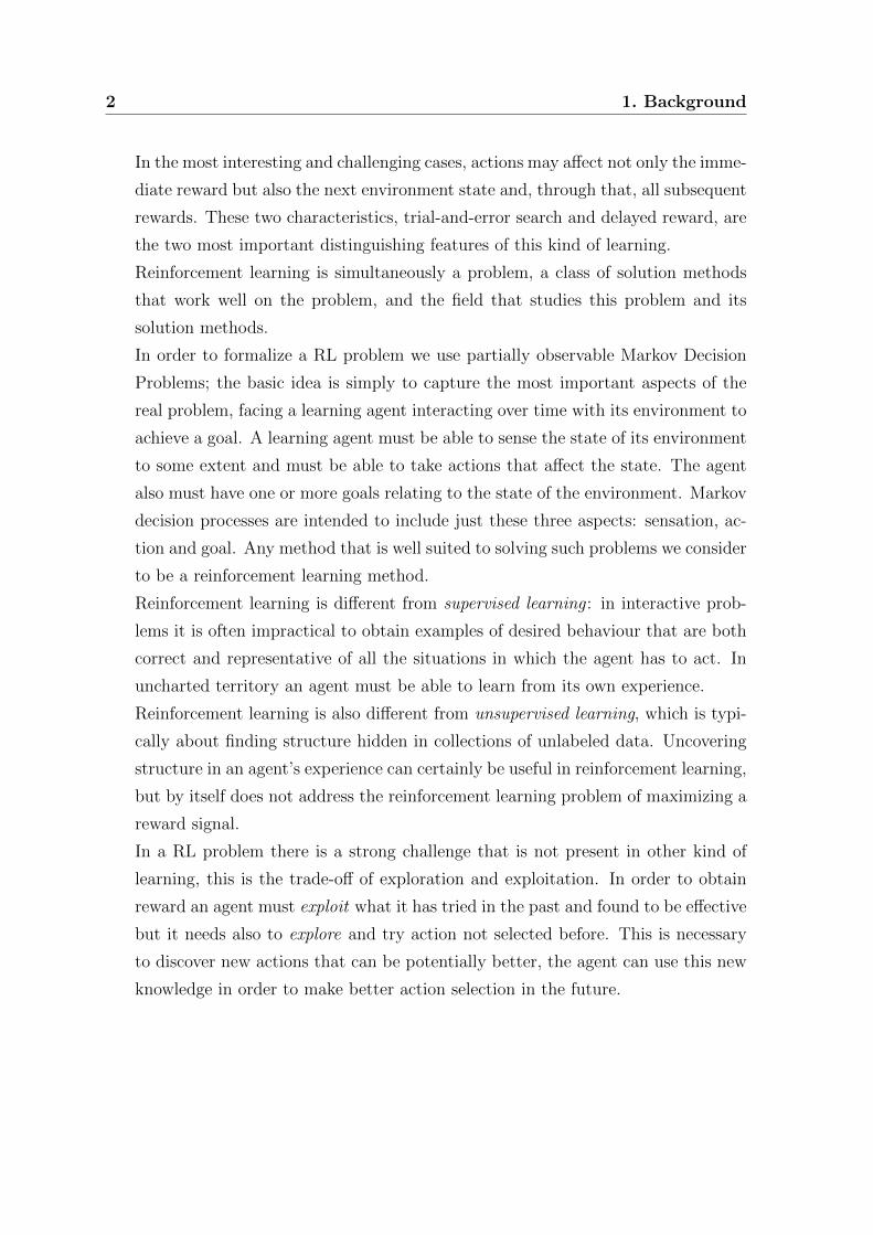
In the most interesting and challenging cases, actions may affect not only the imme-
diate reward but also the next environment state and, through that, all subsequent
rewards. These two characteristics, trial-and-error search and delayed reward, are
the two most important distinguishing features of this kind of learning.
Reinforcement learning is simultaneously a problem, a class of solution methods
that work well on the problem, and the field that studies this problem and its
solution methods.
In order to formalize a RL problem we use partially observable Markov Decision
Problems; the basic idea is simply to capture the most important aspects of the
real problem, facing a learning agent interacting over time with its environment to
achieve a goal. A learning agent must be able to sense the state of its environment
to some extent and must be able to take actions that affect the state. The agent
also must have one or more goals relating to the state of the environment. Markov
decision processes are intended to include just these three aspects: sensation, ac-
tion and goal. Any method that is well suited to solving such problems we consider
to be a reinforcement learning method.
Reinforcement learning is different from supervised learning : in interactive prob-
lems it is often impractical to obtain examples of desired behaviour that are both
correct and representative of all the situations in which the agent has to act. In
uncharted territory an agent must be able to learn from its own experience.
Reinforcement learning is also different from unsupervised learning, which is typi-
cally about finding structure hidden in collections of unlabeled data. Uncovering
structure in an agent’s experience can certainly be useful in reinforcement learning,
but by itself does not address the reinforcement learning problem of maximizing a
reward signal.
In a RL problem there is a strong challenge that is not present in other kind of
learning, this is the trade-off of exploration and exploitation. In order to obtain
reward an agent must exploit what it has tried in the past and found to be effective
but it needs also to explore and try action not selected before. This is necessary
to discover new actions that can be potentially better, the agent can use this new
knowledge in order to make better action selection in the future.
1.1 Reinforcement Learning 3
AgentEnvironment
Observation
Action
Reward
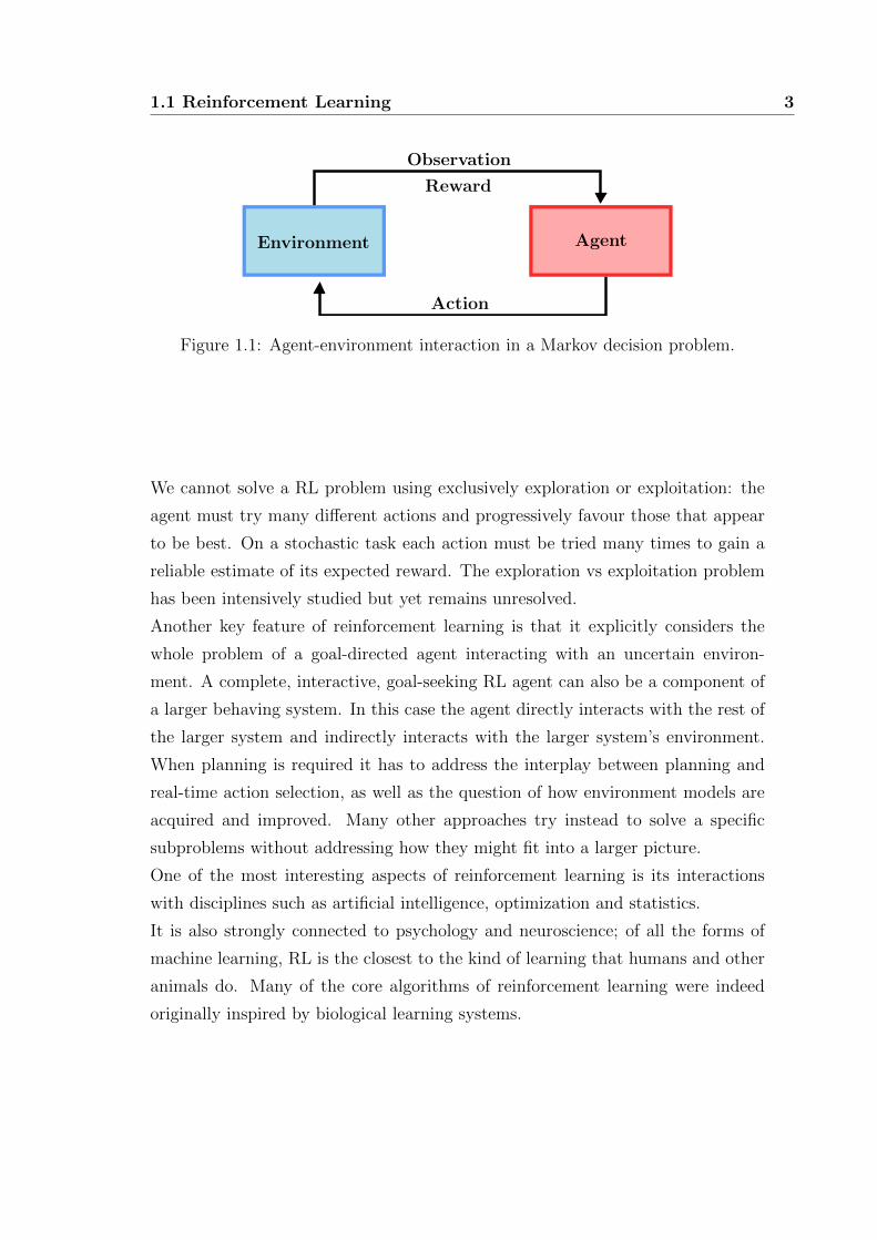
Figure 1.1: Agent-environment interaction in a Markov decision problem.
We cannot solve a RL problem using exclusively exploration or exploitation: the
agent must try many different actions and progressively favour those that appear
to be best. On a stochastic task each action must be tried many times to gain a
reliable estimate of its expected reward. The exploration vs exploitation problem
has been intensively studied but yet remains unresolved.
Another key feature of reinforcement learning is that it explicitly considers the
whole problem of a goal-directed agent interacting with an uncertain environ-
ment. A complete, interactive, goal-seeking RL agent can also be a component of
a larger behaving system. In this case the agent directly interacts with the rest of
the larger system and indirectly interacts with the larger system’s environment.
When planning is required it has to address the interplay between planning and
real-time action selection, as well as the question of how environment models are
acquired and improved. Many other approaches try instead to solve a specific
subproblems without addressing how they might fit into a larger picture.
One of the most interesting aspects of reinforcement learning is its interactions
with disciplines such as artificial intelligence, optimization and statistics.
It is also strongly connected to psychology and neuroscience; of all the forms of
machine learning, RL is the closest to the kind of learning that humans and other
animals do. Many of the core algorithms of reinforcement learning were indeed
originally inspired by biological learning systems.
4 1. Background
1.2 Finite MDP
Markov Decision Problems (MDP) are a classical formalization of sequential
decision making where actions influence not just immediate rewards, but also sub-
sequent states and through those future rewards. In order to solve a MDP the need
to tradeoff immediate and delayed reward must be considered. In this formaliza-
tion the learner that makes decisions is called agent while the thing it interacts
with, comprising everything outside the agent, is called the environment.
Agent and environment interact continually at discrete time steps t = 0, 1, 2, etc.
At each time step t the agent receive a representation of the state st ∈ S and,
observing that, it select an action at ∈ A(st) or simply at ∈ A. At the following
time step t + 1 the agent receive the representation of state st+1 and a numerical
reward rt+1 ∈ R ⊂ R.
In a finite MDP the sets A, S and R have a finite number of elements. In this
scenario random variables Rt and St have a well defined discrete probability dis-
tributions dependent only on the preceding state and action. We can then define
the probability of being in a state s′ ∈ St with reward r ∈ Rt after selecting action
a in state s at time step t− 1:
p(s′, r|s, a) = P{St = s′, Rt = r|St−1 = s, At−1 = a}
for all s, s′ ∈ S, r ∈ R, a ∈ A(s). The function p is called the dynamics of
an MDP as it completely characterizes the environment’s dynamics. From this
follows that the probability of each possible value for St and Rt depends only
on the immediately preceding state and action St−1 and At−1 and not on earlier
states and actions. The state must include information about all aspects of the
past interaction between agent and environment that make a difference for the
future.
The agent-environment interaction is illustrated in Figure 1.1. From the dynamics
can be derived other useful probabilities and one can compute anything else one
might want to know about the environment.
MDPs are a very general framework: actions can be low-level controls or high-level
decisions, time steps can refer to arbitrary successive stages of decision making.

1.3 Reward 5
Similarly states can be completely determined by low-level sensations or they can
be more high-level and abstract. In general, actions can be any decisions we want
to learn how to make and the states can be anything we can know that might be
useful in making them.
In order to solve a particular task we must define the agent-environment boundary,
this change is based on the level of abstraction we need. In a complicated task many
agent may be operating at once, each with its own boundary. In general, anything
that cannot be changed arbitrarily by the agent is considered to be outside of it and
thus part of its environment. We do not assume that the environment is completely
unknown to the agent but reward computation is considered to be external to the
agent because it defines the task and thus must be beyond its ability to change
arbitrarily. The agent-environment boundary thus represents the limit of what the
agent can completely control, not of what it knows. It is determined once one has
selected particular states, actions, and rewards, and thus has identified a specific
task of interest.
With MDPs any problem of learning goal-directed behaviour can be reduced to
three signals: actions, states and rewards; it may not be sufficient to represent
all decision-learning problems usefully but it has proved to be widely useful and
applicable.
1.3 Reward
The goal of an agent is formalized using a signal called reward, this is simply a
number Rt ∈ R passed by the environment at each time step. Every RL agent tries
to maximize the total reward obtained during its lifetime, this means maximizing
not immediate reward but cumulative reward in the long run. Though it seems
limited it has proved to be flexible and widely applicable, it is used to define what
are the bad and good events for the agent. It can be thought as analogous to the
experience of pleasure and pain. In the case of a cleaning robot, for example, a
possible reward system could be -1 when it bumps into things or when somebody
yells at it, +1 when it cleans a small area and 0 otherwise.

6 1. Background
Rewards must be provided in such a way that in maximizing them the agent
will also achieve established goals. A common mistake is to give a reward upon
reaching subgoals, in this case the agent might find a way to achieve them without
achieving the real goal. Rewards are used to communicate what the agent must
achieve and not how to obtain it.
1.4 Episode
Previously we have said that an RL agent seeks to maximize the cumulative
reward it receive in the long run, more specifically it needs to maximize the ex-
pected return, where the return is a specific function of a reward sequence. In
general the most simple return is the sum of rewards between two time steps, a
start step and a final step. We define the expected return as:
Gt =∑T
k=0Rt+k+1
This approach can be used when the interaction between agent and environment
can be broken naturally into independent subsequences called episodes. Each
episode ends in a special state called terminal state, it is followed by a reset to
a standard starting state or to a sample from a standard distribution of starting
states. In case of a board game like chess, for example, the terminal state could be
reached when a match ends. Tasks with episodes of this kind are called episodic
tasks. In many cases the agent-environment interaction does not break naturally
into identifiable episodes, but goes on continually without limit, we call these con-
tinuing tasks. In continuing tasks the definition of expected return is problematic
because the final step could be T = ∞, in order to obviate to this problem we
introduce the concept of discounting. In this case the agent selects an action and
seeks to maximize the expected discounted return that is defined as:
Gt =∑T
k=0 γkRt+k+1
where γ ∈ [0, 1] is called the discount rate. If γ < 1 the infinite sum in the defini-
tion of Gt has a finite value as long as the reward sequence is bounded.

1.5 Policy 7
The discount rate is used to balance the importance that the agent gives to imme-
diate and future rewards. If γ is close to 0 the agent prefers immediate rewards, in
general acting to maximize immediate reward can reduce access to future rewards
so that the return is reduced. If γ is close to 1 the the agent takes future rewards
into account more strongly and it becomes more farsighted.
If we define Gt+1+T = 0, thus imposing a null expected return after T timesteps,
then for t < T we can relate returns at successive time steps as:
Gt = Rt+1 + γ(Rt+2 + γRt+3 + ...) = Rt+1 + γGt+1
This is a very important relation because it allows to express the discounted ex-
pected return as the sum of the immediate reward and the discounted expected
return at the next time step.
1.5 Policy
In order to define the agent’s way of behaving we introduce the concept of
policy. It can be thought as a mapping from perceived states to actions to be
taken when in those states; it corresponds to what in psychology would be called
a set of stimulus-response rules or associations. In some cases it could be a simple
function or lookup table, in many other cases it is a complex and expensive func-
tion. It alone determines the agent’s behaviour and in general may be stochastic,
specifying probabilities for each action.
Formally, a policy is a mapping from states to probabilities of selecting each pos-
sible action. If the agent is following policy π at time step t then:
π(a|s) = P{At = a|St = s}
for all a ∈ A(s) and s ∈ S; π defines a probability distribution over a ∈ A(s)
for each s ∈ S. Reinforcement learning methods specify how the agent’s policy is
changed as a result of its experience.
8 1. Background
The reward signal discussed before is mainly used to alter the policy, if an action
selection is followed by a low reward then the policy is modified in order to decrease
the probability of performing the same action selection again in the future. In
general reward signals are difficult to predict and may be stochastic functions of
the state of the environment and the actions taken.
1.6 Value function
The reward signal discussed before indicates what is the best immediate return,
in order to represent what is good in the long run we define the value function.
The value of a state is the amount of reward that the agent expects to accumulate
over time starting from that state. The agent must seek actions that lead to
states of higher values rather than highest rewards because these actions obtain
the greatest amount of reward for us over the long run. For example, a state
might always yield a low immediate reward but still have a high value because it
is regularly followed by other states that yield high rewards, the reverse could also
be true. While rewards are somewhat like pleasure and pain, values correspond to
a more farsighted judgement of how pleased or displeased it is for the agent to be
in a given state.
Rewards are given directly by the environment while values must be continuously
re-estimated from the observations that the agent makes over its lifetime, this
makes values estimation much harder than reward evaluation. The most important
component of all RL algorithm is typically a method for efficiently estimating
values.
Value functions are denoted as Vπ(s) and are defined with respect to particular
policy π with a state s as input. Formally it is defined as:
Vπ(s) = Eπ[Gt|St = s] = Eπ[∑∞
k=0 γkRt+k+1|St = s]
for all s ∈ S where Eπ denotes the expected value of a random variable given that
the agent follows policy π, t is any time step. The value of a terminal state is 0,
this function is called the state-value function for policy π.
1.6 Value function 9
As discussed before a policy is continually modified considering the agent’s previous
experiences. In order to make a change we must be able to compare two policies
and decide which is the best. A policy π is defined to be better or equal to a policy
π′ if and only if Vπ(s) ≥ Vπ′(s) for all s ∈ S. There is always at least a policy
equal or better to all the other policies and is called the optimal policy, we denote
these by π∗. The value function is a good method that can be used to measure
the quality of a policy.
We can define also a value function denoting the expected return starting from s,
taking the action a, and thereafter following policy π:
Qπ(s, a) = Eπ[Gt|St = s, At = a] = Eπ[∑∞
k=0 γkRt+k+1|St = s, At = a]
for all s ∈ S and a ∈ A(s), this function is called the action-value function for
policy π. The difference between action-value and state-value is the advantage
function and it is expressed as:
Aπ(s, a) = Qπ(s, a)− Vπ(s)
An agent can follow policy π and maintain an average, for each state encountered,
of the actual returns that have followed that state. The average will than converge
to the state’s value Vπ(s), as the number of times that state is encountered ap-
proaches infinity. If the agent keeps averages for each action taken in each state,
then these will similarly converge to the action values Qπ(s, a). These methods
are called Monte Carlo.
The fundamental relationships used throughout reinforcement learning and dy-
namic programming are Bellman equations, they express a relationship between
the value of a state and the values of its successor states. They are defined as
follows, for all a ∈ A and s ∈ S:
Vπ(s) =∑a
π(a|s)∑s′,r
p(s′, r|s, a)[r + γVπ(s′)]
Qπ(s, a) =∑s′,r
p(s′, r|s, a)[r + γ∑a′π(a′, s′)Qπ(s′, a′)]
Starting from state s the agent could take any of some set of actions based on its
policy π. From each of these the environment could respond with one of several

10 1. Background
next states s′ along with a reward r, depending on its dynamics. The Bellman
equations averages over all the possibilities, weighting each by its probability of
occurring. It states that the value of the start state must equal the (discounted)
value of the expected next state, plus the reward expected along the way.
All optimal policies share the same state-value functions V∗(s) and Q∗(s, a) called
optimal state-value function and optimal action-value function respectively. These
functions are defined as:
V∗(s) = maxπ
Vπ(s)
Q∗(s, a) = maxπ
Qπ(s, a)
for all s ∈ S and a ∈ A(s). V∗(s) and Q∗(s, a) must satisfy the self-consistency
conditions given by the Bellman equations for state values. The Bellman equation
for V∗, called Bellman optimality equation, expresses the fact that the value of a
state under an optimal policy must equal the expected return for the best action
from that state and is defined as follows:
V∗(s) = maxa
∑s′,r
p(s′, r|s, a)[r + γV∗(s′)]
We can also define the Bellman optimality equation for Q∗ as:
Q∗(s, a) =∑s′,r
p(s′, r|s, a)[r + γmaxa′
Q∗(s′, a′)]
Finding V∗ allows to easily determine an optimal policy, any policy that is greedy
with respect to the optimal evaluation function V∗ is an optimal policy. Explicitly
solving the Bellman optimality equation in order to obtain an optimal state-value
function however is rarely possible. This solution is similar to an exhaustive search
and relies on at least three assumptions that are rarely true in practice:
• Knowledge of the environment’s dynamics
• Enough computational resources to complete the computation of the solution
• Markov property

1.7 Model 11
Figure 1.2: Classic board games Go (left) and Backgammon (right).
In reinforcement learning we typically have to settle for approximate solutions; in
many problems there may be many states that the agent faces with such a low
probability, that selecting suboptimal actions for them has little impact on the
amount of reward the agent receive. It is then possible to approximate optimal
policies in ways that put more effort into learning to make good decisions for
frequently encountered states, at the expense of less effort for infrequently encoun-
tered states. This is one central property that distinguish RL from other methods
to approximately solving MDPs.
1.7 Model
In some cases a model of the environment can be useful to improve learning
of an agent, it is basically something that emulates the environment and allows
inferences to be made about its future behaviour. Given a state and action the
model can predict the resulting state and reward. A model is used for planning:
the agent decides a course of actions considering possible future situations before
they are actually experienced.
Reinforcement learning algorithms that use a model for planning are called model-
based methods while less complex algorithms that learn explicitly by trial-and-error
are called model-free methods. There are also hybrid approaches where RL systems
simultaneously learn by trial-and-error, learn a model of the environment and use
the model for planning. Modern reinforcement learning spans the spectrum from
low-level, trial-and-error learning to high-level, deliberative planning.

12 1. Background
1.8 Applications
Reinforcement learning has a wide range of applications, games are excellent
testbeds for measuring an algorithm’s performances. Progress has been made
on perfect information games like Backgammon [12] and Go [13] as well as im-
perfect information games like Heads-up Limit Hold’em Poker [6]. Video games
represents another great challenge for RL algorithms, Atari 2600 [10] is the most
famous testbed but progress has been made on Doom [14], Starcraft [15] and many
other games.
Another classical area for reinforcement learning is robotics, common tasks include
object localization and manipulation, visual tracking as well as navigation.
NLP (Natural Language Processing) presents many issues that can be addressed
with RL algorithm; these are, for example, information extraction and retrieval,
summarization, sentiment analysis and many others. A lot of research has been
made in different NLP areas such as machine translation, dialogue systems and
text generation.
Reinforcement learning would be also an important ingredient in Computer Vision
in tasks like object segmentation, object dynamics learning and haptic property
estimation, object recognition or categorization, grasp planning and manipulation
skill learning.
Other areas which can be influenced by RL are business management, health-
care, finance, education, industry and even electricity management and intelligent
transportation systems.

Chapter 2
RL algorithms
In this chapter we discuss the main approaches to reinforcement learning, in
particular we will see the most important algorithms proposed in recent years such
as DQN [3], A3C [9] and ACER [8].
2.1 Dynamic programming
Dynamic programming (DP) are a collection of algorithms that can be used to
compute optimal policies given a perfect model of the environment as a Markov de-
cision process. They are of limited utility because the model is often unknown and
they are computationally expensive but they remain theoretically useful. While
DP ideas can be applied to problems with continuous state and action spaces ex-
act solutions are possible only in special cases. In order to obtain approximate
solutions for tasks with continuous states and actions, the state and action spaces
can be quantized and then finite-state DP methods are applied. Knowing environ-
ment’s dynamics we can start from Bellman equation for Vπ and define an iterative
method for computing the state-value function for an arbitrary policy π, we call
this problem policy evaluation.
In order to evaluate the state-value function an initial approximation V0 for all
states is chosen arbitrary except that the terminal state, if any, must be given
value 0.
13

14 2. RL algorithms
Each successive approximation is obtained using the following update rule:
Vk+1(s) =∑a
π(a|s)∑s′,r
p(s′, r|s, a)[r + γVk(s′)]
for all s ∈ S. The algorithm applies iteratively the update rule until a fixed point
is reached. The existence and uniqueness of Vπ are guaranteed as long as either
γ < 1 or eventual termination is guaranteed from all states under the policy π;
these conditions ensure also that the sequence in general converges as k → ∞.
Policy evaluation can be used to find better policies, this process is called policy
improvement. Suppose that Vπ(s) has been computed using policy evaluation and
let π and π′ be any pair of deterministic policies such that:
Qπ(s, π′(s)) ≥ Vπ(s)
for all s ∈ S, then π′ must be as good as, or even better than, π. This result can
be used to understand if changing an action selection in a state for current policy
leads to an improvement. As a result Vπ′(s) ≥ Vπ(s) for all s ∈ S, if the first
inequality is strict at any state then the second inequality must be strict.
Using previous consideration a new policy π′ can be obtained from π using the
following update rule.
π′(s) = argmaxa
Qπ(s, a) = argmaxa
∑s′,r
p(s′, r|s, a)[r + γVπ(s′)]
Policy improvement thus result in a strictly better policy except when the original
policy is already optimal; these ideas are valid on both deterministic and stochastic
policies. Using policy improvement we can determine a policy π′, from this a new
state-value function Vπ′ can be derived using policy evaluation. The value function
can be employed to obtain a better policy π′′, this process is called policy iteration.
In Finite MDPs this process converges to an optimal policy and optimal value
function in a finite number of iterations. Below is illustrated the whole sequence
whereE−−−−−→ denotes evaluation and
I−−−−→ denotes improvement.
π0E−−−−−→ Vπ0
I−−−−→ π1E−−−−−→ ...
I−−−−→ π∗E−−−−−→ V∗

2.2 Monte Carlo 15
The general idea behind policy iteration is called Generalized Policy Iteration
(GPI); in GPI there are two interacting processes, one process takes the policy
and performs some form of policy evaluation, changing the value function to be
more like the true one for the policy. The other process takes the value function and
performs some form of policy improvement, changing the policy to make it better,
assuming that the value function is its value function. This pair of processes work
together to find an optimal solution. In some cases, like those discussed before,
GPI can be proved to converge, in other cases convergence has not been proved.
An interesting property of DP methods is that they update estimates of the values
of states based on estimates of the values of successor states. They thus update
estimates on the basis of other estimates, this general idea is called bootstrapping
and is used also in Temporal-Difference Learning which we will discuss later.
2.2 Monte Carlo
Monte Carlo methods do not assume complete knowledge of the environment
and learning is made from experience without requiring prior knowledge of the
environment’s dynamics. These methods assume that experience is divided into
episodes, and that all episodes eventually terminate no matter what actions are
selected. The reason is that the episode has to terminate before any reward cal-
culation, policy updates are done after every episode. The idea behind MC is
simple: the value is the mean return of all sample trajectories for each state, sim-
ilar to Dynamic Programming there are two phases: policy evaluation and policy
improvement.
These methods needs to learn from complete episodes to compute the expected
discounted reward Gt =∑T−t−1
k=0 γkRt+k+1, the empirical mean return for state s
is:
Vπ(s) = E[Gt|St = s] = 1N
N∑i=1
Git,s
where Git,s is the expected discounted reward for state s at time step t and episode
i, N is the number of episodes.

16 2. RL algorithms
We may average returns for every time s is visited in an episode (“every-visit”),
or average returns only for first time s is visited in an episode (“first-visit”). This
way of approximation can be easily extended to action-value functions by counting
(s, a) pairs:
Qπ(s, a) = E[Gt|St = s, At = a] = 1N
N∑i=1
Git,s,a
where Git,s,a is the expected discounted reward for state s and action a at time
step t and episode i. Normally it is convenient to convert the mean return into
an incremental update so that the mean can be updated with each episode and
we can understand the progress made with each episode. In order to learn the
optimal policy by Monte Carlo methods, a procedure similar to policy iteration
from previous section can be used:
• Improve the policy greedily with respect to the current action-value function
π(s) = argmaxa
Q(s, a).
• Generate a new episode with the new policy π.
• Estimate Q using the new episode as we have discussed earlier.
A policy obtained with the discussed method will always favour certain actions if
most of them are not explored properly. There are two possible solution to this
problem: exploring starts and ε-soft. In Monte Carlo methods with exploring starts
all the state-action pairs have non-zero probability of being the starting pair. This
will ensure that each episode which is played will take the agent to new states and
hence, there is more exploration of the environment. Exploring starts is not usable
in environment where there is a single start point, in this cases ε-soft methods can
be used. With this strategy all actions are tried with non-zero probability, with
probability 1 − ε the algorithm chooses the action which maximises the action
value function and with probability ε it selects an action at random.
One important distinction in RL is on-policy vs off-policy. In on-policy methods
the agent tries always to explore and attempts to find the best policy that still
explores.

2.3 Temporal-Difference 17
In off-policy methods the agent explores but learns a deterministic optimal policy
that may be unrelated to the policy followed. More formally off-policy prediction
refers to learning the value function of a target policy from data generated by a
different behaviour policy.
Off-policy Monte Carlo methods are a family of interesting methods, they are
based on some form of importance sampling ; this consists on weighting returns by
the ratio of the probabilities of taking the observed actions under the two policies,
thereby transforming their expectations from the behaviour policy to the target
policy.
Importance sampling can be ordinary and uses a simple average of the weighted
returns, weighted importance sampling instead uses a weighted average. Ordinary
importance sampling produces unbiased estimates but has larger, possibly infinite
variance, whereas weighted importance sampling always has finite variance and
is preferred in practice. These methods are conceptually simple but are still a
subject of ongoing research.
Monte Carlo and DP methods differ in two major ways. MC algorithms operate
on sample experience and thus can be used for direct learning without a model.
Secondly they do not bootstrap therefore they do not update their value estimates
on the basis of other value estimates.
2.3 Temporal-Difference
Temporal-Difference learning is a central and novel approach in RL and is a
combination of Monte Carlo and Dynamic Programming ideas. Like MC algo-
rithms they can learn directly from raw experience without a model of the envi-
ronment’s dynamics, and like DP algorithms they update estimates based in part
on other learned estimates, without waiting for a final outcome (bootstrap).
TD learning use some variation of generalized policy iteration (GPI); in particular
policy evaluation, or TD prediction, works like in Monte Carlo methods. Starting
from some experiences collected from policy π both methods update their estimate
of Vπ for the non-terminal states St occurring in those experiences.

18 2. RL algorithms
Monte Carlo methods must wait until the return Gt is known, then use that return
as a target for V (St). They must wait until the end of the episode to determine
the increment to V (St).
A simple every-visit Monte Carlo method suitable for non-stationary environments
can be written as:
V (St)← V (St) + α[Gt − V (St)]
where Gt is the actual return following time t, and α is a constant step-size pa-
rameter. Compared to MC methods TD algorithms need to wait only until the
next time step. At time t + 1 they immediately form a target and make a useful
update using the observed reward Rt+1 and the estimate V (St+1). The general
rule for update of V (St) is:
V (St)← V (St) + α[Rt+1 + γV (St+1)− V (St)]
Whereas target for Monte Carlo update is Gt in TD algorithms the target is
Rt+1 + γV (St+1), this method is called TD(0) or one-step TD and it is a special
case of more complex algorithms like TD(γ) and n-step TD. As said before TD
methods use bootstrapping and TD(0) is a perfect example: the update is based
in part on an existing estimate that is V (St+1).
The quantity in brackets in the update rule measures the difference between the
estimated value of St and the better estimate Rt+1+γV (St+1), it is called TD-error
and is a very common concept in reinforcement learning. It is commonly denoted
as δt and it is defined as:
δt = Rt+1 + γV (St+1)− V (St)
TD methods have an advantage over DP methods in that they do not require
a model of the environment and compared to Monte Carlo they don’t need to
wait until the end of an episode but only one step. This conditions make TD
algorithms usable in a larger range of applications. Moreover, tuning opportunely
the α parameter, for any policy π, TD(0) has been proven to converge to Vπ though
no one has been able to prove mathematically that TD learning methods converge
faster than MC ones.

2.3 Temporal-Difference 19
We have discussed of policy evaluation for TD learning, as before we follow the
pattern of GPI and present two major approach for policy improvement or TD
control : Sarsa and Q-learning.
2.3.1 Sarsa
In order to define this TD control algorithm we must define an update rule for
estimating action-value Qπ(s, a) for the current behavior policy π and for all states
s and actions a. This can be done using essentially the same method described
above for learning state-value function:
Q(St, At)← Q(St, At) + α[Rt+1 + γQ(St+1, At+1)−Q(St, At)]
Sarsa is an on-policy method because it estimates the value of a policy assuming the
current policy continues to be followed. As in all on-policy methods we continually
estimate Qπ for the behaviour policy π and, at the same time, change the policy
toward greediness with respect to Qπ. This update is done after every transition
from a non-terminal state St, if St+1 is terminal then Q(St+1, At+1) is defined as
zero. The algorithm proceeds as follows:
1. At time step t from state St select an action At accordingly to the current
policy derived from Q, in this case ε-soft or ε-greedy are commonly applied.
2. Observe reward Rt+1 and get the new state St+1.
3. Pick the next action At+1 from state St+1 in the same way as in (1).
4. Use the update rule in order to better approximate Q(St, At).
5. t = t+ 1 and repeat from (1).
The convergence of the Sarsa algorithm depend on the nature of the policy’s de-
pendence on Q, this can be changed for example using ε-greedy or ε-soft strategies.
The method converges to an optimal policy and action-value function as long as all
state-action pairs are visited an infinite number of times and the policy converges
in the limit to the greedy policy.

20 2. RL algorithms
2.3.2 Q-learning
The development of an off-policy TD control algorithm known as Q-learning
was a big breakout in the early days of reinforcement learning. In this case the
update rule used to approximate the action-value function is:
Q(St, At)← Q(St, At) + α[Rt+1 + γmaxaQ(St+1, a)−Q(St, At)]
In Q-learning the learned action-value function directly approximates Q∗ indepen-
dent of the policy being followed. The algorithm proceeds as follows:
1. At time step t from state St select an action At accordingly to Q, in this case
ε-soft or ε-greedy are commonly applied.
2. Observe reward Rt+1 and get the new state St+1.
3. Use the update rule in order to better approximate Q(St, At).
4. t = t+ 1 and repeat from (1).
The first two steps are same as in Sarsa. In step (3) Q-learning does not follow
the current policy to pick the second action but rather estimate Q∗ out of the
best Q values independently of the current policy. The analysis of Q-learning is
simpler, the policy still has an effect in that it determines which state-action pairs
are visited and updated. Q-learning has been shown to converge to Q∗ under the
assumption that all state-action pairs are visited and continue to be updated. In
order to ensure convergence determined conditions on the sequence of step-size
parameters must be observed.
2.3.3 DQN
Theoretically we can memorize action-value Q(s, a) for all state-action pairs in
Q-learning but for realistic problems this is not possible due to the large state and
action spaces. In order to approximate Q values, a function is used instead: this is
called function approximator. For example if a function with parameter θ is used
to approximate Q-values, we can label it as Q(s, a, θ).

2.3 Temporal-Difference 21
Input
84x84x4
Conv layer
+ReLU
32@8x8x464@4x4x2
Conv layer
+ReLU
64@3x3x1
Conv layer
+ReLU FC
layer
Output
51218
Figure 2.1: DQN neural network architecture.
Q-learning may suffer from instability and divergence when combined with a
non-linear Q-value function approximation and bootstrapping. In order to over-
come this problem another algorithm has been introduced and is called Deep Q-
Network [4] [3]. This method combines Q-learning with a deep neural network
that is used as function approximator.
Deep neural networks are machine learning algorithms that use a cascade of multi-
ple layers of non-linear processing units for feature extraction and transformation.
Each successive layer uses the output from the previous layer as input; they learn
in supervised or unsupervised mode. Each level learns to transform its input data
into a slightly more abstract and composite representation. They can be trained
to solve many different tasks, from image recognition to automatic speech recog-
nition. Deep neural networks are used as a function approximator in DQN and in
many subsequent works.
As we have seen before training a deep neural network combined with Q-learning
is not guaranteed to converge and is in general unstable. DQN aims to greatly
improve and stabilize the training process introducing two major innovations:
• Experience Replay
Replaying consecutive samples with Q-learning can be inefficient and updates
suffer of high variance. With this technique all the episode steps are stored
in one replay memory that has a size of one million elements. During Q-
learning updates, 32 samples are drawn at random from the replay memory
and thus one sample could be used multiple times. This forms an input
dataset which is stable enough for training.

22 2. RL algorithms
The idea behind Experience Replay is not new [7] but, combined with Q-
learning, improves data efficiency, removes correlations in the observation
sequences and smooths over changes in the data distribution.
• Periodically Updated Target
In TD error calculation, target function is changed frequently with DNN
and unstable target function makes training difficult. Using this technique
Q-values are optimized towards target values that are only periodically up-
dated. The Q network is cloned and kept frozen as the optimization target
every C steps, where C is an hyperparameter. This modification makes the
training more stable as it overcomes the short-term oscillations.
Other two innovation introduced in this work are Frame Skipping and Reward
Clipping. Using Frame Skipping DQN calculates Q values every m frames (typi-
cally m = 4): the agent doesn’t need to calculate Q values every frame and people
don’t take actions so frequently. Once an action selection is made that action
is executed for 4 subsequent frame, this reduces computational cost and gathers
experiences more quickly.
In different problems rewards can vary from high points for important achieve-
ments to low points for less important ones. This difference can make training
unstable, using Clipping Rewards scores are clipped and all positive rewards are
set to +1 and all negative rewards are set to -1, this can help stabilizing training.
In the original works DQN has been tested on the Atari 2600 emulator [10] which
we will present in the next chapter. Atari frames are 210x160 pixel images with a
128 color palette, an input so large can be computationally demanding so images
are preprocessed by first converting their RGB representation to gray-scale and
down-sampling it to a 84x84 image that roughly captures the playing area.
In order to encode a single frame is taken the maximum value for each pixel color
value over current and previous frame. This is necessary to remove flickering that
is present in games where some objects appear only in even frames while other
objects appear only in odd frames. The neural network input are the last 4 frames
that are preprocessed and stacked, the input to the neural network consists in an
84x84x4 image that is fed to a dedicated layer.

2.4 Policy gradient 23
The network architecture is reported in Figure 2.1, the first hidden layer is a con-
volutional layer of 32 8x8 filters with stride 4 followed by a rectifier nonlinearity.
The second hidden layer is a convolutional layer of 64 4x4 filters with stride 2 again
followed by a rectifier nonlinearity. After that there is a third convolutional layer
of 64 3x3 filters with stride 1 followed by a rectifier. The final hidden layer is fully-
connected and consists of 512 rectifier units. The output layer is fully-connected
with a single output for every possible action.
The outputs correspond to the predicted Q-values of the action for the input state.
The main advantage of this type of architecture is the ability to compute Q-values
for all possible actions in a given state with only a single forward pass through the
network. There are many extensions of DQN that improve the original design, such
as Double DQN [16], Dueling DQN [17] and Prioritized Experience Replay [18].
2.4 Policy gradient
All the methods we have discussed before try to learn the state-action value
function and then to select actions accordingly, Policy Gradient methods instead
learn the policy directly with a parameterized function respect to θ: π(a|s, θ). In
order to approximate the expected return we must define a reward function J(·),the value of the reward function depends on policy π and then various algorithms
can be applied to optimize θ for the best reward. The reward function in discrete
spaces is defined as:
J(θ) = Vπθ(S1)
where S1 is the initial state. For continuous spaces the function is defined as:
J(θ) =∑s∈S
dπθ(s)Vπθ(s) =∑s∈S
(dπθ(s)∑a∈A
πθ(a|s, θ)Qπ(s, a))
where dπθ = limt→∞ P (st = s|s0, πθ) is the probability of reaching state st when
starting from s0 and following policy πθ. Policy-based methods are more useful in
continuous space problems, in this tasks an algorithm has to estimate the value of
an infinite number of states and actions thus value-based approaches are way too

24 2. RL algorithms
computationally expensive. Using gradient ascent this methods move θ toward the
direction suggested by the gradient ∇θJ(θ) to find the best θ for πθ that produces
the highest return.
Computing the gradient ∇θJ(θ) is difficult because it depends on both the action
selection and the stationary distribution of states dπθ(·). The problem is that
gradient depends on two factors directly or indirectly dependent on πθ. Given
that the environment is generally unknown, it is difficult to estimate the effect on
the state distribution by a policy update. Luckily there is a theorem, called Policy
Gradient Theorem, that simplify the computation of the reward function that can
be rewritten as:
J(θ) ∝ Eπθ [∇θ ln π(a|s, θ)Qπθ(s, a)]
This is a theoretical foundation for various Policy Gradient algorithms, this allows
a policy gradient update with no bias but high variance. Various algorithms were
proposed to reduce the variance while keeping the bias unchanged.
2.4.1 REINFORCE
REINFORCE [19] is a combination of Policy Gradient and Monte Carlo, it
relies on an estimated return calculated using episode samples and it use that
return to update the policy parameter θ. In Policy Gradient methods ∇θJ(θ)
is calculated using expected return Qπθ(s, a), since Qπθ(s, a) = Eπθ [Gt|St, At] the
reward function can be rewritten as:
J(θ) ∝ Eπθ [∇θ ln π(a|s, θ)Gt]
As any other Monte Carlo method REINFORCE relies on a full trajectory, Gt is
indeed measured from real sample trajectories and used to update policy gradient
∇θJ(θ). A common and widely used variant of this algorithm uses the advantage
function Aπθ(s, a) = Qπθ(s, a) − Vπθ(s) in the gradient ascend update. In this
variant a baseline value (the state-value function) is subtracted from the return
Gt that represent the action-value function, this allows to reduce the variance of
the updates while keeping the bias unchanged. Thus the resulting training should
be more stable.

2.4 Policy gradient 25
2.4.2 A3C
Asynchronous Advantage Actor-Critic [9], or simply A3C, is a policy gradient
method with a special focus on parallel training and it is part of the actor-critic
algorithms family. In actor-critic methods there are two components: policy model
and value function. Unlike traditional policy gradient algorithms actor-critic tries
to learn both policy and value function, in fact it is useful to learn the value
function because it can be used to assist the policy update by reducing gradient
variance.
Actor-critic methods consist of two components, which may optionally share pa-
rameters:
• Critic
The value function, that depending on the algorithm can be Qw(s, a) or
Vw(s), is parameterized by w; the critic updates this parameter in order to
learn the function.
• Actor
Updates the policy parameters θ for πθ(a, s) in the direction suggested by
the critic.
This algorithm is designed to work well for parallel training; in A3C the critics
learn the value function while multiple actors are trained in parallel and get synced
with global parameters from time to time.
Using state-value function as an example, the loss function to be minimized for
value function approximation is the mean squared error Jv(w) = (Gt − Vw(s))2,
gradient descent can be applied to find the optimal w.
The value function is used as the baseline in the policy gradient update, gradients
with respect to w and θ are accumulated, this step can be considered as a paral-
lelized reformulation of minibatch-based stochastic gradient update. The values
of w and θ get corrected by a little bit in the direction of each training thread
independently, every environment gives a contribution to the final gradients.
A3C uses a deep neural network as a function approximator like DQN [4], the base

26 2. RL algorithms
network architectures are very similar except that in A3C there are two output
layers: one outputs a softmax policy and the other outputs the value of the current
state V (s).
2.4.3 TRPO
Both A3C and REINFORCE are on-policy methods because samples are col-
lected using the policy that is currently being optimized. Off-policy methods have
however several advantages: they don’t require full trajectories and can reuse any
past episodes for better sample efficiency, moreover they use a behaviour policy
different from the target policy, bringing better exploration. We define the be-
haviour policy, which is used to collect the samples, as µ(a|s).It’s not possible to use the same gradient as in on-policy methods because samples
were collected with a different policy respect to the current target. The gradient
is thus rewritten as:
∇θJ(θ) = Eµ[πθ(a|s)µθ(a|s)
Qπθ(s, a)∇θ ln πθ(a|s)]
where πθ(a|s)µθ(a|s)
is the importance weight, we write πθ(a|s) instead of π(a|s, θ) as a
more compact notation. This is an approximated gradient but it still guarantee
the policy improvement and eventually achieve the true local minimum.
Trust region policy optimization (TRPO) [20] is an algorithm that is available both
on-policy and off-policy, we will now see only the off-policy version. The idea be-
hind this method is that, in order to improve training stability, parameter updates
can’t change too much the policy in a single step. This method aims to maximize
the objective function J(θ) subject to a constraint (trust region constraint) which
enforces the distance between old and new policies to be within a parameter δ.
In order to measure the distance of the two policies is used KL-divergence that
measures how one probability distribution p diverges from a second expected prob-
ability distribution q and is defined as DKL(p‖q). DKL is asymmetric and achieves
the minimum zero when p(x) = q(x) everywhere.
If off-policy the objective function J(θ) measures the total advantage over the

2.4 Policy gradient 27
state visitation distribution and actions while following a different behaviour pol-
icy µ(a|s):
J(θ) = Es∼ρπθold ,a∼µ[πθ(a|s)µ(a|s) Aθold(s, a)]
where θold is the policy parameters before the update, ρπθold is the state visita-
tion distribution and Aθold(s, a) is the estimated advantage. The KL-divergence
constraint can be expressed as:
Es∼ρπθold [DKL(πθold(·, s)‖πθ(·, s))] ≤ δ
This can guarantee that old and new policies wouldn’t differ too much and it leads
to a monotonic policy improvement over time.
2.4.4 ACER
Actor-Critic with Experience Replay [8], or simply ACER, is an off-policy actor-
critic algorithm using Experience Replay. It is built on A3C and it is its off-policy
counterpart. This method uses the same network architecture as DQN [3] except
that there are two output layers: one outputs a softmax policy πθ(a|s) and the
other outputs the action values Qθv(s, a). ACER uses also the same pre-processing
technique as well as Frame Skipping and Reward Clipping.
It aims to greatly increase the sample efficiency and decrease the data correlation,
in order to control the stability of the off-policy estimator it uses three main
innovations:
• Retrace Q-value estimation
• Importance weights truncation with bias correction
• Efficient TRPO
Retrace
Retrace(λ) [21] is an off-policy multi-step value-based algorithm that guaran-
tees good data efficiency. It is part of the TD learning family and, similarly to

28 2. RL algorithms
Q-learning, it is sample efficient because it allows Experience Replay. It also en-
courages exploration because the sample collection follows a behaviour policy dif-
ferent from the target policy. Unlike Q-learning it uses multi-step, the advantages
are that rewards are propagated rapidly and bias introduced by bootstrapping is
reduced. Since it is a TD learning algorithm we can express TD error that, in this
case, is defined as:
δt = Rt+1 + γV (St+1)−Q(St, At)
The Q-values update is of the formQ(St, At)← Q(St, At)+αδt or simply ∆Q(St, At) =
αδt. We want to use δt to estimate Qπθ for an entire sample trajectory (it is a
multi-step algorithm) but this method is off-policy so we must use importance
sampling, the update becomes:
∆Q(St, At) = γt(∏
1≤τ≤t
π(Aτ |Sτ )µ(Aτ |Sτ ))δt
The problem with this update form is that the variance is not bounded, this
product thus can be very large and even explode. In order to overcome this
problem in Retrace the update expression is modified as:
∆Q(St, At) = γt(∏
1≤τ≤tλmin{1, π(Aτ |Sτ )
µ(Aτ |Sτ )})δt
This guarantees that variance is bounded and assures convergence for any pair
of policies π, µ. ACER uses Retrace to estimate Qπθ(St, At); given a trajectory
generated under the behaviour policy µ, the action-value approximation can be
expressed recursively as:
Qret(St, At) = Rt+1 + γmin{c, π(At|St)µ(At|St)}[Q
ret(St, At)−Qθv(St, At)] + γV (St+1)
where Qθv is the current estimate of Qπθ . In order to learn the critic Qθv ACER
uses Qret as a target in a mean squared error loss and update the action-value
function with the following gradient:
(Qret(St, At)−Qθv(St, At))∇θvQθv(St, At)
2.4 Policy gradient 29
Importance weight truncation
Truncating the importance weight reduces variance but introduces bias, in
order to overcome this problem ACER adds a correction term. The policy gradient
at time step t can thus be written as:
gacer = ρt(Qret(St, At)− Vθv(St))∇θ ln πθ(At|St)+
Ea∼π[max{0, ρt(a)−cρt(a)
}∇θ log πθ(a|St)(Qθv(St, a)− Vθv(St))]
where ρt = min{c, π(At|St)µ(At|St)}. The first term contains the clipped important weight,
the second term makes a correction to achieve unbiased estimation while reducing
update variance.
Efficient TRPO
ACER uses TRPO but, rather than measuring the KL divergence between
policies before and after one update, it maintains a running average of past policies
and forces the updated policy to not deviate far from this average. This is more
computationally efficient and allows a more stable learning process.
As A3C multiple threads collect samples in parallel but ACER also uses Experience
Replay, the default implementation define a buffer of 50000 elements for each
thread. This algorithm uses an hybrid approach: it makes one on-policy call that
works like A3C and a fixed number of off-policy calls, called replay ratio. With a
replay ratio of 4 ACER can obtain similar results respect to Prioritized DQN or
A3C but is more sample efficient; this means that the learning process is faster,
especially towards its on-policy counterpart A3C.
ACER has been used to tackle different problems, it performs well on a large variety
of tasks and it has been used to solve even hard exploration problems [22].

Chapter 3
ATARI
In order to measure performances of RL algorithms, various environments have
been used; the most famous problems that have been addressed in last years are
Atari 2600 games. Atari 2600 is a game console produced by Atari in 1977, it has
many available games, some very famous like Space Invaders or Pong. It repre-
sents a very challenging framework due to the variety of the playable games: it
goes from the more immediate Enduro to other games which requires some form
of planning like Gravitar.
Reinforcement learning problems can be divided in two categories: sparse rewards
problems and dense rewards problems. In dense rewards problems the agent can
easily obtain rewards even playing randomly, in these games learning is typically
faster and easier. On the contrary sparse rewards problems represents a very hard
challenge, in these tasks the agent is required to make a long sequence of proper
actions in order to obtain a single reward. Playing randomly in this case rarely
leads to a good result so it’s required to use efficiently the few positive experiences
made.
In 2013 DQN [4] first obtained very good results on these games, reaching super-
human skill levels in some of them; since then they have been used as the main
benchmark for the other proposed algorithms. The only one game in which DQN
obtained 0 points was Montezuma’s Revenge, it has become famous for its diffi-
culty and it is considered one of the hardest games of this suite.
30

3.1 Montezuma’s Revenge 31
Figure 3.1: Four Atari 2600 games, from left to right: Space Invaders, Pong,
Breakout and Pitfall.
In this work we use Montezuma’s Revenge as a testbed for various ideas. Per-
forming well in a notoriously difficult problem like this can be a significant result
though it doesn’t mean being effective in real world problems. In this chapter
we will present a description of MR dynamics and reward system, we will also
introduce OpenAI Gym [10], an interesting suite of RL tasks which has been used
in all experiments.
3.1 Montezuma’s Revenge
Montezuma’s Revenge, or simply MR, is a video game published in 1984 for
various platforms, in this title the player controls a character called Panama Joe.
The character can be moved from room to room in a labyrinthine underground
pyramid filled with enemies, obstacles, traps, and dangers. The game is very puni-
tive and the player has a significant number of ways to die; it has six lives and,
once the life counter goes to 0, the game ends. In MR there are 9 levels, they are
all similar but as the player advances some things change, for example the position
of items or the number of enemies and obstacles. A level is composed of 24 rooms
structured as a pyramid, the last two rooms are special and contains only coins:
they represent the treasures. The repetitive structure of the game implies that,
if an agent learn to solve an entire level, probably it can solve the entire game
supposing that it is able to generalize enough.

32 3. ATARI
Figure 3.2: The first room of Montezuma’s Revenge.
The problem is that most of the algorithms proposed are not able to pass even
the first room. In order to increase the score players must collect different objects;
there are keys, doors, coins, weapons and many others. It is possible to increase
the score even defeating enemies using weapons. The doors can only be opened us-
ing a compatible key, which then disappears. Players must thereby collect enough
of them in order to continue. Touching an enemy without a weapon results in a
life loss, in the first level once an enemy is touched it disappears. Every opponent
has its own look and behaviour, there are skulls that bounce or roll in the rooms,
lasers and bridges that periodically disappear and spiders that continuously move
horizontally. There are some dark rooms that become visible only if the player
has the torch object. In order to move across the game there are special objects
like ladders and ropes. The player can make different actions, it can move in the
eight main directions, it can do nothing or jump in any direction it wants.
Exiting the first room is already an achievement. Looking at Figure 3.2 the agent
must first obtain the key (100 points), then it must go downstairs and jump on
the yellow rope. After this it must go down a second time, avoid the skull and go
upstairs. Once it has taken the key it must come back to the starting point either
dying or following the reverse path, then it must touch one of the two doors (300
points each). The door on the left leads to a more difficult path full of lasers while
the other door leads to a longer but easier path.
Since DQN has been published many other algorithms were proposed, Table B

3.1 Montezuma’s Revenge 33
summarizes all major results on Montezuma’s Revenge. A3C and ACER perform
as badly as DQN; the first works that achieve a score similar to the average human
one on this game were two agent that combined intrinsic rewards with A3C and
DQN respectively [23], they are called DDQN-CTS and A3C-CTS. After those
another interesting work was DQN-PixelCNN [24] that further improved the pre-
vious algorithm without however increasing the score on MR. Other algorithms
that reached significant scores are The Reactor [25], Feature-EB [26], UBE [27],
Ape-X [28]. Another interesting work that uses intrinsic rewards is Curiosity-
driven learning [29] that obtains approximately 400 points (it exits the first room)
without using external rewards and more than 2500 points with a combination of
intrinsic and extrinsic rewards.
Recently two new algorithms have been released, they significantly outperform
the state of the art and are called RND [30] and Go-Explore [31]. Both of them
achieve a higher score than the average human using a novel and more difficult
testing procedure which we will see later. RND achieves 11347 points and uses
intrinsic rewards while Go-explore reaches 43763 points but it relies on strong
assumptions: for example the test they have made exploits the fact that the envi-
ronment is resettable to a particular state.
In the RND’s paper are also discussed results for PPO [32], another algorithm
recently presented that performs well on a large variety of tasks. The paper re-
ports a score for PPO of 2500 points; we will consider this and The Reactor as the
best results that don’t rely on strong assumptions on the environment and don’t
involve intrinsic rewards. These are indeed specifically thought for problems where
exploration is important.
Most of the methods proposed in the last years are trained for 50 million steps (or
200 million of frames with Frame Skipping of 4). We consider this as a standard,
this is the reason why we do not take into consideration algorithms like UBE and
Ape-X. In fact in the original paper of UBE, for example, the score reported is
achieved after 500 million of frames (with 200 million of frames it reaches only 500
points).

34 3. ATARI
3.2 OpenAI Gym
In order to provide a common test suite OpenAI, one of the most important
team in reinforcement learning development, developed Gym [10]. It is a set of
games and tasks specifically built for testing RL algorithms.
Gym is written in Python3 and provides different kind of tests and training envi-
ronments:
• Computation learning
• Simple toy text environment
• Atari 2600 games
• Classic control theory problems
• Continuous control tasks using 3D environment and a physics simulator
• Simulated goal-based tasks using 3D robots
RL has been massively developed only in the last couple of years thus initially
there wasn’t a common evaluation technique. In last years various methods were
proposed in order to accomplish this task, the most used are no-op starts [3],
human starts [33] and sticky actions [11].
In no-op starts every time the environment is resetted due to the end of a game
a random number between 0 and a maximum of no-op actions (“do nothing”) are
executed. This can introduce some variability in the environment, for example
the initial position of enemies in a game change, so the agent should be able to
generalize with respect to a specific state.
The second method, human starts, makes tasks even more variable. In this case
every time an episode ends the environment’s state is resetted to a random one,
selected among a set of initial states achieved by human players.
The last method, sticky actions, has been introduced recently in order to prevent
the agent from memorizing a specific action sequence. With a certain probability
(typically 25%), instead of executing the action specified by the agent, it is applied

3.2 OpenAI Gym 35
the one executed in the previous step. This is the most difficult method of training
and testing because the environment is quite unpredictable.
All the works we have discussed in the previous section except PPO, RND and Go-
Explore are tested only with no-op or human starts. The other three papers report
benchmarks made with sticky actions, we trained and tested our modifications on
both the environments in order to compare our results with the existing ones.
As we have seen before, DQN introduced the idea of Frame Skipping in order
to speed up training and, using the maximum of the last two frames, it removes
flickering artifacts in Atari games. OpenAI Gym implements many original titles
of Atari 2600 consoles and for every game several versions are implemented. The
name of the environments contains informations on implementation details such
Frame Skipping and sticky actions. Every name is composed as: “Name-vX” where
Name is the game’s name, for example “MontezumaRevenge”, and vX represents
whether or not sticky actions are used. Typically it is “v4” for normal environments
or “v0” if sticky actions are used. It is possible to use Frame Skipping and three
different versions are available, for example for Montezuma’s Revenge:
• MontezumaRevenge-vX: it uses a variable Frame Skipping, each action
is repeatedly performed for a duration of k frames, where k is uniformly
sampled from {2, 3, 4}.
• MontezumaRevengeDeterministic-vX: it uses a fixed Frame Skipping,
each action is repeatedly performed for a duration of k = 4 frames.
• MontezumaRevengeNoFrameskip-vX: in this version Frame Skipping
is disabled.
Standard environments at every step take an action from the agent as input and
returns four outputs: observation, reward, info and done. The observation can
vary from task to task, typically it is the image of the screen for the next state
but it can also be the RAM content of the emulator. In order to change the in-
put type we must specify “-ram” string in the environment’s name (for example
“MontezumaRevenge-ram-v0”). The second output, reward, is a float number rep-
resenting rewards obtained in the last step.

36 3. ATARI
The third output, info, is a dictionary reporting various information about the
game that can be used for debugging; done is a boolean that signals the end of
the episode (or more generally an environment’s reset event).
In order to play a game an action must be specified, the total number of actions
is 18. They represents various combination of the four directional keys and a fire
button. Not all actions are available in games, every title has its unique subset of
commands. If no-op starts or human starts are required they must be implemented
by the algorithm on top of Gym.
It is a general toolkit, it makes no assumptions about the structure of the agent and
it is compatible with any numerical computation library such as TensorFlow [34].
Gym is a large and varied collection of interesting RL environments and it nearly
represents a standard in training and evaluation of different methods.
In our work all important benchmarks are made training for 200 million frames
with both no-op start or sticky actions, no-op starts is used to compare the mod-
ifications with previous works and sticky actions is used to test a method in
the most difficult conditions. As we will see in the next chapter Frame Skip-
ping is directly implemented by the ACER implementation so we used the envi-
ronment MontezumaRevengeNoFrameskip for all the experiments. In particular
we used MontezumaRevengeNoFrameskip-v4 for training with no-op starts and
MontezumaRevengeNoFrameskip-v0 for experiments with sticky actions.
Chapter 4
3B-ACER
In this chapter we present different modifications to the base algorithm ACER
[8] and we will evaluate their performance. In the first part we will describe OpenAI
Baselines [35], an open-source implementation of different RL methods, followed
by descriptions of the tested ideas.
In the first part of this study we tested ACER modifications for 10 million steps
(40 million frames) with no-op starts environments in order to quickly evaluate
results. In the second part we trained the algorithms for 50 million steps (200
million frames) with both no-op starts (which we will simply call V4) and sticky
actions (which we will simply call V0) environments. This has been made to test
the algorithms in the same conditions as most of the other works (no-op starts) but
also in the hardest possible ones simulating a real world problem (sticky actions).
We will conclude this chapter with some summary results obtained on two games:
Montezuma’s Revenge and Space Invaders.
4.1 OpenAI Baselines
Writing RL algorithms can be very difficult due to the complicated math ex-
pressions that are necessary, moreover libraries like Tensorflow [34] can often be
tricky to use. In order to overcome this problem OpenAI released a Python library
called Baselines [35].
37

38 4. 3B-ACER
It is a collection of RL methods which can be configured and trained to solve
different kind of tasks. Currently many algorithms are implemented: A2C [9],
ACER [8], PPO [32], ACKTR [36], DDPG [37], DQN [3], GAIL [38], HER [39]
and TRPO [20].
Both Baselines and Gym can simply be installed using the pip command integrated
in Python, all modules needed as dependencies should be installed automatically.
Baselines allows to easily compare different algorithms on the same task, it includes
a logger that can output in three main formats: stdout, tensorboard and csv. The
first output, stdout, print training information directly on standard output, it is
useful to monitor the learning progress. The other two formats are more specific,
tensorboard can be used by a dedicated library [34] to visualize in a readable way
the output data while csv is a more raw format that can be used to extract and
manually plot informations. During tests we enabled all three output formats and
we used csv output to produce plots.
Baselines is structured in a modular way, there is a common part that handles envi-
ronment creation and algorithm initialization, a logging module and many others.
Another interesting feature of this library is the plotting module that is based on
Matplotlib [40] and allows to easily decode csv files to render customizable plots.
Every algorithm has its own dedicated directory that contains all relevant files;
in particular there is a file called default.py that contains the method’s specific
default parameters.
As mentioned before Gym implements Frame Skipping but, in order to reproduce
the architecture introduced by DQN and used also by ACER, Baselines has a
built-in implementation of that technique. The environment created by Gym is
wrapped with specific Python classes that implement the same interface but alter
the internal behaviour. Wrapping with multiple classes allows to add different
features in a modular way: if another functionality is required it is only necessary
to wrap the environment object with another class. In case of Atari games the
environment is wrapped with six main classes:
• NoopResetEnv : implements no-op starts, when the environment is resetted
a random number of no-op actions between 1 and a maximum is performed.
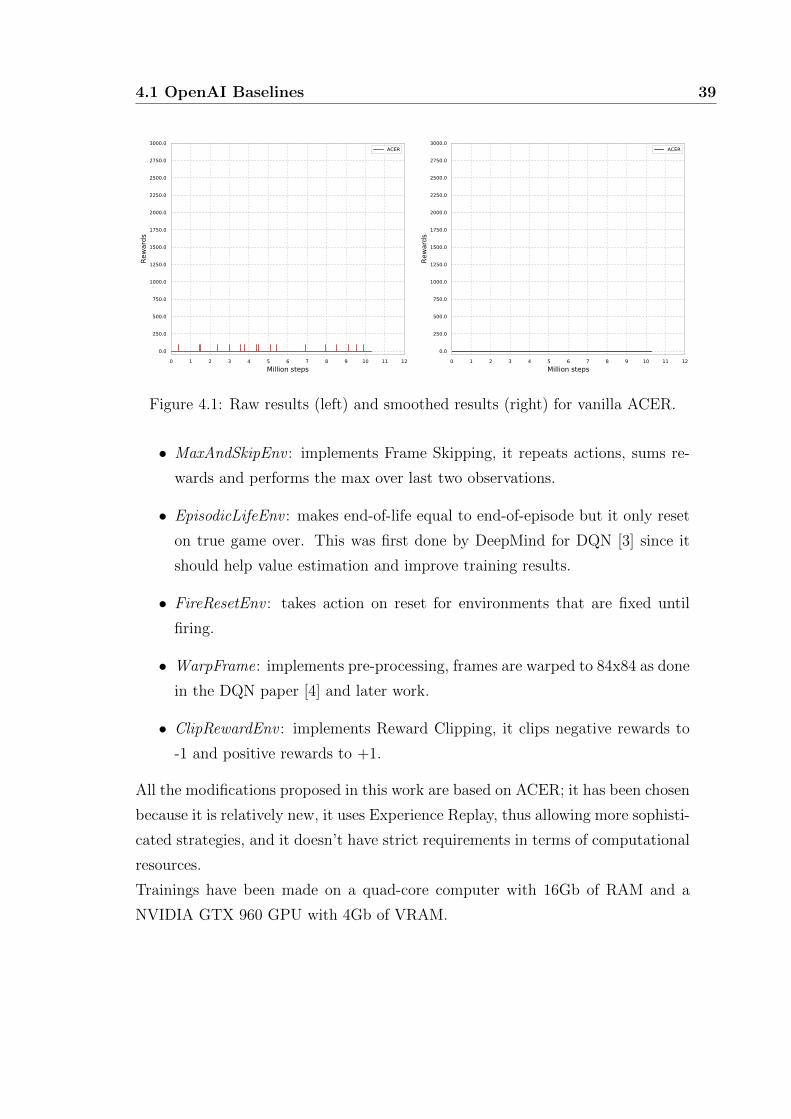
4.1 OpenAI Baselines 39
Figure 4.1: Raw results (left) and smoothed results (right) for vanilla ACER.
• MaxAndSkipEnv : implements Frame Skipping, it repeats actions, sums re-
wards and performs the max over last two observations.
• EpisodicLifeEnv : makes end-of-life equal to end-of-episode but it only reset
on true game over. This was first done by DeepMind for DQN [3] since it
should help value estimation and improve training results.
• FireResetEnv : takes action on reset for environments that are fixed until
firing.
• WarpFrame: implements pre-processing, frames are warped to 84x84 as done
in the DQN paper [4] and later work.
• ClipRewardEnv : implements Reward Clipping, it clips negative rewards to
-1 and positive rewards to +1.
All the modifications proposed in this work are based on ACER; it has been chosen
because it is relatively new, it uses Experience Replay, thus allowing more sophisti-
cated strategies, and it doesn’t have strict requirements in terms of computational
resources.
Trainings have been made on a quad-core computer with 16Gb of RAM and a
NVIDIA GTX 960 GPU with 4Gb of VRAM.

40 4. 3B-ACER
The operating system installed is a Linux distribution with official NVIDIA drivers
and CUDA as well as Python3 and all modules needed to install Gym and Base-
lines (including Tensorflow library).
In order to test Baselines and all remaining software we trained ACER with V0
and V4 environments on Space Invaders for 10 millions steps and we compared
results with those declared in the official papers [32] and online benchmarks. The
scores obtained were in line with official and unofficial ones, this proved the relia-
bility of the base implementation which has been used for all the subsequent tests.
We then tested vanilla ACER on Montezuma’s Revenge for 10 millions steps ob-
taining the results reported in Figure 4.1. In the figure are reported raw and
smoothed results, the least are obtained applying symmetric EMA smoothing di-
rectly implemented in Baselines. On this game the base implementation doesn’t
learn and reaches a positive reward randomly only a few times. In order to prove
that learning doesn’t start with more training time we tried to run ACER for 100
millions steps obtaining the same results.
Inspired by the work of Dubey et al. [41] we investigated on providing knowledge
for the neural network, in particular it is interesting to know if incorporating ob-
ject detection capabilities would improve the learning process. The cited work
investigates on the impact of human prior knowledge on the learning process. In
particular, when looking at an observation, artificial agents see only a bunch of
pixels and they are only able to search for recurrent patterns. Human agents can
natively recognize different objects and they can use this valuable informations
to make more high level planning. It is interesting to note that, when an human
agent cannot distinguish objects, its performance get worse while the behaviour of
an artificial agent remains the same even altering deeply the visual representation
of the states.
Object detection can be very difficult and unreliable in real world problems and
the only simple strategy that can be used is Template Matching; this technique is
implemented in different Computer Vision libraries [42]. It is however very lim-
ited, in fact changing size or other visual features of the objects can easily fool the
recognizer. Due to the limitations of the recognizing algorithm and the magnitude

4.2 Episodic Lifes 41
of the required study, the use of additional knowledge is left to future research. For
all the tests we present from now on we used the default ACER parameters and we
started every training using 16 parallel actors. We changed only the behaviour of
the algorithm as well as the size of the allocated memory and the code that rules
when start to replay. We wanted to maintain all defaults parameters because tun-
ing ACER on a specific problem like Montezuma’s Revenge was out of the scope
of this work. In table A.1 is reported the complete list of fixed hyperparameters
for all the experiments.
ACER makes one on-policy call and a number of off-policy calls dependent on the
replay-ratio number, this is fixed to 4 as in the original paper [8] and it proved to
be the best for Atari games. During an on-policy call ACER collects a batch of
subsequent transitions for each thread, the default size is 20 which is also used in
this work. Each thread stores its batch in its replay buffer and updates the net-
work using it. When an off-policy call is made each thread retrieves a batch from
its replay buffer and uses it to learn. Experiences are fetched independently for
each thread but ACER always stores and retrieves the same amount of transitions
at every call (on-policy and off-policy).
One important thing of this ACER implementation is the replay buffer manage-
ment, it is implemented as a circular buffer where batches are stored sequentially.
Each thread has its own dedicated area in the replay buffer; it is similar to a FIFO
queue so, if an insertion is made and the buffer is full, the oldest batches are over-
written. If a thread inserts two different batches in its buffer these will be stored
sequentially.
4.2 Episodic Lifes
In the original DQN paper [3], in games where there is a life counter, the
number of lives left in the game sent by Atari emulator is then used to mark the
end of an episode during training. This is made to improve the final performance
because it seems to accelerate training speed.
Since results with the original ACER implementation were very poor we wanted

42 4. 3B-ACER
Figure 4.2: Raw results (left) and smoothed results (right) for ACER with Episodic
Game.
to investigate if marking the end of an episode using the end-of-game signal can
improve training. We modified ACER implementation signalling the end of an
episode when the current game ends and the six available lives are lost; we denote
this modification as Episodic Game.
In Figure 4.2 are shown the results of the training with Episodic Game on V4
environment. The outcomes are similar to those we have seen for vanilla ACER
and the agent continues to play randomly after 10 millions steps. In this case,
where rewards are sparse and the agent doesn’t learn anything, changing when the
episode ends doesn’t improve training results.
4.3 Negative Rewards
Another interesting aspect of this game, as well as other games where multi-
ple lives are available, is the use of negative rewards. Since the original work of
DQN [4] almost no study uses negative rewards. Instead, as we have seen before,
on a life loss they end the current episode.
In order to check the impact of negative rewards on training we have modified
ACER and assigned a negative reward of -1 every time that a life is lost, in this

4.4 Best Replay 43
Figure 4.3: Raw results (left) and smoothed results (right) for ACER with negative
rewards.
case we also ended the episode as in the original version of the algorithm. Results
are reported in Figure 4.3, the final agent doesn’t behaves randomly but it tries to
survive. The length of an episode grows during training and the resulting agent,
after selecting a large number of unnecessary actions, reaches the first reward (the
key) and occasionally the second one (one of the doors).
Overall it performs better than the original ACER agent, probably because the
path in the first room of the game is fixed and learning to not die leads indi-
rectly to rewards. Negative rewards, despite performing better, leads to unwanted
behaviours such as long sequences of useless and repeated actions so they don’t
represent an interesting improvement. A further test was made combining nega-
tive rewards and Episodic Game but it led to the same results that we have just
discussed.
4.4 Best Replay
In a game like Montezuma’s Revenge there are only a few episodes that con-
tains one or more positive rewards. When an episode like this is inserted in the
replay buffer, it is quickly overwritten by other less meaningful samples.

44 4. 3B-ACER
Br
rcr = 1
Be
rce = 2
Be
rce = 0
rcr = 2
Br
Figure 4.4: Buffers state before (left) and after (right) an episode replacement in
ACER with Best Replay. Coloured boxes are sample trajectories and gray boxes
represent the unused space in a buffer.
One way to preserve the rare good experiences is to use a dedicated replay buffer.
The first modification that implements this idea is what we call Best Replay. We
have modified ACER so that it uses two buffer instead of one. In the first buffer,
which is a sort of short memory, samples are collected for all threads until the
current episode ends. We denote the short memory buffer as Be. The other buffer,
which we call Br, is the only one used for replay and contains the best episode
experienced. For each thread i we denote Bei as its dedicated short memory buffer
and Bri as its dedicated replay buffer. We also denote len(B) as the number of
elements contained in a generic buffer B. Each buffer maintains a reward counter
for the stored episode, we denote these as rcei and rcri respectively. Once the
episode ends the amount of rewards rcei is compared to rcri . If rcei > rcri then
the replay buffer is overwritten with the content of short memory buffer while if
rcei < rcri the content of Bei is simply discarded.
What if the rewards counters are equal? In this case if rcei ≥ 0 and len(Bei) <
len(Bri) the replay buffer is overwritten because generally a trajectory that leads
to the same amount of positive rewards in a smaller number of steps is better.
The replay buffer is overwritten even if rcei < 0 and len(Bei) > len(Bri) because a
longer trajectory means that the agent dies less frequently. Once the comparison
ends the short memory buffer is cleared. Figure 4.4 illustrates the content replace-
ment of Br.
The original ACER buffer contains 50000 elements for each thread, we wanted to

4.4 Best Replay 45
maintain a similar amount of allocated memory so we made the two buffers of size
30000 elements for each thread.
Replay starts when there is at least one element in the replay buffer for each paral-
lel actor. Every time a replay is performed a random batch from the replay buffer
of each thread is selected. In vanilla ACER replay starts when there are at least a
minimum number of elements in any thread buffer. In fact there is only one buffer
and batches are inserted at the same time for all threads, thus len(Bri) is equal for
any thread i after performing a training step. In Best Replay every thread buffer
can grow independently from the others so we had to heavily change the original
implementation. We changed the replay start policy because with the original one
replay would never start. In fact, if only the best episode is maintained, only a
small number of batches are stored in the buffer and the length of the memorized
sequence could change in time.
In ACER, as we have already seen before, for each update a fixed number of sam-
ples are used, typically a batch of 20 samples for each thread, for a total batch
size of 320 in case of 16 parallel actors. In order to speed up the learning process
we made another modification to ACER: for each batch we modified rewards and
end-of-episode signal. The idea is to fix the value of the last transition contained
in the most important batches (the ones that leads to a positive reward in the cur-
rent episode), it is then propagated using the Retrace algorithm without directly
modifying rewards of the intermediate experiences. In order to better understand
the principle behind this we report a piece of the original pseudo-code of ACER:
Qret ←
{0 for terminal xk∑
aQθ′v(xk, a)f(a|φθv(xk)) otherwise
}...
Qret ← ri + γQret
This piece of pseudo-code calculates the initial Qret value for the first transition of
each thread in the batch, this is used to recursively obtain approximatedQret values
for all the others state-action pairs in the batch. Since we store the best episode
experienced we have enough informations about the value of all the transitions that

46 4. 3B-ACER
Reward End-of-episode
0 False
0 True
0 False
1 False
0 False
0 False
0 False
1 False
0 False
0 False
0 False
0 False
Reward End-of-episode
0 False
0 True
0 False
1 False
0 False
0 False
0.9702 True
1 False
0 False
0.9801 True
0 False
0 False
Table 4.1: An example of Value Fixing applied on four consecutive batches (each
batch here is composed of 3 steps). In this case the values 0.9801 and 0.9702 are
obtained applying the discount factor γ = 0.99 three and two times respectively.
are part of it. Before replacing the content of Bri with the one contained in Bei ,
we overwrite the last element in each batch with the discounted reward calculated
recursively from the end of the episode and we mark it as terminal. Every time that
a positive reward is encountered in the sequence it re-initialize the reward counter
used for the calculation. If the last element of a batch has a positive reward it
remains unchanged. Batches that don’t lead to positive rewards but only to a
terminal state are not modified. With this modification we are simulating an end-
of-episode after almost every batch and we are implicitly imposing a value for every
transition that is part of a positive sequence. We expected that this would improve
the learning speed. Table 4.1 illustrates the modification of a generic sequence
stored in the short memory buffer before its insertion in the replay buffer. We will
call this technique Value Fixing. In order to start replay earlier the first positive
episode is used to initialize the replay buffer of all threads.

4.4 Best Replay 47
Figure 4.5: Raw results (left) and smoothed results (right) for ACER with Best
Replay and Value Fixing.
We expected that replaying often the best samples would improve training speed
and make the agent learn from the best experience made.
We tested this modification without negative rewards and the results were very
bad. We trained the algorithm on the V4 environment for 10 millions steps. As
we can see from Figure 4.5 the algorithm doesn’t learn anything and it reaches
only a few rewards.
We tried also the same procedure without Value Fixing, results are shown in
Figure 4.6 and are very similar the previous ones. Both the agents first obtain
some rewards but later they behave worse than the random agent and they cannot
reach any other positive reward. After the training we tested the resulting agent
and what we observed is that the agent’s behaviour is biased. For example it
remains stuck for a while near the left door probably because it is visually close
to the key. Continuously replaying from the same set of experiences makes the
network overfit, as it tries to learn very well a particular trajectory but it is not
able to generalize. It mistakes the real value of a state and this introduces bias in
the agent behaviour that performs worse than the random one.
We made also one last test to understand if adding experiences in Br instead of
replacing can be beneficial. The last modification is based on the first version of

48 4. 3B-ACER
Figure 4.6: Raw results (left) and smoothed results (right) for ACER with Best
Replay.
the code with Value Fixing, in this case episodes are inserted in the replay buffer
and don’t replace its previous content.
The results obtained are even worse than those we have discussed before. In all
the tests made there was some sort of instability, sometimes gradients and various
other related parameters increased even reaching very high values. This trend is
particularly evident in the last test we made, in this case the instability is so high
that Tensorflow crashed because a tensor reached infinite value. This phenomenon
is known as exploding gradient. It is known that replaying highly correlated samples
is inefficient and leads to high variance of the updates. It could be the cause of
this behaviour although a gradient explosion like the one we have noticed was not
expected and completely unjustified.
Assuming that the problem depends on replaying continuously similar samples,
the catastrophic performances of the last experiment could be justified. This
modification replays continuously the same experiences like the others but, even
when other good episodes are collected, the oldest samples remain in Br; it follows
that there are even more chances that similar batches are replayed at the same
time.

4.5 Triple Buffer 49
Be
Bp
Bn
Figure 4.7: An episode is divided between Bp and Bn in 3B-ACER. Before being
splitted and inserted the episode could be modified with Value Fixing. Coloured
boxes are sample trajectories, light grey boxes represent the unused space in a
buffer and dark gray boxes model the previous content of a buffer.
4.5 Triple Buffer
In order to overcome the issue we discussed in the last section we introduced a
new version that makes use of both positive and less meaningful experiences, we
called this Triple Buffer. We wanted to limit the total amount of allocated mem-
ory, thus we limited each buffer size to 25000 elements for each thread, memory
consumption raised but it never exceeded the total amount of RAM (16Gb).
In this version one buffer is used as short memory buffer, which we will call Be,
and the other two buffers are dedicated to positive and non-positive experiences.
We will call the positive buffer as Bp and the non-positive buffer Bn. The current
episode is stored in Be, once it ends it is analyzed and divided in the other buffers.
All the sample batches that are collected before a positive payoff, thus being part
of a path to a positive reward, or including it, are inserted in Bp. The remaining
batches that don’t lead to anything but a terminal state are inserted in Bn.
In this version there is not content replacement in Bp and Bn but batches are
sequentially added, once a buffer is full and a batch insertion is made the oldest
experiences are lost. In Figure 4.7 is illustrated the division of an episode between
the buffers.

50 4. 3B-ACER
Figure 4.8: Raw results on V4 (left) and V0 (right) environments for 3B-ACER
with Value Fixing.
During replay, for each thread, a batch of samples is independently selected from
its own Bp or Bn.
Each thread i select buffer Bpi with a probability Pi that is proportional to the
number of elements contained in Bpi and is defined as:
Pi =len(Bpi )
len(Bpi )+len(Bni )
Buffer Bni is instead selected with probability 1 − Pi. For example, if thread i
has both Bpi and Bni of equal sizes, the algorithm selects for this thread a batch
from the positive buffer with probability of 50%. Once Bpi or Bni is selected for
sampling, the algorithm chooses a random element within the buffer. Using this
sampling strategy each batch contained in replay buffers has the same chances to
be selected. Mixing positive and non-positive experiences without making pref-
erences reduces correlation between samples during updates. The replay buffers
can be seen as a unique replay memory; this algorithm, which we will call Triple
Buffer ACER or 3B-ACER, is the most similar to the original one.
In vanilla ACER replay starts when replay buffer contains at least rs = 10000 tran-
sitions for each thread. This is made because replaying experiences when there
isn’t even one batch that could be used to learn useful informations is useless.

4.5 Triple Buffer 51
In 3B-ACER replay starts when at least one thread has found a positive reward
(the corresponding Bpi is not empty) and len(Bpi)+ len(Bni) > rs with rs = 5000.
We chose threshold rs to make replay start earlier: this could speed up learning in
the first phase where there are only a few transitions in Bp. In fact initially they
could be replayed more frequently with a lower value of rs.
In the first experiment we combined 3B-ACER with Value Fixing, blocks are mod-
ified before they are inserted in Bp. Unlike the original Value Fixing, during the
backward reward calculation, when a positive reward is encountered its value is
added to the current one. With this modification a sample that is part of a path
to multiple positive rewards has a higher value and it is a better approximation of
the real one.
We tested the algorithm on both V4 and V0 environment for 50 million steps.
Figure 4.8 shows the results for the test made on V4 environment, they are very
good and the agent consistently reaches 2500 points and occasionally even more.
We inspected the behaviour of the resulting agent and it plays very well, in the
first room it reaches the key and the door on the right without touching the skull.
It then moves in the right room avoiding the enemies, it goes downstairs reaching
the third room and it obtains a weapon. After achieving three rewards it goes
upstairs and kills one enemy with the weapon obtaining its fourth reward.
After these good results confirmed by subsequent tests we tried 3B-ACER with
Value Fixing on V0 environment. In this case the results, which are reported in
Figure 4.8 as before, were different and unexpected. Despite learning very quickly
it reaches 400 points and it never further improves. We inspected the behaviour
of the resulting agent and we noted that, after obtaining the key and returning at
the starting point without dying, it always chooses the left door. From this point
it cannot go right and the lasers on the left are too difficult to cross. We repeated
this experiment three times obtaining always the same results.
In order to overcome this problem we tested different solutions. At the beginning
of this work we modified ACER to make the end-of-game signal equal to end-
of-episode signal. We now have a modification that effectively learns and makes
average scores greater than 0 points. We combined 3B-ACER with Value Fixing,

52 4. 3B-ACER
Best Replay and Episodic Game. In this version Bp contains the best experiences
collected over an entire game while Bn contains all the other batches.
The current episode, which is a complete game, is stored in Be and, when the
episode ends, the total rewards obtained is compared with the maximum achieved.
If the total rewards exceed the maximum obtained, the current episode replaces
the content of Bp and its reward counter is updated. If rewards are equal to the
maximum, the content of Be is inserted in Bp without replacing its content. In
both cases before replacing or inserting Value Fixing (the last version) is applied
and the episode is divided between Bp and Bn as we have seen before. The tra-
jectory that leads to at least a positive reward goes in Bp and any trajectory that
leads to a terminal state without encountering a positive reward goes in Bn. If
current rewards are lower than the maximum the entire episode is inserted in Bn.
This modification tries to replay frequently batches that leads to positive rewards
taking in consideration the real value of a reward. If we want to replay frequently
only the best sequences possible we want to consider rewards that are reached in
multiple lives. For example, if the agent reaches two rewards in a life and a third
one in another life and previously it has reached less than three rewards in a game,
we want to learn this new trajectory entirely, discarding all previous and less valu-
able experiences. By combining episodic game and Value Fixing and maintaining
only the best sequences of batches we were hoping to overcome the problems we
have discussed with the previous case. Unfortunately results were even worse and
the agent reached consistently 400 points with both V4 and V0 environment. It
shows the same strange behaviour of the previous case and it always chooses the
left door.
The reason behind this behaviour could be the Value Fixing technique we were
using. V4 environment is almost completely deterministic, if a sequence of actions
leads to a reward once then most likely it will do so in the future as well. Thus
the value of transitions we were imposing can be a good approximation of the real
value.
The V0 environment is much less deterministic and an action can lead to a differ-
ent state from time to time. Value Fixing can lead to an overestimation in these

4.5 Triple Buffer 53
Figure 4.9: Raw results (left) and smoothed results (right) for 3B-ACER in V0
environment.
conditions because the behaviour of the underlying environment is not known. A
particular state-action trajectory can lead to a reward once but this does not guar-
antee that it will happen again, even if repeated multiple times. This can justify
the biased behaviour of the agent with the V0 environment. 3B-ACER with Value
Fixing can be a good choice in case of an almost perfectly known environment
reaching the same score obtained by other algorithms that are more competitive
than vanilla ACER.
Since Value Fixing introduces biases in the agent’s behaviour we tested the orig-
inal 3B-ACER without using this technique in both V4 and V0 environments for
50 millions steps. Results are reported in Figure 4.9, in this case the agent learns
more slowly than it did previously and the algorithm reaches only 500 points. It is
however more reliable than the previous modification because it reaches the same
results in both the environments. We made more tests to see if it can reliably
reproduce the results and we observed that it isn’t perfect. Learning starts when
the positive buffer contains a sufficient number of elements and the probability of
selecting a sample from Bp becomes sufficiently high. In the initial learning phase
the agent behaves randomly thus positive trajectory are not found always at the
same rate. The time needed to start learning is very variable, in one test it hasn’t

54 4. 3B-ACER
Figure 4.10: Raw results (left) and smoothed results (right) for 3B-ACER with
Half Replay in V4 environment.
started learning even after 50 millions steps. After the good results we obtained
with 3B-ACER the biggest problem was to speed up learning in the first phase.
The positive buffer must contain a sufficient number of elements to start the learn-
ing phase. In order to overcome this problem we tried two different sample policies,
we call these Sequence sampling and Half sampling. In Sequence sampling once
Bp is selected as the sampling buffer (using the number of elements contained) the
algorithm does not choose a random element but it uses an internal reference to
retrieve batches in sequence. We wanted to implement this sampling strategy be-
cause sampling positive experiences sequentially could propagate faster the value
of a state and thus speed up learning. We tested this modification for 50 millions
steps in both V4 and V0 environment but the results are almost identical to the
original 3B-ACER. The algorithm reaches good scores (500 points) but the time
needed to start learning is variable.
The last modification, Half sampling, is an interesting one. In this case both
buffers are chosen with a probability Pi = 50%. During the initial phase of learn-
ing a few elements are contained in Bp so, using this strategy, these are replayed
much more frequently than in the original 3B-ACER. As the number of elements
increases each positive sample is replayed less and less frequently.
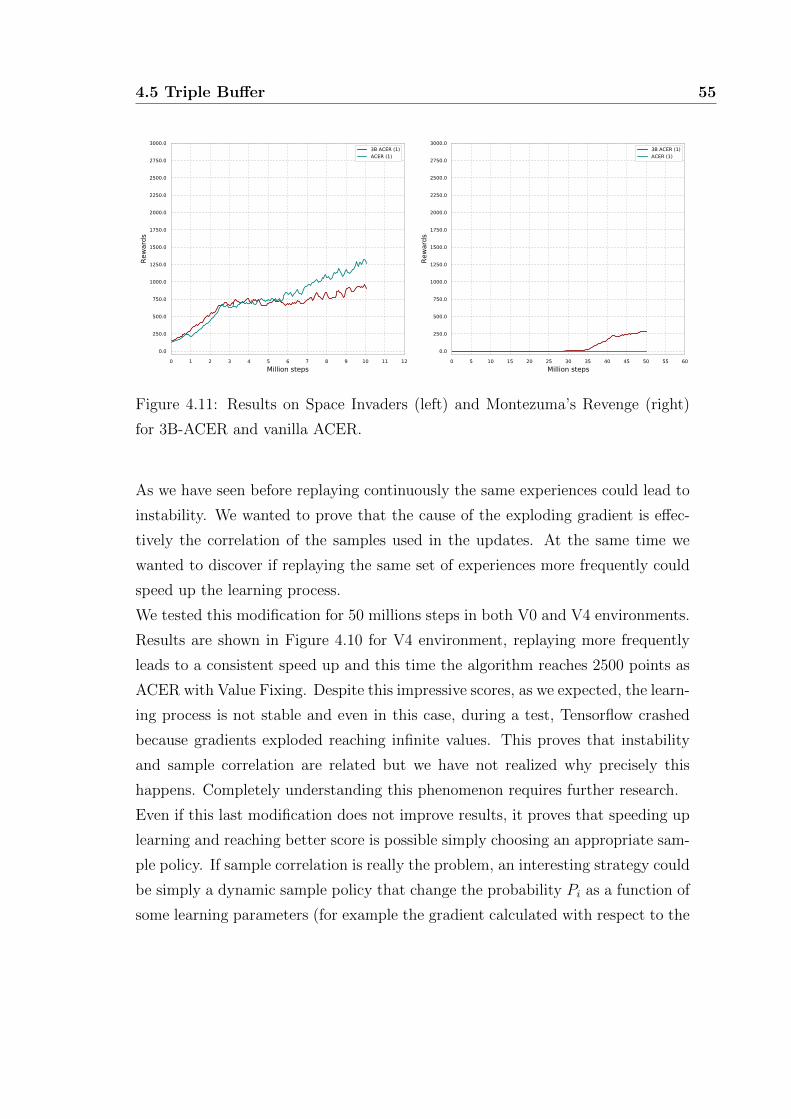
4.5 Triple Buffer 55
Figure 4.11: Results on Space Invaders (left) and Montezuma’s Revenge (right)
for 3B-ACER and vanilla ACER.
As we have seen before replaying continuously the same experiences could lead to
instability. We wanted to prove that the cause of the exploding gradient is effec-
tively the correlation of the samples used in the updates. At the same time we
wanted to discover if replaying the same set of experiences more frequently could
speed up the learning process.
We tested this modification for 50 millions steps in both V0 and V4 environments.
Results are shown in Figure 4.10 for V4 environment, replaying more frequently
leads to a consistent speed up and this time the algorithm reaches 2500 points as
ACER with Value Fixing. Despite this impressive scores, as we expected, the learn-
ing process is not stable and even in this case, during a test, Tensorflow crashed
because gradients exploded reaching infinite values. This proves that instability
and sample correlation are related but we have not realized why precisely this
happens. Completely understanding this phenomenon requires further research.
Even if this last modification does not improve results, it proves that speeding up
learning and reaching better score is possible simply choosing an appropriate sam-
ple policy. If sample correlation is really the problem, an interesting strategy could
be simply a dynamic sample policy that change the probability Pi as a function of
some learning parameters (for example the gradient calculated with respect to the

56 4. 3B-ACER
value function). If these are in a determined range we simply choose Pi = 50%, as
parameters values start to rise we lower the probability until reaching a minimum
value. This minimum value could be the probability normally used in the original
3B-ACER (dependent on the number of elements contained).
In conclusion in deterministic environments 3B-ACER with Value Fixing is the
variant that has reached the best results but it is unreliable in more complex and
realistic problems. In more unpredictable environments plain 3B-ACER is the best
algorithm that, with a proper sample policy, could reach scores similar to those
obtained by much more modern works.
As a final test we wanted to discover plain 3B-ACER performances in general
problems so we tested it in a dense reward problem. We tested 3B-ACER on
Space Invaders because it is commonly used as benchmark. We trained the algo-
rithm on V0 environment for 10 millions steps because they are sufficient to make
a comparison (due to limited time and resources). Results are reported in Figure
4.11 where we compared 3B-ACER and vanilla ACER on Montezuma’s Revenge
and Space Invaders. As we can see from the figure 3B-ACER performs well also
on dense reward problem like Space Invaders obtaining similar scores. Results
obtained are slightly worse for 3B-ACER probably because in vanilla ACER a
large portion of the replay buffer contains positive experiences. In 3B-ACER the
size of the replay buffer used for positive experiences is halved thus every positive
transition has less chances to be replayed. While it doesn’t outperform the state
of the art, 3B-ACER is an interesting improvement of the original ACER and it
could perform even better with further research.

Conclusions
In this work we presented a complete introduction to Reinforcement Learning
and we discussed different kind of problems. We described the main approaches
to RL and the most influential algorithms.
We introduced OpenAI Gym [10], an important tool that is commonly used to
benchmark RL algorithms. We presented OpenAI Baselines [35] that represents
an interesting suite of algorithms that could be used to learn various tasks or as a
base for more advanced solutions.
Starting from the OpenAI ACER [8] implementation we proposed and tested var-
ious ideas used to improve the original algorithm. We found that two major ideas
can improve the base method: ACER with Value Fixing and 3B-ACER.
ACER with Value Fixing exploits the determinism of the environment and reaches
score similar to more modern algorithms but it is inadequate in non deterministic
environments. In these conditions the agent’s behaviour is biased and further re-
search is needed to completely understand the causes of this strange result.
3B-ACER learns much more slowly but it is usable in both deterministic and non-
deterministic environments, moreover the time needed to start learning is variable.
We discovered that 3B-ACER combined with a proper sample policy could learn
much faster and reach scores similar to those obtained by ACER with Value Fix-
ing.
Designing a good sample policy requires completely understanding the exploding
gradient phenomenon and how sample correlation in updates could make Tensor-
flow crash, further research is needed in this direction.
57

58 CONCLUSIONS
Here we report a list of possible improvements of this work:
• Try different problems, we made tests only on two games but OpenAI Gym
offers a large number of interesting tasks. In order to show the real perfor-
mance of 3B-ACER we need to test it on a large variety of problems. We
expect that it would perform similar to, or even better than, the original
ACER on a large portion of the tasks.
• Study a new sample policy that speed up the learning process of 3B-ACER,
namely by filling the positive buffer more quickly until it contains a sufficient
number of elements.
• Combine Experience Replay and Triple Buffer with a more modern and intu-
itive algorithm like PPO [32], with a more modern base algorithm combined
with the ideas we have seen it could be much more sample efficient and it
could perform very well on a large variety of tasks.
• Insert prior knowledge: human agents have innate skills like object detection
that represent a huge advantage respect to modern RL algorithms. What an
artificial agent “sees” is just a bunch of pixels, it searches for recurrent pat-
terns and no more. We instead are able to recognize objects and understand
that they are points of interest, this lead to a more sophisticated planning.
Inserting prior knowledge, like adding positions and shapes of objects as
input informations, could make the agent learn much more efficiently.

Appendix A. Hyperparameters
Hyperparameter Value
Number of steps per batch 20
Frame stack 4
γ 0.99
α 0.99
δ 1
Learning rate 0.0007
Gradient norm clipping coeff. 10
Entropy coefficient 0.01
Value function loss coeff. 0.5
IS weight clipping factor 10
RMSProp α 0.99
RMSProp ε 0.00001
Trust region Yes
Replay ratio 4
Frame skipping 4
Number of parallel actors 16
Network architecture CNN
Table A.1: ACER default hyperparameters used in all experiments made.
59

Appendix B. Scores
Agent Score
Human average [31] 4753
Human Expert [31] 34900
Human World Record [31] 1219200
DQN [3] 0
A3C [9] 67
ACER [8] 0.3
DDQN-CTS [23] 3705.5
A3C-CTS [23] 1127
DQN-PixelCNN [24] 2514.3
The Reactor [25] 2643.5
Feature-EB [26] 2745.4
Deep-CS [29] 2504.6
UBE [27] 3000
Ape-X [28] 2500
PPO [30] 2497
RND [30] 8152
Go-Explore [31] 43763
Table B.1: Best results on Montezuma’s Revenge.
60
Bibliography
[1] Richard S Sutton and Andrew G Barto. Reinforcement learning: An intro-
duction. MIT press, 2018.
[2] Yuxi Li. Deep reinforcement learning: An overview. arXiv preprint
arXiv:1701.07274, 2017.
[3] Volodymyr Mnih, Koray Kavukcuoglu, David Silver, Andrei A Rusu, Joel Ve-
ness, Marc G Bellemare, Alex Graves, Martin Riedmiller, Andreas K Fidje-
land, Georg Ostrovski, et al. Human-level control through deep reinforcement
learning. Nature, 518(7540):529, 2015.
[4] Volodymyr Mnih, Koray Kavukcuoglu, David Silver, Alex Graves, Ioannis
Antonoglou, Daan Wierstra, and Martin Riedmiller. Playing atari with deep
reinforcement learning. arXiv preprint arXiv:1312.5602, 2013.
[5] David Silver, Aja Huang, Chris J Maddison, Arthur Guez, Laurent Sifre,
George Van Den Driessche, Julian Schrittwieser, Ioannis Antonoglou, Veda
Panneershelvam, Marc Lanctot, et al. Mastering the game of go with deep
neural networks and tree search. nature, 529(7587):484, 2016.
[6] David Silver, Julian Schrittwieser, Karen Simonyan, Ioannis Antonoglou, Aja
Huang, Arthur Guez, Thomas Hubert, Lucas Baker, Matthew Lai, Adrian
Bolton, et al. Mastering the game of go without human knowledge. Nature,
550(7676):354, 2017.
[7] Long-Ji Lin. Self-improving reactive agents based on reinforcement learning,
planning and teaching. Machine learning, 8(3-4):293–321, 1992.
61

62 BIBLIOGRAPHY
[8] Ziyu Wang, Victor Bapst, Nicolas Heess, Volodymyr Mnih, Remi Munos,
Koray Kavukcuoglu, and Nando de Freitas. Sample efficient actor-critic with
experience replay. arXiv preprint arXiv:1611.01224, 2016.
[9] Volodymyr Mnih, Adria Puigdomenech Badia, Mehdi Mirza, Alex Graves,
Timothy Lillicrap, Tim Harley, David Silver, and Koray Kavukcuoglu. Asyn-
chronous methods for deep reinforcement learning. In International conference
on machine learning, pages 1928–1937, 2016.
[10] Greg Brockman, Vicki Cheung, Ludwig Pettersson, Jonas Schneider, John
Schulman, Jie Tang, and Wojciech Zaremba. Openai gym. arXiv preprint
arXiv:1606.01540, 2016.
[11] Marlos C Machado, Marc G Bellemare, Erik Talvitie, Joel Veness, Matthew
Hausknecht, and Michael Bowling. Revisiting the arcade learning environ-
ment: Evaluation protocols and open problems for general agents. Journal of
Artificial Intelligence Research, 61:523–562, 2018.
[12] Gerald Tesauro. Td-gammon, a self-teaching backgammon program, achieves
master-level play. Neural computation, 6(2):215–219, 1994.
[13] Matej Moravcık, Martin Schmid, Neil Burch, Viliam Lisy, Dustin Morrill,
Nolan Bard, Trevor Davis, Kevin Waugh, Michael Johanson, and Michael
Bowling. Deepstack: Expert-level artificial intelligence in heads-up no-limit
poker. Science, 356(6337):508–513, 2017.
[14] Yuxin Wu and Yuandong Tian. Training agent for first-person shooter game
with actor-critic curriculum learning. ICLR 2017, 2016.
[15] Peng Peng, Quan Yuan, Ying Wen, Yaodong Yang, Zhenkun Tang, Haitao
Long, and Jun Wang. Multiagent bidirectionally-coordinated nets for learning
to play starcraft combat games. arXiv preprint arXiv:1703.10069, 2, 2017.
[16] Hado Van Hasselt, Arthur Guez, and David Silver. Deep reinforcement learn-
ing with double q-learning. In Thirtieth AAAI Conference on Artificial Intel-
ligence, 2016.

BIBLIOGRAPHY 63
[17] Ziyu Wang, Tom Schaul, Matteo Hessel, Hado Van Hasselt, Marc Lanctot,
and Nando De Freitas. Dueling network architectures for deep reinforcement
learning. arXiv preprint arXiv:1511.06581, 2015.
[18] Tom Schaul, John Quan, Ioannis Antonoglou, and David Silver. Prioritized
experience replay. arXiv preprint arXiv:1511.05952, 2015.
[19] Richard S Sutton, David A McAllester, Satinder P Singh, and Yishay Man-
sour. Policy gradient methods for reinforcement learning with function ap-
proximation. In Advances in neural information processing systems, pages
1057–1063, 2000.
[20] John Schulman, Sergey Levine, Pieter Abbeel, Michael I Jordan, and Philipp
Moritz. Trust region policy optimization. In Icml, volume 37, pages 1889–
1897, 2015.
[21] Remi Munos, Tom Stepleton, Anna Harutyunyan, and Marc Bellemare. Safe
and efficient off-policy reinforcement learning. In Advances in Neural Infor-
mation Processing Systems, pages 1054–1062, 2016.
[22] A. Asperti, D. Cortesi, C. de Pieri, G. Pedrini, and F. Sovrano. Crawling in
rogue’s dungeons with deep reinforcement techniques. IEEE Transactions on
Games, pages 1–1, 2019.
[23] Marc Bellemare, Sriram Srinivasan, Georg Ostrovski, Tom Schaul, David
Saxton, and Remi Munos. Unifying count-based exploration and intrinsic
motivation. In Advances in Neural Information Processing Systems, pages
1471–1479, 2016.
[24] Georg Ostrovski, Marc G Bellemare, Aaron van den Oord, and Remi Munos.
Count-based exploration with neural density models. In Proceedings of the
34th International Conference on Machine Learning-Volume 70, pages 2721–
2730. JMLR. org, 2017.
[25] Audrunas Gruslys, Will Dabney, Mohammad Gheshlaghi Azar, Bilal Piot,
Marc Bellemare, and Remi Munos. The reactor: A fast and sample-efficient

64 BIBLIOGRAPHY
actor-critic agent for reinforcement learning. In International Conference on
Learning Representations, 2018.
[26] Jarryd Martin, Suraj Narayanan Sasikumar, Tom Everitt, and Marcus Hutter.
Count-based exploration in feature space for reinforcement learning. arXiv
preprint arXiv:1706.08090, 2017.
[27] Brendan O’Donoghue, Ian Osband, Remi Munos, and Volodymyr Mnih.
The uncertainty bellman equation and exploration. arXiv preprint
arXiv:1709.05380, 2017.
[28] Dan Horgan, John Quan, David Budden, Gabriel Barth-Maron, Matteo Hes-
sel, Hado Van Hasselt, and David Silver. Distributed prioritized experience
replay. arXiv preprint arXiv:1803.00933, 2018.
[29] Yuri Burda, Harri Edwards, Deepak Pathak, Amos Storkey, Trevor Darrell,
and Alexei A Efros. Large-scale study of curiosity-driven learning. arXiv
preprint arXiv:1808.04355, 2018.
[30] Yuri Burda, Harrison Edwards, Amos Storkey, and Oleg Klimov. Exploration
by random network distillation. arXiv preprint arXiv:1810.12894, 2018.
[31] Adrien Ecoffet, Joost Huizinga, Joel Lehman, Kenneth O Stanley, and Jeff
Clune. Go-explore: a new approach for hard-exploration problems. arXiv
preprint arXiv:1901.10995, 2019.
[32] John Schulman, Filip Wolski, Prafulla Dhariwal, Alec Radford, and
Oleg Klimov. Proximal policy optimization algorithms. arXiv preprint
arXiv:1707.06347, 2017.
[33] Arun Nair, Praveen Srinivasan, Sam Blackwell, Cagdas Alcicek, Rory Fearon,
Alessandro De Maria, Vedavyas Panneershelvam, Mustafa Suleyman, Charles
Beattie, Stig Petersen, et al. Massively parallel methods for deep reinforce-
ment learning. arXiv preprint arXiv:1507.04296, 2015.

BIBLIOGRAPHY 65
[34] Google’s Machine Intelligence Research. Tensorflow: an Open Source Machine
Learning Framework for Everyone, 2019. https://github.com/tensorflow/
tensorflow, Last accessed on 2019-02-28.
[35] Prafulla Dhariwal, Christopher Hesse, Oleg Klimov, Alex Nichol, Matthias
Plappert, Alec Radford, John Schulman, Szymon Sidor, Yuhuai Wu, and
Peter Zhokhov. Openai baselines. GitHub, GitHub repository, 2017.
[36] Yuhuai Wu, Elman Mansimov, Roger B Grosse, Shun Liao, and Jimmy Ba.
Scalable trust-region method for deep reinforcement learning using kronecker-
factored approximation. In Advances in neural information processing sys-
tems, pages 5279–5288, 2017.
[37] Timothy P Lillicrap, Jonathan J Hunt, Alexander Pritzel, Nicolas Heess, Tom
Erez, Yuval Tassa, David Silver, and Daan Wierstra. Continuous control with
deep reinforcement learning. arXiv preprint arXiv:1509.02971, 2015.
[38] Jonathan Ho and Stefano Ermon. Generative adversarial imitation learn-
ing. In Advances in Neural Information Processing Systems, pages 4565–4573,
2016.
[39] Marcin Andrychowicz, Filip Wolski, Alex Ray, Jonas Schneider, Rachel Fong,
Peter Welinder, Bob McGrew, Josh Tobin, OpenAI Pieter Abbeel, and Woj-
ciech Zaremba. Hindsight experience replay. In Advances in Neural Informa-
tion Processing Systems, pages 5048–5058, 2017.
[40] Matplotlib Development Team. Matplotlib Python 2D plotting library, 2019.
https://matplotlib.org/, Last accessed on 2019-02-28.
[41] Rachit Dubey, Pulkit Agrawal, Deepak Pathak, Thomas L Griffiths, and
Alexei A Efros. Investigating human priors for playing video games. arXiv
preprint arXiv:1802.10217, 2018.
[42] OpenCV Development Team. Template Matching with OpenCV
2.4, 2019. https://docs.opencv.org/2.4/doc/tutorials/imgproc/

66 BIBLIOGRAPHY
histograms/template_matching/template_matching.html, Last accessed
on 2019-02-28.

Acknowledgements
I’m very thankful to Andrea Asperti for his patience, support and ideas during
this entire period of work.
I also want to thank to my friends and family for supporting me in this long
journey.