experiment- 1 basic operations on...

Basic Simulation Lab

Department of Electronics & Communication Engineering 1

EXPERIMENT- 1

BASIC OPERATIONS ON MATRICES

AIM: Write a program to perform basic operation on matrices.

SOFTWARE REQUIRED: PC loaded with SCILAB software

THEORY:

Vectors are special forms of matrices and contain only one row or one column. Whereas

scalars are special forms of matrices and contain only one row and one column. A matrix

with one row is called row vector and a matrix with single column is called column vector.

PROCEDURE:

1. Click on SCILAB Icon

2. Click on launch scinotes

3. Type the program on editor window

4. Save the program with filename.sce extension

5. Execute the program and observe the output/wave forms

PROGRAM:

A = input('Enter the Matrix A ::');

B = input('Enter the Matrix B ::');

// Find the size of matrices

disp('The size of Matrix A is .... :: ');

disp(size(A));

disp('The size of Matrix B is .... :: ');

disp(size(B));

// Addition of two matrices

disp('Addition of A and B Matrices is .....:: ');

disp(A + B);

// Subtration of two matrices

disp('Subtraction of A and B Matrices is .....:: ');



disp(A - B);

//Multiplication (ELEMENT BY ELEMENT) of two matrices

disp('Multiplication of A and B Matrices is .....:: ');

disp(A .* B);

// Finding the Rank of the matrix

disp('Rank of Matrix A is ::');

disp(rank(A));

// Find the determinant of the matrix

disp('Determinant of Matrix A is ::');

disp(det(A));

// Find the trace of the matrix

disp('Trace of Matrix A is ::');

disp(trace(A));

//Find the Inverse of the matrix

disp('Inverse of Matrix A is ::');

disp(inv(A));

OUTPUT:

Enter the Matrix A ::[1 2 ; 2 3 ; ]

Enter the Matrix B ::[1 2 ; 2 3 ; ]

The size of Matrix A is.... ::

2. 2.

The size of Matrix B is....::

2. 2.

Addition of A and B Matrices is.....::

2. 4.

4. 6.

Subtraction of A and B Matrices is.....::

0. 0.

0. 0.



Multiplication of A and B Matrices is .....::

1. 4.

4. 9.

Rank of Matrix A is ::

2.

Determinant of Matrix A is ::

- 1.

Trace of Matrix A is ::

4.

Inverse of Matrix A is ::

- 3. 2.

2. - 1.

RESULT:

Hence basic operations on matrices are performed

VIVA –VOCE QUESTIONS:

1. Expand SCILAB? And importance of SCILAB?

2. What is clear all and close all will do?

3. What is disp () and input ()?

4. What is the syntax to find the Eigen values and eigenvectors of the matrix?

5. What is the syntax to find rank of the matrix?



EXPERIMENT-2

GENERATION OF SIGNALS AND SEQUENCES

AIM: Write a program to Generate various signals and sequences (Periodic and aperiodic), such

as Unit Impulse, Unit Step, Square, Saw tooth, Triangular, Sinusoidal, Ramp, Sinc.

SOFTWARE REQUIRED: PC loaded with SCI LAB software

THEORY:

If the amplitude of the signal is defined at every instant of time then it is called continuous time

signal. If the amplitude of the signal is defined at only at some instants of time then it is called

discrete time signal. If the signal repeats itself at regular intervals then it is called periodic signal.

Otherwise they are called aperiodic signals.

EX: ramp, Impulse,unit step, sinc- Aperiodic signals

Square, sawtooth, triangular sinusoidal – periodic signals.

Ramp signal: The ramp function is a unitary real function, easily computable as the mean of the

independent variable and its absolute value.This function is applied in engineering. The name

ramp function is derived from the appearance of its graph.

r(t) = t when t≥0

=0 else

Unit impulse signal: One of the more useful functions in the study of linear systems is the "unit

impulse function."An ideal impulse function is a function that is zero everywhere but at the origin,

where it is infinitely high. However, the area of the impulse is finite

Y(t)= 1 when t=0

=0 other wise



Unit step signal: The unit step function and the impulse function are considered to be

fundamental functions in engineering, and it is strongly recommended that the reader becomes

very familiar with both of these functions.

=0 if t < 0

u(t) = 1 if t > 0

=1/2 If t=0

Sinc signal: There is a particular form that appears so frequently in communications engineering,

that we give it its own name. This function is called the "Sinc function”.

PROCEDURE:






PROGRAM:

//continuous ramp signal

t = 0 : 0.001 : 1;

y = 0.5 * t;

plot( t , y );

xlabel ('--------->Time Index t (sec.)');

ylabel ('--------->Amplitude');

title ('Ramp Signal Sequence');

//discrete ramp signal

n = 0 : 0.1 : 1;

y = 0.5 * n;

plot2d3(n,y);

xlabel ('---------->Time Index n');



ylabel ('---------->Amplitude');

title ('Ramp Signal Sequence');

//continuous sinc signal

t=linspace(-10 , 10);

y=sinc(t);

plot(t,y);

xlabel("Time Index t (sec.)");

ylabel("Amplitude");

title("Sinc Signal Sequence");

//discrete sinc signal

n =linspace(-10 , 10);

y =sinc(n);

plot2d3(n,y);

xlabel("Time Index n");

ylabel("Amplitude");

title("Sinc Signal Sequence");

// continuous Sinusoidal Signal

a=input('Enter amplitude');

t=0:0.001:1;

p=a*sin(2*%pi*10*t);

plot(t,p);

title("Sinusoidal sequence");

xlabel("time");

ylabel("amplitude");

// discrete sinuoidal signal

a=input('Enter magnitude');

n = 0:100;

x =a*sin(((2*0.05)*%pi)*n);

plot2d3(n,x);

title("Sinusoidal sequence");

xlabel("samples");

ylabel("magnitude");

// continuous square wave Signal:


t=0:0.001:1;

d=a*squarewave(2*%pi*10*t);

plot(t,d);

xlabel ("---------->Time Index t (sec.)");

ylabel ("---------->Amplitude");

title ("Square Wave Signal Sequence");



// discrete square wave signal


n=0 : 0.01 :1;

d=a*squarewave(2*%pi*10*n);

plot2d3(n,d);

xlabel ("---------->Time Index n");

ylabel ("---------->Amplitude");

title ("Square Wave Signal Sequence");

// Triangular Wave Signal

Fs = 20; // samples per second

t_total = 100; // seconds

n_samples = Fs * t_total;

t = linspace(0, t_total, n_samples);

f=40; // sound frequency

tri_wave=(2/%pi)*asin(sin(2*%pi*f*t));

plot(t,tri_wave);

xlabel ('---------->Time Index t (sec.)');

ylabel ('----------->Amplitude');

title ('Triangular Wave Signal Sequence');

// traiangular wave sequence






tri_wave=(2/%pi)*asin(sin(2*%pi*f*t));

plot(t,tri_wave);

xlabel ('---------->Time Index t (sec.)');

ylabel ('----------->Amplitude');

title ('Triangular Wave Signal Sequence');

// Sawtooth Wave Signal






// Sawtooth wave

saw_wave=2*(f*t-floor(0.5+f*t));

plot(t,saw_wave);

xlabel ("---------->Time Index t (sec.)");

ylabel ("----------->Amplitude");

title ("Sawtooth Wave Signal Sequence");



// sawtooth wave sequence




n = linspace(0, t_total, n_samples);


// Sawtooth wave

saw_wave=2*(f*n-floor(0.5+f*n));

plot2d3(n,saw_wave);

xlabel ("---------->Time Index ");

ylabel ("----------->Amplitude");

title ("Saw tooth Wave Signal Sequence");

// Unit Impulse Signal and Sequence:

t=-5:1:5;

a=[zeros(1,5) 1 zeros(1,5)];

k=input("enter the amplitude");

b=k*a;

subplot(2,1,1);

plot(t,b);

xlabel("impulse response", "amplitude", "time");

subplot(2,1,2);

plot2d3(t,b);

xlabel("impulse response", "amplitude", "time");

// Unit Step Signal and Sequence:

// Discrete Signal

t=0:4;

y=ones(1,5);

subplot(2,1,1);

plot2d3 (t,y);

xlabel('time');

ylabel('amplitude');

title('Unit Step Discrete Signal');

// Continuous Signal

subplot(2,1,2);

plot(t,y);

xlabel('time');


title('Unit Step Continuous Signal');



OUTPUT:



enter the amplitude 9



RESULT:

Hence various signals & sequences are generated using SCILAB software

VIVA QUESTIONS:

1. Define Signal?

2. Define continuous and discrete Signals?

3. State the relation between step, ramp and Delta Functions?

4. Differentiate saw tooth and triangular signals?

5. Define Periodic and aperiodic Signal?



EXPERIMENT -3

OPERATIONS ON SIGNALS & SEQUENCES

AIM: Write a program to perform the operations on signals and sequences such as addition,

multiplication, scaling, shifting, folding and also compute energy and power.

SOFTWARE REQUIRED: PC loaded with SCI LAB software.

THEORY:

Signal Addition

Addition: any two signals can be added to form a third signal,

z (t) = x (t) + y (t)

Multiplication:

Multiplication of two signals can be obtained by multiplying their values at every instants . z

z(t) = x (t) y (t)

Time reversal/Folding:

Time reversal of a signal x(t) can be obtained by folding the signal about t=0.

Y(t)=y(-t)

Signal Amplification/Scaling : Y(n)=ax(n) if a < 1 attnuation

a >1 amplification



Time shifting: The time shifting of x(n) obtained by delay or advance the signal in time by

using y(n)=x(n+k)

If k is a positive number, y(n) shifted to the right i e the shifting delays the signal

If k is a negative number, y(n ) it gets shifted left. Signal Shifting advances the signal

Energy:

Average power:

PROCEDURE:






PROGRAM:

// Addition

x=input('Enter the sequence 1=');

y=input('Enter the sequence 2=');

m=length(x);

n=length(y);

if m>n

y=[y,zeros(1,m-n)];

else

x=[x,zeros(1,n-m)];



end

z=x+y;

disp(z,'Addition result of two unequal length sequences:=');

// Multiplication

x=input('Enter the sequence 1=');

y=input('Enter the sequence 2=');

m=length(x);

n=length(y);

if m>n

y=[y,zeros(1,m-n)];

else

x=[x,zeros(1,n-m)];

end

z = x.*y;

disp (z, ' Multiplication result of two unequal lengths equences:= ' );

// Folding Operation

x = input ( ' Enter the input sequence e := ' );

m = length (x);

s = input ( ' Enter the starting point of original signal=' );

h = s + m -1;

n = s :1: h;

subplot (2 ,1 ,1)

x_location = " o r i g i n ";

y_location = " o r i g i n ";

data_bounds = [ -5 ,0;5 ,5];

plot2d3 (n,x)

xlabel ( ' n===>' )

ylabel ( ' Ampl itude' )

title ( ' Original Sequence ' )

subplot (2 ,1 ,2)



data_bounds = [ -5 ,0;5 ,5];

plot2d3 (-n,x)

xlabel ( ' n===>' )


title ( ' Folded Sequence ' )

// Scaling Operation

x = input( ' Ent e r input Sequence := ' );

m = length(x);

s= input ( ' Enter starting point of originalsignal:= ' )

h = s+m-1;

n = s :1: h;

C = input( 'Ent e r Compression factor Time Scaling factor' )



n = s/C:1/C:h/C ;

subplot (2 ,2 ,3)



data_bounds = [ -10 ,0;10 ,10];

plot2d3 (n,x)

xlabel ( ' n===>' )


title ( ' Time Scaling - Compressed Sequence ' )

// shifting operation

x = input ( ' Enter the input sequence := ' )

m = length (x);

lx = input ( ' Enter the starting point of original signal := ' )

hx = lx+m -1;

n = lx :1: hx;

subplot (3 ,1 ,1)



data_bounds = [ -10 ,0;10 ,10];

plot2d3 (n,x);

xlabel ( ' n===>' )

ylabel ( ' Ampl itdue' )

title ( ' Original Sequence' )

d = input ( ' Enter the delay := ' )

n = lx+d:1: hx+d;

subplot (3 ,1 ,2)



data_bounds = [ -10 ,0;10 ,10];

plot2d3 (n,x)

xlabel ( ' n===>' )

ylabel ( ' Amplitude' )

title ( ' Delayed Sequence ' )

// Energy and Average power

p = input('Enter the sequence ...:: ');

M = length(p);

disp(M)

sum = 0;

for i = 1:M,

sum=sum +(i*i);

end;

disp('Energy of the given sequence is ..... :: ');

Energy =sum



disp(Energy);

disp('Average Power of the given sequence is ..... :: ');

Average_power = sum/M

disp(Average_power)

// Addition, multiplication, shifting, folding, and scaling of signals:

n1=0:7;

y1=[zeros(1,3),ones(1,5)];

y2=n1-2;

y3=n1/4;

y4=n1;

y5=y1+y2;

y6=y3.*y4;

subplot(3,2,1);

plot2d3 (n1,y1);

xlabel('time');


title('Sample Signal');

subplot(3,2,2);

plot2d3 (n1,y2);

xlabel('time');


title('Advancing Shifting Signal');

subplot(3,2,3);

plot2d3(n1,y3);

xlabel('time');


title('scaling of Signals');

subplot(3,2,4);

plot2d3(n1,y4);

xlabel('time');


title('Folded Signal');

subplot(3,2,5);

plot2d3(n1,y5);

xlabel('time');


title('Addition of Signals');

subplot(3,2,6);

plot2d3(n1,y6);



xlabel('time');


title('Multiplication of Signals');

// Energy and Average power of a signal

t = 0:0.01:4;

s = cos(2*%pi*t);

M = length(s);

disp(M)

sum = 0;

for i = 1:M,

sum=sum+(i*i);

end;

disp('Energy of the given signal is ..... :: ');

Energy = sum

disp(Energy)

disp('Average Power of the given signal is ..... :: ');

Average_power = sum/M

disp(Average_power)

OUTPUT:

Enter the sequence 1=[1 2 3]

Enter the sequence 2=[2 3 4 5]

Addition result of two unequal length sequences:=

3. 5. 7. 5.

Enter the sequence 1=[1 2 3]

Enter the sequence 2=[2 3 4 5]

Multiplication result of two unequal lengths equences:=

2. 6. 12. 0.

Enter the input sequence e := [1 2 3 4 5]

Enter the starting point of original signal=2



Enter input Sequence : = [5 6 7 8 9]

Enter starting point of original signal:= 5

Enter Compression factor Time Scaling factor 5

Enter the input sequence := [5 6 7 8 9]

Enter the starting point of original signal: = 5

Enter the d e l a y: = 2



Enter the sequence ...:: [3 4 5 6 7]

5.

Energy of the given sequence is ..... ::

55.

Average Power of the given sequence is ..... ::

11.

401.

Energy of the given signal is ..... :: 21574201.

Average Power of the given signal is ..... : 53801.



RESULT:-

Hence various operations on signals and sequences are performed.

VIVA QUESTIONS:-

1. Define Symmetric and Anti-Symmetric Signals?

2. Define Continuous and Discrete Time Signals?

3. What are the Different types of representation of discrete time signals?

4. What are the Different types of Operation performed on signals?

5. What is System?



EXPERIMENT – 4

EVEN AND ODD PARTS OF SIGNAL AND SEQUENCE & REAL AND

IMAGINARY PARTS OF SIGNAL

AIM: Finding even and odd part of the signal and sequence and also find real and imaginary

parts of signal.


THEORY:

One of characteristics of signal is symmetry that may be useful for signal analysis. Even signals

are symmetric around vertical axis, and Odd signals are symmetric about origin.

Even Signal: A signal is referred to as an even if it is identical to its time-reversed counterparts;

x(t) = x(-t).

Odd Signal: A signal is odd if x(t) = -x(-t). An odd signal must be 0 at t=0, in other words, odd

signal passes the origin. Using the definition of even and odd signal, any signal may be

decomposed into a sum of its even part, xe(t), and its odd part, xo(t), as follows

Even and odd part of a signal: Any signal x(t) can be expressed as sum of even and odd

components i.e .,

x(t)=xe(t)+xo(t)



PROCEDURE:






PROGRAM:

// Even and Odd part of Signal:

clc;

t = 0:10;

x = 2*sin(t);

y = -x;

subplot(2,2,1);

plot2d3(x);

xlabel('Time ----> ');

ylabel('Amplitude ---->');

title('Original signal f(t)');

subplot(2,2,2);

plot2d3(y);



title('Original signal f(-t)');

even =0.5*(x + y);

sbplot(2,2,3);

plot2d3(even);



title('Even part');

odd = 0.5*(x - y);

subplot(2,2,4);

plot2d3(odd);



title('Odd part');



// Even and Odd part of Sequence:

clc;

x = input('Enter the sequence :: ');

y = -x;

subplot(2,2,1);

plot2d3(x);



title('Original signal f(t)');

subplot(2,2,2);

plot2d3(y);



title('Original signal f(-t)');

even =0.5*(x + y);

subplot(2,2,3);

plot2d3(even);



title('Even part');

odd = 0.5*(x - y);

subplot(2,2,4);

plot2d3(odd);



title('Odd part');

// Real and Imaginary parts of even and odd signal:

clc

x = [0, 2+4*%i, -3+2*%i, 5-1*%i, -2-4*%i, -3*%i, 0]

n = -3 : 3;

xc = conj( x );

xc_folded = xc(: , $ : -1 : 1);

xc_even = 0.5 * [x + xc_folded];

xc_odd = 0.5 * [x - xc_folded];

subplot(2,1,1) ;

plot2d3(n , real(xc_even));

title('Real part of even signal xc(n)')

xlabel ( ' n ' );

ylabel ('Magnitude of Real (xc-even)');

subplot(2,1,2) ;

plot2d3( n , imag(xc_even) )



title('Imaginary part of even signal xc(n)')

xlabel ( ' n ' );

ylabel ('Magnitude of Imag (xc-even)');

figure;

subplot(2,1,1) ;

plot2d3( n , real(xc_odd));

title('Real part of odd signal xc(n)')

xlabel ( ' n ' );

ylabel ('Magnitude of Real (xc-odd)');

subplot(2,1,2) ;

plot2d3( n , imag(xc_odd));

title('Imaginary part of odd signal xc(n)')

xlabel ( ' n ' );

ylabel ('Magnitude of Imag (xc-odd)');

OUTPUT:

Enter the sequence :: [1 2 3 4 3 2 1]

-->x

x =

1. 2. 3. 4. 3. 2. 1.

-->y

y =



- 1. - 2. - 3. - 4. - 3. - 2. - 1.



RESULT

Even and odd part of the signal and sequence, real and imaginary parts of signal are computed.

VIVA- VOCE QUESTIONS

1. What is the formula to find odd part of signal?

2. What is Even Signal?

3. What is Odd Signal?

4. What is the formula to find even part of signal?

5. What is the difference b/w stem & plot?



EXPERIMENT -5

CONVOLUTION FOR SIGNALS & SEQUENCES

AIM:

Write the program for convolution between two signals and also between two sequences.


THEORY:

Convolution involves the following operations.

1. Folding

2. Multiplication

3. Addition

4. Shifting

These operations can be represented by a Mathematical Expression as follows:

x[n]= Input signal Samples

h[ n-k]= Impulse response co-efficient.

y[ n]= Convolution output.

n = No. of Input samples

h = No. of Impulse response co-efficient.

Example : X(n)={1 2 -1 0 1}, h(n)={ 1,2,3,-1}

PROCEDURE:








PROGRAM:

// Convolution of two Sequences

x=input('enter the seq1 :: ');

h=input('enter the seq2 :: ');

subplot(3,1,1);

plot2d3(x);

subplot(3,1,2);

plot2d3(h);

o = conv(x,h);

subplot(3,1,3);

plot2d3(o);

// Convolution of two Signals

t = 1:20;

x = sin(t);

h = squarewave(t);

subplot(3,1,1);

plot2d3(x);

subplot(3,1,2);

plot2d3(h);

o = conv(x,h);

subplot(3,1,3);

plot2d3(o);

OUTPUT:

enter the seq1 :: [1 2 3 4]

enter the seq2 :: [1 2 3 4]



RESULT:

convolution between signals and sequences is computed.

VIVA QUESTIONS:

1. Define Convolution?

2. Define Properties of Convolution?

3. What is the Difference between Convolution& Correlation?

4. Define impulse response?

5. What is Half Wave Symmetry?



EXPERIMENT – 6

AUTO CORRELATION & CROSS CORRELATION FOR SIGNALS &

SEQUENCES

AIM:

Write a program to compute Auto correlation and Cross correlation between signals and

sequences.


THEORY:

Correlations of sequences:

It is a measure of the degree to which two sequences are similar. Given two real-valued

sequences x(n) and y(n) of finite energy,

Correlation involves the following operations.

1. Shifting

2. Multiplication

3. Addition

Types of correlation are 1. Cross correlation

2. Auto correlation

.

PROCEDURE:






PROGRAM:

// Auto correlation of a sequence

clc;

a = input('Enter the sequence ....:: ');

res = xcorr(a);

subplot(2,1,1);

plot2d3(a);

xlabel('----> Samples');



ylabel('----> Amplitude');

title('Input Sequence');

subplot(2,1,2);

plot2d3(res);



title('Output Sequence');

// Auto correlation of a signal

clc;

t = 0:0.01:2;

a = cos(2 * %pi * t);

res = xcorr(a);

subplot(2,1,1);

plot(a);



title('Input Sequence');

subplot(2,1,2);

plot(res);




// Cross correlation of a two sequences

clc;

a = input('Enter the first sequence ....:: ');

b = input('Enter the second sequence ....:: ');

r =xcorr(a,b);

subplot(2,2,1);

plot2d3(a);



title('Input Sequence(1)');

subplot(2,2,2);

plot2d3(b);



title('Input Sequence(2)');

subplot(2,2,3);

plot2d3(r);






// Cross correlation of a two signals

clc;

t = 0:0.01:2;

a = cos(2 *%pi * t);

b = sin(2 *%pi * t);

res = xcorr(a,b);

subplot(2,2,1);

plot(a);



title('Input signal(1)');

subplot(2,2,2);

plot(b);



title('Input Signal(2)');

subplot(2,2,3);

plot(res);



title('Output Signal');

OUTPUT:

Enter the sequence ....:: [8 9 7 6 5]



Enter the first sequence .........:: [1 2 3]

Enter the second sequence ....:: [1 2 4]



RESULT:

Auto correlation and Cross correlation between signals and sequences is computed.

VIVA QUESTIONS:

1. Define Correlation? And its properties?

2. Define Auto-Correlation?

3. Define Cross-Correlation?

4. What is the importance of correlation?

5. What is the difference b/w correlation and convolution?



EXPERIMENT -7

VERIFICATION OF LINEARITY AND TIME INVARIANCE PROPERTIES

OF A GIVEN CONTINUOUS/DISCRETE SYSTEM

AIM: Write a program to Verify linearity and time invariance properties of a given

continuous/discrete system.


THEORY:

linearity property:

Any system is said to be linear if it satisfies the superposition principal. Superposition principal

state that Response to a weighted sum of input signal equal to the corresponding weighted sum of

the outputs of the system to each of the individual input signals. If x(n) is a input signal and y(n) is

a output signal then

y(n)=T[x(n)]

y1(n)=T[x1(n)] and y2(n)=T[x2(n)]

x3=[a*x1(n) +b *x2(n) ]

Y3(n)= T [x3(n)]

T [a*x1(n)+b*x2(n) ] = a y1(n)+ b y2(n)

time invarient systems(ti):

A system is called time invariant if its input – output characteristics do not change with time

X(t)---- input : Y(t) ---output

X(t-k) -----delay input by k seconds : Y(t-k) ------ Delayed output by k seconds

If Y(t)=T[X(t)] then Y(t-k)=T[X(t-k)] then system is time invariant system.

PROCEDURE:








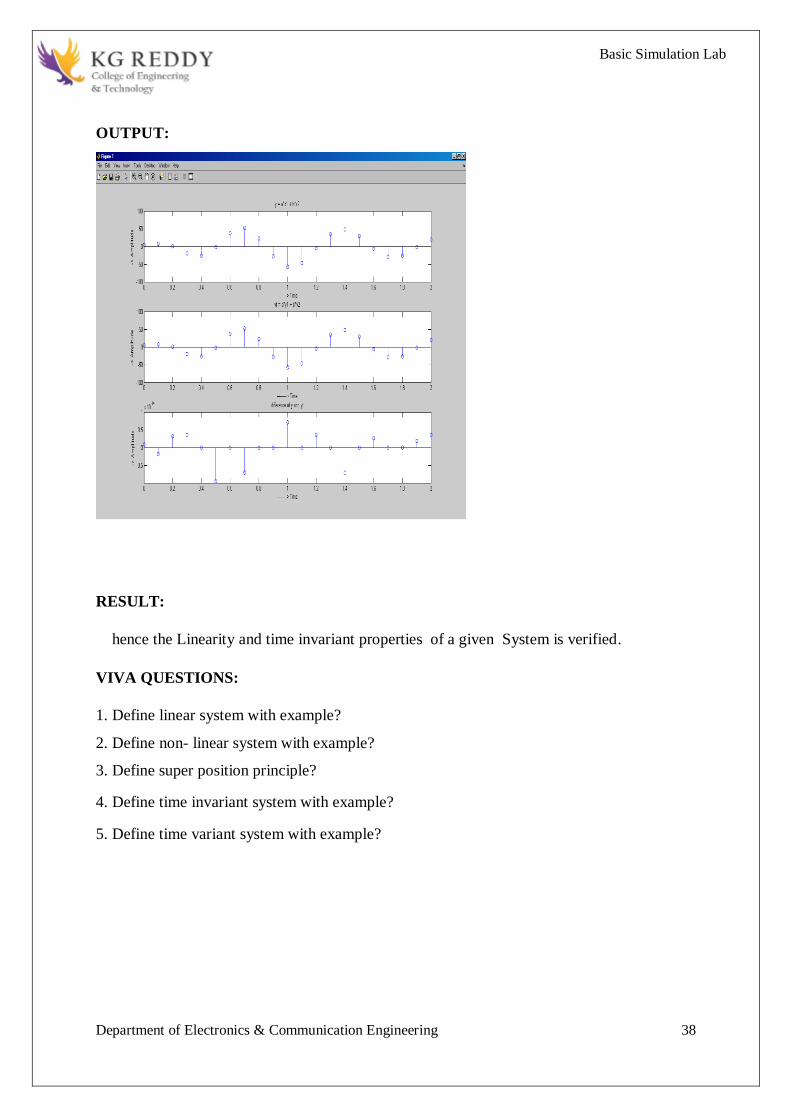
PROGRAM:

clc;

n=0:0.1:2;

a= -3; b= 5;

x1=cos(2*%pi*n);

x2=cos(3*%pi*n);

x=a*x1+b*x2;

ic=[0 0];

num=[2.2403 2.4908 2.2403];

den=[1 -0.4 0.75];

y1=filter (num, den, x1, ic);

y2=filter(num,den,x2,ic);

y=filter (num, den, x, ic);

yt=a*y1+b*y2;

d=y-yt;

subplot (3,1,1);

plot2d3 (n,y);

xlabel('---------> Time');

ylabel('-> Amplitude');

title('y = a*x1 + b*x2');

subplot(3,1,2);

plot2d3(n,yt);

xlabel('---------> Time');


title('yt = a*y1 + b*y2');

subplot(3,1,3);

plot2d3(n,d);

xlabel('---------> Time');


title('difference of y and yt');



OUTPUT:

RESULT:

hence the Linearity and time invariant properties of a given System is verified.

VIVA QUESTIONS:

1. Define linear system with example?

2. Define non- linear system with example?

3. Define super position principle?

4. Define time invariant system with example?

5. Define time variant system with example?



EXPERIMENT -8

COMPUTATION OF UNIT SAMPLE, UNIT STEP AND SINUSOIDAL

RESPONSE OF THE GIVEN LTI SYSTEM AND VERIFYING ITS

STABILITY

AIM: Write a program to compute the Unit sample, unit step and sinusoidal response of the given

LTI system and verifying its stability


THEORY:

A discrete time system performs an operation on an input signal based on predefined criteria

to produce a modified output signal. The input signal x(n) is the system excitation, and y(n) is

the system response. The transform operation is shown as,

If the input to the system is unit impulse i.e. x(n) = δ(n) then the output of the system is

known as impulse response denoted by h(n) where,

h(n) = T[δ(n)]

we know that any arbitrary sequence x(n) can be represented as a weighted sum of discrete

impulses. Now the system response is given by,

For linear system (1) reduces to

%given difference equation y(n)-y(n-1)+.9y(n-2)=x(n);



PROCEDURE:






PROGRAM:

// Impulse Response of an LTI system

clear all;

close all;

clc;

h = (-0.9).^[0:49];

subplot (2,2,1);

stem ([0:49],h,'filled');

xlabel('Samples');

ylabel('Amplitude');

title('h = (-0.9).^[0:49]');

u = ones(1);

subplot(2,2,2);

stem(u,'filled');

xlabel('Samples');


title('Impulse');

s = conv(u,h);

subplot(2,2,[3,4]);

stem([0:49],s(1:50));



xlabel('Samples');


title('Response for an impulse');

// Step Response of an LTI system:

clear all;

close all;

clc;

h = (-0.9).^[0:49];

subplot (2,2,1);

stem([0:49],h,'filled');

xlabel('Samples');


title('h = (-0.9).^[0:49]');

u = ones(1,50);

subplot(2,2,2);

stem([1:50],u,'filled');

xlabel('Samples');


title('Step');

s = conv(u,h);

subplot(2,2,[3,4]);

stem([0:49],s(1:50));

xlabel('Samples');


title('Response for a step');

// Sinusoidal Response of an LTI System:

clear all;

close all;

clc;

t = 1:0.04:2;

h = (-0.9).^t;

subplot(2,2,1);

stem(t,h,'filled');

xlabel('Samples');


title('h = (-0.9).^t');

u = sin(2*pi*t);

subplot(2,2,2);

stem(t,u,'filled');

xlabel('Samples');




title('Sine');

s = conv(u,h);

subplot(2,2,[3,4]);

stem([0:49],s(1:50));

xlabel('Samples');


title('Response for a sine');

// Stability of a given LTI System:

clear all;

close all;

clc;

n=0:0.1:20;

h= (0.5)*exp(-n);

sum=0;

for k=1:201

if abs(h(k))<10^(-6)

end

sum=sum+h(k);

end

stem(n,h);

disp('The summation value is ....:: ');sum

if sum > 5.0983e+008

disp('The System is unstable');

else

disp('The System is stable');

end;



OUTPUT:



The summation value is ....::

sum = 5.2542

The System is stable



RESULT: The Unit sample, unit step and sinusoidal response of the given LTI system is computed and its

stability verified. Hence all the poles lie inside the unit circle, so system is stable.

VIVA QUESTIONS:

1. What operations can be performed on signals and sequence?

2. Define causality and stability?

3. Define step response and impulse response of the system.

4. Define poles and zeros of the system?

5. What is the function of filter?



EXPERIMENT – 9

GIBBS PHENOMENON

AIM: Write a program to verify the Gibbs phenomenon.


THEORY:

The Gibbs phenomenon, the Fourier series of a piecewise continuously differentiable periodic

function behaves at a jump discontinuity. The n the approximated function shows amounts of

ripples at the points of discontinuity. This is known as the Gibbs Phenomena. partial sum of the

Fourier series has large oscillations near the jump, which might increase the maximum of the

partial sum above that of the function itself. The overshoot does not die out as the frequency

increases, but approaches a finite limit. The Gibbs phenomenon involves both the fact that Fourier

sums overshoot at a jump discontinuity, and that this overshoot does not die out as the frequency

increase.

PROCEDURE:






PROGRAM:

clc;

J= 500 //number of points

x=linspace(0,2*%pi, J);

f= sign(x); //returns array same size as x

kp=0.*x; //multiplies everything by x starting with 0

t=150

for k=1:2:t

kp=kp+(1/2)*sin(k*x)/k;

end

plot(x,kp)



OUTPUT:

RESULT:

In this , Gibbs phenomenon have been demonstrated using SCILAB

VIVA QUESTIONS:

1. Define Gibb’s Phenomenon?

2. What is the importance of Gibb’s Phenomenon?

3. What is Static and Dynamic System?

4.Define Fourier series ?

5. What is Causality Condition of the Signal?



EXPERIMENT -10

FINDING THE FOURIER TRANSFORM OF A GIVEN SIGNAL AND

PLOTTING ITS MAGNITUDE AND PHASE

SPECTRUM

AIM: Write a program to find the Fourier Transform of a given signal and plotting its magnitude

and phase spectrum.


THEORY:

Fourier Transform:

The Fourier transform as follows. Suppose that ƒ is a function which is zero outside of some

interval [−L/2, L/2]. Then for any T ≥ L we may expand ƒ in a Fourier series on the interval

[−T/2,T/2], where the "amount" of the wave e2πinx/T in the Fourier series of ƒ is given By

definition Fourier Transform of signal f(t) and inverse fourier transform is defined as

PROCEDURE:








PROGRAM:

clc ;

f=150 //(' enter the frequency in hertzs ');

Fs=2000 //('enter the samplinf freq in khz ')

Ts=1/(Fs);

N=128 //('enter the DFT sequence ');

n=[0:N-1]*Ts;

x=0.8*cos(2*%pi*f*n);

plot(n,x);

set(gca(),"grid",[1 1]);

data_bounds=([0 -1 ; 0.05 1]);

title(' cosine signal frequency ');

xlabel('time in n(sec) ');

ylabel(' amplitude');

Y=fft(x);

w=0:N-1;

figure;

Xmag=abs(Y);

subplot(2,1,1);

plot(w,Xmag);


title(' magnitude of fourier transform ');

xlabel(' frequency index w-------> ');

ylabel(' magnitude -----> ');

Xphase= atan(imag(Y),real(Y));

subplot(2,1,2);

plot(w,Xphase);


title(' phase of fourier transform ');

xlabel(' frequency index w-------> ');

ylabel(' phase -----> ');



OUTPUT:



RESULT:

Magnitude and phase spectrum of fourier transform of a given signal is plotted.

VIVA- VOCE QUESTIONS:

1. Define convolution property of Fourier transform?

2. What are the properties of Continuous-Time Fourier transform?

3. What is the sufficient condition for the existence of F.T?

4. Define the F.T of a signal?

5. What is the difference b/w F.T&F.S?



EXPERIMENT – 11

WAVEFORM SYNTHESIS USING LAPLACE TRANSFORMS

AIM: write a program to perform Wave form synthesis using Laplace Transforms

SOFTWARE REQUIRED: PC loaded with SCILAB Software

THEORY:

Bilateral Laplace transforms:

The Laplace transform of a signal f(t) can be defined as follows:

Inverse Laplace transform

The inverse Laplace transform is given by the following formula :

PROCEDURE:






PROGRAM:

clear all;

close all;

clc;

syms t w s

x=input ('Laplace Transform of a function ....:: ');

disp('is ......:: ');

xf=laplace(x)

disp('Inverse Laplace Transform of a function ...:: ');

disp('is ......:: ');



xt=ilaplace(xf)

OUTPUT:

Laplace Transform of a function ....:: cos(w*t)

is ......::

xf = s/(s^2+w^2)

Inverse Laplace Transform of a function ....::

is ......::

xt =cos(w*t)

RESULT:

Hence performed the waveform synthesis using laplace transform


1. Define Laplace-Transform?

2. What is the Condition for Convergence of the L.T?

3. What is the Region of Convergence (ROC)?

4. State the Shifting property of L.T?

5. State convolution Property of L.T?



EXPERIMENT -12

LOCATING POLES AND ZEROS IN S-PLANE & Z-PLANE

AIM: : Write the program for locating poles and zeros and plotting pole-zero maps in s-plane

and z-plane for the given transfer function.


THEORY:

Z-transforms

The Z-transform, like many other integral transforms, can be defined as either a one-sided or

two-sided transform.

Bilateral Z-transform

The bilateral or two-sided Z-transform of a discrete-time signal x[n] is the function X(z)

defined as

Unilateral Z-transform

Alternatively, in cases where x[n] is defined only for n ≥ 0, the single-sided or unilateral

Ztransform is defined as

In signal processing, this definition is used when the signal is causal.

The roots of the equation P(z) = 0 correspond to the 'zeros' of X(z)

The roots of the equation Q(z) = 0 correspond to the 'poles' of X(z)

Example:



PROGRAM:

clc;

clear all;

close all;

num = input('Enter the numerator coefficients.....:: ');

den = input('Enter the denominator coefficients.....:: ');

H = tf(num,den);

[p z]=pzmap(H);

disp('zeros at z= ');

disp(z);

disp('poles at p= ');

disp(p);

subplot(2,1,1);

pzmap(H);

title('pole zero map in s-domain ');

subplot(2,1,2);

zplane(num,den);

title('pole zero map in z-domain ');

OUTPUT:

Enter the numerator coefficients.....:: [1 0 -3]

Enter the denominator coefficients.....:: [1 -3 4]

zeros at z=

1.7321

-1.7321

poles at p=

1.5000 + 1.3229i

1.5000 - 1.3229i



RESULT:

Pole-zero maps are plotted in s-plane and z-plane for the given transfer function


1.Study the details of pzmap() and zplane() functions?

2. What are poles and zeros?

3. How you specify the stability based on poles and zeros?

4. Define S-plane and Z-plane?

5. Define transfer function of the system?



EXPERIMENT -13

GENERATION OF GAUSSIAN NOISE

AIM: Write the program for Generation of Gaussian noise (Real and Complex),

computation of its mean, M.S. value and its Skew, kurtosis, and PSD, probability

distribution function.


THEORY:

Gaussian noise is statistical noise that has a probability density function (abbreviated pdf) of the

normal distribution (also known as Gaussian distribution). In other words, the values the noise

can take on are Gaussian-distributed. It is most commonly used as additive white noise to yield

additive white Gaussian noise (AWGN).Gaussian noise is properly defined as the noise with a

Gaussian amplitude distribution. says nothing of the correlation of the noise in time or of the

spectral density of the noise. Labeling Gaussian noise as 'white' describes the correlation of the

noise. It is necessary to use the term "white Gaussian noise" to be correct. Gaussian noise is

sometimes misunderstood to be white Gaussian noise, but this is not the case.

PROCEDURE:






.PROGRAM:

clc;

clear all;

close all;

N= input(' Enter the number of samples ....:: ');

R1=randn(1,N);

M=mean(R1);

K=kurtosis (R1);



P=periodgram(R1);

V=var(R1);

x = psd(R1);

subplot(2,2,1);

plot(R1);

xlabel('Sample Number');


title('Normal [Gaussian] Distributed Random Signal');

subplot(2,2,2);

hist(R1);


ylabel('Total');

title('Histogram [Pdf] of a normal Random Signal');

subplot(2,2,[3,4]);

plot(x);



title('PSD of a normal Random Signal');

OUTPUT:



RESULT:

Hence Gaussian noise (Real and Complex) is generated and compute mean, M.S. value

and its Skew, kurtosis, and PSD, probability distribution function.


1 What is a noise and how many types of noises are there?

2. What is Gaussian noise?

3. What is correlation? How many types of correlation are there?

4. State Parseval’s energy theorem for a periodic signal?

5. What is Signum function?



EXPERIMENT -14

SAMPLING THEOREM VERIFICATION

AIM: - Write a program to Verify the sampling theorem.


THEORY:

Sampling Theorem:

A bandlimited signal can be reconstructed exactly if it is sampled at a rate atleast twice the

maximum frequency component in it." Figure 1 shows a signal g(t) that is bandlimited

Figure 1: Spectrum of band limited signal g(t)

The maximum frequency component of g(t) is fm. To recover the signal g(t) exactly from its

samples it has to be sampled at a rate fs ≥ 2fm. The minimum required sampling rate fs = 2fm is

called ' Nyquist rate

PROCEDURE:








PROGRAM:

clc;

clear all;

t=-5:.1:5;

T=4;

fm=1/T;

x=cos(2*pi*fm*t);

subplot(2,2,1);

plot(t,x);

xlabel('time');

ylabel('x(t)')

title('continous time signal')

grid;

n1=-2:1:2;

fs1=1.6*fm;

fs2=2*fm;

fs3=8*fm;

x1=cos(2*pi*fm/fs1*n1);

subplot(2,2,2);

stem(n1,x1);

xlabel('time');ylabel('x(n)')

title('discrete time signal with fs<2fm')

hold on

subplot(2,2,2);

plot(n1,x1)

grid;

n2=-3:1:3;


subplot(2,2,3);

stem(n2,x2);

xlabel('time');

ylabel('x(n)')

title('discrete time signal with fs=2fm')

hold on

subplot(2,2,3);

plot(n2,x2)

grid;

n3=-10:1:10;


subplot(2,2,4);

stem(n3,x3);

xlabel('time');

ylabel('x(n)')

title('discrete time signal with fs>2fm')

hold on

subplot(2,2,4);

plot(n3,x3)

grid;



OUTPUT:

RESULT:

Sampling theorem is verified.

VIVA-VOCE QUESTIONS:

1. State Parseval’s energy theorem for a periodic signal?

2. Define sampling Theorem?

3. What is Aliasing Effect?

4. What is under sampling?

5. What is over sampling?



EXPERIMENT -15

REMOVAL OF NOISE BY AUTO CORRELATION/CROSS

CORRELATION

AIM: Write the program for Removal of Noise by Auto Correlation/Cross Correlation.


THEORY:

Detection of a periodic signal masked by random noise is of great importance .The noise signal

encountered in practice is a signal with random amplitude variations. A signal is uncorrelated with

any periodic signal.

Detection of noise by Auto-Correlation:

S(t)=Periodic Signal (Transmitted) , mixed with a noise signal n(t).

Then f(t) is received signal is [s(t ) + n(t) ]

Let Qff(T) =Auto Correlation Function of f(t)

Qss(t) = Auto Correlation Function of S(t)

Qnn(T) = Auto Correlation Function of n(t)

T/2

Qff(T)= Lim 1/T ∫ f(t)f(t-T) dt

T--∞ -T/2

T/2

= Lim 1/T ∫ [s(t)+n(t)] [s(t-T)+n(t-T)] dt

T--∞ -T/2

=Qss(T)+Qnn(T)+Qsn(T)+Qns(T)

The periodic signal s(t) and noise signal n(t) are uncorrelated

Qsn(t)=Qns(t)=0 ;

Then Qff(t)=Qss(t)+Qnn(t)

The Auto correlation function of a periodic signal is periodic of the same frequency and the Auto

correlation function of a non periodic signal is tends to zero for large value of T since s(t) is a



periodic signal and n(t) is non periodic signal so Qss(T) is a periodic where as a Qnn(T) becomes

small for large values of T Therefore for sufficiently large values of T Qff(T) is equal to Qss(T).

PROCEDURE:






PROGRAM:

clear all;

close all;

clc;

t=0:0.1:pi*4;

s=sin(t);

k=2;

subplot(3,1,1);

plot(s);

xlabel('---> time');


title('Original signal');

n=rand(1,126);

f=s+n;

subplot(3,1,2);

plot(f);



title('Signal+noise');

as=xcorr(s,s);

subplot(3,1,3);

plot(as);



title('auto correlation s(t)');

figure;

an=xcorr(n,n);

subplot(3,1,1)



plot(an);



title('auto correlation n(t)');

af=xcorr(f,f);

subplot(3,1,2)

plot(af);



title('auto correlation f(t)');

hh=as+an;

subplot(3,1,3)

plot(hh);



title('addition of s(t) and n(t)');

OUTPUT:



RESULT:

Removal of noise using autocorrelation is performed.


1. Define Auto correlation function?

2. What are the Different types of noise signals?

3. Define cross correlation function?

4. What is Signum function?

5. What is Static and Dynamic System?



EXPERIMENT -16

EXTRACTION OF PERIODIC SIGNAL MASKED BY NOISE USING

CORRELATION

AIM: write the program for Extraction of periodic signal masked by noise using correlation


THEORY:

A signal is masked by noise can be detected either by correlation techniques or by filtering.

Actually, the two techniques are equivalent. The correlation technique is a measure of extraction

of a given signal in the time domain whereas filtering achieves exactly the same results in

frequency domain.

PROCEDURE:






PROGRAM:

clear all;

close all;

clc;

N= input('Enter the number of samples .....:: ');

M= input('Enter the number of cycles .....:: ');

h=1/N;

x=0:h:M;

y=cos(3*pi*x);

subplot(4,1,1);

plot(x,y);





title('Original signal');

w=rand(1,M*N+1);

subplot(4,1,2);

plot(x,w);



title('Noise');

k=y+w;

subplot(4,1,3);

plot(x,k);



title('Signal+noise');

m=xcorr(k);

subplot(4,1,4)

plot(x,0.01*m(1:M*N+1));



title('Recovered signal');

OUTPUT:

Enter the number of samples .....:: 100

Enter the number of cycles .....:: 4



RESULT:

Periodic signal is extracted by using correlation.


1. State the relationship between PSD and ACF?

2. What is the integration of ramp signal?

3. Difference between vectors and signals?

4. Define PSD?

5. Define Hilbert transforms?



EXPERIMENT -17

VERIFICATION OF WIENER-KHINCHIN RELATION

AIM: Write a program to Verify wiener-khinchin relation


THEORY:

The wiener-khinchin theorem states that the power spectral density of a wide sense stationary

random process is the flourier transform of the corresponding autocorrelation function.

PROCEDURE:






PROGRAM:

clc

clear all;

t=0:0.01:2*pi;

x=sin(2*t);

subplot(3,2,1);

plot(x);

au=xcorr(x,x);

Subplot (3,2,2);

plot (au);



v=fft(au);

subplot(3,2,3);

plot(abs(v));

fw=fft(x);

subplot(3,2,4);

plot(fw);

fw2=(abs(fw)).^2;

subplot(3,2,5);

plot(fw2);

OUTPUT:



RESULT:

wiener-khinchin relation is verified.


1. What is mean wiener-khinchine relation?

2. Define fourier transform and its inverse?

3. What is the difference b/w convolution and correlation?

4. What is the importance of power spectrum?

5. What is the importance of correlation?



EXPERIMENT -18

CHECKING A RANDOM PROCESS FOR STATIONARITY IN WIDE

SENSE

AIM: Write a program for Checking a Random Process for Stationary in Wide Sense

SOFTWARE REQUIRED: PC loaded with SCILAB Software

THEORY:

The concept of stationarity plays an important role in solving practical problems involving

random processes. Just like time-invariance is an important characteristics of many deterministic

systems, stationarity describes certain time-invariant property of a class of random processes.

Stationarity also leads to frequency-domain description of a random process.

Strict-sense Stationary Process

A random process is called strict-sense stationary (SSS) if its probability structure is

invariant with time. In terms of the joint distribution function, is called SSS if

Thus, the joint distribution functions of any set of random variables does not

depend on the placement of the origin of the time axis. This requirement is a very strict. Less strict

form of stationarity may be defined.



PROCEDURE:






PROGRAM:

clear all;

close all;

clc;

syms x

z = input('Enter the function ..... :: ');

Max = input('Max limit ....:: ');

Min = input('Min limit ....:: ');

mean_value = int(z,Min,Max)

y = subs(z,x,x+5);

Auto_correlation = int(z*y,Min,Max)

disp('If the mean value is constant .....');

disp('and');

disp('Auto Correlation is not a function of x variable ....');

disp('then ');

disp('The Random Process is Wide Sense stationary.');

OUTPUT:

Enter the function ..... :: 10*cos(10*x + 100)

Max limit ....:: 2*pi

Min limit ....:: 0

mean_value =0

Auto_correlation =100*cos(50)*pi

If the mean value is constant.....

and

Auto Correlation is not a function of x variable ....

then

The Random Process is Wide Sense stationary.



RESULT:

Hence checked the wide sense stationarity random process


1. Define random process?

2. Give the types of random process?

3. Give the importance of random process?

4. Define strict-sense stationarity random process?

5. Define wide-sense stationarity random process?

experiment- 1 basic operations on...

Documents