EXPERIMENT 4 The Oscilloscope

Objectives 1) Explain the operation or effect of each control on a simple oscilloscope.

2) Display an unknown sinusoidal electrical signal on an oscilloscope and measure its amplitude and frequency.

Introduction To measure an electrical voltage you would use a voltmeter. But what happens if the electrical voltage you want to measure is varying rapidly in time? The voltmeter display may oscillate rapidly preventing you making a good reading, or it may display some average of the time varying voltage. In this case, an oscilloscope can be used to observe, and measure, the entire time-varying voltage, or "signal". The oscilloscope places an image of the time-varying signal on the screen of a cathode ray tube (CRT) allowing us to observe the shape of the signal and measure the voltage at different times. If the signal is periodic (it repeats itself over and over) as is often the case, we can also measure the frequency, the rate of repeating, of the signal. What the Oscilloscope Does The oscilloscope plots voltage as a function of time.

Figure 1

There are two types of voltages AC and DC. AC (derived from ALTERNATING CURRENT) indicates a voltage, the magnitude of which varies as a function of time. An AC signal is shown in Figure 1. In contrast, DC (derived from DIRECT CURRENT) indicates a voltage whose magnitude is constant in time. The voltage is on the vertical (y) axis and the time is on the horizontal (x) axis. A constant voltage (DC) shows up as a flat horizontal line. The scope has controls to make the x and y scales larger or smaller. These act like the controls for magnification on a microscope. They don’t change the actual voltage any more than magnification makes a cell on the microscope slide bigger; they just let us see small details more easily. There are also controls to shift the center points of the voltage scales. These “offset” knobs are like the controls to move the stage of the microscope to look at different parts of a sample. You will learn about other adjustments in the course of the lab. The Oscilloscope Experiment In this experiment you will familiarize yourself with the use of an oscilloscope. Using a signal generator you will produce various time varying voltages (signals) which you will input into the oscilloscope for analysis. There are two main quantities which can be measured with the aid of an oscilloscope that characterize any periodic AC signal. The first is the peak-to-peak voltage (Vpp), which is defined as the voltage difference between the time-varying signal’s highest and lowest voltage (see the square wave shown in Figure 2). The second is the frequency of the time-varying signal (f), defined by

f =1T

f is the frequency in Hz and T is the period in seconds (the period is also shown in Figure 2). Sometimes the angular frequency ω in rad/sec is used instead of the frequency f in Hz. They are related by:

fπω 2=

The form of an AC signal is:

DCVftV +)2sin(0 π where, VDC is a constant DC offset, that shifts the sine wave up or down. The form of an AC signal with no DC offset is: )2sin(0 ftV π

The amplitude, V0, is related to the peak-to-peak voltage Vpp of the signal by:

Vpp = 2V0

Figure 2

How the Oscilloscope Works An oscilloscope contains a cathode ray tube (CRT), in which the deflection of an electron beam that falls onto a phosphor screen is directly proportional to the voltage applied across a pair of parallel deflection plates. A measurement of this deflection yields a measurement of the applied voltage. The oscilloscope can be used to display and measure rapidly varying electrical phenomena. The internal subsystems of the oscilloscope are shown in Figure 3a and the front panel of the oscilloscope is shown in Figure 3b. To see the front panel of the oscilloscope in more detail, open the pdf file for this lab on the course web page and use Adobe’s magnify option.

Figure 3a

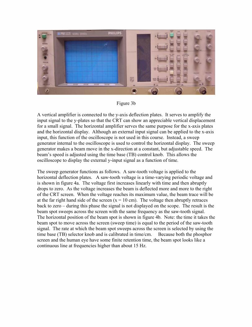
Figure 3b

A vertical amplifier is connected to the y-axis deflection plates. It serves to amplify the input signal to the y-plates so that the CRT can show an appreciable vertical displacement for a small signal. The horizontal amplifier serves the same purpose for the x-axis plates and the horizontal display. Although an external input signal can be applied to the x-axis input, this function of the oscilloscope is not used in this course. Instead, a sweep generator internal to the oscilloscope is used to control the horizontal display. The sweep generator makes a beam move in the x-direction at a constant, but adjustable speed. The beam’s speed is adjusted using the time base (TB) control knob. This allows the oscilloscope to display the external y-input signal as a function of time. The sweep generator functions as follows. A saw-tooth voltage is applied to the horizontal deflection plates. A saw-tooth voltage is a time-varying periodic voltage and is shown in figure 4a. The voltage first increases linearly with time and then abruptly drops to zero. As the voltage increases the beam is deflected more and more to the right of the CRT screen. When the voltage reaches its maximum value, the beam trace will be at the far right hand side of the screen (x = 10 cm). The voltage then abruptly retraces back to zero – during this phase the signal is not displayed on the scope. The result is the beam spot sweeps across the screen with the same frequency as the saw-tooth signal. The horizontal position of the beam spot is shown in figure 4b. Note: the time it takes the beam spot to move across the screen (sweep time) is equal to the period of the saw-tooth signal. The rate at which the beam spot sweeps across the screen is selected by using the time base (TB) selector knob and is calibrated in time/cm. Because both the phosphor screen and the human eye have some finite retention time, the beam spot looks like a continuous line at frequencies higher than about 15 Hz.

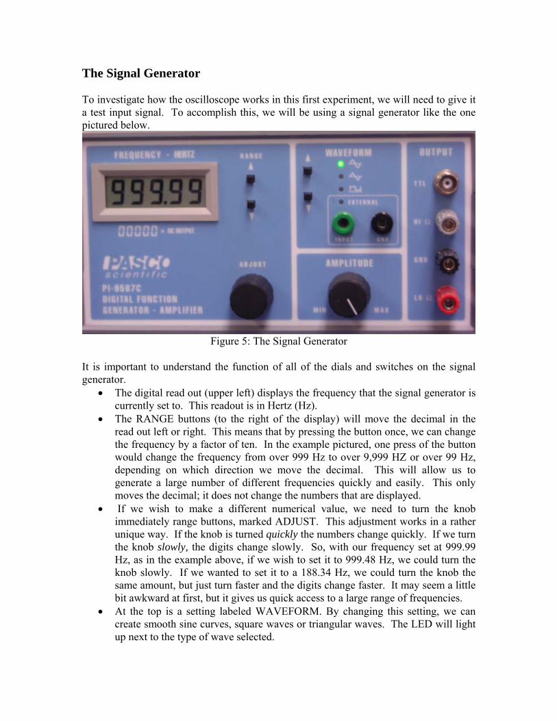
The Signal Generator To investigate how the oscilloscope works in this first experiment, we will need to give it a test input signal. To accomplish this, we will be using a signal generator like the one pictured below.

Figure 5: The Signal Generator

It is important to understand the function of all of the dials and switches on the signal generator.

• The digital read out (upper left) displays the frequency that the signal generator is currently set to. This readout is in Hertz (Hz).

• The RANGE buttons (to the right of the display) will move the decimal in the read out left or right. This means that by pressing the button once, we can change the frequency by a factor of ten. In the example pictured, one press of the button would change the frequency from over 999 Hz to over 9,999 HZ or over 99 Hz, depending on which direction we move the decimal. This will allow us to generate a large number of different frequencies quickly and easily. This only moves the decimal; it does not change the numbers that are displayed.

• If we wish to make a different numerical value, we need to turn the knob immediately range buttons, marked ADJUST. This adjustment works in a rather unique way. If the knob is turned quickly the numbers change quickly. If we turn the knob slowly, the digits change slowly. So, with our frequency set at 999.99 Hz, as in the example above, if we wish to set it to 999.48 Hz, we could turn the knob slowly. If we wanted to set it to a 188.34 Hz, we could turn the knob the same amount, but just turn faster and the digits change faster. It may seem a little bit awkward at first, but it gives us quick access to a large range of frequencies.

• At the top is a setting labeled WAVEFORM. By changing this setting, we can create smooth sine curves, square waves or triangular waves. The LED will light up next to the type of wave selected.

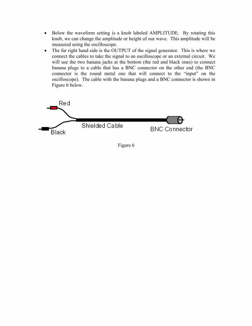
• Below the waveform setting is a knob labeled AMPLITUDE. By rotating this knob, we can change the amplitude or height of our wave. This amplitude will be measured using the oscilloscope.

• The far right hand side is the OUTPUT of the signal generator. This is where we connect the cables to take the signal to an oscilloscope or an external circuit. We will use the two banana jacks at the bottom (the red and black ones) to connect banana plugs to a cable that has a BNC connector on the other end (the BNC connector is the round metal one that will connect to the “input” on the oscilloscope). The cable with the banana plugs and a BNC connector is shown in Figure 6 below.

Figure 6

WORKSHEET The Oscilloscope

Experiment 4

Name_________________________

Lab Partner____________________

Section________________________

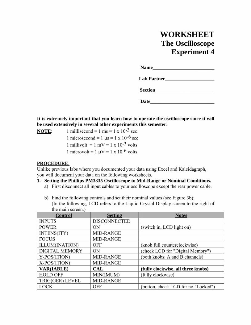
Date__________________________ It is extremely important that you learn how to operate the oscilloscope since it will be used extensively in several other experiments this semester! NOTE: 1 millisecond = 1 ms = 1 x 10-3 sec 1 microsecond = 1 μs = 1 x 10-6 sec 1 millivolt = 1 mV = 1 x 10-3 volts 1 microvolt = 1 μV = 1 x 10-6 volts PROCEDURE: Unlike previous labs where you documented your data using Excel and Kaleidagraph, you will document your data on the following worksheets. 1. Setting the Phillips PM3335 Oscilloscope to Mid-Range or Nominal Conditions.

a) First disconnect all input cables to your oscilloscope except the rear power cable. b) Find the following controls and set their nominal values (see Figure 3b): (In the following, LCD refers to the Liquid Crystal Display screen to the right of

the main screen.) Control Setting Notes

INPUTS DISCONNECTED POWER ON (switch in, LCD light on) INTENS(ITY) MID-RANGE FOCUS MID-RANGE ILLUM(INATION) OFF (knob full counterclockwise) DIGITAL MEMORY ON (check LCD for "Digital Memory") Y-POS(ITION) MID-RANGE (both knobs: A and B channels) X-POS(ITION) MID-RANGE VAR(IABLE) CAL (fully clockwise, all three knobs) HOLD OFF MIN(IMUM) (fully clockwise) TRIG(GER) LEVEL MID-RANGE LOCK OFF (button, check LCD for no "Locked")

c) Now press the AUTO SET button. This will automatically reset the internal electronics of the oscilloscope to reasonable nominal settings. Your oscilloscope should now display a horizontal line across the screen. If not, go back and recheck that each control is in the nominal position. If the horizontal line still does not appear ask your instructor for help. If you ever get lost later in the lab, you can return to the nominal settings. (The AUTO SET button does not necessarily give you the best configuration for your particular measurement; it gives nominal settings which are a good starting point. You will then use manual adjustments to customize the setup.)

2. Adjustments

a) Adjust the FOCUS and INTENSITY controls for a sharp and moderately bright line.

b) Rotate the Y POS knob associated with the A-Channel (top knob) and move the horizontal line up and down on the screen. Set the line near the middle of the screen.

c) Set the display to Channel B: keep pressing the A/B button until you see "B" (and no "A") indicated on the LCD. You can now adjust the Y POS knob of the B-Channel. Set the line near the middle of the screen.

d) Set the display to both Channel A and B simultaneously: "A" and "B" indicated on the LCD.

e) Rotate the Y POS knobs for both channels A and B. Notice that the signal moves up and down on the screen and note the independence of the two controls. Reset both to the center of the screen and then set the display for Channel A only.

3. Digital and Analog The oscilloscope can be operated in either digital or analog mode. Although you will use the digital side of the oscilloscope in all of the subsequent labs, we will briefly use the analog side of the oscilloscope first to help you understand how a signal is displayed on the oscilloscope. You can switch between the digital and analog modes by pressing the DIGITAL MEMORY button. In analog mode the trace comes on the screen directly from the input (after some amplification or attenuation). The voltage of the input signal is given by the vertical displacement of the trace on the screen. To measure the voltage in analog mode, you need to know the sensitivity setting of the scope. The sensitivity V/mV is changed using the switch labeled A for signals on channel A and the switch labeled B for signals on channel B. The sensitivity setting is displayed on the LCD screen. The voltage and its uncertainty are then calculated by:

)()/()( cmHeightcmvoltsySensitivitvoltsV ×=

and

Height(Height) δδ VV =

The height is measured using the grid on the CRT’s screen. Each of the 80 squares which make up the grid is 1.0 cm on a side. You should make a reasonable estimate of the uncertainty in the height when making a measurement in analog mode. In digital mode, the oscilloscope automatically digitizes the input voltage. It quickly (up to forty million times per second) reads the input signal and stores its value in Volts in its electronic memory. The contents of the memory are then displayed on the screen (at 100,000 times per second or less). You can then calculate the voltage using the same method as you would in analog mode, or you can use the screen cursors (see oscilloscope cursor appendix for outline) to help you to read the voltage directly off of the screen. You will use both methods in this experiment. 4. View the oscilloscope without an input signal in analog mode Turn on the oscilloscope and make sure it is in analog mode. Use the switch labeled TB to set the time base to its largest possible value and record in the data table below. The time base setting is displayed on the LCD screen. You should now see the beam move across the CRT screen. Using the time base, calculate how long it takes the beam to move across the screen. Also, estimate the uncertainty in the distance the beam travels (δ distance) across the screen and use it to calculate the uncertainty in your calculated time. In addition, directly measure the time the beam takes to move across the screen using a clock, watch or timer. Estimate the uncertainty in this time.

t = time base(seconds/cm) × distance(cm)

distance(distance) δδ tt =

TABLE 1

Time base setting

Distance traveled

±

Time (calculated)

±

Time (measured)

±

Question 1: Are the two times in Table 1 consistent? What is the meaning of this result?

5. View the input signal from the signal generator. The signal generator produces a signal which is simply an electric voltage which varies with time. We will be using sine-wave signals in this lab. Here, the voltage varies in time like a sine-wave oscillating between a positive and negative voltage at a particular frequency. Attach the output of the signal generator to the channel A input of the oscilloscope using a cable with banana jacks at one end and a BNC connector at the other. The signal generator produces voltage signals of different frequencies and peak-to-peak voltages. In order to use the signal generator effectively, we will have to learn something about its operation. Set the knobs on the signal generator initially as indicated below: FREQUENCY = 60.000 WAVEFORM = smooth sine wave AMPLITUDE = Approximately the Middle Change the oscilloscope to digital mode. Press the AUTO SET button on the oscilloscope. Adjust the sensitivity setting (A) so that the peak to peak signal fills most of the oscilloscope’s screen, without extending above or below the grid. Also, adjust the time base so that one period of the signal fills most of the grid. NOTE: making these changes to the sensitivity and time base does not change the voltage or period of the signal; it only changes the scale the oscilloscope uses to display the signal. Sketch the signal displayed on the oscilloscope on the grid below.

Using the oscilloscope, estimate the period and peak to peak voltage (Vpp) of the signal. Recall, the period is the time required for the signal to repeat. Include a reasonable uncertainty for each of these quantities. Also, from your measurement of the period, calculate the frequency of the signal measured by the oscilloscope. The uncertainty in

the frequency is given by: TTff δδ = , where T and δT are the period and the uncertainty

in the period in seconds. Record these measurements in Table 2.

Table 2

Voltage sensitivity setting

Peak to peak height of signal on the CRT screen

±

Vpp

±

Time base setting

Distance for the signal to repeat on the CRT screen

±

Period

±

Frequency

±

Show your calculations for Table 2 here: Question 2: Is the frequency measured on the oscilloscope consistent with the frequency set on the function generator?

6. Using the cursors with the digital oscilloscope. Inspect the CRT screen. If there is no writing at the bottom of the screen, press one of the blue keys just below the screen. If there is some writing and one of the soft keys has RETURN written above it, press the RETURN soft key and keep pressing it until RETURN is no longer visible. This returns you to the highest menu level. You should now see:

CURSORS SETTINGS INTF TEXT_OFF at the bottom of the CRT screen. You can use these soft keys to help you measure voltages, times, periods and frequencies of input signals. Appendix 1 to this experiment is an outline of the soft key structure. a. Measuring peak to peak voltage. We will use the soft keys to move the screen cursors (reference lines) to read voltages and times from the CRT screen. Press the CURSORS soft key. Press the MODE soft key to set up the cursors you wish to use. Press the V-CURS ON/OFF soft key to toggle the two horizontal cursors on and off – you want these on to measure voltage. Press the RETURN soft key to return to the main cursors menu. Press the V-CTRL soft key to control the two voltage cursors. Use the ↑ REF ↓ soft keys to move the bottom cursor up and down. Use the ↑Δ↓ soft keys to move the top cursor up and down. These two cursors are used to measure the peak to peak voltage of the input signal. The displayed voltage is the voltage difference between these two cursors; you move these cursors to make a measurement. To estimate the uncertainty in this measurement, use two clicks, or if the trace is larger than two clicks use the width of the trace. Measure the peak to peak voltage of your signal.

Vpp = ______ ± _____ Question 3: Does the peak to peak voltage measured using the cursors agree with the peak to peak voltage you recorded in Table 2? Using the sensitivity adjustment, you can change the height of the trace displayed on the screen without changing the actual input voltage. Change the sensitivity using the button labeled A on the oscilloscope. Re-adjust the cursors and measure the peak to peak voltage.

Question 4: Did changing the voltage sensitivity on the oscilloscope change the peak-to-peak voltage? Explain. Change the sensitivity back to its previous setting. The VAR knob varies the sensitivity in a continuous way, which cannot be interpreted by the electronics. Move the A VAR knob away from the full-right CAL position and observe what happens to the trace. Notice on the CRT a voltage is no longer displayed. It should now only tell you how many divisions (cm) apart the cursors are placed. Also, on the LCD display next to the voltage sensitivity you should see a blinking “>” – this means the actual voltage sensitivity is something greater than the value indicated on the LCD screen. When using the oscilloscope, it is very important that all three of the VAR knobs are set to the full-clockwise CAL position. Return the knob to the CAL position. b. Frequency measurement The digital mode of the oscilloscope can be used to measure the period and frequency of a signal. As with the peak to peak voltage measurements you can use the soft keys to help you measure these values. Now, you will use the T-cursors. Go to the MODE menu and use the T-CURS/ON/OFF soft key to turn on the two vertical cursors. Then go to the T-CTRL menu to set the location of your cursors. Use the →← REF and →Δ← soft keys to set the location of vertical cursors to correspond to one period of the input signal. At the top of the CRT screen you should see “Δt=” and “1/Δt=” corresponding to the period and the frequency of your signal. Period = ________±______ Frequency = ________±______ Question 5: Does the frequency measured using the cursors agree with the frequency you recorded in Table 2? Change the time base and re-measure the frequency.

Question 6: Did changing the time base change the frequency of the signal? Explain. Return the time base to its previous setting. 7. The features on the signal generator.

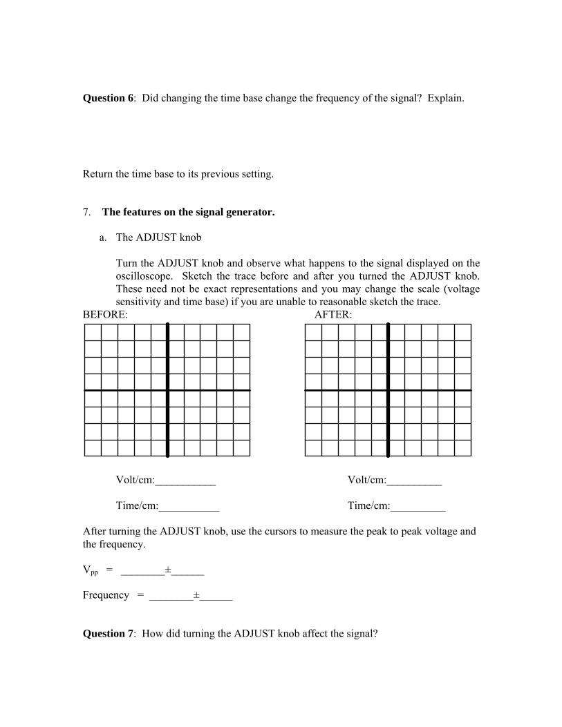
a. The ADJUST knob Turn the ADJUST knob and observe what happens to the signal displayed on the oscilloscope. Sketch the trace before and after you turned the ADJUST knob. These need not be exact representations and you may change the scale (voltage sensitivity and time base) if you are unable to reasonable sketch the trace.

BEFORE: AFTER:

Volt/cm:___________ Volt/cm:__________ Time/cm:___________ Time/cm:__________ After turning the ADJUST knob, use the cursors to measure the peak to peak voltage and the frequency. Vpp = ________±______ Frequency = ________±______ Question 7: How did turning the ADJUST knob affect the signal?

b. The RANGE setting Push one of the two RANGE buttons and observe what happens to the signal displayed on the oscilloscope. Sketch the trace before and after you pushed the RANGE. These need not be exact representations and you may change the scale (voltage sensitivity and time base) if you are unable to reasonable sketch the trace.

BEFORE: AFTER:

Volt/cm:___________ Volt/cm:__________ Time/cm:___________ Time/cm:__________ After pushing the RANGE button, use the cursors to measure the peak to peak voltage and the frequency. Vpp = ________±______ Frequency = ________±______ Question 8: How did turning the ADJUST knob affect the signal?

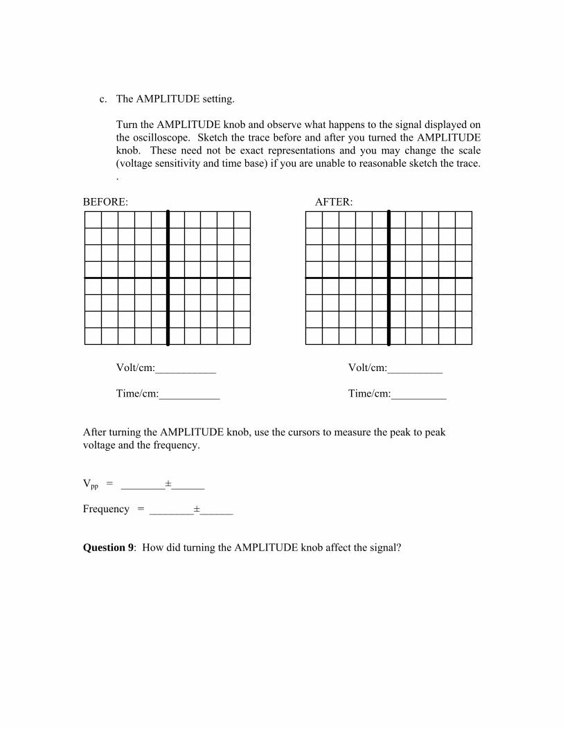
c. The AMPLITUDE setting.

Turn the AMPLITUDE knob and observe what happens to the signal displayed on the oscilloscope. Sketch the trace before and after you turned the AMPLITUDE knob. These need not be exact representations and you may change the scale (voltage sensitivity and time base) if you are unable to reasonable sketch the trace. .

BEFORE: AFTER:

Volt/cm:___________ Volt/cm:__________ Time/cm:___________ Time/cm:__________ After turning the AMPLITUDE knob, use the cursors to measure the peak to peak voltage and the frequency. Vpp = ________±______ Frequency = ________±______ Question 9: How did turning the AMPLITUDE knob affect the signal?

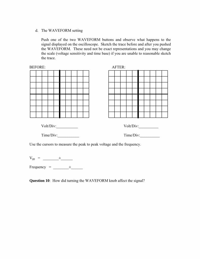
d. The WAVEFORM setting

Push one of the two WAVEFORM buttons and observe what happens to the signal displayed on the oscilloscope. Sketch the trace before and after you pushed the WAVEFORM. These need not be exact representations and you may change the scale (voltage sensitivity and time base) if you are unable to reasonable sketch the trace.

BEFORE: AFTER:

Volt/Div:___________ Volt/Div:__________ Time/Div:___________ Time/Div:__________ Use the cursors to measure the peak to peak voltage and the frequency. Vpp = ________±______ Frequency = ________±______ Question 10: How did turning the WAVEFORM knob affect the signal?

8. Signal triggering Most signals you will use the oscilloscope to view will be displayed such that you will not be able to see the beam spot, it will only appear as a trace, or curve. The time corresponding to the width of the screen will be very short, so you will want each trace to start in the same location. Otherwise, the signal will appear very erratic and it will be extremely difficult to make any measurements. The trigger lets the oscilloscope know where it should start its trace. If it is set properly, the signal will start in the same place for each successive sweep. For example, say you wanted to view an 8.0 V peak-to-peak signal; you could set the trace to start when the voltage exceeded +1.0 V. The scope will then start each trace at the same point of the signal; the rapid superposition of identical traces appears as a single trace to your eye. On the P-P setting, the trigger is a threshold voltage from the input signal. The threshold voltage is adjusted using the trigger level knob, but cannot be adjusted beyond the peak to peak limits of the input signal. When the input signal exceeds this threshold voltage, the oscilloscope starts its trace. If P-P is not displayed on the LCD screen, push the TRIG COUPL button a few times until you can see it. Turn the trigger level knob all the way to the left. Make sure you can see the start of the trace near the left hand edge of the screen. If it is not visible, use the X-POS knob to adjust its position. While watching the start of the trace, turn the knob to the right. Question 11: What happens to the left hand edge (start) of the trace as you turn the knob? Sometimes it is necessary to use the DC trigger setting instead of the P-P setting. It is possible to have the DC trigger set beyond the range of the signal you wish to view. As with the P-P setting, the oscilloscope will start its next trace once the threshold voltage is exceeded. Turn the TRIGGER LEVEL knob to the middle of its range. Then push the TRIG COUPL button until you see DC on the LCD (DC should appear close to the position where you previously saw P-P). Rotate the TRIGGER LEVEL knob to the right and observe what happens. Slowly rotate the knob back to the left until the trace becomes stable. The starting voltage of your trace is the threshold voltage. Question 12: How does this threshold voltage compare to the peak voltage of your input signal?

Set the TRIG COUPL button back to P-P and adjust the TRIG LEVEL knob so that the signal starts on the horizontal axis. Hint for the future: if you have trouble triggering on a signal, try using a higher voltage sensitivity (smaller V/cm) setting. 9. Measurement of an Unknown Sinusoidal Signal: Measure the frequency and Vpp for the mystery signal from the white box. Here you will connect the output of on unknown box directly to the oscilloscope. You will not need the signal generator. Be sure to turn on the power supply connected to the unknown box. White Box I.D. = ___________ Vpp = _______________±____________ Volts Frequency = ___________±___________ Hz 10. Additional questions Question 13: The diagram below shows a signal on the CRT screen of an oscilloscope. Sketch the appearance of the trace if the voltage sensitivity setting on the oscilloscope is increased by a factor of 2. Original display

Sensitivity doubled

Question 14: The voltage sensitivity is returned to its original setting, and then the time base is halved. Sketch the appearance of the trace after the time base has been decreased by a factor of 2. Original signal

Time base halved

Question 15: If you wish to measure the frequency of the signal more accurately, which trace should you use (original or with the time base halved)? Why? Question 16: Suppose you have an unknown input signal. Briefly describe the steps you would take to view the signal appropriately and to make measurements of the frequency, period, and peak to peak voltage.