experimental analysis of dynamic all pairs shortest path
TRANSCRIPT

Experimental Analysis of Dynamic
All Pairs Shortest Path Algorithms ∗
Camil Demetrescu † Giuseppe F. Italiano ‡
Abstract
We present the results of an extensive computational study on dynamic algorithmsfor all pairs shortest path problems. We describe our implementations of the recentdynamic algorithms of King and of Demetrescu and Italiano, and compare themto the dynamic algorithm of Ramalingam and Reps and to static algorithms onrandom, real-world and hard instances. Our experimental data suggest that some ofthe dynamic algorithms and their algorithmic techniques can be really of practicalvalue in many situations.
1 Introduction
In this paper we consider fully dynamic algorithms for all pairs shortest path problems.Namely, we would like to maintain information about shortest paths in a weighted di-rected graph subject to edge insertions, edge deletions and edge weight updates. Thisseems an important problem on its own, and it finds applications in many areas (see,e.g., [25]), including transportation networks, where weights are associated with traf-fic/distance; database systems, where one is often interested in maintaining distance re-lationships between objects; data flow analysis and compilers; document formatting; andnetwork routing [11, 23, 24].
This problem was first studied in 1967 [21, 22], but the first fully dynamic algorithmsthat in the worst case were provably faster than recomputing the solution from scratch wereproposed only twenty years later. We recall here that the all pairs shortest path problemcan be solved in O(mn+n2 log n) worst-case time with Dijkstra’s algorithm and Fibonacciheaps [9, 12], where m is the number of edges and n is the number of nodes. Since m
∗This work has been partially supported by the IST Programme of the EU under contract n. IST-1999-14.186 (ALCOM-FT), by the Italian Ministry of University and Research (Project “ALINWEB:Algorithmics for Internet and the Web”). A preliminary version of this paper was presented at the 15thAnnual ACM-SIAM Symposium on Discrete Algorithms (SODA’04), New Orleans, LA. January 2004.
†Dipartimento di Informatica e Sistemistica, Universita di Roma “La Sapienza”, Roma, Italy. Email:[email protected]. URL: http://www.dis.uniroma1.it/~demetres.
‡Dipartimento di Informatica, Sistemi e Produzione, Universita di Roma “Tor Vergata”, Roma, Italy.Email: [email protected]. URL: http://www.info.uniroma2.it/~italiano.
1

can be as high as Θ(n2), this is Θ(n3) in the worst case. In 1999 King [19] presented afully dynamic algorithm for maintaining all pairs shortest paths in directed graphs withpositive integer weights less than C: the running time of her algorithm is O(n2.5
√C log n )
per update and O(1) per query. Demetrescu and Italiano [7] showed how to maintain allpairs shortest paths on directed graphs with real-value edge weights that can take at most
S different values: their time bound is O(n2.5√
S log3 n ) per update and O(1) per query. In2003, the same authors [8] presented a fully dynamic shortest paths algorithm that requiresO(n2 · log3 n) time per update and constant time per query. This bound has been recentlyimproved to O(n2(log n + log2(m/n))) amortized time per update by Thorup [28].
Our Results.
The objective of this paper is to advance our knowledge on dynamic shortest path algo-rithms by following up the recent theoretical progress of King [19] and of Demetrescu andItaliano [8] with a thorough empirical study. In particular, we present and experimentwith efficient implementations of the dynamic shortest path algorithms described in thosepapers. We do not consider here the algorithm by Thorup [28], since preliminary inves-tigations suggest that this improvement is mainly of theoretical interest. Our empiricalanalysis shows that some of the dynamic algorithms and their techniques can be really ofpractical value in many situations. Indeed, we observed that in practice their speed upis much higher than the one predicted by theoretical bounds: they can be even two tofour orders of magnitude faster than repeatedly computing a solution from scratch with astatic algorithm. Furthermore, our work may shed light on the relative behavior of someimplementations on different test sets and on different computing platforms: this mightbe helpful in identifying the most suitable dynamic shortest path code for different appli-cation scenarios. As a side result of our experimental work, we propose also a new staticalgorithm, which in practice reduces substantially the total number of edges scanned andthus can run faster than Dijkstra’s algorithm on dense graphs.
Related Work.
Besides the extensive computational studies on static shortest path algorithms (see, e.g., [5,15, 29]), many researchers have been complementing the wealth of theoretical results ondynamic graphs with thorough empirical studies. In particular, Frigioni et al. [14] proposedefficient implementations of dynamic transitive closure and shortest path algorithms, whileFrigioni et al. [13] and later Demetrescu et al. [6] conducted an empirical study of dynamicsingle-source shortest path algorithms. Many of these shortest path implementations refereither to partially dynamic algorithms or to special classes of graphs. More recently,Buriol et al. [3] have conducted an extensive computational analysis studying the effects ofheap size reduction techniques in dynamic single-source shortest path algorithms. Otherdynamic graph implementations include the work of Alberts et al. [1] and Iyer et al. [17](dynamic connectivity), and the work of Amato et al. [2] and Cattaneo et al. [4] (dynamicminimum spanning tree).
2

2 Experimental Setup
2.1 Test Sets
In our experiments we considered three kinds of test sets: random inputs, synthetic inputs,and real-world inputs.
Random inputs.
We considered random graphs with n nodes, m edges, under the Gn,m model. Edge weightsare integers chosen uniformly at random in a certain range. To generate the update se-quence, we select at random one operation among edge insertion, edge deletion, and edgeweight update. If the operation is an edge insertion, we select at random a pair of nodes x,y such that edge (x, y) is not in the graph, and we insert edge (x, y) with random weight.If the operation is a deletion, we pick at random an edge in the graph, and delete it. If theoperation is an edge weight update, we randomly pick an edge in the graph, and changeits weight to a new random value.
X1 Y1 X2 Y2
u v
Figure 1: Example of bottleneck graph with complete bipartite components. The sequenceof updates is performed on edge (u, v) and affects all node pairs (a, b) with a ∈ X1 ∪ Y1 andb ∈ X2 ∪ Y2.
Synthetic inputs.
We considered bottleneck graphs formed by two bipartite components (X1, Y1) and (X2, Y2),with |X1| = |Y1| = |X2| = |Y2| and with edges directed from Xi to Yi, i = 1, 2 (see Figure 1).
3

The density of the bottleneck graph depends on the density of the bipartite components.Nodes in Y1 reach nodes in X2 through a single edge (u, v), i.e., there is an edge (y, u) foreach y ∈ Y1 and there is an edge (v, x) for each x ∈ X2. This way, most shortest paths inthe graph go through edge (u, v). All edge weights are chosen uniformly at random withina certain range. Bottleneck inputs are obtained by applying a sequence of random weightupdates on the edge (u, v). This is done to force hard instances, which cause many changesin the solution.
Real-world inputs.
We considered two kinds of real-world inputs: US road networks and Internet networks.The US road networks were obtained from ftp://edcftp.cr.usgs.gov, and consist ofgraphs having 148 to 952 nodes and 434 to 2,896 edges. The edge weights can be as highas 200,000. As Internet networks, we considered snapshots of the connections betweenAutonomous Systems (AS) taken from the University of Oregon Route Views ArchiveProject (http://www.routeviews.org). The resulting graphs (AS 500, . . . ,AS 3000) have500 to 3,000 nodes and 2,406 to 13,734 edges, with edge weights as high as 20,000. Theupdate sequences we considered for real-world graphs were of two different kinds: randomedge weight updates (within the same weight range as the original graph) and random edgeweight updates within 5% of their original value. We note that the latter update sequencemight be closer to real applications (for which no update traces were available)
2.2 Computing Platforms
To assess the experimental performance of our implementations, we experimented on avariety of computing platforms, ranging from a low-end cache system (256KB L2 cache)to a high-end cache system (1.4MB L2 cache, 32MB L3 cache):
• AMD Athlon - 1.6 GHz, 256KB L2 cache, 1GB RAM.
• Intel Xeon - 500 MHz, 512KB L2 cache, 512MB RAM.
• Intel Pentium 4 - 2.0 GHz, 512KB L2 cache, 2GB RAM.
• Sun UltraSPARC IIi - 440 MHz, 2MB L2 cache, 256MB RAM.
• IBM Power 4 - 1.1 GHz, 1.4MB L2 cache, 32MB L3 cache, 64GB RAM.
On these platforms, we experimented on a variety of different operating systems (Linuxkernel 2.2.18, Solaris 8, Windows XP Professional, AIX 5.2) and compilers (GNU gcc2.95, IBM xlc 6.0, Microsoft Visual C++ 7, Metrowerks CodeWarrior 6). We also useddifferent systems for monitoring memory accesses and for simulating cache effects (Valgrind,Cachegrind [27]).
In our experiments, we noticed that most of the relative behaviors of the implemen-tations did not depend heavily on the architecture/operating system/compiler. Whenever
4
this dependence seems to be significant, we will point it out explicitly. In particular, inSection 3, we will start presenting our experimental results homogeneously on the low-endcache platform (AMD Athlon, 1.6 GHz, 256KB L2 cache, 1GB RAM). We will then showin Section 4 how more efficient memory systems can make a difference for some implemen-tations.
3 Algorithm Implementation and Tuning
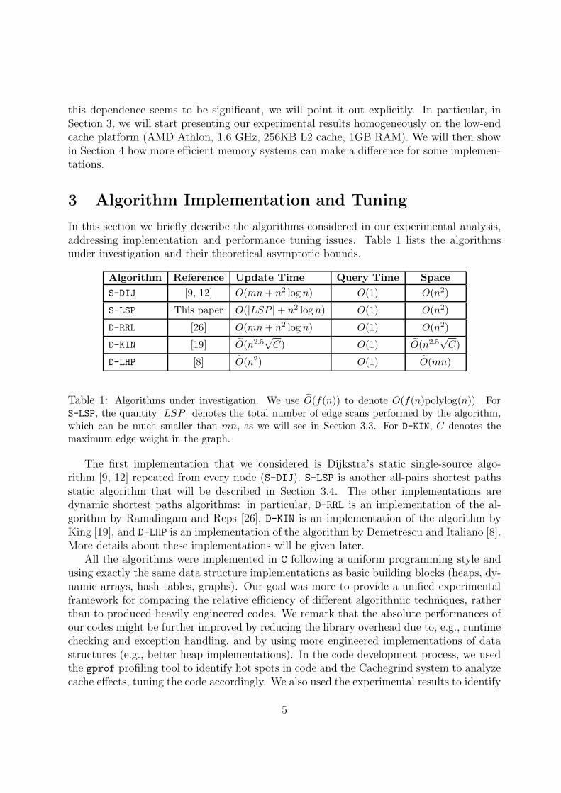
In this section we briefly describe the algorithms considered in our experimental analysis,addressing implementation and performance tuning issues. Table 1 lists the algorithmsunder investigation and their theoretical asymptotic bounds.
Algorithm Reference Update Time Query Time Space
S-DIJ [9, 12] O(mn + n2 log n) O(1) O(n2)
S-LSP This paper O(|LSP | + n2 log n) O(1) O(n2)
D-RRL [26] O(mn + n2 log n) O(1) O(n2)
D-KIN [19] O(n2.5√
C) O(1) O(n2.5√
C)
D-LHP [8] O(n2) O(1) O(mn)
Table 1: Algorithms under investigation. We use O(f(n)) to denote O(f(n)polylog(n)). ForS-LSP, the quantity |LSP | denotes the total number of edge scans performed by the algorithm,which can be much smaller than mn, as we will see in Section 3.3. For D-KIN, C denotes themaximum edge weight in the graph.
The first implementation that we considered is Dijkstra’s static single-source algo-rithm [9, 12] repeated from every node (S-DIJ). S-LSP is another all-pairs shortest pathsstatic algorithm that will be described in Section 3.4. The other implementations aredynamic shortest paths algorithms: in particular, D-RRL is an implementation of the al-gorithm by Ramalingam and Reps [26], D-KIN is an implementation of the algorithm byKing [19], and D-LHP is an implementation of the algorithm by Demetrescu and Italiano [8].More details about these implementations will be given later.
All the algorithms were implemented in C following a uniform programming style andusing exactly the same data structure implementations as basic building blocks (heaps, dy-namic arrays, hash tables, graphs). Our goal was more to provide a unified experimentalframework for comparing the relative efficiency of different algorithmic techniques, ratherthan to produced heavily engineered codes. We remark that the absolute performances ofour codes might be further improved by reducing the library overhead due to, e.g., runtimechecking and exception handling, and by using more engineered implementations of datastructures (e.g., better heap implementations). In the code development process, we usedthe gprof profiling tool to identify hot spots in code and the Cachegrind system to analyzecache effects, tuning the code accordingly. We also used the experimental results to identify
5

a good setting of the relevant parameters of each implementation. The source code of ourimplementations is distributed under the terms of the GNU Lesser General Public Licenseand is available at the URL http://www.dis.uniroma1.it/~demetres/experim/dsp/
along with the full experimental package, including test sets, generators, and scripts toreproduce the experiments described in this paper.
3.1 The Algorithm by Ramalingam and Reps (D-RRL)
The algorithm by Ramalingam and Reps [26] works on a directed graph G with strictlypositive real-valued edge weights and maintains information about the shortest paths froma given node s. In particular, it maintains a directed acyclic subgraph of G containing allthe edges that belong to at least one shortest path from s. To support an edge weightupdate, the algorithm first computes the subset of nodes whose distance from s is affectedby the update. Distances are then updated by running a Dijkstra-like procedure on thosenodes. Maintaining single-source shortest paths from s requires O(ma + na log na) perupdate, where na is the number of nodes affected by the update and ma is the number ofedges having at least one affected endpoint. This yields a O(mn + n2 log n) time bound inthe worst case for dynamic all pairs shortest paths.
Our implementation.
The algorithm by Ramalingam and Reps is known to be very fast in practice (see, e.g., [6,11, 13]). In our implementation, we considered a further simplified version of the originalalgorithm, which was previously described in [6]. This lighter version, which we refer toas D-RRL, maintains a shortest paths tree instead of a directed acyclic subgraph, and doesnot spend time in identifying nodes that do not change distance from the source after anupdate. If the graph has only a few different paths having the same weight (as in thereal-world inputs we considered), this variant can be much faster (see [6]) than the originalalgorithm in [26].
3.2 The Algorithm by King (D-KIN)
The dynamic shortest paths algorithm by King [19] works on directed graphs with smallinteger weights. The main idea behind the algorithm is to maintain dynamically all pairsshortest paths up to a distance d, and to recompute longer shortest paths from scratch ateach update by stitching together shortest paths of length ≤ d.
To maintain shortest paths up to distance d, the algorithm keeps a pair of in/outshortest paths trees IN(v) and OUT (v) of depth ≤ d rooted at each node v. Trees IN(v)and OUT (v) are maintained with a variant of the decremental data structure by Even andShiloach [10]. It is easy to prove that, if the distance dxy between any pair of nodes x andy is at most d, then dxy is equal to the minimum of dxv + dvy over all nodes v such thatx ∈ IN(v) and y ∈ OUT (v). To support updates, insertions/decreases of edges around anode v are handled by rebuilding only IN(v) and OUT (v), while edge deletions/increases
6
Experiment for increasing max weight C (rnd, 500 vertices, 1500 edges)
0
5
10
15
20
25
30
0 10 20 30 40 50 60 70 80 90 100
Maximum edge weight C
Tim
e pe
r up
date
(se
c.)
D-KIN
Experiment for increasing max weight C (rnd, 500 vertices, 1500 edges)
0
50
100
150
200
250
300
350
400
0 10 20 30 40 50 60 70 80 90 100
Maximum edge weight C
Spac
e (M
B)
D-KIN
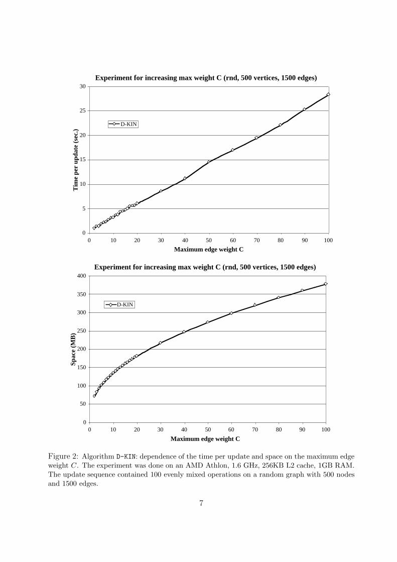
Figure 2: Algorithm D-KIN: dependence of the time per update and space on the maximum edgeweight C. The experiment was done on an AMD Athlon, 1.6 GHz, 256KB L2 cache, 1GB RAM.The update sequence contained 100 evenly mixed operations on a random graph with 500 nodesand 1500 edges.
7

are performed via operations on any trees that contain them. The amortized cost of suchupdates is O(n2d) per operation.
To maintain shortest paths longer than d, the algorithm exploits the following property(see, e.g., [16]): if H is a random subset of Θ((Cn log n)/d) nodes in the graph, then theprobability of finding more than d consecutive nodes in a path, none of which are from H ,is very small. Thus, if we look at nodes in H as “hubs”, then any shortest path from x toy of length ≥ d can be obtained by stitching together shortest subpaths of length ≤ d thatfirst go from x to a node in H , then jump between nodes in H , and eventually reach yfrom a node in H . This can be done by first computing shortest paths only between nodesin H using any static all-pairs shortest paths algorithm, and then by extending them atboth endpoints with shortest paths of length ≤ d to reach all other nodes. This stitchingoperations requires O(n2|H|) = O((Cn3 log n)/d) time.
Choosing d =√
Cn log n yields an O(n2.5√
C log n ) amortized update time. Since Hcan be also computed deterministically, the algorithm can be derandomized. While theoriginal algorithm in [19] requires O(n3) space, in [20] King and Thorup showed how toreduce space to O(n2.5
√C ). The interested reader can find the low-level details of the
algorithm in [19, 20].
Our implementation.
Following the techniques for space reduction [20], we implemented a simpler randomizedversion of the algorithm by King, which we refer to as D-KIN. The code is divided into threemodular building blocks: (i) an increase-only data structure for maintaining single-sourceshortest paths up to distance d; (ii) a forest of in/out trees for maintaining all pairs shortestpaths up to distance d under fully dynamic update sequences; (iii) a data structure thatmaintains a forest of in/out trees and performs stitching to rebuild shortest paths longerthan d.
Since the maximum edge weight C is involved in the theoretical bounds, we conductedsome experiments aimed at evaluating the effect of increasing C on the update time andspace. For instance, the experiment considered in Figure 2 shows that while going from arandom graph with 500 nodes, 1500 edges, and maximum weight C = 10 to a graph withthe same size and C = 100, the running time can degrade by about a factor of 10, andthe space usage can degrade by about a factor of 3. Note that, while the space is growingas predicted by the theoretical analysis, the time bound appears to grow linearly in thegiven range of C: this is most probably due to the O(n2.5
√C log n ) bound not being tight
for small values of C. Since C can be as high as 20, 000 in Internet graphs and as high as200, 000 in US road networks, we could not run D-KIN on these real-world inputs.
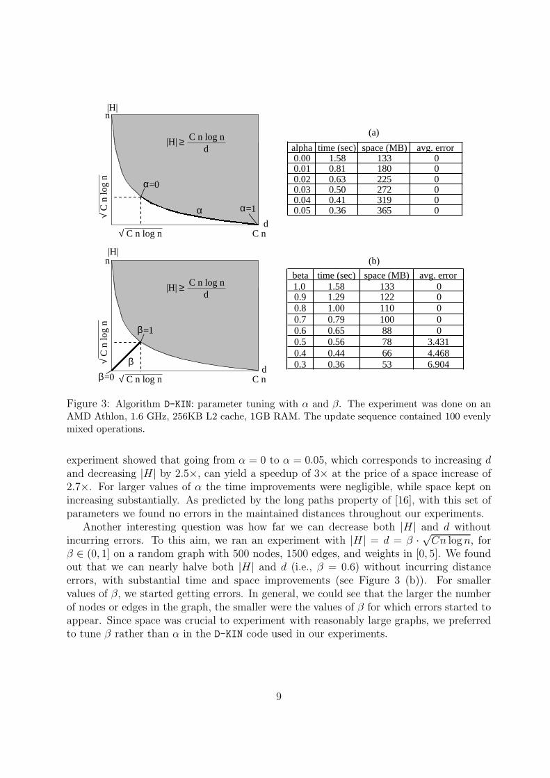
Profiling information revealed that with the standard setting |H| = d =√
C log n,typically more than 75% of the update time is required by the path stitching procedure.We thus expected a reduction of |H| to yield substantial benefits in the running time, andthis was fully confirmed by our experiments. As an example, Figure 3 (a) shows the resultof an experiment on a random graph with 500 nodes, 1500 edges, and weights in [0, 5],where we set |H| = Cn log n
dand d = (1 − α)
√Cn log n + α · Cn, for α ∈ [0, 0.05]. The
8
n
C n
|H|
d√ C n log n
α
α=0
α=1
|H| ≥ C n log nd
√ C
n lo
g n
n
C n
|H|
d√ C n log n
β=1
≥ C n log nd
√ C
n lo
g n
β=0
β
alpha time (sec) space (MB) avg. error0.00 1.58 133 00.01 0.81 180 00.02 0.63 225 00.03 0.50 272 00.04 0.41 319 00.05 0.36 365 0
beta time (sec) space (MB) avg. error1.0 1.58 133 00.9 1.29 122 00.8 1.00 110 00.7 0.79 100 00.6 0.65 88 00.5 0.56 78 3.4310.4 0.44 66 4.4680.3 0.36 53 6.904
|H|
(a)
(b)
Figure 3: Algorithm D-KIN: parameter tuning with α and β. The experiment was done on anAMD Athlon, 1.6 GHz, 256KB L2 cache, 1GB RAM. The update sequence contained 100 evenlymixed operations.
experiment showed that going from α = 0 to α = 0.05, which corresponds to increasing dand decreasing |H| by 2.5×, can yield a speedup of 3× at the price of a space increase of2.7×. For larger values of α the time improvements were negligible, while space kept onincreasing substantially. As predicted by the long paths property of [16], with this set ofparameters we found no errors in the maintained distances throughout our experiments.
Another interesting question was how far we can decrease both |H| and d withoutincurring errors. To this aim, we ran an experiment with |H| = d = β ·
√Cn log n, for
β ∈ (0, 1] on a random graph with 500 nodes, 1500 edges, and weights in [0, 5]. We foundout that we can nearly halve both |H| and d (i.e., β = 0.6) without incurring distanceerrors, with substantial time and space improvements (see Figure 3 (b)). For smallervalues of β, we started getting errors. In general, we could see that the larger the numberof nodes or edges in the graph, the smaller were the values of β for which errors started toappear. Since space was crucial to experiment with reasonably large graphs, we preferredto tune β rather than α in the D-KIN code used in our experiments.
9

3.3 The Algorithm by Demetrescu and Italiano (D-LHP)
The dynamic shortest path algorithm in [8] works on directed graphs with nonnegativereal-valued edge weights and hinges on the notion of locally shortest paths (LSP): we saythat a path π is locally shortest if every proper subpath of π is a shortest path (note thatπ is not necessarily a shortest path). A historical shortest path is a path that has been ashortest path at some point during the sequence of updates, and none of its edges has beenupdated since then. We further say that a path π in a graph is locally historical if everyproper subpath of π is a historical shortest path. The main idea behind the algorithm isto maintain dynamically the set of locally historical paths (LHP), which include locallyshortest paths and shortest paths as special cases. The following theorem from [8] boundsthe number of paths that become locally historical after each update:
Theorem 1 Let G be a graph subject to a sequence of update operations. If at any timethroughout the sequence of updates there are at most z historical shortest paths betweeneach pair of nodes, then the amortized number of paths that become locally historical ateach update is O(zn2).
To keep changes in locally historical paths small, it is then desirable to have as fewhistorical shortest paths as possible throughout the sequence of updates. To do so, thealgorithm transforms on the fly the input update sequence into a slightly longer equiv-alent sequence that generates only a few historical shortest paths. In particular, it usesa simple smoothing strategy that, given any update sequence Σ of length k, produces anoperationally equivalent sequence F (Σ) of length O(k log k) that yields only O(log k) his-torical shortest paths between each pair of nodes in the graph (see [8]). By Theorem 1,this technique implies that only O(n2 log k) paths become locally historical at each updatein the smoothed sequence F (Σ).
To support an edge weight update operation, the algorithm works in two phases. Itfirst removes all maintained paths that contain the updated edge. Then it runs a dynamicmodification of Dijkstra’s algorithm [9] in parallel from all nodes: at each step a shortestpath with minimum weight is extracted from a priority queue and it is combined withexisting historical shortest paths to form new locally historical paths. The update algo-rithm spends O(logn) time for each of the O(zn2) new locally historical paths. Since thesmoothing strategy lets z = O(logn) and increases the length of the sequence of updatesby an additional O(log n) factor, this yields O(n2 log3 n) amortized time per update. Evenwith smoothing, there can be as many as O(mn log n) locally historical paths in a graph:this implies that the space required by the algorithm is O(mn log n) in the worst case. Werefer the interested reader to [8] for the low-level details of the method.
Our implementation.
Our implementation (D-LHP) followed closely the theoretical algorithm in [8], with two maindifferences. First, in our code, after an update we only process node pairs that are affectedby the change. Second, we implemented one additional heuristic: namely, we stopped
10

Experiment for increasing smoothing threshold (Utah road network)
4
4.5
5
5.5
6
6.5
7
7.5
8
8.5
9
0 0.1 0.2 0.3 0.4 0.5 0.6 0.7 0.8 0.9 1
Smoothing threshold
Tim
e pe
r up
date
(m
sec.
)
D-LHP (initially few historical shortest path)
D-LHP (initially many historical shortest paths)
no smoothing full smoothing
Experiment for increasing smoothing threshold (Utah road network)
5
7
9
11
13
15
17
19
21
23
25
0 0.1 0.2 0.3 0.4 0.5 0.6 0.7 0.8 0.9 1
Smoothing threshold
Spac
e (M
B)
D-LHP (initially few historical shortest paths)
D-LHP (initially many historical shortest paths)
no smoothing full smoothing
Figure 4: Algorithm D-LHP: effects of varying the degree of smoothing on the Utah road networkinitialized from the initial graph (few historical shortest paths), or from the empty graph via edgeinsertions (many historical shortest paths). The experiment was done on an AMD Athlon, 1.6GHz, 256KB L2 cache, 1GB RAM. The update sequence contained 1, 000 evenly mixed operations(after the initialization).
11

performing smoothing whenever the ratio between the number of created LHPs and deletedLHPs exceeded a certain smoothing threshold. In particular, when the smoothing thresholdis 0, no smoothing is in place, while a smoothing threshold equal to 1 corresponds to fullsmoothing. We expected that the main objective of smoothing was to ensure the theoreticalworst-case bounds, but we were not fully convinced of its practical significance. To assessthe effects of smoothing, we performed different experiments on D-LHP for different valuesof the smoothing threshold and for two different data structure initialization methods:
1. Initially at most one historical shortest path per node pair: We started a randomupdate sequence from a data structure having at most one (historical) shortest pathper pair. In this scenario, smoothing did not appear to be of any benefit.
2. Initially many historical shortest paths: We built the data structure via edge inser-tions starting from an empty graph, in order to force artificially the data structureto contain at the beginning of the random update sequence a very large numberof historical shortest paths. We remark that only edge insertions or edge weightdecreases can create new historical shortest paths without destroying existing his-torical shortest paths. In this scenario, our experiments showed that the mainpositive effect of smoothing was to reduce the space usage, but this always cameat the price of a running time overhead.
For example, in Figure 4 we report the results of such an experiment on the Utah roadnetwork (269 nodes and 742 edges). These results suggest that a certain degree of smooth-ing can be useful only when there can be a large number of historical shortest paths in thedata structure. This may happen, e.g., if we have long bursts of edge weight decreases oredge insertions. Since even in this case the payoff of smoothing seemed of limited extent,we decided to use in all our further experiments a D-LHP code with smoothing thresholdset to 0 (i.e., no smoothing).
3.4 A New Static Algorithm Based on Locally Shortest Paths(S-LSP)
Another interesting issue to investigate experimentally was related to the number of locallyshortest paths in a graph. In the worst case, we know that they can be as many as O(mn).But how many of them can we have in “typical” instances? Our experiments showed thatin real-world graphs they tend to be very close to n2, i.e., there is typically only one locallyshortest path between any pair of nodes, which is also a shortest path (see upper chart inFigure 5). For random graphs, this number appears to grow very slowly with the graphdensity (see lower chart in Figure 5).
This suggested that locally shortest paths could be exploited also for static all pairsshortest path algorithms. In particular, we investigated how to deploy locally shortest pathsin Dijkstra-like algorithms in order to reduce substantially the number of total edge scans,which is known to be the performance bottleneck for shortest path implementations on
12

Locally shortest paths in US road networks
0.0
0.5
1.0
1.5
2.0
2.5
3.0
3.5
DE NV NH ME AZ ID MT ND CT NM MA NJ LA CO MD NE MS IN AR KS KY MI IA AL MN MO CA NC
US states
average node degree|LSP| per pair of nodes
Locally shortest paths in random graphs (500 nodes)
36
12
24
48
96
2.1 2.8 4.9 6.2
1.71.10
20
40
60
80
100
120
0 5000 10000 15000 20000 25000 30000 35000 40000 45000 50000Number of edges
average node degree|LSP| per pair of nodes
Figure 5: Number of locally shortest paths in random graphs and in US road networks.
13

dense graphs. We designed a static algorithm, which we refer to as S-LSP, that essentiallyruns Dijkstra’s algorithm in parallel from all nodes and scans only edges in locally shortestpaths to reduce the overall work. The running time of S-LSP is O(|LSP |+n2 log n), where|LSP | is the number of locally shortest paths in the graph. This can yield substantialtime savings whenever |LSP | << mn. For instance, in Figure 6 we report the resultsof an experiment comparing S-LSP and Dijkstra’s algorithm (S-DIJ) on random graphswith 500 nodes and increasing edge density: as it can be seen, while on sparse graphs thedata structure overhead in the algorithms is significant, as the graph becomes denser andedge scanning becomes more relevant in the running times of the algorithms, S-LSP canbe substantially faster than S-DIJ.
Experiment for increasing edge density (rnd, 500 nodes)
0
2
4
6
8
10
12
0 5000 10000 15000 20000 25000 30000 35000 40000 45000 50000
Number of edges
Tim
e pe
r up
date
(se
c.)
S-DIJ
S-LSP
S-LSP
S-DIJ
Figure 6: S-LSP versus S-DIJ on a random graph with 500 nodes, increasing densities, and edgeweights in the range [1, 1000]. The experiment was done on an AMD Athlon, 1.6 GHz, 256KBL2 cache, 1GB RAM. The update sequence contained 1, 000 evenly mixed operations.
Note that S-LSP has a similar flavor as the hidden paths algorithm by Karger et al. [18],which runs in O(m∗n + n2 log n) time, where m∗ is the number of edges that participatein shortest paths. We remark that the two approaches are quite different. To see this,consider the bottleneck graph shown in Figure 1 with edge weights equal to 1: for thehidden paths algorithm we get m∗ = m, since every edge is trivially a shortest path, while|LSP | = O(n2). Thus, the hidden paths algorithm runs in O(mn + n2 log n) time, whileS-LSP runs in O(n2 log n) time. By the optimal-substructure property of locally shortestpaths, it is easy to see that |LSP | ≤ m∗n ≤ mn: thus, S-LSP is never slower than thehidden paths algorithm.
14

Experiment for increasing edge density (rnd, 500 nodes)
0.001
0.01
0.1
1
10
0 5000 10000 15000 20000 25000 30000 35000 40000 45000 50000
Number of edges
Tim
e pe
r up
date
(se
c.)
S-DIJS-LSPD-KIND-RRLD-LHP
S-LSP
S-DIJ
D-LHP
D-RRL
D-KIN
Figure 7: Running times of the different algorithms on random graphs with 500 nodes, increasingdensities, and edge weights in the range [1, 1000]. D-KIN was run with β = 0.6, and integer weightsin the smaller range [1, 5]. The experiment was done on an AMD Athlon, 1.6 GHz, 256KB L2cache, 1GB RAM. The update sequence contained 1, 000 evenly mixed operations; the runningtimes are reported on a logarithmic scale.
4 Overall Discussion
Random inputs.
Our experiments with random graphs pointed out that D-LHP and D-RRL are the fastestimplementations: in this scenario they can be faster than static algorithms (S-DIJ andS-LSP) even by two to four orders of magnitude, depending on the inputs. AlgorithmD-KIN was only at most one order of magnitude faster than the static algorithms: thisseems to be mainly due to the high overhead caused by maintaining the forest of in/outtrees and by stitching paths in the data structure. For sparse random graphs, the runningtimes of D-RRL and D-LHP are very close, and the underlying computing platform playsa role in deciding which one performs better (see later for a discussion on this). As thegraph density increases, and consequently the computational savings of locally shortestpaths become more significant (as illustrated also in Figure 5), D-LHP becomes the mostefficient choice on all the platforms we considered. This can be clearly seen in Figure 7,which depicts the result of an experiment on random graphs with 500 nodes, increasingedge densities, and edge weights in the range [1, 1000]. Only the experiment on D-KIN was
15

Experiment for increasing edge density (rnd, 500 nodes)
0
20
40
60
80
100
120
140
160
180
0 5000 10000 15000 20000 25000 30000 35000 40000 45000 50000
Number of edges
Spac
e (M
B)
D-KIN
D-RRL
D-LHP
D-LHP
D-RRL
D-KIN
Figure 8: Space usage of the different dynamic algorithms on random graphs with 500 nodes,increasing densities, and edge weights in the range [1, 1000]. D-KIN was run with β = 0.6, andinteger weights in the smaller range [1, 5].
done with integer weights in the smaller range [1, 5], to avoid the performance degradationof this algorithm for large values of C. Figure 8 reports the space usage of the dynamicimplementations: D-RRL uses simple data structures, retains little information throughoutthe sequence of updates, and thus can save space with respect to D-KIN and D-LHP. Notethat, as correctly predicted by theory, the amount of memory used by D-RRL (O(n2)) and byD-KIN (O(n2.5
√C )) does not depend upon the graph density, while the space requirement
of D-LHP (O(|LHP | + n2)) depends on the number of locally historical paths and thusvaries substantially with the graph and with its density.
Bottleneck inputs.
Bottleneck inputs (see Figure 1) force a pathological sequence of updates, changing theweight of many shortest paths and causing the algorithm to rescan a large portion of thegraph during each update. Figure 9 shows the result of an experiment with bottleneckgraphs of different densities on two different platforms: our low-end cache system (256KBL2 cache) and our high-end cache system (1.4MB L2 cache, 32MB L3 cache). We firstdiscuss some features which appear to be architecture-independent, and then analyze theeffects of the underlying platforms on the implementations.
As it can be seen from Figure 9, D-RRL is hit pretty badly by those inputs, and becomes
16

Experiment on bottleneck graphs (500 nodes, AMD Athlon)
0
0.2
0.4
0.6
0.8
1
1.2
1.4
1.6
1.8
0 5000 10000 15000 20000 25000 30000
Number of edges
Tim
e pe
r up
date
(se
c.)
S-DIJS-LSPD-RRLD-LHP
S-LSP
S-DIJ
D-LHP
D-RRL
(a) Experiment on an AMD Athlon, 1.6 GHz, 256KB L2 cache, 1GB RAM.
Experiment on bottleneck graphs (500 nodes, IBM Power4)
0
0.2
0.4
0.6
0.8
1
1.2
1.4
1.6
1.8
0 5000 10000 15000 20000 25000 30000
Number of edges
Tim
e pe
r up
date
(se
c.)
S-DIJS-LSPD-RRLD-LHP
D-RRL
S-DIJ
D-LHP
S-LSP
(b) Experiment on an IBM Power 4, 1.1 GHz, 1.4MB L2 cache, 32MB L3 cache, 64GB RAM.
Figure 9: Experiment on bottleneck graphs of different sizes. The update sequence contained1, 000 evenly mixed operations.
17

even slower than the static implementation of Dijkstra (S-DIJ). This reflects the fact thatthe worst-case update time of the algorithm by Ramalingam and Reps is asymptoticallythe same as the static algorithm, and thus the performance of D-RRL can be quite badon hard instances. On the other side, in those inputs D-LHP becomes comparable to itsstatic version S-LSP. This can be explained by noting that for those inputs most of thecomputation savings of D-LHP come from locally shortest paths, which are O(n2) in thiscase. Since bottleneck inputs force scanning of a large portion of the graph, D-LHP andS-LSP end up performing similar tasks on those test sets.
In all our experiments with bottleneck inputs, D-LHP was substantially faster than eitherD-RRL or S-DIJ on dense graphs or on platforms with a good cache system. The first casecan be easily explained by considering the computational savings of locally shortest pathson dense graphs. To explain the second case, we consider more closely Figure 9 (a) andFigure 9 (b). In the two experiments, the running times of D-RRL and S-DIJ are verysimilar, while the implementations based on locally shortest paths (D-LHP and S-LSP)have a speedup of more than 2 on the high-end cache system. Since the CPU clocks of thetwo platforms are comparable, this may suggest that algorithms based on locally shortestpaths, which retain more information throughout the updates, seem to benefit more frombetter memory systems. Moreover, we observe that D-RRL and S-DIJ, besides requiringless space than D-LHP, tend to have a more regular pattern of data access, since theyrecompute single-source shortest paths starting repeatedly from every node in the graph,as opposed to D-LHP and S-LSP, which compute all shortest paths in parallel, and thusneed to access more global data structures. Consequently, D-RRL and S-DIJ seem to sufferless from reduced cache sizes. We will investigate more closely this issue next.
Real-world inputs.
The same general trend observed for random graphs can be seen also in our experimentswith real-word graphs: in particular, D-RRL and D-LHP are much faster than the otherimplementations (1–3 orders of magnitude). This is illustrated in Figure 10, which reportsthe results of our experiments on US road networks and AS Internet networks with com-pletely random edge updates. The chart shows the running time of all algorithms exceptfor D-KIN, which was omitted from our experiments on real-world inputs due to its pro-hibitive performance degradation in case of large edge weights. Once again, D-LHP requiresmore space than D-RRL as illustrated in Figure 11.
The results of our experiments on real-world inputs with edge weight updates within5% of their original value are illustrated in Figure 12. In this scenario, there seems to beconsistent performance gain of D-LHP over D-RRL, which can be explained as follows. Whenthe update range becomes smaller, also the portion of the graph affected by the change islikely to be smaller. D-LHP, which is based on locally shortest paths, seems to be able toexploit more effectively the locality of this change. This is confirmed by the reduced spaceusage of D-LHP in this framework, as reported in Figure 13.
Similarly to the experiments on bottleneck inputs, the running times of D-LHP andD-RRL can be very close and their relative performance seems to vary on different platforms.
18

Experiment on US road networks
0.001
0.01
0.1
1
10
100 200 300 400 500 600 700 800 900 1000
Number of nodes
Tim
e pe
r up
date
(se
c.)
S-DIJS-LSPD-RRLD-LHP
S-LSP
S-DIJ
D-LHP
D-RRL
Experiments on AS networks
0.0001
0.001
0.01
0.1
1
10
100
400 600 800 1000 1200 1400 1600 1800 2000
Number of nodes
Tim
e pe
r up
date
(se
c.)
S-DIJS-LSPD-RRLD-LHP
S-LSP
S-DIJ
D-LHP
D-RRL
Figure 10: Running times of the different algorithms on US road networks and AS Internetnetworks under sequences of 1, 000 evenly mixed random updates. D-KIN was not applicablesince edge weights are too large in these graphs. The experiment was done on an AMD Athlon,1.6 GHz, 256KB L2 cache, 1GB RAM.
19

Experiment on US road networks
0
20
40
60
80
100
120
140
160
100 200 300 400 500 600 700 800 900 1000
Number of nodes
Spac
e (M
B)
D-RRL
D-LHP
D-LHP
D-RRL
Experiments on AS networks
0
100
200
300
400
500
600
400 600 800 1000 1200 1400 1600 1800 2000
Number of nodes
Spac
e (M
B)
D-RRL
D-LHP
D-LHP
D-RRL
Figure 11: Space usage of D-LHP and D-RLL on US road networks and AS Internet networksunder sequences of 1, 000 evenly mixed random updates.
20

Experiment on US road networks
0.001
0.01
0.1
1
10
100 200 300 400 500 600 700 800 900 1000
Number of nodes
Tim
e pe
r up
date
(se
c.)
S-DIJS-LSPD-RRLD-LHP
S-LSP
S-DIJ
D-LHP
D-RRL
Experiments on AS networks
0.0001
0.001
0.01
0.1
1
10
100
400 600 800 1000 1200 1400 1600 1800 2000
Number of nodes
Tim
e pe
r up
date
(se
c.)
S-DIJS-LSPD-RRLD-LHP
S-LSP
S-DIJ
D-LHP
D-RRL
Figure 12: Running times of the different algorithms on US road networks and AS Internetnetworks under sequences of 1, 000 evenly mixed random updates within 5% of their originalvalue. D-KIN was not applicable since edge weights are too large in these graphs. The experimentwas done on an AMD Athlon, 1.6 GHz, 256KB L2 cache, 1GB RAM.
21

Experiment on US road networks
0
20
40
60
80
100
120
140
160
100 200 300 400 500 600 700 800 900 1000
Number of nodes
Spac
e (M
B)
D-RRL
D-LHP
D-LHP
D-RRL
Experiments on AS networks
0
100
200
300
400
500
600
400 600 800 1000 1200 1400 1600 1800 2000
Number of nodes
Spac
e (M
B)
D-RRL
D-LHPD-LHP
D-RRL
Figure 13: Space usage of D-LHP and D-RLL on US road networks and AS Internet networksunder sequences of 1, 000 evenly mixed random updates within 5% of their original value.
22

Experiment on US road networks using different platforms
2.8
2
1.4
1
1.4
2
2.8
100 200 300 400 500 600 700 800 900 1000
Number of nodes
D-LHP faster than D-RRL
IBM Power 4 (32MB L3 cache)
Sun UltraSPARC IIi (2MB L2 cache)
AMD Athlon (256KB L2 cache)
D-LHP slower than D-RRL
OH
NC
CAMOMN
ALIA
MIKY
KS
AR
INMS
NEMD
CO
LANJ
MACT
NMND
MT
ID
AZ
MENH
NVDE
D-R
RL
/D-L
HP
D-L
HP
/D-R
RL
Cache miss ratio on the Colorado road network
1.45
1.19
1.00
1.17
1.30
1.41
1.83
1.67
1.59
11.12
1.4
1.08
2
1.4
1
1,4
2
128KB 256KB 512KB 1MB 2MB 4MB 8MB 16MB 32MB
Cache size
Simulated cache miss ratioPerformance ratio on real architecturesAthlon
UltraSparc IIi
Power 4
D-R
RL
/D-L
HP
D-L
HP
/D-R
RL
Figure 14: Studying cache effects. (a) Performance ratio max{D-RRL/D-LHP, D-LHP/D-RRL} onthe US road networks using architectures with different cache sizes. (b) Simulated cache missratio max{D-RRL/D-LHP, D-LHP/D-RRL} on the Colorado road network.
23

To illustrate this, we refer to Figure 14 (a), which plots the running time of D-RRL versusthe running time of D-LHP on the US road networks with completely random edge weightupdates measured on platforms with different cache sizes. There are two main phenomenathat can be seen from this figure: first, the relative performance of D-LHP and D-RRL tendsto change with different cache sizes: i.e., the better the cache system, the faster is D-LHP
over D-RRL. Second, on any given platform, D-RRL is likely to become faster than D-LHP asthe number of nodes increases. We believe that both phenomena are due to cache effects:D-LHP requires more memory and uses more global data structures, while D-RRL requiresless space and exhibits a better locality in the memory access pattern. To investigatemore these aspects, we performed an extensive simulation of cache miss ratios with theCachegrind tool [27], and the simulation results on the Colorado road network are reportedin Figure 14 (b). The time ratio measured on different platforms seems to follow the samegeneral trend as the simulated cache miss ratio, which indeed suggests that the relativeperformance of D-RRL and D-LHP on different machines depends on their different cacheusage. The jump from 1.83 to 11.2 in the simulated cache miss ratio for 32MB could beexplained by observing that, in our experiments on the Colorado road network, D-LHP
requires 30.59MB of main memory; this is close to the simulated cache size, and may causethreshold phenomena.
5 Concluding Remarks
In this paper we have implemented, engineered and evaluated experimentally three dif-ferent dynamic shortest path algorithms: D-RRL [26], D-KIN [19] and D-LHP [8]. In ourexperiments, implementing a dynamic algorithm seemed really worth the effort, as allthe dynamic implementations are typically much faster than recomputing a solution fromscratch with a static algorithm: D-RRL and D-LHP can be up to 10,000 times faster than arepeated application of a static algorithm, while D-KIN can be around 10 times faster thana static algorithm.
The algorithm by Ramalingam and Reps (D-RRL) is basically a variant of Dijkstra’salgorithm, and works only on the portion of the graph that is changing throughout updates.Since it uses simple data structures, it seems very hard to beat in situations where theupdates produce a very small change in the solution. However, its worst-case runningtime is asymptotically the same as Dijkstra’s algorithm, and thus it can be quite bad inpathological worst-case instances. The algorithm of Demetrescu and Italiano (D-LHP) usesmore sophisticated data structures than D-RRL, but it still works only on the portion of thegraph that is modified by the updates. It can be as fast as D-RRL on sparse graphs, and itbecomes substantially faster than D-RRL on dense graphs and on worst-case inputs, wherelocally shortest paths seem to gain better payoffs. The main difference in performance withD-RRL on sparse graphs seems related to memory issues, i.e., to the algorithms’ space usageand pattern access on data: in particular, in our experiments D-LHP ran faster on platformswith a good memory hierarchy system (i.e., cache and/or memory bandwidth), while D-RRLseemed preferable on platforms with small cache and/or small memory bandwidth. Overall,
24

D-LHP revealed to be the most robust implementation on different inputs among the oneswe tested. As a side effect, we derived from D-LHP a new static algorithm, S-LSP, whichcan run faster than Dijkstra’s algorithm on dense graphs, since in practice it reducessubstantially the total number of edges scanned.
One issue that seems to deserve further theoretical and empirical study is memoryusage. To answer queries fast, all the algorithms maintain explicitly the all pairs shortestpaths matrix. This makes them hit very soon a “memory wall” in today’s computingplatforms, thus limiting substantially the maximum problem size that can be solved inpractice. Just to make an example, if an implementation requires around 100 bytes pereach pair of nodes in the graph (for instance the space usage of D-LHP is roughly 80 bytesper locally historical path, plus 24 bytes per pair of nodes) on a memory system with 10GB of RAM we can only solve instances of up to 10,000 nodes without incurring memoryswap problems. These were indeed the larger graphs that we were able to consider in ourcomputational study.
Acknowledgments
We are indebted to the anonymous reviewers for many useful comments. We wish tothank Stefano Emiliozzi for his valuable help in the implementation and experimentalanalysis of some of the algorithms discussed in this paper. We deeply acknowledge thegenerous hospitality of Federico Massaioli and CASPUR (Consorzio interuniversitario perle Applicazioni di Supercalcolo Per Universita e Ricerca), which let us run experiments ontheir IBM Power 4.
References
[1] D. Alberts, G. Cattaneo, and G.F. Italiano. An empirical study of dynamic graphalgorithms. ACM Journal on Experimental Algorithmics, 2(5), 1997.
[2] G. Amato, G. Cattaneo, and G.F. Italiano. Experimental analysis of dynamic mini-mum spanning tree algorithms. In Proc. SODA’97, pages 314–323, 1997.
[3] L. Buriol, M. Resende, and M. Thorup. Speeding up dynamic shortest path algorithms.In AT&T Labs Research Report TD–5RJ8B, September 2003.
[4] Cattaneo, G. and Faruolo, P. and Ferraro-Petrillo, U. and Italiano, G. F. Maintainingdynamic minimum spanning trees: An experimental study. In Proceedings of the 4thWorkshop on Algorithm Engineering and Experiments (ALENEX’02), pages 111-125,2002.
[5] B.V. Cherkassky, A.V. Goldberg, and T. Radzik. Shortest paths algorithms: Theoryand experimental evaluation. Math. Programming, 73:129–174, 1996.
25
[6] C. Demetrescu, D. Frigioni, A. Marchetti-Spaccamela, and U. Nanni. Maintainingshortest paths in digraphs with arbitrary arc weights: An experimental study. InProceedings of the 4th Workshop on Experimental Algorithmics (WAE’00), pages 218–229, 2000.
[7] C. Demetrescu and G.F. Italiano. Fully dynamic all pairs shortest paths with realedge weights. In Proc. FOCS’01, pages 260–267, 2001.
[8] C. Demetrescu and G.F. Italiano. A new approach to dynamic all pairs shortest paths.In Proceedings of STOC’03, pages 159–166, 2003.
[9] E.W. Dijkstra. A note on two problems in connexion with graphs. Numerische Math.,1:269–271, 1959.
[10] S. Even and Y. Shiloach. An on-line edge-deletion problem. Journal of the ACM,28:1–4, 1981.
[11] B. Fortz and M. Thorup. Internet traffic engineering by optimizing OSPF weights. InProceedings INFOCOM’00, pages 519–528, 2000.
[12] M.L. Fredman and R.E. Tarjan. Fibonacci heaps and their use in improved networkoptimization algorithms. Journal of the ACM, 34:596–615, 1987.
[13] D. Frigioni, M. Ioffreda, U. Nanni, and G. Pasqualone. Analysis of dynamic algo-rithms for the single source shortest path problem. ACM Journal of ExperimentalAlgorithmics (JEA), 3, 1998.
[14] D. Frigioni, T. Miller, U. Nanni, G. Pasqualone, G. Schafer, and C.D. Zaroliagis. Anexperimental study of dynamic algorithms for directed graphs. In Proc. ESA’98, pages320–331, 1998.
[15] A.V. Goldberg. Shortest path algorithms: Engineering aspects. In Proc. ISAAC’01,pages 502–513, 2001.
[16] D. H. Greene and D.E. Knuth. Mathematics for the analysis of algorithms. Birkhauser,1982.
[17] R. Iyer, D. R. Karger, H. S. Rahul, and M. Thorup. An Experimental Study of Poly-logarithmic, Fully Dynamic, Connectivity Algorithms. ACM Journal of ExperimentalAlgorithmics (JEA), 6, 2001.
[18] D. Karger, D. Koller, and S.J. Phillips. Finding the hidden path: Time bounds forall-pairs shortest paths. SIAM Journal on Computing, 22(6):1199–1217, 1993.
[19] V. King. Fully dynamic algorithms for maintaining all-pairs shortest paths and tran-sitive closure in digraphs. In Proc. FOCS’99, pages 81–99, 1999.
26

[20] V. King and M. Thorup. A space saving trick for directed dynamic transitive closureand shortest path algorithms. In Proc. COCOON’01, pp. 268–277, 2001.
[21] P. Loubal. A network evaluation procedure. Highway Research Record 205, pages96–109, 1967.
[22] J. Murchland. The effect of increasing or decreasing the length of a single arc onall shortest distances in a graph. Technical report, LBS-TNT-26, London BusinessSchool, Transport Network Theory Unit, 1967.
[23] Paolo Narvaez, Kai-Yeung Siu, and Hong-Yi Tzeng. New dynamic algorithms forshortest path tree computation. IEEE/ACM Transactions on Networking, 8:734–746,2000.
[24] Paolo Narvaez, Kai-Yeung Siu, and Hong-Yi Tzeng. New dynamic SPT algorithmbased on a ball-and-string model. IEEE/ACM Transactions on Networking, 9:706–718, 2001.
[25] G. Ramalingam. Bounded incremental computation. Lecture Notes in ComputerScience 1089, 1996.
[26] G. Ramalingam and T. Reps. An incremental algorithm for a generalization of theshortest path problem. Journal of Algorithms, 21:267–305, 1996.
[27] J. Seward and N. Nethercote. Valgrind, an open-source memory debugger for x86-gnu/linux. URL: http://developer.kde.org/~sewardj/.
[28] M. Thorup. Fully-Dynamic All-Pairs Shortest Paths: Faster and Allowing Nega-tive Cycles. Proceedings of the 9th Scandinavian Workshop on Algorithm Theory(SWAT’04), Humlebæk, Denmark, July 8–10, 2004.
[29] F. Zhan and C. Noon. Shortest path algorithms: An evaluation using real roadnetworks. Transportation Science, 32(1):65–73, 1998.
27