experimental and computational investigation of indoor air quality

(This is a sample cover image for this issue. The actual cover is not yet available at this time.)

This article appeared in a journal published by Elsevier. The attachedcopy is furnished to the author for internal non-commercial researchand education use, including for instruction at the authors institution

and sharing with colleagues.

Other uses, including reproduction and distribution, or selling orlicensing copies, or posting to personal, institutional or third party

websites are prohibited.

In most cases authors are permitted to post their version of thearticle (e.g. in Word or Tex form) to their personal website orinstitutional repository. Authors requiring further information

regarding Elsevier’s archiving and manuscript policies areencouraged to visit:

http://www.elsevier.com/copyright

http://www.elsevier.com/copyright

Author's personal copy

Experimental and computational investigation of indoor air quality inside severalcommunity kitchens in a large campus

Shubhajyoti Saha, Abhijit Guha*, Subhransu RoyMechanical Engineering Department, Indian Institute of Technology, Kharagpur, Pin 721302, India

a r t i c l e i n f o

Article history:Received 1 June 2011Received in revised form12 September 2011Accepted 19 October 2011

Keywords:Indoor air qualityComputational fluid dynamics3-dimensional CFDTemperatureFluid flow fieldObnoxious gases

a b s t r a c t

The present work deals with the experimental and computational investigation of the air quality inselected kitchens in the campus of a large institute in India. Four kitchens have been carefully selectedafter a detailed initial survey of the cooking arrangement and exhaust systems in all of the kitchens in thecampus. For the experimental part, the concentrations of CO2 and CO and temperature are recorded withthe help of an indoor air quality measurement device named IAQ Calc7545. In each of the four kitchens,a 1.8 m � 1.5 m vertical area was selected, which is perpendicular to the vertical side of a burner thatfaces the cooks, and measurements were carried out at 72 suitable grid points within this area. For thecomputational part, the three-dimensional fluid flow field in the kitchen of site 1 is numerically simu-lated by Fluent. The volume fractions of CO2 and CO at the outlet of the burners are estimated froma separate FORTRAN code for equilibrium chemical analysis and are used as a boundary condition for theFluent simulation. The mixture model for the multiphase flow in Fluent is used for finding the distri-bution of the species within the flow domain. Given the complexity of the geometry and flow fieldconsidered here, the results of CFD modelling agree well with the experiments, validating the choice ofboundary conditions, grid generation and other subtleties involved. The measured and computed valuesare compared with the corresponding ASHRAE standard.

� 2011 Elsevier Ltd. All rights reserved.

1. Introduction

Indoor air quality (IAQ) has been receiving more and moreattention and increasing interest has been directed towardscontrolling of indoor obnoxious gases such as CO2, CO etc. Ina hostel’s kitchen, working conditions are especially demanding.The air quality is affected by high emission rate of contaminantsreleased from the cooking processes. Ventilation plays an impor-tant role in providing comfortable and productive working condi-tions and in securing contaminant removal. There are three mainfactors affecting thermal comfort, these being: air temperature, airvelocity and air humidity.

In the present work, a detailed analysis is performed to studythe distribution of obnoxious gases and temperature. One difficultywhen attempting to predict the detailed indoor air flow is thatthere are many factors which influence or govern the flow. It isaffected by the details of the air distribution design, buildingconstruction, outdoor environment, and the presence and activitiesof the human beings occupying the space, among many other

factors. When designing and analyzing heating, ventilation and air-conditioning (HVAC) systems, engineers and scientists generallyhave at their disposal three tools to study the indoor air flowpatterns: analytical model, full scale or small scale modelmeasurements and computational fluid dynamics (CFD). Analyticalmodels are usually restricted by the need for simplifying assump-tions and simplistic configurations. Full scale measurements canprovide the most reliable data, but are most expensive and difficult(or mostly impossible) to perform. Extrapolation from small scalemodel data to a real size room or building is limited by scalingdifficulties. CFD seems to be a general and accessible method, butthis too faces several challenges. For the application of CFD toindoor air flow, the challenges include modelling the physics of theflow including turbulence, specifying realistic boundary conditions,representing the complex geometry of the room and developingaccurate and efficient numerical algorithms.

The published studies demonstrate quite clearly the health riskof the cooking. Thiebaud et al. [1] indicates that the fumes gener-ated by frying pork and brief are mutagenic. Hence the chefs areexposed to relatively high levels obnoxious gases such as CO2, CO,air bone mutagens and carcinogens. Vainiotalo [2] carried outmeasurements at eight work places. The survey confirmed thatcooking fumes contain hazardous components. It also indicated

* Corresponding author. Tel.: þ91 3222 281768; fax: þ91 3222 282278.E-mail address: [email protected] (A. Guha).

Contents lists available at SciVerse ScienceDirect

Building and Environment

journal homepage: www.elsevier .com/locate/bui ldenv

0360-1323/$ e see front matter � 2011 Elsevier Ltd. All rights reserved.doi:10.1016/j.buildenv.2011.10.015

Building and Environment 52 (2012) 177e190


that the kitchen worker may be exposed to relatively highconcentrations of pollutants. The quality of indoor air is alsoaffected by the formation, transport, and deposition [3,4] ofparticulate material, which have not been included in the presentwork.

Although cigarette smoking is considered to be the mostimportant case of lung cancer [5], smoking behaviour cannot fullyexplain the epidemiological characteristic of lung cancer amongasian women who rarely smoke but contract lung cancer relativelyoften. A study by Ng [5] found that over 97% of the women inSingapore do not smoke. Thus the presumable source of indoor airpollution for housewives is passive smoking and cooking. Theaforementioned study indicated that greater relative odds ofrespiratory symptoms were associated with increasing weeklyfrequency of gas cooking.

The above studies establish the importance of an well-designedventilation system in kitchens. The efficacy of the exhaust systemshould be especially emphasized. It can be shown that the captureefficiency of the hood equals the ratio of the capture flow rate to thetotal plume flow rate at the front of canopy height [6]. The totalsystem must be designed such that the impurities are effectivelyremoved and do not spread throughout the kitchen. The totalisticapproach of ventilation design should be used to fulfil all needs ofindoor air conditions. This means that the ventilation system isdesigned based on target values of indoor air quality (IAQ), and theactual total heat loads and emission characteristics of the kitchenappliances.

Modelling plays a key role in indoor environmental design.Computational fluid dynamics (CFD) is used for simulating air flowphenomena. CFD methods are based on the solution of the dis-cretized form of the NaviereStokes equations on a grid of pointscombined with turbulence modelling. A computational investiga-tion [7] in a simple geometry shows the effects of main physicalfactors like inlet, exhaust location, air flow rate on the distributionof contaminant concentration in a workroom. The amount ofventilation in an indoor environment under various inlet and outletarrangements has also been investigated [8] using both numericalanalysis and experimental validation. Although CFD can result inmore accurate predictions (as compared to analytical, semi-empirical or small scale studies) when modelling indoor spacesor localized phenomena such as drafts and acute pollutant expo-sures, i.e. in situations where the well-mixed assumption does nothold, special care has to be taken in defining the computationalgrid, in setting boundary conditions and in assigning the physicalproperties of the models [9]. The CFD approach is also limited by itsrequirements on computational costs.

The prediction from a CFD simulation regarding the accumula-tion of air contaminants shows how the accumulation is related tothe location of gas fire in a conventional kitchen [10]. CFD can alsobe used for parametric modelling of domestic kitchen hood topermit the rapid modification of fundamental parameters, such asthe number of blades and the twist angle of the fan [11]. This is animportant point which concerns architects, designers and in somecases healthcare professionals [12]. CFD analysis predicts velocity,temperature and concentration values throughout the solutiondomain, and an analysis of these parameters makes it possible toinfer modifications to the fluid flow patterns or boundary condi-tions (exhaust fans, vents). The flexibility of this methodologyprovides insights into engineering and architectural design alter-natives for improving the indoor air environment in the kitchen.

The objective of the present work is to study, experimentallyand computationally, the indoor air quality of several kitchens inthe campus of a large institute in India. Four kitchens (referred tohere as site 1, site 2 etc.) have been carefully selected aftera detailed initial survey of all large kitchens in the campus. Sites 1, 2,

3 and 4 serve 3/4meals/snacks for approximately 320, 300, 500 and600 people at each meal respectively per day. The measured andcomputed values are to be compared with each other and with thecorresponding ASHRAE standard [13].

2. Experimental method and results

Themain objective of this work is to carry out air quality surveysin different hostel’s and canteen’s kitchens. The readings are takenwithout disturbing the normal working routine of the kitchen sothat the measured values represent the actual working conditions.At each location, experimental measurements took about twohours per data set.

2.1. Site selection

In this experimental work, four kitchens are selected based ontheir type, namely: 1. a large kitchenwith exhaust fans, 2. a kitchenwith general or dilution ventilation system, 3. a small hot andhumid kitchen, 4. a modern kitchen with local exhaust ventilation(LEV) system.

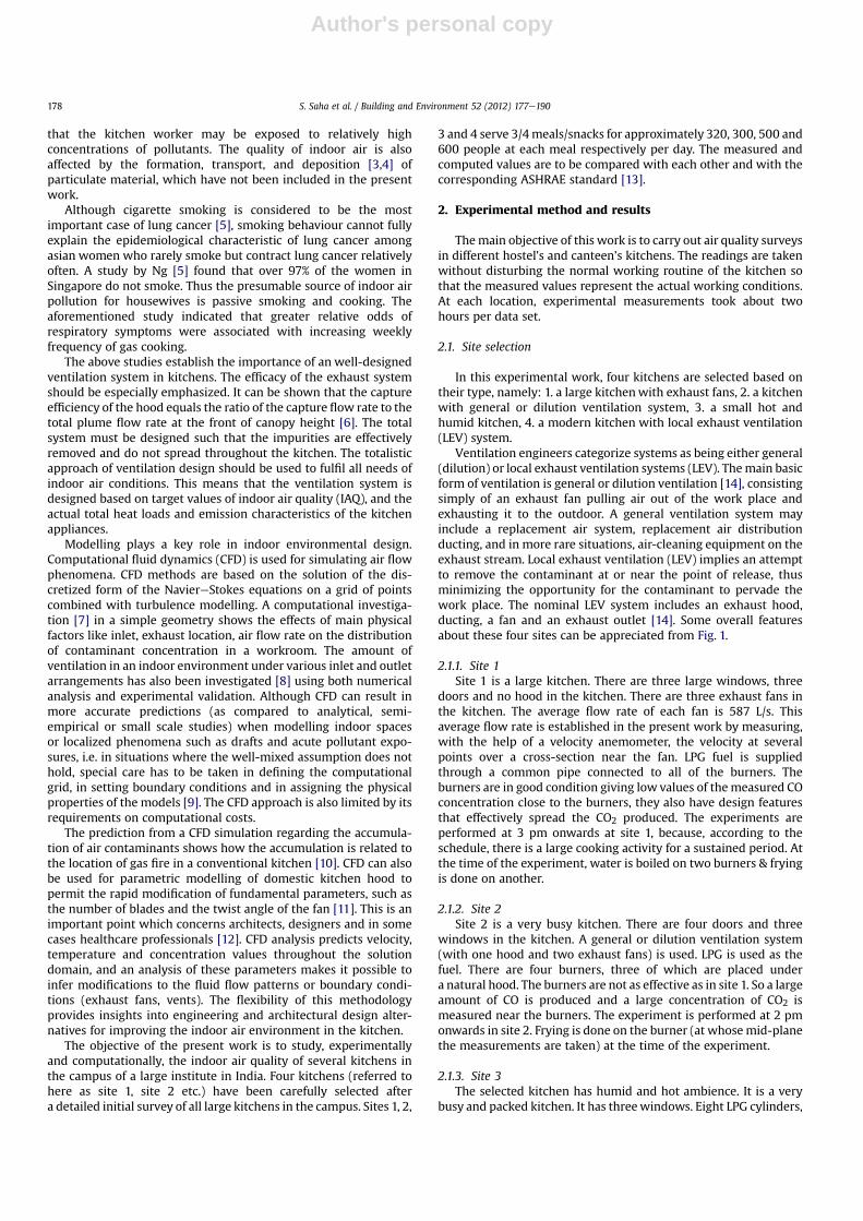
Ventilation engineers categorize systems as being either general(dilution) or local exhaust ventilation systems (LEV). Themain basicform of ventilation is general or dilution ventilation [14], consistingsimply of an exhaust fan pulling air out of the work place andexhausting it to the outdoor. A general ventilation system mayinclude a replacement air system, replacement air distributionducting, and in more rare situations, air-cleaning equipment on theexhaust stream. Local exhaust ventilation (LEV) implies an attemptto remove the contaminant at or near the point of release, thusminimizing the opportunity for the contaminant to pervade thework place. The nominal LEV system includes an exhaust hood,ducting, a fan and an exhaust outlet [14]. Some overall featuresabout these four sites can be appreciated from Fig. 1.

2.1.1. Site 1Site 1 is a large kitchen. There are three large windows, three

doors and no hood in the kitchen. There are three exhaust fans inthe kitchen. The average flow rate of each fan is 587 L/s. Thisaverage flow rate is established in the present work by measuring,with the help of a velocity anemometer, the velocity at severalpoints over a cross-section near the fan. LPG fuel is suppliedthrough a common pipe connected to all of the burners. Theburners are in good condition giving low values of themeasured COconcentration close to the burners, they also have design featuresthat effectively spread the CO2 produced. The experiments areperformed at 3 pm onwards at site 1, because, according to theschedule, there is a large cooking activity for a sustained period. Atthe time of the experiment, water is boiled on two burners & fryingis done on another.

2.1.2. Site 2Site 2 is a very busy kitchen. There are four doors and three

windows in the kitchen. A general or dilution ventilation system(with one hood and two exhaust fans) is used. LPG is used as thefuel. There are four burners, three of which are placed undera natural hood. The burners are not as effective as in site 1. So a largeamount of CO is produced and a large concentration of CO2 ismeasured near the burners. The experiment is performed at 2 pmonwards in site 2. Frying is done on the burner (at whosemid-planethe measurements are taken) at the time of the experiment.

2.1.3. Site 3The selected kitchen has humid and hot ambience. It is a very

busy and packed kitchen. It has threewindows. Eight LPG cylinders,

S. Saha et al. / Building and Environment 52 (2012) 177e190178


each containing 14.2 kg of the cooking gas, are required for thepurpose of cooking in the kitchen in a week. The environment isvery hazardous around 8 am, when all the four burners are usedsimultaneously. The measurements reported in this study aretherefore performed between 8 and 9 am. There are three windows(exposed to the open atmosphere) and two doors (which open intothe dining hall) playing the important role for ventilation. There isno external hood over the burners. Pollutants are expelled by twoexhaust fans from the kitchen, located at the top of one wall of theroom.

2.1.4. Site 4It is the most modern out of the four selected kitchens. It has

a local exhaust ventilation (LEV) system for each burner, which isvery effective to expel different obnoxious gases and hot air whichare formed due to cooking processes. So the measured pollutantconcentration is found to be very near to the acceptable range at thebreathing zone plane though the measured temperature is wellabove the ASHRAE standard. It is a moderate size kitchen. There arefour doors in the kitchen, which provide some ventilation, but thereis no window at all. There are six burners, three of which areworking at the time of the experiment. All burners are LPG based.Ten LPG cylinders are consumed in three days in the discussedkitchen. Three to four persons are engaged in the kitchen forcooking purpose. The working load of the kitchen is not very high.

The experiment is done at 9.00 am onwards. At the time of theexperiment, potatoes and fishes are fried. The flow rate through theburner is set at its maximum. There are three exhaust fans in thekitchen. The average flow rate through an exhaust fan is measuredas 2550 L/s: as compared to the other kitchens, the fans are larger insize and are in relatively better condition. The outlets of theventilator and exhaust fans are accessible in this site and hence anadditional set of measured data for the pollutant concentration isrecorded in this case. The measured concentrations of CO2 near theventilator and exhaust fans are 1376 ppm and 1123 ppm respec-tively. So the ventilator and exhaust fans play a major role to expeldifferent obnoxious gases from the discussed kitchen. Site 4 can beconsidered as the nearest to an ideal kitchen by comparingdifferent measured parameters with the ASHRAE standard.

2.2. Methods of measurement

For the experimental part of the present work, the concentra-tion of CO2, CO and temperature are recorded with the help of anindoor air quality measurement device - IAQ Calc7545 [15]. In eachof the four kitchens, a 1.8 m � 1.4 m vertical area was selected,which is perpendicular to the vertical side of a burner that faces thecooks, and measurements were carried out at 72 suitable gridpoints within this area. The selected area is at the mid-plane ofa burner, has a vertical extent of 1.8 m, and extends in the

Fig. 1. Picture of the four selected sites showing some overall features and internal arrangements.

S. Saha et al. / Building and Environment 52 (2012) 177e190 179


horizontal direction such that the two sides lie respectively at 0.1 mand 1.5 m away from the burner. Measurements are also done infront of the burners on another vertical plane which is perpen-dicular to the previous measuring plane and is at 0.1 m away fromthe burner. A 1.8 m � 1.4 m area was selected, over which themeasurements were carried out. The measurements were taken at72 suitable grid points within this area.

Readings are takenwith the help of IAQ Calc7545 in the constantkeymodewith a sampling interval of 5 s. The outside air conditionshave also been recorded and are used as a basis of comparison forthe conditions inside the kitchen. The Log Dat 2M software [15] isused to export the stored data in the memory of the IAQ Calcrecorder to an Excel spreadsheet for further processing. A velocityanemometer is used to measure velocities at various points ona cross-sectional plane in the vicinity of the exhaust fans; thesedata are used to determine the average flow rate through the fan.

2.3. Experimental results and discussion

The measured values of the concentration of CO2 and CO, and oftemperature are plotted in Figs. 2, 3 and 4 as a function of thedistance from the gas burner. In order to avoid cluttering, for eachof the three measured variables, values are shown here only at twodifferent heights above the ground: of these, the height of 0.6 mindicates the position of the burner top and the height of 1.6 m isrepresentative of the nose level or the typical breathing zone plane.The ASHRAE standards for different parameters of indoor air qualityare given in Table 1, so that the measured data can be assessed inthe proper context. The concentration level of different obnoxiousgases and temperature of the four sites are discussed in thefollowing sub-sections.

Now the concentration level of different obnoxious gases andtemperature of four sites are considered separately.

2.3.1. Carbon-dioxideCarbon-dioxide is a normal constituent of exhaled breath. The

outdoor level of carbon-dioxide is usually 350e450 parts permillion (ppm). The carbon-dioxide level is usually greater insidea building than outside. If the indoor carbon-dioxide level is morethan 1000 ppm, when there is inadequate ventilation, there may behealth implications and the occurrence of physical conditions suchas headache, fatigue, and irritation of the eyes and the throat[16,17].

The measured values of CO2 are shown in Fig. 2. The ASHRAEstandard of CO2 is also shown by a black bar in Fig. 2. Themaximumconcentration at nose level of site 1 is 462 ppm. It is observed ata distance 0.3m away from the burner. So the level of concentrationof CO2 is well below the ASHRAE standard at site 1.

Site 2 is a kitchenwith a natural exhaust hood. From the Fig. 2, itis seen that the concentration of CO2 at nose level of site 2 decreasesas one moves away from the burner. The maximum concentrationof CO2 is 1598 ppm at nose level at 0.1 m away from the burner. Thelevel of CO2 concentration is well above the ASHRAE standard up toa distance 0.2 m from the burner at nose level.

Site 3 is a kitchenwhich is small in size but serves food to a largenumber of customers. The pollutant and humid air are notexhausted to atmosphere due to the non-efficient architecturaldesign. The level of CO2 concentration in site 3 is well above theASHRAE standard up to a distance 0.5 m away from the burner atnose level. The maximum concentration of CO2 is 1710 ppm whichis observed at a distance 0.3m from the burner, which is the highestamong the four kitchens studied. However, the measured

250

500

750

1000

1250

1500

1750

0.1 0.3 0.5 0.7 0.9 1.1 1.3 1.5

Distance away from the burner (meter)

Con

cent

ratio

n of

CO

2 (p

pm)

. ASHRAE Standard

Fig. 2. Comparison ofmeasured concentration of CO2 at different heights as a function ofthe distance in various kitchens. Keys: experimental data of site 1 at height 1.6 m,

experimental data of site 2 at height 1.6 m, experimental data of site 3 atheight 1.6m, experimental data of site 4 at height 1.6m, experimental data ofsite 1 at height 0.6 m, experimental data of site 2 at height 0.6 m, exper-imental data of site 3 at height 0.6 m, experimental data of site 4 at height 0.6 m.

0

9

18

27

36

45

54

63

72

81

90

99

108

0.1 0.3 0.5 0.7 0.9 1.1 1.3 1.5


Con

cent

ratio

n of

CO

(pp

m)

.

ASHRAE Standard

Fig. 3. Comparison ofmeasured concentration of CO at different heights as a function ofthe distance in various kitchens. Keys: experimental data of site 1 at height 1.6 m,

experimental data of site 2 at height 1.6 m, experimental data of site 3 atheight 1.6m, experimental data of site 4 at height 1.6m, experimental data ofsite 1 at height 0.6 m, experimental data of site 2 at height 0.6 m, exper-imental data of site 3 at height 0.6 m. experimental data of site 4 at height 0.6 m.

22

26

30

34

38

42

46

50

0.1 0.3 0.5 0.7 0.9 1.1 1.3 1.5


Tem

pera

ture

(D

egre

e C

elsi

us)

Fig. 4. Comparison ofmeasured temperature (�C) at different heights as a function of thedistance invarious kitchens. Keys: experimental data of site 1 at height 1.6m,experimental data of site 2 at height 1.6 m, experimental data of site 3 at height1.6 m, experimental data of site 4 at height 1.6 m, experimental data of site 1at height 0.6 m, experimental data of site 2 at height 0.6 m, experimentaldata of site 3 at height 0.6 m experimental data of site 4 at height 0.6 m.



concentrations are well below the ASHRAE standard at the burnerheight. The above observations are found due to the convectionphenomena as the hot obnoxious gases rise because of the buoy-ancy force. There are two exhaust fans in the kitchen. But they areunable to maintain healthy indoor air quality in the kitchen.

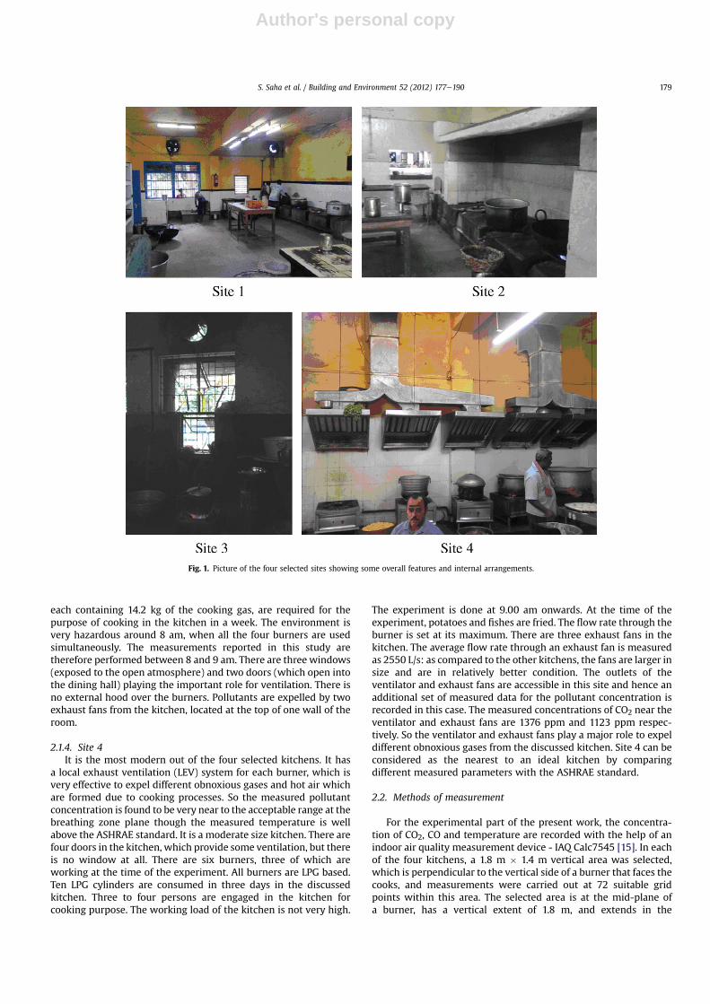
The maximum concentration of CO2 at site 4 at nose level is676 ppm. Fig. 2 shows that the concentration level of CO2, both insite 1 and site 4, is well below the ASHRAE standard up to the noselevel; however, the concentration is higher in site 4. In order tounderstand the interplay of the flow field and concentrationdistribution, the contour plot of CO2 concentration in site 4 is shownin Fig. 5. The effect of the suction through the artificial hood exhaustsystem is clearly visible in Fig. 5. It has been described in Section 2.1that there is very limited natural ventilation in site 4. Therefore, thecombustion products are expelled from the site only through thehoodexhaust system. This iswhy Fig. 5 shows that the concentrationexceeds the ASHRAE standard near the hood inlet in site 4. For thesame reason, a higher concentration of combustion products ispresent in site 4 as compared to site 1, and this trendpersists evenupto a large distance away from the burner, as shown in Fig. 2.

2.3.2. Carbon-monoxideCarbon-monoxide is colourless and odourless, and is a normal

constituent of exhaust gases from incomplete combustion. CO isdangerous (more so than CO2) because it inhibits the blood’s abilityto carry oxygen to vital organs such as the heart and brain. For officeareas, levels of carbon-monoxide are normally between 0 and5 ppm [17]. Concentrations greater than 5 ppm indicates thepossible presence of exhaust gases in the indoor environment andshould be investigated. According to the ASHRAE standard, levels ofcarbon-monoxide inside buildings should not exceed 9 ppm(Table 1). An exposure to a CO level of 35 ppm may cause mildfatigue [17]. If the CO level inside a building is detected above100 ppm, the building should be evacuated until the source isidentified and the situation is corrected [17]. Adverse health effectssuch as headache and dizziness may occur after 2 h exposure to

carbon-monoxide concentrations of 100 ppm [17]. The abovementioned value for 8 h per day, five days per week.

The concentration of carbon-monoxide is high compared to theASHRAE standard in all of the selected sites, as shown in Fig. 3. Site1 is a spacious kitchen but it is not an ideal kitchen with respect tocarbon-monoxide. The maximum concentration of CO is 23.5 ppmat a distance 0.1 m away from the burner which is shown in Fig. 3.The concentration of CO decreases as one moves away from theburner. The average concentration of CO at nose level is above10.4 ppm up to a distance 0.9 m away from the burner. So nose levelconcentration of CO is well above the ASHRAE standard.

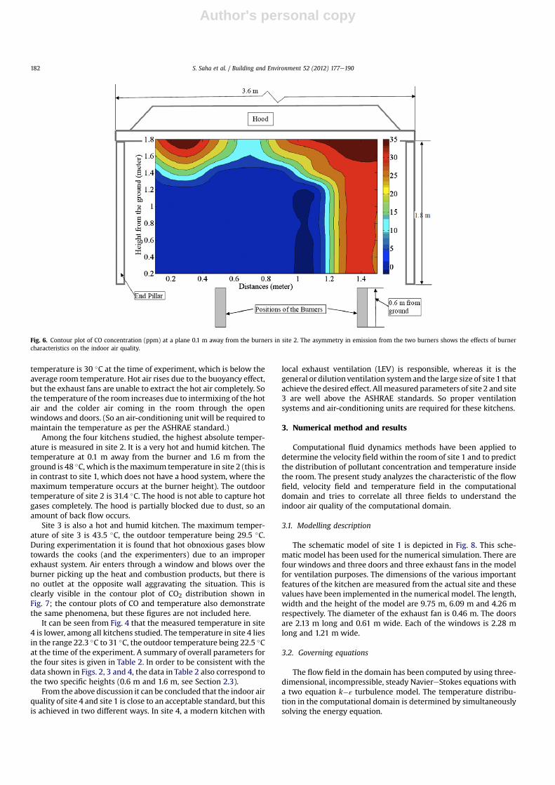
The maximum nose level concentration of CO in site 2 is25.8 ppm at a distance 0.1 m away from the burner. The concen-tration of CO in site 2 is above ASHRAE standard up to a distance0.7 m away from the burner. Fig. 6 depicts another interestingfeature of site 2. The second burner from the left emitsmore amountof CO than the first one; this results in the observed asymmetry inpollutant concentration. So the operating condition of the burners isalso an important factor in determining the indoor air quality.

Among the four kitchens studied, site 3 has the highestconcentration of carbon-monoxide. The concentration of CO atnose level is well above 30 ppm at the farthest point from theburner, which is more than three times of the ASHRAE standard.The maximum concentration at nose level is 102.1 ppm ata distance 0.3 m away from the burner. All these features can beobserved in Fig. 3.

In contrast to site 3, site 4 registers the lowest concentrationlevel of CO at nose level among the four kitchens studied. Themaximum measured value at nose level is 11.4 ppm. So themaximum concentration of CO at nose level is very near to theASHRAE standard and the concentration is below the standard atmost locations at nose level. This phenomenon is observed due topresence of artificial hood exhaust and well-conditioned burners.

2.3.3. TemperatureThe measured distribution of temperature inside the four

kitchens is shown in Fig. 4. The ASHRAE guideline is that indoortemperatures in the winter are maintained between 20 �C to 24 �C.Temperature in the summer should be maintained between 22.8 �Cto 26.1 �C. Continuous exposure at high temperature may causeskin infections [17].

Measurements indicate that the temperature lies in the range of30.5 �C to 35.4 �C in the site 1, as shown in Fig. 4. The maximumtemperature is observed at the burner height. The outdoor

Table 1ASHRAE standard of different parameters.

S.L. no Parameter ASHRAE standard

1 Carbon-dioxide 1000 ppm2 Carbon-monoxide 9 ppm3 Temperature 20 �C to 26.1 �C

Fig. 5. Contour plot of CO2 concentration (ppm) away from the burner in site 4.



temperature is 30 �C at the time of experiment, which is below theaverage room temperature. Hot air rises due to the buoyancy effect,but the exhaust fans are unable to extract the hot air completely. Sothe temperature of the room increases due to intermixing of the hotair and the colder air coming in the room through the openwindows and doors. (So an air-conditioning unit will be required tomaintain the temperature as per the ASHRAE standard.)

Among the four kitchens studied, the highest absolute temper-ature is measured in site 2. It is a very hot and humid kitchen. Thetemperature at 0.1 m away from the burner and 1.6 m from theground is 48 �C, which is themaximum temperature in site 2 (this isin contrast to site 1, which does not have a hood system, where themaximum temperature occurs at the burner height). The outdoortemperature of site 2 is 31.4 �C. The hood is not able to capture hotgases completely. The hood is partially blocked due to dust, so anamount of back flow occurs.

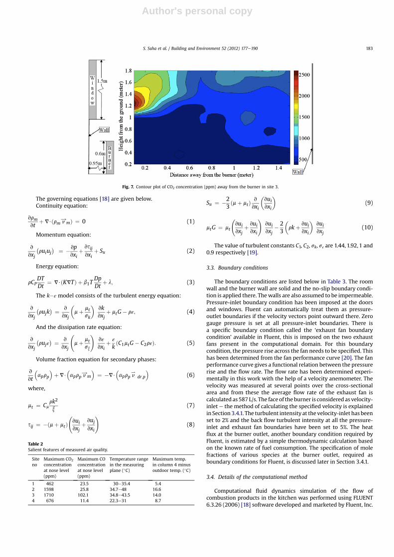
Site 3 is also a hot and humid kitchen. The maximum temper-ature of site 3 is 43.5 �C, the outdoor temperature being 29.5 �C.During experimentation it is found that hot obnoxious gases blowtowards the cooks (and the experimenters) due to an improperexhaust system. Air enters through a window and blows over theburner picking up the heat and combustion products, but there isno outlet at the opposite wall aggravating the situation. This isclearly visible in the contour plot of CO2 distribution shown inFig. 7; the contour plots of CO and temperature also demonstratethe same phenomena, but these figures are not included here.

It can be seen from Fig. 4 that the measured temperature in site4 is lower, among all kitchens studied. The temperature in site 4 liesin the range 22.3 �C to 31 �C, the outdoor temperature being 22.5 �Cat the time of the experiment. A summary of overall parameters forthe four sites is given in Table 2. In order to be consistent with thedata shown in Figs. 2, 3 and 4, the data in Table 2 also correspond tothe two specific heights (0.6 m and 1.6 m, see Section 2.3).

From the above discussion it can be concluded that the indoor airquality of site 4 and site 1 is close to an acceptable standard, but thisis achieved in two different ways. In site 4, a modern kitchen with

local exhaust ventilation (LEV) is responsible, whereas it is thegeneral or dilution ventilation systemand the large size of site 1 thatachieve the desired effect. Allmeasured parameters of site 2 and site3 are well above the ASHRAE standards. So proper ventilationsystems and air-conditioning units are required for these kitchens.

3. Numerical method and results

Computational fluid dynamics methods have been applied todetermine the velocity field within the room of site 1 and to predictthe distribution of pollutant concentration and temperature insidethe room. The present study analyzes the characteristic of the flowfield, velocity field and temperature field in the computationaldomain and tries to correlate all three fields to understand theindoor air quality of the computational domain.

3.1. Modelling description

The schematic model of site 1 is depicted in Fig. 8. This sche-matic model has been used for the numerical simulation. There arefour windows and three doors and three exhaust fans in the modelfor ventilation purposes. The dimensions of the various importantfeatures of the kitchen are measured from the actual site and thesevalues have been implemented in the numerical model. The length,width and the height of the model are 9.75 m, 6.09 m and 4.26 mrespectively. The diameter of the exhaust fan is 0.46 m. The doorsare 2.13 m long and 0.61 m wide. Each of the windows is 2.28 mlong and 1.21 m wide.

3.2. Governing equations

The flow field in the domain has been computed by using three-dimensional, incompressible, steady NaviereStokes equations witha two equation k�ε turbulence model. The temperature distribu-tion in the computational domain is determined by simultaneouslysolving the energy equation.

Fig. 6. Contour plot of CO concentration (ppm) at a plane 0.1 m away from the burners in site 2. The asymmetry in emission from the two burners shows the effects of burnercharacteristics on the indoor air quality.



The governing equations [18] are given below.Continuity equation:

vrmvt

þ V$ðrm v!mÞ ¼ 0 (1)

Momentum equation:

v

vxj

�ruiuj

� ¼ �vpvxi

þ vsijvxi

þ Su (2)

Energy equation:

rCPDTDt

¼ V$ðKVTÞ þ b1TDpDt

þ l; (3)

The k�ε model consists of the turbulent energy equation:

v

vxj

�rujk

� ¼ v

vxj

�mþ mt

sk

�vkvxj

þ mtG� rε; (4)

And the dissipation rate equation:

v

vxj

�rujε

� ¼ v

vxj

mþ mt

sx

!vε

vxiþ ε

kðC1mtG� C2rεÞ: (5)

Volume fraction equation for secondary phases:

v

vt

�aprp

�þ V$

�aprp v!m

�¼ �V$

�aprp v

.dr;p

�(6)

where,

mt ¼ Cmrk2

x(7)

sij ¼ �ðmþ mtÞ vuivxj

þ vujvxi

!(8)

Su ¼ �23ðmþ mtÞ

v

vxi

�vuivxi

�(9)

mtG ¼ mt

vuivxj

þ vuivxi

!vuivxj

� 23

�rkþ vui

vxi

�vuivxj

(10)

The value of turbulent constants C1, C2, sk, sε are 1.44, 1.92, 1 and0.9 respectively [19].

3.3. Boundary conditions

The boundary conditions are listed below in Table 3. The roomwall and the burner wall are solid and the no-slip boundary condi-tion is applied there. Thewalls are also assumed to be impermeable.Pressure-inlet boundary condition has been imposed at the doorsand windows. Fluent can automatically treat them as pressure-outlet boundaries if the velocity vectors point outward there. Zerogauge pressure is set at all pressure-inlet boundaries. There isa specific boundary condition called the ‘exhaust fan boundarycondition’ available in Fluent, this is imposed on the two exhaustfans present in the computational domain. For this boundarycondition, the pressure rise across the fan needs to be specified. Thishas been determined from the fan performance curve [20]. The fanperformance curve gives a functional relation between the pressurerise and the flow rate. The flow rate has been determined experi-mentally in this work with the help of a velocity anemometer. Thevelocity was measured at several points over the cross-sectionalarea and from these the average flow rate of the exhaust fan iscalculated as 587 L/s. The face of theburner is considered as velocity-inlet e the method of calculating the specified velocity is explainedin Section 3.4.1. The turbulent intensity at the velocity-inlet has beenset to 2% and the back flow turbulent intensity at all the pressure-inlet and exhaust fan boundaries have been set to 5%. The heatflux at the burner outlet, another boundary condition required byFluent, is estimated by a simple thermodynamic calculation basedon the known rate of fuel consumption. The specification of molefractions of various species at the burner outlet, required asboundary conditions for Fluent, is discussed later in Section 3.4.1.

3.4. Details of the computational method

Computational fluid dynamics simulation of the flow ofcombustion products in the kitchen was performed using FLUENT6.3.26 (2006) [18] software developed and marketed by Fluent, Inc.

Table 2Salient features of measured air quality.

Siteno

Maximum CO2

concentrationat nose level(ppm)

Maximum COconcentrationat nose level(ppm)

Temperature rangein the measuringplane (�C)

Maximum temp.in column 4 minusoutdoor temp. (�C)

1 462 23.5 30e35.4 5.42 1598 25.8 34.7e48 16.63 1710 102.1 34.8e43.5 14.04 676 11.4 22.3e31 8.7

Fig. 7. Contour plot of CO2 concentration (ppm) away from the burner in site 3.



Themodel geometry andmeshwere created using theGAMBIT 2.4.6(2010) [21] software, also a product of Fluent, Inc. For this purposea personal computer with a 2 GB RAM and 2.1 GHZ core 2 Duoprocessor was used. The goal of the simulation is to study theconcentration of combustion products and the distribution oftemperature at different parts of the kitchen. The computationalprocedure is validated by comparing the predictions with experi-mental results.

3.4.1. Mole fraction calculationIt is difficult to compute the complete combustion process at the

burners with the help of Fluent. Therefore, the (approximately)correct temperature at the burners and the composition of thecombustion products at the burner exit are calculated by a separatecalculation process. The temperature and mole fractions of variouschemical species, calculated by this separate method, are then usedas input boundary conditions at the burner surface for thenumericalsimulation by Fluent. The CFD solution determines how thesevarious chemical species released at the burner surface are thencarried tovarious parts of the kitchenby theprevailing velocityfield.

At first, mole fractions of combustion gases produced fromcombustion of propane gas, which is the major constituent of LPG,are obtained at a particularflame temperature and equivalence ratioby using a code [22] developed in FORTRAN. The code developed inFORTRAN is based on the combustion thermodynamics.

Combustion equation of any organic fuel can be written as

˛4CaHbOnNdþ0:21O2þ0:79N2/V1CO2þV2H2OþV3N2

þV4O2þV5COþV6H2þV7HþV8OþV9OHþV10NO (11)

Atom balancing yields the following four equations

C ˛4a ¼ ðy1 þ y5ÞN (12)

H ˛4b ¼ ð2y2 þ 2y6 þ y7 þ y9ÞN (13)

O ˛4gþ 0:42 ¼ ð2y1 þ 2y2 þ y7 þ y9ÞN (14)

N ˛4dþ 1:58 ¼ ð2y3 þ y10ÞN (15)

where N ¼ P10i¼1 Vi is the total number of moles. By definition, the

following can be written

X10i¼1

yi � 1 ¼ 0 (16)

Introduction of six equilibrium constants will yield elevenequations for the ten unknown mole fractions yi and the number ofmoles. As reactions, consider the following

Table 3Boundary conditions.

S.L. no Part of the computational domain Boundary conditions

1 Doors Pressure-inlet2 Windows Pressure-inlet3 Face of the burner Velocity-inlet4 Burner wall Wall5 Room wall Wall6 Exhaust fan Exhaust fan

Fig. 8. Schematic diagram of computational domain of site 1. Keys: (1) exhaust fans, (2) burners, (3) doors, (4) experimental plane, (5) windows.



12H2#H K1 ¼ y7

y6P1=2 (17)

12O2#O K2 ¼ y8

y4P1=2 (18)

12H2 þ

12O2#OH K3 ¼ y9

y1=24 y1=26

(19)

12N2 þ

12O2#NO K4 ¼ y10

y1=24 y1=23

(20)

H2 þ12O2#H2O K5 ¼ y2

y1=24 y6P1=2(21)

COþ 12O2#CO2 K6 ¼ y1

y5y1=24 P1=2

(22)

The value of the above equilibrium constants are found fromOlikara and Borman relations.

Their expressions are of the form

log KP ¼ AlnðT=1000Þ þ BTþ C þ DT þ ET2 (23)

where T is in Kelvin. Olikara and Borman have curve-fitted theequilibrium constants to JANAF table [23] data. The values of A, B, C,D, E are different for different equilibrium constants. In our case, thefuel is propane: hence we set a ¼ 3, b ¼ 8, g ¼ 0, d ¼ 0.

The (approximately) correct temperature and the equivalenceratioweredeterminedbya painstaking, iterative process. The processstarted with a good educated guess about the values of the twoparameters. Then the FORTRAN code was run, which gave the molefractions of various combustionproducts. Theflowfieldof the kitchenwas then determined by running Fluent, with the mole fractions asthe input at the boundaries representing the burner surface. Thecomputationally determined concentration of CO2 at the nose level ofthe cook was then compared with the measured value. If the differ-ence between the computational and experimental valueswas largerthan a set tolerance, then the calculation process is repeated by animproved guess of the temperature and equivalence ratio.

After a number of iterations, it was found that a temperature of1240 K and an equivalence ratio of 1.03 would give the best match.After running the FORTRAN code [22] for this condition, the resultsobtained are the mole fractions of different combustion productsproduced from combustion of propane gas per 1 mol air consumed;these calculated values are given in Table 4 and are used as theboundary conditions for the Fluent simulations. From the mole frac-tions and fuel consumption rate, volume fraction of combustion gasesand velocity of combustion mixture are obtained, which are used inthe multiphase flow modelling module of the Fluent software.

3.4.2. Creation of geometry and mesh using Gambit 2.4.6The geometry of the kitchen was first created by creating a box

with the dimensions of the kitchen. The doors, windows, exhaustfans were then created as extended volumes and were then unitedwith the original volume. The burners were created using themethod of subtraction. Initially the volumes were uniformlymeshed with HEX e sub map mesh with interval size of 0.2 m.Number of mesh cells generated were 31869 cells. The grid inde-pendency test is described later in Section 3.6.

3.4.3. Application details for FLUENTAfter importing mesh file to FLUENT, the grid was checked. Then

energy model and multiphase e mixture model were opted and

number of phases were taken as 7. Standard k- εmodel was chosenfor turbulence modelling. The various combustion products, viz.carbon-dioxide, carbon-monoxide, hydrogen, nitrogen and watervapour, were chosen as different phases. In the Fluent menu‘operating conditions’, gravity is selected and is set to �9.81 m2/s.

The mixture model is designed for two or more phases (fluid orparticulate). Phases are treated as interpenetrating continua. Themixture model solves the mixture momentum, continuity, energyequations and prescribes the relative velocities to describe thedispersed phases assuming local equilibrium over short spatiallength scales.

The accuracy of using computational fluid dynamics as a tool forthe prediction of flow features depend on the choice of theturbulence model. The standard k�ε model is the most commonturbulence model and it is routinely used for indoor environmentanalysis [24]. It also provides the easiest convergence in itsformulation. The model-dependent constants are determinedempirically from a number of case studies [19]. In the RNG k�ε

model, on the other hand, almost all of the coefficients are deducedtheoretically. After comparing five k�ε models, reference [24] rec-ommended the RNG model as being the most appropriate forsimulating indoor air flow patterns. Apart from the RNG model, ref[24] noted that the standard k�ε model is also suitable for indoorair flow analysis. In the present case, due to the complexity of thegeometry, the Standard k�ε model is chosen for the easiestconvergence.

Fluent is based on Finite volume method (FVM) to solve thecontinuity, momentum and energy conservation equations. In thepresent study the above equations were solved in pressure basedsolver. SIMPLE algorithm has been used for pressureevelocitycoupling for the pressure correction equation. First order upwindscheme (for convective variables) was considered for momentumas well as for turbulent discretized equations. For all simulationsthe solutionwas considered to be steady state. In all simulations thesolution was considered to be converged if the scaled residualsreached 10�4 for momentum and continuity and 10�7 for theenergy equation. Under-relaxation factors of 0.3 for pressure, 0.7for momentum, 0.5 for k and ε, and 1 for energy were used for theconvergence of all the variables.

3.5. CFD results and discussion

The numerical solutions of the flow field, and the distribution oftemperature and concentration of chemical species in site 1 areanalyzed in this Section.

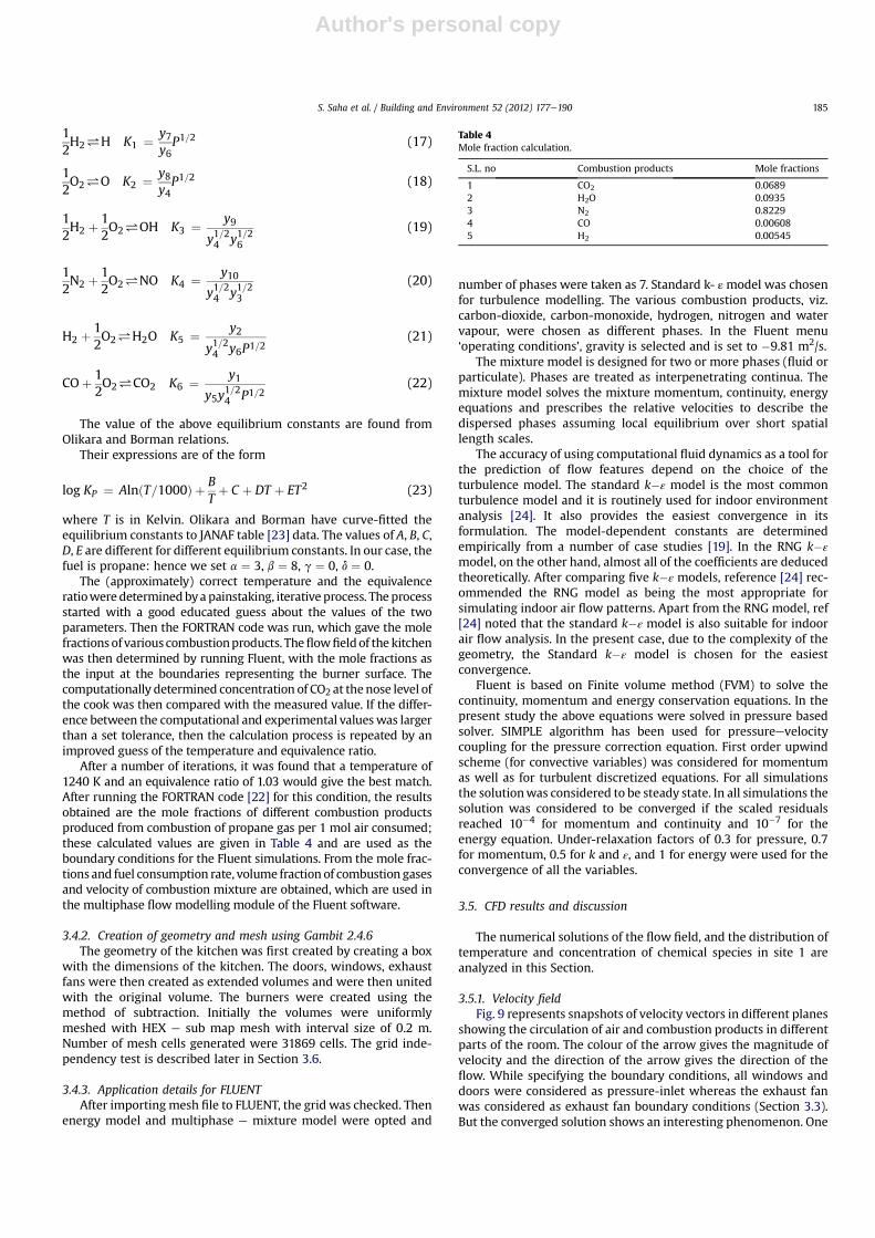
3.5.1. Velocity fieldFig. 9 represents snapshots of velocity vectors in different planes

showing the circulation of air and combustion products in differentparts of the room. The colour of the arrow gives the magnitude ofvelocity and the direction of the arrow gives the direction of theflow. While specifying the boundary conditions, all windows anddoors were considered as pressure-inlet whereas the exhaust fanwas considered as exhaust fan boundary conditions (Section 3.3).But the converged solution shows an interesting phenomenon. One

Table 4Mole fraction calculation.

S.L. no Combustion products Mole fractions

1 CO2 0.06892 H2O 0.09353 N2 0.82294 CO 0.006085 H2 0.00545



can see from the plotted velocity vectors in Fig. 5 that air enters inthe kitchen through all doors and windows except the window atthe right corner. Air exits through the right corner window. Thisshows that specifying the boundary conditions at all windows anddoors as “pressure-inlet” in Fluent did not predetermine thedirection of flow through these openings. The converged solutionevolves such that the correct direction of velocity vectors is auto-matically achieved. A circulation is produced near the cooking areadue to the high temperature of combustion gases. Air is exhaustedthrough the exhaust fan.

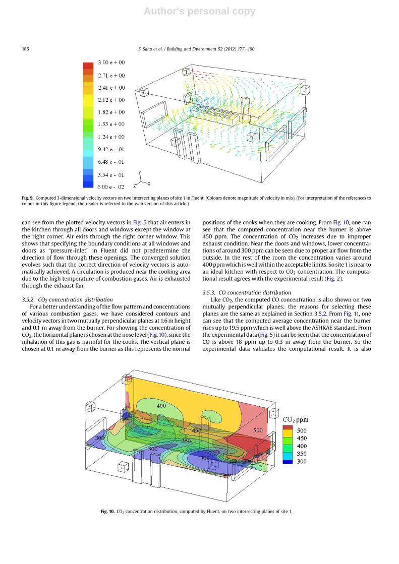
3.5.2. CO2 concentration distributionFor a better understandingof theflowpattern and concentrations

of various combustion gases, we have considered contours andvelocity vectors in twomutually perpendicular planes at 1.6mheightand 0.1 m away from the burner. For showing the concentration ofCO2, thehorizontal plane is chosenat thenose level (Fig.10), since theinhalation of this gas is harmful for the cooks. The vertical plane ischosen at 0.1 m away from the burner as this represents the normal

positions of the cooks when they are cooking. From Fig. 10, one cansee that the computed concentration near the burner is above450 ppm. The concentration of CO2 increases due to improperexhaust condition. Near the doors and windows, lower concentra-tions of around 300 ppm can be seen due to proper air flow from theoutside. In the rest of the room the concentration varies around400ppmwhich iswellwithin theacceptable limits. So site 1 is near toan ideal kitchen with respect to CO2 concentration. The computa-tional result agrees with the experimental result (Fig. 2).

3.5.3. CO concentration distributionLike CO2, the computed CO concentration is also shown on two

mutually perpendicular planes; the reasons for selecting theseplanes are the same as explained in Section 3.5.2. From Fig. 11, onecan see that the computed average concentration near the burnerrises up to 19.5 ppmwhich is well above the ASHRAE standard. Fromthe experimental data (Fig. 5) it can be seen that the concentration ofCO is above 18 ppm up to 0.3 m away from the burner. So theexperimental data validates the computational result. It is also

Fig. 9. Computed 3-dimensional velocity vectors on two intersecting planes of site 1 in Fluent. (Colours denote magnitude of velocity in m/s). (For interpretation of the references tocolour in this figure legend, the reader is referred to the web version of this article.)

Fig. 10. CO2 concentration distribution, computed by Fluent, on two intersecting planes of site 1.



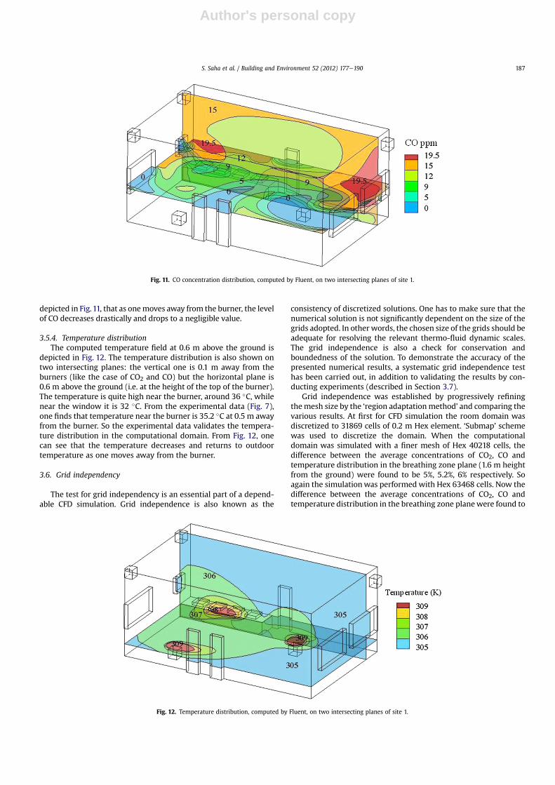
depicted in Fig.11, that as onemoves away from the burner, the levelof CO decreases drastically and drops to a negligible value.

3.5.4. Temperature distributionThe computed temperature field at 0.6 m above the ground is

depicted in Fig. 12. The temperature distribution is also shown ontwo intersecting planes: the vertical one is 0.1 m away from theburners (like the case of CO2 and CO) but the horizontal plane is0.6 m above the ground (i.e. at the height of the top of the burner).The temperature is quite high near the burner, around 36 �C, whilenear the window it is 32 �C. From the experimental data (Fig. 7),one finds that temperature near the burner is 35.2 �C at 0.5 m awayfrom the burner. So the experimental data validates the tempera-ture distribution in the computational domain. From Fig. 12, onecan see that the temperature decreases and returns to outdoortemperature as one moves away from the burner.

3.6. Grid independency

The test for grid independency is an essential part of a depend-able CFD simulation. Grid independence is also known as the

consistency of discretized solutions. One has to make sure that thenumerical solution is not significantly dependent on the size of thegrids adopted. In other words, the chosen size of the grids should beadequate for resolving the relevant thermo-fluid dynamic scales.The grid independence is also a check for conservation andboundedness of the solution. To demonstrate the accuracy of thepresented numerical results, a systematic grid independence testhas been carried out, in addition to validating the results by con-ducting experiments (described in Section 3.7).

Grid independence was established by progressively refiningthemesh size by the ‘region adaptationmethod’ and comparing thevarious results. At first for CFD simulation the room domain wasdiscretized to 31869 cells of 0.2 m Hex element. ‘Submap’ schemewas used to discretize the domain. When the computationaldomain was simulated with a finer mesh of Hex 40218 cells, thedifference between the average concentrations of CO2, CO andtemperature distribution in the breathing zone plane (1.6 m heightfrom the ground) were found to be 5%, 5.2%, 6% respectively. Soagain the simulationwas performed with Hex 63468 cells. Now thedifference between the average concentrations of CO2, CO andtemperature distribution in the breathing zone planewere found to

Fig. 11. CO concentration distribution, computed by Fluent, on two intersecting planes of site 1.

Fig. 12. Temperature distribution, computed by Fluent, on two intersecting planes of site 1.



be 0.1%, 0.85%, 1.55% respectively. It was decided that the gridindependence is achieved for the present purpose, and the gridwith Hex 63468 cells has therefore been adopted for numericalsimulations.

3.7. Comparison with full scale experiment

Finally, to further validate the accuracy of the numerical simu-lations undertaken, the predicted temperature field and thedistribution of chemical species are compared with the experi-mental values measured in the present work. A comparison of thesimulated and measured CO2, CO concentrations and temperaturefrom distance 0.1 m to 0.5 m away from the burner in the breathingzone plane (1.6 m from the ground) are presented in Table 5.Distance 0.1 m to 0.5 m away from the burner is considered herebecause this represents the main cooking area which is our regionof interest. For CO2 and CO concentration and temperature distri-bution fairly good agreement was found, though the experimentgave slightly higher concentrations and temperature.

This difference may have been caused by the measurementerrors, e.g. the data were not taken at a true steady state. Basicallythere is no real steady state for such a kitchen because the ambientconditions were continuously changing while in the simulation theaveraged ambient conditions were used. The flow rate through theburner is also varied in the experimental condition (as the cooksadjusted the burners depending on the various stages of a cookingprocess). The experimental data also changes with the time-dependent use of various kitchen appliances. (For example, it isfound that the species concentrations changed as the cooks movedthe ladle to stir the cooking materials in large pans). The effects ofmetabolism and activities of the workers of the kitchen are also notincorporated in the computational modelling. The discrepanciesfound here between CFD simulation and experimental observationmay also have resulted from insufficiently detailed representationof other boundary conditions. It may be possible to further improveCFD results by using a more refined representation of otherboundary conditions, such as wall temperature, velocity profile atdoors and windows. In addition more sophisticated treatment ofturbulence, wall effects and finer grid near the burner may alsoimprove CFD performances.

4. Theoretical studies of one improved design of the site 1

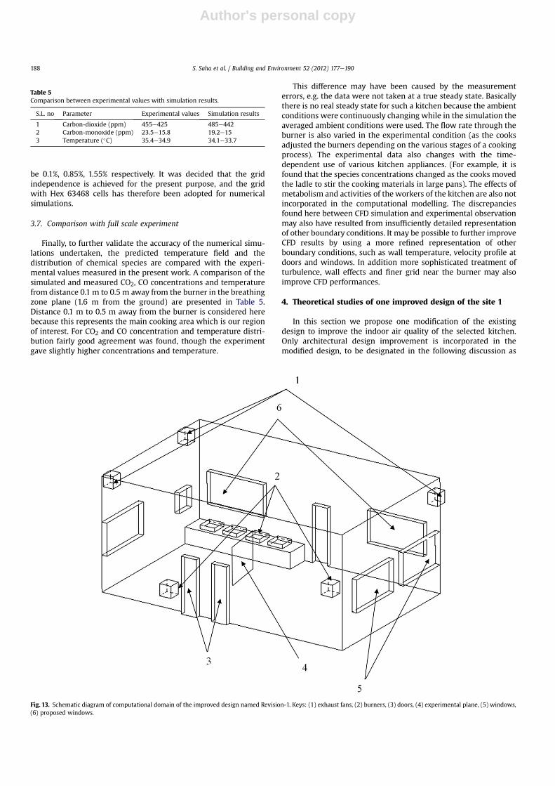
In this section we propose one modification of the existingdesign to improve the indoor air quality of the selected kitchen.Only architectural design improvement is incorporated in themodified design, to be designated in the following discussion as

Table 5Comparison between experimental values with simulation results.

S.L. no Parameter Experimental values Simulation results

1 Carbon-dioxide (ppm) 455e425 485e4422 Carbon-monoxide (ppm) 23.5e15.8 19.2e153 Temperature (�C) 35.4e34.9 34.1e33.7

Fig. 13. Schematic diagram of computational domain of the improved design named Revision-1. Keys: (1) exhaust fans, (2) burners, (3) doors, (4) experimental plane, (5) windows,(6) proposed windows.



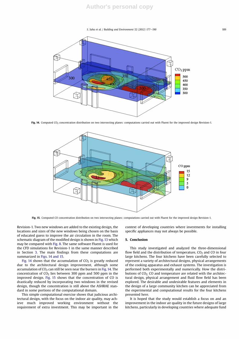
Revision-1. Two newwindows are added to the existing design, thelocations and sizes of the new windows being chosen on the basisof educated guess to improve the air circulation in the room. Theschematic diagram of the modified design is shown in Fig. 13 whichmay be compared with Fig. 8. The same software Fluent is used forthe CFD simulations for Revision-1 in the same manner describedin Section 3. The main findings from these computations aresummarized in Figs. 14 and 15.

Fig. 14 shows that the accumulation of CO2 is greatly reduceddue to the architectural design improvement, although someaccumulation of CO2 can still be seen near the burners in Fig.14. Theconcentration of CO2 lies between 300 ppm and 500 ppm in theimproved design. Fig. 15 shows that the concentration of CO isdrastically reduced by incorporating two windows in the reviseddesign, though the concentration is still above the ASHRAE stan-dard in some portions of the computational domain.

This simple computational exercise shows that judicious archi-tectural design, with the focus on the indoor air quality, may ach-ieve much improved working environment without therequirement of extra investment. This may be important in the

context of developing countries where investments for installingspecific appliances may not always be possible.

5. Conclusion

This study investigated and analyzed the three-dimensionalflow field and the distribution of temperature, CO2 and CO in fourlarge kitchens. The four kitchens have been carefully selected torepresent a variety of architectural designs, physical arrangementsof the cooking apparatus and exhaust systems. The investigation isperformed both experimentally and numerically. How the distri-butions of CO2, CO and temperature are related with the architec-tural design, physical arrangement and fluid flow field has beenexplored. The desirable and undesirable features and elements inthe design of a large community kitchen can be appreciated fromthe experimental and computational results for the four kitchenspresented here.

It is hoped that the study would establish a focus on and animprovement in the indoor air quality in the future designs of largekitchens, particularly in developing countries where adequate fund

Fig. 14. Computed CO2 concentration distribution on two intersecting planes: computations carried out with Fluent for the improved design Revision-1.

Fig. 15. Computed CO concentration distribution on two intersecting planes: computations carried out with Fluent for the improved design Revision-1.



for installing specific appliances may not always be available. Acomputational study summarized in Section 4 shows possible greatimprovement in indoor air quality for relatively modest alterationin the architectural design. The present experimental studydescribed in Section 2 shows that the indoor air quality of site 4 andsite 1 is close to an acceptable standard, but this is achieved in twodifferent ways. In site 4, local exhaust ventilation (LEV) systems foreach burner are responsible, whereas it is the general or dilutionventilation system and the large size of site 1 that achieve thedesired effect.

The experiments for the present study were carried out in situduring normal operational hours without disrupting the activitiesof the cooks and support staff. This makes the experimental dataparticularly useful for designing and assessing similar kitchens. Theexperimental results also reveal several subtle flow physics. Forexample, Fig. 5 shows the build-up of obnoxious gases near thesuction hood (a cook’s normal position of the nose should thereforebe away from this zone), the disparity in the emissions from thetwo burners shown in Fig. 6 inform us about the importance of theburner condition in maintaining indoor air quality, Fig. 7 revealshow an improperly designed ventilation system may blow hotobnoxious gases towards the cooks.

A computational procedure for determining the three-dimensional distribution of temperature and hazardous gases(such as CO2 and CO) inside an operational kitchen has beenformulated in the present study. The task is difficult because ofcomplex three-dimensional features of the computational geom-etry and complex sets of boundary conditions. A computationalmethod has been developed here for determining the volumefractions of CO2 and CO at the outlet of the burners that can be usedas the input boundary conditions of the CFD flow solver (such asFluent). The CFD simulations performed in the present work agreewell with the experimental results for the selected site 1. This directvalidation by comparing with present experimental results ob-tained in the same site gives confidence in the computationalprocedure devised here.

References

[1] Thiebaud HP, Knize MG, Kuzmicky PA, Hsieh DP, Felton JS. Airbone mutagensproduced by frying beef, pork and a soy-based food. Food Chem Toxicol 1995;33(10):821e8.

[2] Vainiotalo S, Matveinen K. Cooking fumes as a hygienic problem in the foodand catering industries. Am Ind Hyg Assoc J 1993;54(7):376e82.

[3] Guha A. A unified Eulerian theory of turbulent deposition to smooth andrough surfaces. J Aerosol Sci 1997;28(8):1517e37.

[4] Guha A. Transport and deposition of particles in turbulent and laminar flow.Ann Rev Fluid Mech 2008;40(1):311e41.

[5] Ng TP, Hui KP, Tan WC. Respiratory symptoms and lung function effectsof domestic exposure to tobacco smoke and cooking by gas in non-smoking Women in Singapore. J Epidemiol Community Health 1993;47(6):454e8.

[6] Li Y, Delsante A. Derivation of capture efficiency of kitchen range hoods ina confined space. Build Environ 1996;31(5):461e8.

[7] Khan JA, Feigley CE, Lee E, Ahmed MR, Tamanna S. Effects of inlet and exhaustlocations and emitted gas density on indoor air contaminant concentrations.Build Environ 2006;41(1):851e63.

[8] Chung KC, Hsu SP. Effect of ventilation pattern on room air and contaminantdistribution. Build Environ 2001;36(1):989e98.

[9] Srebic J, Vukorvic V, He G, Yang X. CFD boundary conditions for contaminantdispersion, heat transfer and air flow simulations around human occupants inIndoor environments. Build Environ 2008;43(1):294e303.

[10] Chiang CM, Lai CM, Chou PC, Li YY. The influence of an architectural designalternative (transoms) on indoor air environment in conventional kitchens inTaiwan. Build Environ 2000;35(1):579e85.

[11] Reggio M, Abanto J. Numerical investigation of the flow in a kitchen hoodsystem. Build Environ 2006;41(1):288e96.

[12] Lee E, Feigely C, Khan J. An investigation of air inlet velocity in simulating thedispersion of indoor contaminants via computational fluid dynamics. AnnOccup Hyg 2002;46(8):701e12.

[13] Atlanta GA. ASHRAE STANDARD 62-1982: ventilation for acceptable airquality. American Society of Heating, Refrigerating and Air ConditioningEngineers, Inc.; 1989.

[14] Burgess WA, Ellenbecker MJ, Treitman RD. Ventilation for control of the workenvironment. 2nd ed. New York: John Willey & Sons; 2004.

[15] Mannual for IAQ-CALC indoor air quality meter. 500 Cardigan Road, ShoreView, M.W 55126, USA: TSI Incorporated; August 2008.

[16] Aerias, Air Quality Sciences, IAQ resource centre.[17] Quinn P, Arnold DT. Environmental health fact sheet. Springfield, Illinois

62701: Illinois Department of Public Health; 2010.[18] Fluent 6.3.26, user guide. Fluent Inc; 2006.[19] Lee C, Lim K. A numerical study on the characteristics of flow field, temper-

ature and concentration distribution according to changing the shape ofseparation plate of kitchen hood system. Energy Build 2008;40(1):175e84.

[20] Daly BB. Woods practical guide to fan engineering. 3rd ed. Colchester: Woodsof Colchester Limited; 1978.

[21] Gambit 2.4.6, user guide. Fluent Inc; 2010.[22] Ferguson CR. Internal combustion engines. 1st ed. New York: John Willey &

Sons; 1986.[23] Chase MW, Curnutt JL, Hu AT, Prophet H, Syverud AN, Walker LC. JANAF

thermochemical tables, 1974 Supplement. Thermal Research, The Dowchemical company, Midland, Michigan 48640.

[24] Chen Q. Comparison of different k�εmodels for indoor air flow computations.Numer Heat Transfer 1995;28(B):353e69.

Nomenclature

cp: Specific heat at constant pressureK: Thermal Conductivityk: Turbulent kinetic energyN: Total number of molesP: PressureSu: Source termT: Temperaturev!dr;p: Drift velocity for secondary phase pVi: Number of molesv!m: Mass averaged velocityyi: Mole fractionap: Volume fraction of secondary phaseb1: Thermal expansion coefficientf: Equivalence ratiol: Source term in energy equationm: Dynamic viscositymt: Turbulent viscosityr: Densityrm: Mixture densitysij: Shear stressε: Dissipation energy˛: The molar fuel-air ratio

Subscriptsa: Number of Carbon atomsb: Number of Hydrogen atomsg: Number of Oxygen atomsd: Number of Nitrogen atomsi: Phase number (Eq. (16))p: Secondary phase (Eq. (6))


experimental and computational investigation of indoor air quality

Documents