experimental and computational study of vascular access for
TRANSCRIPT

Experimentele en computationele studievan vaattoegang voor hemodialyse
Experimental and Computational Studyof Vascular Access for Hemodialysis
Koen Van Canneyt
Promotoren: prof. dr. ir. P. Verdonck, prof. dr. ir. S. ElootProefschrift ingediend tot het behalen van de graad van Doctor in de Ingenieurswetenschappen: Biomedische Ingenieurstechnieken
Vakgroep Civiele TechniekVoorzitter: prof. dr. ir. J. De RouckFaculteit Ingenieurswetenschappen en ArchitectuurAcademiejaar 2012 - 2013

ISBN 978-90-8578-537-8NUR 954Wettelijk depot: D/2012/10.500/63

Supervisors:
Prof.dr.ir. Pascal VerdonckProf.dr.ir. Sunny Eloot
Research lab:
Bio�uid, Tissue and Solid Mechanics for Medical Applications (bioMMeda)Institute Biomedical Technology (IBiTech)Ghent University (UGent)De Pintelaan 185 - Block B9000 GentBelgium
Members of the exam committee:
Chairman:Prof.dr.ir. Hendrik Van Landeghem Faculty of Engineering and Architecture,
UGentSecretary:Prof.dr.ir Patrick Segers Faculty of Engineering and Architecture,
UGentReading committee:Prof.dr.ir. Cécile Legallais Faculty of Engineering, Université de
Technology de Compiègne, FranceDr. Nils Planken Department of Radiology, Academic
Medical Center Amsterdam, the Nether-lands
Dr. Jan Tordoir Department of Surgery, Maastricht Uni-versity Medical Center, the Netherlands
Prof.dr.ir. Frans van de Vosse Department of Biomedical Engineering,Technical University Eindhoven, the Ne-therlands
Prof.dr.ir. Jan Vierendeels Faculty of Engineering and Achitecture,UGent
Other members:Prof.dr.ir. Pascal Verdonck Faculty of Engineering and Architecture,
UGentProf.dr.ir. Sunny Eloot Faculty of Medicine and Health Science,
UGent
�is research was funded by Ghent University (appointment as assistant academicsta�) and by the European Commission 7th framework program (FP7-2007-2013:ARCH, Project n.224390).


SamenvattingSummary
iii


Samenvatting
Deel 1: Klinische achtergrond, hulpmiddelen en complicaties
Deel 1 biedt aan de lezer de nodige klinische achtergrond om de studies, dielater aan bod komen, te kunnen kaderen. Na een korte beschrijving van hetcardiovasculaire stelsel, de nieren en de bloedvaten in de bovenste ledema-ten, wordt dieper ingegaan op nierfalen, de nood voor een vaattoegang entot slot de drie types vaattoegangen.
Van nierfalen tot de nood voor een vaattoegang
Wanneer een patiënt lijdt aan terminaal nierfalen, moeten de functies van denieren overgenomen worden. Het ontvangen van een nier via transplantatieis de ideale vervangtherapie. Voor patiënten op de transplantatiewachtlijst,of patiënten die niet geschikt zijn als orgaanontvanger, bestaan er twee op-ties: peritoneaaldialyse of hemodialyse.Bij peritoneaaldialyse wordt een dialysaat (electrolyten oplossing) gra-
vitair in de buikholte gebracht via een peritonale katheter en werkt het sterkdoorbloede buikvlies (peritoneum) als membraan om de afvalsto�en uit hetbloed in het dialysaat te brengen. Na enkele uren laat men het ‘vuile’ dia-lysaat gravitair wegstromen uit de buik. Dit gebeurt meerdere keren perdag manueel of ’s nachts automatisch. Slechts 5-10% van de dialysepatiëntenmaakt gebruik van die techniek.De meest voorkomende vervangtherapie is hemodialyse, met ongeveer
een half miljoen patienten alleen al in Europa. Bij hemodialyse stroomt hetbloed van de patiënt extracorporeel door een kunstnier, een kunstmatig or-gaan. In die kunstnier wordt het bloed gezuiverd (di�usie en convectie) enwordt het overtollig water uit de patiënt onttrokken (ultra�ltratie). Omdatde patiënten niet 24u/24u zouden moeten verbonden blijven aan het he-modialysetoestel, moet het �lteren in de kunstnier e�ciënt gebeuren. Hetbloed van de patiënt moet daarom, tijdens de dialysesessie (meestal 3-4 u,3x per week), met een relatief hoog debiet (300-400ml/min) uit het lichaam
v

Samenvatting
stromen, door de kunstnier en terug naar de patiënt. Er moet dus een vaat-toegang gecreëerd worden die deze hoge debieten kan garanderen, die fre-quent bruikbaar is en die zoweinigmogelijk complicaties veroorzaakt. Hier-voor bestaan er drie mogelijkheden: een arterio-veneuze �stel, een arterio-veneuze gre�e en een centraal veneuze katheter.
Arterio-veneuze �stel (AVF)
Een arterio-veneuze �stel (AVF) is een directe verbinding tussen een arte-rie (slagader) en een vene (ader). Hierbij naait een (vaat)chirurg het hoge-druk-arteriële-systeem aan het lage-druk-veneuze-systeem. Die �stel wordtmeestal in de arm, bij voorkeur in de onderarm, aangelegd, door de veneop de zijkant van de arterie te naaien. De verbinding zelf noemt men deanastomose. De �stelcreatie zorgt dus voor een bypass van het haarvaten-systeem in de hand (een soort kortsluiting) en voor een hoog debiet doorde arm. Waar in de arm normaalgezien debieten van maximaal 100ml/minaanwezig zijn, kan dat postoperatief 10-20 keer hoger zijn.Door de verhoging van druk en debiet in de vene, wordt die vene groter
en verstevigt de wand. Dat proces noemt men maturatie en is noodzakelijkom ongeveer 6 weken na de operatie de vene te kunnen aanprikken meteen arteriële (aanzuig) en een veneuze (terugvoer) dialysenaald. In 25-45%van de gevallen faalt dit maturatieproces echter. Eens de �stel gematureerdis, is de meest voorkomende complicatie het vernauwen van de bloedvaten.Die stenosevorming vermindert het bloeddebiet door de �stel, waardoor dee�ciëntie van de hemodialysebehandeling sterk vermindert. Vooral dezecomplicatie zorgt ervoor dat ongeveer 50% van de �stels binnen het jaar eenradiologische of chirurgische interventie nodig hebben om hun werking tegaranderen.Daarnaast is het ook mogelijk dat er een te groot debiet door de �stel
anastomose stroomt en dat de drukval van arterie naar vene te laag is. Hier-bij komt de doorbloeding van de distale delen (stroomafwaarts, meer speci-�ek, de hand) in het gedrang. Deze ischemie kan leiden tot necrose van hetweefsel. Ook een overload van het hart, dat het verhoogde debiet door dearm, als surplus, moet aanleveren, is hierbij een ernstige complicatie.Er is aangetoond dat een �stel deminste complicaties teweegbrengt, ver-
geleken met de andere vaattoegangen. Daarom hoort dit type vaattoegangde eerste keuze te zijn bij een hemodialysepatiënt.
Arterio-veneuze gre�e (AVG)
De arterio-veneuze gre�e (AVG) is een variant van de AVF. Bij een AVGwordt onderhuids een kunstmatig textiel buisje genaaid tussen de arterie
vi

Deel 2: Ingenieurshulpmiddelen
en de vene. Deze vaattoegang wordt meestal toegepast bij patiënten wiensvenen van een mindere kwaliteit zijn. In het geval van een gre�e, wordende dialysenaalden dan ook in de gre�e zelf geprikt. De meest voorkomendecomplicatie hierbij is stenosevorming aan de veneuze anastomose en in debloedafvoerende vene. Algemeen kan aangenomen worden dat er bij gre�emeer interventies nodig zijn om de vaattoegang goed werkend te houdendan bij een �stel.
Centraal veneuze katheter (CVC)
Een centraal veneuze katheter (‘central venous catheter’, CVC) bestaat uit éénof twee lumens (buisjes) en wordt ingebracht in een vene die naar de venacava superior of de rechter voorkamer van het hart loopt. Deze katheterwordt, meestal ter hoogte van het sleutelbeen, naar buiten geleid zodat hijverbonden kan wordenmet het dialysetoestel. Het gebruik van katheters alspermanente vaattoegang wordt afgeraden door het veelvuldig voorkomenvan complicaties zoals infectie en thrombose. De CVC wordt echter wel ge-bruikt bij hemodialyse tijdens het matureren van een �stel of wanneer geenenkele �stel of gre�e meer kan aangelegd worden.Er is een grote verscheidenheid aan beschikbare katheter designs. Van
het ‘shotgun’-ontwerp (terugvoer-lumen langer dan aanzuig-lumen), oversymmetrische ontwerpen, tot ontwerpen waar beide lumens los van elkaarhangen (‘split’-ontwerp). Elk van die designs hee� voor- en nadelen.
Deel 2: Ingenieurshulpmiddelen
Deel 2 behandelt enkele (ingenieur-)technische onderwerpen, ter verdui-delijking van de gebruikte methodes in de uitgewerkte studies. Vooreerstwordt het Europees ARCH-project kort toegelicht. Enkele studies die be-schreven worden in dit manuscript maken deel uit van dat Europees pro-ject. Enkele andere studies zijn gebaseerd op data uit het ARCH-onderzoek.Daarna wordt de basis van de vloeistofmechanica beschreven: de algemenevloeistofeigenschappen (dichtheid, viscositeit, . . . ), de behoudswetten en despeci�eke karakteristieken van vloeistof in beweging. Om deze ingenieurs-achtergrond te vervolledigen worden de gebruikte technieken, zowel com-putationeel als experimenteel, ingeleid.
Computationele methodes
Vooreerst werd gebruik gemaakt van computational �uid dynamics (CFD,numerieke stromingsleer) berekeningen. Die techniek bestaat erin een vo-lume eerst onder te verdelen in zeer kleine cellen (‘meshen’). Daarnaworden
vii

Samenvatting
de wetten van behoud van massa en momentum berekend in elke cel om zomet een iteratief proces de stroming in het volledige volume te begroten envisualiseren. Daarnaast laat deze techniek ook toe om schuifspanningen teberekenen.Een tweede computationele methode die in dit werk gebruikt werd, is
kinetischemodellering. Deze techniek verdeelt het lichaam in virtuele com-partimenten om het inwendige massatransport te kwanti�ceren.
Experimentele methodes
In het experimenteel (in vitro) gedeelte van dit onderzoek werd gebruik ge-maakt van siliconemodellen van de bloedvaten in de arm. Die modellenwerden aangesloten op gestuurde pompen en geconnecteerd met drukva-ten, reservoirs en weerstanden stroomafwaarts. Nadat fysiologische druk-en stromingsrandvoorwaarden gecreëerd werden, konden zowel de disten-sie (diameter verandering ten gevolge van drukgolf) als de stromings- endrukpro�elen nauwkeurig opgemeten worden. De bekomen data diendedeels als input van de computermodellen, en deels om de output van decomputermodellen te veri�ëren.Voor het experimenteel gedeelte werd ook gebruik gemaakt van Particle
Image Velocimetry (PIV). Hierbij wordt op een perfect transparant modeleen laser vlak aangebracht. Door het model stroomt een vloeistof waarinkleine re�ecterende deeltjes, partikels, zijn aangebracht. Een camera regi-streert de deeltjes die door het laser-verlichte gebied bewegen. Door verge-lijking van opeenvolgende beelden kunnen dan lokale snelheden berekendworden.
Deel 3: Studies over AVF’s
Computationele studie van stroming in een AVF anastomose
Tot op heden is er weinig interesse voor de geometrie van de anastomosezelf, hoewel dit een cruciaal onderdeel is van het stromingspad en er tot 95%van het bloed in de arm moet door stromen. In de studie beschreven inhoofdstuk 10 gaan we dieper in op de stroming in de arterio-veneuze ana-stomose en beschrijven we de invloed van de grootte van die verbindingen van de hoek tussen arterie en vene op zowel het debiet als de drukver-deling. We creëerden 11 verschillende computermodellen van een arterie,waarop langs de zijkant een vene is geconnecteerd, en waarbij de anasto-mose grootte varieerde tussen de 12.6 en 23.6mm2 en de anastomose hoektussen de 27○en 90○. Met CFD-berekeningen werd de stroming in deze ver-eenvoudigde AVF-modellen geanalyseerd.
viii

Deel 3: Studies over AVF’s
In een eerste luik hebben we een uitstroom debietsverdeling vastgelegden het instroom debiet gevarieerd tussen de 600-1200ml/min. We kondenaantonen dat de drukval over de anastomose (drukverschil tussen arteriëleen veneuze druk, de ‘weerstand’) kwadratisch stijgt met een groter wordenddebiet en dat de drukval kleiner wordt als de anastomose vergroot of als dehoek wijder wordt dan 43○.In een tweede luik hebben we de drukken aan in- en uitlaat vastgezet en
opnieuw de 11 verschillende modellen doorgerekend. Naar analogie met debevindingen uit het eerste deel, merkten we nu dat het instroomdebiet steegals de anastomose oppervlakte of hoek groter werden. Omdat de drukvalover de anastomose zodanig daalde, werd er zelfs bloed vanuit het distaledeel van de arterie (van de hand) aangezogen naar de vene. Dit laatste kanklinisch leiden tot distale hypoperfusie of zelfs ischemie.Deze studie toonde duidelijk aan dat de grootte en de hoek van de ana-
stomose zeer bepalend zijn voor de stroming in de �stel. Omdat een te kleineanastomose meestal maturatie verhindert, wordt snel overgeschakeld naareen (te) grote anastomose. Het gebrek aan interesse voor de geometrie vande anastomose lijkt echter onterecht. Een verandering van 2mm lengte bij-voorbeeld kan leiden tot een verhoging van de drukval met 30%.
Experimentele validatie
Binnen het Europese project ARCH (hoofdstuk 7) werd een computerpro-gramma ontwikkeld dat aan de hand van patiënt-speci�eke, preoperatieve,medische beelden en gegevens, de direct postoperatieve debieten en druk-ken in arteries en venen kan voorspellen. Hierbij kan reeds vóór de aanlegvan de �stel, patiënt-speci�ek, de optimale �stellocatie gekozen worden. Al-vorens het computermodel in de klinische praktijk kan getest en geoptima-liseerd worden, was het aangeraden om de nauwkeurigheid van het modelen de achterliggende fysica rigoureus te veri�ëren. Deze veri�catie was mo-gelijk aan de hand van experimentele validatiestudies (hoofdstuk 11). Hierbijwerd een model gebouwd dat gebaseerd is op patiënt-speci�eke data, werddit experimentele model met de computer nagebouwd en werden resultatenvan het experiment en het computermodel vergeleken.De eerste experimentele setup, besproken in sectie 11.1, bestond uit een
pomp (cfr. het hart) gekoppeld aan een siliconen model van zowel de aorta,de belangrijkste arteriën in de arm, een AVF ter hoogte van de pols, als en-kele venen. De geometrie (lengtes en diameters) en de distensie werdenopgemeten en overgezet naar het numerieke pulse wave propagationmodel(een 1D representatie van een vaatstructuur voor het berekenen van druk- en
ix

Samenvatting
debietsgolven). Wematen druk- en debietsgolven op 11 plaatsen experimen-teel op en vergeleken deze met de computationele resultaten. Het was dui-delijk dat het computermodel de gemiddelde druk en het gemiddelde debietaccuraat kon simuleren. De golfvormen zelf waren echter minder gedemptdan in het experimentele model. Dit laatste wellicht door het ontbreken vanvisco-elasticiteit in het computermodel.Verder voerden we een analyse uit rond de precisie van de outputwaar-
den, rekening houdend met de onnauwkeurigheden van de inputdata. Ditwerd uitgevoerd aan de hand vanMonte Carlo simulaties waarbij elke para-meter, binnen een opgegeven nauwkeurigheid, 5000 keer werd veranderd.Hieruit bleek duidelijk dat de onzekerheid op de gemeten waarden (vb. dia-meter arterie ± 10%) sterk kon teruggevonden worden in een onzekerheidop de gesimuleerde output. Dus het reduceren van de onzekerheid op deinputdata, hee� een grote invloed op de onzekerheid van de computer re-sultaten. Deze kennismoet in rekening gebracht wordenwanneer hetmodelklinisch geïmplementeerd wordt.Een tweede validatiestudie, besproken in sectie 11.2, maakte gebruik van
een patiënt-speci�ek model van een arterio-veneuze �stel. Hierbij werd destroming gevisualiseerd ter hoogte van de anastomose doormiddel van PIV-metingen. Daarnaast hebben we de drukval over de anastomose (van arterietot vene) experimenteel opgemeten voor meer dan 200 verschillende debie-ten. We vonden een goede overeenkomst tussen het stromingsbeeld gege-nereerd door de PIV-metingen en dat gesimuleerd door het CFD-model.Daarnaast vonden we opnieuw een kwadratisch verband tussen debiet endrukval en kwam dit verband goed overeen met de resultaten van de com-puterberekeningen.Er kan dus gesteld worden dat, rekening houdend met een vastgestelde
onzekerheid, beide computermodellen betrouwbare resultaten geven en duskunnen ingezet worden om patiënt-speci�eke hemodynamica nauwkeurigte simuleren.
Diagnose methodes
In hoofdstuk 12werden twee methodes bestudeerd die de arts kan helpen bijde diagnostiek rond AV-�stels.Ten eerste hebben we in sectie 12.1 een methode uitgewerkt die in staat
is stenoses te detecteren met een diameterreductie van 25-50%. De hui-dige methodes zijn meestal gebaseerd op drukvalverhoging of debietsver-mindering en kunnen slechts vernauwingen detecteren van ongeveer 70%diameterreductie (≈ 90% doorstroomoppervlakte reductie). De hier bestu-deerde methode maakt echter geen gebruik van de gemiddelde druk maar
x

Deel 3: Studies over AVF’s
van de pulsdruk (maximale minminimale druk tijdens een hartslag cyclus).We toonden aan, via een silicone experimenteel model, dat stenoses in eenvroegtijdig stadium kunnen gedetecteerd worden aan de hand van drukgol-ven geregistreerd aan de dialysenaald. Deze polsdruk analyse (pulse pressureanalysis (PPA)) bleek onafhankelijk van debiet en hartslag. Klinische stu-dies moeten deze experimentele resultaten natuurlijk bevestigen, maar dezelage-kostenmethode biedt goede perspectieven.Een tweede diagnosemethode die onder de loep werd genomen is de
pulsed wave Doppler ultrasound (PWD-US) debietsmeting (sectie 12.2). BijPWD-US wordt de gemiddelde snelheid [m/s] in een doorsnede berekenden vermenigvuldigd met de oppervlakte van de doorsnede [m2] om zo hetdebiet [m3/s of ml/min] te bekomen. Deze methode kan bijvoorbeeld ge-bruiktworden omdirect postoperatieve debietsmetingen uit te voeren. Dezemetingen blijken namelijk een voorspellend karakter te hebben rond het sla-gen van de �stelmaturatie. Een e�ciënte en betrouwbare methode om de-bieten te meten is dus nodig.Het bleek dat men met PWD-US (echogra�e) de bloedsnelheid, in het
centrum van een bloedvat, in de richting van de probe, nauwkeurig kan be-palen. Wanneer echter wordt overgegaan naar debietvoorspellingen, blij-ken er grote onnauwkeurigheden in de metingen te ontstaan. Een patiënt-speci�ekCFD-modelwerd opgebouwd, en de ultrasone spectrawerden com-putationeel gegenereerd. We analyseerden zowel een pre- als een postope-ratief model, beiden ter hoogte van de elleboog en van de pols.We toonden aan dat er, bij complexe stroming, reeds fouten worden ge-
ïntroduceerd wanneer de snelheid zoals opgepikt door de US-probe (in derichting van de probe) wordt omgezet naar de snelheid in de lengterichtingvan het bloedvat. Maar het werd vooral duidelijk dat de grootste onnauw-keurigheid wordt geïntroduceerd wanneer de snelheid in een punt (vb. cen-trum van het bloedvat, 0D) of op een lijn (over de volledige diameter vanhet bloedvat, 1D) wordt omgezet naar de gemiddelde snelheid in de door-stroomoppervlakte (2D). De vorm van het lokale snelheidspro�el is name-lijk volledig onbekend. We vergeleken aannames van parabolische pro�elen(Poiseuille stroming), vlakke pro�elen (plug stroming) en tijdsafhankelijkepro�elen (Womersley stroming).Er kon geconcludeerd worden dat er geen enkele aanname werkt in elk
van de situaties en dat er bij gebruik van PWD-US debietsdata rekeningmoet gehouden worden met zeer grote onnauwkeurigheden op de verkre-gen debietswaarden.
xi

Samenvatting
Deel 4: Studies over AVG’s
Helicale gre�e designs
Zoals vermeld is stenosevorming een veel voorkomende complicatie bij gref-fes. Deze vernauwingenworden veroorzaakt door neo-intimale hyperplasie.Dit ongecontroleerd groeien van cellen uit de intimalaag van de bloedvat-wand wordt gedreven door abnormale lokale stromingspatronen. In de li-teratuur staat beschreven dat fenomenen als lage gemiddelde wandschuif-spanning (lage time-averaged wall shear stress, TAWSS), sterk oscillerendewandschuifspanning (hoge oscillatory shear index, OSI) en hoge verblijfstijd(hoge relative residence time, RRT) deze neo-intimale hyperplasie induceren.Daarnaast is er beschreven dat stroming met veel wervels deze ongunstigehemodynamica reduceren.In hoofdstuk 13 hebben we de beschreven stromingsfenomenen bestu-
deerd in gre�esmet een spiraalvormig (helix) design, aan de hand vanCFD-simulaties. Er werden vijf verschillende helicale designs, parametrisch, ont-worpen (met torsielengtes van 17,5 tot 6 keer de gre�e diameter) en verge-leken met een rechte, conventionele gre�e. Uit de berekeningen, uitgevoerdmet hoge nauwkeurigheid, kon worden afgeleid dat het introduceren vaneen spiraalvorm (swirl) in het design van een gre�e leidt tot een meer com-plex stromingsbeeld en dat de zonesmet ongunstige hemodynamica geredu-ceerd worden. De graad van reductie bleek echter niet proportioneel met deingebrachte heliciteit en we kunnen aannemen dat de e�ectiviteit van dezegre�es dan ook casus per casus moet bekeken worden.
Deel 5: Studies over CVC’s
Computationele studie rond katheter met nieuw tipdesign
Bij het ontwerp van een katheter is het de bedoeling dat de recirculatie zolaag mogelijk is (eventueel zelfs bij omgekeerde connectie van de aanslui-tingen), dat het bloed niet stilstaat in de lumens (klontervorming) en dathet bloed zo weinig mogelijk wrijving ondervindt (beschadiging van rodebloedcellen, hemolyse).In hoofdstuk 14werd het ontwerp van een nieuwe katheter, met een sym-
metrische tip, onder de loep genomen. Een uitgebreide CFD-analyse toondeaan dat er een verwaarloosbare recirculatie optrad in de nieuwe VectorFlowkatheter. Dit werd zowel in een experimentele studie als in een studie opeen varkensmodel bevestigd. Daarnaast was het in de computationele stu-die mogelijk de stromingspatronen rond de tip te bestuderen en parameters
xii

Deel 5: Studies over CVC’s
rond klontervorming en hemolyse te analyseren en te vergelijken. De stro-mingsfenomenen en parameters bleken voor het nieuwe design vergelijk-baar met die bij reeds bestaande standaard ontwerpen. De studie toonde degrote potentie van de VectorFlow katheter, door het uitblijven van recircu-latie, en opent de deur voor verdere (pre-)klinische studies.
Computationele studie naar suboptimaal werkende katheters
Wanneer het gewenste dialysedebiet niet meer kan verkregen worden bij ge-bruik van een katheter met twee lumens, wordt ofwel verder gedialyseerdmet het verlaagde bloeddebiet of worden de aanzuigzijde (arteriële lumen)en de terugvoerzijde (veneuze lumen) omgekeerd geconnecteerd. Omdat demeeste katheters ontworpen zijn om in gewone werking zo weinig mogelijkgezuiverd bloed (uit veneuze lumen) terug aan te zuigen (via arteriële lu-men), recirculatie genaamd, zorgt een omkering van de connecties meestalwel voor een verhoogde recirculatie.In sectie 15.1 hebben we eerst bij een groep van 22 patiënten onderzocht
hoe e�ciënt de hemodialyse is als de connecties omgekeerd worden. Hier-uit bleek dat de e�ciëntie niet signi�cant verschilde bij gewone versus om-gekeerde connectie voor ureum, creatinine, beta-2-microglobulin (β2M) enfosfaat. Daarnaast werd een eerste mathematische model opgebouwd dooreen 1-compartiment kinetisch model te koppelen aan een dialysemodel. Destudie rond de klaring (afvoer) van ureum tijdens dialyse toonde aan dat erslechts een reductie van de e�ciëntie, op basis van de hoeveelheid verwij-derde stof, van 9.2% optrad bij een recirculatie van 10%.Om de vertraagde distributie van sto�en in het lichaam beter te kunnen
modelleren werd in sectie 15.2 het meer volledige 2-compartimenten kine-tisch model uitgewerkt. Hierbij werden vier verschillende opgeloste sto�enbestudeerd: ureum, methylguanidine, β2M en fosfaat. Hiermee werd aan-getoond dat in een standaard dialysesessie (4 uur), een katheter met éénlumen zorgt voor een minder e�ciënte dialyse vergeleken met een kathetermet twee lumens. Daarnaast werd duidelijk dat het omkeren van de lijnenbij een suboptimaal werkende katheter beter is dan het blijven dialyseren incorrecte connectie maar met verminderd debiet.Vertrekkend van het 2-compartimenten kinetisch model, zijn we in sec-
tie 15.3 dieper ingegaan op een verlengde dialysesessie (8 uur), die vooral ’snachts, zowel in dialysecentrum als thuis, kan plaatsvinden. Daardoor heb-ben ze vaak een lagere impact op het leven van de patiënt. Vooreerst vondenwe dat er in een 8 u dialyse, bij gelijke debieten, een verhoging van de dia-lysee�ciëntie plaatsvond ten opzichte van 4 u dialyse. De verwijdering vande opgeloste sto�en was, door het vertraagde transport in het lichaam, ech-ter niet verdubbeld.
xiii

Samenvatting
Om de nachtrust van de patiënten te bewaren (minder opstaan om con-centraatzakken te verwisselen en minder alarms) en de kost van water on-der controle te houden, zou dialyse met een gehalveerd debiet aangewezenkunnen zijn. Voor deze lange trage dialyse vonden we een e�ciëntie verge-lijkbaar met standaard 4 u dialyse. Ten slotte werd nog de optie bestudeerdwaarbij de patiënt zichzelf met één naald aanprikt (in plaats van twee) ineen arterio-veneuze �stel of waarbij er een katheter met enkel lumen ge-bruikt werd. Hierbij vonden we een verhoogde e�ciëntie ten opzichte vande standaard 4 u dialyse.
Deel 6: Algemene conclusies
Door het uitvoeren van de verschillende computationele en experimentelestudies, komen we tot volgende stellingen:• Bij een AVF moet de grootste drukval over de anastomose liggen.• Het gebruik van een helix vorm in het ontwerp van een AVG intro-duceert een complexer stromingsveld en reduceert de zones met on-gunstige hemodynamica, maar doet deze echter niet verdwijnen.
• De VectorFlow CVC is een veelbelovende katheter door de verwaar-loosbare recirculatie.
• Het pulse wave propagation model en het numerieke stromingsleer-pakket voor hoge debieten, ontwikkeld in het ARCH-project, zijn ex-perimenteel gevalideerd en kunnen gebruikt worden voor implemen-tatie in de klinische praktijk.
• Experimenteel onderzoek vereist ervaren onderzoekers.• Het uitvoeren van polsdruk analyse aan de arteriële dialysenaald kanleiden tot het vroegtijdig detecteren van stenoses.
• Standaard pulsed wave Doppler ultrasoundmetingen leveren geen be-trouwbare waarde voor het bloeddebiet.
• Bij een slecht werkende dubbel lumen CVC tijdens standaard (4 u)dialyse moet het omkeren van de katheter connecties en behoud vanvoldoende debiet de voorkeur krijgen.
• Trage dialysemet een dubbel lumen CVC, of dialysemet een enkel lu-men CVC ofmet één naald in de AVF, zijn goede alternatieven tijdensdialyse met verlengde duur (8 h).
xiv

Summary
Part 1: Clinical background, devices and complications
�e �rst part provides the reader with the necessary clinical background tounderstand the conducted studies in this work. A�er a brief description ofthe cardio-vascular system, the kidneys and the blood vessels in the upperextremities, kidney failure, the need for a vascular access and the three typesof vascular access are discussed.
From a failing kidney to the need for a vascular access
If a patient su�ers from an end-stage renal disease (total kidney failure), thefunctions of the kidneys must be reproduced. Receiving a kidney transplantis the best replacement therapy. For patients on the transplant waiting listor patients not suitable as organ recipient, there are however two options:peritoneal dialysis or hemodialysis.During peritoneal dialysis, a dialysate (electrolyte solution) is brought,
by gravity, in the abdominal cavity via a peritoneal catheter.�e highly vas-cularized peritoneum acts as amembrane, bringing waste products from theblood into the dialysate. A�er a few hours, the spent dialysate is drained, bygravity, from the abdomen to a waste bag. �is sequence is repeated sev-eral times a day manually or at night automatically. Only 5-10% of dialysispatients make use of this technique.
�emost common renal replacement therapy is hemodialysis, withmorethan half-a-million patients in Europe. Within this therapy, the patient’sblood �ows extracorporally through an arti�cial kidney, an arti�cial organ.In an arti�cial kidney, the blood is puri�ed (convection and di�usion) andexcess water is removed from the patient (ultra�ltration). To avoid that thepatient should remain connected to the dialyzer 24/7, the treatment shouldhappen as e�cient as possible.�e patient’s blood should therefore, duringthe dialysis session (usually 3-4 h, 3/week), �owwith a relative high �ow rate(300-400ml/min) through the arti�cial kidney.�erefore, there is the needto create a vascular access which can provide these high �ow rates, which
xv

Summary
is frequently usable and which has a low complication rate.�ere are threepossibilities: an arterio-venous �stula, an arterio-venous gra� and a centralvenous catheter.
Arterio-venous �stula (AVF)
An arterio-venous �stula (AVF) is a direct connection between an arteryand a vein. A (vascular) surgeon sews the high-pressure arterial system tothe low-pressure venous system. �e �stula is mostly created in the arm,preferably in the lower arm, by connecting a vein to the side of an artery(end-to-side). �e connection itself is called the anastomosis. �e �stulacreation causes a bypass of the capillary system (sort of short circuit) andan increase in blood �ow through the arm. Normally, the �ow in the armis around 100ml/min, but a�er �stula creation this can increase by a factorten to twenty.Due to the increase in pressure and �ow, the vein enlarges and the vein
wall reinforces.�is process, called maturation, is required to puncture thevein, mostly starting 6-8 weeks a�er the surgery, with an arterial (suction)and venous (return) dialysis needle. However, failure to mature occurs in25-45% of the cases.Once the �stula matured, the narrowing of the vessels is the most com-
mon complication.�is stenosis formation reduces the blood �ow rate andinhibits an e�cient dialysis treatment.�is complication in particular, is re-sponsible for the fact that up to 50% of �stulas need a surgical or radiologicalintervention within the �rst year.In addition, a too high �ow rate and/or to low pressure drop over the
arterio-venous anastomosis o�en occur. Hereby, the blood circulation tothe distal part (downstream, more speci�cally the hand) is inhibited. �isdistal hypoperfusion syndrome can lead to ischemia and even necrosis ofthe tissue. Furthermore, the heart has to deliver this elevated blood �ow tothe arm and a cardiac overload can occur.It has been shown that the complication rate in �stulas is lower com-
pared to the other vascular access options.�erefore, an AVF should be the�rst option as vascular access.
Arterio-venous gra� (AVG)
An arterio-venous gra� (AVG) is a variant on an AVF. With a gra�, an ar-ti�cial textile tube is sewn, subcutaneously, between an artery and a vein.�is vascular access is usually used in patients with low quality veins. In thecase of a gra�, the dialysis needles are inserted in the gra� itself. �e mostcommon complication is stenosis formation at the venous anastomosis and
xvi

Part 2: Engineering tools
in the draining vein. �e number of vascular access interventions neededto maintain the gra�’s well functioning is higher compared to the necessaryinterventions associated with a �stula.
Central venous catheter (CVC)
A central venous catheter (CVC) consists of one or two lumens (tubes) andis inserted into a vein leading to the vena cava superior or the right atrium.�e catheter is brought, usually at the height of the collar bone, to the outsideto be able to be connected with the dialysis machine. �e use of cathetersas permanent vascular access is not recommended due to the frequent oc-currence of complications such as infection and thrombosis. �e CVC isnonetheless used for hemodialysis during the maturation of a �stula or if nomore �stula or gra� can be constructed.
�ere is a great variety in available catheter designs. From the ‘shotgun’design (return lumen longer than suction lumen), over symmetrical designsto designs where both lumens are separated (‘split’ design), each with theirown advantages and disadvantages.
Part 2: Engineering tools
In the second part, some engineering background is provided. �is shouldmake the methods, applied in the studies, more clear. First, the EuropeanARCH-project is brie�y explained.�is is because some studies in this dis-sertation were, on the one hand, part of this research project or, on the otherhand, rely on data from it. Next, the basic principles of �uid mechanics aredescribed, starting from the overall liquid properties (density, viscosity, . . . ),over the conservation laws, to speci�c characteristics of the �uid in motion.To complete this engineering background part, the used techniques, bothcomputational and experimental, are introduced.
Computational methods
Some computational studies were conducted based on computational �uiddynamics (CFD) calculations. In CFD, a volume has to be subdivided into alarge number small volume cells (‘meshing’).�en, in each cell, an iterativeprocedure is applied until the laws of conservation of mass and momentumresult in negligible residuals.�is allows us to visualize and analyze the �owin great detail. In addition, also shear stresses or blood residence times canbe calculated.
�e second computational method that was used in this work is kineticmodeling. �is technique virtually divides the body into several compart-ments to quantify the internal mass transport phenomena.
xvii

Summary
Experimental methods
Silicone models of the blood vessels in the arm were used during the exper-imental (in vitro) part of the research.�ese were connected to (controlled)pumps, (pressure) reservoirs and downstream resistances. When physiolog-ical pressure and �ow conditions were created, we couldmeasure distension(change in diameter due to pressure changes) and �ow and pressure pro�lesaccurately. �e obtained experimental data could partly serve as input forcomputer models and partly to verify the output generated by the computermodels.During the experimental studies, Particle Image Velocimetry (PIV) was
used as well. A thin laser sheet is applied on a transparent model and a liq-uid, seeded with small tracer particles, �ows through the model. A camerarecords the particles �owing through the illuminated region of interest.�elocations of the particles over consecutive images are compared to achievethe local velocity �eld.
Part 3: Studies on AVFs
Computational study on �ow in a AVF anastomosis
Although the anastomosis is a crucial element in the blood �ow path and90-95% of the blood �ow in the arm passes it, there is, in general, a signif-icant absence of interest in the geometry of the anastomosis. In the studydescribed in chapter 10, the �ow in the anastomosis region was assessed inmore detail and we described the impact of the size of the anastomosis, aswell as of the angle between vein and artery, on �ow rates and pressure dis-tribution.�erefore, we created 11 di�erent computational models of a veinconnected to the side of an artery with a varying anastomosis size (12.6-23.6mm2) and anastomosis angle (27-90○).�e �ow in these simpli�edAVFmodels was analyzed based on CFD-calculations.First, an out�ow distribution was �xed, while the in�ow �ow rate was
changed between 600 and 1200ml/min. We were able to show that the pres-sure drop over the anastomosis (arterial minus venous pressure) changesquadratically with the in�ow rate and decreases when the anastomosis sizeincreases or the angle gets wider then 43○.Later, we �xed the inlet and outlet pressures and recalculated all 11 CFD
models. In analogy with the conclusions from the �rst part, we found anincreased �ow rate when the anastomosis size or angle increased. Becausethe decrease in pressure drop over the anastomosis was very high, bloodwas ‘stolen’ by the vein from the distal artery (from the hand). �is ‘stealsyndrome’ can clinically lead to distal hypoperfusion or even ischemia.
xviii

Part 3: Studies on AVFs
�e study clearly showed that the anastomosis size and angle have a greatin�uence on the �ow�eld in the �stula. Because a too small anastomosis caninhibit the maturation process, physicians switch too fast to a (too) largeanastomosis.�e lack of interest concerning the geometry of the anastomo-sis seems, however, unfair. A change of, for example, 2mm in anastomosislength can lead to a pressure drop increase of 30%.
Experimental validation
Within the context of the European ARCH project (chapter 7), a compu-tational modeling framework was developed to predict direct postopera-tive �ow and pressure in both arteries and veins, based on patient-speci�c,preoperative, medical images and functional data. �e goal is to predict,patient-speci�cally, the optimal AVF anastomosis location. Before the test-ing and optimization of the model framework in clinical practice, it wasrecommended to rigorously verify the numerical model and the underly-ing physics.�is veri�cation was performed using experimental validation(chapter 11). First, an in vitromodel was built based on patient-speci�c data,second, the experimental model was reconstructed in the computer modeland, �nally, the experimental and computational results were compared.
�e �rst experimental setup we used, discussed in section 11.1, consistsof a pump (cf. the heart) coupled with a silicon model of the aorta, the mostimportant arteries in the arm, an AVF at the wrist and a basic venous circuit.�e geometry (lengths and diameters) and the distensibility were measuredand converted to the numerical pulse wave propagation model (a 1D rep-resentation of the vessel topology for the calculation of pressure and �owwaveforms). We obtained experimentally pressure and �ow waveforms on11 di�erent locations throughout the siliconmodel and compared these withthe computational results. It was clear that the computational model wasable to accurately simulate themean pressure and �ow rates.�e waveformsthemselves were however less attenuated compared to the experimental re-sults. �e latter is probably caused by the absence of visco-elasticity in thecomputer model.Furthermore, we studied the precision of the numerical output values,
taking into account the uncertainties of the input data. �is analysis wasconducted using Monte-Carlo simulation in which every parameter waschanged 5000 times, within its prede�ned uncertainty range. We showedthat the uncertainties of the measured values (e.g. diameter artery ±10%)are clearly notable when analyzing the uncertainty of the simulated output.�us, reducing the uncertainty of the input data might signi�cantly increasethe accuracy of the computational results.�is knowledge should be takeninto account when applying the model in clinical practice.
xix

Summary
Asecond validation study, discussed in section 11.2, used a patient-speci�cmodel of an arterio-venous �stula in which the �ow �eld was �rstly visual-ized, in the anastomosis region, by PIV measurements. Secondly, the pres-sure drop over the anastomosis (artery to vein) was acquired experimen-tally for more than 200 di�erent �ow rates. We found an excellent matchbetween the �ow �eld captured by the PIVmeasurements and the �ow �eldsimulated by the CFD model. Furthermore, we found a quadratic relationbetween �ow rate and pressure drop and, once again, an excellent matchbetween experimental and computational results.We can state that, taking the de�ned uncertainties in consideration, both
computationalmodels are reliable tools and canbe used to simulated patient-speci�c hemodynamics.
Diagnostic tools
In chapter 12, two methods were studied in order to help the physician withthe diagnosis of an AV �stula’s patency.First, we elaborated on a stenosis detection method, able to detect
stenoses with a 25-50% diameter reduction (section 12.1).�e current meth-ods aremost o�en based on pressure drop increase or �ow rate decrease andcan only detect sections with at least 70% diameter reduction (≈ 90% area re-duction). Our studied method does not make use of the mean pressure butof the pulse pressure (max minus min pressure over a cardiac cycle). Weshowed, based on an in vitro study, that early detection of stenoses is pos-sible, based on the pressure data gathered at the arterial needle. We foundthat this pulse pressure analysis (PPA) method is independent of �ow rateand heart rate. Of course, clinical investigations have to con�rm the exper-imental results, but this low-cost method shows a great potential.A second diagnostic method that was examined was pulsed wave
Doppler ultrasound (PWD-US) �ow rate acquisition (section 12.2). Withinthis PWD-USmethod, a cross-sectional averaged velocity [m/s] is estimatedand multiplied with the area of the cross-section [m2], to end up with the�ow rate [m3/s or ml/min].�is method can, for example, be used to mea-sure direct-postoperative �ow rates.�e outcome of the maturation processseems to be predictive when looking at this �ow rate data. �e �ow rateshould therefore be measured with an e�cient and reliable method.We found that PWD-US can determine the �ow velocity, in the center of
the vessel lumen and in the direction of the US probe, accurately. However,when this velocity data are transfered to �ow rate data, large uncertaintiesare introduced. We built a patient-speci�c CFD model and generated com-putationally the ultrasound spectra. Both a pre- and a postoperative model,both at the elbow and the wrist level, were studied.xx

Part 4: Study on AVGs
We showed that, for complex �ow �elds, errors are already introducedwhen the velocity captured by the US probe (in the direction of the probe)is converted to the velocity in the longitudinal direction of the vessel. It washowever clear that the major inaccuracies are introduced when the velocityin a point (e.g. in the center of the vessel, 0D) or on a line (e.g. over thefull diameter of the vessel, 1D) are transferred to the cross-sectional aver-aged velocity (2D).�is is caused by the fact that the shape of the local �owpro�le is totally unknown. We compared the assumption of a parabolic pro-�le (Poiseuille �ow), a �at pro�le (plug �ow) and a time-dependent pro�le(Womersley �ow).We can conclude that, in all cases, one should take into account that,
when using PWD-US �ow rate data, a large uncertainty is present in the�ow rate output.
Part 4: Study on AVGs
Computational study of �ow in helical AVGs
As mentioned, stenosis formation is a frequent occurring complicationwithin gra�s. �is narrowing of the vessel is caused by neo-intimal hyper-plasia.�is uncontrolled growth of cells in the intimal layer of the vessel wallis triggered by the local �ow �eld. In literature, we can �nd that phenomenalike low time-averagedwall shear stress (TAWSS), high oscillatorywall shearstress (high oscillatory shear index (OSI)) and high relative residence time(RRT) induce neo-intimal hyperplasia. Furthermore, it is described that a�ow �eld with strong vortices reduces the zones with unfavorable hemody-namical conditions.In chapter 13, we studied the discussed �ow phenomena in gra�s with
a helical design, using CFD simulations. Five di�erent helical gra� designswere, parametrically, constructed (pitch lengths from 17.5 to 6 times the di-ameter of the gra�) and compared with a conventional straight gra�. Fromthe calculations, performed with great accuracy, we could conclude that in-troducing helicity (‘swirl’) in the design leads to a more complex �ow �eldand reduces zones with unfavorable hemodynamical conditions. However,the rate of reduction seemed not fully proportional with the introduced he-licity. We can presume that the e�ectiveness of such a gra� has to be studiedcase-by-case.
xxi

Summary
Part 5: Studies on CVCs
Computational study of �ow in a novel CVC
Whendesigning a catheter, onewants the catheter to have a low recirculation(eventually even in reversed connection mode), no standstill of blood in thelumens (clotting) and low levels of shear forces on the blood cells (damagingof red blood cells, hemolysis).In chapter 14, we assessed a new catheter, with a symmetrical tip de-
sign. An extensive CFD analysis on the new VectorFlow catheter revealedthat the recirculation was negligible.�is �nding was con�rmed in both anexperimental (in vitro) study and in a study on a pig. �e computationalmodel made it possible to study the �ow �eld around the tip and to analyzeparameters concerning clotting and hemolysis. �e data representing the�ow phenomena in the new design were comparable with the values fromexisting standard designs. Our study showed the potential of the Vector-Flow catheter, due to the total absence of recirculation, and opens the wayfor future (pre)clinical studies.
Computational study on malfunctioning CVCs
When the required dialysis �ow can no longer be achieved during a dial-ysis session with a double lumen catheter, either dialysis with the lowered�ow rate can be performed, or the connections of the suction side (arteriallumen) and draining side (venous lumen) can be switched. Because mostcatheters are designed to minimize recirculation (suction of cleansed bloodfrom venous lumen back in arterial lumen) when connected in the correctsense, a connection reverse mostly induces an increased recirculation.In section 15.1, we investigated the hemodialysis e�ciency, comparing
normal to reversed catheter connection in 22 patients. We found, for urea,creatinine, beta-2-microglobulin (β2M) and phosphorus, that there was nosigni�cant di�erence between the two types of connection. Next, we con-structed a mathematical model by combining a 1-compartment kinetic mo-del with a dialysis model. Our study of the clearance of urea showed thatthere was only a 9.2% decrease in dialysis e�ciency, based on the the totalsolute removal, when a 10% recirculation is present.To be able to simulate the retarded distribution of solutes in the body
more accurately, a 2-compartment model was introduced in section 15.2. Westudied four di�erent solutes: urea, methylguanidine, β2M and phospho-rus. We showed that for a standard dialysis session (4 hours), dialysis witha single lumen catheter re�ects in a less e�ective solute removal comparedto dialysis with a double lumen CVC. Furthermore, reversing the lines in
xxii

Part 6: General conclusions
suboptimal working catheters seemed a better option when compared todialysis in normal connection but with a lowered �ow rate.Starting from the 2-compartment kinetic model, we investigated in sec-
tion 15.3 the use of an extended dialysis session (8 hours), mostly taking placeduring the night, in a dialysis center or at home.�is can lower the impact ofthe renal replacement therapy on the patient’s daily life. First, we found, for8 h dialysis, an increase in e�ciency compared to the standard 4 h dialysis.However, the total solute removal, for our studied solutes, was not doubled,due to the retarded transport in the body.To preserve the night’s rest of the patients (less frequent awakening to
change reservoirs and less alarms) and to keep the water cost under con-trol, halving the �ow rates during dialysis can be an option. We found forthis lowered-�ow, extended (8 h), dialysis that the e�ciency was compara-ble with the results of a standard 4 h dialysis session. Finally, we studied theoption of a patient puncturing his own AVF with a single needle and the useof a single lumen catheter. An increased total solute removal was found inboth cases compared to standard 4 h dialysis.
Part 6: General conclusions
By conducting the di�erent computational and experimental studies, wecould conclude with the following statements:• �e main pressure drop in the AVF circuit should be over the anasto-mosis.
• Using a helical pattern in the design of an AVG introduces a morecomplex �ow �eld and reduces, but does not delete, zones with unfa-vorable hemodynamic conditions.
• �e VectorFlow CVC outperforms standard catheters due to the neg-ligible recirculation.
• �e pulse wave propagation model and the high �ow CFD solver, de-veloped in the ARCH-project, are experimentally validated and canbe used for further clinical implementation.
• Experimental lab work needs experienced researchers.• Pulse pressure analysis at the arterial needle can be used to detectstenoses in early stage.
• Standard pulsed wave Doppler ultrasound measurements cannot es-timate reliable blood �ow rates.
• Reversing connection lines is the best alternative for a dysfunctionaldouble lumen CVC during standard (4 h) dialysis.
• Low-�ow dialysis with double lumen CVC, or dialysis with single lu-men CVC or single needle with an AVF, are considerable alternativesduring extended (8 h) dialysis.
xxiii


Contents
Samenvatting v
Summary xv
Contents xxv
Introduction xxxi
I Clinical background, devices and complications 1
1 Basic anatomy and physiology 31.1 Cardiovascular system . . . . . . . . . . . . . . . . . . . . . . 31.2 Kidney . . . . . . . . . . . . . . . . . . . . . . . . . . . . . . . . 51.3 Upper extremity . . . . . . . . . . . . . . . . . . . . . . . . . . 5
2 From a failing kidney to the need for a vascular access 92.1 Chronic Kidney Disease (CKD) . . . . . . . . . . . . . . . . . 92.2 Renal Replacement�erapy (RRT) . . . . . . . . . . . . . . . 102.3 Vascular Access (VA) for hemodialysis . . . . . . . . . . . . . 13
3 Arterio-Venous Fistula (AVF) 173.1 General . . . . . . . . . . . . . . . . . . . . . . . . . . . . . . . 173.2 Complications . . . . . . . . . . . . . . . . . . . . . . . . . . . 183.3 Devices . . . . . . . . . . . . . . . . . . . . . . . . . . . . . . . 25
4 Arterio-Venous Gra�s (AVG) 274.1 General . . . . . . . . . . . . . . . . . . . . . . . . . . . . . . . 274.2 Complications . . . . . . . . . . . . . . . . . . . . . . . . . . . 294.3 Devices . . . . . . . . . . . . . . . . . . . . . . . . . . . . . . . 29
xxv

Contents
5 Central Venous Catheter (CVC) 355.1 General . . . . . . . . . . . . . . . . . . . . . . . . . . . . . . . 355.2 Complications . . . . . . . . . . . . . . . . . . . . . . . . . . . 365.3 Devices . . . . . . . . . . . . . . . . . . . . . . . . . . . . . . . 38
6 Comparison between vascular access options 436.1 Occurrence . . . . . . . . . . . . . . . . . . . . . . . . . . . . . 436.2 Patency - Mortality . . . . . . . . . . . . . . . . . . . . . . . . 44
II Engineering tools 47
7 Global approach (ARCH) 49
8 General �uid mechanics 518.1 Fluid characteristics . . . . . . . . . . . . . . . . . . . . . . . . 518.2 Fluid dynamics . . . . . . . . . . . . . . . . . . . . . . . . . . . 558.3 Characteristics of �uid motion . . . . . . . . . . . . . . . . . . 61
9 Investigation methods 699.1 Experimental methods . . . . . . . . . . . . . . . . . . . . . . 699.2 Numerical methods . . . . . . . . . . . . . . . . . . . . . . . . 72
III Studies on AVFs 79
10 Computational study of �ow in AVF anastomoses 81
11 Experimental validation 9311.1 Experimental validation of pulse wave propagation model . . 9411.2 Experimental validation of high-�ow CFD solver . . . . . . . 113
12 Diagnostic tools 12512.1 Pulse pressure analysis for stenosis detection . . . . . . . . . 12612.2 �e accuracy of ultrasound volume �ow measurements . . . 133
IV Study on AVGs 149
13 Computational study of �ow in helical AVGs 151
xxvi

Contents
V Studies on CVCs 167
14 Computational study of �ow in a novel CVC 169
15 Computational study on malfunctioning CVCs 18515.1 Reversing lines: in vivo and 1-compartment kinetic modeling 18615.2 Single vs. double lumenCVC: 2-compartment kineticmod-
eling . . . . . . . . . . . . . . . . . . . . . . . . . . . . . . . . . 19515.3 Slow extended dialysis: 2-compartment kinetic modeling . . 209
VI General conclusions 215
16 Conclusions 21716.1 CFD analysis . . . . . . . . . . . . . . . . . . . . . . . . . . . . 21716.2 Experimental assessment . . . . . . . . . . . . . . . . . . . . . 21916.3 Diagnostic tools . . . . . . . . . . . . . . . . . . . . . . . . . . 22116.4 Kinetic modeling . . . . . . . . . . . . . . . . . . . . . . . . . . 222
Bibliography 225
Abbreviations and symbols 257
List of �gures 262
List of tables 267
xxvii


Introduction
xxix


Introduction
Rationale
�is dissertation gathers the research performed over the last six years allrelating to one of the three types of vascular access for hemodialysis: arterio-venous �stula (AVF), arterio-venous gra� (AVG) and central venous catheter(CVC).
�e rationale of this dissertation was to broaden the knowledge on (thedesign of) all three types of vascular access for hemodialysis, with thegoal to optimize vascular access patency and, with it, hemodialysis e�-ciency.
To be more speci�c, we tried to answer following research questions:• Creating a too small arterio-venous �stula anastomosis reduces thechance of proper �stula maturation. Should it not be preferable tocreate, in all cases, a large (cross-sectional area) anastomosis?
• �e ultimate aim of the pulse wave propagation model coupled withresults from the high�owcomputational �uid dynamics (CFD) solver,established in the ARCH-consortium, is to assist the surgical decisionmaking in clinical practices. What can we learn from an in vitro vali-dation?
• Can stenoses be detected by pulse pressure analysis and what are theadvantages of this method?
• Can blood �ow be adequately estimated based on standard pulsedwave Doppler ultrasound measurements?
• Does introducing a helical pattern in the design of an arterio-venousgra� reduces unfavorable hemodynamics?
• What are the improvements of the VectorFlow catheter compared tostandard designs?
• What are the alternatives for dysfunctional double lumen central ve-nous catheters during standard (4 h) dialysis treatment?
• Which dialysis alternative(s) should be considered during extended(8 h) dialysis?
xxxi

Introduction
Overview
�is manuscript consists of six main parts. Part 1 provides the reader withthe necessary clinical background to understand the studies described inthis work. Part 2 deals with some engineering-technical topics: a generaldescription of �uid and �uid-mechanical principles and a discussion on theused experimental and computational methods.Next, all experimental and computational studies are addressed, grouped
by type of vascular access. Part 3, dealing with the arterio-venous �stula,starts with a computational study on the �ow in AVF anastomoses, chang-ing anastomosis size and angle. Next, two studies dealing with experimental(in vitro) validation of computer models are described.�e �nal chapter ofthis part deals with two diagnostic tools: stenosis detection by pulse pres-sure analysis and �ow rate estimation by pulsed wave Doppler ultrasoundacquisition. In part 4, arterio-venous gra�s with a helical design are stud-ied. Part 5 gathers the studies on central venous catheters. First, the �ow in anovel catheter design, with a symmetrical tip, is studied. And second, threestudies, all based on the coupling of a kinetic model with a dialyzer model,highlight the di�erences in adequacy of di�erent CVC dialysis treatments.Finally, part 6 contains the general conclusions based on nine research
statements.
Publications
(Joint) �rst author peer-reviewed papers
1. K.VanCanneyt, U.Morbiducci, S. Eloot, G.De Santis, P. Segers, P.Ver-donck. A Computational Exploration of Helical Arterio-Venous Gra�Designs. Revision submitted.
2. K. Van Canneyt1, A. Swillens1, L. Lovstakken, L. Antiga, P. Verdonck,P. Segers.�e accuracy of ultrasound volume �owmeasurements in thecomplex �ow setting of a forearm vascular access. Revision submitted.
3. L. Botti1, K. Van Canneyt1, R. Kaminsky, T. Claessens, R.N. Planken,P. Verdonck, A. Remuzzi, L. Antiga. Validation of a high �ow ratehemodynamics solver on a patient-speci�c model of vascular access forhemodialysis. Submitted.
4. K. Van Canneyt, W. Van Biesen, R. Vanholder, P. Segers, P. Verdonck,S. Eloot. Evaluation of alternatives for dysfunctional double lumen cen-tral venous catheters using a two compartmental mathematical model
1Both authors equally contributed.
xxxii

Publications
for di�erent solutes.�e International Journal of Arti�cial Organs. Inpress.
5. K.VanCanneyt1, S. Eloot1, R.Vanholder, P. Segers, P.Verdonck,W.VanBiesen. Slow extended nocturnal home hemodialysis shows superior ad-equacy compared to in-center dialysis: a mathematical analysis. BloodPuri�cation. In press.
6. W. Huberts1, K. Van Canneyt1, P. Segers, S. Eloot, J.H.M. Tordoir,P. Verdonck, F.N. Van de Vosse, E.M.H. Bosboom. Experimental val-idation of a pulse wave propagation model for predicting hemodynam-ics a�er vascular access surgery. Journal of Biomechanics. vol.45(9).2012:1684-91.
7. K. Van Canneyt, R.N. Planken, S. Eloot, P. Segers, P. Verdonck. Exper-imental Study of a New Method for Early Detection of Vascular AccessStenoses: Pulse Pressure Analysis at Hemodialysis Needle. Arti�cial Or-gans. vol.34. 2010:113-117.
8. K. Van Canneyt, T. Pourchez, S. Eloot, C. Guillame, A. Bonnet, P. Se-gers, P. Verdonck. Hemodynamic impact of anastomosis size and anglein side-to-end arteriovenous �stulae: a computer analysis. Journal ofVascular Access. vol.11. 2010:52-58.
9. K. Van Canneyt1, J. Kips1, G. Mareels, E. Baert, D. Van Roost, P. Ver-donck. Experimental and numerical modelling of the ventriculosinusshunt (El-Shafei shunt). Proceedings of the Institution of Mechan-ical Engineers part h-Journal of Engineering in Medicine. vol.222.2008:455-464.
Co-author peer reviewed papers.
1. T.W.I. Clark, K. Van Canneyt, P. Verdonck. Computational �ow dy-namics and preclinical assessment of a novel hemodialysis catheter. Sem-inars in Dialysis. 2012.
2. W. Van Biesen, J. Vanmassenhove, K. Van Canneyt, R. Vanholder,S. Eloot. In�uence of switching connection ports of double-lumen per-manent tunnelled catheters on total solute removal during dialysis. Jour-nal of Nephrology. vol.24. 2011:338-344.
3. G. De Santis, M. De Beule, K. Van Canneyt, P. Segers, P. Verdonck,B.Verhegghe. Full-hexahedral structuredmeshing for image-based com-putational vascularmodeling. Medical Engineering&Physics. vol.33(10).2011:1318-25.
xxxiii

Introduction
4. F. Dewaele, A. Kalmar, K. Van Canneyt, H. Vereecke, A. Absalom,J. Caemaert, M. Struys, D. Van Roost. Pressure monitoring during neu-roendoscopy : new insights. British Journal of Anaesthesia. vol.107.2011:218-224.
Book chapters.
1. K. Van Canneyt, P. Verdonck.Mechanics of bio�uids in living body. In:L. Zhou and A. Brahme (eds.) Comprehensive Biomedical Physics,Physical Medicine and Rehabilitation: Principles and Applications,Elsevier inc.. 2013.
Congress proceedings and abstracts
Over thirty congress proceedings and abstracts. A full list can be found onthe Ghent University Bibliography Website2
2https://biblio.ugent.be/publication?f.type.term=conference&q.
_all.text=van+Canneyt+koen
xxxiv

One
Clinical background, devicesand complications
1


Chapter
1Basic anatomy and physiology
1.1 Cardiovascular system
Figure 1.1: Cardio-vascular system contain-ing blood vessels andheart.
�e cardiovascular system includes the heart andall blood vessels (Figure 1.1).�e heart can be seenas a pulsatile pump, pumping the blood to the or-gans, tissues and cells and consisting of four cham-bers. �e le� part of the heart contains the oxy-genated (arterial) blood, the right part the deoxy-genated (venous) blood. �e blood is collectedfrom the systemic or pulmonary circulation in theatria and is pumped into the arteries by the ventri-cles. A schematic representation of the heart, witharrows indicating the blood �ow path is shown inFigure 1.2.
�e blood vessels can be split into �ve majortypes: arteries, arterioles, capillaries, venules andveins. �e arteries can be seen as muscled vesselswith a thickwall (≈ 1mm) andwith diameters from2.5 cm (proximal aorta) to 1 cm (e.g. upper arm) oreven to about 0.3 cm (e.g. lower arm). �e mean arterial pressure is mosto�en around 100mmHg. �e arterioles cover the vessels with a diameterranging from 0.3mm to 10 µm. �e capillaries on the other hand are the
3

1. Basic anatomy and physiology
Aorta
Pulmonary artery
Left Atrium
Left Ventricle
Pulmonary vein
Right Ventricle
Right Atrium
Vena Cava Superior
Vena cava Inferior
Figure 1.2: Schematic representation of the heart.
smallest vessels in the body. �ese have a diameter of around 8-10 µm, thesize of a red blood cell (Table 1.1).�e capillaries can be seen as the drivewayswhich provide direct access to nearly every cell in the body. Furthermore,they are ideally suited, because of their very thin wall (0.5 µm), for exchang-ing gases, nutrients, hormones, etc. from the blood to the interstitial �uid.Venules are the venous counterpart of the arterioles with a diameter between8 and 100 µm. When the venules join, they form veins. Veins are relativelythin walled (0.5mm) with a transmural pressure around 5-10mmHg and upto 65% of the total blood volume in the body [1].Blood consists of mainly three di�erent types of cells (see Table 1.1). It is
generally well accepted that the red blood cells (RBC) are the only ones to betaken into account when explaining the macroscopic rheological propertiesof the blood. Nevertheless, in the capillary bed, white blood cells (leuko-cytes) and blood platelets (thrombocytes) may play an important role too.
Type of cell Volume fraction Dimension (µm) Number/mm3Erythrocytes (RBC) 0.45 8 4 to 6 (106)
Leukocytes 0.01 7 to 22 4 to 11 (103)Platelets 0.01 2 to 4 2.5 to 5 (105)
Table 1.1: Parameters of cell types in blood.
A red blood cell can be considered as a bi-concave, very �exible disc,see Figure 1.3 (le�). �e RBC can be deformed to a high extent. �is de-formation occurs when the cell is exposed to a shear stress (de�nition in4

1.2. Kidney
Normal RBC
Deformed RBC
Figure 1.3: Deformation of red blood cells when exposed to an increasing shearforce [2].
Chapter 8), as seen in Figure 1.3 (right). In the case of high shear stress witha low residence time or low shear stress with a high residence time, the rup-turing of RBCs might take place. Which, in its turn, leads to the release ofhemoglobin, also known as hemolysis.
1.2 Kidney
�e two kidneys are located in the posterior part of the abdomen, below theperitoneum, on each side of the vertebral column. �ey account for about22%of the total blood�owand are therefore, under physiological conditions,the organ with the highest blood supply [3]. Each adult kidney weighs about150 g and has the size of a clenched �st.
�e primary function of a kidney is removing toxic by-products of themetabolism and other molecules smaller than 69000Da1 by �ltration.�eyalso regulate body �uid composition and volume, and control the electrolytebalance (K, Cl and Na).�e kidneys also have an endocrine function.�eyproduce hormones including renin and erythropoietin (EPO) and are thuscontributing to the regulation of the blood pressure and the RBCproduction[4].
1.3 Upper extremity
In the scope of this work on vascular accesses for hemodialysis, the vesselsin the upper limbs (shoulder to arm) are the most important. An overviewof the arterial and venous vessels involved in this research/clinical topic canbe found in Figure 1.4 and Figure 1.5, respectively. At the heart side, the
1One Dalton is de�ned as one twel�h of the rest mass of an unbound neutral atom ofcarbon-12 in its nuclear and electronic ground state (1.66 10−27 kg)
5

1. Basic anatomy and physiology
blood to the arm is delivered from the aorta to the subclavian artery overto the axillary artery. �e arterial network in the arm can be simpli�ed tothe brachial artery in the upper arm and the radial (thumb side) and ulnarartery in the lower arm to the palmar arch in the hand. For the venous tract,the main vessels are the cephalic vein in both lower and upper arm and themedian cubital, the basilic and axillary vein in the upper arm. �e venoustract can be completed towards the heart by the subclavian, external jugularand internal jugular vein up to the superior vena cava.It is estimated that under normal physiological conditions, around 2-3%
of the total blood supply is distributed towards one arm.�is is similar to theblood supply directly to the heart muscle, but is very low when comparingit to values for other direct branches of the aorta such as the brain or thekidneys with respectively around 14% and 22% of the blood supply [3].
6

1.3. Upper extremity
Figure 1.4: Arterial anatomy of the upper extremity [1].
7

1. Basic anatomy and physiology
Figure 1.5: Venous anatomy of the upper extremity [1].
8

Chapter
2From a failing kidney to the need
for a vascular access
2.1 Chronic Kidney Disease (CKD)
As stated by Levey et al., chronic kidney disease (CKD) is a world wide pub-lic health problem, with adverse outcomes of kidney failure, cardiovasculardisease and premature death [5]. CKD can be classi�ed into 5 stages frompatients with damaged, but still normally functioning kidneys (CKD1) up topatients with total kidney failure in the urgent need of a renal replacementtherapy (CKD5).�e latter group, representing approximately 2%of all CDKpatients [6], are o�en called end-stage renal disease (ESRD) patients [5, 7].Severe loss of kidney function is a threat to life and requires removal of
toxic waste products and restoration of both body �uid volume and com-position. ESRD results from progressive chronic renal impairment (CKD1-4) or unrecovered acute renal failure. Without renal replacement therapy(RRT), death from metabolic derangement follows rapidly.
�e cost of ESRD patients for health care should not be underestimated.Approximately 6% of Medicare’s (US) overall budget is required despite aprevalence of just 0.17% (year 2009) [8]. �e incidence of patients withESRD is expected to rise by 5-8% annually, with an average of 200 incidencepatients per million population in Flanders and 122 in the Netherlands (Jan-uary 2009) [9–12]. �is rise in ESRD worldwide most probably re�ects the
9

2. From a failing kidney to the need for a vascular access
global epidemic of type 2 diabetes and the aging of the population in devel-oped countries, so a higher incidence in elderly people [6]. At the end of2009, 7 110 ESRD-patients were in Flanders on RRT (prevalence) [12]. �eevolution of ESRD-patients on RRT in Flanders is visualized in Figure 2.1.It can be estimated that nowadays over 2 million patients worldwide are de-pending on RRT [10, 11].
2003 2004 2005 2006 2007 2008 20090
1000
2000
3000
4000
5000
6000
7000
8000
Year
Nu
mb
er
of
pa
!e
nts
HD
PD
Tx
Total RRT
0
1000
2000
3000
4000
5000
6000
7000
8000
Figure 2.1: Prevalence of ESRD-patients in Flanders on a RRT (renal transplanta-tion (Tx), peritoneal dialysis (PD) or hemodialysis (HD)), on the 31th of December.Note: Patients below the age of 20 were not reported in the ERA-EDTA Registry.(Data from ERA-EDTA annual reports 2004 to 2009, as referred in [12])
2.2 Renal Replacement Therapy (RRT)
�ree commonly used techniques for renal replacement therapy are: renaltransplantation (Tx), peritoneal dialysis (PD) and hemodialysis (HD). Txcan be seen as an acute RRT compared to the more chronic peritoneal dial-ysis and hemodialysis therapies.
2.2.1 Renal Transplantation (Tx)
�e most optimal therapy for ESRD patients is receiving a transplant kid-ney from a deceased or living donor. Major complications are transplant re-jection, infections and sepsis due to the immunosuppressant drugs that arerequired to decrease the risk of rejection. Donors sharing as many HumanLeukocyte Antigens (HLA) as possible and, although non-ABO-compatibledonation is possible, having the same ABO blood group with their recipientlead to an optimal transplant outcome. However, the biggest drawback for
10

2.2. Renal Replacement�erapy (RRT)
transplantation is the fact that the number of donors cannot keep up withthe number of transplant candidates.
�e latest data (December 2010) of the Eurotransplant InternationalFoundation1 (EU) and of the National Institutes of Health (US) state, re-spectively, that there is a kidney waiting list of 10 800 and 50 000 active2patients [13, 14].�e European and United States organizations report 5 000and 17 000 transplants each year and that 2 years a�er listing 53.4% and 51.3%of the patients are still waiting for a transplant. �e evolution of the Euro-transplant activewaiting list and transplant numbers are shown in Figure 2.2.In 2010, 3 705 patients received a kidney from a deceased donor and 1 262received a kidney from a living donor (55% of them from a family relateddonor); for Belgium, these numbers are 404 and 49, respectively.�e mostrecent numbers (2011) on kidney transplants from deceased donors show a20% increase (up to 485) and a kidney waiting list of 837 patients for Bel-gium3.In Figure 2.2, you can see clearly that the number of needed kidneys (pa-
tients on active waiting list) cannot be covered by the number of transplants.�e graph shows that since 2000 the number waiting patients is decreasingand the number of kidney transplants (living and deceased donors) steadily
1Including a selection of hospitals from Belgium, Germany,�e Netherlands, Austria,Luxembourg, Slovenia and Croatia.
2Inactive candidates are considered to be temporarily unsuitable by their transplant cen-ter as transplant candidates (not transpantable).
3http://www.eurotransplant.org/
1980 1985 1990 1995 2000 2005 20100
2000
4000
6000
8000
10000
12000
14000
Year
Nu
mb
er
of
pa
!e
nts
Kidney wai!ng list
Living donor dona!on
Deceased donor dona!on
0
2000
4000
6000
8000
10000
12000
14000
Figure 2.2: Patients on a kidney transplant waiting list compared to the number ofkidney transplants from deceased and living donors as registered by EurotransplantInternational Foundation from 1980 to 2010 [13].
11

2. From a failing kidney to the need for a vascular access
increasing. �us, the increase of the transplants is more than the increaseof registrations on the waiting list. Note that one has to take into accountthat not all patients needing dialyzes are put on the waiting list and that thismight have an in�uence on the decrease as well. �e percentage of ESRD-patients in the di�erent Eurotransplant countries not suitable for Tx is notknown [personal communication].
�ough transplantation is the best treatment, patients usually have tostart with dialysis, due to a shortage of organs. Next to these patients on thewaitinglist, a number of ESRD patients, not suitable for transplantation, aretreated chronically with dialysis.
2.2.2 Peritoneal Dialysis (PD)
In peritoneal dialysis, a catheter is placed in the patient’s abdomen throughthe skin. A bag of water-based electrolyte solution (containing i.a. sodiumand glucose) is connected to the peritoneal catheter and drained into theperitoneal cavity by gravity. �e process uses the patient’s peritoneum inthe abdomen as a membrane to exchange �uids and dissolved substances(electrolytes, urea and other small molecules) with the blood. When thedialysis is �nished (4-6 hours), the �uid is drained back into a bag, whichis then disconnected and discarded (Figure 2.3).�is technique, which usesonly gravity, is called continuous ambulatory peritoneal dialysis (CAPD).Around four �uid exchanges are used every day. Another method is calledautomatic PD (APD). Here, a machine refreshes �uid from the peritonealcavity automatically for an 8-12 hours period. Patients use this system (APD)every night to avoid changing bags during the day (CAPD). APD has beenconsidered to have several advantages over CAPD such as reduced incidenceof peritonitis and mechanical complications [15]. However, the solute re-moval for CAPD seems larger than for APD [16].
Dialysis (fresh - waste) DrainingInfusion
Figure 2.3: Schematic representation of peritoneal dialysis treatment.
12

2.3. Vascular Access (VA) for hemodialysis
In 2004, 11% of dialysis patients worldwide were receiving PD [10]. InEurope, in 2009, 6% of RRT patients had PD.�e number of PD patients onAPD was reported as 63% [12].
2.2.3 Hemodialysis (HD)
A third option as RRT is hemodialysis. In this chronic therapy, blood istaken from the patient using a vascular access (VA) and is sent through anextracorporeal circuit where waste products (e.g. urea) and water are re-moved from the blood in a hemodialyzer (arti�cial kidney). �e puri�edblood �ows on towards the VA of the patient. More details can be found inFigure 2.4.�e hemodialyzer succeeds in purifying the blood and extractingthe excess water due to basic transport phenomena, such as di�usion, ultra-�ltration, and osmosis. For that reason the hemodialyzer can substitutemostof the (failed) kidneys’ function, but administering EPO to the patients ondialysis is needed. A general hemodialysis treatment takes about 9-15 hoursa week, mostly spread over three (half day) sessions. An alternative is hav-ing several night sessions (e.g. 3 times 8 hours) a week. It can take place ina hospital, a low care unit or at home. Nowadays, thousands of people withirreversible renal failure are being treated for 15 to 20 years by hemodialysis.Despite the widespread use of peritoneal dialysis, hemodialysis remains
themain renal replacement therapy inmost countries [10]. Inwestern coun-tries over 90% of all patients on a chronic RRT are depending onHD [12, 17].At the end of 2009, 3 784 patients were receiving HD in Flanders (Figure 2.1)[12]. In Europe, it is estimated that, nowadays, more than half-a-million pa-tients with end-stage renal disease are treated with hemodialysis [9–12].Since dialysis cannot completely maintain the normal body �uid com-
position and cannot replace all the functions performed by the kidneys, thehealth ofHDpatients usually remains signi�cantly impaired. Despite signif-icant advances in the understanding of the biology of chronic kidney diseaseand the risk factors for poor outcome on HD, and improved dialysis tech-nology, the annual mortality in HD patients remains as high as 15% to 25%worldwide [18].
2.3 Vascular Access (VA) for hemodialysis
If hemodialysis is the chosen RRT, the most essential ingredient for long-term success is a reliable vascular access that can achieve a blood �ow inexcess of 600ml/min [19]. Vascular access remains the lifeline for ESRD pa-tients treated by chronic HD, and a major source of ESRD morbidity, mor-tality and hospitalization, with annual costs in the United States in excess of
13

2. From a failing kidney to the need for a vascular access
Clean blood
Air trap and air detector
Venous pressure monitor
Heparin pump(to prevent clotting)
Dialyser
Used dialysate
Fresh dialysate
Removed bloodfor cleaning
Arterial pressuremonitor
Inflow pressuremonitor
Blood pump
Patient
Saline solution
Figure 2.4: Schematic overview of hemodialysis treatment.
1.5 billion US dollar in 2007 [20]. VA procedures and complications accountfor over 20% of hospitalizations of dialysis patients [21].
�e challenge to achieve successful vascular access grows as the dialysispopulation has an increasing proportion of diabetic, elderly and hyperten-sive patients, many with serious cardiovascular comorbidities. For example,in 2009, 44.5% of the patients on HD in the US were diabetic, 44.6% wereolder than 65 years and 28.8% were hypertensive [17].According to the EBPG4 (European) [22] and NKF-K/DOQI5 (Amer-
ican) [19] guidelines for vascular access, an adequate pre-operative assess-ment of the patient is essential, including patient history and physical exami-nation, clinical evaluation bymeans of duplex ultrasonography of the upper-extremity arteries and veins, and central vein evaluation. Next to the impor-tance of surgical planning, the timing of the referral of potential chronic HDpatients to the nephrologist and/or surgeon is crucial. �e optimal referral
4European Best Practice Guidelines5National Kidney Foundation - Kidney Disease Outcomes Quality Initiative
14

2.3. Vascular Access (VA) for hemodialysis
timing for preparing a vascular access is when patients reach stage 4 of theirCKD (CKD4) [19, 22].As stated by Kjellstrand, as early as 1978, the vascular access remains the
‘Achilles’ heel’ of chronic hemodialysis therapy [23, 24].�e three main options in vascular access for HD are the arterio-venous
�stula (AVF), the arterio-venous gra� (AVG) and the central venous catheter(CVC).
15


Chapter
3Arterio-Venous Fistula (AVF)
3.1 General
An Arterio-Venous Fistula (AVF) is an autologous direct connection, cre-ated by a surgeon, between an artery and a vein.�is anastomosis connectsthe high pressure arterial circuit to the low pressure venous circuit.�e nor-mal high resistance pathway, the capillary bed, is bypassed. �e increased�ow and pressure in the venous segment initiates the maturation process.Both vessel remodeling (i.e. dilation) and �ow increase are essential in orderto use the �stula as vascular access.�e dilation of the vein is needed to becannulated by large needles (eg. 15G. needles). �e �ow increase is neededto perform an e�cient hemodialysis treatment [19, 21, 25, 26]. Generally de-�ned, a �stula is mature when it can be routinely cannulated by two needlesand can deliver a minimum blood �ow (typically 350-450 ml/min) for thetotal duration of dialysis, usually 3-5 h for high e�ciency hemodialysis [27].
�e �rst AVF reported in literature was one in 1966 created surgical side-to-side radial artery to cephalic vein �stula by surgeon Dr. Kenneth Appellof the team of Dr. James E. Cimino and Dr. Michael Brescia [28, 29] (Fig-ure 3.1).�is �stula is called the Cimino or Cimino-Brescia �stula and is stillthe basis of the currently created AVFs.It should be possible to cannulate anAVF reproducibly.�e access should
deliver a high enough access blood �ow (≥ 600ml/min) to deliver an ade-quate dialysis dose [30, 31]. A preoperative ultrasound screening to deter-mine adequate arteries and veins to create an AVF and postoperative �ow
17

3. Arterio-Venous Fistula (AVF)
Figure 3.1: Cimino-Brescia shunt as described in the original paper (le�: surgicalconnection; right: double needle puncturing) [28].
measurements to monitor maturation are a standard procedure [32, 33] andis advised by both the EBPG and NKF-K/DOQI guidelines [19, 22].Most common locations to create an AVF are the lower and upper (non-
dominant) arm, with the preference of choosing the position as distal aspossible.�is to preserve more proximal locations for future interventions.Although there exists a large number of variations in AVFs in the arm, threeof the most common locations are shown in Figure 3.2.AnAVF can be seen as a 7 segment circuit, as schematically illustrated in
Figure 3.3, consisting of the proximal artery (1), the distal artery (2), arterialcollaterals (3), the proximal vein (4), the distal vein (5) and venous collaterals(6), added with the anastomosis itself (7).
3.2 Complications
�emain complications leading toAVF failure are thrombosis (44%) and theoverall failure tomature (23-46%) [36, 37]. An overview of the complicationsand their required treatment are listed below.
3.2.1 Infection
Wound complications, as infection, tend to occur early following the accesscreation. When not treated properly and e�ectively, it can lead to VA failure[38]. �e infection of autologous �stulas (AVFs) is rare compared to theprosthetic gra�s (AVGs, Chapter 4) [39].
18

3.2. Complications
Figure 3.2: �ree di�erent AVF con�gurations: Radio-cephalic; Brachio-cephalicand Brachio-Basilic transposition [21].
3.2.2 Non-maturation
A�er the creation of an AVF, changes in hemodynamics and on anatomic,molecular and functional level occur. �e most important factor in �stulamaturation is the response of the feeding artery and the draining vein to theincrease in shear stress (de�nition in Chapter 8) that occurs following theAVF creation [40]. At a physiological level, this increase generally resultsin a dilation of the vessel with a reduction of neo-intimal hyperplasia (ben-e�cial remodeling) [41]. �is shear-stress-mediated dilation decreases thelevel of peak shear stress back to the preoperative situation [42], while themean shear stress increases signi�cantly. Next to the shear stress, the vesselwall responds to the increased transmural pressure by vessel wall thicken-ing. So this medial hyperthrophy (growth of the media layer of the vessel) isa necessary step in the maturation process in contrast with the neo-intimalhyperplasia (growth of the intima layer of the vessel, stenosis formation) dueto shear stress unfavorable conditions which hamper the maturation. Non-maturation can therefore occur due to di�erent reasons:1. An insu�cient increase in �ow directly postoperative: It is shownthat AVFs with an initial, directly postoperative blood �ow rate be-low 400ml/min fail to mature in the majority of cases [26]. �is in-
19

3. Arterio-Venous Fistula (AVF)
6
1
4
3
2
5
7
Figure 3.3: Seven segment AVF circuit: Proximal artery (1); distal artery (2); ar-terial collaterals (3); proximal vein (4); distal vein (5); venous collaterals (6) andarterio-venous anastomosis (7) [34, 35].
20

3.2. Complications
su�cient increase in �ow can be due to a blockage of the arterial in-�ow path or the venous out�ow path by a stenosis (see Section 3.2.4)or might even be linked to the skills of the surgeon (vessel handling,kinking, tortion, endothelial injuring) [41]. �is can even lead to anearly thrombosis (total blockage of the �ow path). �e increase inblood �ow can also be hampered by an inadequate construction ofthe anastomosis itself (e.g. a too small anastomosis opening). Toovercome these problems, percutaneous intervention is indicated forany stenosis and surgical intervention can be performed if necessary[22, 39].
2. A failure of arterial and venous dilation: �e ‘quality’ of the vesselscan be dominant, where non-compliant arteries and veins (preop)willprobably lead to non-dilation a�er AVF creation. Increasing age (cal-ci�cation of vessels), female gender, diabetics and presence of periph-eral or coronary diseases are predictive to the non-maturation [41].Also multiple venous puncturing before AVF creation can decreasethe chances for non-maturation.
As shown in Figure 3.4, the �stulamaturation is themost di�cult hurdleto overcome when a �stula, ready to cannulate, is required. Radiological orsurgical interventions to correct the underlying lesion, have been reportedto convert an immature �stula to one that is usable for dialysis in 44 to 97%of cases [30].
3.2.3 Ischemia or hypoperfusion syndrome
When constructing an AVF, a ‘preferential’ �ow path of low resistance iscreated. �is can lead to a decrease in blood �ow to the distal parts of thearm (towards the hand), which is called steal syndrome. For the majorityof radio-cephalic �stula (lower arm), there is a 40% decrease in blood pres-sure in the thumb and in 70% of the cases the �ow in the radial artery isretrograde [38]. Although ‘steal’ appears in a large number of cases, it doesnot always lead to complications as hypoperfusion or ischemia. Hypoper-fusion is a general lack of oxygen supply, ischemia is the full obstruction ofoxygen, thus blood, supply and can even result in �nger gangrene (necrosisof the tissue). In Figure 3.5, you see an example of a hand su�ering fromischemia (top-right), the same patient’s hand a�er the ligation of the �stula(bottom-right) and a CT-reconstruction of the patient’s vessel bed (le�).Upper arm AVFs are more likely to develop critical ishemia symptoms
(10-25%) than lower arm�stulas (1-1.8%) [44]. Other risk factors are increas-ing age and diabetes [45]. Causes of ‘steal’ and ishemia are o�en a stenosisin the distal artery (see section 3.2.4) or a too low pressure drop over the
21

3. Arterio-Venous Fistula (AVF)
Figure 3.4: �e ‘�stula hurdle’. Several hurdles must be overcome successfully toensure that a patient initiates dialysis with a mature �stula. �ese include earlyreferral of patients with chronic kidney disease to a nephrologist, �stula placementwell before reaching ESRD, adequate �stulamaturation, and successful cannulationof the �stula by the dialysis sta� [30] .
anastomosis, resulting in a huge �stula �ow. When a too large anastomosisis created, to avoid non-maturation due to low �ow for example, the �ow inan upper arm AVF can be up to 1 or 2 l/min.
�ere are multiple options to decrease this high �ow condition: DistalRevascularization-Interval Ligation (DRIL) [46–48], Proximalization of theArterial In�ow (PAI) [49], Revision Using Distal In�ow (RUDI) [50] all tocreate a longer �ow pathway, narrowing of the initial draining vein at theanastomosis side (banding) [51–53], and even creating an arti�cial stenosisin the draining vein [54].All these solutions aim to increase the AVF �ow resistance. �is in-
crease reduces the access �ow and/or increases the pressure in the distalarteries. More care for the patients personal preoperative vasculature andtaking more care to the anastomosis size during VA creation would, in mypersonal opinion, lead to fewer of these problems [34].
22

3.2. Complications
Figure 3.5: Le�: Computed Tomography (CT) angiogram 3-D reconstructions re-vealing grossly dilated AVF, minimal arterial supply to the le� hand, and venousdilation along the le� brachial plexus; Top-right: Le� hand ischemia; Bottom-right:Return of muscle mass, 3 months a�er ligation of the high-�ow �stula [43].
3.2.4 Stenosis formation and thrombosis
Asmentioned in the section on non-maturation, neo-intimal hyperplasia orgrowth of the intimal layer of the vessel is mostly due to a decrease in shearstress. In addition to the absolute magnitude of the shear stress, the speci�cpattern over time plays an important role as well. An oscillatory shear stresso�en results in a pro-in�ammatory state with an increase in cellular prolif-eration [41, 55, 56]. Methods to quantify this will be discussed in Section8.3.4.
�e EBPG and NKF-K/DOQI guidelines de�ne a stenosis if the growthof the vessel wall to the inside lumen is more than 50% of the vessel diam-eter (75% of the vessel area) [19, 22]. Next to these hemodynamic factors,surgical injury, the cannulation with dialysis needles, surgical stress and an-gioplasty initiate neo-intimal hyperplasia formation, might result in stenosisformation (Figure 3.6) [41].
�e most common locations for stenosis formation in AVFs are shownin Figure 3.7. Obstruction of the vessel by a stenosis can be treated by Percu-taneous Transluminal Angioplasty (PTA, balloon dilation), stent placementor by a surgical procedure.
23

3. Arterio-Venous Fistula (AVF)
Figure 3.6: Stenosis formation: from pathogenesis to pathology (adapted from[41]).
Figure 3.7: Stenosis locations [57].
3.2.5 Venous hypertension
When the major pressure drop is not over the anastomosis but over a prox-imal venous stenosis, venous hypertension may occur. �e entire limb canget swollen or a large aneurysm may develop.
3.2.6 Cardiac failure
Cardiac failure is a condition in the structure or function of the heart thatimpairs its ability to supply su�cient blood �ow to meet the body’s needs.Although not a short term complication, heart failure is the most commoncause of death in the dialysis population, being responsible for 45% of allfatalities.
24

3.3. Devices
High-output cardiac failure is a rare complication, which occurs in pa-tients with a high-�ow �stula. It has been estimated that cardiac failure oc-curs when 20-50% of the cardiac output �ows through the anastomosis [38].Treatment usually involves sacri�cing the �stula, although banding mightbe an option [39].
3.3 Devices
In the �eld of autologeous �stula creation, new product design seems a ‘con-tradictio in terminis’, however, one company found a device in the �eld ofarterio-venous �stulas. �e Opti�ow was created by Bioconnect Systems,inc. (Ambler, PA, USA) and is shown in Figure 3.8. �e device replacesthe hand-sewn suturing for AVF creation. It is stated that the device intro-duces a ‘laminar’ �ow path to ‘optimize’ hemodynamics and provides a me-chanical sca�old to avoid peri-anastomotic stenoses. A�er pre-clinical teston porcine AVFs, a preliminary clinical study on 54 patients in four coun-tries was performed. �e outcome of the study showed a 82% unassistedprimary patency1 a�er 90 days, which is favorable when compared to pub-lished unassisted primary patency rates of 70% [37, 58]. �e device is stillunder investigation and not yet for sale.
Figure 3.8: Opti�ow by Bioconnect Systems, inc. (Ambler, PA, USA)
1de�nition in Section 6.2
25


Chapter
4Arterio-Venous Grafts (AVG)
4.1 General
Oneof the �rst vascular access creation techniqueswas the Scribner-Quintonshunt in the 1960s [59]. �is is a technique where one connected an arteryto a vein, in the lower arm, by means of an external Te�on tube (Fig. 4.1).�is �rst Arterio-Venous Gra� (AVG) as vascular access opened the era ofchronic hemodialysis treatment. �e most common problems associatedwith this VA were clotting, systemic infections, necrosis at the Te�on tubingexit sites, dislodgement of the shunt resulting in severe blood loss and, lastbut not least, severe patient anxiety [29].In the 1970s, a�er the introduction of the Cimino-Brescia AVF, the syn-
thetic gra� of PTFE (polytetra�uoroethylene) (Gore-Tex,W.L. Gore&Asso-ciates, Elkton, MD, USA), became popular, especially in the US. Popularitywas growing fast because these AVGs were easier and faster to place and didnot su�er from non-maturation complications as AVFs do.Nowadays, an AVG is placed fully beneath the skin in loop con�gura-
tion (Figure 4.2) and consists mostly out of expanded PTFE (ePTFE).�emost common designs are the straight and the tapered version. However,no clinical or computational results were found showing a di�erence in per-formance or patency of the tapered versus the straight version [60, 61].
27

4. Arterio-Venous Grafts (AVG)
Figure 4.1: Scribner-Quinton (external) shunt [29].
Figure 4.2: Brachial artery to cephalic vein loop gra� (adapted from [35]).
28

4.2. Complications
4.2 Complications
AVGs su�er more from stenosis formation, clotting and infections com-pared to AVFs.Although infections are more common in AVGs than in AVFs, it is the
appearance of a thrombosis that accounts for approximately 70-80% of gra�failures [30, 36].�rombosed gra�s usually �nd their origin in an underly-ing stenosis, most o�en at the venous anastomosis or in the draining vein[30]. As for AVFs (Section 23), stenoses are most likely to occur on loca-tions with low shear stress, or disturbed �ow and shear patterns (oscillatoryshear for example). Stenoses at the arterial anastomosis or in the gra� itself,caused by chronic �brin and cellular deposits, are more rare [62].A lot of gra� surveillance programs are ongoing in the dialysis centers,
ranging from stenosis detection by physical examination (palpation) to doc-umentation of the (increasing) intra-access pressure or the (decreasing) �owrate. Although the number of angioplasty interventions increased when in-troducing a surveillance program, the overall thrombosis-free survival didnot di�er [30]. One of the explanations might be that a stenosis a�er angio-plasty develops faster (re-stenosis) compared to a de novo access stenosis.�is is due to the vascular injury due to the angioplasty itself [63]. Even withstents, it is needed to repeat the interventions to prevent the re-occlusion ofthe access [64]. It seems that a pharmacological approach might preventneointimal hyperplasia more e�ectively [30].
4.3 Devices
In the �eld of arterio-venous gra�, in contrast to the autologous �stula, a lotmore new technology is applied.�e new devices on themarked can be splitin two groups: those related to the material of the gra� and those related tothe geometry of the gra� or the anastomoses.
4.3.1 New materials
Firstly, a large number of companies are producing new materials based onPTFE, for example:• Carbon-impregnated gra�s by C.R. Bard, Inc. (MurrayHill, NJ, USA)for reduced platelet deposition and thrombosis formation.
• Center�ex design by C.R. Bard, Inc. to reduce kinking.• Gel-impregnated vascular gra�s by Atrium Europe B.V. (Manchester,UK) to lower the porosity making it more blood tight.
29

4. Arterio-Venous Grafts (AVG)
• Film lamination process by Atrium Europe B.V. to reduce kinking andcompression resistance for improved surgical handling and minimalneedle hole bleeding.
• No-pro�le radial support by Gore-Tex (W.L. Gore & Associates, Elk-ton, MD, USA) to reduce kinking.
Secondly, more ‘exotic’ new material designs (compared to the historicallyused silk, vinyon, Dacron, and later PTFE and expanded PTFE (ePTFE)) areinvestigated and produced [8], for example:• Treated xenogeneic or allogenic conduits (e.g. artery from a pig).• Cell-seeded biodegradable sca�olds [65].• Tissue-based gra�s grown in vivo using the recipient’s body as an au-tologous bioreactor (not (yet) in humans) [66].
• ‘Self-assembly approach’, where completely biological gra�s are grownin vitrowithout the aid of any exogenous biomaterials or sca�olds, forexample the LifeLine Vascular Gra� (Cytogra� Tissue Engineering,inc, Novato, CA, USA).
4.3.2 New geometry concepts
�e devices, working on the geometry of the gra�s or the anastomoses, allaim to create more favorable hemodynamics and thus reducing the intimalhyperplasia growth and inhibiting stenosis formation and thrombosis oc-currence. Five designs are described herea�er in detail:
Hooded or cu�ed gra��e Vena�o gra� by C.R. Bard, Inc. (Figure 4.3) and the Flixene Trumpetvascular gra� byAtriumEurope B.V. (Figure 4.4) are based on the same prin-ciple. �e local hemodynamics at the venous anastomosis are changed toavoid regions with unfavorable wall shear stress patterns. �is is examinedearlier in a CFD study [67]. It is shown clinically that the patency rates in-crease [68] and the stenosis formation (intimal hyperplasia) is reduced [69].
Helical design�e SwirlGra� was created by VeryanMedical (Horsham,West Sussex, UK)and is based on the so called SmallAmplitudeHelical Technology (SMAHT).�e gra� was based on a ‘Helical gra�s’ patent by Caro et al. [70] and isshown in Figure 4.5. It was expected that the helical design would lead to aswirling �ow and in-planemixing. As a result of this, a relative uniformwallshear stress was expected with inhibition of �ow stagnation, separation andinstabilities at the venous anastomosis to reduce stenosis formation.
30

4.3. Devices
Figure 4.3: Vena�o gra� by C.R. Bard, Inc. (Murray Hill, NJ, USA)
Figure 4.4: Flixene Trumpet Vascular Gra� by Atrium Europe B.V. (Manchester,UK)
�e groups of Caro and Sherwin previously studied to a great extentthe in�uence of ‘out-of-plane’ geometries on the �ow �eld [71, 72] and aresince 2011 working on a helical stent design (BioMimics 3D Stent by VeryanMedical) [73].
�e early idea on SMAHT was studied in a preliminary work introduc-ing arterio-venous helical designed gra�s in loop con�guration in pigs.�eyshowed a reduction in intimal hyperplasia occurrence [74]. Despite the ad-dition of a small CFD and �ow visualization (ink) analysis, no analysis ofthe �ow in the anastomotic region was studied yet [75].
31

4. Arterio-Venous Grafts (AVG)
Figure 4.5: SwirlGra� by Veryan Medical (Horsham, West Sussex, UK)
Apreliminary clinical trial on 20 patients showed a comparable primarypatency1 with numbers from literature and an improved secondary patency[76]. In some cases, the gra� however was stretched under the skin andthe helical geometry was reduced.�erefore these gra�s were working as aconventional gra�.Finally, Glickman [77] reported in 2009 that a prospective randomized
study of 180 patients had been conducted in the US. At that point a meanfollow up of 6 months was conducted comparing the SwirlGra� with a stan-dard ePTFE gra�. An improved primary and secondary patency was found(Figure 4.6), but to this day, no full data report was published.
Figure 4.6: Primary (le�) and secondary (right) patency of SwirlGra� comparedto standard ePTFE gra� a�er 6 months follow up in 180 patients [77].
1de�nition in Section 6.2
32

4.3. Devices
Spiral �owTayside FlowSpiral byTayside FlowTechnologies Ltd (Dundee, UK) is basedon the concept of Spiral Laminar Flow (SLF). In this design, the manufac-turer claims that a ‘laminar’ �ow is created at the venous anastomosis gra�section and that ‘turbulent’ �ow patterns are inhibited.�ey claim that these�ow patters trigger �ow mediated signals that lead to vascular remodeling,such as intimal hyperplasia formation. Although their de�nition of ‘lami-nar’ and ‘turbulent’ is not in line with the general �uid dynamics de�nition(see Section 8.3.1), the concept of delivering an ‘undisturbed’ �ow pattern tothe venous anastomosis can be understood from their claim. �e TaysideFlow Spiral wants to restore the ‘natural’ swirling �ow (Figure 4.7) as rem-edy to stenosis formation.�e design is in a way similar to the helical gra�of Veryan Medical. To date, no clinical studies comparing the outcome ofthe Tayside gra� have been reported, nor any technical nor scienti�c paperswere published.
Figure 4.7: Tayside Flow Spiral by Tayside Flow Technologies Ltd (Dundee, UK):(A) Natural blood �ow within a healthy artery; (B) Turbulent blood �ow from anon SLF gra�; (C) Blood �ow from a SLF gra�
Tapered arterial design�is is a gra� design reported by Krueger et al [78].�is idea was proposednot to reduce the stenosis formation at the venous anastomosis, as in theprevious examples, but to reduce the stenosis formation at the arterial anas-tomosis.�e latter being comparable to the stenosis at the AV-�stula anas-tomosis, shown in Figure 3.7.�e in vitro design is shown in Figure 4.8 and
33

4. Arterio-Venous Grafts (AVG)
they found that when applying a narrowed section at the gra� entrance, theoscillating vortex at the arterial lumen wall disappeared, potentially reduc-ing stenosis formation at the arterial anastomosis.
Figure 4.8: Flow visualization in a tapered gra� inlet (le�) versus a conventionalgra� inlet [78].
Complete venous anastomosis designFlixene IFG by Atrium Europe B.V. is a gra� in which the venous anastomo-sis and part of the proximal and distal vein are included.�erefore, a PTFET-shape section, with stent support, is added at the venous end of the gra�(see Figure 4.9).�is compression resistant nitinol reinforced distal out�owsection provides a faster implantation technique and smooth �ow transitioninto the vein. No clinical or scienti�c study has (yet) been published on thisconcept.
Figure 4.9: Flixene IFG by Atrium Europe B.V. (Manchester, UK)
34

Chapter
5Central Venous Catheter (CVC)
5.1 General
A Central Venous Catheter (CVC) is a tube with one or two lumens, to beinserted in a central vein leading directly to the right atrium.�is VA optionshould only be applied when a temporary vascular access is needed (‘acute’),for example duringAVFmaturation, or if noAVF norAVG can be created inthe patient (‘chronic’). A short-term CVC is intended to be placed only for ashort period and are easy to place, sti� and placed directly over a guidewireinto the central vein. A long-term or permanent CVC however is so�er andis placed by means of ‘tunneling’. �is to provide an access with a lowerinfection rate.
�e �rst catheter was used as acute vascular access and introduced byShaldon et al. in 1961 [79]. �ey introduced two separate single lumencatheters in the femoral artery and the femoral vein. Later, introducing aCVC in the vena cava superior was referred to as the ‘Shaldon catheter’ andis mostly used as short term solution [80, 81].�e �rst to introduce a CVCin the subclavian artery were Erben et al. in 1969 [82]. However nowadays,this method is more and more abandoned because the risk of occlusion ofthe subclavian artery by a stenosis at the cannulation site is over 40% com-pared to 10% in the internal jugular vein [83].�e introduction of a catheterin the internal jugular vein is however technically more di�cult because theanatomical landmarks are less prominent [84]. �e right internal jugular
35

5. Central Venous Catheter (CVC)
vein is preferred because it is generally larger than the le� side and a moredirect course to the vena cava superior. Develter et al. showed that single lu-men catheters in the right internal jugular vein resulted in signi�cantly bet-ter survival compared to other insertion sites [85]. For immobilized patients,the femoral vein can be used as insertion location due to its easy punctureand low risk of injuring vital organs.�is option should however be avoideddue to infection risk [86]. At �rst, only single lumen catheters were used,but in the early 1980s, catheters with two lumens were introduced [84].�esuction lumen is called the ‘arterial’ lumen and the other one the ‘venous’lumen.Nowadays, as a long-term catheter, a tunneled central venous catheter in
the right jugular vein leading its tip in the vena cava superior or right atrium,as shown in Figure 5.1, is the preferable option.
Figure 5.1: CVC in internal jugular vein leading to the right atrium over the venacava superior [87].
5.2 Complications
�emost common type of failure is due to inadequate dialysis blood �ow (upto 51%) [36]. When catheter dysfunction occurs immediately a�er insertion,
36

5.2. Complications
the placement itself is more likely to be the problem. However, most patientsinitiate dialysis with a well functioning CVC, but a�er a while, the aspirationof the ‘fresh’ blood becomesmore andmore di�cult. Most centers interveneif themaximal blood suction rate decreases below 200ml/min [88].�e un-derlying problemmight be an intraluminal or extraluminal thrombus (�brinsleeve or sheath formation) (Figure 5.2) and/or the suction of the arterial lu-men to the wall.�e reduction of the dialysis blood �ow is a more commonproblem with dual-lumen than with single lumen catheters [88], this mightbe due to the sequential arterial (suction of blood to the arti�cial kidney)and venous phase (returning the blood to the patient) of the same lumen insingle lumen catheter dialysis.
Figure 5.2: (a) Clot seen at the catheter tip of the Maxid catheter (Mahurkar type).�e clot is anchored in the distal side holes and extends into the catheter. (b)�eclot a�er extraction from the catheter. A cast of the side holes is seen on the distalclot [89].
Low catheter blood �ows may be corrected by forceful aspiration and�ushing with a small syringe, changing the patient’s position or switchingthe arterial and venous lines [30].�is last option increases the recirculationof the catheter.
�e standard procedure to reduce intraluminal clotting is injecting avolume of anticoagulant into the catheter for locking. Heparin and Cit-rate are commonly used anticoagulants: e.g. solutions of 5000 IU/mL to2500 IU/ml heparin, 4% to 30% of citrate or even combinations as the Tau-roLock Hep500 (Tauro-Implant GmbH,Winsen, Germany) (anti-microbialCyclo-Taurolidine, 4% citrate and for the Hep500 series added with500 IU/mL heparine) are used. Locking solutions might leak into the pa-tient’s body and therefore, the amount of injected locking solution (i.e. equal
37

5. Central Venous Catheter (CVC)
or larger than the catheter volume) as well as the speed of injection are stilla matter of debate [90–92].When the ‘mechanical’ measures to overcome the low �ow in a catheter
are unsuccessful, malfunctioning catheters can be treated acutely by use ofa thrombolytic agent, mostly in an empirical way. If catheter malfunctionpersists despite repeated thrombolysis and the �ow is insu�cient to providean adequate dialysis dose, then the catheter should be exchanged, preferablyover a guidewire [30].Catheters are also prone to frequent infection [30]. Where the infection
rate per 1000 days is 0.2 for AVFs and 1 for AVGs, the infection rate increasesto 2.4 for tunneled and even 6.5 for non-tunneled CVCs [86, 93]. It was cal-culated that a one episode catheter-related blood stream infection increaseshospital cost between 11 000 and 54 000 US dollars [86].
5.3 Devices
5.3.1 Material design
�e requirements for catheters are obvious but to some extent contradictory.�e internal lumen should be as large as possible to reduce �ow resistancewhile the overall size should be small. Although a thinner wall might bepreferable, the catheter should be resistant to kinking, cracking or breaking.�e catheter should be rigid enough during placement to slide easily overa guidewire, but be so� and �exible to be able to bend in the subcutaneoustunnel and avoid the tip to damage the lumen of the vein. Some catheterma-terials such as polyurethanes have thermoplastic qualities, so they are morerigid during placement, but once they reach body temperature they becomeso�er.�emost commonly usedmaterials tomanufacture permanentCVCsare polyethylene, te�on, silicone, polyurethane and carbothane [94].
5.3.2 Sha� designs
Asingle lumen catheter can be designedwith orwithout sideholes. Sideholesshould give the advantage of providing enough blood �ow rate in case thecatheter tip is blocked. However, more and more disadvantages are rising,such as an increasing risk of clot formation at the sideholes (as in Figure 5.2)upon the blocking the full lumen diameter [95].Concerning dialysis over two lumens, the �rst option is using two single
lumen catheters next to each other aswith theTesio (Medcomp,Harleysville,HA, USA) [96] or the Canaud [97] catheter. For double lumen catheters,three general sha� designs are present: the double-D design; the oval-shapedesign and the concentric design. Figure 5.3 shows an example of the three
38

5.3. Devices
designs with the same cross-sectional area. �e double-D and the concen-tric design have a lower overall circumference compared to the oval-shapedesign.�e volume to contact surface area is low for the concentric designcompared to the other designs. �is has a negative impact on the ‘shearrate’ acting on the blood and can cause additional shear stresses, pressuredrop and blood damage. �erefore, the concentric design is not a reason-able option. �is was also shown in a computational study by Mareels etal. [98]. �e volume to contact surface area for the oval-shaped catheter islower compared to the double-D design, but the larger outer perimeter is adrawback for the oval-shape.
Figure 5.3:�ree catheters (Double-D, Oval-shape and Concentric) with the samelumen total cross-sectional area [94].
5.3.3 Tip designs
Considering the tip design, a straight cut (both lumens have the same length),a shotgun (bayonet or step-tip design with the arterial lumen shorter thanthe venous lumen), a split design (both lumen tips separated from eachother) or a variation are in use. Because the occurrence of �ow recircula-tion from the venous to the arterial lumen is higher with the straight cut tip,the use of a more distal arterial (suction) lumen as in the shotgun designseems more appropriate.Examples of shotgun tip designs can be found in Figure 5.4, with, for the
double-D design, the Mahurkar catheter (le�) and, for the oval design, theQuinton catheter (middle) as commercial example (Covidien, Dublin, Ire-land). On the right side of Figure 5.4, a catheter tip starting with a round ve-nous lumen evolving to a double-D design at the arterial inlet, commerciallyavailable as DuraFlow or DuraMax (AngioDynamics, Latham, NY, US), isshown.
39
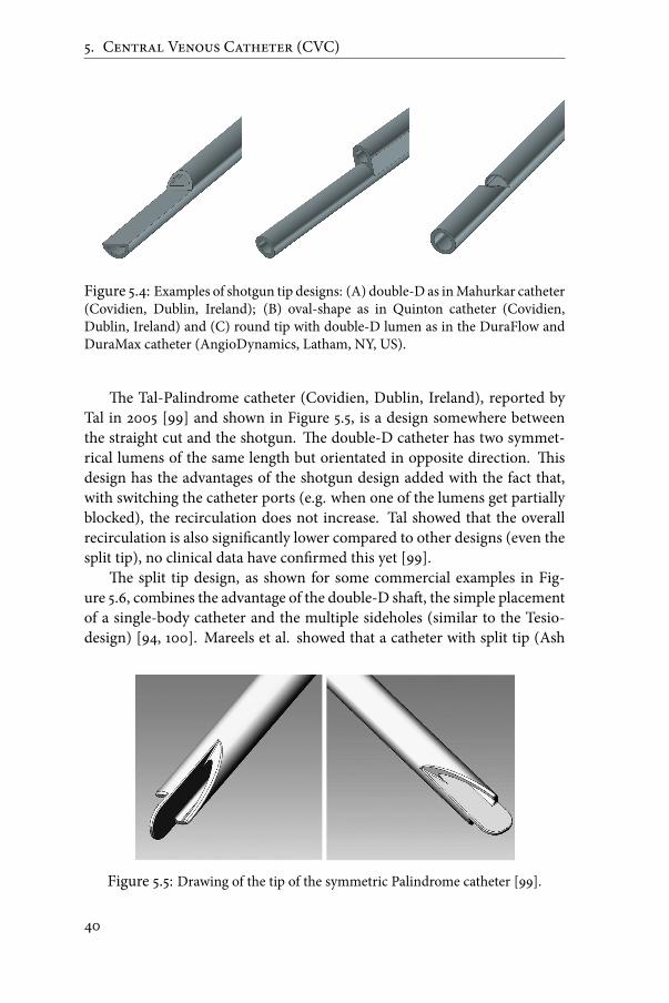
5. Central Venous Catheter (CVC)
Figure 5.4: Examples of shotgun tip designs: (A) double-D as inMahurkar catheter(Covidien, Dublin, Ireland); (B) oval-shape as in Quinton catheter (Covidien,Dublin, Ireland) and (C) round tip with double-D lumen as in the DuraFlow andDuraMax catheter (AngioDynamics, Latham, NY, US).
�e Tal-Palindrome catheter (Covidien, Dublin, Ireland), reported byTal in 2005 [99] and shown in Figure 5.5, is a design somewhere betweenthe straight cut and the shotgun. �e double-D catheter has two symmet-rical lumens of the same length but orientated in opposite direction. �isdesign has the advantages of the shotgun design added with the fact that,with switching the catheter ports (e.g. when one of the lumens get partiallyblocked), the recirculation does not increase. Tal showed that the overallrecirculation is also signi�cantly lower compared to other designs (even thesplit tip), no clinical data have con�rmed this yet [99].
�e split tip design, as shown for some commercial examples in Fig-ure 5.6, combines the advantage of the double-D sha�, the simple placementof a single-body catheter and the multiple sideholes (similar to the Tesio-design) [94, 100]. Mareels et al. showed that a catheter with split tip (Ash
Figure 5.5: Drawing of the tip of the symmetric Palindrome catheter [99].
40

5.3. Devices
Figure 5.6: Examples of split tip designs: �e Ash Split Cath (A) and Split CathIII (B) by Medical Components, Inc. (Medcomp, Harleysville, HA, USA) on thele� and the Pourchez RetrO catheter (C) and HemoSplit XK (D) by C.R. Bard, Inc.(Murray Hill, NJ, USA) on the right.
split) had the lowest arterial tip volume with a shear stress above 10Pa, butthe blood residence time at this location was higher [98].�e Ash Split Cath(Medcomp,Harleysville, HA,USA), launched in 1997, became the ‘gold stan-dard’ catheter for hemodialysis by securing nearly 60% of the U.S. market.To �nalize this overview, the latest variation on the split tip design, the
Centros (Ash Access Technology inc., Lafayette, IN, US) is shown in Fig-ure 5.7.�is self-centering catheter was designed to avoid complete sheath-ing of the catheter and therefore holding a portion of the catheter in themid-dle of the vena cava. �e lumen tips bend inward from the contact pointsat the lumen wall. Side holes are not present because the lumen tips shouldnot be in contact with the vena cava wall and should therefore not becomeoccluded. A seven week study on nine patients showed an increased average�ow for the Centros compared to standard catheters [101].
41

5. Central Venous Catheter (CVC)
Figure 5.7: Centros catheter (Ash Access Technology inc., Lafayette, IN, US) [101].
5.3.4 Catheter-gra� combination
�ere is a combination of a catheter and gra� on themarket under the nameHeRO (Hemodialysis Reliable Out�ow) (Hemosphere, Inc., Eden Prairie,MN, US) as shown in Figure 5.8. �e device has a traditional arterial gra�anastomosis and to avoid the venous anastomosis complications in AVGs(stenosis and thrombosis), the 6mm ePTFE gra� is connected to a 5mm(16Fr.) silicone out�ow catheter. �e venous out�ow component is placedin the central venous vasculature with the distal tip in the right atrium. Aclinical study [102] showed that the infection rate per 1000 catheter days wasreduced to 0.7, i.e. between the values for AVF andAVG.�e device had alsosimilar patency rates compared to AVGs.
Figure 5.8: HeRO gra�-catheter by Hemosphere, inc. (Eden Prairie, MN, US).
42

Chapter
6Comparison between vascular
access options
6.1 Occurrence
�e Dialysis Outcomes and Practice Patterns Study (DOPPS) has shownlarge international variations in vascular access practices.�e patients sur-veyed1 used an arterio-venous �stula in 66% of the cases in Europe, as com-pared to 15% in the United States. A central venous catheter was used in 31%in Europe as compared to 60% in the US. Physicians used an arterio-venousgra� in 2% of the cases in Europe as opposed to 24% in the US [103]. Asmentioned before, elderly, diabetics and female patients tend to have lowerquality native vessels, and therefore a lower patency of AVFs. �is can beseen in the prevalence of AVFs created in the examples shown in Figure 6.1.Allon et al. state, a�er reviewing the literature, that among patients who
are referred for their initial vascular access surgery, placement of a forearm�stula is feasible in only 40 to 50%. However, placement of an upper arm�stula is possible in an additional 25 to 35% of patients. �us, some type of�stula can be placed in at least 75% of patients, with the remainder requiringthe creation of a gra� [30]. So the numbers of �stulas created in Europe arein line with these �ndings, while the large number of AVGs created in theUSshould be decreased. A�er the results of the DOPPS study were published,
1New access types from 1996 until 2000
43

6. Comparison between vascular access options
Figure 6.1: Arterio-venous �stula (AVF) use among patients in Europe (EUR) andtheUnited States (US) for three di�erent patient groups (n refers to the total numberof patients in the particular subgroup) [103].
the Fistula First Breakthrough Initiative (FFBI) was started in July 2003. Atthe start of the DOPPS study, the prevalence rate of AVFs in the US was 24%(80% for Europe)[103] and is now increased to 59.5% (August 2011) [104].However, in recent years, the chronic dialysis population has become
substantially older, more likely to be female and diabetic, and has higher co-morbidity. Many of these patients appear to have vessels of low quality forconstruction of native �stulas. �erefore, it is expected that in Europe thepercentage of AVGs created will increase [21].
6.2 Patency - Mortality
Primary patency is the interval from the time of access placement until the�rst intervention to maintain or re-establish patency or until access throm-bosis. Assisted primary patency is the interval from the time of access place-ment until access thrombosis, in this case including surgical or endovascu-lar interventions to maintain the functionality of a patent access. Secondary(cumulative) patency is the interval from the time of access placement untilaccess abandonment, including surgical or endovascular interventions andeven a�er thrombosis. [105].�is is visualized in Figure 6.2.
�e one year primary patency rates for AVFs and AVGs are similar (43%versus 41%), but when only the matured AVFs are taken into account, thisone year primary patency rate increases to 54% [36, 107].For CVC, patency rates are not frequently described in literature, mainly
due to the short term ormedian-long term (6-9months) use of this vascular
44

6.2. Patency - Mortality
Figure 6.2: Visual explanation of patency rates. Primary patency is theintervention-free access survival. Assisted primary patency is the thrombosis-freeaccess survival. Secondary patency ends when the access is abandoned.[106]
access option. Hodges et al. reported however a primary patency rate at oneyear of 9% [36].When analyzing the secondary patency rates in multiple large studies,
the ratio between one year secondary patency of gra�s versus �stulas is �uc-tuating around 1, as shown in Figure 6.3.Concluding from these secondary patency rates that AVGs are as good
working as AVFs is too easy. When analyzing the revision rate to keep theaccess patent, the interventions required for AVGs is 3 to 4 times highercompared to AVFs (See Figure 6.4). So the costs to keep an AVG from totalfailure will be higher as well as the burden for the patients. For AVGs, it is
Figure 6.3: Secondary patency rate at 1 year for gra�/�stula. Note that the ra-tio is approximately 1.0, indicating comparable secondary patency for gra�s and�stulas.[30]
45

6. Comparison between vascular access options
calculated that for every revision procedure performed, the ‘new’ primarypatency rate is reduced (23-16-17% for revision 1, 2 and 3).For CVCs, when the probability of maintaining the patient on a CVC
(including use of new catheters) is included, the one-year survival is 81%compared to the one-year survival of one single catheter of only 48.7% re-ported byMcLaughlin et al. [108]. While also other values of the cumulativeone-year survival between 47% and 93% were reported in literature [88].
�emortality is two- to three-fold higher in patients who initiate dialysiswith a catheter, as compared to those having a �stula [109]. In numbers, themortality of 16.8% for patients with a non-tunneled CVC and 15.2% for thosewith a tunneled CVC compared to 9.3% and 7.1% for those with an AVGand AVF [110]. Moreover, mortality is reduced by approximately 50% inpatients who switch from a catheter to a permanent access (�stula or gra�),as compared with those who remain catheter dependent [111]. DOPPS dataeven showed that in incident hemodialysis patients, access failure for bothAVG and AVF is greater in patients with prior CVC, even a relative risk of1.81 for AVF failure a�er CVC use is reported [112, 113].
Figure 6.4: Revision rate per access-year for gra�s/�stulas. Note that all of theratios are > 1, indicating a much higher revision rate in gra�s than in �stulas.[30]
46

Two
Engineering tools
47


Chapter
7Global approach (ARCH)
Despite themagnitude of the clinical problem related to AVF-creation, therehas been an absence of novel therapeutic interventions in this �eld due tocomplex mechanisms responsible for AVF complications. Most complica-tions are closely related to both the sudden and sustained hemodynamicchanges involved in AVF creation.With this knowledge, an international consortium submitted a project
to the European Commission (EC) for the FP7-ICT-2007-2 call that gotgranted for 3.5 years starting June 2008 until November 2011.�e project wascalledARCH(Patient-speci�c image-based computationalmodeling for im-provement of short- and long-term outcome of vascular access in patientson hemodialysis therapy 1) and had a working budget of around 3.76millioneuro.�e consortium consisted out of 8 main partners with another 3 ‘thirdparties’ as shown in Table 7.1.
�e ARCH project aimed at the development of a service infrastruc-ture for patient-speci�c assessment, surgical planning and follow-up of thevascular access (Figure 7.1). �is infrastructure was based on a multi-scalecomputational modeling framework, coupling 1D network models of thesystemic circulation to 3D computational �uid dynamics (CFD) or FluidStructure Interaction (FSI) models of selected vascular tracts (stenosed ves-sel segments, branching, anastomosis or venous valves).�e input data was
1http://www.vph-noe.eu/vph-projects
49

7. Global approach (ARCH)
Name Country RoleIstituto di Ricerche Farmacologische ‘Mario Negri’ a Italy EngineeringTechnische Universiteit Eindhoven b The Netherlands EngineeringUniversiteit Gent Belgium EngineeringThe University of Sheffield UK EngineeringMaastricht University Medical Center The Netherlands ClinicalGhent University Hospital b Belgium ClinicalOspedali Riuniti di Bergamo b Italy ClinicalUniversity Medical Centre Ljubljana Slovenia ClinicalPhilips Medical Systems Nederland b.v. The Netherlands IndustryPhilips Electronics Nederland b.v. The Netherlands IndustryEsaote Europe b.v. The Netherlands Industrya Coordinatorb Third party
Table 7.1: Members of the ARCH consortium.
drawn from medical imaging and functional evaluations through innova-tive image analysis and signal processing techniques.�e development andthe validation of the patient-speci�c image-based computational modelingtools were a main feature in the projects outline.
�e general goal was to improve treatment quality and to decrease thecosts ofVA creation andmanagement. A considerable part of the projectwastherefore directly aimed at tackling fourmajor clinical issues in VAmanage-ment: non-maturation, long-term patency, steal syndrome and heart failure.Pilot observational studies were performed on volunteers and on hemodial-ysis patients during model development for calibration and for veri�cationof theoretical predictions.�e consortium published the clinical study pro-tocol for the ARCH project in 2011 [114].
Figure 7.1: ARCH concept: Patient-speci�c modeling for AVF surgical planningbased on medical images [115].
50

Chapter
8General fluid mechanics
8.1 Fluid characteristics
8.1.1 Density
�e mass density or speci�c gravity, ρ, of a �uid is the mass per unit volume(kg/m3). ρ is a function of temperature and pressure. For example, purewater will reach its maximal density at atmospheric pressure at a tempera-ture of 4○C, namely 999.97 kg/m−3. At 37○C and at atmospheric pressure,the density of blood is about 1 050 kg/m3.
8.1.2 Viscosity
Dynamic and kinematic viscosityIf a force acts on a �uid, the �uid will exert a certain resistance to �ow (inter-nal friction).�e rate of resistance is �uid speci�c and is called viscosity. Forexample, syrupwill deform less easily thanwaterwhichmeans that syruphasa higher viscosity than water. �e dynamic viscosity, µ, sometimes simplycalled viscosity, has the dimension of kg/m.s or Pa.s. An old dimension ofµ is poise which equals 0.1 Pa.s. When the dynamic viscosity is negligible(µ ≈0) the �uid is said to be ideal, which means that in this case no shearstress will appear.
�e dynamic viscosity is only slightly dependent on the pressure whileit is highly dependent on the temperature. For �uids, the viscosity will de-crease with increasing temperature as the cohesion and the intramolecularforces will decrease.
51

8. General fluid mechanics
�e viscosity of water, µwater , is 10−3 Pa.s at 20○C and the viscosity ofplasma is around 1.3 10−3 Pa.s at 37○C.�e viscosity of blood is highly de-pendent on the hematocrit level (concentration of RBCs in blood) and willbe discussed in the section on blood rheology (p.54).Another viscosity parameter is the kinematic viscosity, ν. �e relation-
ship between dynamic and kinematic viscosity is:
ν = µρ
(8.1)
in [m2/s] = [kg/(m.s)] / [kg/m3].
Newtonian �uidNewtonian �uids are characterized by a linear relationship between shearstress, τ, and velocity gradient, du/dy, in the x-direction perpendicular tothe �ow direction, also known as Newton’s Law of viscosity (Figure 8.1):
τ = µ dudy
(8.2)
in [N/m2] = [N.s/m2].[1/s]�e velocity gradient, du/dy, is also o�en called the shear rate.
y
u
x0
y=0
dudy(
(
Figure 8.1: Shear stress.
52
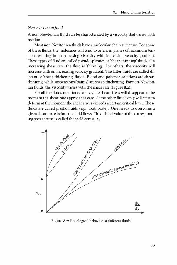
8.1. Fluid characteristics
Non-newtonian �uidA non-Newtonian �uid can be characterized by a viscosity that varies withmotion.Most non-Newtonian �uids have a molecular chain structure. For some
of these �uids, the molecules will tend to orient in planes of maximum ten-sion resulting in a decreasing viscosity with increasing velocity gradient.�ese types of �uid are called pseudo-plastics or ‘shear-thinning’ �uids. Onincreasing shear rate, the �uid is ‘thinning’. For others, the viscosity willincrease with an increasing velocity gradient.�e latter �uids are called di-latant or ‘shear-thickening’ �uids. Blood and polymer-solutions are shear-thinning, while suspensions (paints) are shear-thickening. For non-Newton-ian �uids, the viscosity varies with the shear rate (Figure 8.2).For all the �uids mentioned above, the shear stress will disappear at the
moment the shear rate approaches zero. Some other �uids only will start todeform at the moment the shear stress exceeds a certain critical level.�ose�uids are called plastic �uids (e.g. toothpaste). One needs to overcome agiven shear force before the �uid �ows.�is critical value of the correspond-ing shear stress is called the yield-stress, τ0.
τ
τ0
cass
on-fl
uid
plas
tic
dila
tant (s
hear th
icke
nin
g)
newto
nian
pseudoplastic (shear thinning)
du
dy
Figure 8.2: Rheological behavior of di�erent �uids.
53

8. General fluid mechanics
Blood rheology�e study of the rheological behavior of a �uid implies the hypothesis of acontinuummedium.�erefore, one has to cautiously examine within whichlimits the continuous model is still applicable. It is di�cult to obtain rheo-logical data which is directly related to the whole rheological properties ofblood.�e blood is a complex living medium, which can be considered in a�rst approach as a concentrated dispersion of mainly red blood cells (RBC)(erythrocytes) in blood plasma.If for simplicity a Newtonian model of the blood is used, one should
take into account that the viscosity changes with hematocrit, H. In men theaverage hematocrit is around 45%, in women around 43%, but this value canvary enormously [116]. �e Newtonian viscosity is o�en calculated by theequation derived by Mockros and Leonard for bovine blood[117]:
µ = µp e0.0235H (8.3)
with H the hematocrit (in %) and µp the plasma viscosity. 3.5mPa.s is com-monly used as the Newtonian viscosity value for blood, corresponding to ahematocrit of 42% and a plasma viscosity of 1.3 10−3mPa.s.An example of a shear thinningmodel of blood viscosity is theQuemada
model, depending on the shear rate and hematocrit [118, 119].�e dynamicviscosity is de�ned as:
µ =µp
(1 − 1/2 kH)2 (8.4)
with parameter k a function of the intrinsic viscosities.
k =k0 + k∞
√γ/γc
1 +√
γ/γc(8.5)
with ln k0 = 3.874 - 10.410 H + 13.800 H2 - 6.738 H3ln k∞ = 1.3435 - 2.803 H + 2.711 H2 - 0.6479 H3ln γc = -6.1508 + 27.923 H - 25.600 H2 - 3.697 H3
k0 characterizes the red blood cell aggregation at zero shear stress, k∞describes the orientation and deformation of red blood cells at a shear ratevalue far above the critical shear rate γc and γ characterizes the shear rate.In Figure 8.3, the in�uence of the hematocrit and the shear rate on the
viscosity can be noticed for an example with a plasma viscosity of 1.3mPa.s.For the zones with low shear rate (e.g. bulk �ow in the middle of an arteriallumen), the dynamic viscosity is high (See Figure 8.3, top), while for thezones at the wall (shear rate around 2000), the viscosity decreases to 3.2-4mPa.s (Figure 8.3, bottom).
54

8.2. Fluid dynamics
3.5
4
4.5
5
5.5
6
6.5
20 40 60 80 100 120 140 160 180 200
Shear rate [s ]-1
Dyn
mai
c vi
sco
sity
[m
Pa.
s]
Hematocrit = 35%
Hematocrit = 40%
Hematocrit = 45%
3.2
3.4
3.6
3.8
4
4.2
4.4
200 400 600 800 1000 1200 1400 1600 1800 2000
4.5
Dyn
mai
c vi
sco
sity
[m
Pa.
s]
Hematocrit = 35%
Hematocrit = 40%
Hematocrit = 45%
Shear rate [s ]-1
Figure 8.3: Dynamic viscosity for two ranges of shear rate and three di�erent valuesof hematocrit calculated by the Quemada model.
8.2 Fluid dynamics
Generally, a �uid �ow is a rather complex three-dimensional, time-depend-ent phenomenon. However, in many (biological) situations it is possible tomake simpli�ed assumptions that allow a much easier understanding of theproblemwithout sacri�cingmuch needed accuracy. One of these simpli�ca-tions involves simplifying a real 3D-�ow to a one- or two-dimensional �ow.In almost any �ow situation, the velocity �eld actually contains all three ve-locity components (u, v, w) and each is a function of all three space coordi-nates (x,y,z):
v = uex + vey +wez (8.6)
55

8. General fluid mechanics
In a lot of situations the three-dimensional �ow characteristics are im-portant in terms of the physical e�ects they produce. For these situations itis necessary to analyze the �ow in its complete three-dimensional character.Neglecting one or two of the velocity components in these cases would leadto considerable misrepresentation of the e�ects produced by the actual �ow.�erefore, there are four unknowns, when considering an incompressible,3-D, Newtonian �uid; the three velocity components, u, v and w and thepressure, p.�erefore, there is a need of four independent equations to cal-culate these parameters in every point of the �ow �eld.�ese equations canbe found in the foundational axioms of �uid dynamics also known as thethe conservation laws. �ese conservation laws consist of the conservationof mass, the conservation of momentum and the conservation of energy. Ifonly velocity and pressure are taken into account, the conservation of en-ergy (or �rst law of thermodynamics) can be neglected.�erefore, only theconservation of mass and momentum equations are derived and describedin the following sections.
8.2.1 Conservation of mass
If a di�erential element as presented in Figure 8.4 is considered, the mass�ow in the x-direction is given by:
(ρu + δ(ρu)δx
dx2
) dy dz − (ρu − δ(ρu)δx
dx2
) dy dz (8.7)
Resulting in a net rate of mass out�ow equal to:
δ(ρu)δx
dx dy dz (8.8)
An analysis similar to the one used for the �ow in the x-direction gives theoverall net rate of mass in y-direction and in z-direction, so the net rate ofmass out�ow is given by:
(δ(ρu)δx
+ δ(ρv)δy
+ δ(ρw)δz
) dx dy dz (8.9)
�e rate of mass change in an interval dt is:
(ρ + δρδt
dt) dx dy dzdt
− ρ dx dy dzdt
⇒ δδt
(ρ dx dy dz) (8.10)
�e di�erential equation for conservation of mass is:
δρδt
+ δ(ρu)δx
+ δ(ρv)δy
+ δ(ρw)δz
= 0 (8.11)
56

8.2. Fluid dynamics
X
Z
Y
v
u
dy
dx
dz
w
v+ dy∂v
∂y
u+ dx∂u
∂x
w+ dz∂w
∂z
Figure 8.4: Schematic representation of the velocity in a 3D-di�erential element.
Equation 8.11 is also commonly referred to as the continuity equation. Invector notation, the full conservation of mass equation becomes:
δρδt
+∇ ⋅ ρv = 0 (8.12)
For steady �ow it reduces to:
∇ ⋅ ρv = 0 (8.13)
For incompressible �uids, the �uid density, ρ, is constant throughout the�ow �eld and equation 8.13 becomes:
∇ ⋅ v = 0 (8.14)
orδuδx
+ δvδy
+ δwδz
= 0 (8.15)
In a control-volume approach, the equation is transferred to:
∬c.s.
ρ(v .n)dA+ δδt∭
c.v .
ρdV = 0 (8.16)
With c.s. being the control surface of the control volume, c.v., and n thenormal on the surface.
57

8. General fluid mechanics
8.2.2 Conservation of momentum
Conservation of linear momentum is expressed by Newton’s second law ap-plied to a mass m:
F = m a (8.17)Where F is the resulting force acting on the mass, m, and a the correspond-ing acceleration. In general, two types of forces need to be considered:1. Surface forces, which act on the surface as a result of the interactionwith the surroundings of a �uid element.�ey consist of normal stressdue to pressure and shear stresses due to viscosity.
2. Body forces, which are distributed throughout the �uid element.In analogy with the method used to derive the conservation of mass equa-tion, the resultant surface forces in the x-direction, for a di�erential element,can be seen as:
(δ(σxx)δx
+δ(τyx)
δy+ δ(τzx)
δz) dx dy dz (8.18)
Where σxx represents, as shown in Figure 8.5, the normal stress on a planeperpendicular to the x-direction. τyx and τzx represent the shear stressesin the x-direction on a plane perpendicular to, respectively, the y- and z-direction of the di�erential element.
X
Z
Y
dy
dx
dz
σxx |x+∆x
σxx |x
τyx |y+∆y
τyx |y
τzx |z
τzx |z+∆z
Figure 8.5: Schematic representation of surface forces in the x-direction in a 3D-di�erential element.
For most purposes, the only body force of interest is the weight of thedi�erential element which can be expressed as:
Fx = ρ gx (8.19)58

8.2. Fluid dynamics
Where gx is the component of the acceleration of gravity vector in the xdirection. Other possible body forces are coriolis force or forces due to cap-illarity.When the surface force of Equation 8.18 and the volume force of Equa-
tion 8.19 are inserted in the le� hand side of Equation 8.17, one can derivethe general di�erential equation of motion in �uid in the x-direction:
ρgx +δ(σxx)
δx+
δ(τyx)δy
+ δ(τzx)δz
= ρ (δuδt
+ u δuδx
+ v δuδy
+w δuδz
) (8.20)
Hereby, the right hand side of Equation 8.17 is derived, similar to themethodused in the section on conservation of momentum, by adding the net rate ofmomentum out�ow with the time rate of change of momentum.�e equa-tion can then be simpli�ed by the use of the substantial di�erential DDt , to
ρgx +δ(σxx)
δx+
δ(τyx)δy
+ δ(τzx)δz
= ρDuDt
(8.21)
In contrast to the conservation of mass equation, the conservation of mo-mentumequations should bewritten in all three dimensions, so three equa-tions (x, y and z) make the complete set of equations to solve the conserva-tion of momentum in a �uid. In a control volume approach, these equationsbecome:
∑ F =∬c.s.
ρv(v .n)dA+ δδt∭
c.v .
ρvdV (8.22)
�e three conservation of momentum equations (in all three directions), incombination with the conservation ofmass equation, form together the fournecessary, independent equations to calculate in each point of the �ow �eld(for an incompressible, laminar �ow, with constant viscosity) the unknownsu, v, w and p.
8.2.3 Navier-Stokes equations
�e Navier-Stokes equations are a speci�c representation of the conserva-tion of momentum equations, with inclusion of body force, pressure forceand viscous force.
ρF −∇p + µ∇2v = ρDuDt
(8.23)
59

8. General fluid mechanics
8.2.4 Euler and Bernoulli equations
For the inviscid �ow (ideal �uid) in which all shearing stresses are zero, thegeneral equation of motion is reduced to (in vector notation):
ρg −∇p = ρDuDt
(8.24)
�ese equations are commonly referred to as the Euler equations of mo-tion. It can be seen as a simpli�ed version of the Navier-Stokes equation(with only the gravity taken as body force, F, and with no viscous force in-cluded).If the only external force is the gravity in the z-direction and the equation
is applied to a streamline (1D), the formula reduces to:
z + pρg
+ v2
2g= constant (8.25)
�is is the Bernoulli equation. Note that the equation can only be appliedalong a streamline and that the �ow is assumed to be steady and inviscid. Ifone takes into account the (head) losses, hloss [m], in a �ow from point 1 to2, the Bernoulli equation becomes:
z1 +p1ρg
+ v212g
= z2 +p2ρg
+ v222g
+ hloss (8.26)
An application of this is for instance the blood �ow through a narrow-ing in the coronary arteries (stenosis). When looking at the basic Bernoulliequation (no head losses) for an ‘ideal’ �uid, there will be no pressure gradi-ent over the stenosis, only a transfer in energy (pressure energy pre-stenosisto kinetic energy inside the stenosis and pressure energy recovery post-ste-nosis). A viscous �uid �owing through a narrow stenosis however, intro-duces a signi�cant energy loss. In the contraction segment, the head loss islow when shi�ing the potential energy to kinetic energy. On the contrary, inthe expansion segment, amore ’energy expensive’ transfer is present. Energyis lost by formation and maintenance of vortices (viscous drag) [120].As experimentally shown by Berguer &Hwang (Figure 8.6), in the cases
of a small radius reduction (below 50%of diameter or 75%of area reduction),the �ow is not yet signi�cantly disturbed and the energy recovery, distal tothe narrowed section, is still high (no signi�cant head loss) [120]. When thediameter reduction is above 50% (75% area reduction), the pressure drop hasa quadratic relation with the �ow rate. Here the decrease in blood �ow will
60

8.3. Characteristics of �uid motion
become clinically relevant. If the patient su�ers from a low blood perfusion,for example in his coronary artery due to a stenosis formation, the area re-duction will already be around 75% of the lumen area so that an intervention(e.g. balloon dilation or stenting) becomes necessary.
0 10 20 30 40 50 60 70 80 90 100
flow rate
pressure drop
diameter reduction [%]
area reduction [%]
9590807060504020 3010
Figure 8.6: Qualitative plot of �ow rate and pressure drop over a stenosis based onthe work of Berguer & Hwang [120].
8.3 Characteristics of fluid motion
8.3.1 Laminar and turbulent �ow
�ere is a huge di�erence when a �ow is laminar or turbulent. In laminar�ow, �uid particles move along �xed streamlines with negligible particlemixing across the streamlines. �e �ow is called laminar because it lookslike a series of thin sheets of �uid (laminate) sliding over one another. Aturbulent �ow is characterized by random �uctuations in �uid velocity andby intense mixing of the �uid on macroscopic level and large energy dissi-pation on microscopic level.
�e Reynolds number is used to decide whether the �ow is laminar orturbulent.�e dimensionless Reynolds number is de�ned by :
Re = ρULµ
(8.27)
61

8. General fluid mechanics
where ρ is the �uid density, U the average velocity, L a relevant character-istic length of the studied problem (e.g. the diameter of a vessel) and µ thedynamic viscosity of the �uid.�e Reynolds number is a dimensionless pa-rameter that gives a measure for the ratio of inertial to viscous forces. As arule, one can use for sti� tubes (with L the diameter of the tube):
○ Re < 2000 laminar �ow○ 2000 < Re < 4000 transient �ow○ Re > 4000 turbulent �ow
It should be emphasized, however, that this classical distinction of typesof �ow is only correctly de�ned for steady �ow in rigid tubes. Further-more, complex �ow including the appearance of secondary vortices, doesnot mean that the present �ow �eld is turbulent. By our ‘engineering’-def-inition above, these �ow disturbances might be present in a laminar �owregime. It should be noted that in clinical environments, the term ‘turbulent�ow’ is o�en used for �ow regimes far below the turbulent threshold. Antigaand Steinman stated in their work ‘Rethinking turbulence in blood’ thatblood �ow is typically laminar; however, high frequency �uctuations sug-gesting turbulence have only been observed in vivo in the ascending aortaand arterio-venous gra�s, and in �ows past mechanical heart valves [121].
8.3.2 Poiseuille or plug �ow
When starting from the equation of conservation of momentum, for a hori-zontal tube (no gravity forces), with a stationary, laminar �ow (no derivativeto time) and 1D �ow (v and w are zero) with only a friction and a pressureforce, all applied to a small cylindrical control volume (radius r and lengthL):
(p2 − p1) πr2 = µ δvδr2πrL (8.28)
δvδr
= − r2µL
(p1 − p2) (8.29)
v = − r2
4µL(p1 − p2) + constant (8.30)
For r = R and v = 0 (’no-slip’ at the wall)
v = (p1 − p2)4µL
(R2 − r2) (8.31)
62

8.3. Characteristics of �uid motion
For r = 0, v=vmax (in the center)
vmax =(p1 − p2)4µL
R2 (8.32)
v(r) = vmax(1 − ( rR)2) (8.33)
Note that vavg = vmax/2 and that the velocity is in a quadratic relation to theradius, this is called a parabolic velocity pro�le. An example of the pro�lecan be seen on the le� panel of Figure 8.7 (Section 8.3.3). If we de�ne the�ow rate Q as ∫ R
0 2π v r dr, the expression above becomes:
∆p = 8µLπR4
Q (8.34)
�is is the Poiseuille or Hagen-Poiseuille equation. �is equation statesthat the pressure drop along the tube is directly proportional to the lengthof the tube, the rate of �ow and the viscosity of the �uid, and inversely pro-portional to the fourth power of the internal radius, R.
�is equation is applicable to a steady and laminar �ow in a long andrigid cylindrical tube, with no slip at the wall and a homogeneous and New-tonian �uid.�e term Poiseuille �ow describes this parabolic �ow pro�le.If the �ow pro�le is constant over the radius of the tube, v(r) = vavg =
vmax , it is called plug �ow. When a Newtonian �uid enters a rigid tube witha plug �ow pro�le, a�er a certain length, due to the viscous force, the pro�lewill developed into a Poiseuille �ow pro�le.
8.3.3 Oscillatory �ow
To illustrate oscillatory �ow, we start from the momentum and continuityequations for a homogeneous, incompressible andNewtonian �uid in a rigidcylindrical, horizontal tube (radius R) and assume a periodic motion. �evelocity in the longitudinal direction (x) then becomes:
u = un(r)δpδx
e iωt (8.35)
With (in radial direction)
un(r) =i
ρω
⎡⎢⎢⎢⎢⎣1 −
J0(α rR i3/2)
J0(αi3/2)
⎤⎥⎥⎥⎥⎦(8.36)
63

8. General fluid mechanics
With J0 being a zero order Bessel function and α the Womersley number.�is dimensionless parameter is the square root of a representation of theinertia force divided by the viscous force:
α = R√ω
ν= R
¿ÁÁÀρ.2π f
µ(8.37)
With ω the angular frequency [rad/s] of the oscillations with frequency f[1/s], R the radius of the tube [m] as scale length and ν the kinematic viscos-ity [m2/s].An example of the (scaled) �ow pro�les for di�erent Womersley num-
bers can be found in Figure 8.7. If the Womersley number is small (α<1), aquasi-static Poiseuille pro�le can be found which is in-phase with the pres-sure gradient (as in the Poiseuille equation).�e Womersley pro�les for in-termediate Womersley numbers are characterized by a phase-shi� betweenthe �ow in the boundary layer (near the wall) and the �ow in the centralcore of the tube. If the number is large (α»1), a plug �ow is found which is90 degrees out of phase with the pressure gradient.In a blood vessel network, the frequency, the viscosity and the density
can be assumed to be constant. �erefore the Womersley number is largerin larger vessels and small in smaller vessels. Typical values for a man arearound 22 in the aorta and 4 in the brachial artery.
8.3.4 Shear stress calculations
�e relationship between shear stress,τ, and shear rate, du/dy, as shown inFigure 8.1, is given by Equation 8.2 (Section 8.2). When applying this for-mula in the proximity of the wall, taking the local viscosity and the velocitygradient close to the wall, the Wall Shear Stress (WSS) can be calculated:
WSS = µ ∣δuδy
∣y=0
(8.38)
�is 1D formulation can be transferred to a 3D formulation by taking thederivative of the velocity to the normal, at the wall:
WSSx = µ ∣δuδn
∣wal l
(8.39a)
WSSy = µ ∣ δvδn
∣wal l
(8.39b)
WSSz = µ ∣δwδn
∣wal l
(8.39c)
64

8.3. Characteristics of �uid motion
−1 -0.5 0 0.5 1
0
15
30
45
60
75
90
105
120
135
150
165
180
0
15
30
45
60
75
90
105
120
135
150
165
180
0
15
30
45
60
75
90
105
120
135
150
165
180
0
15
30
45
60
75
90
105
120
135
150
165
180
−1 -0.5 0 0.5 1 −1 -0.5 0 0.5 1 −1 -0.5 0 0.5 1
α = 0.5 α = 4 α = 6 α = 22
Relative radius (r/R) [-]
Ph
ase
an
gle
(ω
.t)
[°]
Figure 8.7: Womersley pro�les for di�erent Womersley parameters assuming aconstant (real) pressure drop over the tube length.�e velocity pro�le is visualizedfor di�erent phase angles [2].
�ese three equations form the wall shear stress vector:
WSS = [WSSx ,WSSy ,WSSz] (8.40)
Time-Averaged Wall Shear Stress (TAWSS)For non-steady �ow regimes, the WSS has a changing value in time. Fora periodic �ow, the Time-Averaged Wall Shear Stress (TAWSS) [Pa] can becalculated as the integral over time of the absolute value of the WSS-vector:
TAWSS = 1T ∫
T
0∣WSS∣dt (8.41)
Malek et al. [122] indicate that in a normal artery the TAWSS should be be-tween 1 and 7 Pa, in a normal vein between 0.1 and 0.6 Pa.�e authors statethat in arterial regionswithTAWSSbelow0.4 Pa, atherosclerosis (arterywallthickening due to the accumulation of fatty substances) will appear, while re-gions with a TAWSS above 7 Pa are only found in narrowed regions such asstenoses or heart valves.
65

8. General fluid mechanics
Oscillatory Shear Index (OSI)To investigate the oscillatory behavior of the WSS, the change in directionof the �ow and therefore the velocity gradient during a cardiac cycle, theOscillatory Shear Index (OSI) [-], originally introduced by Ku et al. [123],can be calculated.
OSI = 12
⎛⎜⎜⎝1 −
∣ 1T ∫T0 WSS dt∣
1T ∫
T0 ∣WSS∣dt
⎞⎟⎟⎠
(8.42)
with
∣∫ T0 WSS dt∣ =
√(∫ T0 WSSx dt)
2+ (∫ T
0 WSSy dt)2+ (∫ T
0 WSSz dt)2(8.43)
For a �ow �eld that highly oscillates, with the numerator (∣∫ T0 WSS dt∣)
equal to zero, the OSI will become 0.5, its maximal value. For a unidi-rectional �ow �eld, over the entire period, the numerator (∣∫ T
0 WSS dt∣)is equal to the denominator (∫ T
0 ∣WSS∣dt) and the OSI becomes zero, itsminimal value.Regions in blood vessels with high OSI indicate a high oscillatory shear
stress on the endothelial cells at the inner wall of the arterial lumen.�is pe-riodic change in direction of the shear stress on the cells, can causes cellularproliferation and intimal hyperplasia growth [41, 55].
Relative Residence Time (RRT)A third wall shear stress parameter that is o�en used, is the Relative Resi-dence Time (RRT) [Pa−1], introduced by Himburg et al. [124] and de�nedas:
RRT = T∣∫ T0 WSS dt∣
(8.44)
�is parameter can also be seen as a weighted combination of TAWSS andOSI:
RRT = 1(1 − 2.OSI).TAWSS
(8.45)
�e parameter is called ‘relative’ residence time, because all particles aremoving and have no absolute residence time on a single location.More hemodynamic wall parameters and their relationship are listed in
the work of Lee et al. [125].
66

8.3. Characteristics of �uid motion
8.3.5 Helicity
Next to parameters evaluating the �ow �eld at the wall, it is possible to char-acterize the �ow in the bulk as well. Belian et al. suggested the use of thedensity of the kinetic helicity per volume unit, Hk .�is parameter seems tohave a great in�uence on the evolution and stability of both turbulent andlaminar �ows [126]. Hk is de�ned as the scalar product of the velocity vector,v and the vorticity vector, ω, of the �ow �eld:
Hk = v ⋅ ω = v ⋅ (∇× v) (8.46)
�e vorticity is the ‘curl’ of the �ow �eld, around an axis (the direction ofthe vorticity vector). For a given total kinetic energy, the kinetic helicity ismaximal when the velocity and the vorticity are in the same direction.�ehelicity is zero, when the direction of the velocity vector and the directionvorticity vector are perpendicular or, of course, when the vorticity or velocityare zero. Grigioni et al. transformed this equation to a Local NormalizedHelicity (LNH) [127, 128]:
LNH = v ⋅ ω∣v∣ ∣ω∣ (8.47)
�e LNH is a parameter between -1 and 1, depending on clockwise or counter-clockwise rotations of the �ow �eld. Finally, the helicity, H, can be de�nedas the volume integral of Hk :
H = 1V∭ HkdV = 1
V∭ v ⋅ (∇× v)dV (8.48)
or of the volume integral of the absolute value of Hk :
H = 1V∭
∣v ⋅ (∇× v)∣ dV (8.49)
�e latter formula is used to avoid that clockwise rotations in the volume canbe compensated by counter-clockwise rotation resulting in a zero volume-averaged helicity. It should be noted that the helicity is function of time,therefore, analysis of the �ow�eld is o�en concluded by calculating the time-average over one cardiac cycle of the helicity.
67


Chapter
9Investigationmethods
9.1 Experimental methods
9.1.1 Particle Image Velocimetry (PIV)
Particle Image Velocimetry (PIV) is a method to visualize the velocity dis-tribution in �uids. As shown in Figure 9.1, a visual clear �uid �ows througha visual clear model, and is seeded with small tracing particle (e.g. 100 µmsilver polyamide particles). �e density of the particles should match thedensity of the used �uid. �e region of interest (ROI) is illuminated with alaser sheet (2D) (e.g. Neodym-YAG (Nd:YAG) laser). A camera records theparticles �owing through the illuminated region of interest (e.g. full frameinterline CCD camera).�e location of the particle over consecutive imagesare compared to achieve the �ow velocity over a de�ned discrete timestep.A 2D velocity �eld can be acquired by use of only one camera to achieve
the velocity in two components (2D-2C standard PIV). If multiple laserplanes, positioned perfectly next to each other, are taken into account, itis possible to calculate even the 3D-2C or even 3D-3C velocity. When stereoPIV is applied, two cameras in an angle of 90 degrees of each other (45 de-grees of the laser sheet) are positioned. Hereby 3 component vectors can becalculated in the 2D plane (2D-3C).Nowadays, the use of PIV for the validation of CFD computations is
a common procedure. In the �eld of biomedical engineering and hemody-namics, many cases have already been published. Next to themore idealized
69

9. Investigation methods
Figure 9.1: General PIV setup [129].
or generalized phantom models of for example an idealized arterial steno-sis [130] or aneurysm [131], PIV validation is applied on a large scale in the�eld of medical devices as central venous catheters [98], blood pumps [132–135], stents [136] or arti�cial heart valves [137–139]. Even when shi�ing toanatomical realistic models, like in studies focusing on the validation of pa-tient speci�c aneurysms [140] or stenosis regions [141], a good agreementbetween in vitromeasurements and computational results was found.Two studieswere performed: (i) a largemulti-center study, inwhich they
compared di�erent PIV algorithms on pre-de�ned models [142], and (ii) aFDA’s ‘Critical Path’ Computational Fluid Dynamics (CFD) / Blood Dam-age Project, in which the use of PIV analysis in the CFD validation processis studied [143]. Both studies concluded that PIV is capable to measure ac-curately the mean (time-averaged) velocities, if the �uctuations in the �owconditions and the �uid properties are minimized.
9.1.2 Experimental assessments on silicon tube models
If a more general assessment of a hydraulic circuit is needed, a siliconmodelcan be constructed.�e siliconmodel does not need to be transparent, as for
70

9.1. Experimental methods
PIV, because it will be used in a hydraulic bench test for pressure and �owevaluations. Once the silicon model is constructed, it can be coupled to astationary or pulsatile pump, with or without adding some �ow splits, wind-kessels or resistances (clamps) before or a�er the model ending. A setup ismostly ended with an open out�ow or with constant height out�ow reser-voirs (Figure 9.2).�e windkessel, when proximal, can be used to adjust thepulse pressure entering the model (damping) or when used distal from themodel to mimic the peripheral compliance.�e height of the out�ow reser-voirs can be set to achieve a constant pressure boundary condition. Out�owdistribution can be changed by opening or closing the clamps.
Figure 9.2: Example of experimental setup consisting of a pump (not shown), awindkessel, connecting tubes, the silicon model, clamps and out�ow reservoirs.Pressure measured by a pressure transducer with pressure-lines and �owmeasuredby a �ow transducer.
To measure the pressure in a model, there are two options. Firstly,needles can be placed in the model, perpendicular to the silicon tube wall.Secondly, �uid-�lled epidural catheters (pressure-lines)(Portex EpiduralCa-theter, Smiths Medical ASD inc., Keene, US) can be slid through the lumenof the model. With the pressure-lines, it is possible to measure the pres-sure on di�erent locations without damaging the lumen. �e needles orpressure-lines are connected to a calibrated �uid-�lled pressure transducer(e.g. P10EZ-1 or DT-X PLUS (Becton Dickinson, Franklin Lakes, NJ, US))which on its turn is connected to a DAQ-unit to process the pressure data.Flow rates can bemeasured by volumetric measurements (collecting the
�uid out�ow for a period of time). Next to this very robust and reliable
71

9. Investigation methods
method, it can be necessary to monitor and analyze the instantaneous �owrate over time.�erefore a �ow transducer (e.g. Transonic �owmeter Team21 Compatible (Transonic Systems Inc., Ithaca, NY, US)) is clamped onto thecircuit.Next to the pressure and �owmeasurements, collecting geometrical data
is important, especially when using the experiment to validate computa-tional results. Most geometrical data can be collected with simple rulers.When for example the diameter at working pressure or the diameter changeduring a pressure change is needed, an ultrasound system (e.g. Picus ul-trasound system, ESAOTE B.V.,�e Netherlands) can be used with, if nec-essary, some wall-tracking so�ware (e.g. ArtLab, ESAOTE B.V.). For ex-act model reconstruction, high resolution X-ray Computed Tomography(micro-CT) can be used with a voxel size down to 210 µm.To have a full set of experimental data, one should determine the �uid
characteristics. Viscosity can be measured with a capillary Ubbelohde vis-cometer (Schott, Germany). Hereby, a U-shaped glass tube is �lled with a�uid and placed in a reservoir with controlled temperature.�e time neededfor the �uid to �ow (by gravity) between 2 prede�ned markers on the cap-illary is taken. �is time can then simply be multiplied by the calibrationfactor of the speci�c glass tube to obtain the kinematic viscosity. �e den-sity of the �uid on the other hand can be measured by �lling a constant vol-ume �ask and comparing its weight with the weight of the �ask �lled withpuri�ed water.Because �uid characteristics might change with temperature (Section
8.1), it is important to monitor the �uid working temperature during theexperiments. When for example a mixture of water-glycerin is used, the vis-cosity can decrease from 8.1 mPa.s to 6.9 mPa.s if the temperature increasesslightly from 18 to 22 ○C (51% glycerin-water mixture).
9.2 Numerical methods
9.2.1 Computational Fluid Dynamics (CFD)
Computational Fluid Dynamics is a computational method to calculate all�uid dynamics (�ow, pressure, heat,...) in a well de�ned domain, with wellde�ned boundary conditions. A �owchart with the di�erent steps in CFDanalysis is shown in Figure 9.3.
�e model is, in the �eld of biomedical engineering, mostly drawn in aCAD program (e.g. SolidWorks (Dassault Systèmes SolidWorks Corpora-
72

9.2. Numerical methods
Model Construction
Meshing
Defining Boundary Conditions
Defining Material Properties
Defining Equations
CFD calculations
Post-processing
CAD: Solidworks
Medical Images: Mimics
VMTK
Gambit
pyFormex
Fluent
Tecplot
ParaView
Matlab
Figure 9.3: Flowchart of Computational Fluid Dynamics analysis with examples ofthe used programs in this work.
tion, Concord, MA, US)) or reconstructed frommedical images (CT-scans)(e.g. Mimics (Materialise, Leuven, Belgium) or vmtk1).Before CFD calculations can start, the �uid domain is split into a dis-
crete number of cells (meshing).�ese volume elements can be either large(coarse mesh) or small (�ne mesh) according to the �uid domain.�e cellscanhave di�erent shapes as tetrahedrons, hexahedrons or prisms.�emesh-ing process can be done in either commercially available packages as Gambit(Ansys Inc., Canonsburg, PA, US) or open-source programs as pyFormex2.Once the domain is meshed, the boundary conditions and material
(�uid) properties should be de�ned. At the wall of the domain (e.g. the ves-sel wall), mostly, a no-slip condition is applied, assuming that the velocityat the wall is zero. At the entrance of the model, a constant or non-constant(e.g. periodic signal (heart rate) �ow rate or velocity can be applied either
1http://www.vmtk.org2http://pyFormex.org/
73

9. Investigation methods
as plug or Poiseuille pro�le (see Section 8.3.2). At the out�ow tracts of thedomain, a �ow distribution can be applied or a pressure or velocity can beimposed. For the used �uid, viscosity and density should be de�ned.Within all cells (�nite volume method), the equations of conservation
of mass and momentum are calculated in relation to the neighboring cells;most o�en, the Navier-Stokes equations (sometimes added with the con-servation of energy) are used (Eq.8.23). For the CFD calculations reportedin this work, the commercial program Fluent (Ansys Inc., Canonsburg, PA,US) was used.If the iterative computations of these equations converge, with low resid-
uals, the �ow and pressure �eld can be analyzed (example in Figure 9.4). Inthis post-processing stage, derivatives of these results, e.g. wall shear stress(See Section 8.3.4) can be calculated. Analysis can either be done directly inFluent, in the post-processing so�ware ParaView (http://www.paraview.org)or Tecplot (Tecplot inc, Bellevue, WA, US) or even in general programs asMatlab (�e Mathworks, Natick, MA, US).
(a) Static pressure
(b) Velocity vectors
Figure 9.4: Arterial (top) and venous (bottom) anastomosis of an AVG con�gura-tion.
74

9.2. Numerical methods
9.2.2 Kinetic modeling
In general, kinetic modeling describes the variation in time of a physicalentity (e.g. mass, energy) which is exchanged among di�erent systems, orbetween a system and the environment.�is dynamic process is ruled by adriving force.
�e human body can be considered as a biological system, consisting ofdi�erent anatomical compartments, which are separated by semi-permeablemembranes. Approximately 58% of the human body consists of water, whichis divided over the extracellular (plasma water and interstitial water) and in-tracellular compartments. Transport between the di�erent compartmentscan happen passively by free di�usion of non-loaded particles (e.g. water,oxygen, urea) or loaded particles (ions), and by forced di�usion via carri-ers or channels. Next to a passive, concentration driven process, transportcan also occur as an active process where the energy is supplied by the ATP(Adenosine TriPhosphate), or as secondary active transport according to anelectrochemical gradient.To describe physiological processes in the human body mathematically,
the body can be divided in di�erent compartments which not necessarilycorrespond to an anatomical reality and in which a physical entity is consid-ered uniformly distributed over the compartmental volume.Such a kinetic model might consist of a large number of arbitrarily small
compartmental entities, necessitating a statistical description.�e resultingformula is then not based on fundamental physical principles, but is derivedfrom (multiple) linear or non-linear regression analyses. However, an im-portant limitation of these statistical models, is that predictions can only besafely made for the parameters that are clinically measured. Instead, inmostcases, a mechanistic model with a limited number of compartments mightbe su�cient to describe solute kinetic behavior.�e advantage of mechanis-tic models is that predictions beyond the scope of the examined parametersare more robust as these models are based on fundamental physical princi-ples such as the conservation of mass and the conservation of energy.So a puremathematical non physiology-basedmodel following the clas-
sic pharmacokinetic approach can be used.�is model may consist of one,two or several compartments/pools (double pool example in Figure 9.5).Each compartment is characterized by a homogenous internal solute con-centration (C1, C2,...) and a distribution volume (V1, V2,...), all changingin time caused by di�erent transport processes: input (I) and output (O)(i.e. de�ned as an interaction in between compartments and/or the envi-ronment), and solute generation (G) and/or elimination (E) (i.e. de�ned astaking place inside the compartment).�e mass input and output might be
75

9. Investigation methods
Volume 1 Volume 2
E1 E2G1 G2
1 1V C
2 2V C
K12
I O
Figure 9.5: General representation of a double pool kinetic model. V: Volume; C:Concentration; G: Generation; E: Elimination; I: Input; O: Output and K12: Inter-compartmental clearance.
proportional to the concentration itself (clearanceK) or to the concentrationdi�erence (intercompartmental clearance K12).Finally, for each compartment separately, themass balance is written as a
di�erential equation. In case ofmore than one compartment, the di�erentialequations should be solved simultaneously and treated as a coupled mathe-matical problem. From the representation in Figure 9.5, the basic equationscan be de�ned as:
d(V1C1)dt
= G1 − E1 + K12 ⋅ (C2 − C1) (9.1a)
d(V2C2)dt
= G2 − E2 + I − O − K12 ⋅ (C2 − C1) (9.1b)
In the �eld of hemodialysis treatment, kinetic modeling can be appliedin two di�erent ways: identi�cation of the unknown model parameters (i.e.calibration of the kinetic model), or simulation of intra and/or interdialyticparameters using an already calibrated kinetic model.Identi�cation is based on the determination of the unknown model pa-
rameters by �tting the solution of the (coupled) mass balance equation(s)to the clinically measured blood or plasma concentrations at di�erent time
76

9.2. Numerical methods
points during dialysis. Problems with identi�cation might arise when toomany parameters are unknown and the measured concentration data setis too small to yield enough accurate information. Calibration has beenperformed previously in the context of hemodialysis for β2-microglobulin(β2M) by Stiller et al. [144], for phosphate by Spalding et al. [145] and forurea and guanidino compounds by Eloot et al. [146].Once a calibrated kineticmodel is available, simulations can be achieved,
predicting the time course of solute concentration for future time points.Hence, simulations allow the comparison of solute removal and/or time-averaged concentrations when applying di�erent dialysis strategies.
77


�ree
Studies on AVFs
79


Chapter
10Computational study of flow in AVF
anastomoses
K. Van Canneyt, T. Pourchez, S. Eloot, C. Guillame, A. Bonnet, P. Segersand P. Verdonck.
Hemodynamic impact of anastomosis size and angle in side-to-endarteriovenous �stulae: a computer analysis.Journal of vascular access. vol.11. 2010:52-58.
81

10. Computational study of flow in AVF anastomoses
10.1 Introduction
�e e�ciency of hemodialysis treatment for end-stage renal disease patientsis to a great extent dependent on the quality of the vascular access. In gen-eral, themost appropriate way of establishing a vascular access is by creatingan arterio-venous �stula (AVF) as �rst described by Brescia et al. in 1966[28] or a modi�cation to this approach. However, as the construction of thisautologous connection between the arterial and venous network is still theunderlying cause of many clinical complications, optimization of the vascu-lar access is the subject of many ongoing and �nished studies as describedby Cimino [29].Nowadays, most clinicians start from the idea of an AVF as a 6 segment
circuit consisting of the proximal artery (1), the distal artery (2), arterial col-laterals (3), the proximal vein (4), the distal vein (5) and venous collaterals(6). However, to have a total hemodynamic description of the AVF, it is im-portant to insert at least a seventh segment in the �ow path, the anastomosisitself.�e 7 segment approach is schematically illustrated in Figure 10.1.
6
1
4
3
2
5
7
Figure 10.1: Seven segment AVF circuit: Proximal artery (1); distal artery (2); ar-terial collaterals (3); proximal vein (4); distal vein (5); venous collaterals (6) andarterio-venous anastomosis (7).
82

10.2. Material and Methods
Given the virtually total absence of studies addressing the geometry ofthe anastomosis in the setting of an AVF, it can be stated that this is an as-pect largely disregarded as a potentially determining factor of the access �ow.�erefore, the present study was set up to study in detail the uncoupled ef-fect of the anastomosis angle and anastomosis size in the setting of arterio-venous �stulas. With Computational Fluid Dynamics (CFD), the pressuredrop and �ow distribution curves were calculated and stream line patternswere studied [147, 148] in order to have an in depth insight in the access �owand the �ow �eld at the anastomosis.
10.2 Material andMethods
A 3-D geometry of a matured side-artery-to-end-vein AVF was designedconsisting of an artery with a diameter of 4 mm connected to a vein witha diameter of 6 mm (Figure 10.2). �e connection was made by an anas-tomosis with given angle (A) and cross-sectional area (CSA), assuming anellipsoidal cross-section with a given anastomosis length (L) and width (W).Steady �ow in the geometry was assumed, following Sivanesan et al. [149].All AVF models were constructed on an in vivo scale in the CAD pack-
age SolidWorks 2005 (SolidWorks Corporation, Concord, MA, U.S.A.) andexported into the grid generation so�ware Gambit 2.2 (Ansys Inc., Canons-burg, PA,U.S.A.) via the IGES (Initial Graphics Exchange Speci�cation) dataformat. �e mass and momentum conservation equations are discretizedand solved in the CFD package Fluent 6.3 (Ansys Inc., Canonsburg, PA,U.S.A.) a�er prescribing all boundary conditions. In the CFD-model, theblood �ow is treated as 3-D, non-pulsatile, laminar, Newtonian (dynamicviscosity of 3.5 mPa.s representing a hematocrit around 40% [116]) and in-compressible [150]. �e post processing of the CFD results was executedusing Tecplot 360 (Tecplot inc., Bellevue, WA, U.S.A.). Regression analy-sis, �tting a quadratic relation to the data, was used to assess the pressuredrop results. Goodness of �t was expressed by the R2 value. Analysis wasdone using SigmaPlot 10.0 (Systat So�ware Inc., San Jose, CA, U.S.A.). Ourstudy addressed two issues: the impact on hemodynamics of the size andthe impact on hemodynamics on the angle of the anastomosis.
10.2.1 Substudy 1: impact of anastomosis size on hemodynamics
�e reference geometry for this �rst substudy, serving as point of compari-son for all results, was an anastomosis characterized by A = 30○, L = 6mmand W = 4mm (CSA = 18.8mm2), with 900ml/min in�ow at the arterialinlet (Qai) and with a �ow distribution of 8% and 92% towards the arte-rial outlet (Qao) and venous outlet (Qvo), respectively (see also Figure 2).
83

10. Computational study of flow in AVF anastomoses
Figure 10.2: Reference arterio-venous �stula con�guration.
�e anastomosis size varied using geometries (LxW) of 8x2, 6x3, 8x3, 6x4and 10x3 (L and W in mm), resulting in a cross-sectional area of 12.6mm2,14.1mm2, 18.8mm2, 18.8mm2 and 23.6mm2, respectively.We �rst calculated the �ow �eld and pressure drop over the anastomo-
sis for 5 di�erent anastomosis geometries, imposing �ve di�erent �ow rates(600, 750, 900, 1050 and 1200ml/min) but maintaining a �xed �ow distri-bution of 8% arterial versus 92% venous out�ow.�e pressure drop over theanastomosis was calculated from the area-averaging static pressure at 25mmfrom the anastomosis in the proximal artery and proximal vein.Second, we ran an additional series of computer simulations to deter-
mine whether the anastomosis size also a�ects the �ow distribution. To doso, the inlet and outlet pressures of the artery (Pai , Pao) and outlet pressure ofthe vein (Pvo) in the reference cases were considered as general conditions.
10.2.2 Substudy 2: impact of anastomosis angle on hemodynamics
Reference for this substudy is an anastomosis characterized by A = 53○, L =6mm and W = 4mm (CSA = 18.8mm2), with 900ml/min in�ow at the ar-terial inlet (Qai) and with a �ow distribution of 8% and 92% towards thearterial (Qao) and venous outlet (Qvo), respectively. �e anastomosis anglewas varied over 27○, 34○, 45○, 53○, 63○, 76○and 90○, a clinically relevant range[149].Again, simulations were �rst done imposing di�erent �ow rates (with a
constant �ow distribution) while studying the pressure drop over the anas-tomosis for the di�erent angles, followed by simulations with �xed pressureboundary conditions and studying the e�ect of the angle on the �ow distri-bution towards arterial and venous outlet.
10.3 Results
10.3.1 Substudy 1: impact of anastomosis size
Figure 10.3a shows the pressure drop over the anastomosis for a �stula �owrange of 600 to 1200ml/min for di�erent anastomosis sizes, but �xed anas-84

10.3. Results
tomosis angle of 30○. As anticipated, the pressure drop decreases with in-creasing anastomosis cross-sectional area. For the smallest anastomosis size(L = 8mm, W = 2mm, CSA = 12.57mm2), the pressure drop varies from8.1mmHg (Qai 600ml/min) to 30mmHg (Qai 1200ml/min), while for thecasewith the largest CSA, (L= 10mm,W=3mm,CSA=23.6mm2) the pres-sured drop starts from 5mmHg (Qai 600ml/min) to rise up to 18.6mmHg(Qai 1200ml/min).�e case of L = 8mm andW= 3mm is almost similar tothe case of L = 6mm and W = 4mm.�is is due to the fact that both caseshave the same cross-sectional area (CSA = 18.8mm2).Figure 10.4a shows the e�ect of anastomosis size on the �ow distribution
for �xed pressure boundary conditions. For increasing anastomosis size, thearterial in�ow increases to �nally stabilize from a CSA of 20mm2 on. Fur-thermore, it is also clear from �gure 4a that �ow distribution is shi�ed to-wards the venous out�owwhen the anastomosis size increases. For a CSA of12.6mm2, the �ow distribution towards the arterial and venous outlet is 22%and 78%, respectively, while these numbers shi� to 5% and 95% for CSA =23.6mm2.
10.3.2 Substudy 2: impact of anastomosis angle
Figure 10.3b shows the pressure drop for di�erent anastomosis angles for a�xed anastomosis size of 6mmx4mm(CSA= 18.9mm2).�e pressure dropslightly increases for increasing anastomosis angle from 26○over 33○to stabi-lize at 45○. For anastomosis angle from 45○up to 90○, the pressure drop de-creases signi�cantly.�e maximal di�erence in pressure drop among casesof di�erent anastomosis angle at 1200ml/min is 12.8mmHg, which is in thesame range as in the parameter study for the anastomosis size of Figure 10.3a(11.4mmHg). Among the studied geometries, the maximal pressure drop isobtained for the 45○anastomosis (24.1mmHg).It can be seen in Figure 10.4b that venous out�ow reaches a minimum
around 43○anastomosis angle, while it is continually increasing for largerangles. Even for an anastomosis angle of 58○, the venous out�ow exceedsthe proximal arterial in�ow, and with it, the �ow in the distal artery changesdirection.
85

10. Computational study of flow in AVF anastomoses
Figure 10.3: (a) Pressure drop over anastomosis versus blood �ow rate for di�erentanastomosis sizes (Length x Width, both in mm), anastomosis angle �xed at 30○.(b) Pressure drop over anastomosis versus blood �ow rate for di�erent anastomosisangles, anastomosis size �xed at 6x4 (CSA = 18.8mm2).
86

10.3. Results
Figure 10.4: (a) Flow rate at arterial inlet, outlet and venous outlet for di�erentanastomosis sizes, starting from reference case L = 6mm; W = 4mm and A = 30○.(b) Flow rate at arterial inlet, outlet and venous outlet for di�erent anastomosisangles, starting from reference case L = 6mm; W = 4mm and A = 53○.
87

10. Computational study of flow in AVF anastomoses
10.4 Discussion
Although several in vitro and computational studies [147, 148] already in-vestigated the �ow in AV-�stulas, none of them focused, according to ourknowledge, on the hemodynamic impact of the geometry of the anastomo-sis. �erefore, the present study was set up to assess the importance of theAVF-anastomosis geometry by calculations of �owdistribution andpressuredrop at the anastomosis site.
�e 6 segment approach (not taking into account the anastomosis) is re-ported in detail in literature overviews, describing AVF-complications andsolutions [151, 152]. When, for example, an ischemic case is presented (whereblood �ow towards the hand is too low because of a too high AVF �ow),suggested solutions are DRIL (distal revascularisation-interval ligation) [47,48], PAI (proximalisation of the arterial in�ow) [49] or RUDI (revision us-ing distal in�ow) [50] to create a longer �ow pathway, besides banding (thenarrowing of the initial draining vein) [51–53] and even creating an arti�cialstenosis in the draining vein [54]. �ose are di�erent solutions, aiming toincrease the AVF �ow resistance, and with it, to decrease access �ow and/orincrease pressure in the distal artery.In this study, we focused on the 7th segment, the anastomosis itself, as
a very important factor in the AVF hemodynamics. In this approach, thereis a clear distinction between the pre- (6 element) and the postoperative (7element) system. Before AVF creation, the main pressure drop between thehigh proximal artery pressure and the low proximal vein pressure is situatedin the distal microcirculation and capillary bed. A�er creation of an AVF asvascular access, the high pressure in the proximal artery ismaintained by thesympathic re�ex which increases the cardiac output and the enlargement ofthe feeding vessels. On the other hand, the low pressure in the proximal veinis maintained by the enlargement of the draining veins. However, the mainpressure drop is now, in the ideal case, situated over the anastomosis. In thiscase, a high arterial pressure and a low venous pressure are maintained.A chronically large anastomosis size causes a small anastomosis resis-
tance.�is small resistance will probably result in a high �ow in the vascu-lar access and the ’main’ pressure drop will now be divided over the anas-tomosis and a narrowing of the vascular system.�is high �ow can triggerischemia. �e model of Barnes et al. enlightened that ischemia is avoidedwhen the ratio of the resistances of the anastomosis versus proximal arteryis smaller than the ratio of the resistances of the distal bed versus the arte-rial collaterals [153]. In the opposite situation, the possibility of �ow reversaland ischemia is signi�cant. Some authors suggest, as ideal solution for these
88

10.4. Discussion
high �ow cases, the closure of the large anastomosis and the creation of ananastomosis with a more appropriate size [153, 154]. But, on the contrary, inin vivo studies where analogous boundary conditions are meant to be cre-ated, anastomosis length (length of surgical incision) variations of 25% arepermitted [155] and the hemodynamic impact of the anastomosis size seemsneglected.�is study shows that this change in anastomosis size has a largeand underestimated impact on blood �ow and local pressures.Beside the size of the anastomosis, a secondparameter determining anas-
tomosis resistance is the angle of the anastomosis, as it will highly determinethe local velocity �eld and hemodynamics, and hence the energy dissipation(pressure drop) over the anastomosis. In literature, the impact of the angleof an anastomosis has been studied in numerical, in vitro and in vivo stud-ies in the domain of distal leg artery bypasses [156], human aorta bypasses[157] and pig aorta bypasses [158], but not in the context of AVF. Althoughthe study of Chua et al. is using the con�guration similar to the side-to-endAVF, the applied geometry has a very small gra�-to-artery diameter ratio of0.3 [157].Because of the lack of studies dealing with the anastomosis resistance,
the present study focused on the anastomosis size and anastomosis angle. Itcan be observed from our results that the pressure drop rises quadraticallywith increasing �ow rate (all curves with R2-values above 0.99) and that,as expected, the pressure drop decreases with increasing anastomosis size.�e quadratic term superimposed on the linear term (as observed inHagen-Poiseuille �ow) in the pressure drop curves is due to the secondary �ow atthe anastomosis site.�is secondary �ow can be seen in Figure 10.5(a-c). Inthe case of 90○, it is clear from Figure 10.5c that at the inner wall, a low �owzone appears.�is can also be seen as a low wall shear stress (WSS) zone inFigure 10.5f, which may lead to a region with increasing intimal hyperplasiaand stenosis formation. Figure 10.5c and 10.5d show aWSS distribution withhigher peak values and less signi�cant low value zone.In the cases exceeding 58○of anastomosis angle, reverse �ow in the distal
artery is present. It should be noted that this ‘steal’, can lead to the distalhypoperfusion syndrome [159, 160] and results in ischemia [44, 161].As limitation of the present study, it can be brought up that the used
geometries and boundary conditions are a simpli�cation of the complexcardio-vascular human anatomy and physiology. For example, the study ofthe cardiac adaptation (with the heart as the eight component of the circuit)was neglected.�e model represents an ideal anastomosis without taking inconsideration parameters as athero- and arterio-sclerosis and intimal hyper-plasia formation, loss of wall distensibility, elasticity of the venous wall, en-dothelial dysfunction, AVF maturation and repeated cannulation,. . .But on
89

10. Computational study of flow in AVF anastomoses
Figure 10.5: Le�: Velocity magnitude [m/s] and in-plane streamlines (sagittalplane); Right: Wall shear stress [Pa] on the wall surface at the anastomosis side.All �gures for in�ow rate of 1200ml/min: (a, d) 27○anastomosis angle; (b, e)45○anastomosis angle and (c, f) 90○anastomosis angle.
the other hand, the idealized model allowed us to study the separated localhemodynamic impact of the anastomosis angle and size, hereby uncouplinganastomosis size and angle from each other and from other anatomic andphysiologic factors. �is is, obviously, di�erent from clinical reality wherethe anastomosis angle and size are not totally independent, but a compro-mise of what is achievable in a given patient with a given arterial and venousterritory.
�e used non-parametric models and relative basic CFD calculationscan be seen as a limitation, but do however not change the overall message90

10.4. Discussion
and conclusion of this study. Numerical values shown in Figures 10.3 and10.3 cannot be seen as absolute values but more as indicative values to showthe global trend of pressure drop and �ow distribution variation in changinganastomosis dimensions. CFD is a well-established technique and it can benoted that the in vitro validation of CFDmodeling has already been done inmany other cases, among others in the �eld of vascular accesses (as in Sec-tion 11.2). Furthermore, it can be remarked that the anastomoses were ovalshaped, due to minimize computational geometric and calculation errors.�e side-artery-to-end-vein con�guration was chosen in this study in favorof the side-to-side alternative, because the choice of anastomosis size andangle is more pertinent in the creation of this AVF [162].Finding an optimal anastomotic length for a �stula, usable for all pa-
tients, is unrealistic due to the varying, patient-speci�c anatomic and phys-iologic conditions. As general idea should it always be kept in mind that themain pressure drop in the arterio-venous circuit should be over the anasto-mosis to avoid high pressure in the venous system and distal ischemia prob-lems. A too small anastomosis on the other hand will have a tendency tonon-maturation or poor �ow during dialysis session.From our clinical practice, the best anastomosis length at the wrist or
forearm is probably 7mm for small vessels. Evolving towards an ellipticshape a�er maturation and therefore taking 3 to 4mm of width, an anas-tomosis size of 16.5 to 22mm2 can be found. �ese sizes are comparablewith the results of lower pressure drop and higher venous out�ow as seenin Figure 3a and 4a. �e angle is, in most cases, easy to make with 30 to45○, depending on the anatomy.�e aim of making an angle of about 135○isdemandingmore vein length andwas therefore also taken out of the compu-tational study. For vessels already dilated, and especially for arteries, with adiameter more than 5mm, the length is best about 5 to 6mm.�ese lengthsgive an anastomosis size between 11.8 to 18.5mm2 (for 3 or 4mm of width),resulting in the higher pressure drop values in Figure 3a. A longer anasto-mosis will cause too much �ow in these cases, from our clinical experience.At the elbow, the reasoningmentioned for dilated, large, arteries can be used.So anastomosis lengths from 5 or 6mmare themost appropriate choice.�eangle to choose is depending on the anatomy, and should vary from 25 to90○. For very big vessels at the elbow, the length ought to be 4mm to avoiddistal ischemia and the evolution toward a very high �ow�stula. Finally, oneshould keep in mind that the initial size of the anastomosis and the vesselsmight change during maturation.
91

10. Computational study of flow in AVF anastomoses
10.5 Conclusion
While the hemodynamic impact of the anastomosis size and angle of anAVFis in many studies and daily practice largely underestimated, we have shownin this computer analysis that the �owdistribution and pressure drop changesigni�cantly with anastomosis size and angle.�e results prove that the AV-anastomosis should be considered as an important and full component ofthe total AVF �ow circuit. In particular, it is shown e.g. that a change of2mm in anastomosis length can increase the pressure drop by more than30%. �erefore, in the surgical creation of an AVF as vascular access, theanastomosis geometry should be chosen with care while keeping in mindthe impact of the geometry on pressure drop and �ow distribution, bothduring creation of a �stula as during complication solving interventions.
92

Chapter
11Experimental validation
W. Huberts1, K. Van Canneyt1, P. Segers, S. Eloot, J.H.M. Tordoir,P. Verdonck, F.N. Van de Vosse and E.M.H. Bosboom.
Experimental validation of a pulse wave propagation model for predictinghemodynamics a�er vascular access surgery.
Journal of Biomechanics. vol.45(9). 2012:1684-1691.
L. Botti1, K. Van Canneyt1, R. Kaminsky, T. Claessens, R.N. Planken,P. Verdonck, A. Remuzzi and L. Antiga.
Validation of a high �ow rate hemodynamics solver on a patient-speci�cmodel of vascular access for hemodialysis.
Submitted.
1Both authors equally contributed.
93

11. Experimental validation
11.1 Experimental validation of pulse wave propagation model
11.1.1 Introduction
Hemodialysis is a common treatment for end-stage renal disease (ESRD) pa-tients [9, 10]. To facilitate hemodialysis, a well-functioning vascular accessis needed. �e vascular access should be able to provide a high blood �owand should be easily accessible for repeated cannulation over time [21, 25].�e preferred vascular access is an arterio-venous �stula (AVF) in the arm,which is a surgically created connection between artery and vein (anasto-mosis), resulting in a signi�cant �ow increase (up to thirtyfold) and vesselremodeling [19, 21, 25, 26].
�e AVF is usually created three months prior to initiation of hemodial-ysis either at wrist level (lower arm AVF) or at elbow level (upper arm AVF)[44, 163–165]. In current clinical practice, the selection is based on the pa-tient’s medical history and the caliber of the involved vessels, i.e. when thecaliber of the radial artery and the distal cephalic vein assessed by duplex ul-trasound exceed 2 mm a lower arm AVF is created, otherwise an upper armAVF. Despite the preoperative diagnostics, complications a�er AVF creationoccur frequently. Lower arm AVFs are hampered by non-maturation in upto 50% of all cases which implies that six weeks a�er surgery, either the AVFis not dilated su�ciently, the blood �ow is too low, and/or the AVF is lo-cated too deep [19, 21, 25, 26, 44, 166]. Upper arm AVFs are hampered bylong-term complications like distal ischemia and/or cardiac failure in 20%of all cases [21, 25, 44, 166].To reduce the number of complications, tools to optimize the location
for an individual patient are therefore of interest. Since a too low brachial�ow directly a�er surgery is associated with non-maturation [26, 167] andsince an immediate postoperative �ow larger than 30% of the cardiac outputis associated with distal ischemia and cardiac failure [44, 163–165], it mightbe bene�cial for surgical decision-making to have a tool that is able to pro-vide, preoperatively, a quantitative patient-speci�c estimate for the immedi-ate postoperative �ow.Previously, a (distributed lumped parameter) pulse wave propagation
modelwas developed that is able to simulate pressure and�owwaveforms af-ter both upper and lower armAVF surgery [168].�is computationalmodel,that is fed by patient-speci�c data was used to predict immediate postoper-ative mean �ows in ten ESRD patients. It was shown that the model selectedthe sameAVF location as an experienced surgeon in nine out of ten patients.However, the postoperative �ow measured by Doppler ultrasound was onlyadequately predicted in six out of ten patients. Di�erences between model
94

11.1. Experimental validation of pulse wave propagation model
predictions and measurements might have several reasons. First, the accu-racy of the measured �ows, input data and boundary conditions might limitthe correspondence between the simulated and measured �ows. Second,the model neglects vascular adaptation and autoregulation of the periph-eral bed which might result in di�erences between measured and predicted�ows. Another reason might be that the physical description of the pulsewave propagation of the pressures and �ows is incomplete.
�e only way to determine if the physical description is complete, is byvalidating the pulse wave propagation model with an experimental setupwhich mimics the surgical AVF procedure and gives the possibility to de-termine a larger number and more accurate mechanical, geometrical andhemodynamic (pressure and �ow waveforms) data than would be possiblein an in vivo situation [169, 170]. In addition, vascular adaptation and regu-lation of the peripheral beds are excluded and do not in�uence the compar-ison of experimental and simulation results. Furthermore, the experimentalsetup can be used to validate the simulated pressure and �ow waveformswhich are needed when adaptation laws will be included in future work.For arteries, in vivo and experimental validation studies for pulse wave
propagation models [169–173] have been performed. However, these studymainly focused on the systemic arterial tree with arterial �owsmuch smallerthan the �ow a�er AVF creation. No validation study is reported that vali-dates a pulse wave propagation model simulating the extreme �ow increasea�er AVF surgery. Moreover, the propagation of measurement uncertaintyin the model input to uncertainty in the model output (i.e. precision) wasnot analyzed previously. However, a quantitative estimate of the precision isrequired for a proper comparison as well as when inferences based onmodelpredictions will be made.�e output uncertainty can be assessed by using amethod based on generalized chaos expansion [174] or by means of MonteCarlo simulations [175]. �e advantage of the method of Xiu et al. is thatless model runs are needed than for Monte Carlo simulations. However, theimplementation is less straightforward since the model equations are madestochastic and the most suitable polynomials for expansion of the stochasticfunction need to be selected.
�e aim of this study is to validate the previously developed distributedlumped parameter pulse wave propagationmodel for the prediction of pres-sure and �ow before and a�er AVF creation. In this way it is determined ifthe physical description of the pulse wave propagation is correctly capturedby the model. �e uncertainty in pressure and �ow waveforms, resultingfrom uncertainties in the model input parameters, is accounted for by usingMonte Carlo simulations.
95

11. Experimental validation
�e manuscript is outlined as follows. First, the experimental setup isdescribed and how mechanical, geometrical and hemodynamic propertiesare determined. �is is followed by a brief description of the distributedlumped parameter pulse wave propagation model. Next, it is discussed howthe model was adapted to the experimental conditions and how the modelwas validated with the experimental setup. In this context, the uncertaintyanalysis is described in detail.
11.1.2 Material and methods
In vitro experimental setupPrevious studies that used an experimental setup consisting of silicone tubesto validate a pulse wave propagation model mainly focused on the systemicarterial tree [170, 173] or single arterial tubes [172]. In addition, the simu-lated arterial �ows were much smaller than the �ows in the arm a�er AVFcreation. In this study, a pulse wave propagationmodel is validated that sim-ulates the �ow increase a�er AVF surgery. Furthermore, the hemodynami-cal complex anastomosis is incorporated in this experimental study, whereasthis was not addressed earlier in a silicone tube network.
�e experimental silicone tubemodel,mimicking the anatomy andphys-iology of the human vasculature in the arm, was built based on patient-speci�c data obtained in a previous study [168]. �e arterial geometricaldata, obtained from magnetic resonance (MR) and ultrasound (US) exami-nations, were used to generate a three-dimensional (3D) CAD-model whichwas used as benchmark for manufacturing the 3D silicone tube model. Forthe construction of the silicone arterial model, Rapid Prototype models anddip-coating techniqueswere used (in-house techniques and knowledge).�evenous silicone model, representing the venous out�ow tract, was based ongeometrical data obtained from US measurements of an ESRD patient andwas constructed by painting silicone, layer by layer, on a steel rod [176].�istechnique was chosen over dip-coating techniques as it was expected to re-sult in lower wall thicknesses and thus lower sti�ness. To mimic the AVF,the arterial and venous silicone models were connected by an anastomosiswith an aperture of approximately 15mm2 and an in-plane angle of 30○ [34].�e resulting silicone network model consisted of the brachial, radial, ulnarand interosseus artery (arterial tract) and of the cephalic, basilic, axillaryand subclavian vein (venous tract).
�is network model was built in a mock loop [177, 178] including a sili-cone aorta and subclavian artery constructed by Hemolab B.V. (Eindhoven,�e Netherlands)(Figure 11.1, top). �e arterial and venous silicone net-work was placed in a water tank to allow for ultrasound measurements.
96

11.1. Experimental validation of pulse wave propagation model
12 3
4
5
6
7
8 10
14
11
13
15
19
16
17 18
9
12
Experimental setup
Computational domain
Water reservoir
Aorta
Pump
Windkessel
brachial
radial
ulnarintero
s.
aorta
subcl.a.
cephaliclower armcephalicupper arm
basilic
subcl.v.
m.cubital
Figure 11.1: Network model mock loop scheme (top) and computational domain(bottom).�e numbers refer to the edges given in Table 11.2. Pressure (x) and �ow(0) waveform acquisition locations are shown.
�e complete circulation circuit was �lled with water and the water waspumped through the mock loop by a step pump (Parker Hanni�n GmbH,O�enburg, Germany) that was regulated by a normalized modi�ed sinus-squared ISO5840 function (Figure 11.2) in LabView (National InstrumentsInc., Austin, Texas, USA).�is resulted in a pump �ow rate of approximately5 l/min which is comparable to a physiological cardiac output [179]. �e�uid entered the proximal aorta via a �exible valve (Hemolab B.V) and couldtherea�er �ow in two directions: to the distal aorta which was closed by awindkessel, and to the subclavian artery which was the in�ow artery of the
97

11. Experimental validation
0 10
1
Time [s]
No
rma
lize
d a
mp
litu
de
[−
]
Figure 11.2: Pump input step function (modi�ed sinus-squared ISO5840).
silicone network model.�is silicone network model had three out�ows inthe arterial part (at radial, ulnar and interosseus artery) and one in the ve-nous part (at the subclavian vein). Formimicking the preoperative situation,the venous out�ow was closed with a clamp, whereas for the postoperativesituation the clamp was released to mimic the presence of a lower arm AVF.�e lower arm AVF was chosen because it involves the largest arterial andvenous network and thus the most complex topology was studied.
Experimental measurement techniquesGeometrical measurements. �e lengths of all arteries, connecting tubesand veins weremeasured using a ruler. In addition, the ruler was used to de-termine the location of the anastomosis with respect to the brachial bifurca-tion.�e proximal and distal arterial and venous diameters were measuredat working pressure with ultrasound (Picus ultrasound system, ESAOTEB.V.,�e Netherlands).�e diameters of connecting tubes were determinedwith a micrometer.
Flowmeasurements. Flowwaveformsweremeasured, at the proximal aortaand the proximal subclavian artery (Figure 11.1) with a Transonic �ow me-ter acquisition system (Team 21 Compatible, Transonic Systems Inc., Ithaca,NY,USA).�e signal was sampled at 500Hz using a data-acquisition (DAQ)unit (BMC-2090, National Instruments Inc.).�e acquisition so�ware wasprogrammed in LabView (National Instruments Inc., version 7.1, Austin,Texas, USA). For all out�ow tracts, the time-averaged out�ows were mea-sured volumetrically.
98

11.1. Experimental validation of pulse wave propagation model
Pressure measurements. Pressure waveforms were measured, using pres-sure transducers (P10EZ-1, Becton Dickinson Critical Care Systems, Sin-gapore) connected to a multi channel compact ampli�er system (PICAS,Peekel Instruments, Rotterdam,�e Netherlands).�e measurements wereperformed at prede�ned locations along the experimentalmodel (Figure 11.1)by sliding a �uid-�lled epidural catheter (Portex Epidural Catheter, SmithsMedical ASD inc., Keene, USA) through the experimental model.�e pres-sure transducers were also connected to the DAQ-unit.
Mechanical properties of the silicone vessels. �e diameter change (dis-tension) of the arteries and veins was measured by using wall-tracking so�-ware (Artlab) that is incorporated in the Picus ultrasound system (ESAOTEB.V.,�e Netherlands). Since pressures were measured simultaneously, thedistension, ∆d, and the pulse pressure, ∆p, were used to determine the localdistensibility, D:
D = 1A0
∂A∂p
≈ 1A0∆A∆p
= 2ddia∆d + (∆d)2d02∆p
(11.1)
in which A0 and d0 are the cross-sectional area and the diameter at meanpressure, and ddia the diastolic diameter.�e distensibility of the subclavianartery was estimated by using its wall-thickness-to-radius ratio of 0.1 and byassuming the Young’s modulus equal to the one of the experimental aorta,as the subclavian artery was made from the same material.�e distensibili-ties of the connecting tubes were assessed from static volumetric compliancemeasurements or set to 10−7 Pa−1 otherwise.
Pressure dropover the anastomosis.�e extra pressure drop over the anas-tomosis was captured via a minor loss coe�cient, de�ned as Kloss = ∆p
12 ρv2 ,
in which ∆p is the pressure drop from the in�ow artery to the out�ow vein,ρ is the density, and v is the mean blood velocity in the in�ow artery. Klosswas determined bymeasuring the pressure drop as function of the Reynoldsnumbers from Re=200 to 3500 (Figure 11.3A).
Mathematical model�e pulse wave propagation model used here was previously developed byHuberts et al. [168], and will only be described in short.�e computationaldomain for the simulations consisted of a truncated part of the aorta, thesubclavian, brachial, radial, ulnar and interosseus arteries, the anastomosis,the cephalic, median cubital, basilic, axillary and subclavian veins, and, in
99

11. Experimental validation
0 1000 2000 3000 4000 50000
10
20
30
40
50
60
70
80
90
100
Reynolds number [−]
Klo
ss [
−]
A
Experimental
Trendline
0 5 10 15 200
10
20
30
40
50
60
70
80
90
100
Anastomosis Angle [°]
Kv [
−]
B
0 1000 2000 3000 4000 50000
3
6
9
12
15
Reynolds number [−]
An
ast
om
osi
s A
ng
le
[°]
C
Klo ss = 1000 · Re − 0.53K v = k2cot
2θ
Figure 11.3: �e experimentally derived minor loss coe�cient as function of theReynolds number (A) and the reducedminor loss equation (Equation (11.4)) imple-mented in thewave propagationmodel developed byHuberts et al. [168] as functionof anastomosis angle (B). In panel C, the comparison between the experimentallyderived loss coe�cient (Reynolds number) and the loss coe�cient implemented inthe wave propagation model (anastomosis angle) is shown.
addition, all connecting tubes (Figure 11.1, bottom).�e vessels were dividedin segments with a maximum length of 5 cm. In each segment the local rela-tion between pressure and �ow is described. For the scope of modeling thee�ect of vascular access creation on blood pressure and �ow distribution,segments are needed that represent arteries, veins and the anastomosis. Allarterial and venous segments weremodeledwith a lumped parametermodelderived from local mass and momentum equations. �e anastomosis seg-ment was modeled with a nonlinear resistance based on two semi-empiricalloss coe�cients, Kv and Kd , that describe the loss from the proximal arteryto, respectively, the proximal vein and the distal artery and have been de-�ned by Gardel [180, 181]:
Kv = k1(1 − q∗)2 + q∗2[k2cot θ2 − k3 + k4−k5A∗
A∗2 ] + k6q∗(1 − q∗)(1 + 1A∗ )cot
θ2 (11.2)
Kd = k7(1 − q∗)2 + k8q∗2 − k9q∗(1 − q∗) (11.3)
in which q∗ is the ratio between �ow through the vein and �ow throughthe proximal artery, A∗ is the ratio between cross-sectional area of the veinand cross-sectional area of the proximal artery and θ is the angle betweenproximal artery and proximal vein. Empirically determined values for theconstants k1 to k9 are given in Table 11.1.
100

11.1. Experimental validation of pulse wave propagation model
k1 k2 k3 k4 k5 k6 k7 k8 k90.95 1.3 0.3 0.4 0.1 0.4 0.03 0.35 0.2
Table 11.1: Semi-empirical determined dimensionless constants k1 to k9 for equa-tion (11.2) and (11.3).
Parts of the cardiovascular system, for which no detailed information onpressure and �ow was required, were truncated and terminated with three-element windkessel models. Assembling all lumped segments resulted in asystem of di�erential equations that describes the pulse wave propagationof the pressure and �ow waveforms. �is system was solved by numericalintegration applying the trapezium rule for implicit time integration. Onthe �rst node, a measured (aortic) �ow was prescribed, whereas the venousout�ow was closed with a �xed intravenous pressure.In this study, pressure and �ow waveforms of the pulse wave propaga-
tion model were validated with experimentally derived pressure and �owwaveforms.�e input parameters of the pulse wave propagationmodel wereadapted to the experimental setup. For this, geometrical (vessel length, ves-sel diameters) and mechanical characteristics of the vessels (vascular com-pliance) were mandatory. Furthermore, information on anastomosis con-�guration (location, angle), windkessel parameters, �uid properties (den-sity and dynamic viscosity), intravenous pressure and an input (aortic) �owwaveformwere required. How these input parameters were obtained will bediscussed in the next section.
Experimental validation: Model parameters for the pulse wave propagationmodel�e input parameters for the pulse wave propagation model were derivedfrom the measurements and are given in Table 11.2. In addition, uncertaintydomains of these input parameters were estimated as they are input for theuncertainty analysis.
Geometrical parameters. �e measured lengths were directly used in thepulse wave propagation model and the uncertainty domain was set to ± 5%,which equals to ameasurement error of 1 mm in the shortest vessel. Also theposition of the anastomosis was variedwithin± 5%.�e uncertainty domainfor the diameters was set to ± 10%. For the arterial and venous diameters,linear tapering within a vessel was assumed. �e in�uence of tapering wasinvestigated by changing the smallest diameter of a vessel while changing
101

11. Experimental validation
the largest diameter in the opposite direction. �e uncertainty domain forthese changes were based on 10% of the smallest diameter.
Mechanical parameters. For the pulse wave propagation model, the localvessel wall compliance per segment length was needed.�is was derived bymultiplying the distensibility in Table 11.2 by the local cross-sectional area,thus assuming a constant distensibility within each vessel. For the distensi-bilities obtained with ultrasound, themeasurement uncertainty domain was± 15%, whereas for the distensibilities derived by volume compliance mea-surements, the measurement uncertainty domain was ± 20%.
Pressure drop over the anastomosis. To match the minor loss coe�cientsin the pulse wave propagation model with the measured loss coe�cient, weassumed that the majority of the proximal artery �ow �ows through theproximal vein (q∗ ≈ 1) and that the arterial and venous cross-sectional areaswere almost similar (A∗ ≈ 1). Equation 11.2 and Equation 11.3 then reduce to
Kv = k2cotθ2− k3 + k4 − k5 = 1.3cot
θ2and Kd = 0.35 (11.4)
�is relationship for Kv is shown in Figure 11.3B. For an anastomosis angle,θ, between 3 and 12 degrees, the loss coe�cient, Kv , matches the experi-mentally determined loss coe�cient, Kloss, in the range of Reynolds num-bers 250-4000 (Figure 11.3C). Finally, the loss coe�cient, Kv , was modeledby the original Equation 11.2, while the anastomosis angle was varied be-tween 3 and 12 degrees. Because the �ow through the distal artery was smallcompared to the �ow through the proximal vein, loss coe�cient, Kd , wasneglected.
Constants. �e �uid used in the experiment was water which has, at roomtemperature (20○C), a density of 103 kg/m3 and a dynamic viscosity of 10−3Pa.s.�ese model parameters would hardly vary during the experiment andtherefore the uncertainty domains were set to ± 1% and ± 5%, respectively.
Boundary conditions. �e peripheral resistance, Rp, of each windkesselwas determined as the ratio of local mean pressure and local mean �ow.�elocal mean �ow was assessed by the volumetric measurements, while themean pressure was assessed by time-averaging the measured local pressurewaveforms.�e characteristic impedance, Z0, was assessed by using
√ρ
DA02
in which ρ is the blood density, D the local distensibility and A0 the cross-sectional area [182].
102

11.1. Experimental validation of pulse wave propagation model
Finally, the compliance, C, for each windkessel was determined by di-viding the time constant, by the di�erence between the peripheral resistanceand the characteristic impedance (Rp−Z0). For the aorta, the time constantwas assessed from the local pressure waveform via the ‘area method’ [183].�e time constant in the radial artery was assessed frommultiplying the lo-cal peripheral resistance with the compliance of the out�ow tube. For theulnar and interosseus arteries, the radial artery time constant was assumed.As a result, the time constant was 5.4 s in the aorta and 0.4 s in the otherout�ow arteries. In the uncertainty analysis, the time constants were variedby ± 20%.For the in�ow boundary at the aorta (i.e. the ascending aorta �ow),
we used the pre- and postoperative aortic �ow measurements, with an esti-mated uncertainty domain of ± 5%. As out�ow condition at the subclavianvein, we used the measured mean pressure with an uncertainty domain of± 10%.
Uncertainty analysisSimulations with the pulse wave propagation model were performed forboth the pre- and postoperative con�guration. To examine the propaga-tion of input uncertainty to the output, Monte Carlo simulations were per-formed. Varying all input parameters independently within their uncer-tainty domain might result in non-physiological combinations of input pa-rameters and thus non-physiological output (e.g. a small artery continuingin a larger artery).�erefore, the input parameters of adjacent vessels werechanged simultaneously (Table 11.2). �is resulted in 44 independent in-put parameters for the preoperative con�guration and 58 parameters for thepostoperative con�guration. Input samples were generated by Latin Hyper-cube sampling, i.e.: For each input variable, its previously de�ned uncer-tainty domain is divided into equiprobable intervals and within each inter-val a value is randomly selected. Consequently, an input value is used onlyonce for each interval and a full coverage of the parameter input space is ob-tained [184]. One sample is thus a point in the input parameter space. �etotal number of samples generated was 5000 times the total number of inputparameters in analogy with previous studies of Huberts et al. [185].For the preoperative con�guration, the simulated pressure waveforms
in the aorta, the proximal and distal brachial artery, the proximal and distalradial artery and the proximal ulnar artery were compared to the measuredpressure waveforms (Figure 11.1, bottom). �is was extended by the distaland proximal cephalic vein, and the basilic vein for the postoperative con-�guration. �e �ow waveforms were compared at proximal aorta and sub-clavian artery. For the comparisons, the median of the simulated pressure
103

11.Experim
entalvalidation
Edge name Edgenumber Length [mm] Diameter [mm] Distensibility [Pa−1] Mean flow [ml/min] Mean pressure [mmHg] Time con-
stant [s]begin end pre post pre post
rigid connecting element 1 50 (5%) 28.9 (10%) 28.9 (10%) 10−7 a(-)proximal aorta 2 150 (5%) 28.9 (10%) 28.9 (10%) 2.1 ⋅10−5 (15%)distal aorta 3 310 (5%) 28.9 (10%) 28.9 (10%) 2.1 ⋅10−5 (15%) 4650 (10%) 4375 (10%) 98 (10%) 90 (10%) 5.4 (20%)subclavian artery 4 100 (5%) 8.0 (10%) 8.0 (10%) 7.7 ⋅10−6 b(20%)rigid (tapered) connectingtube 5 60 (5%) 8.0 (10%) 10 (10%) 10−7 a(-)
compliant connectingtube 6 130 (5%) 10 (10%) 10 (10%) 1.1 ⋅10−6 b(20%)
rigid connecting tube 7 80 (5%) 10 (10%) 10 (10%) 10−7 a(-)compliant (tapered) con-necting tube 8 20 (5%) 10 (10%) 6.0 (10%) 1.1 ⋅10−6 b(20%)
rigid connecting tube 9 55 (5%) 6.0 (10%) 6.0 (10%) 10−7 a(-)brachial artery 10 215 (5%) 6.0 (10%) 4.5 (10%) 1.7 ⋅10−5 (15%)proximal ulnar artery 11 67 (5%) 3.6 (10%) 3.6 (10%) 1.1 ⋅10−5 (15%)distal ulnar artery 12 173 (5%) 2.7 (10%) 1.9 (10%) 1.7 ⋅10−5 (15%) 46 (10%) 42 (10%) 96 (10%) 88 (10%) 0.4 (20%)interosseus artery 13 110 (5%) 1.3 (10%) 1.3 (10%) 1.1 ⋅10−5 (15%) 5 (10%) 5 (10%) 98 (10%) 88 (10%) 0.4 (20%)radial artery 14 240 (5%) 3.4 (10%) 3.2 (10%) 1.5 ⋅10−5 (15%) 50 (10%) 46 (10%) 96 (10%) 84 (10%) 0.4 (20%)cephalic vein lower arm 15 210 (5%) 2.9 (10%) 3.0 (10%) 1.4 ⋅10−5 (15%)cephalic vein upper arm 16 180 (5%) 4.3 (10%) 4.3 (10%) 2.4 ⋅10−5 (15%)subclavian vein 17 32 (5%) 5.6 (10%) 5.6 (10%) 8.4 ⋅ 10−6 (15%) 5.7 (10%) 5.7 (10%)median cubital vein 18 30 (5%) 4.5 (10%) 4.5 (10%) 8.4 ⋅10−6 (15%)basilic vein 19 180 (5%) 4.5 (10%) 4.6 (10%) 8.4 ⋅10−6 (15%)a Assumed value for the rigid tubes.b Estimated from static volume compliance measurements.
Table 11.2: All input data for the wave propagation model that are derived from measurements on the experimental setup. �e meanpressure, mean �ow and time constant are only given for the edges that are closed by a windkessel segment. In brackets the estimatedmeasurement uncertainty is given in percentages.�e vessels that are changed simultaneously during the uncertainty analysis are groupedin one cell.
104

11.1. Experimental validation of pulse wave propagation model
and �ow waveforms of all Monte Carlo simulations was used as well as acon�dence interval, formed by the 25th and 75th percentile interval.
11.1.3 Results
Preoperative resultsTable 11.3 shows that the simulated mean �ows correspond to the measuredmean �ows in the aorta, subclavian artery, the radial artery and the ulnarartery. �e shapes of the simulated aorta and subclavian artery �ow wave-forms correspond to the measured �ow waveforms, though the simulatedsubclavian artery �ow appears less attenuated (Figure 11.4).For all arteries, simulated andmeasuredmean pressures are similar (Ta-
ble 11.3).�e shapes of the simulated pressure waveforms (Figure 11.4) cor-respond to the measured pressure waveforms, although the simulated pres-sures are less attenuated resulting in amore pronounced second peak, whichis clearer in distal pressure waveforms. For the aortic pressure waveform, aphase di�erence of approximately 50ms is observed. Presumably, the tim-ing of the measured aortic pressure waveform is inaccurate as the systolicpressure peak arrives before the �ow peak.
Mean pressure [mmHg] Mean flow [ml/min]measureda simulatedb measureda simulatedb
proximal aorta 95 93 (88,99) 4750 4747 (4682,4813)subclavian artery 101 98 (36,161)proximal brachial artery 98 93 (88,99)distal brachial artery 98 93 (87,99)proximal ulnar artery 98 93 (87,99) 46 44 (35,53)proximal radial artery 98 93 (87,99) 50 48 (34,63)distal radial artery 98 92 (86,99)aMeasured value without uncertainty interval.bMedian value with 25th and 75th percentiles.
Table 11.3: Measured preoperative mean pressures and �ows and their simulatedvalues.
Postoperative resultsDuring the analysis of the postoperative results it was observed that, in �rstinstance, the resistance in the distal cephalic vein was not properly deter-mined. A�er excising the distal cephalic vein from the setup, a non-smoothvessel lumen that was twisted over the full length was found resulting in alarge pressure drop of 24mmHg from the distal cephalic vein to the proximalcephalic vein (Table 11.4). �is pressure drop was approximately ten timeslarger than the expected pressure drop as calculated from Poiseuille’s law.As this additional pressure drop was not captured by the model, all Monte
105

11. Experimental validation
Median of simulation results
25th-75th percentile of
simulation results
Experimental result
60
80
100
120
140
160
0 1Time [s]
Pre
ssu
re [
mm
Hg
]
0 1Time [s]
Pre
ssu
re [
mm
Hg
]
70
90
110
130
150
40
60
80
100
120
140
160
0 1Time [s]
Pre
ssu
re [
mm
Hg
]
60
80
100
120
140
160
0 1Time [s]
Pre
ssu
re [
mm
Hg
]
0 1−1
0
1
2
3
4x 10
4
Time [s]
Flo
w [
ml/
min
]
Proximal aorta
70
80
90
100
110
120
130
140
0 1Time [s]
Pre
ssu
re [
mm
Hg
] Proximal aorta
0 1
−500
0
500
1000
1500
Time [s]
Flo
w [
ml/
min
]
Subclavain artery
40
60
80
100
120
140
160
180
0 1Time [s]
Pre
ssu
re [
mm
Hg
] Distal radial artery
Proximal brachial artery
Distal brachial artery
Proximal ulnar artery
Proximal radial artery
-1000
Preoperative
Arteries
Figure 11.4: �e preoperative pressure and �ow waveforms on several arterial lo-cations.
Carlo simulations were performed oncemore with a tenfold increased resis-tance in the distal cephalic vein with an uncertainty of ± 10%. Since vesselabnormalities could also be present in human vasculature and the resultingadditional pressure drop has signi�cant e�ect, the results of both analyses,with and without the extra resistance, are presented in Table 11.4.When considering the additional resistance of the distal cephalic vein,
the simulatedmean �ow of the subclavian artery and the distal cephalic veinin Table 11.4 now correspond to the measured mean �ow. Beside a betteragreement between measured and simulated �ows, this is also the case forthe pressures. In Table 11.4, it can be observed that the previous observedunderestimation of the measured mean arterial �ows and pressures are re-duced, while measurements and simulations now coincide. �is especially
106

11.1. Experimental validation of pulse wave propagation model
holds for the distal cephalic vein pressure. As in the preoperative simula-tions, the simulated arterial pressure waveforms (Figure 11.5) are less atten-uated than the experimentally measured ones. In addition, a similar phasedi�erence in the aorta is observed.�e shape of themeasured and simulatedvenous pressurewaveforms (Figure 11.6) are similar, although the di�erencesare larger than for the arterial site, i.e. a phase di�erence of approximately50ms in the proximal cephalic and basilic vein.
Median of simulation results
25th-75th percentile of
simulation results
Experimental result
0 1Time [s]
Pre
ssu
re [
mm
Hg
]
0 1Time [s]
Pre
ssu
re [
mm
Hg
]
0 1Time [s]
Pre
ssu
re [
mm
Hg
]
0 1Time [s]
Pre
ssu
re [
mm
Hg
]
0 1−1
0
1
2
3
4x 10
4
Time [s]
Flo
w [
ml/
min
]
Proximal aorta
Pre
ssu
re [
mm
Hg
]
0 1Time [s]
Flo
w [
ml/
min
]
Subclavain artery
0 1Time [s]
Pre
ssu
re [
mm
Hg
] Distal radial artery
Proximal brachial artery
Distal brachial artery
Proximal ulnar artery
Proximal radial artery
Postoperative
60
80
100
120
140
−500
0
500
1000
1500
20
40
60
80
100
120
140
160
Proximal aorta
600 1Time [s]
70
80
90
100
110
120
130
140
50
100
150
75
125
50
100
150
75
125
50
100
150
75
125
Arteries
Figure 11.5:�e postoperative pressure and �ow waveforms on several arterial lo-cations for simulations with additional resistance.
11.1.4 Discussion
In this study, we aimed to experimentally validate a previously developedpulse wave propagation model for the prediction of pressure and �ow be-fore and a�er AVF creation. In this way, it was determined if the physical
107

11. Experimental validation
Median of simulation results
25th-75th percentile of
simulation results
Experimental result
0 1Time [s]
Pre
ssu
re [
mm
Hg
]
0 1Time [s]
Pre
ssu
re [
mm
Hg
] Basilic vein
0 1Time [s]
Distal cephalic vein
Proximal cephalic vein
3
4
5
6
7
8
9
10
4
5
6
7
8
9
Pre
ssu
re [
mm
Hg
]
10
20
30
40
50
60
Postoperative
Veins
Figure 11.6:�e postoperative pressure and �ow waveforms on several venous lo-cations for simulations with additional resistance.
description of the pulse wave propagation in both cases was captured cor-rectly by themodel. It was found that the pulse wave propagationmodel wasable to accurately simulate the pre- and postoperative mean pressures and�ows in the experimental setup but that the simulated pressure and �owwaveforms were less attenuated than the measured waveforms. �is mostlikely results from viscoelastic behavior of the experimental tubes [172, 186].Experimental setups have previously been used to validate pulse wave
propagation models, but not in the situation a�er AVF surgery when �owsare signi�cantly increased compared to normal and the anastomosis is in-cluded. Bessems et al. [172] have validated their pulse wave propagationmodel with both a straight and tapered viscoelastic silicone tube. Swillens etal. [173] used a silicone setup to validate their pulse wave propagationmodelin an aneurysm case study. An experimental setup that included a more de-tailed representation of the arterial tree and thus also physiological wave re-�ections resulting from bifurcations, was used by Matthys et al. [170]. Nextto these experimental validations, Reymond et al. performed, recently, an invivo validation of a patient-speci�c pulse wave propagationmodel of the sys-temic arterial tree [169, 171]. However, although geometry, �ow and pressuremeasurements were all performed on one individual patient, it was impossi-ble to measure all input parameters patient-speci�cally (e.g. local vessel dis-tensibility and peripheral resistance and compliance).�ereby, pressure and
108

11.1. Experimental validation of pulse wave propagation model
�ow measurements are only possible on a limited number of positions overthe systemic tree [169–171]. In addition, clinical measurements are usuallyhampered by large measurement uncertainties, which were not consideredin any of the studies.In this work, in contrast to these studies, the uncertainty of the model
input was taken into account, yielding an estimation of the precision on thepressure and �ow waveforms. �e 25th-to-75th percentile interval captureda decrease or increase ranging, dependent on location, from 2 to 14% of themedian value for the mean pressures, while for the mean �ows larger uncer-taintieswere observed. Preoperatively, the uncertainties of themean �ows inthe subclavian artery, the radial artery and the ulnar artery were respectively60%, 20% and 30%, while postoperatively the uncertainties of these vesselswere about 17%, 20% and 25%. �e uncertainty in mean �ow in the distalcephalic vein was approximately 13%.�e large uncertainties in mean �owscan be explained by the fact that the �ow waveform oscillates around zerowhich means that a small deviation in the waveform will result in a signi�-cant change in mean �ow. Clinically, an uncertainty of approximately 20%in the mean �ow in the subclavian/brachial artery is acceptable because thesurgeon aims at an in�ow of 400-500 ml/min while 300 ml/min is su�cientfor proper hemodialysis treatment. When considering speci�c time points,the width of the 25th-to-75th percentile interval for the �ows is maximum300 ml/min and for the pressure maximum 20 mmHg. �us, consideringthe precision is advised for validation studies.When simulating the postoperative situation, at �rst instance, it was ob-
served that the subclavian artery �owwaveforms had similar shapes but thatthe mean �ow signi�cantly di�ered between measurement and simulation.Furthermore, the simulated mean pressure in the distal cephalic vein wassigni�cantly smaller than the measured mean pressure. Upon closer exam-ination, a large pressure drop from the distal cephalic vein to the proximalcephalic vein was found in the experimental setup and all simulations wererepeated with a larger resistance over the distal cephalic vein. As a result, thecorrespondence between simulated and measured pressure and �ow wave-forms signi�cantly improved.�us, when incorporating the additional pres-sure drops resulting from structures such as twisting or kinking in the com-putational model, the model is able to simulate the postoperative situationmore adequately. For this, a clear picture of the vascular topology is required.Clinically, this can be obtained by using MR or ultrasound.
�e experimental setup constructed for this study allowed for modelvalidation, since we were able to mimic �ow enhancement a�er AVF cre-ation and since all measured pressure and �ow waveforms were comparable
109

11. Experimental validation
to physiological ones [187, 188]. �e mean pressures and �ows, both arte-rial and venous, simulated by the pulse wave propagation model, were ade-quately predicted and the overall shape of the pressure and �ow waveformswere similar.However, the simulated waveforms were less attenuated than the mea-
sured ones, indicating that introduction of viscoelasticitymight improve thecomputational model’s capability to describe the physical phenomena. Pre-vious studies [170, 171, 173] already showed that a pulse wave propagationmodel is able to simulate pressure and �owwaveforms in elastic arteries andthat the introduction of viscoelasticity improves the simulations [169, 172,189, 190]. Since viscoelasticity is observed in human arteries [191, 192], in-cluding viscoelasticity in themodel for patient-speci�cmodeling is requiredwhen the waveforms are of interest.But, even a�er incorporating viscoelasticity into the pulse wave prop-
agation model, which should result in a better description of the physicalphenomena, clinical implementation might still be challenging. �e rea-son for this is that the model needs to be adapted to patient-speci�c con-ditions which requires patient-speci�c model input parameters. Clinically,it is di�cult to determine these parameters accurately due to limitations inmeasurement modalities or because the burden on the patient should beminimized. Fortunately, a sensitivity analysis can be applied to the model todetermine which model input parameters are most important to assessed.Consequently, the number of required patient-speci�c measurements cansigni�cantly be reduced [185]. Another challenge is including vascular adap-tation (e.g. �ow-mediated dilatation, maturation) and regulation (e.g. au-toregulation of the peripheral bed) in the model. �is physiological mech-anisms should be introduced, especially, when the (long-term) adaptationof a vascular access is of interest. �e current model is only able to predictmean �ows directly a�er surgery.
11.1.5 Conclusion
�e pulse wave propagation model was successfully validated with an ex-perimental setup, mimicking pressure and �ow changes following an AVFcreation. Mean pressures and �ows were adequately predicted and the over-all shape of the pressure and �ow waveforms were similar for the experi-ment and measurement. However, the experimental waveforms were moreattenuatedmost likely resulting fromneglecting viscoelasticity in themodel.Furthermore, it was found that the uncertainties in model input parameterssigni�cantly in�uence the output and should thus be taken into considera-tion in the analysis.
110

11.1.Experim
entalvalidationofpulsew
avepropagationmodel
Mean pressure [mmHg] Mean �ow [ml/min]measureda simulatedb simulated measureda simulatedb simulated
with extra Rb with extra Rbproximal aorta 90 83 (79,88) 86 (81,91) 4750 4748 (4676,4821) 4740 (4667,4812)subclavian artery 378 508 (422,594) 362 (302,424)proximal brachial artery 90 83 (78,87) 85 (80,91)distal brachial artery 90 81 (76,87) 85 (79,90)proximal ulnar artery 88 81 (76,87) 84 (79,90) 42 38 (31,46) 40 (32,47)proximal radial artery 86 80 (75,86) 84 (78,89) - - -distal radial artery 84 76 (71,82) 81 (76,86) 46 42 (30,53) 44 (34,55)distal cephalic vein 31 8.3 (7.5,9.2) 28 (25,32) 285c 420 (352,490) 270 (239,305)proximal cephalic vein 7.0 6.0 (5.8,6.2) 5.9 (5.8,6.0)basilic vein 6.0 6.0 (5.8,6.2) 5.9 (5.8,6.0)subclavian vein 5.7d 5.7d 5.7daMeasured value without uncertainty interval.bMedian value with 25th and 75th percentiles.c Flow split percentages through proximal cephalic and basilic vein unknown.d Prescribed intravenous pressure.
Table 11.4: Measured postoperative mean pressures and �ows and their simulated values.
111


11.2. Experimental validation of high-�ow CFD solver
11.2 Experimental validation of high-flow CFD solver
11.2.1 Introduction
Patient-speci�c computational hemodynamics have proven to be a reliabletool for estimating �ow, pressure �elds and wall shear stress distributions invivo. Here we consider the possibility to numerically simulate the blood�ow behavior in the speci�c case of arterio-venous �stula (AVF) for pa-tients on hemodialysis therapy. In this context, the prediction of vascularaccess short-term (maturation) and long-term (patency) functionality is ofprimary importance to improve the outcome of �stula creation and avoidsurgical revisions, as currently investigated by computational tools for AVFsurgery planning [115]. However, the non-physiological conditions occur-ring a�er anastomosis creation, such as high blood �ow rates and �ow in-stabilities, pose a potential challenge to numerical solution strategies.Recently, Botti and Di Pietro [193] proposed an INS-solver2 implemen-
tation aimed at simulating high-Reynolds number �ows and tested it againstpublished benchmarks to demonstrate optimal convergence rates in bothspace and time.�eir strategy o�ers a very favorable trade-o� between com-putational cost and robustness with respect to convection-dominated �owsin complex 3D geometries, making the approach particularly suitable forhemodynamic applications in the context of patient-speci�c simulation inpopulation studies.
�e aim of the present study was the experimental validation of thesolver on a patient-speci�c case of vascular access for hemodialysis. On thebasis of a geometry reconstructed from medical images we consider a widerange of �ow rates, up to the range of those required to perform hemodial-ysis treatment. To compare against experiments, we focus on the �ow pat-terns within the anastomosis experimentally acquired by means of ParticleImage Velocimetry (PIV) and the pressure drop across the anastomosis forvarying �ow rates. In particular, this latter aspect is signi�cant to developreliable computational tools for vascular network modeling [115].
�e use of PIV for the validation of Computational Fluid Dynamics(CFD) solvers in the �eld of biomedical engineering and hemodynamics hasbeen reported in literature for di�erent cases but mainly under physiologi-cal, low ormoderate �ow, conditions. Next to themore idealized or general-ized phantom models of, for example, an idealized arterial stenoses [130] oraneurysm [131], PIV validation is applied in a larger scale in the �eld ofmed-ical devices as central venous catheters [98], blood pumps [132–135], stents
2Solver based on the incompressible Navier-Stokes equations
113

11. Experimental validation
[136] or arti�cial heart valves [137–139]. Even when shi�ing to anatomicalrealistic models, like in studies focusing on the validation of patient speci�caneurysms [140], stenoses [141] or AVFs [194], a good agreement betweenin vitromeasurements and computational results is found. In the context ofunstable or turbulent �ows both the results of the PIV-challenge [142] andthe FDA’s ’Critical Path’ Computational Fluid Dynamics / Blood DamageProject study on the validation of a benchmark nozzle model [143] agreedthat PIV is capable to satisfactorily measure the mean (time-averaged) ve-locities. However, in order to increase the accuracy and reproducibility the�uctuations in the �ow conditions and in the �uid properties need to betaken under control [143]. Apart from PIV studies, in the context of transi-tional �ow conditions, the work by Loth et al. satisfactorily compared nu-merical simulations and experimental velocity solutions acquired by meansof laser Doppler anemometry in a porcine arterio-venous gra� [195].
�e numerical solutions were computed considering accurate time inte-gration and, due to the unstable nature of the �ow, the solutions were aver-aged to obtain the physical quantities of interest.�e averaged velocity andpressure solution were compared with the experimental data.
11.2.2 Material and methods
3D computational and experimental model generationFor the experimental evaluation, a numerical model of a patient-speci�canastomosis was reconstructed from high-resolution MR angiography im-ages, acquired on a patient with a working AVF.�e anastomosis geometrywas segmented fromMR images using the open-source so�ware vmtk3.�ethreemain vessels, proximal and distal artery and proximal vein, composingthe end-to-side anastomosis, were segmented. Cylindrical �ow extensionswere added to all in�ow and out�ow sections of the computational domain,in order to impose fully developed steady-state Dirichlet boundary condi-tion by means of a Poiseuille velocity pro�le.
�e experimental anastomosis model was built at Vascular AccessMod-els (Seaside, CA, USA) using a silicon block of 270x70x35mmwith a refrac-tive index of 1.406 (Figure 11.7).�e model was scaled by a factor 4:1 in or-der to simplify the production process and ensure a low surface roughness.Once the in vitro model was obtained, an additional high-resolution X-rayComputed Tomography (voxel size 210 µm) was performed and the imagessegmented and adopted as the �nal computational domain. �is work�owensures a perfect match between the in vitro and the computational modelgeometry.
3http://www.vmtk.org
114

11.2. Experimental validation of high-�ow CFD solver
Figure 11.7: In vitro anastomosis model: PIV regions of interest (ROI) (red); Pres-sure measurement points (green); Flow directions are indicated in blue.
�e discretized computational mesh was obtained following the proce-dure described in Antiga et al. [196]. Mesh size was speci�ed on the basisof local vessel size, so that the number of elements at the cross section iskept constant irrespective of the local diameter of vessels.�e hybrid meshconsisted of 975,710 tetrahedral and 104,168 prismatic cells.
Assumptions on �ow conditionsIn order to simplify the experimental setup, validationwas performed understeady in�ow conditions. �is assumption is not in contrast with physio-logic �ow conditions since, due to small venous resistance and the high �owrates involved, the role of pulsatility is limited and the arterio-venous �stulais dominated by �ow instabilities associated to the convection-dominatednature of the �ow.Furthermore, distal artery out�ow was occluded. All the �ow enter-
ing from the proximal artery in�ow was forced through the venous out�ow.Since the peripheral resistance of the distal artery is much higher than thevenous resistance, the �ow is largely directed to the venous out�ow under invivo conditions, to the point that reverse distal artery �ow (steal syndrome)is commonly observed in clinical practice [197, 198]. Since we were inter-ested in validating the CFD methodology in a wide range of �ow regimes,the imposition of a prescribed �ow split would have required to clip the out-�ow section with a trial-and-error approach in order to match the �ow dis-tribution at each �ow rate here considered. Due to the instabilities arising atthe highest �ow rates, such a procedure would have been cumbersome andwould have potentially increased measurements errors.Since the imposition of a sealed distal artery and steady in�ow boundary
conditions does not introduce any fundamental simpli�cation in the numer-
115

11. Experimental validation
ical simulation task, we concluded that the described setup would not a�ectthe signi�cance of the validation process.
CFD computationsIn the numericalmodel, a fully developedDirichlet boundary conditionwasimposed at the in�ow of the proximal artery section, while a homogeneousDirichlet boundary condition was imposed at out�ow of the distal artery inorder to guarantee that thewhole �ow actually goes through the anastomosistoe towards the vein out�ow.�e structure was considered as rigid and the�uid was modeled as Newtonian and homogeneous. We considered a widerange of Reynolds numbers, namely Re equal to 100, 200, 550, 1000, 1500and 2000, the latter being equivalent to a blood �ow rate of 800 ml/min.�e dimensionless Reynolds number was calculated based on the averagevelocity at the proximal artery (V), the proximal artery diameter (D) and thethe kinematic viscosity (ν) with Re = V ⋅D
ν . Starting from a homogeneousvelocity-pressure �eld, simulations were advanced with a �xed time step,determined according to the Reynolds number. For Re equal to 100 and200, a steady state solution was reached using a pseudo-time integrationwith time step equal to 0.01 s. For Re equal to 550 and 1000, with a time stepequal to 0.001 s and for Re equal to 1500 and 2000, with a time step equal to0.0005 s, a steady state solution could not be reached, and the simulationswere halted a�er a total integration time of 2 s.At the highest Reynolds numbers, the solution was highly unsteady with
a steady in�ow, due to the combination of high Reynolds numbers and acomplex 3D geometry. In order to compare with experimental data, veloc-ity and pressure �elds were averaged taking into account all the time stepsduring the last second of integration time. �e �rst second was ignored tominimize the e�ect of transients from the resting state to fully developed�ow.
Particle image velocimetry�e velocity �eld was acquired over a 2D-plane located at the anastomosisby means of Particle Image Velocimetry (PIV) measurements. �e mockloop for the PIV measurements was constituted by a reservoir, a stationarypump, a one meter long sti� in�ow tube, the model and two out�ow path-ways.�e PIV equipment consisted of a CCDcamerawithmaximum spatialresolution of 1376x1040 pixels (PCO, Kelheim, Germany), a double cavityNd:YAG laser, a synchronizer and acquisition and postprocessing so�wareapplications (ILA GmbH, Juelich, Germany).
116

11.2. Experimental validation of high-�ow CFD solver
�e water-glycerinmixture, with the same refractive index as the siliconmodel, was seeded with 100 µm silver coated polyamid particles. �e mix-ture had a density of 1122 kg/m3 and a dynamic viscosity of 4.57mPa ⋅ s at30○C.�e �ow rate was measured volumetrically before and a�er each PIVacquisition and a set of PIV results was used for the validation process onlywhen pre and post �ow rates were within 2%.
�e 32x32mm Region Of Interest (ROI) (Figure 11.7) was deliberatelypositioned where the �ow is expected to be more complex in order to chal-lenge the numerical strategy. Based on this ROI location, the �ow conditionswere assessed at Reynolds 550 and Reynolds 1000, representing 220 and 400ml/min blood �ow in the 1:1 patient-speci�c case. A second ROIwas de�nedat the inlet (Figure 11.7) of the model to assess the �ow pattern entering themodel. �e acquired velocity, at a Reynolds number of 565, has been usedto con�rm the assumption of parabolic inlet �ow.
Pressure drop measurementsSince one of the main candidate contributors to the overall resistance of anAVF is the concentrated resistance at the anastomosis, one of the most im-portant points to be tackled by the validation process is the ability of theINS-solver to accurately reproduce the pressure drops across the anastomo-sis. At the highest �ow regimes, in fact, the overall pressure drop is tightlylinked to the non-linear losses induced by instabilities at the anastomosisand can be considered as surrogate global indicator of the capabilities of thesolver of capturing the overall �ow dynamics.For the pressure drop measurement experimental setup, the model was
built in the samemock loop as for the PIVmeasurements.�e pressure dropwas measured at the upper wall (positive Z-axis), at 108mm from the prox-imal side of the anastomosis (Figure 11.7), using two di�erent 4 Fr. needlesconnected to a single disposable pressure transducer (DT-X Plus; BectonDickinson, USA).To minimize the uncertainties on the experimental results, more than
200 measurements of �ow rate versus pressure drops were acquired. In or-der to cover the full range of �ow conditions with the same experimentalsetup, di�erent water-glycerin mixtures were used, from the highest viscos-ity �uid (17.5 mPa⋅s) required to achieve a measurable pressure drop (150Pa for Re=50), up to the lowest viscosity mixture (4.2 mPa⋅s) allowing thestationary pump to achieve the �ow rate required for the highest Reynoldsnumber (4600 ml/min for Re=2200).
117

11. Experimental validation
11.2.3 Results
Overview of CFD results�e CFD velocity solutions at the anastomosis toe for Re equal to 100, 200,1000 and 2000 are shown in Figure 11.8. For the case of Re 100, the regionof high velocity magnitude �lls the proximal artery, while this region shi�smore and more to the outer wall when increasing the in�ow rate. Next itis clear that the complexity of the present �ow �eld at the anastomosis re-gion and in the distal artery increases signi�cantly comparing the Re 100and Re 200 with the Re 1000 and Re 2000 case.
�e increase in �ow complexity at the highest Reynolds numbers can beappreciated in Figure 11.9 where the velocity magnitude contours are repre-sented. Right a�er the �rst change in direction at the anastomosis, the bulk
Re = 100 Re = 200
Re = 1000 Re = 2000
Figure 11.8: Contours of velocity magnitude (mm/s) for Reynolds numbers 100,200, 1000 and 2000.118

11.2. Experimental validation of high-�ow CFD solver
�ow becomes more and more adherent to the outer wall of the vein as iner-tial forces start to dominate over viscous forces. �e intensity of the recir-culating vortex at the anastomosis toe increases and the iso-surface widens,re�ecting a strong mixing near the vein centerline.
Experimental versus computed velocity �eld�e PIV and CFD velocity contours over the two-dimensional region of in-terest at the anastomosis (Figure 11.7) are compared considering two valuesof the Reynolds number, Re=550 and Re=1000, as shown in Figure 11.10.Since we deal with unstable �ows, we compare time-averaged CFD solu-
tions against PIV data, which is inherently time-averaged (4 Hz acquisitionfor 100 seconds) in our setup. Overall, a good agreement is observed be-tween in vitro PIV data and CFD results. Relevant �ow features, such as thehigh-velocity jet at the upper wall and the wake zone at the distal (closed)artery, can be observed in both sets of data. Of note, the location of the re-circulating vortex close to the proximal part of the anastomosis is accuratelycaptured at both �ow regimes here considered.In general, PIV data appear more di�usive than CFD results.�is is not
surprising given the fact that in unstable �ows at high-Reynolds numbers,the spatial and temporal resolution required to track swirling particles andsharp jets is considerably high, and the e�ect of averaging unstable �ows
(a) Re = 100 (20mm/s) (b) Re = 200 (50mm/s)
(c) Re = 1000 (345mm/s) (d) Re = 2000 (740mm/s)
Figure 11.9: Iso-surfaces of the velocity magnitude.
119

11. Experimental validation
(a) Re = 550
(b) Re = 1000
Figure 11.10: CFD (le�) versus PIV (right) results for low speed (Re 550) (top) andhigh speed (Re 1000)(bottom) �ow regimes at the arterio-venous anastomosis. Im-ages are color-coded by means of planar velocity magnitude (mm/s), arrows showplanar velocity vectors.
120
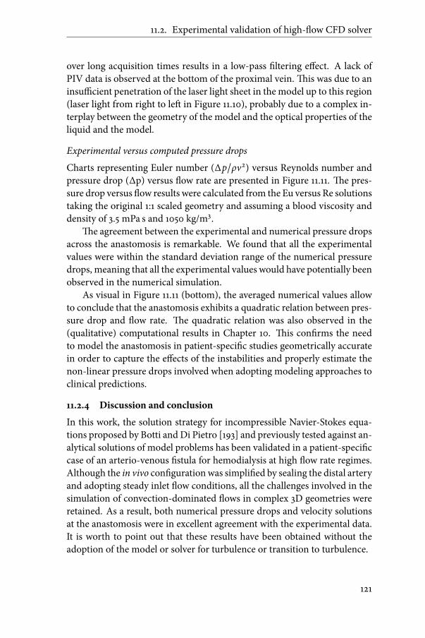
11.2. Experimental validation of high-�ow CFD solver
over long acquisition times results in a low-pass �ltering e�ect. A lack ofPIV data is observed at the bottom of the proximal vein.�is was due to aninsu�cient penetration of the laser light sheet in the model up to this region(laser light from right to le� in Figure 11.10), probably due to a complex in-terplay between the geometry of the model and the optical properties of theliquid and the model.
Experimental versus computed pressure dropsCharts representing Euler number (∆p/ρv2) versus Reynolds number andpressure drop (∆p) versus �ow rate are presented in Figure 11.11. �e pres-sure drop versus �ow results were calculated from the Eu versus Re solutionstaking the original 1:1 scaled geometry and assuming a blood viscosity anddensity of 3.5 mPa s and 1050 kg/m3.
�e agreement between the experimental and numerical pressure dropsacross the anastomosis is remarkable. We found that all the experimentalvalues were within the standard deviation range of the numerical pressuredrops, meaning that all the experimental values would have potentially beenobserved in the numerical simulation.As visual in Figure 11.11 (bottom), the averaged numerical values allow
to conclude that the anastomosis exhibits a quadratic relation between pres-sure drop and �ow rate. �e quadratic relation was also observed in the(qualitative) computational results in Chapter 10. �is con�rms the needto model the anastomosis in patient-speci�c studies geometrically accuratein order to capture the e�ects of the instabilities and properly estimate thenon-linear pressure drops involved when adopting modeling approaches toclinical predictions.
11.2.4 Discussion and conclusion
In this work, the solution strategy for incompressible Navier-Stokes equa-tions proposed by Botti and Di Pietro [193] and previously tested against an-alytical solutions of model problems has been validated in a patient-speci�ccase of an arterio-venous �stula for hemodialysis at high �ow rate regimes.Although the in vivo con�guration was simpli�ed by sealing the distal arteryand adopting steady inlet �ow conditions, all the challenges involved in thesimulation of convection-dominated �ows in complex 3D geometries wereretained. As a result, both numerical pressure drops and velocity solutionsat the anastomosis were in excellent agreement with the experimental data.It is worth to point out that these results have been obtained without theadoption of the model or solver for turbulence or transition to turbulence.
121

11. Experimental validation
Eu
Re
ExperimentalComputational∆
p (
mm
Hg
)
Q (ml/min)
ExperimentalComputational
Figure 11.11: Reynolds number versus Euler number (top) and equivalent bloodpressure drop versus �ow rate (bottom).
122

11.2. Experimental validation of high-�ow CFD solver
A�er successful validation of the proposed solution strategy for simu-lations in realistic geometries at high �ow regimes, the solver can now beemployed to reliably predict �ow patterns and pressure drops in patient-speci�c models of vascular access in patients on hemodialysis. More in gen-eral, the solver, here validated, may be useful for the numerical analysis ofother vascular beds that are characterized by high-�ow and blood veloci-ties associated with alteration of vascular geometry such as atheroscleroticplaques, bifurcations and branching as well.
123


Chapter
12Diagnostic tools
K. Van Canneyt, R.N. Planken, S. Eloot, P. Segers and P. Verdonck.Experimental study of a new method for early detection of vascular access
stenoses: Pulse pressure analysis at hemodialysis needle.Arti�cial organs. vol.34. 2010:113-117.
K. Van Canneyt1, A. Swillens1, L. Lovstakken, L. Antiga, P. Verdonck andP. Segers.
�e accuracy of ultrasound volume �ow measurements in the complex �owsetting of a forearm vascular access.
Revision submitted.
1Both authors equally contributed.
125

12. Diagnostic tools
12.1 Pulse pressure analysis for stenosis detection
12.1.1 Introduction
Complications of the vascular access (VA) for hemodialysis are amajor causeof morbidity and mortality in end-stage renal disease (ESRD) patients [19,199], with thrombosis due to �ow limiting stenosis being the main origin ofVA-failure [31, 200, 201]. �e Kidney Disease Outcomes Quality Initiative(K/DOQI) clinical practice guidelines de�ne a stenosis as relevant when itshows at least a 50%diameter reduction, accompanied by a hemodynamic orclinical abnormality [19, 199]. However, signi�cant �owdecline and increasein pressure drop appear only when the diameter is reduced to above 70%,and these criteria are therefore a late sign of stenosis development (Exam-ple in Figure 8.6 (p.61)).�e current vascular access surveillance techniques(�ow measurements and static-access pressure measurement) are thus un-able to detect relevant stenoses (<50% diameter reduction) in an early stage,and these methods cannot further reduce the incidence of vascular accessfailure due to thrombosis [120, 202–206].Up to date, monthly measurement of access �ow is considered the best
available surveillance tool for identi�cation of patients at risk of access throm-bosis [19, 199]. However, access �ow shows variation between and withinhemodialysis sessions [207]. Measurement of mean intra-access pressuresis more straightforward and can be performed using pressure transducerswithin the dialysis machine [202, 208]. Intra-access pressures re�ect ves-sel resistance and can be measured at the site of cannulation in the arterialand venous needle. However, current pressure measurements techniquesand protocols are tedious, time consuming, and not ‘user friendly’. Sta� fre-quently bypasses crucial steps (calibration, appropriate �ushing, etc.), lead-ing to poor quality data being collected and recorded [19, 199]. �erefore,monitoring techniques should be cheap, accurate, precise and easy to per-form.�e high thrombosis rates of arterio-venous �stulas and gra�s in par-ticular, require a sensitive and speci�c test that can unequivocally predictthe likelihood of thrombosis over a speci�c time. A combination of meanintra-access pressure and �ow measurements results in better prediction ofaccess thrombosis. However, the sensitivity of a combined surveillance pro-tocol for prediction of access thrombosis is only 73.3% and 68.8% in AVFand AVG, respectively [204].To overcome the inability to predict early stage stenoses (<50 diameter
reduction) and the low sensitivity of currently used tests, a non-invasive andinexpensive method based on the analysis of the pressure waveform pro�leand amplitude (PPA; pulse pressure analysis) is here extensively tested.�e
126

12.1. Pulse pressure analysis for stenosis detection
method was assessed using a dedicated in vitro model of a radio-cephalicarterio-venous �stula (AVF).
12.1.2 Material and Methods
�e vascular access model was integrated in a closed circuit (Figure 12.1). Ablood mimicking �uid is pumped from a reservoir into a windkessel by apulsatile pump (Harvard Apparatus, Bloodpump 4021, Model 55-3339, Hol-liston, USA).�is creates a system where the pump represents the le� ven-tricle and the windkessel the large central systemic arteries. From the wind-kessel, the �uid is distributed over themodel and over a draining tube with aresistance representing the blood �ow towards the body (except to the arm).A water-glycerin mixture at 25○C was used to mimic blood, with a kine-
matic viscosity of 3.2 10−6m2/s as measured with a capillary Ubbelohde vis-cometer (Schott, Germany) and a density of 1090 kg/m3. �is resulted in a�uid with a dynamic viscosity of 3.49mPa.s, corresponding to blood with ahematocrit of 42% [117].In the vascular access model, the artery was connected to the draining
vein (angle 60○). �e internal diameters of the artery and vein were 4mmand 7mm, respectively.�e arterial compliance was 8.2 10−7ml/Pa/cm [209,210], while the venous compliance was 46.0 10−7ml/Pa/cm (Unpublisheddata).�ese di�erent compliance values were achieved by constructing thedi�erent vessels with an appropriate number of silicon layers to obtain com-pliances in the physiological range.Tomimic the hemodialysis setting, two 15Gauge needles (BionicMediz-
intechnikGmbH, Frankfurt, Germany)were introduced.�e arterial needlewas inserted against the direction of �ow 5 cm downstream the anastomo-sis and the venous needle was inserted along the �ow and 5 cm more distal(Figure 12.1). Both needles were punctured and entered the siliconmodel for1 cm by an angle of approximately 30 degrees.�e introduced stenoses weremade of rigid tubes with a length of 1 cm. Stenosis of 25% and 50% diameterreduction were placed on three di�erent locations: (I) 10 cm proximal to theanastomosis (’proximal artery (PA) stenosis’); (II) in between the two nee-dles (’distal vein (DV) stenosis’); (III) 3 cm distal to the needles (’proximalvein (PV) stenosis’). So the DV-stenosis was located 3.5 cm downstream thearterial needle tipwhereas the PV-stenosis was located 9 cmdownstream theneedle tip. See also Figure 12.1, which indicates the position of the stenoses.For each case, the initial boundary conditions were set before introduc-
ing any stenosis in the following manner.�e �ow towards the vascular ac-cess model was established using both the adjustable resistance towards thearm and the rest of the body (Figure 12.1).�e �ow in the artery was divided
127

12. Diagnostic tools
Figure 12.1: Vascular access model integrated in mock loop (⋆ : stenosis locations)
into 90% towards the vein and 10% towards the distal artery, adjusting theoutlet resistance of the vascular access model.�e inlet pressure pro�le wasmeasured in the proximal part of the artery and the air level in the wind-kessel was regulated such as to establish a pro�le with a pulse pressure (PP;systolic minus diastolic pressure) of about 40mmHg.Starting from the reference situation described above (no stenoses, 90%
venous �ow and 10% distal artery �ow), the two di�erent stenoses were suc-cessively introduced at the three positions, and for each case arterial blood�ow (500-1300ml/min) and heart rate (60; 75 and 90 beats/min) were var-ied.
�e pulse pressure at the proximal part of the artery (PPPA) and at thearterial needle (PPAN ) was measured using �uid �lled pressure transducers(type DT-X PLUS, Becton Dickinson, New Jersey, USA).�e signal was ac-quired at a sampling rate of 200Hz and displayed on screen using dedicateddata acquisition hard- and so�ware (National Instruments, Austin, USA).�e values of PP used for analysis were the average of at least 6 cycles. A
128

12.1. Pulse pressure analysis for stenosis detection
dimensionless factor, ’%-Pulse Pressure’ (%PP), was de�ned as:
%PP = 100 ⋅ PPANPPPA
(12.1)
�e pulse pressure analysis, PPA, consists of a comparison of the %PP mea-sured in the di�erent cases.
Statistical analysisData are generally given as mean± standard deviation, with data averagedper case (a given stenosis percentage at one given location) over the mea-sured range of heart rate and blood �ow. Analysis of variance (ANOVA)was performed to obtain a statistical ground to evaluate the PPA-method ondetecting the presence of a stenosis, and discriminating between the loca-tions of the stenosis. Post-hoc (Bonferroni) tests were used to assess detailson which cases are di�erent from each other in terms of %PP. Linear regres-sion analysis was used to assess the relation between%PP and hemodynamicvariables.
12.1.3 Results
Arterial blood �ow rate versus %PP for the 50% stenosis is shown in Fig-ure 12.2a.�e %PP decreases with increasing blood �ow and increases withincreasing heart rate. In the control model (no stenosis), %PP was 20.26± 4.55. A stenosis in the proximal artery signi�cantly decreased %PP to 7.69± 2.08 (P < 0.0001), while presence of a stenosis in the venous part of themodel increased %PP, with values of 36.20 ± 2.12 for the DV-stenosis and32.38 ± 2.17 for the PV-stenosis (all P < 0.0001 compared to control). Whenapplying the analytical formulation of the regression curves for an arterialblood �owof 800ml/min (themean value of blood �ow in the experiments),the control case gives a %PP of 22.11. When we compare this to the PA-case,this value decreases to 6.80. For the stenoses distal to the needle, the%PP in-creases to 33.51 for the PV-stenosis and 36.92 for the DV-stenosis.�e post-hoc analysis shows that the %PP is signi�cantly di�erent for the 50% stenosisupstream versus downstream of the needle (P < 0.0001). It is even possibleto distinguish between the distal and the proximal vein stenosis (P < 0.0001).Figure 12.2b shows the results for the 25% stenosis case, where %PP de-
creases from 20.26 ± 4.55 (control) to 15.45 ± 2.13 (p = 0.0022) for the PA-stenosis, while it increases a�er introduction of the DV-stenosis to 26.71± 3.01 (p = 0.0003) and to 26.53 ± 2.67 for the PV-stenosis (p = 0.0004).�epost-hoc analysis shows that%PP for the 25% stenosis discriminates betweenthe upstream and downstream location (P < 0.0001), but it is not possible todistinguish the distal from the proximal vein 25% stenosis.
129

12. Diagnostic tools
Figure 12.2: %-PP for varying arterial blood �ow rates: (a) 50% stenosis cases fordi�erent heart rates versus the no-stenosis case; (b) 25% stenosis cases (-⋅- proximalartery, – proximal vein and ⋅ ⋅ ⋅ distal vein stenosis) with heart rate of 60 bpm versusthe no-stenosis case.
130

12.1. Pulse pressure analysis for stenosis detection
12.1.4 Discussion
�ere is an urgent need for a method that detects stenoses in early-stage inhemodialysis patients to prevent stenosis-related vascular access complica-tions. In this work, we have presented a method, based on analyzing thePP at the hemodialysis line, and tested the method in an experimental hy-draulic bench model setting. Hans-Dietrich Polaschegg stated in his patent[211, 212] that pulse pressure might be a method to detect stenosis, howeverno investigations or in-depth analysis on the method was performed. Al-though the basic principle of using pulse pressure is the same, the studiedmethod in this work is unique.Our experimental results for a 25% and 50% stenosis con�rm what has
earlier been described by Stergiopulos et al. using a computer model of thearterial tree to study the e�ect of arterial stenoses [209]. When the PP ismeasured proximal to the stenosis and compared with the PP in the casewithout stenosis, it increases, while the PP decreases when it is measureddistal from the stenosis.�is trend is con�rmed for all positions of the steno-sis.For the reference and 50% stenosis case, a clear e�ect of the heart rate
and the arterial blood �ow rate can be observed on the values of %PP (seeFigure 12.2, panels a and b). We have tested the method over an anticipatedrange of heart rates and blood �ow, and treated the measured data as inde-pendent samples, without accounting for the covariance e�ect of �ow andheart rate. As such, the statistical test we applied is more conservative thanan analysis of covariance, which would also account for the relationship be-tween%PP and heart rate and blood �ow. We feel that this approach is closerto the clinical reality, where at least the �ow level is not known either. De-spite this conservative approach, %PP was found to discriminate betweenthe three locations for the 50% stenosis, and between upstream and down-stream stenosis of the PA needle for the 25% stenosis. As such, we feel thatthe fact that heart rate and arterial blood �ow rate may vary in a clinical set-ting, this does not jeopardize the power of the PPA for detection of stenosesin the di�erent stenosis cases.In experimental modeling, it is necessary to establish a ‘reference’ situa-
tion and report ‘normalized’ results, with changes from this reference posi-tion. From a clinical point of view, the in vitro nature of the study is themainlimitation.�e value of the proposedmethod of PPAwill increase if it can beclinically proven that only the measurement of the PP at the needle (PPAN )makes the stenosis detection method accurate and sensitive. �e arterialpulse pressure could, for instance, be obtained from the brachial sphygmo-manometer cu� or using techniques of applanation tonometry. Anyhow, an
131

12. Diagnostic tools
inexpensive and ‘user friendly’ surveillance technique will only be obtainedif the PP at the needle can be calculated directly within the dialysis machine,as for intra-access static pressure measurements. Beside these remarks, an-other limitation of the experimental model is the fact that it is a simpli�-cation of the human vascular system. Human vessels react on blood �owand pressure changes by vasodilation or vasoconstriction in an acute settingand structural remodeling in the longer term. When the method is used indaily clinical practice, these changes in the cardio-vascular system may in-terfere with the pressure pro�le analysis.�erefore a clinical trial should beperformed to validate this detection method.
12.1.5 Conclusion
We have extensively in vitro tested a method, based on analysis of the pulsepressure, enabling detection of the presence and location of a 50% stenosisindependent of heart rate and arterial blood �ow rate. Nevertheless, a clin-ical study will have to con�rm these experimental results and the potentialof this low-cost method.
132

12.2. �e accuracy of ultrasound volume �ow measurements
12.2 The accuracy of ultrasound volume flow measurements
12.2.1 Introduction
In Europe, more than half-a-million patients with end-stage renal disease(ESRD) are treated with hemodialysis and this population still increases an-nually by approximately 5-8% [9–12]. Tomake hemodialysis possible, a well-functioning vascular access is needed to facilitate high blood �ow and to al-low repeated cannulation over time [21, 25].�e preferred vascular access iscreated by surgically connecting an artery and a vein in the arm (an arterio-venous �stula; AVF). Ideally, the AVFmatures, resulting in the required �owincrease and vascular remodeling to allow for dialysis [21, 25, 26]. Despite theextensive preoperative examinations, non-maturation occurs in 23 to 46% ofthe cases [36, 37].Direct postoperative �owmeasurements can be linked, in an early-stage,
with the non-maturation in case of a too low �stula �ow and with distal is-chemia and cardiac failure in case of a too high �stula �ow [26, 32, 44, 164,167]. �e ideal method to measure the �ow rates should be non-invasive,workable in daily clinical practice and reproducible. Nowadays, one of themost widely available methods is based on pulsed wave Doppler (PWD) ul-trasound (US), where PWD provides velocity information that is multipliedwith an estimate of the cross-sectional area of the vessel to obtain volumetric�ow.Although PWD is a well-established method to measure �ow velocities,
it has some intrinsic limitations.�emost important one is the 1D-nature ofthe measurement, since PWD only captures the velocity component in thedirection of the US-beam.�e translation of this 1D velocity measurementto the full cross-sectional velocity pro�le, in order to estimate the �ow rate,requires a great number of assumptions.�ese uncertainties involved in the�ow rate calculation are expected to increase signi�cantly when a disturbedand complex �ow �eld is introduced, as one may expect post AVF-creation.So, despite the fact that the PWD �ow estimation is non-invasive and usedon large scale in daily routine, the reproducibility, intra- and inter-observervariability, and the accuracy remain unclear [213–217].In this study, we want to assess the accuracy of the �ow rate as mea-
sured by US compared to the actual �ow rate present in the setting of AVF.To ensure that we have gold standard information on the true velocity �eldmeasured by pulsedwaveDoppler, wewill follow an approach based onmul-tiphysics simulations, integrating computational �uid dynamics with an ul-trasound simulator. Aswe demonstrated before, thismodeling technique al-lows to simulate synthetic but realistic ultrasound images, based on a known
133

12. Diagnostic tools
but complex 3D-�ow situation [218, 219]. As such, we will produce syntheticPWDspectra to derive �ow rates, which can then be compared to the groundtruth values known fromCFD. For this analysis, two patient-speci�c geome-tries of one AVF patient, based on pre- and postoperative MR-images of thearm vasculature, will be used.
12.2.2 Material and methods
Multiphysics simulations to generate synthetic pulsed wave Doppler data
(a) Flow simulations in a patient-specific model of AVF usingcomputational fluid dynamics (CFD)Two sets of high-resolutionMR angiography images were acquired from thesame patient (51 year old, male, BMI 20.5), one set preoperatively and one15 weeks a�er AVF creation. From these MR data sets, both a preoperativeand a postoperative 3D-model were reconstructed.�e preoperative modelconsists of the brachial artery, which bifurcates into the ulnar and the radialartery (Figure 12.3, top).�e postoperative model additionally includes thearterio-venous anastomosis and the distal cephalic vein (Figure 12.3, bot-tom).�e in�ow segment was arti�cially prolonged for both pre- and post-operative models to ensure fully developed �ow conditions (independent ofthe boundary conditions) at sites of �ow investigation. To avoid disturbanceof the distal high �ow vortices in the postoperative model, straight out�owsegments were added as well.
�e two geometries were segmented from the MR images, using theopen-source so�ware vmtk2.�e model was meshed using pyFormex3, ac-cording to themethods described by De Santis et al. [220, 221]. A conformaland structured hexahedral mesh was applied on the models, resulting in 1.4million cells for the preoperative case and 2.2 million cells for the postoper-ative case. Amesh-sensitivity analysis was performed to ensure that velocity�elds were obtained independent of the mesh density.A parabolic velocity pro�le was implemented as inlet boundary condi-
tion at the proximal brachial artery. �e pro�le was determined based onthe pre- and postoperative MRI Q-�ow acquisition from the selected pa-tient, but was rescaled such that a mean �ow rate of 100ml/min preoper-ative and 1000ml/min postoperative were obtained. �e ulnar artery re-ceived 40ml/min in both the pre- and postoperative case, and the distal ra-dial artery 60ml/min. For the postoperative case, this results in a �ow of
2http://www.vmtk.org3http://pyformex.org
134

12.2. �e accuracy of ultrasound volume �ow measurements
Figure 12.3: Pre- and postoperativemodel with indication of the assessed locations,boundary conditions and �uid properties.
900ml/min going through the vascular access, which is in range with clin-ical practice and the European and American guidelines for vascular access[19, 22].Blood was modelled as an incompressible Newtonian �uid with a den-
sity of 1050 kg/m3 and a viscosity of 3.5mPa.s. Rigid walls and no-slip con-ditions were set. Womersley numbers, α, de�ned as:
α = R√2π f ρ/µ (12.2)
(with R the radius of the vessel, ρ the density of blood, µ the viscosity ofblood and f the cardiac frequency), ranged from 1.8 to 3.3. For both geome-tries, two cardiac cycles were calculated to avoid transient e�ects, with a 5mstime step. Ansys Fluent 12 (ANSYS inc., Canonsburg, PA, USA) was usedto solve the Navier-Stokes equations with a �nite volume method. Standardpressure discretization and second-order upwindmomentum discretizationschemes were applied.
135

12. Diagnostic tools
(b) Ultrasound simulationsWe used the Field II so�ware [222, 223] to simulate the radiofrequent (RF)signals originating from the AVF blood �ow �elds. �is simulator is basedon the spatial impulse response estimation approach as proposed by Tupho-lme [224] and Stepanishen [225], and allows to model arbitrary transducersand scanning sequences with great �exibility. Field II represents blood as anensemble of random point scatterers on which the ultrasound waves re�ect.As such, realistic Doppler spectra were obtained by moving the point scat-terers during the simulated scanning procedure according to the AVF �ow�elds obtained from CFD. We implemented a realistic linear array trans-ducer for peripheral vascular applications, and RF-signals were obtainedby �ring 8000 and 22000 sinusoidal pressure pulses during the cardiac cy-cle, for the preoperative and postoperative case, respectively (pulse repeti-tion frequency (PRF) = 8/22 kHz, f0 = 5MHz, pulse length = 2.5 pulse peri-ods). �is higher pulse repetition frequency postoperatively was necessaryto avoid aliasing for the higher �ow velocities present in this setup. RF-datawere simulated at 2 locations (cfr. o in Figure 12.3): (i) the brachial artery,5 cm proximal to the radial-ulnar bifurcation (proximal location), and (ii)the radial artery, 5 cm proximal to the (location of the) anastomosis (dis-tal location). Finally, the Doppler sonograms were produced by choosingan appropriate depth and size of the sample volume, and applying Fourier-analysis to the simulated RF-signals. For more background on the ultra-sound simulator and the appliedmultiphysics simulation approach, we referto Swillens et al. [218, 219].
Volume �ow calculation based on pulsed wave Doppler spectra�e instantaneous volume �ow, Q(t), through a well-de�ned cross-section,A, can be calculated as the integration of the spatial velocity pro�le over thearea:
Q(t) =∬ (v(t) ⋅ n)dA =∬ vn(t)dA (12.3)
with v(t), the 3D-velocity vector in a certain point of the cross-section andn the direction of the normal of the cross-section A.�e projection of thevelocity vector v(t) on the normal n is denoted as vn(t). However, evalua-tion of this surface integral is highly cumbersome using conventional PWD,since it typically entails a range of assumptions, which are potentially erro-neous for complex �ow conditions.�e di�erent steps and according chal-lenges in correctly assessing Equation 12.3 are described below.
(a) Integrating over the cross-sectional area AEquation 12.3 shows that a correct measurement of the �ow, Q, requires
136

12.2. �e accuracy of ultrasound volume �ow measurements
knowledge of the spatial velocity distribution in the considered cross-section.As such, the most straightforward �ow assessment requires a direct mea-surement of this spatial velocity pro�le. However, conventional PWD sys-tems do not allow to simultaneously scan and process di�erent samplinglocations. Hence, directly assessing the spatial velocity pro�le is typicallycircumvented, and we investigated two commonly applied strategies in thismatter:(i) Equation 1 is simpli�ed to:
Q(t) = vn,mean(t) ⋅ A (12.4)
with vn,mean(t) the mean velocity in the considered cross-section, obtainedby stretching the Doppler sample volume (SV) over the complete cross-section [226]. �is method is further denoted as the large sample volumeacquisition.(ii)�e velocity is measured at a speci�c location of the cross-section
(typically the center point), and is further used to derive the spatial velocitypro�le by assuming the actual �ow conditions.�e �ow Q is then obtainedas:
Q(t) = β ⋅ vn,max(t) ⋅ A (12.5)with β a correction factor that accounts for the shape of the velocity pro�le;vn,max(t) the velocity in the center of the vessel cross-section and assumedto be the maximal velocity (as is the case for fully symmetrical �ow). A �at(β=1) or parabolic (β=0.5) pro�le are o�en assumed, but more complex �owpro�les can be derived using Womersley theory. �e β-factor for Womer-sley theory will be further indicated as βα . �is method was simulated bypositioning a small sample volume (SV= 0.39mm) in the center of the cross-sectional area.�is approach is further denoted as the small sample volumeacquisition.Another potential errorwhen estimatingQ is the assessment of the cross-
sectional area A, which is typically obtained from a simple measurement ofthe diastolic diameter (πD2/4), hence assuming a circular shape of the cross-section. As such, we also assessed the diameter at the assessed locations, butdirectly from the 3D reconstructed vascular geometry, since rigid walls wereassumed in the CFD-simulations.
(b) Assessment of vn(t): angle correctionUsing a mean frequency estimator, the velocity in the US-beam direction,vPWD, was derived from the Doppler spectra [226]. To reduce the varianceof the spectrum estimates, the �nal velocity curve was obtained by averag-ing power spectra from several individual range samples within the samplevolume.
137

12. Diagnostic tools
Although this mean frequency estimator theoretically results in unbi-ased velocity estimates vPWD [226], we also derived vPWD by tracking theouter contour (envelope) of the spectrum based on image intensity (cfr. Fig-ure 12.4). �is is a common approach in clinical practice because it is lesssensitive to shi�s inmeasurement location compared to themean frequencyestimation [168, 227]. In the remainder of this paper, wewill refer to vPWD(t)as obtained from respectivelymean-tracking ormax-tracking to indicate thedi�erence.Finally, the Doppler velocity vPWD was converted to the angle-corrected
velocity vn(t) as:
vn(t) =vPWD(t)cos(θ) (12.6)
With θ the angle between the ultrasound beam and the assumed �ow direc-tion. In this study, θ was set to 70○.
12.2.3 Results
Simulated Doppler spectraFigure 12.4 shows the PWD-spectra when the small sample volume is po-sitioned in the center of the cross-section (top-middle) and when a largesample volume covering the full cross-section was chosen, with both mean-tracking (solid white line) and max-tracking (dashed white line) visualized.For the postoperative case, the complex �ow conditions with high velocitymagnitudes result in increased spectral broadening and less smooth veloc-ity curves, with a larger di�erence between mean- and max-tracking curvesthan for the preoperative case. For the large sample volume, the lower ve-locities near the vessel wall are also picked up, as can be observed for thespectra in the lower panels of Figure 12.4.
Velocity from PWD versus CFDWe focus on two cases when comparing the results from the synthetic PWDspectra to the true �ow velocities (CFD):1. preoperative proximal (brachial artery in preoperative conditions), be-cause the �ow�eld in this region seems the least disturbed as it is closeto the straight in�ow section and demonstrates low �ow.
2. postoperative distal (radial artery in postoperative conditions) sincethe most complex �ow �eld was expected for this case
Figure 12.5 (top) compares the velocity as picked up by pulsed waveDoppler,vPWD, (in the direction of the ultrasonic beam), with the projection of theCFD velocity vector on this beam, vn. Results are demonstrated for a small
138

12.2. �e accuracy of ultrasound volume �ow measurements
Figure 12.4: PWD-spectra as obtained from the small sample volume acquisition(top-middle) for all four case and PWD-spectra obtained for large sample volumeacquisition (bottom) for the two preoperative cases. Mean-tracking (solid whiteline) and max-tracking (dashed white line) are indicated.
sample volume in the center of the cross-section. Comparison with theground truth shows that max-tracking of the Doppler spectrum results inan overestimation of the velocity (mean bias of +65.5% for the preoperativeand +46.4% for the postoperative case). �e mean-tracking, on the otherhand, shows a good agreement with the reference value obtained fromCFD,with a slight underestimation of PWD (mean bias of -3.3% preoperative and-8.1% postoperative).
139

12. Diagnostic tools
Preopera�ve
Proximal
Postopera�ve
Distal
Time [s]
Ve
loci
ty [
m/s
]
0 0.2 0.4 0.6 0.8 1
Time [s]
Ve
loci
ty [
m/s
]
1.1
0 0.2 0.4 0.6 0.8 10
0.1
0.2
0.3
0.4
0.5
0.6
0.7
0.8
0.9
1
0
0.5
1
1.5
2
2.5
3
3.5
4
4.5
5
5.5
6
6.5
1.1
0 0.2 0.4 0.6 0.8 10
0.1
0.2
0.3
0.4
0.5
0.6
0.7
0.8
0.9
1
Time [s]
Ve
loci
ty [
m/s
]
0 0.2 0.4 0.6 0.8 1
Time [s]
Ve
loci
ty [
m/s
]
0
0.5
1
1.5
2
2.5
3
3.5
4
4.5
5
5.5
6
6.5
CFD US mean-tracking US max-tracking
Velocity in beam direc�on: vPWD
(t)
Angle-corrected velocity: vn(t)
Figure 12.5: �e upper panels show the velocity as picked up by PWD (in theUS beam direction), with the mean-tracking in solid gray and the max-trackingin dashed gray.�e CFD ground truth is displayed in solid black.�e lower panelsshow the velocity a�er angle correction, with the same color coding as the upperpanels.�is comparison is illustrated for a small sample volume acquisition, in thepreoperative proximal (le�) and the postoperative distal region (right).
Figure 12.5 (bottom) compares the corresponding angle-corrected ve-locity vn, with the projection of the CFD velocity vector on the normal ofthe cross-section. �e angle correction further enforces the overestima-tion by the max-tracking (mean bias of +65.6% for vPWD and +99.1% forvn in the preoperative case). Angle correcting the mean tracking resultsin an overestimation preoperatively (bias=+16.3%) and an underestimation(bias=-14.2%) postoperatively.
Flow from PWD versus CFDFigure 12.6 shows the volume �ows obtained from the PWD spectra, for asmall sample volume acquisition (solid gray for mean-tracking, dotted gray140

12.2. �e accuracy of ultrasound volume �ow measurements
for max-tracking), assuming a Womersley �ow pro�le.�e applied correc-tion factors βα , according to Equation 12.5, where 0.658, 0.626, 0.658 and0.627 for preoperative proximal, preoperative distal, postoperative proximaland postoperative distal, respectively. While the proximalmeasurements (inthe brachial artery) show a clear overestimation by ultrasound, both for themean- and max-tracking, results are less univocal for the distal site (radialartery).
�e deviation between the simulated volume �ow measurements andthe ground truth is further quanti�ed in Table 12.1, providing an overviewof the bias on the ultrasound data for the small sample volume acquisition.Both mean- and max-tracking of the Doppler spectra are reported, as wellas di�erent assumptions on the velocity pro�le (parabolic �ow, Womersley
Flo
w r
ate
[m
l/m
in]
Po
sto
pe
ra!
veP
reo
pe
ra!
ve
Distal
Time [s] Time [s]
Proximal
Flo
w r
ate
[m
l/m
in]
0 0.2 0.4 0.6 0.8 10
100
200
300
400
500
600
700
800
0 0.2 0.4 0.6 0.8 1
0
50
100
150
200
250
300
350
400
450
0 0.2 0.4 0.6 0.8 1400
600
800
1000
1200
1400
1600
1800
0 0.2 0.4 0.6 0.8 1
500
1000
1500
2000
2500
3000
3500
CFDUS small SV
mean-tracking
US small SV
max-tracking
US large SV
mean-tracking
Figure 12.6: Volume �ows (solid gray = mean-tracking, dotted gray = max-tracking), for a small sample volume (SV) acquisition, calculated with the β-valuefromWomersley theory (Equation 12.5) are shown together with the volume �ows(dashed gray) for large sample volume (SV) acquisition (Equation 12.4), usingmean-tracking, are compared to the CFD �ow rate (solid black). Top: Preopera-tive cases; Bottom: Postoperative cases; Le�: Proximal cases; Right: Distal cases.
141

12. Diagnostic tools
�ow, plug �ow). Tracking the outer contour of the spectrum dramaticallyoverestimates volume �ow, except for the postoperative distal case (radialartery), where assuming a parabolic pro�le leads to an underestimation of-14.8%. Volume �ow obtained from mean tracking is also systematicallyoverestimated when assuming a plug �ow pro�le or a Womersley pro�le(except the postoperative distal case), but is underestimated when assum-ing parabolic �ow.
Small sample volume Mean PWD-tracking Max PWD-tracking% bias Parabolic Womersley Plug Parabolic Womersley Plug
preoperative Proximal -1.2 +30.1 +97.7 +69.2 +122.7 +238.4Distal -10.8 +11.7 +78.5 +40.8 +76.3 +181.6
postoperative Proximal -1.4 +29.8 +97.3 +59.2 +109.5 +218.3Distal -46.5 -33.0 +6.9 -14.8 +6.8 +70.4
Table 12.1: �e bias for the time-averaged �ow rate, in case of the small samplevolume acquisition. Flows were calculated based onmean- andmax-tracking of theDoppler spectrum, and di�erent assumptions on the spatial velocity pro�le wereinvestigated. β-values for a fully parabolic (β = 0.5), Womersley and plug (β = 1)�ow were applied.
Large sample volumeTo complete the analysis, the volume�ows for a large sample volume (dashedgray) with mean-tracking, calculated according to Equation 12.4 are shownin Figure 12.6.�esewere based onPWD-spectra as shown in the lower pan-els of Figure 12.4.�e bias of the simulated ultrasound data compared to theCFD values (comparing time-averaged �ows), is listed in Table 12.2. FromFigure 12.6 and Table 12.2, it is clear that the �ow rates are overestimated bythe US-algorithms, again, except for the postoperative distal case.
Large sample volume % bias
preoperative Proximal +67.6Distal +46.6
postoperative Proximal +14.2Distal -6.3
Table 12.2: �e bias for time-average �ow rate, in case of large sample volume ac-quisition.
142

12.2. �e accuracy of ultrasound volume �ow measurements
12.2.4 Discussion
In this paper, we studied PWD-based �owmeasurements in the brachial andradial artery in patients with an arterio-venous �stula, both in the pre- andpostoperative case. We demonstrated that these PWD-based �ow estimatesare subject to a high degree of inaccuracy. �is inaccuracy is not directlyrelated to the inability of PWD to accurately capture the velocity componentin the direction of the ultrasound beam, but is induced via two factors:1. the angle-correction, which does not correctly estimate the velocitycomponent along the assumed �ow direction
2. the lack of knowledge on the �ow pro�le�e inaccuracy induced by angle correction in volume �ow estimation isdemonstrated in Figure 12.7. It illustrates the process of angle-correctingthe PWD velocity, both for the case of uni-directional laminar �ow (= ve-locity vectors aligned with the axis of the vessel) and complex �ow (= ve-locity vectors no longer aligned with the axis of the vessel). In both cases,the velocity measured by PWD, vPWD (green), is the projection of the true3D-velocity vector v (black), on the direction of the ultrasound beam (eus).For uni-directional �ow (Figure 12.7, top), vPWD is the projection of the lon-gitudinal velocity, vx (blue), which in this case equals the velocity vector v.However, when a complex �ow �eld is present, vPWD not only consists ofa contribution from the longitudinal component vx (blue), but also fromthe radial vy component (red). As such, the angle-corrected Doppler ve-locity vn does not only re�ect the longitudinal velocity component vx butalso the radial velocity component vy. �erefore, depending on the �ow�eld and the orientation of the velocity vectors, angle-correction of vPWDcan either over- (Figure 12.5 (le�), preoperative, proximal) or underestimate(Figure 12.5 (right), postoperative, distal) the velocity in the assumed �owdirection (vn(t)).To illustrate that the orientation of the �ow vectors indeed plays a role
in the cases considered here, we display the �ow �elds and the in-plane ve-locity vectors for the four studied cases in detail in Figure 12.8. It is clearthat in all cases the in-plane velocity vectors have a non-zero component inthe radial y-direction, which is also picked up by the Doppler measurementas shown in Figure 12.7. For the preoperative proximal case, the velocityvectors point upwards, resulting in a positive velocity vy, while for the post-operative distal case, the velocity vectors in the sample volume (indicated inwhite) point downwards, resulting in a negative velocity vy. Note also thehighly asymmetric, skewed nature of the �ow pro�les in the postoperativecase.
143

12. Diagnostic tools
1. Projec�on of velocity on US-beam
2. Angle correc�on (θ)
vPWD = v’x
vn = vPWD / cos (θ)
= (v’x ) / cos (θ)
= vx !
vPWD
US-beam direc�on=
1. Unidirec�onal flow
US-probe
v = vx= vn
vPWD = v'x
yxUS eθsineθcoserrr)()( +=
1. Projec�on of velocity on US-beam
2. Angle correc�on (θ)
)(θsinvy ⋅+
v’x + v’y
US-beam direc�on=
2. Complex flow
US-probe
v
vx
vy
v'xv'y
vPWD
vn
yxUS eθsineθcoserrr)()( +=
vPWD =
vPWD
)θcosvv x (⋅eUS⋅rr
= =
)θcosvv x (⋅eUS⋅rr
= =
vn = vPWD / cos (θ)
= (v’x ) / cos (θ)
vx !
+ v’y
yer
xer
zer
θ
θ
yer
xer
zer
θ
=
Figure 12.7: Illustration on why angle correction of the Doppler velocity works forunidirectional �ow (upper case 1) but fails for complex �ow (lower case 2).
Beside the angle-correction itself, the method applied to derive the ve-locity curve from the Doppler spectrum can introduce considerable errorsin the �ow estimation.�emaximum frequency detector is seriously biased,as noticeable in Figure 12.4, since the maximum frequency cannot be uni-vocally determined because of intrinsic spectral broadening processes [226].�erefore, although it is a common approach in clinical practice [168, 227],due to the lower sensitivity to shi�s in measurement location, the max-tracking leads to signi�cant overestimation of the actual �ow velocities and�ows. Further, it should be noted that while max-tracking is usually per-formed by analyzing pixel intensity, mean-tracking requires direct access tothe spectral estimates and thus registration of the RF-data during the mea-surement.Further, the lack of knowledge on the spatial velocity pro�le contributes
to the inaccuracy of the �ow estimation. When assessing the velocity in asample volumepositioned in the center of the cross-section, a correction fac-tor β needs to be assumed, which relates to the shape of the velocity pro�le.Our data seem to indicate that, for the investigated cases, there is no single
144

12.2. �e accuracy of ultrasound volume �ow measurements
Postopera�ve
Preopera�ve
DistalProximalyer
zer
Figure 12.8: Velocity magnitude [m/s] in the four selected region of interest withthe in-plane velocity vectors at the time point of peak velocity. �e small samplevolume (0.39mm) is shown in white.
optimal choice for β.�e β-values that one should use to match the PWD-derived velocity data, analyzed by mean-tracking, to the true mean velocityknown from CFD are 0.506, 0.560, 0.507 and 0.935 for preoperative prox-imal, preoperative distal, postoperative proximal and postoperative distal,respectively. In the proximal locations, the assumption of a parabolic �owpro�le for a small centered sample volume (β = 0.5) seems reasonable. Forthe distal location in the small sample volume acquisition, the theoreticalvalue ranges from0.560 to 0.935 when changing from the pre- to the postop-erative model. It is clear that the increase in overall �ow rate induces a morecomplex �ow pattern, see Figure 12.8, with a β value closer to the solutionfor plug �ow. As stated before, the max-tracking signi�cantly overestimatesthe �ows. �is results in ideal β-values of about 0.6 for the postoperativedistal case and about 0.33 (1/3th) for the other three cases.
145

12. Diagnostic tools
In the assumption of fully symmetrical �ow pro�les, one expects thatthe use of the larger sample volume, using mean-tracking (Equation 12.4),should provide the most accurate estimate of the volume �ow. Interestingly,our data indicate that this was not systematically the case. First of all, thismethod is challenged since the velocities in the vessel wall region are di�cultto measure, even in straight vessel segments [228–232]. Furthermore, thismethod only assesses the mean velocity of the 1D velocity pro�le, instead ofassessing the mean velocity for the complete 2D cross-section.
�e cross-sectional area used for the PWD �ow estimate was calculatedbased on the diameter measured perpendicular to the vessel assuming a cir-cular cross-section.�ese estimated areas only di�ered 2.2%, 2.0%, 6.0% and2.4%, for preoperative proximal, preoperative distal, postoperative proximaland postoperative distal respectively, with the 2D-cross-sectional areas cal-culated from the CFD solution.�erefore, the cross-sectional area calcula-tion is, when comparing to the overall �ow estimation bias in Table 12.1-12.2,no major source of error in our evaluation.As described by Swillens et al., the use of multiphysics ultrasound sim-
ulations bears some inherent limitations, the most important being the as-sumption of linear ultrasound wave propagation, the use of rigid walls andthe absence of surrounding tissue, the latter typically a�ecting the accuracyof blood velocity estimation [219].�e result of a velocitymeasurement withultrasound is also dependent on the probe settings. �e simulations wereperformed for a typical linear array probe used for vascular examinations,with PRF-settings that were tuned to allow capturing the maximum veloci-ties as one would do in clinical practice. We believe that our speci�c choicehas only a minor in�uence on the overall message and conclusion of thisstudy. However, an in-depth analysis of probe settings and imaging param-eters, coupled with di�erent �ow regimes, could provide more inside in thecomplex nature of PWD acquisitions. �is could be included in a futurelarge parameter study.It is clear that, based on our study, it is di�cult to provide strict guide-
lines to estimate blood �ow rate by PWD-acquisition. Overall, for the inves-tigated cases, measurements based on the small sample volume positionedin the center of the vessel, analysis based on mean-tracking and with the as-sumption of a parabolic �ow pro�le showed greatest accuracy, except for thedistal measurement in the postoperative case where the method underesti-mates �ow by about 50%.From a clinical perspective, it might be safer to apply a method which
leads tomore conservative (underestimated) values of �ow rather thanmeth-ods leading to overestimation, although the better method performs well
146

12.2. �e accuracy of ultrasound volume �ow measurements
under all circumstances. More robust techniques are available when record-ing �owduring hemodialysis therapy, based on connecting the patient to theextra-corporal circuit (e.g. ultrasound �ow dilution (Transonic)). When as-sessing preoperative or direct postoperative �ow, replacing PWD derived�ow measurements can be more cumbersome. However, it should be notedthat more advanced ultrasonic �ow estimators are being developed, but arestill in a preclinical phase. A potential solution for the demonstrated lim-itations regarding PWD volume �ow measurements, is the use of 2D �owestimators (e.g. speckle tracking, vector Doppler) [233–243], avoiding theneed to angle correct a 1D velocity, but their clinical applicability is to bedemonstrated. In parallel, researchers have focused on the development ofmulti-gate Doppler acquisitions, allowing to directly assess the velocity pro-�le, through simultaneous processing of several sample volumes along theUS beam [244].
12.2.5 Conclusion
We conclude that, in the setting of a forearm vascular access, �ow estimatesbased on pulsed wave Doppler are hampered by the complex �ow patterns,especially in the postoperative setting. Flow estimation based on centerlinemeasurement, analysed by mean-tracking of the spectral estimates and un-der the assumption of a parabolic �ow pro�le seem to provide reasonablevalues for most cases.
147


Four
Study on AVGs
149


Chapter
13Computational study of flow in
helical AVGs
K. Van Canneyt, U. Morbiducci, S. Eloot, G. De Santis, P. Segers andP. Verdonck.
A Computational Exploration of Helical Arterio-Venous Gra� Designs.Revision submitted.
151

13. Computational study of flow in helical AVGs
13.1 Introduction
Nowadays, over 20 million patients worldwide are in need of renal replace-ment therapy [10, 11]. In western countries, over 90% of the patients waitingfor a kidney transplant depend on hemodialysis [12, 17], and need a long-term vascular access. Although an arterio-venous �stula (AVF) is the �rstchoice in most patients, in speci�c cases (e.g. low quality vessels in elderlyor diabetics) an arterio-venous gra� (AVG) is the second best option [245].Hereby an artery and a vein, mostly in the (lower) arm are connected by asynthetic gra�.AVGs, however, deal with complications such as thrombosis and steno-
sis formation. As clinically observed, the stenosis formation with AVGs ismainly located at the venous anastomosis or in the draining vein [30, 75,246]. �ese adverse events, due to maladapted intimal hyperplasia (IH)[30, 36], are driven by abnormal hemodynamics. It is known from literaturethat, a�er vascular access creation, the �ow �eldmay play amodulating role,with IH mainly located in regions of low wall shear stress, high oscillatoryshear stress and high residence time [75, 124, 125, 246–250]. Furthermore,certain �ow patterns in the bulk, induced by out-of-plane geometries, canbe linked to disturbed shear distributions at the luminal surface [71–73, 251].More speci�cally, helical �ow tends to reduce these unfavorable hemody-namic conditions [128, 252–255].With this in mind, a helical shape was introduced in AVG designs by
Caro et al. [70, 74]. Up to now, the research on helical AVGs as vascularaccess consists of an animal model study [74], a preliminary clinical studyon 20 patients [76], and a clinical trial on 180 patients, as suggested in thework by Glickman et al. [77]. In other studies, computational �uid dynam-ics (CFD) was applied to analyze the hemodynamic performances of helicalgra�s in a stand-alone [256, 257] and in a bypass con�guration [258], notonly to minimize disturbed shear but also to improve near wall and cen-tral �ow mixing. Sun et al. compared the helical gra� design from Caro etal. [74] with a new helical design, using steady-state �ow conditions [256].Cookson et al. investigated the in-plane �ow structures and central �owmixing in helical conduits in steady-state �ow conditions [259]. Coppolaand Caro investigated the impact of arterial three-dimensionality on bothwall shear stress and oxygen transport/transfer [73]. Zheng et al. simulatedsteady �ows in helical gra�s and carried out a parametric analysis with re-spect to the Dean Number and helical pipe geometric features, i.e., helicalpitch and amplitude [257]. Recently, Zheng et al. simulated the physiologicalpulsatile �ow in helical gra�s and observed that helical geometry creates am-pli�ed WSS magnitudes near the wall, that oscillatory shear never exceeds
152

13.2. Material and methods
non-physiologically signi�cant values, and that the strong secondary �owsimprove �ow mixing between low-momentum �uid near the surface andhigh-momentum �uid near the central �ow [260]. Only Wen et al. studiedthe gra� in a coronary bypass setup (low �ow, small diameter, no loop) andone helical design was compared to the straight conventional design [258].So, while di�erent computational studies have been performed in low �ow(coronary) bypass con�gurations or in stand-alone con�gurations without(arterial or venous) anastomosis, up till now, the clinically relevant, high�ow, helically-designed loop AVG con�guration has not been studied in de-tail [75].
�erefore, the aimof this studywas to investigate, usingCFD, the impactof the introduction of helical design in an AVG loop as a vascular access forhemodialysis on the occurrence of (un)favorable hemodynamic conditionsat the venous anastomosis [30, 75, 246].
13.2 Material and methods
Six di�erent parametric models of a gra� connecting an artery and a veinwere created in pyFormex1. All models consist of a 4mm (diameter) artery,a 6mm gra� section and a 6mm vein, as shown in Figure 13.1. �e gra�section has a length of 300mm in a loop con�guration with both anasto-mosis angles set at 45 degrees. As a reference model, a straight conventionalgra� (SCG) was constructed. As shown in Figure 13.2, �ve helical designgra�s (HDG-1 to HDG-5) were created to analyze the in�uence of a helicaldesign on hemodynamics.�e amplitude of the helix of the gra� was 3mm(half the gra�’s diameter) and one helix turn (pitch) was 105mm; 87.5mm;70mm; 52.5mm or 35mm long, respectively. HDG-3 is based on the designof the SwirlGra� (Veryan Medical Limited, UK).
�emodels were discretisedwith a fully conformal and structured hexa-hedral mesh [220, 221, 261]. Because of the high �ow rates and the expectedtransitional �ow patterns [262], an extensive mesh density and time stepanalysis was performed. 200Hz sampling and consecutive mesh re�nementup to 4.3million cells (4.5million nodes) resulted in WSS values at the ve-nous anastomosis regionwithin 2% of the results obtainedwith a 6.4millioncell model. With the used hexahedral meshed meshes, about 140 hours, on24 nodes of an in-house cluster, were required to calculate two consecutivecardiac cycles, for one model.
1http://pyformex.org
153

13. Computational study of flow in helical AVGs
0 0.2 0.4 0.6 0.8 10
500
1000
1500
Time [s]
Infl
ow
ra
te [
ml/
min
]
Conformal and structured
hexahedral mesh
Quemada viscosity model
(shear thinning)
Density: 1050 kg/m³
Velocity inlet
5%
5%
90%
4mm artery6mm vein
6mm gra"
300mm gra" length
45° angle
Mean inflow rate
600 ml/min
(200Hz sampling)
Parametric model:
up to 4.3 million cells
(4.5 million nodes)
ROI-1
ROI-2
Figure 13.1: Summary of model, mesh, material properties and boundary condi-tions (example of HDG-3). Region of interest at venous anastomosis site (ROI-1)and region of interest in gra� section (ROI-2) are highlighted.
�e �nite volume method was applied to solve the laminar governingequations of the �uidmotion, by use of the general purpose CFD codeAnsysFluent 12 (ANSYS inc., Canonsburg, PA, USA).A post-operative �ow waveform from a vascular access patient was ac-
quired by use of magnetic resonance imaging as described by Huberts et al.[168]. A patient-speci�c �ow waveform was set, in terms of parabolic veloc-ity pro�le, as inlet boundary condition at the proximal artery (Figure 13.1).�e pro�le was scaled to achieve a time-averaged �ow rate of 600ml/min,which is in line with the European and American guidelines on vascular ac-cess [19, 22].�e in�owwas redistributed such that 95% was sent to the gra�(with a further downstream division of 90% of to the proximal vein and 5%to the distal vein), and 5% to the distal artery.To mimic blood, a shear thinning �uid, de�ned by the Quemada vis-
cosity model [118] (1.3mPa.s plasma viscosity and 40% hematocrit) with adensity of 1050 kg/m3, was implemented, as suggested Loth et al. [75].As for the computational setting, standard pressure discretisation and
second-order upwind momentum discretisation schemes were applied. Af-ter a time step sensitivity analysis, a 5ms time step was chosen and two car-diac cycles were calculated. In all cases, the analysis and post-processingwas
154

13.2. Material and methods
Straight Conven�onal Gra� (SCG) Helical Designed Gra� (HDG-1) HDG-2
HDG-5HDG-4HDG-3
Figure 13.2: Overview of the studied designs.
performed on the second time step using Matlab (�e Mathworks, Natick,MA, US) and Tecplot (Tecplot inc, Bellevue, WA, US) .
�reewall shear stress-based descriptors of the �ow�eldwere calculatedin the region of interest (ROI) at the venous anastomosis (ROI-1, Figure 13.1).�e time-averaged wall shear stress (TAWSS) was calculated as the integralover time of the absolute value of the WSS-vector, with T representing onecardiac cycle:
TAWSS = 1T ∫
T
0∣WSS∣dt (13.1)
To assess the change in direction of the �ow and, with it, the velocity gra-dient during a cardiac cycle, the oscillatory shear index (OSI), originally in-troduced by Ku et al. [123], was calculated:
OSI = 12
⎛⎜⎜⎝1 −
∣ 1T ∫T0 WSS dt∣
1T ∫
T0 ∣WSS∣dt
⎞⎟⎟⎠
(13.2)
�e relative residence time (RRT), introduced by Himburg et al. [124] wasquali�ed as:
RRT = T∣∫ T0 WSS dt∣
(13.3)
To compare all six cases, two di�erent methods were used. First, theluminal surface area in ROI-1 subjected to low TAWSS and high OSI andRRT values was quanti�ed. Second, a patching-method, based on areas oflow TAWSS and high OSI or RRT, was explored. For the three parame-ters, the geometrical distributed areas of all six cases were uni�ed to achieveone global patch per single parameter, as in Morbiducci et al. [263]. With
155

13. Computational study of flow in helical AVGs
this method, three non-operator dependent or non-biased ROIs were de-termined (TAWSS-patch, OSI-patch and RRT-patch) and used to computethe average TAWSS, OSI and RRT. In both the area- and the patch-method,cut-o� values of 1Pa for TAWSS, 0.1 for OSI and 1Pa-1 for RRT were used.Next to these wall shear parameters, bulk �ow features were assessed by
using a helicity-based descriptor. In the gra� section (ROI-2; Figure 13.1),bulk �ow features were characterised using the helicity-based descriptor H,expressed as the volume-average of the absolute kinetic helicity:
H = 1V∭ ∣Hk ∣ dV = 1
V∭∣v ⋅ (∇× v)∣ dV (13.4)
Note that the kinetic helicity intensity, Hk , is a measure of the alignmentof the velocity vector ,v , and the vorticity vector, curl v. Both instanta-neous and time-averaged H were calculated over the gra� section (ROI-2; Figure 13.1). To achieve a more global quantity, the kinetic helicity in-tensity, Hk , can be normalized with the velocity and vorticity magnituderesulting in a Local Normalized Helicity (LNH) between -1 (counterclock-wise helix when looking along with the �ow direction) and 1 (clockwise)[264]. Descriptor LNH is a non-dimensional quantity and a measure of thealignment/misalignment of the local velocity and vorticity vectors and itssign is a useful indicator of the direction of rotation of helical structures[253, 255, 263].Finally, the instantaneous and time-averaged static pressure drop were
calculated over the gra� section. All results were compared with the refer-ence case, i.e. the straight conventional gra� (SCG).
13.3 Results
Figure 13.3 summarizes our �ndings with regards to the area in ROI-1 ex-posed to TAWSS below 1 Pa, OSI above 0.1 or RRT below 1 Pa−1. It is clearthat the results are not trivial to interpret, and the impact of the helical de-sign is di�erent for each investigated parameter. �e area exposed to lowTAWSS is only lower for designs HDG-4 and HDG-5, while the area ex-posed to high OSI values is reduced for designs HDG-3 and HDG-5. �eonly parameter that shows a more or less consistent relation with increasinghelical pitch is the area exposed to high values of RRT, which �rst slightlyincreases but decreases for designs HDG-3 to HDG-5.
�e parameter speci�c patches as well as the results for the average val-ues in these patches are shown in Figure 13.4. Because for TAWSS a patchwascreated unifying the six zones (one for each case) with values below 1 Pa, the
156

13.3. Results
Are
a [
cm²]
SCG HDG-1 HDG-2 HDG-3 HDG-4 HDG-5SCG HDG-1 HDG-2 HDG-3 HDG-4 HDG-50
0.05
0.1
0.15
0.2
0.25
0.3
0.35
0.4
0.45
SCG HDG-1 HDG-2 HDG-3 HDG-4 HDG-50
0.05
0.1
0.15
0.2
0.25
0.3
0.35
0.4
0
0.05
0.1
0.15
0.2
0.25
0.3
0.35
0.4
0.45
0.5
TAWSS < 1 Pa OSI > 0.1 RRT > 1 Pa ¹-
Figure 13.3: Area with unfavorable shear stress-related parameters for the six stud-ied designs : TAWSS < 1 Pa (le�), OSI > 0.1 (middle) and RRT > 1 Pa−1 (right) inROI-1.
higher the value of average TAWSS is, the more favorable the hemodynam-ics. For OSI and RRT, values above 0.1 and 1 Pa−1, respectively, were chosento create the patch. �erefore, low average value of these parameters indi-cate more favorable conditions. In general the patching method highlightthe same trends as observed in the area-method. However, the values forTAWSS in cases HDG-1 to HDG-4 show less favorable wall shear stress val-ues compared to the reference case. As for OSI, it is still evident that modelsHDG-3 and HDG-5 exhibit more athero-protective conditions. �e othercases show a more distinct reduction in unfavorable OSI values compared
0
0.5
1
1.5
2
2.5
3
3.5
0
0.02
0.04
0.06
0.08
0.1
0.12
0.14
0.16
0.18
TAW
SS
[P
a]
OS
I [-
]
RR
T [
Pa
¹]
-
SCG HDG-1 HDG-2 HDG-3 HDG-4 HDG-5 SCG HDG-1 HDG-2 HDG-3 HDG-4 HDG-5SCG HDG-1 HDG-2 HDG-3 HDG-4 HDG-50
0.2
0.4
0.6
0.8
1
1.2
1.4
TAWSS OSI RRT
Figure 13.4: Top: �e three patches (triangulated) created by unifying zones inROI-1 with TAWSS < 1 Pa, OSI > 0.1 and RRT > 1 Pa−1 respectively; Bottom: Area-weighted average of TAWSS, OSI and RRT in these patches for the six studied de-signs. Favorable values are high TAWSS and low OSI and RRT.
157

13. Computational study of flow in helical AVGs
to the results from the area-method.�e same overall reduction as for OSIcan be found when analyzing the RRT results.When calculating the area with TAWSS below 0.4 Pa, a well-accepted
threshold for unfavorable WSS conditions [122], we �nd an area of 0.11 cm2for the SCG. �is area increases by 20.7%, 29.1 %, 41.5 % and 5.4% whenanalyzing design HDG-1 to HDG-4. For the HDG-5 model, a 100% low-TAWSS area reduction is found. �e minimum value of TAWSS in ROI-1for the HDG-5 low pitch design is 0.57 Pa.Interestingly, the absolute kinetic helicity values averaged over the vol-
ume of ROI-2 (Figure 13.5; top) clearly indicate that the helicity in the bulk�ow of the gra� increases with the number of helix turns. In particular, a2.6-fold increase in the time-averaged H is obtained in HDG-5, when com-pared to the reference case.
�e pressure drop over the gra� section (ROI-2) is shown in Figure 13.5(bottom). An increasing number of helix turns in the gra� design leads toa moderate increase in the pressure drop, which is most pronounced forHDG-5 (5.8mmHg), compared to the 3.6mmHg in the SCG.
0
10
20
30
40
50
60
70
80
Vo
lum
e-a
vera
ge
of
the
ab
solu
te k
ine
�c
he
licit
y [m
²/s²
]
SCG HDG-1 HDG-2 HDG-3 HDG-4 HDG-5
Time [s]
0 0.2 0.4 0.6 0.8 10
50
100
150
200
250
300
350
SCG
HDG−1
HDG−2
HDG−3
HDG−4
HDG−5
Pre
ssu
re d
rop
ove
r g
ra"
[P
a]
SCG HDG-1 HDG-2 HDG-3 HDG-4 HDG-5
Time [s]
0
100
200
300
400
500
600
700
800
0 0.2 0.4 0.6 0.8 1−1000
−500
0
500
1000
1500
2000
2500
3000
3500
Figure 13.5: Volume-average of absolute kinetic helicity in the gra� section (top)and pressure drop over the gra� section (bottom) for the six parametric models:Time-averaged (le�); One cardiac cycle (right).
158

13.3. Results
�e impact of the closed-loop AVG design on the bulk �ow in the gra�,is visualized in Figure 13.6 by the use of LNH iso-surfaces. When adopt-ing high threshold values of LNH (±0.7) for the visualization of markedlyaligned/opposed velocity and vorticity vector �elds, di�erent topologicalfeatures can be observed, depending on gra� geometry. More in detail,Figure 13.6 highlights that, at peak systole, counter-rotating �uid structures(positive and negative LNH values indicate counter-rotating helical struc-tures) characterize the �ow into the gra�s in such a way that is markedlydependent on the number of pitches of the helical conduits. In particular, fo-cusing the attention on the out�ow tract of the gra� (i.e. the region of the ve-nous anastomosis), it can be noticed fromFigure 13.6 that: (1) no intertwined�uid structures with marked LNH magnitude appear in the distal part ofSCG model; (2) the presence of high magnitude, counter-rotating (red andblue LNH iso-surfaces), intertwined �uid structures is a common feature ofthe bulk �ow in helical gra�s, independent of the number of pitches; and(3) the higher the number of pitches in the gra�, the more counter-rotating�uid structures are intertwined.In Figures 13.7 to 13.9, the velocity magnitude and in-plane streamlines
are displayed at three di�erent time points along the cardiac cycle. Two dif-ferent venous cross-sections are considered for observation: (1) at the venousanastomosis, where the �ow starts to bend from the gra� section towards thehorizontal vein (section A); and (2) at a venous cross-section located 10mm(about 1.7 vein diameters, section B) downstream the venous anastomosis.It can be observed from Figures 13.7 to 13.9 how the helical gra� geometryplays a primary role in the primary and secondary velocity patterns at thevenous anastomosis region.At early systole, Figure 13.7 shows that all AVG designs show a �ow �eld
that is characterized by two counter-rotating vortices. As the number ofhelix turns in the gra� increases, the high axial velocity region shi�s in aclock-wise direction. Moving from section A to section B, the high axialvelocity is shi�ed to the opposite side with respect to the vein region and anaction of axial �ow stretching is exerted in section A. At this point, the AVGdesign seems to have a mild impact on the �uid patterns establishing intothe region of the venous segment (i.e., ROI-1, Figure 13.1): Figure 13.7 clearlyshows that no marked di�erences in terms of low velocity or recirculating�ow patterns are present very close to the ROI-1 of all the AVG models.At peak inlet �ow rate, Figure 13.8 shows marked di�erences among the
di�erent AVG designs in the composition of translational and rotational�ow: (1) at the venous anastomosis (section A), where an increase in thenumber of pitches imparts a marked clock-wise rotation of the location of
159

13. Computational study of flow in helical AVGs
00
1500
Time [s]
Infl
ow
ra
te
[ml/
min
]
1
Local Normalized
Helicity
SCG
HDG-2
HDG-1
HDG-3
HDG-5
HDG-4
Figure 13.6: Iso-surface of Local Normalized Helicity (LNH) in the six studieddesigns, at peak systole (0.185 sec), highlighting counter-rotating �uid structures(positive and negative LNH values indicate counter-rotating helical structures) in-duced by the gra�s.
high axial velocities and secondary �ows stretching/folding; and (2) down-stream of the venous anastomosis (section B), where ROI-1 experiences, foran increase of the number of pitches, amarked reduction in low velocity andrecirculating regions close to the wall; this as a consequence of the multiple-vortex and the di�erently stretched secondary �ow patterns.At late systole, Figure 13.9 shows that increasing the number of pitches
in helical gra�s, and with it, helicity intensity, leads to a marked washoutof the venous region ROI-1. Herewith, in model HDG-5, the extension oflow velocity and recirculating regions very close to the wall are markedly re-duced.�is is particularly true at section B, due to the onset of a centralized,stabilizing vortex, opposed tomore complex secondary �ows characterizingthe other models.
13.4 Discussion
To study the in�uence of a helical design of an AVG as vascular access on thehemodynamics (in particular on shear-stress related parameters), six di�er-160

13.4. Discussion
SCG
HDG-2
HDG-1
HDG-3
HDG-5
HDG-4
Axial Velocity
00
1500
Time [s]
Infl
ow
ra
te
[ml/
min
]
1
A B A B
Figure 13.7: Axial velocity contours [m/s] and in-plane streamlines at early systole(0.09 sec). Two di�erent venous cross-sections are considered as planes of obser-vation: (A) at the venous anastomosis, where the �ow starts to bend from the gra�section towards the horizontal vein; (B) at a venous cross-section located 10mm(about 1.7 vein diameters) downstream of the venous anastomosis.
ent computational models were created. All models were constructed para-metrically, only changing the helical pitch in the gra�. A straight conven-tional gra� was introduced and �ow patterns were compared to those in �vedi�erent helical designed gra�s (Figure 13.2).
�ere is no trivial relationship between the number of helix turns in thegra� design and the investigated parameters. �e design with the highestnumber of helix turns, HDG-5, scores best when comparing TAWSS, OSIand RRT. For the other designs, HDG-3 seems to score better than HDG-1, HDG-2 and HDG-4 in terms of OSI, but scores worse than HDG-4 forTAWSS and RRT. Hence, there is no one-on-one relation between the num-ber of pitches in the gra� and the investigated parameters quantifying dis-turbed �ow and shear stress in the region of the anastomosis.We tested two di�erent methods to quantify the WSS-based descriptors
TAWSS, OSI and RRT. Overall, both the area- and the patch-method resultin the same overall conclusions. However, a case-wise analysis reveals somedi�erences in the obtained results. Where the area-method indicates thatHDG-1 and HDG-2 score comparable with the reference design SCG for all
161

13. Computational study of flow in helical AVGs
SCG
HDG-2
HDG-1
HDG-3
HDG-5
HDG-4
Axial Velocity
00
1500
Time [s]
Infl
ow
ra
te
[ml/
min
]
1
A B A B
Figure 13.8: Axial velocity contours [m/s] and in-plane streamlines at peak systole(0.185 sec). Two di�erent venous cross-sections are considered as planes of obser-vation: (A) at the venous anastomosis, where the �ow starts to bend from the gra�section towards the horizontal vein; (B) at a venous cross-section located 10mm(about 1.7 vein diameters) downstream of the venous anastomosis.
three parameters, the patch-method results in a worse outcome for TAWSSand a better outcome for OSI and RRT. When looking at HDG-3 (based onthe design of an existing gra�), lowTAWSS area is higher than in SCG, whilethe high RRT area is comparable.�e average value in the patch of TAWSSis somewhat smaller than in the reference case, but for the OSI a strong re-duction of the area exposed to high values is found. Hence, the oscillatingshear seems to be reduced in HDG-3. For the somewhat more helical designHDG-4, a reduced area is exposed to low TAWSS and high RRT, but againthere is an increased area characterized by highOSI. Finally, themost helicaldesign HDG-5 (with a pitch of 35mm) revealed to be instrumental in reduc-ing disturbed shear (Figures 13.3 and 13.4): in it, a relevant decrease in areasinterested by low TAWSS and high RRT was observed. �is is even morepronounced when observing the elimination of the region with a TAWSSbelow 0.4 Pa for HDG-5 case. Furthermore, HDG-5 even almost eliminatesthe area with OSI above 0.1.To get more insight into the reason that makes a helical design of the
gra� instrumental in suppressing disturbed shear, a quantitative analysis of
162

13.4. Discussion
SCG
HDG-2
HDG-1
HDG-3
HDG-5
HDG-4
00
1500
Time [s]
Infl
ow
ra
te
[ml/
min
]
1
Axial Velocity
A B A B
Figure 13.9: Axial velocity contours [m/s] and in-plane streamlines at late systole(0.34 sec). Two di�erent venous cross-sections are considered as planes of obser-vation: (A) at the venous anastomosis, where the �ow starts to bend from the gra�section towards the horizontal vein; (B) at a venous cross-section located 10mm(about 1.7 vein diameters) downstream of the venous anastomosis.
the bulk �ow, in terms of its helical content, was performed. �erefore thevolume-integrated value of the absolute kinetic helicity into the gra� wascalculated.�e absolute value of the kinetic helicity was considered becausea clockwise helical pattern can otherwise compensate a counter-clockwisepattern when volume averages are calculated. Here we observed that anoverall increase in the helical �ow patterns within the gra� is associatedwiththe number of helix turns.�is is due to the fact that in loosely coiled helixpipes both torsion and bending mutually contribute to the onset of helical�ow . It should be noted that the �ow is not only subject to the helical de-sign of the gra�, but to the �ow split at the arterial and venous anastomosis,to the bending from the anastomosis to the horizontal position and to thebending of the loop gra� as well.Overall, the pressure drop over the gra� (Figure 13.5; bottom) increases
with increasing helicity. �e pressure drop rises from 480.2 Pa to 771.3 Pawhen comparing HDG-5 to SCG (i.e. increase of 60.6%, but only 2mmHg).So, in absolute values, both pressure drops seem negligible in the blood �owpath from a clinical point of view (i.e. from about 100mmHg at the le�
163

13. Computational study of flow in helical AVGs
ventricle to about 5mmHg at the right atrium). When analyzing the pressuredrop as a function of time (Figure 13.5; bottom-right), it is noticed that anegative pressure drop occurs between 0.39 and 0.48 seconds.�is negativepressure di�erence over the gra� is due to the fact that the �ow gets inertiadominated because of the high-�ow condition and the strong decreasingvelocity.
�e �uid patterns observed in Figures 13.7, 13.8 and 13.9 might be a con-sequence of the counter-rotating, intertwined �uid structures characterizingthe bulk �ow in helical gra�s, as shown in Figure 13.6. We speculate that themore these helical �ow structures are intertwined, the more they contributeto the �ow stabilization in the downstream venous segment, thus the miti-gation of the transitional e�ects and, ultimately, the disorganization of the�ow �eld downstream of the anastomosis.�is is in line with the well docu-mented role played by helicity in reducing energy transport from the inertialto the dissipation scale, thus avoiding the onset of turbulence and, ultimately,promoting �ow stabilization [265].�e �uid structures observed in the caseof model HDG-5 during the deceleration phase (Figures 13.9) support theplausibility of our conviction: the presence of a centralized, predominat-ing one-vortex secondary �ow stabilizes the �ow �eld, hence avoiding thebreakdown of the �ow in multiple vortex patterns.As observed in Figure 13.6 to 13.9, for all HDGs, a swirl pattern present
in the gra� section generates a complex �ow �eld in the anastomosis region.It should be remarked that the length of the straight gra� section, proximalto the venous anastomosis, might in�uence the position of the swirl at theanastomosis site and, with it, the value of the local WSS-based descriptors.Although the connection of the venous end of the gra�with the anastomosiswas created equal for all designs, the initial choice of anastomosis in�owlength and geometry might in�uence the �uid structures developing intothe gra� and downstream of the venous anastomosis. In the future, this canbe object of further investigation.In our study we focus our attention on the impact of the design of the
gra�, in terms of disturbed shear, at the venous anastomosis and not to dis-turbed shear into the gra�.�is driven-by-clinical-observation focus to thevenous anastomosismakes it complicated to furnish an interpretation of dis-turbed shear at the anastomosis in terms of the physical nature of the �owstructures into the AVG design. A description of the physical nature of the�ow in terms of the paradigms of the �uid mechanics in helical conduits(Dean [266], Germano [267] and LM [268] numbers) can only loosely beadopted, because of the in�uence of the anastomosis (45 degree angle andnon-circular cross-section at the venous anastomosis) and the applied un-steady �ow conditions. For the sake of completeness, the mean Reynolds164

13.4. Discussion
number at the inlet was 909 and in the gra� 576.�e mean Dean numberswere 102, 121, 150, 195 and 273; the mean Germano numbers 100, 119, 145,183 and 240; and the mean LM numbers 0.11, 0.10, 0.09, 0.08 and 0.06; incases HDG-1 to HDG-5 respectively. Whether the use of mean Reynolds,Dean, Germano and LM numbers (mean data, along the axis of the gra�)are a helpful design tool for AVGs in a clinical relevant setup (loop gra�and unsteady �ow conditions) should be investigated more in depth with aparametric approach.It should be noted that despite the fact that HDG-5 gives the best results
concerning the reduction of the unfavorable hemodynamics, the practicaluse of this design could be questioned. In clinical practice, the AVG is im-planted in the arm under the skin. If the gra� is fabricated from expandedpolytetra-�uoroethylene (ePTFE), as most gra�s nowadays are, the num-ber of helix turns will, most probably, be reduced because of the tension ofthe skin. In the preclinical study of Huijbregts et al. on a design similar toHDG-3, angiographic examination showed already, in a number of cases, areduction of the helical geometry [76].�ey suggest that this might be dueto overstretching the gra� during implantation, or by elongation under ar-terial pressure. But even when a material which can resist this stretchingwould be used, the gra� will still require a large space under the skin.Although numerous authors stated that low TAWSS, high OSI and high
RRT can be linked to IH and therefore stenosis formation [75, 124, 125, 246–250], no clear threshold values for IH formation, e.g. at the venous anasto-mosis of an AVG, for these wall shear stress descriptors can be found. Weanalyzed the results of all our studied cases using threshold values of 1 Pafor TAWSS, 0.1 for OSI and 1 Pa−1 for RRT. To somehow limit the impactof this arbitrary choice on the interpretation of our data, we also used, thepatch-method, de�ning patches by those threshold values, and analyzingarea-averaged parameters.Our study contributes to a better understanding and quantitative anal-
ysis of the impact of novel gra� designs on hemodynamics. Although he-lical designs have been introduced in bypass gra�s, stents and vascular ac-cess gra�s [74, 258, 269, 270], this study is the �rst in-depth (computational)analysis performed on helical designed vascular access gra�s in a clinicallyrelevant (i.e. closed-loop) con�guration. Caro et al. added their pre-clinicalanimal study with some basic CFD work on a single helical gra�. Withoutstating the used methods, they only showed a numerical helical gra� in astraight con�guration, focusing on the non-symmetric �ow �eld in the gra�itself.�e paper also reported a small experimental in-vitro study showingthe helical �ow patterns in a 90ř anastomosis, by the use of ink dilution [74].
165

13. Computational study of flow in helical AVGs
Further numerical research in the �eld of helical designed gra�s was onlyperformed in a coronary bypass con�guration [256–258].
�e present study has to be seen as an addition to the research area ofhelical designs in gra�s. In our in-depth CFD analysis, it was possible tocalculate di�erent WSS-descriptors, based on di�erent methodologies, aswell as bulk �ow parameters. Because the loop con�guration and the arteryand vein anastomoses were included, clinically relevant �ow patterns couldbe visualized. �e strength of this study is that it does not only comparehemodynamics in non-helical and helical designed gra�s, but also unravelsthe in�uence of changing the helical pitch on the �ow �eld and wall shearparameters.
13.5 Conclusion
Introducing helix turns in the design of an AVG in�uences the hemody-namics in both gra�, venous anastomosis and draining vein. �e genera-tion of helical �ow leads to a more complex �ow �eld which, with appro-priate design parameters, may e�ectively reduce the area of zones exposedto unfavorable wall shear stress conditions that are associated with an in-creased risk of intimal hyperplasia. However, the value of the pitch in thegra� design is not (fully) proportional to the distal hemodynamics condi-tions. It was demonstrated that the general mechanical approaches for he-lical conduits are not su�cient to describe the disturbed shear observed inthe venous anastomosis region. We showed, by introducing more realisticconditions (unsteady �ow and closed-loop con�guration), that the optimalpitch length and optimal number of helix turns in an arterio-venous gra� toreduce regions with unfavorable hemodynamics cannot be derived withoutstudying case by case.
166

Five
Studies on CVCs
167


Chapter
14Computational study of flow in a
novel CVC
T.W.I. Clark, K. Van Canneyt and P. VerdonckComputational �ow dynamics and preclinical assessment of a novel
hemodialysis catheter.Seminars in Dialysis. 2012.
169

14. Computational study of flow in a novel CVC
14.1 Introduction
Over 420 000 Americans with end-stage renal disease receive hemodialysis[17]. Native arterio-venous �stulas are the optimal form of vascular access,however synthetic gra�s and dialysis catheters remain additional importantaccess alternatives. Dialysis catheters are placed for acute hemodialysis andto serve as a bridge to a permanent form of vascular access. Catheters arealso used as an access of last resort when patients have exhausted their vas-cular anatomy for placement of a �stula or gra� [19].Manufacturers of dialysis catheter design have typically emphasized
higher �ow rates, and since a higher �ow rate through the dialyzer can the-oretically result in a shorter treatment time, catheters have o�en been de-signed to function at the highest possible �ow rate [271]. However, an in-crease in �ow rate is o�set by a higher pressure gradient over the catheterwhich in turn will induce elevated shear rates [98]. Moreover, there is nolinear relation between blood �ow rate and solute clearance, and it is ade-quate solute clearance which is the goal of maintenance hemodialysis ratherthan shorter treatment times [272].Optimal dialysis catheter �ow therefore requires a balance. Flow that
is too high can produce high shear rates which has the potential to causeplatelet activation and mechanical hemolysis. Flow that is too low can in-crease blood cell residence time within the catheter lumen and promotethrombus formation [98].A critical parameter of dialysis catheter performance for optimal solute
clearance is the access recirculation. It is important to have the smallest pro-portion of cleansed blood returning back to the dialyzer since higher per-centages of recirculation can require a longer duration of hemodialysis fortarget solute clearance. Inmost dialysis catheter designs, increased �ow ratesand/or reversal of lines will increase catheter recirculation [273, 274].In this study, we describe a novel hemodialysis catheter designated as
the VectorFlow catheter. �is catheter has helically contoured arterial andvenous apertures to produce a spiral, three-dimensional transition in bloodcell vectors as blood enters and leaves the catheter.�ese vectors are opposedso that the admixture of dialyzed and nondialyzed blood is reduced, therebyminimizing recirculation. Most current catheter designs have lumen aper-tures at the catheter tips which are perpendicular to the direction of blood�ow in the superior vena cava or right atrium. Blood entering the arteriallumen in particular is subject to a rapid change in the net vector of blood�ow, as the direction of blood �ow must assume a sudden reversal in direc-tion. �e helically curved shape of the lumen apertures of the VectorFlow
170

14.2. Material and methods
catheter also serves to minimize blood cell residence time in the catheter tipand reduces blood cell shear stress by providing a more gradual transitionin �ow velocity to blood entering and leaving the catheter.
�e performance characteristics of this catheter were studied in threesettings: a simulated model using computational �ow dynamics (CFD) (tomeasure shear stress, blood cell residence time, Platelet Lysis Index and ca-theter recirculation), a bench model of hemodialysis (to measure recircula-tion at varying rates of �ow), and an animalmodel (tomeasure recirculationat varying rates of �ow).�e performance characteristics of this catheter arecompared to several other current dialysis catheter designs.We will focus mainly on the CFD study and only mention shortly the
methods and results of the other two investigations (more details can befound in Clark et al. [275]).
14.2 Material and methods
14.2.1 Computational Fluid Dynamics
Simulated 14 Fr. VectorFlow symmetrical tip and Tal Palindrome catheters(Figure 14.1) were rendered using SolidWorks so�ware (Dassault SystèmesSolidWorks, Concord, MA) and exported into Gambit so�ware (Ansys Inc.,Canonsburg, PA, US). Since it is not feasible to evaluate catheter perfor-mance within a simulated right atrial model (due to complexity of assump-tions regarding atrial size, proportion of �ow from the inferior vena cava,and tricuspid function) these virtual catheters were placed within an 18mmdiameter and 120mm long cylinder representing the superior vena cava(SVC) using Fluent �ow simulation so�ware (ANSYS inc., Canonsburg, PA,US). �e computational �ow dynamics model of dialysis catheter perfor-mance previously described and validated using Particle Image Velocimetry(PIV) byMareels et al. was used for analysis [98, 276]. Each catheter and theSVC were meshed to obtain over 3,300,000 tetrahedral volume cells. �etetrahedral mesh was locally re�ned around the catheter tip to obtain opti-mal resolution for assessment of shear stress and to achieve grid indepen-dence. Fluent was used to iteratively solve the continuity and momentumequations with a �nite volume method to result in a steady-state solution.All boundaries were rigid, impermeable and with no slip at the vessel-
wall surfaces. �e SVC inlet �ow was established at 3 l/min, and the SVCoutlet was set to a reference pressure outlet of 0 Pa. �is corresponded toan SVC velocity of 19.6 cm/sec, in accordance with prior clinical measure-ments of Cohen et al. [277].�e blood �ow through the catheter was set to
171

14. Computational study of flow in a novel CVC
Figure 14.1: VectorFlow symmetrical tip catheter in multiple projections (A). Notethe helical shape to the catheter tip at the arterial and venous lumens, which aresymmetrical and opposed on each side of the catheter. Representations of Vector-Flow (B) and Palindrome (C) catheter tips within Gambit so�ware (ANSYS inc.,Canonsburg, PA, USA) in preparation for computational �ow dynamics.�e arte-rial inlets are shaded.
172

14.2. Material and methods
400ml/min. Blood was modeled as a non-Newtonian �uid, using the Que-mada blood viscosity model [119]. Hematocrit was set to 40%, the plasmaviscosity to 1.3mPa.s and the blood density to 1060 kg/m3.
Shear stress and Platelet Lysis IndexShear stress levels were calculated as the multiplication of dynamic viscosityand strain rate. To assess platelet activation and thrombosis formation, thePlatelet Lysis Index (PLI) was calculated in the manner of Goubergrits andA�eld [278], based on the work of Giersiepen et al. [279].�e formula wasinitially derived from in vitromeasurements of lactic dehydrogenase (LDH)release from lysed human platelets and is based on the combination of themagnitude of shear stress, τ, and exposure time to the vascular device, t:
PLI = 3.66 10−6 ⋅ t0.77 ⋅ τ3.075 (14.1)
�is index allows linking high shear stress to subsequent low �ow zonesvia pathlines.�e PLI can be used as a comparative tool in the quantitativeassessment of the arterial catheter tip design rather than as a predictive toolof actual platelet activation. In the inlet of a catheter a minimum of 1000pathlines were computed. Each pathline took 3000 steps of 10 microme-ters to allow the pathline to extend past the disturbed �ow in the cathetertip zone and into the region of Poiseuillian �ow further downstream the ar-terial catheter lumen. At every point along each pathline, shear stress andvelocity magnitude values were exported. �e time value was computed asthe distance between two subsequent points along a pathline divided by theaverage velocity over the segment. PLI values of every step along a pathlinewere summed. Subsequently, a weighted average of all pathline PLI valueswas computed using the entrance velocity of a pathline as weighing factor.As such, each pathline contributed to the PLI according to the amount ofcatheter in�ow it represented.
Blood Residence TimeBlood cell residence time (RT) was calculated in the tip volume, 0.075ml,by solving a speci�c form of the continuity equation as previously describedby Mareels et al [98]. �is RT value indicates the time blood remained inthe arterial inlet volume before being drained to the arterial outlet, ie. the‘washout time’ of blood in the arterial inlet and a proxy of the risk of cathetertip thrombosis. It was calculated by Mareels et al. [98] that for his referencecatheter design, here described as the ‘step tip’ catheter, the average timeneeded for the blood particle to pass through the tip volume was 0.015 s.
173

14. Computational study of flow in a novel CVC
�erefore, volume percentage with RT above 0.030 seconds (twice the av-erage in the reference case) was calculated as possible threshold for higherrisk of catheter thrombosis.
Access recirculationAccess recirculation was assessed by labeling all venous (dialyzed) blood�ow particles and calculating the particle density in the arterial lumen out-�ow versus the distal vena cava superior out�ow. From this, the percentageof recirculation was calculated as the percentage of blood particles returningthrough the arterial lumen compared to the blood particles brought in thesystem by the venous lumen in�ow.
14.2.2 Bench model
An in vitro model was used to simulate caval hemodynamics for cathetermeasurements. A �ow circuit was created with a hollowed dialyzer to simu-late the SVC (internal diameter 35mm) using 5% saline circulating throughGambro dialysis tubing at maximal �ow rate of 2000ml/min. �e use of a35mm SVC with 2 l/min �ow gives an average velocity of 3.5 cm/s. Since the�uid used in the experiment is 5% saline, with almost 3 times lower viscos-ity than blood, the applied Reynolds number (dimensionless factor used tocompare �ow �elds with di�erent geometry, velocity and viscosity) of the invitro benchmodel is equal to the Reynolds number of the CFD calculations.Within the center of this simulated SVC, the following catheters for re-
circulationmeasurements were introduced (more details and �gures in Sec-tion 5.3): Dura�ow (AngioDynamics, Latham,NY,US),Ash split-tip catheter(Medcomp,Harleysville, PA,US),DuraMax (AngioDynamics), Centros (An-gioDynamics), Tal-Palindrome (Covidien,Mans�eld,MA,US) and theVec-torFlow symmetrical tip study catheter.A second pump was used to provide constant �ow through each dialysis
catheter. Recirculation was measured of each catheter at �ow rates of 400,500 and 600ml/min using an ultrasound-dilution technique. For asymmet-rical tip catheters (i.e. step tip and split tip designs) lines were reversed andmeasurements obtained at each �ow rate to assess themaximal recirculationof each catheter. For the VectorFlow and Tal-Palindrome catheters, the sym-metrical tip design of these catheters is such that ‘arterial’ and ‘venous’ lumendesignation is arbitrary and so line reversal would not result in a change inrecirculation. �erefore, these measurements were obtained in these twocatheters without designating the lines as ‘reversed’ or ‘forward’.
174

14.3. Results
14.2.3 In vivomodel
A single domestic swine was utilized for in vivo assessment of catheters.�e jugular vein was accessed percutaneously.�e study catheters were ad-vanced in random sequence. �e following catheters were evaluated: Vec-torFlow (symmetrical tip) catheter, VectorFlow-Split Tip catheter (whichwas constructed during the course of this study but not available at the timeof the benchmodel experiments) and Tal-Palindrome. To simulate a dialysiscircuit, a pump was used with �ow settings of 300, 400 and 500ml/min. Ateach �ow setting, catheter recirculation was measured in triplicate for theVectorFlow, VectorFlow-Split Tip and Tal Palindrome catheters. To serveas additional comparisons, Ash split tip and DuraMax catheters were runin reversed line positions (to produce maximal recirculation) at 500ml/minand recirculation measured in triplicate.
14.3 Results
14.3.1 Computational Fluid Dynamics
�e results of CFD analysis of the VectorFlow and Palindrome catheters aresummarized in (Figure 14.2 and 14.3). For comparison purposes, these re-sults are graphedwith the conventional catheter tip designs previously simu-lated under identical conditions by Mareels et al. [98]. Both the VectorFlowand Palindrome catheters were associated with levels of mean shear stresssimilar to split tip and step tip catheter designs (Figure 14.2a). �e Vector-Flow catheter was associated with an 18% lower mean shear stress comparedto that of the Palindrome catheter, at 13.6 and 16.6 Pa, respectively.
�e Platelet Lysis Index (PLI), a weighted scaling of blood particles ex-periencing low shear stress for a long period and high shear stress for ashort period, is a metric previously developed to compare the risk of plateletactivation, platelet aggregation and thrombogenicity between vascular de-vices [98, 272, 273]. Lower levels of PLI were seen with the VectorFlow(PLI = 0.019) and Palindrome (PLI = 0.015) catheters as well as the step tipdesign (PLI = 0.007) (Figure 14.2b). As reported previously [98], the highestPLI was associated with the concentric catheter tip design (PLI = 0.126), fol-lowed by the angled tip design (PLI = 0.045). Moderately high PLI was alsopresent with the split tip design (0.036).
�e percent volume of blood �owing through the catheter with a resi-dence time (RT) exceeding 0.030 seconds was calculated.�is showed thatthe VectorFlow catheter design produced a percent volume of RT> 0.030 sof 1.2%, compared to 0.9% for the Palindrome catheter and 8.3% for the con-centric design. �e highest residence time was present with the split tip
175

14. Computational study of flow in a novel CVC
(a)
(b)
(c)
Figure 14.2: Comparison of mean shear stress [Pa] (a), of Platelet Lysis Index(b) and of blood Residence Time > 0.030 seconds (c) between the VectorFlow andPalindrome study catheters, and compared with the values of split-tip, concentric,step-tip, and angled-tip designs.
176

14.3. Results
catheter, which was associated with a 31.4% percent volume of RT> 0.030 s(Figure 14.2c).Recirculationwas directly compared between theVectorFlow and Palin-
drome catheters using computational �ow dynamics. �e calculated per-cent of recirculation of the Palindrome catheter was 0.039%, compared to13.6% for the step tip catheter in reversed position (with aspiration of bloodthrough the venous lumen). However, recirculation of the VectorFlow ca-theter was calculated at 1.2 10−4%. Velocity streamlines entering and leavingthe catheter and a detailed view of the �ow inside the arterial lumen areshown in Figure 14.3.
Figure 14.3: VectorFlow velocity streamlines, colored by velocity magnitude (m/s).Le�: Pathlines of �ow entering the arterial lumen and leaving the venous lumen.Note lack of streamtraces leaving the venous lumen entering the arterial lumen ofthe catheter (the recirculation was calculated at 1.2 10−4%).Right: Streamtraces inside the arterial lumen.
177

14. Computational study of flow in a novel CVC
14.3.2 Bench model
�e results of recirculationmeasurements at varying �ows within the benchmodel are summarized in Figure 14.4. Among each of the studied catheters,with the exception of the VectorFlow and Palindrome catheters, higher ratesof catheter �ow resulted in higher percentages of catheter recirculation. Inreversed positions, recirculation was highest with the Ash split catheter witha mean of 29.3% at a �ow rate of 600ml/min. Among the step tip catheterdesigns, the DuraMax catheter was associated with the highest percentageof mean recirculation (20.8%) at 600ml/min.�e Palindrome catheter hadthe lowest rate of recirculation among the remaining catheters, ranging frommeans of 7.3 - 9.5%.�e VectorFlow catheter had no detectable recirculation(0%) at any �ow rate. As the catheter has a symmetrical lumen design, re-versal of lines did not in�uence this result.
Figure 14.4: Comparison of catheter recirculation calculated from benchmodel ofhemodialysis.�e Ash Split, DuraMax,Centros, and DuraFlow catheters were runin reversed line position (aspirating through venous lumens).�e VectorFlow andPalindrome catheters have symmetrical lumens so that line reversal did not a�ectrecirculation.
178

14.3. Results
14.3.3 In vivomodel
For each catheter, recirculation was measured at each �ow (with lines re-versed tomaximize the e�ects of recirculation). Triplicate recirculationmea-surements were performed at each �ow rate; mean recirculation percentagesare shown in Figure 14.5.�eVectorFlow catheter, concordant with the �nd-ings of computational �ow dynamics and bench model measurements, wasassociatedwith absence ofmeasurable recirculation (0%). Moreover, signi�-cant reductions in recirculationwere observedwith a split tip cathetermodi-�ed with VectorFlow lumens. With lines reversed, the VectorFlow-Split Tipdesign was associated with a 44% decrease in recirculation at 500ml/min�ow compared to the Palindrome catheter, and a 59% reduction in recircu-lation at 500ml/min compared to the Ash split catheter.
Figure 14.5: Comparison of catheter recirculation measured in an animal modelof hemodialysis. VectorFlow-Split, Ash Split and DuraMax catheters were run inreversed line positions to producemaximal recirculation. (VectorFlow-Split = split-tip catheter with arterial and venous lumens modi�ed to resemble the VectorFlowsymmetrical tip catheter.)
179

14. Computational study of flow in a novel CVC
14.4 Discussion
Chronic dialysis catheters are the least optimal form of hemodialysis ac-cess due to higher rates of infection and dysfunction [280, 281]. However,catheters remain widely utilized as a bridge to permanent access placementor maturation, or when other access options have been depleted. Followingthe introduction of the K/DOQI guidelines by the National Kidney Foun-dation and the Fistula First initiative by the Centers for Medicare Services(CMS), the prevalence of �stulas among hemodialysis patients increasedfrom 28% in 1998 to 55% in 2007 in the US. However, catheter utilizationhas been relatively constant at 17-18% since 2003, in part from the increasedplacement of arterio-venous �stulas resulting in longer periods of catheteruse during access maturation [17].
�ere remains an ongoing need to improve catheter performance anddecrease catheter-related morbidity. Current strategies to extend catheterlongevity include surface coatings with antithrombotic [282] and/or antimi-crobial agents [283, 284], antimicrobial lock solutions [285, 286] and modi-�cations in catheter tip design to improve �ow characteristics and decreaserecirculation [99, 101].Flow inside dialysis catheter lumens is three-dimensional. Whereas �ow
within straight segments of catheter lumens is aligned, the �ow at the inletand outlet of a catheter is more complex and greatly in�uenced by cathetertip design [98, 276]. Variation in shear stress has been identi�ed as a riskfactor for thrombogenicity through platelet activation. Clearance of bloodfrom the catheter tip is also considered a critical component in catheter de-sign; catheters with higher levels of blood residence times (exceeding 0.030seconds) in computational �ow models have been considered susceptibleto thrombus formation through platelet activation and delayed washout ofblood near the wall of the catheter lumens [98, 276].A threshold of 10 Pa of shear stress for platelet activation has been iden-
ti�ed as being within the range of shear stress is resulting in platelet activa-tion and aggregation, which occurs between 0.1 and 20 Pa [287]. In addi-tion to high shear stress, areas of �ow stagnation or recirculation can induceplatelet aggregation. Strony et al. [288] observed in a model of coronaryartery stenosis that platelet activation and aggregation was found to corre-late with elevated regions of shear stress of 46 Pa and prolonged blood transittimes.An ideal dialysis catheter, froma�owdynamics perspective, is onewhich
produces low shear stress, a low percentage of prolonged blood residencetime, and a low Platelet Lysis Index. �e Platelet Lysis Index is a weighted
180

14.4. Discussion
scaling of blood particles experiencing low shear stress for a long expo-sure period within a vascular device and high shear stress for a short pe-riod within a vascular device.�e PLI was initially developed by measuringlactic dehydrogenase (LDH) release in vitro from injured platelets and hasbeen used in the comparison of platelet lysis amongmechanical heart valves[273, 274] and dialysis catheters [98].Minimal recirculation is another desirable attribute of a dialysis catheter
[19]. Recirculation might decrease the e�ciency of solute clearance. In thiscurrent era of available devices for vascular access, many dialysis cathetersare capable of achieving rates of �ow exceeding 500ml/min, and some dialy-sis units (mostly in the US)may utilize catheter �ow rates approaching theselevels with the intent of producing amore e�cient dialysis session. Depend-ing on the catheter design, however, this can result in decreased e�ciencyand dialysis adequacy through an increase in recirculation [273, 274, 289–291]. A recent study found that 24% of patients with tunneled hemodialysiscatheters had recirculation levels exceeding 10% [292]. Dialysis providerswill o�en reverse lines of dialysis catheters to achieve higher rates of �owwhen ‘arterial’ lumen function is compromised; this line reversal will resultin higher recirculation.�erefore, the ability to reverse lines when requiredwithout compromising through higher recirculation would be an additionaldesirable attribute of a dialysis catheter.Using computational �ow dynamics we evaluated the �ow characteris-
tics of a novel hemodialysis catheter, designated the VectorFlow catheter.�e inlet and outlet of the catheter tip are designed to optimize the tran-sition of blood �ow vectors into and out of the catheter lumens through ahelical, three-dimensional pattern of blood �ow (Figure 14.3). Spiral �owis a normal phenomenon in the vascular system which reduces near wallkinetic energy and has been observed in healthy subjects within a varietyof vascular territories including the aorta and the carotid artery [293, 294].�e spiral pattern of blood �ow within the VectorFlow catheter was associ-ated with a low level of shear stress. Compared to the Palindrome catheter,an 18% reduction in mean shear stress was observed. Blood cell residencetimes and the Platelet Lysis Index between the VectorFlow and Palindromecatheters were similar.From the computational �ow �eld, a negligible value of recirculation
was found (0.00012%). Within the bench model of hemodialysis, the Vec-torFlow catheter was absent of any measurable recirculation as well. Sincerecirculation increases with higher rates of �ow, we deliberately evaluatedcatheter recirculation at higher rates of �ow than would be used clinically(up to 600ml/min) to evaluate whether the VectorFlow catheter produced
181

14. Computational study of flow in a novel CVC
any measurable recirculation. Concordant results were seen in an animalmodel of recirculationwhich also demonstrated absence of recirculation be-tween di�erent rates of �ow within the catheter.
�ese �ndings concerning the recirculation can be attributed to the three-dimensional pattern of �ow which occurs at the tip of the catheter (Fig-ure 14.3). At the arterial lumen inlet, where blood experiences the greatestchange in blood cell velocity and direction, a smoother transition of bloodcells can account for the reduction inmean shear stress. Absence of measur-able recirculation can be attributed to the opposing vectors of blood enteringand leaving the catheter lumens (Figure 14.3). In contrast, the Palindromecatheter was associated with recirculation in the in vitro and in vivomodels.We attribute this di�erence to the Palindrome catheter not having a �ow-diverting interface at the catheter tip to impart a helical, three-dimensionalpattern of blood �owwith opposing vectors between the arterial and venouslumens. However, in the computational model, an almost negligible recir-culation (0.39%) was found for the Palindrome, as in the VectorFlow.Because the Palindrome andVectorFlow catheter tips are symmetrical, it
is possible that clinical use of this device might be associated with a greaterdegree of �exibility among dialysis personnel since either lumen could bedesignated as the arterial lumen. However, we also observed a signi�cantreduction in recirculation when the helical shape of the catheter tip was in-corporated into a split-tip catheter design suggesting that the bene�t of thisdesign is applicable to other catheter con�gurations.Our study hasmultiple limitations. Although in clinical practice dialysis
catheters are preferentially placed in the right atrium, we utilized a straighttube of an SVC model to enable uniform conditions in which to comparecatheter performance. Mareels et al. [276] studied the validity of the sim-pli�edmodel of a SVC (straight tube) compared to amodel of a right atrium,three-dimensionally reconstructed fromdigital cryosection images from�eVisible Human Project (National Library of Medicine, National Institutes ofHealth, Bethesda, MD, US).�ey found a discrepancy between both mod-els, in that within the realistic model of the right atrium catheter recircu-lation seems to decrease in peak �ow conditions, but was expected to in-crease the moment the triscuspid valve closes and blood �ow stagnates. Toachieve more comparable results, we chose the simpli�ed model and be-lieve that this choice does not compromise our global �ndings. Next, ourin vitro model was larger in diameter (35mm) than a typical human supe-rior vena cava. Furthermore, in vivo measurements were obtained in onlya single animal. Although our study received IACUC1 approval to include
1Institutional Animal Care and Use Committee
182

14.5. Conclusion
additional animals if necessary, given that the recirculation measurementswere completely concordant with the CFD and bench model results we feltit unethical to repeat the same experiments on additional animals. It is pos-sible that this decision represented a Type II error and additional di�erencesin catheter recirculationwould have emergedwith a larger sample size of an-imals. However, our animal study enabled a su�cient number of repeatedmeasurements in a single animal to detect statistically signi�cant di�erencesbetween recirculation rates between the study catheters.We also recognize that the additional hemodynamic advantages of this
catheter design (reduced catheter shear stress, blood cell residence time andPlatelet Lysis Index), in terms of lower thrombogenicity, remain to be estab-lished with additional pre-clinical data over a longer implantation time.
14.5 Conclusion
We report a novel dialysis catheter with a symmetrical tip design and heli-cally contoured lumens which optimize the vectors of blood entering andleaving the catheter.�ese features result in favorable levels of shear stress,blood cell residence time and Platelet Lysis Index. Although other catheterdesigns were associated with comparatively low levels of recirculation atmodest rates of blood �ow, the novel catheter we describe was associatedwith a complete absence of detectable recirculation. When these cathetertip features are incorporated into a split tip catheter design, a signi�cant re-duction in recirculation was also observed.Dialysis providers are under increasing pressure to achieve optimal dial-
ysis adequacy and minimize access-related morbidity; these results serve asencouraging pre-clinical assessment of this dialysis catheter design.
183


Chapter
15Computational study on
malfunctioning CVCs
W. Van Biesen, J. Vanmassenhove, K. Van Canneyt, R. Vanholder, S. Eloot.In�uence of switching connection ports of double-lumen permanent tunnelled
catheters on total solute removal during dialysis.Journal of Nephrology. vol.24. 2011:338-344.
K. Van Canneyt, W. Van Biesen, R. Vanholder, P. Segers, P. Verdonck andS. Eloot.
Evaluation of alternatives for dysfunctional double lumen central venouscatheters using a two compartmental mathematical model for di�erent
solutes.�e International Journal of Arti�cial Organs. In press.
K. Van Canneyt1, S. Eloot1, R. Vanholder, P. Segers, P. Verdonck andW. Van Biesen.
Slow extended nocturnal home hemodialysis shows superior adequacycompared to in-center dialysis: a mathematical analysis.
Blood Puri�cation. In press.
1Both authors equally contributed.
185

15. Computational study on malfunctioning CVCs
15.1 Reversing lines: in vivo and 1-compartment kinetic modeling
15.1.1 Introduction
�e use of central venous catheters (CVCs) as permanent access is discour-aged in hemodialysis (HD) patients [22]. However, they are a life-savingoption in the growing group of HD patients who ran out of native vascularaccess possibilities [295, 296]. Although the major reason to avoid CVCs isthe risk for infection, other drawbacks are the risk for thrombosis, and inad-equate blood �ows (< 300ml/min) [297]. A commonly used double lumencatheter is the so-called ‘shotgun’ type where the venous port (i.e. the lu-men through which the blood is returned to the patient) is positioned moredistally than the arterial port (i.e. the lumen through which the blood ispumped to the dialyzer).�e �ow of these large bore double lumen catheterscan still be inadequate because of formation of a thrombus inside or a �b-rinous sheet around the catheter. �ese problems can o�en successfully besolved by reversing the connection of the lines. �is approach of reversinglines is criticized, as it is presumed to increase recirculation, reported to bebetween 5 and 28% [298]. Carson et al. indicated that reversing lines indeedenhanced recirculation in dysfunctional catheters, but that instantaneousclearance improved if blood �ow increased a�er reversing the lines, balanc-ing out the loss induced by recirculation [298]. Instantaneous clearance doeshowever not equal total solute removal (TSR), which also depends upon theduration of the dialysis session and the compartmental behavior of di�erentsolutes.�ere are so far no data on how reversing catheter lines impacts onTSR during a dialysis session.
�is study compares TSR and reduction ratios of di�erent classes of ure-mic toxins in patients (in vivo) dialyzed with a double lumen catheter con-nected in the correct line (CL) position vs the reversed line (RL) position.Next, we used a mathematical model to calculate how much increase in
blood �ow is necessary to compensate for di�erent degrees of recirculationand obtain the same TSR with RL as compared to CL.
15.1.2 Patients and methods
In vivo study�e study was approved by the local ethics committee and written informedconsent was obtained. Each patient was dialyzed on two di�erent occa-sions using the Genius system with high-�ux Fresenius FX80 dialyzers us-ing a double lumen central venous catheter: Bard Hemoglide (n=14), Opti-�ow (n=3), Medcomp Split Stream (n=2), Pourchez Retro (n=2), and Arrow(n=1). Patients were dialyzed during two consecutive midweek sessions of
186

15.1. Reversing lines: in vivo and 1-compartment kinetic modeling
equal duration, once with CL and once with RL connection, in random or-der. For each test session, blood �ow (Qb) was set at the maximum speedtolerated by the system, i.e. 350ml/min. Each patient served as his/her owncontrol.Blood was sampled pre and post dialysis and a dialysate sample was
taken post dialysis from the ultra�ltrate collector, representative for the totalspent dialysate. As such, this allows calculation of the total solute removalobtained during the dialysis session. Urea, creatinine, phosphorus and β2M(β2-microglobulin) concentrations were determined from both the bloodsamples as the dialysate.
�e reduction ratio (RR) [%] of urea, creatinine, phosphorus, and β2Mwas calculated frompre-dialysis (Cpre) andpost-dialysis concentration (Cpost)in blood samples from the dialyzer blood inlet line:
RR =(Cpre − Cpost)
Cpre⋅ 100 (15.1)
Based on the total spent dialysate concentration at the endof dialysis (Cd ,end)and the total waste dialysate volume (Vd ,end), total solute removal (TSR)[mg] was calculated as:
TSR = Cd ,end ⋅ Vd ,end (15.2)
Mathematical studyA urea single-pool kinetic model was coupled with a dialyzer model to sim-ulate solute removal in the patient and the dialyzer in di�erent situations ofcatheter connection and degrees of access recirculation (Figure 15.1). Ultra-�ltration and generation rate were assumed to be zero during the dialysissession. Urea extraction ratio, ER, in the dialyzer was taken at 80%. �eextraction ratio, ER, and dialyzer clearance, K, are de�ned as:
ER = Cbi − CboCbi
(15.3a)
K = ER ⋅ Qb (15.3b)
with Cbi and Cbo the blood dialyzer inlet and outlet concentrations and Qbthe blood �ow rate.
�e time variation of the compartmental concentrations, C, can, for aparticular solute, be determined by solving the mass balance equation forthe single compartment:
d(VC)dt
= −Qb ⋅ (Cbi − Cbo) = −K ⋅ Cbi (15.4)
187

15. Computational study on malfunctioning CVCs
Dialyser
Cbi
RV, C
Cbo
Cdi
Cdo
K
Qd
Qb
Qd
Figure 15.1: Mathematical model for urea removal, consisting of a single-pool ki-netic model of the patient coupled with a dialyzer model. Kinetic model with V thesingle-pool volume [l] and C the single-pool concentration [mmol/l] correspond-ing to the patient’s blood concentration. Dialyzer model with Qb the blood �ow[ml/min], Qd the dialysate �ow [ml/min], K the dialyzer clearance [ml/min], Cbiand Cbo the blood inlet and outlet concentration [mmol/l], and Cd i and Cdo thedialysate inlet and outlet concentration [mmol/l].
Simulations with coupled models rendered concentration pro�les dur-ing dialysis: patient’s blood concentration, blood dialyzer inlet and outletconcentrations (Cbi and Cbo), and dialysate inlet and outlet urea concentra-tions (Cdi=0 andCdo). Herewith, Cbi was derived from the patient’s concen-tration, C, based on Equation 15.4 and accounting for the percentage accessrecirculation (R - see Figure 15.1). Cbo was calculated by:
Cbo = Cbi ⋅ (1 − ER) (15.5)
and Cdo was calculated for each time point during dialysis from the massbalance in the dialyzer:
Cdo =Qb ⋅ Cbi − (Qb − Qu f ) ⋅ Cbo
Qd + Qu f(15.6)
which can be simpli�ed due to our assumption of a zero ultra�ltration �ow(Qu f=0).From the patient’s concentration decline during dialysis, the reduction
ratio (RR) was calculated using Equation 15.1. Total solute removal (TSR)
188

15.1. Reversing lines: in vivo and 1-compartment kinetic modeling
was calculated according to:
TSR =end
∫begin
Cdo ⋅ Qd dt = Vd ,end ⋅end
∫begin
Cdo dt (15.7)
with Vd ,end , the total waste dialysate volume, multiplied by the area underthe dialysate outlet curve Cdo, as derived with Equation 15.6.For the parameter study, RR andTSRwere calculated for a normal catheter
connection with zero recirculation, and for a reversed catheter connectionwith a recirculation in the range 5 to 25% and a blood �ow rate in the range150-350ml/min.
Statistical analysisData were analyzed using SigmaStat so�ware (Jandel Scienti�c, San Rafael,CA, USA). Data are expressed as mean± SD.�e paired t-test was used fornormally distributed samples. A p-value of <0.05 was taken the limit of sig-ni�cant di�erence.
15.1.3 Results
In vivo studyTwenty-two stable hemodialysis patients (18women and4men) of 75.3± 10.0years old and 67.3± 12.0 kg were included in the study. Sixteen patients hada dialysis session with CL and RL catheter connection, while 5 and 1 patientscould not be dialyzed with CL connection and RL connection respectively.Furthermore, 1 patient was omitted from analysis because of technical prob-lems. �irteen patients were dialyzed with a blood �ow of 350ml/min inboth conditions. Two other patients had a lower Qb in reversed connection(250ml/min and 300ml/min, respectively).Reduction Ratio (RR) and Total Solute Removal (TSR) for urea, creati-
nine, phosphorus, and β2M are given in Table 15.1.
Mathematical modelFigure 15.2 shows the patient’s blood concentration, blood dialyzer inlet andoutlet concentration, and dialysate outlet concentration during dialysis witha blood �ow rate of 300ml/min for a CL connection with zero recircula-tion (upper panel) and RL connection with 15% access recirculation (lowerpanel).Table 15.2 gives the RR and TSR for di�erent parameter settings of blood
�ow (range 150-350ml/min) and access recirculation (range 5-25%) for theCL and RL catheter connection.
189

15. Computational study on malfunctioning CVCs
RR [%] TSRCorrect Reversed p-Value Correct Reversed p-Value
Urea 73± 5 71± 4 0.14 301± 112mmol 293± 104mmol 0.35Creatinine 65± 4 63± 3 0.06 483± 426mg 465± 371mg 0.41Phosphorus 53± 11 51± 11 0.25 498± 98mg 526± 108mg 0.56β2M 52± 10 51± 7 0.78 72.2± 53.6mg 65.7± 39.3mg 0.95
Table 15.1: Reduction ratio (RR) and total solute removal (TSR) for urea, creatinine,phosphorus, and β2M for correct and reversed catheter line connection in clinicalconditions.
Figure 15.3 shows a nomogram of the blood �ow that is needed with RLconnection (y-axis) for di�erent degrees of recirculation (range 5-25%), inorder to obtain the same amount of urea TSR as with CL connection andzero recirculation (x-axis).
15.1.4 Discussion
�is study demonstrates that connecting patients to double lumen dialy-sis catheters in a reverse (RL) mode does not impair total solute removal(TSR) of di�erent types of uremic retention solutes in clinical practice. In themathematicalmodel, TSR in the RLmodewas dependent upon the obtainedblood �ow in the CL connectionmode, and the presumed degree of recircu-lation in the RL connection mode. Reversing lines is thus not problematicin well functioning catheters. In conditions of a dysfunctional catheter, theimprovement in solute removal obtained by reversing connections dependsupon the percentage of increase in �ow obtained and the degree of recircu-lation.Clearance in double lumen catheters might be hampered by presence of
recirculation. Carson et al. found recirculation in the correct connectionmode in well functioning catheters was 0% [298], whereas Trerotola et al.found that it was depending upon design of the catheter, being below 5% inthe split tip vs below 10% in the shotgun design [274]. Canaud et al. usedtwo separate single lumen catheters, with the tips at di�erent depths alongthe vena cava superior, and under these conditions, recirculationwas around10% [299].Catheter �ow can be impaired by intraluminal thrombus formation, for-
mation of �brinous sheats around the catheter, or kinking [101]. Many cen-ters have a policy to reverse the connection of the lines to increase blood�ow, a procedure that allows continuation of the dialysis session. �ere ishowever concern that recirculation may occur in this setting. Carson et al.
190

15.1. Reversing lines: in vivo and 1-compartment kinetic modeling
0
5
10
15
20
25
30
0 60 120 180 240
con
cen
tra
�o
n (
mm
ol/
L)
�me (min)
Normal catheter connec�on
pa�ent's blood blood dialyzer inlet
blood dialyzer outlet dialysate outlet
0
5
10
15
20
25
30
0 60 120 180 240
con
cen
tra
�o
n (
mm
ol/
L)
�me (min)
Reverse catheter connec�on
Figure 15.2: Concentration pro�les during 240min dialysis with blood �ow300ml/min for a correct catheter connection with zero recirculation (upper panel)and for a reversed catheter connection with 15% access recirculation (lower panel).For the correct catheter connection the patient’s blood concentration is equal to theblood dialyzer inlet concentration.
observed recirculation rates in RL mode ranging up to 25%, using a catheterwhere the two tips were separated by 2.5 cm. Reversing the lines signi�cantlyincreased recirculation from 2.9± 5 to 12± 9%, in a study, where catheter tipswere separated with 3-5 cm [300]. However, when considering the individ-ual data points, for the majority of patients, recirculation remains equal inthe correct and reversed mode, and some outliers cause the overall di�er-ence, just as in the study by Carson et al. [298]. Recirculation in reversedmode connection can thus be a problem in some, but not in all patients.However, recirculation is only of relevance as far as it hampers solute
clearance and removal, the ultimate aim of dialysis. In addition, in catheterswith impaired blood �ows in the correct mode, blood �ows are o�en higher
191

15. Computational study on malfunctioning CVCs
Line R RR TSR TSRconnection [%] [%] [mmol] % decrease
Qb = 150ml/minCorrect 0 51 494 reference
5 52 473 4.310 52 451 8.7
Reversed 15 52 429 13.220 53 407 17.625 53 384 22.3
Qb = 250ml/minCorrect 0 70 672 reference
5 70 641 4.610 71 611 9.1
Reversed 15 71 580 13.720 71 549 18.325 72 518 23.3
Qb = 350ml/minCorrect 0 81 782 reference
5 82 747 4.510 82 710 9.2
Reversed 15 82 674 13.820 83 637 18.525 83 600 23.3
Table 15.2: Urea reduction ratio (RR) and total solute removal of urea (TSR) forcorrect and reversed catheter connection as calculated in the mathematical model.For the reversed connection, the results are calculated for di�erent percentages ofrecirculation. It is presumed that in the correct connection, no recirculation willoccur, so as a consequence, in real practice, the percentages recirculation are ac-tually the di�erence between the recirculation in the reversed and in the correctconnection mode. While no di�erences were found for RR, the last column in-dicates the percentage decrease in TSR when changing the correct connection toreversed connection for the same blood �ow Qb .
192

15.1. Reversing lines: in vivo and 1-compartment kinetic modeling
100
200
300
400
500
600
125 150 175 200 225 250 275 300 325 350
Q
in r
eve
rse
d c
on
ne
c�o
n (
ml/
min
)
Q in correct connec�on (ml/min)
R=5%
R=10%
R=15%
R=20%
R=25%
b
b
Figure 15.3: Nomogram relating blood �ows in the correct connection mode (X-axis) to the blood �ow needed in the reversed mode (Y-axis) to obtain compara-ble total solute removal, and this for di�erent degrees of recirculation in reversedmode (5 to 25%). It is presumed that there is no recirculation in the correct con-nection mode, so in clinical practice, one should calculate the di�erence betweenrecirculation in the reversed and the correct mode, and use that value as referencerecirculation.
in the reversed mode, thus compensating for decreased clearance caused bythe enhanced recirculation [298]. In the latter study, adequacy of dialysiswas calculated as instantaneous clearance of urea, which might not be a rel-evant parameter, as di�erent total solute removals can be obtained duringa dialysis session, despite equal Kt/V’s or instantaneous clearances [301]. Inthe current study, reduction ratios were not di�erent for di�erent rates ofrecirculation in the reversedmode, and total solute removal in clinical prac-tice was not di�erent in the reversed or in the correct connection mode forurea, creatinine, phosphorus or β2M. It is possible that the di�erence in de-gree of recirculation in the reversed versus correct mode was not importantin our patients, as all catheters were functioning properly.We used a mathematical model to calculate total solute removals in dif-
ferent settings, with variable blood �ow rates and degrees of recirculation ina nomogram (Figure 15.3). At a recirculation of 15%, the blood �ow shouldincrease from 200 and 250 (in CL) to 270 and 340ml/min (in RL), respec-tively, values comparable to those obtained by Carson et al. [298]. However,our nomogram allows calculation of necessary blood �ow increase for dif-ferent degrees of recirculation, which gives it a better clinical applicability
193

15. Computational study on malfunctioning CVCs
and accuracy. Of note, as we assumed that in the correct mode, recircula-tion is zero, one should actually use the di�erence between recirculation inthe reversed and correct mode as reference. If the di�erence in recircula-tion remains below 10%, small gains in blood �ow a�er reversing the linesalready result in improved solute removal; however, if the di�erence in re-circulation is above 20%, substantial increases in blood �ow are needed toachieve comparable solute removals. In cases where patients are dialyzed onreversed mode connections for a longer time, it might thus be wise to checkrecirculation to determine future access policy.
15.1.5 Conclusion
In conclusion, in well functioning catheters, solute removal is equal in re-versed and in correct connectionmode. As long as the di�erence in recircu-lation is below 10-15%, reversing the lines is a defensible practice to increaseblood �ow, without the need to replace the catheter. If the di�erence in re-circulation is above 15-20%, then it would be better to replace the malfunc-tioning catheter to avoid suboptimal dialysis.
194

15.2. Single vs. double lumen CVC: 2-compartment kinetic modeling
15.2 Single vs. double lumen CVC: 2-compartment kineticmodeling
15.2.1 Introduction
As explained in the previous section (15.1), the use of central venous catheters(CVCs) as permanent vascular access for hemodialysis is strongly discour-aged, mainly due to the risk of infection and thrombosis, and the occur-rence of inadequate blood �ows. �e latter problem can, for double lumencatheters, o�en be solved successfully by reversing the catheter connection,an approach that is criticized since this might enhance access recirculation,lowering the e�ciency of dialysis treatment [298]. By increasing blood �owsa�er reversing the catheter connection, instantaneous dialyzer clearancescan be improved, restoring the loss of adequacy which is due to recircu-lation [298]. In the previous section, it was found in vivo that solute re-moval of urea, creatinine, phosphate, and beta-2-microglobulin was onlyslightly in�uenced during hemodialysis by reversing the catheter connec-tion. Furthermore, from single pool urea kinetics, coupled with a math-ematical hemodialysis model, it was calculated to what extent blood �owmust increase a�er reversing the lines to compensate for recirculation andto obtain equal total solute removal as with the correctly connected lines.Once the degree of access recirculation has been quanti�ed in a direct
or indirect way (i.e. by measuring ionic dialysance with normal and re-versed catheter connection) at the patient’s bedside [302–308], the resultingnomograms (Figure 15.3) can help the clinician to make bedside decisionson optimal catheter application. �ese �ndings however do not count forthe compartmental behavior in the patient. Furthermore, such nomograminformation is still not available for single lumen (SL) catheters. When SLCVCs are used, solute removal is hampered due to the inherent recirculationand the lower e�ective blood �ows that are reached due to the alternatingfunctioning of the two blood pumps.Furthermore, solute removal during hemodialysis is retarded if a solute
is distributed over more than one compartment throughout the patient’sbody. Hence, even when the degree of recirculation is quanti�ed by mea-surements, it is not possible to simply predict the impact on dialysis ade-quacy caused by the access recirculation. Even the previous �ndings, usinga one compartmental model in Section 15.1, might have overestimated theimpact of dialyzer clearance and/or recirculation on solute removal, by notcounting for the retarded kinetics in the patient.�is retardation is impor-tant for di�cult to remove solutes, like middle molecules [144, 309, 310],but is known to be prominent as well with small and water soluble solutes[145, 146].
195

15. Computational study on malfunctioning CVCs
�erefore, we developed a calibrated mathematical model combiningthe two-compartmental kinetic behavior of di�erent uremic toxins with ahemodialysis model, including the type of vascular access. Based on thisapproach, we compared total solute removal and reduction ratios with dial-yses using a double lumen CVC either with or without reversed connectionlines, and a single lumen CVC.
15.2.2 Material and methods
In order to compare hemodialysis (HD) adequacy in case of di�erent typesand modes of application of catheters, a 2-compartmental kinetic model,simulating the solute transfer in a patient, was coupledwith a dialysismodel,simulating the solute transfer in a hemodialyzer. Parameters, such as reduc-tion ratios and total solute removals, were calculated for di�erent solutes anddi�erent catheter scenarios.
�e calibrated mathematical patient/dialyzer model�e coupled mathematical patient/dialyzer model in the setting of a doublelumen (DL) catheter is shown in Figure 15.4, while that of a single lumen(SL) catheter is shown in Figure 15.5. Solute transfer in the patient was sim-ulated according to two-compartmental kinetics, distinguishing between aperfused volume V1 and a non-perfused volume V2. Both volumes are char-acterized by a homogeneous concentration and di�erent inputs and outputssuch as solute generation rate G1 (in V1) and/or G2 (in V2). Furthermore, so-lute is removed from V1 by hemodialysis with a dialyzer clearance K (Equa-tion 15.3), and solute is transported in between both compartments, drivenby a concentration gradient, and proportional to the intercompartmentalclearance K12. Ultra�ltration (Qu f ) was assumed to occur in both compart-ments, keeping the ratio between both volumes constant.
�e time variation of the compartmental concentrations C1 and C2 was,for a particular solute, determined by solving themass balance equations forboth compartments (similar to the simpli�ed formulation in Equation 15.4):
d(V1C1)dt
= G1 + K12 ⋅ (C2 − C1) − K ⋅ Cbi (15.8a)
d(V2C2)dt
= G2 − K12 ⋅ (C2 − C1) (15.8b)
Blood concentration variation over the dialyzer was, for a particular so-lute, determined by solving the mass balance equation in the dialyzer:
Cbi ⋅ Qbi + Cdi ⋅ Qdi = Cbo ⋅ Qbo + Cdo ⋅ Qdo (15.9)
196

15.2. Single vs. double lumen CVC: 2-compartment kinetic modeling
Dialyser
Cbi
RV2, C2 V1, C1
K12
Cbo
Cdi
Cdo
G1Qb
Qd+Quf
Qd
Qb-Quf
G2
K
Figure 15.4: Extended mathematical model combining a kinetic model and a dial-ysis model using a double lumen central venous catheter, with or without accessrecirculation.V1: perfused volume; V2: non-perfused volume; C1 and C2: concentration in V1and V2; K12: intercompartmental clearance; G1 and G2: generation rate in V1 andV2; Qb : blood �ow; Qd : dialysate �ow; Qu f : ultra�ltration �ow; K: dialyzer clear-ance; Cb i and Cbo: blood inlet and outlet concentration; Cd i and Cdo : dialysateinlet and outlet concentration; R: access recirculation.
Cbi and Cbo are the blood inlet and outlet concentrations, and Cdi and Cdothe dialysate inlet and outlet concentrations with respect to the dialyzer. Cdiis zero in the normal dialysis setting.
Double lumen catheterFor a correctly connectedDL catheter inwhich no recirculation occurs (R=0in Figure 15.4), the blood inlet concentration Cbi is equal to the concentra-tion in the perfused compartment C1. In case of switching the catheter con-nection, inducing access recirculation R [%], the blood inlet concentrationCbi is diluted by cleansed blood Cbo coming from the dialyzer outlet. Deal-ing with the time it takes for the blood to �ow through the dialysis circuit,we accounted for this time delay, TD, to calculate blood inlet concentrationCbi at time t from the blood outlet concentration Cbo at time point (t-TD)and the degree of recirculation R:
Cbi(t) = (1 − R) ⋅ C1(t) + R ⋅ Cbo(t − T) (15.10)
Single lumen catheterIn case of a single lumen double pump dialysis treatment (Figure 15.5), onecycle can be subdivided in two phases: an arterial phase (subscript ap) dur-ing which blood is pumped from the patient’s perfused compartment into
197

15. Computational study on malfunctioning CVCs
Dialyser
Cbi
V2, C2 V1, C1
K12
Cbo
Cdi
Cdo
Reservoir
Arterial pump
G1
Venous pump
G2
Qap
Qvp
Qd+Quf
Qd
K
Figure 15.5: V1: perfused volume; V2: non-perfused volume; C1 and C2: concen-tration in V1 and V2; K12: intercompartmental clearance; G1 and G2: generationrate in V1 and V2; Qb : blood �ow; Qd : dialysate �ow; Qu f : ultra�ltration �ow; K:dialyzer clearance; Cbi and Cbo : blood inlet and outlet concentration; Cd i and Cdo :dialysate inlet and outlet concentration; Qap : blood �ow during arterial phase; Qv p :blood �ow during venous phase.
the bu�er reservoir at a �ow rateQap, and a venous phase (subscript vp) dur-ing which the blood is pumped, at a �ow rate Qvp from the bu�er reservoirthrough the dialyzer and back towards the patient. Herewith, Qvp might beset higher than Qap according to a pump ratio larger than 1 and, hence, ane�ective blood �ow rate of more than Qap/2 can be obtained. Within eachcycle, the blood volume in the bu�er reservoir (Vres) is strictly controlled inbetween a minimum and maximum level, corresponding respectively to aminimumandmaximumbu�er blood volume, Vmin andVmax .�is impliesthat blood entering the bu�er reservoir during an arterial phase is mixedwith Vmin blood that was still in the bu�er reservoir a�er the previous ve-nous phase. Equation 15.8a should in this case be changed into Equation15.11a for the arterial phase (with Qbi = Qap) and Equation 15.11b for the ve-nous phase (with Qbo = Qvp - Qu f ):
d(V1C1)dt
= G1 + K12 ⋅ (C2 − C1) − Qap ⋅ Cbi (15.11a)
d(V1C1)dt
= G1 + K12 ⋅ (C2 − C1) + (Qvp − Qu f ) ⋅ Cbo (15.11b)
198

15.2. Single vs. double lumen CVC: 2-compartment kinetic modeling
Furthermore, the concentrations Cbi and Cbo are not constant withinone phase, since the arterial and venous phase can each be split into twoextra phases. During the arterial phase, the cleansed blood (from the pre-vious venous phase) in the catheter volume (Vc), is �rst entering the bu�erreservoir, followed by uncleansed blood from the patient’s perfused com-partment. During the venous phase, the uncleansed blood in Vc (from theprevious arterial phase) is �rst �owing back to the patient’s perfused com-partment, followed by cleansed blood. During all phases, we accounted forthe number of cycles, TD, it takes for the blood to �ow through the dialysiscircuit, comparable to the modeling of the DL catheter in reversed connec-tion mode.
Studied solutesTo see the impact of the kinetic behavior on the dialysis adequacy, four so-lutes were studied, each with a di�erent kinetics during dialysis.�e data oftwo-compartmental calibrated kineticmodels were taken from literature forurea and methylguanidine (MG) [146], beta-2-microglobulin (β2M) [144],and phosphate [145]. Table 15.3 shows the molecular weight and the kineticparameters: pre-dialysis V1, V2, C1, and C2, generation rate G1 andG2, inter-compartmental clearance K12, and the dialyzer extraction ratio ER, which isde�ned as the relative concentration variation over the dialyzer length.
Urea MG β2M PReference Eloot et al.[146] Eloot et al.[146] Stiller et al.[144] Spalding et al.[145]MW 60Da 73Da 11,800Da 31DaV1−pre 6.4 L 8.0 L 2.56 L 13 LV2−pre 36.3 L 94.6 L 7.44 L 27 L
C1−pre = C2−pre 24.0 mmol/l 3.7 µmol/l 33 mg/l 1.7 mmol/lK12 822 ml/min 1025 ml/min 56.3 ml/min 300 ml/minG1 310 mmol/24h 46 µmol/24h 0 0G2 0 0 218 mg/24h 0ER 0.84 0.79 0.19 0.57
Table 15.3: Kinetic parameters for urea, MG, β2M, and P.MG: methylguanidine; β2M: beta-2-microglobulin; P: phosphate; MW: molecu-lar weight; V1−pre : predialysis perfused volume; V2−pre : predialysis non-perfusedvolume; C1−pre and C2−pre : predialysis concentration in V1 and V2; K12: intercom-partmental clearance; G1 and G2: generation rate in V1 and V2; and ER: dialyzerextraction ratio, de�ned as the relative concentration variation over the dialyzerlength.
199

15. Computational study on malfunctioning CVCs
Studied vascular access and dialysis strategiesFor the four solutes, four di�erent scenarios were studied. �ree are basedon the double lumen catheter: one for the normal 4 h dialysis treatmentwithout any recirculation at a blood �ow rate of 350ml/min (DL-normal)and one at a reduced �ow rate of 250ml/min (mimicking an impaired cathe-ter function) (DL-low �ow), and a case mimicking dialysis with reversedconnections at 350ml/min (introducing e.g. 10% recirculation and a timedelay TDDL of 35s) (DL-reversed). �e fourth scenario is based on singlelumen catheter dialysis treatment (SL) with an e�ective blood �ow rate of273ml/min and a time delay (TDSL) of 5 cycles. All treatment parameterscan be found in Table 15.4.Next to these scenarios, extra calculations were performed on the ade-
quacy of the DL-reversed dialysis for circulations in a range of 0-50%.
DL-normal DL-reversed DL-low �ow SLSession duration [min] 240 240 240 240
Post dialysis rebound [min] 60 60 60 60Qb [ml/min] 350 350 250 273Qu f [L/h] 1 1 1 1R [%] 0 10 0 inherent
Qap [ml/min] n/a n/a n/a 500Pump ratio (Qvp/Qap) n/a n/a n/a 1.2Vc (12Fr) [ml] n/a n/a n/a 2.9Vmin [ml] n/a n/a n/a 10Vmax [ml] n/a n/a n/a 55TD n/a 35 s n/a 5 cycles
Table 15.4: Operating parameters dialyzing with a double lumen (DL) and singlelumen (SL) catheter.DL: double lumen; SL: single lumen; Qb : blood �ow; Qu f : ultra�ltration �ow; R:access recirculation; Qv p : blood �ow during venous phase; Qap : blood �ow duringarterial phase; Vc : catheter volume; Vmin : minimum bu�er volume; Vmax : maxi-mum bu�er volume.
Simulations and adequacy parameters�e coupled mathematical patient/dialyzer model, was written in Matlab(R2010b,�eMathWorks inc., MA, US), and iteratively solved themass bal-ance equations for a complete dialysis session of 240 minutes. �e calcula-tions were performed with a time step of 1 second for the continuous DLcatheter simulations, while this was 0.01s for the periodical SL catheter sim-ulations in order to include all four phases during a single cycle. In order to
200

15.2. Single vs. double lumen CVC: 2-compartment kinetic modeling
be able to compare the impact of the di�erent vascular access modalities onthe dialysis adequacy for di�erent solutes, each with their speci�c kinetics,di�erent parameters were calculated.We calculated a reduction ratio RR [%] for all studied solutes in the per-
fused (RR-C1) as well as in the non-perfused compartment (RR-C2), accord-ing to Equation 15.1.Due to a redistribution in the body caused by the two-compartmental
kinetic behavior of the studied solutes, a rebound e�ect will occur followingdialysis. To have an idea about the percentage rebound (%rebound), theconcentration in the perfused compartment was calculated 60minutes a�erthe dialysis end (C1−post60), by compartmentalmodeling and setting dialyzerclearance K equal to zero:
%rebound =(C1−post60 − C1−post)
Cpre − C1−post⋅ 100 (15.12)
Furthermore, total solute removal (TSR) was calculated during an entiredialysis session as the amount of solute found in the spent dialysate. Fromthe mass balance equation in the dialyzer, TSR at time point T can be calcu-lated, in accordance with Equation 15.7 as:
TSR =T
∫0
Cbi ⋅ (ER ⋅ Qbi + (1 − ER) ⋅ Qu f )dt (15.13)
For the vascular access modalities deviating from the well functioningDL catheter, the dialysis time was calculated which is additionally neededin order to obtain the same amount of TSR as with the well functioning DLcatheter.Finally, nomogramswere derived indicating dialysis adequacy, expressed
as TSR, as a function of blood �ow for di�erent degrees of recirculation.Herewith, TSR for a well functioning DL CVC (350ml/min blood �ow andno recirculation) was taken as reference and equal to 1.
Sensitivity studySince our calculations are based on literature data and since we performedthe analyses for a �xed number of kinetic and dialysis parameters, we per-formed a sensitivity analysis to check the impact of our parameter choice onthe dialysis adequacy. For this purpose, we took the TSR as calculated forDL-normal as comparator, while introducing changing values for intercom-partmental clearance (K12: ±10%), extraction ratio (ER: ±10%), and the ratio
201

15. Computational study on malfunctioning CVCs
of compartmental volumes (V1/V2: ±10%) was calculated in a DL-normalCVC. In the DL-reversed CVC, TSR was determined for a range of timedelay (TDDL: 0-70 s) values, and in the SL CVC, TSR was calculated fora varying catheter volume (Vc : 2.5-3.5ml), bu�er reservoir volume (Vres),minimum volume in the bu�er reservoir (Vmin:5-15ml), venous versus ar-terial pump ratio (Pump ratio: 1.1-1.3), and time delay (TDSL: 0-10 cycles).
15.2.3 Results
�e urea concentration decrease during 4 h dialysis and 1 h rebound in theperfused (C1) (for all studied scenarios) and the non-perfused compartment(C2) (for the DL-normal) is illustrated in Figure 15.6A, while the cumulativeTSR is shown in Figure 15.6B.�e post dialysis urea reduction ratios are RR-C1=73.6% and RR-C2=66.8% with the DL-normal (Table 15.5). As observedin Table 15.6, the DL-reversed CVC only showed minor deviations (range3.5-4.2%) of RRs compared to thewell functioningDLCVC,while deviationsare much more pronounced with the DL-low �ow CVC and the SL CVC(range 13.0-17.5%). A similar trend is followed by the %rebound and TSR.
�e concentration decrease of β2M in the perfused (C1) (for all stud-ied scenarios) and non-perfused compartment (C2) (for the DL-normal)is shown in Figure 15.7A, while the cumulative β2M TSR is shown in Fig-ure 15.7B.�e large intercompartmental clearance K12 for β2M, comparedto that of urea (Table 15.3), causes a 4-fold larger %rebound (Table 15.5).While an analogous trend for RR, %rebound andTSR is present for urea,
MG and P (Table 15.5), β2M is behaving di�erently. With the latter, RRsare comparable for DL-normal, DL-reversed, and SL CVC, with high devi-ations for the DL-low �ow CVC (range 21.1-43.9%)(Table 15.6). Despite the
0 60 120 180 240 3005
10
15
20
25
Time [min]
Co
nce
ntr
a!
on
[m
mo
l/l]
A
0 60 120 180 2400
100
200
300
400
500
600
700
800
Time [min]
Cu
mu
la!
ve
TS
R [
mm
ol]
B
C1: DL−normal
C2: DL−normal
C1: DL−low flow
C1: DL−reversed
C1: SL
DL−normal
DL−low flow
DL−reversed
SL
Figure 15.6: Urea concentration pro�le (panel A) and cumulative TSR (panel B)for di�erent dialysis strategies.
202

15.2. Single vs. double lumen CVC: 2-compartment kinetic modeling
10
15
20
25
30
35
0
50
100
150
200
250
300B
0 60 120 180 240 300
Time [min]
Co
nce
ntr
a!
on
[m
g/l
]
A
0 60 120 180 240
Time [min]
Cu
mu
la!
ve
TS
R [
mg
]
C1: DL−normal
C2: DL−normal
C1: DL−low flow
C1: DL−reversed
C1: SL
DL−normal
DL−low flow
DL−reversed
SL
Figure 15.7: β2Mconcentration pro�le (panel A) and cumulative TSR (panel B) fordi�erent dialysis strategies.
low RRs for the DL-low �ow CVC, TSR was found comparable to TSR withDL-normal and DL-reversed CVC, while TSR for the SL CVC shows largedeviations (17.2%).Table 15.6 also indicates the extra time needed to reach the same amount
of TSR aswith the 4 hdialysiswith aDL-normalCVC.With theDL-reversed,the least extra time is needed for all studied solutes (2-17min), while this isalso minimum with the DL-low �ow for β2M (16min).Figure 15.8 shows the impact on TSR of the degree of recirculation
(0-50%) with a DL-reversed catheter. Adequacy is decreased by 10% for arecirculation degree of 17% (MG), 26% (urea), and 30% (phosphate). Evenfor a recirculation of 50%, the removal of β2M is only decreased by 5% com-pared to the scenario with the DL-normal catheter.
RR-C1 RR-C2 %rebound TSR Time[%] [%] [%] [mmola] min
Urea 73.6 66.8 10.9 787 240MG 51.0 38.6 24.8 0.17 240β2M 66.3 31.0 42.2 298 240P 68.6 52.8 14 44 240
a mg for β2M
Table 15.5: Adequacy parameters for DL-normal dialysis for di�erent solutes, dif-ferent types of vascular access.RR: reduction ratio; TSR: total solute removal; MG: methylguanidine; β2M: beta-2-microglobulin; P: phosphate.
203

15. Computational study on malfunctioning CVCs
RR-C1 RR-C2 %rebound TSR Time% reduction % reduction % reduction % reduction min
UreaDL-low �ow 15.6 17.5 -20.2 13.5 65DL-reversed 3.5 4.2 -4.6 3.3 15
SL 13.0 14.7 -16.5 13.2 65MG
DL-low �ow 20.6 22.5 -9.7 19.1 73DL-reversed 5.5 6.2 -2.4 5.3 17
SL 17.8 19.7 -8.5 17.9 70β2M
DL-low �ow 21.1 43.9 -25.6 4.9 16DL-reversed 1.2 2.6 -1.4 0.6 2
SL 1.5 4.2 -2.4 17.2 75P
DL-low �ow 16.3 19.5 -12.9 14.2 63DL-reversed 2.8 3.4 -2.1 2.7 11
SL 11.5 13.8 -8.6 14.4 67
Table 15.6: Adequacy parameters for di�erent solutes, di�erent types of vascularaccess: % decrease and extra time versus DL-normal.DL: double lumen; SL: single lumen; RR: reduction ratio; TSR: total solute removal;MG: methylguanidine; β2M: beta-2-microglobulin; P: phosphate.
Figure 15.9 shows nomograms for urea (panel A), MG (B), β2M (C), andP (D).
�e results of the sensitivity study indicate that a 10% change in extrac-tion ratio gives the largest variation in TSR (range 1-6%), whereas for allother parameters under study, TSR variations remain below 3% (see Table15.7).
15.2.4 Discussion
We demonstrated that, as far as this procedure results in better blood �ows,reversing the lines of double lumen-reversed central venous catheters (DL-CVC) is the best alternative in case of dysfunctional �ow in normal connec-tion mode (as in the study of Section 15.1). �is is because rather similartotal solute removals (TSR) were found with the DL-reversed as with theDL-normal CVC, and this for all solutes under study. Also, recirculationdegrees of around 20% result in an adequacy decrease of merely 10%, whichwas found to be evenmore adequate than with a double lumen catheter with
204

15.2. Single vs. double lumen CVC: 2-compartment kinetic modeling
0 5 10 15 20 25 30 35 40 45 500.65
0.7
0.75
0.8
0.85
0.9
0.95
1
Recircula on [%]
Ad
eq
ua
cy
Urea
MG
β2M
Phosphate
Figure 15.8: Dialysis adequacy (in terms of Total Solute Removal) for di�erent so-lutes as a function of the degree of recirculation.
Parameter Referencevalue
Referencetreatment Range Urea MG β2M Phosphor
K12 See Table 15.3 DL-normal ± 10% <1% <2% <3% <2%Er See Table 15.3 DL-normal ± 10% <4% <6% <1% <4%V1/V2 See Table 15.3 DL-normal ± 10% <0.01% <0.01% <0.2% <0.01%TDL 35 s DL-reversed 0-70 s <1% <2% <3% <3%Vlumen 2.9 ml SL 2.5-3.5 ml <1% <1% <0.5% <1%Vover 10 ml SL 5-15 ml <0.5% <0.5% <0.5% <0.5%Vres 55 ml SL 50-60 ml <1% <1% <1% <1%Pump ratio 1.2 SL 1.1-1.3 <2% <3% <1% <3%TSL 5 cycles SL 0-10 cycles <2% <2% <1% <2%
Table 15.7: 4-hour dialysis session: Parametric study on changes in TSR
reduced �ow of 250ml/min. Besides, the adequacy of a single lumen (SL)CVC is comparable to that obtainedwith a dysfunctioningDLCVC (DL-low�ow), except for β2M for which reduction ratio (RR) is much better whileTSR is much smaller for the SL CVC.Although CVCs are strongly discouraged as permanent access for HD,
as they are associated with higher mortality and infection rates, their usehas become unavoidable in a growing number of patients. Beside the risk ofinfection, use of CVCs is also hampered by presence of impaired �ow, fre-quently leading to interruption of the dialysis session. Di�erent strategies,such as reversing the lines, continuing dialysis at lower blood �ows, or evencatheter replacement, can be applied to tackle this problem. However, clear
205

15. Computational study on malfunctioning CVCs
150 200 250 300 350 4000.5
0.6
0.7
0.8
0.9
1
1.1
Blood flow (ml/min)
Ad
eq
ua
cyUrea
0
5 %
10 %
15 %
20 %
150 200 250 300 350 4000.4
0.5
0.6
0.7
0.8
0.9
1
1.1
Blood flow (ml/min)
Ad
eq
ua
cy
MG
150 200 250 300 350 4000.8
0.85
0.9
0.95
1
1.05
Blood flow (ml/min)
Ad
eq
ua
cy
β2M
150 200 250 300 350 4000.5
0.6
0.7
0.8
0.9
1
1.1
Blood flow (ml/min)
Ad
eq
ua
cy
Phosphate
0
5 %
10 %
15 %
20 %
0
5 %
10 %
15 %
20 %
0
5 %
10 %
15 %
20 %
Figure 15.9: Nomograms for urea (panel A), MG (B), β2M (C), and P (D), relatingdialysis adequacy (TSR) for di�erent blood �ows and di�erent degrees of accessrecirculation (0-20%).�e DL-normal CVC with R=0% and with Qb=350ml/minis taken as reference with adequacy equal to 1.
evidence to support either of these options is lacking. More speci�cally, itis unclear in how far solute removal is hampered by access recirculation orlower blood �ows. Solute kinetics play an important role in the solute re-moval during dialysis. From that point of view, it could be assumed thatthe presence of access recirculation, induced by reversing the catheter con-nection or by using a SL CVC, has minor impact on the removal of soluteslike β2M, with a hampered transport inside the patient, as con�rmed in ourstudy.We derived nomograms from the obtained TSR results, illustrating the
loss of adequacy (as de�nedbyTSR)whenusingDLCVCs at di�erent (lower)blood �ows and/or the presence of access recirculation. �ese nomogramscan be used in clinical practice to guide catheter management in individualpatients in case access recirculation is quanti�ed [302–308]. From the ad-equacy perspective, these graphs clearly illustrate that there is no straight-forward relation between the degree of access recirculation and the loss ofadequacy, and that the presence of access recirculation should not be nec-essarily considered as unacceptable. �ey illustrate as well that the type ofvascular access has the least in�uence on the removal of themiddlemolecule
206

15.2. Single vs. double lumen CVC: 2-compartment kinetic modeling
β2M, due to the much slower kinetic transport in the patient compared tothat of the small and water soluble solutes urea, MG, and phosphate.Solute kinetics is also one of the reasons for the, at �rst sight, contradic-
tory �nding that β2M reduction ratio is much better for SL CVCs comparedto the dysfunctioning DL CVCs, while total solute removal is much lowerusing SL CVCs (Figure 15.7 and Table 15.6). During hemodialysis with a SLCVC, plasma concentrations (concentrations in the perfused compartmentC1) are decreasing at the same degree as with the DL-normal and the DL-reversed, resulting in a high RR.�is phenomenon is due to adequate β2Mremoval in the hemodialyzer and the inherent access recirculation dilutingthe blood dialyzer inlet concentration, in combination with the slow β2Mtransport from the non-perfused towards the perfused compartment (lowintercompartmental clearance K12). However, the lower blood dialyzer inletconcentrations lead to lower spent dialysate concentrations and, combinedwith the lower average �ow rate, lower TSR. With respect to the middlemolecule β2M, the SL CVC is thus a worse alternative for a dysfunctionalDL CVC when considering the di�erence in TSR, a more reliable adequacyparameter than RR [301].Somewhat less expected, our study reveals that adequacy is not much
di�erent between the DL-normal and DL-reversed CVC (with R=10% orless) for all studied small and water soluble solutes, while adequacy was sig-ni�cantly lower with the DL-low �ow and SL CVC. As long as recirculation,when reversing the connection lines, is limited to around 20%, and blood�ow can be restored, the adequacy decrease will be limited to less than 10%.�is is an important take home message, since the use of lower blood �ows(250ml/min) results already in an adequacy decrease in the range 14-20%for urea, MG, and phosphate.One could think that our study is su�ering from a major drawback, be-
ing purely based onmathematics. Validation is herewith rather di�cult, notto say impossible, since the kinetic parameters, such as distribution volumeand intercompartmental clearance, are not known in a particular patient.We should stress however that the models used here were based on kineticmodels that were previously calibrated on patients data. Hence, our math-ematical model can be considered as an ‘average patient on dialysis’. It alsoallows us to compare di�erent scenarios, i.e. double lumen, either with re-versed connection lines or not, and single lumen CVCs in an ‘average pa-tient’, something that is not possible to study in vivo in the same patient.Some other weaknesses of the modeling approach can be highlighted.
First, the solute extraction ratio was considered constant for all scenariosdue to a lack of knowledge of how ER exactly changes with blood and/or
207

15. Computational study on malfunctioning CVCs
dialysate �ows. Hence, since ER should be increased for lower blood �ows,RR and TSR for low �ow dialyses (i.e. DL-low �ow and SL) might be slightlyhigher in vivo. Second, per studied solute, the calibrated kineticmodels weretaken from literature, being serial mathematical models. However, despiteany physiological meaning, in contrast with the physiologically based paral-lelmodels [311–313], the appliedmodels are based on patient data, describingsolute kinetics in a correct way. And third, although of limited impact whendealing with our cross-over simulations, some other factors might play a(rather minor) role as well in the overall recirculation, such as tubing com-pliance, and the presence of a pre-arterial-pump�ow chamber in the dialysiscircuit [314].Furthermore, our mathematical study has some important strengths.
First, the removal of di�erent types of solutes with a totally di�erent ki-netic behavior in the patient was modeled. �e solutes mainly di�er indistribution volume and intercompartmental clearance, both representingthe retardation of transport from the deeper tissues towards the patientsplasma (Table 15.3). Second, the di�erent solutes were modeled with a two-compartmental model that was calibrated with clinical data, including ureathat was previously studied using single-pool kinetics (Section 15.1). �ird,our mathematical model is up till now the only available tool that allowsdirect comparison between solute removal with double and single lumencatheters on the one hand, and correct and reversed connected catheter lineson the other hand. And fourth, the single lumen catheter model is designedin such detail that dialysis modeling is possible with di�erent stroke vol-umes, as determined by the arterial-venous pump ratio and the bu�er vol-umes.
15.2.5 Conclusion
In case of a dysfunctioning double lumen catheter during 4 h standardhemo-dialysis, reversing the lines should be preferred above lowering the blood�ow in correct connection mode, if this practice results in higher blood�ows. Single lumen catheters are a suboptimal long term option in termsof adequacy for patients on regular dialysis (3 times a week for 4 hours).
208

15.3. Slow extended dialysis: 2-compartment kinetic modeling
15.3 Slow extended dialysis: 2-compartment kinetic modeling
15.3.1 Introduction
Extended dialysis is gaining renewed interest over the last decade, especiallysince it has been associated with better outcome in observational studies[315, 316], and with more solute removal, even with low blood �ows [301].In dialysis centers, mainly short dialysis (4 h) is performed, while extendednocturnal hemodialysis (NHD) is more feasible in the homecare setting.�ere is however still uncertainty on the optimal blood and dialysate �owsfor this extended form of dialysis. High �ows induce more frequent alarms,higher costs of water, and higher consumption of dialysate concentrates,with the need to change containers during the night. �e question understudy is whether the loss of adequacy due to lower �ows in nocturnal homehemodialysis (NHHD) versus high �ows in short in-center dialysis, is com-pensated by the longer dialysis duration.Furthermore, in case of a gra� or �stula, double needle puncturing in
home dialysis is o�en unpractical if patients are dialyzingwithout assistance,and is substantially more dangerous in case of accidental needle dislodge-ment with subsequent blood loss out of the venous needle.Since no data are available on solute removal for single versus double
needle/lumen dialysis or for high versus low blood �ows in extended dial-ysis, we developed a mathematical model combining a two-compartmentkinetic model for di�erent uremic toxins with a hemodialysis model. Here-with, we compared total solute removal and reduction ratios in di�erent set-tings of extended NHHD versus short dialysis.
15.3.2 Material and methods
For this study, the same calibrated mathematical patient/dialyzer model wasused as in Section 15.2 and shown in Figure 15.4 (omitting the recirculationR) and Figure 15.5. �e same four solutes were studied (urea and methyl-guanidine (MG), beta-2-microglobulin (β2M) and phosphate), with molec-ular weight and kinetic parameters as shown in Table 15.3.For each of the four solutes, four di�erent scenarios were studied: the
standard double needle (lumen) 4 h dialysis at high �owQb 350ml/min (DL-HF-4h), and three extended 8 h dialysis sessions: two double lumen with ei-ther high �ow Qb 350ml/min (DL-HF-8h) or low �ow Qb 175ml/min (DL-LF-8h), and one single lumen (SL-8h). All treatment parameters can befound inTable 15.8. For the SL approach, next to 12 Fr central venous catheter,the single needle approach (Vc = 0.5ml) was considered.
209

15. Computational study on malfunctioning CVCs
DL-HF-4h DL-HF-8h DL-LF-8h SL-8hSession duration [min] 240 480 480 480
Post dialysis rebound [min] 60 60 60 60Qb [ml/min] 350 350 175 273Qu f [L/h] 1 0.5 0.5 0.5Qap [ml/min] n/a n/a n/a 500
Pump ratio (Qvp/Qap) n/a n/a n/a 1.2Vc (12Fr) [ml] n/a n/a n/a 2.9Vmin [ml] n/a n/a n/a 10Vmax [ml] n/a n/a n/a 55
Table 15.8: Operating parameters in the di�erent dialysis settings.DL: double lumen; SL: single lumen; HF: high �ow; LF: low �ow; Qb : blood �ow;Qu f : ultra�ltration �ow; R: access recirculation; Qv p : blood �ow during venousphase; Qap : blood �ow during arterial phase; Vc : catheter volume; Vmin : minimumbu�er volume; Vmax : maximum bu�er volume.
15.3.3 Results
Reduction ratio (RR) and total solute removal (TSR) are presented in Table15.9 for the four scenarios and the four solutes under study. Compared tothe 4 h hemodialysis, RR’s are equal in DL-LF-8h, higher in SL-8h, and evenmore increased in DL-HF-8h mode, and this for all studied solutes.For theDL-LF-8h and the SL-8h approach, TSRwas for all solutes higher
compared to 4 h hemodialysis (range 6-18% and 13-35%, respectively). TSRwith the SL-8h approach was even larger compared to the DL-LF-8h, exceptfor β2M.By further increasing the �ow during extended dialysis (from low �ow
DL-LF-8h to high �ow DL-HF-8h), TSR increases but is not doubled com-pared to 4 h hemodialysis: only 7-30% higher compared to DL-LF-8h, andeven only 7-15% higher compared to SL-8h hemodialysis. For β2M, di�er-ences in TSR with DL-HF-8h are limited to only 7% (DL-LF-8h) and 11%(SL-8h).Finally, with the single needle approach, RR and TSR, respectively, were
only 1 and 2% higher compared to the values found with the SL CVC (datanot shown).
210

15.3.Slow
extendeddialysis:2-com
partmentkineticm
odeling
RR-C1 [%] RR-C2 [%] TSR [mmola]4 h 8 h 4 h 8 h 4 h 8 h
DL-HF DL-HF DL-LF SL DL-HF DL-HF DL-LF SL DL-HF DL-HF DL-LF SLUrea 73.6 90.5 71.8 84.1 66.8 88.5 68.6 81.6 787 1031 851 957
(23) (-2) (14) (32) (3) (22) (31) (8) (22)MG 51.0 70.8 47.3 61.0 38.6 63.7 41.1 54.0 0.17 0.27 0.18 0.23
(39) (-7) (20) (65) (6) (40) (59) (6) (35)β2M 66.3 83.8 60.2 80.6 31.0 66.3 39.6 62.2 298 380 353 338
(26) (-9) (22) (114) (28) (101) (28) (18) (13)P 68.6 87.8 68.0 81.5 52.8 81.6 60.3 74.5 44 59 47 54
(28) (-1) (19) (55) (14) (41) (34) (7) (23)amg for β2M
Table 15.9: Adequacy parameters for di�erent solutes, and di�erent dialysis settings.RR: reduction ratio; TSR: total solute removal; DL: double lumen; SL: single lumen; HF: high �ow; LF: low �ow; MG:methylguanidine; β2M: beta-2-microglobulin; P: phosphate. �e value between brackets is the percentage increase of theadequacy parameter, compared to 4h DL-HF.
211

15. Computational study on malfunctioning CVCs
15.3.4 Discusion
We demonstrated that total solute removal (TSR) during extended HD ishigher when compared to 4 h HD for all studied solutes, even with low �owor using a single lumen approach. Although there was more solute removalwith DL-HF-8h HD as compared to DL-LF-8h HD, these di�erences wererather limited, especially for solutes which are di�cult to remove, such asβ2M. Even in the 8 h single lumen HD approach, TSR was higher than with4 h standard HD. Hence, our data demonstrate that vascular access has onlya limited impact on total solute removal during extended dialysis regimens,especially for solutes with retarded multi-compartment behavior.In extended slow dialysis (i.e. low blood and/or dialysate �ow with DL-
LF-8hHD), the lower solute clearance is counterbalanced by a �nancial ben-e�t and better patient quality of life. Especially in the home dialysis setting,the use of low dialysate and/or blood �ows is of relevance, as this reduces thefrequency of alarms, and avoids the necessity to wake up during the nightto exchange dialysate concentrate bags. All this substantially adds to thequality of sleep and thus quality of life of the patient. Furthermore, lowerdialysate �ows also reduce costs related to the water consumption, again ofhigh relevance in the home dialysis setting, where these extra expenses inmany countries are directly on the patient’s costs.A single needle access can be of importance for patients who dialyze
without assistance, as double needle puncturing is cumbersome under theseconditions. A single puncture also results in slower deterioration of vascu-lar access and less access-related problems [317]. In addition, single needledialysis enhances safety in case of disconnection of lines. Even for patientsdialyzing with a central venous catheter as access, our �ndings are relevant,as several observational studies reported a lower incidence of complicationsin single vs double lumen catheters [85, 318, 319]. Our results indicate thatthese low blood and dialysate �ows, even in a single needle setting (i.e. SL-8h), can be used without jeopardizing solute removal.It can be remarked from the present results that increasing dialysis du-
ration has most impact on TSR, with none or only limited impact on RR.A similar trend was found previously in an in vivo cross-over study of 4, 6and 8 hours HD [301].�is seemingly discrepancy can be explained by thefact that during (slow) 8 h dialysis, more solute can be transported from thenon-perfused into the perfused compartment where it can be removed bydialysis. Hence, this higher TSR results in a smaller post-dialysis reboundwith 8 h dialysis, which is not necessarily re�ected in a higher RR.
�e fact that our study is purely based on mathematics should not beregarded as a drawback. Our simulations can be considered as being per-
212
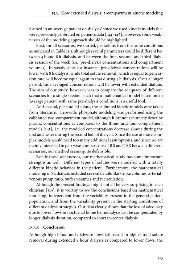
15.3. Slow extended dialysis: 2-compartment kinetic modeling
formed in an ‘average patient on dialysis’ since we used kinetic models thatwere previously calibrated on patient’s data [144–146]. However, someweak-nesses of the modeling approach should be highlighted.First, for all scenarios, we started, per solute, from the same conditions
as indicated in Table 15.3, although several parameters could be di�erent be-tween 4 h and 8 h dialysis, and between the �rst, second, and third dialy-sis session of the week (i.e. pre-dialysis concentrations and compartmentvolumes). In steady state, for instance, pre-dialysis concentrations will belower with 8 h dialysis, while total solute removal, which is equal to genera-tion rate, will become equal again to that during 4 h dialysis. Over a longerperiod, time averaged concentrations will be lower with extended dialysis.�e aim of our study, however, was to compare the adequacy of di�erentscenarios for a single session, such that a mathematical model based on an‘average patient’ with same pre-dialysis conditions is a useful tool.And second, per studied solute, the calibrated kineticmodels were taken
from literature. Herewith, phosphate modeling was performed using thecalibrated two-compartment model, although it cannot accurately describeplasma concentrations as compared to the three- and four-compartmentmodels [145], i.e. the modeled concentrations decrease slower during the�rst and faster during the second half of dialysis. Since the use of more com-plex models would need too many additional assumptions, and since we aremainly interested in pair wise comparisons of RR and TSR between di�erentscenarios, our method seems quite defensible.Beside these weaknesses, our mathematical study has some important
strengths as well. Di�erent types of solutes were modeled with a totallydi�erent kinetic behavior in the patient. Furthermore, the mathematicalmodeling of SL dialysis included several details like stroke volumes, arterial-venous pump ratio, bu�er volumes and recirculation.Although the present �ndings might not all be very surprising to each
clinician [319], it is worthy to see the conclusions based on mathematicalmodeling, independent from the variability present in the general patientpopulation, and from the variability present in the starting conditions ofdi�erent dialysis strategies. Our data clearly shows that the loss of adequacydue to lower �ows in nocturnal home hemodialysis can be compensated bylonger dialysis duration, compared to short in-center dialysis.
15.3.5 Conclusion
Although high blood and dialysate �ows still result in higher total soluteremoval during extended 8 hour dialysis as compared to lower �ows, the
213

15. Computational study on malfunctioning CVCs
gain is limited, especially for solutes with more complex compartment be-havior, such as β2M. Even when using a single lumen approach, total soluteremoval is superior in extended 8 h dialysis compared to standard 4 h dialy-sis. In view of the practical constraints of the home dialysis setting, low �owdialysis, even with single lumen approach, is a defensible option.
214

Six
General conclusions
215


Chapter
16Conclusions
�is is it. A�er 6 years of swimming, diving, �oating and sometimes evendrowning in the bio�uid site of vascular accesses (VA), you can �ndmy �nalconclusions herea�er. Since my PhD-work was built around the three typesof VA [arterio-venous �stula (AVF), arterio-venous gra� (AVG) and centralvenous catheter (CVC)], not one general but several research statements willbe discussed in the following section. While the di�erent studies in thisdissertation were grouped per VA type, the statements will be discussed perstudy method.
16.1 CFD analysis
�e main pressure drop in the AVF circuit should be over the anastomo-sis.
In general, there is a huge absence of interest in the geometry of the cre-ated arterio-venous anastomosis. �is can be noticed by the virtual totalabsence of studies regarding this topic, as well as by the lack of interest inthe geometry of the anastomosis in clinical studies dealing with AVF out-come. Creating a too small anastomosis reduces the chance of proper �s-tula maturation. But avoiding the non-maturation by creating a (too) largeanastomosis should not result in an increased prevalence of venous hyper-tension, cardiac overload, distal hypoperfusion or ischemia. We showed inour study on the impact of the anastomosis size (i.e. length and width) and
217

16. Conclusions
angle, that slightly changing the AVF anastomosis geometry has a large im-pact on the blood �ow and local pressure distribution, with a quadratic andcase-/patient-speci�c relation between �ow rate and pressure drop.During surgical creation of an AVF, as well as during complication solv-
ing interventions, should the anastomosis geometry be chosen with care,keeping in mind the impact of the geometry on pressure drop and �ow dis-tribution. �erefore, it can be stated that the main pressure drop in thearterio-venous circuit should be over the anastomosis to avoid complica-tions such as high pressure in the venous system, cardiac overload and distalischemia.
Using a helical pattern in the design of an AVG introduces a more com-plex �ow �eld and reduces, but does not delete, zones with unfavorablehemodynamic conditions.
To investigate the in�uence of helicity in the gra� design, a straight con-ventional gra� was compared to �ve di�erent helical designed gra�s. Weanalyzed the �ow �eld using di�erent wall shear stress descriptors as wellas the kinetic helicity in the bulk �ow and the pressure drop over the gra�section. �e investigated wall parameters (time-averaged wall shear stress,oscillatory shear index and relative residence time) can be linked to an in-creasing risk of intimal hyperplasia formation, thus stenosis formation.It is clear from our study, that introducing helicity in the design of an
AVG changes the downstream hemodynamics and introduces a more com-plex �ow �eld.�ere is however no trivial relationship between the numberof helical turns and the investigated wall shear parameters. Only the very‘swirling’ design, a pitch smaller than 6 times the gra� diameter, signi�cantlyreduces the area with unfavorable hemodynamic conditions at the venousanastomosis. However, in clinical practice, inserting this design under theskin of a patient will not be obvious. So, a design with a more modest he-licity pattern can be used to achieve more athero-protective conditions, butthe unfavorable hemodynamics will not be vanished. Furthermore, becauseevery gra� is, irrespective of the gra� design itself, subject to torsion andbending while connected in a loop con�guration between an artery and avein, gra�s should be studied case-by-case to qualify their ability to reduceunfavorable hemodynamics.
218

16.2. Experimental assessment
�e VectorFlow CVC outperforms standard catheters due to the negligi-ble recirculation.
We showed, based on kinetic modeling, that reversing the lines is a defen-sible practice to increase blood �ow in malfunctioning catheters. �e Vec-torFlow catheter, a double-D design with symmetrical tip, showed in a CFDanalysis, as well in an in vitro and in vivo investigation, a negligible recir-culation. Note that correct and reverse line connection are equal due to thesymmetrical design of the catheter tip. So from this point of view, the Vec-torFlow is a reliable option.
�e CFD analysis had the advantage that not only a global factor as re-circulation could be assessed, but a more in depth analysis could be per-formed as well. An ideal dialysis catheter, from a �uid-dynamic perspective,produces low shear stresses on the �uid, has a low percentage of prolongedblood residence time (cf. clotting) and maintains a low platelet lysis index(cf. hemolysis). �e mean shear stress and platelet lysis index were onlyslightly elevated (8% maximum) compared to reference case of a ‘shotgun’design, even with a signi�cant higher Reynolds number (18%) in the arterialand venous lumen.�e blood residence time was only modestly elevated.
�e symmetrical-tip design of theVectorFlow catheter introduces a neg-ligible recirculation and keeps the blood (�ow) parameters in a very accept-able range. However, additional pre-clinical data are required to con�rm theincreased catheter patency during long-term implantation.
16.2 Experimental assessment
�e pulse wave propagation model and the high �ow CFD solver, devel-oped in the ARCH-project, are experimentally validated and can be usedfor further clinical implementation.
For 1D-modeling, one cannot merely rely on patient data to determine whe-ther the physical descriptions in themodel are complete. Conducting an ex-perimental validation on an in vitro setup, with controllable andmeasurableboundary conditions (e.g. no vessel adaption), is probably the best option.For example, due to the inter-day variability of the patient’s blood pressure(i.e. by room temperature or the tranquility of the patient), an in vitro setupseems more ‘reliable’ when it comes to investigate the model’s fundamentalprinciples and the underlying physics. More over, compared to in vivo val-idation, in vitro validation is not hampered by the search for non-invasivemeasurement methods and by a limited number of accessible locations inthe circuit.
219

16. Conclusions
�e experimental validation of the pulsewave propagationmodel showedthat mean values of �ow and pressure can be predicted adequately, but thatviscoelasticity should be introduced in the model to match the diastole orsystole values.
�e pulse wave propagation model validation showed that calculatingthe pressure and �ow waves (with correct attenuation) is very challenging.�is knowledge makes it clear that studies relying on sensitive detection ofthe reduction or magni�cation of the pulse pressure, cannot just rely oncomputational modeling.For new CFD-codes, one can rely, in �rst instance, on the comparison
of the code against known benchmark results. However, to ensure that �owvs. pressure drop simulations, in challenging cases, give reliable results, invitro assessment seems still needed. Herewith, the overall �ow �eld is welldescribed by the solver and the pressure drop values are reliable up to aReynolds numbers of 2000. Hence, introducing a non-linear pressure losscoe�cient in the pulse wave propagationmodel, calculated by the CFD codeseems a good option to replace the pressure loss coe�cients based on e.g. T-shaped �ttings.
�e experimental validation of themodels’ fundamental principles opensthe way for further clinical implementation and in vivo validation.
Experimental lab work needs experienced researchers.
During the experiments in the context of in vitro validation, concerningthe pulse pressure analysis stenosis detection method and in the �eld ofneurosurgery [320, 321], much knowhow is gained on how in vitro �uid-mechanical experiments should be executed.As computers get faster and computational power increases (in 2006 the
Hydraulics lab had 3 single calculation computers, at present, a cluster ofover 200 cpus is available for the bioMMeda research group), the time con-suming experimental validation seems to vanish. But, still, in vitro valida-tion of numerical models is very valuable.In contrast to numerical investigations, constructing a large set of exper-
imental models and setups is not possible, while keeping cost, both moneyand time, within ‘budget’. One should, either investigate time to build upin-house knowledge on model construction or invest money in purchasinga state-of-the-art model.It was found in largemulticenter PIV-studies that �uctuations in the �ow
conditions and �uid properties need to be well controlled to increase accu-racy and reproducibility.We had the same experience when analyzing theresults of the preliminary PIV-study on a model of a kinked blood vessel
220

16.3. Diagnostic tools
[322, 323]. Herewith, we minimized, in our �nal PIV study, �uctuations onthe �ow conditions by installing a 1m long sti� tube proximal to the modelto obtain a symmetric in�ow and even checked the correctness of the as-sumed velocity pro�le. Furthermore, we closely monitored the �uid tem-perature and consequently adapted andmeasured the viscosity, to minimize�uid property �uctuations.To conclude, I want to point out that experimental work needs an ex-
perienced investigator. During the �rst construction of models and setups,a lack of skills may lead to leakages on multiple (unexpected) locations, airbubbles in the circuit, and in�ating and/or bursting silicon models (by mis-judgment of clamps or valves), such that pressure and �ow data will makecrazy antics. However, a�er obtained the necessary experience, collectingdata from a well controllable setup (as a validation for example), providesmost certainly a great sense of accomplishment.
16.3 Diagnostic tools
Pulsepressure analysis at the arterial needle canbeused todetect stenosesin early stage.
�e disadvantage of current stenoses detection methods, based on pressuredrop or �ow reduction, is the fact that they can only ‘trace’ stenoses with adiameter reduction of about 70% (≈90% area reduction).Our developed pulse pressure analysis (PPA) method, however, can de-
tect stenoses with a 50% and even a 25% diameter reduction.�is detectionin early stage can help the clinicians in the patient-speci�c �stula patencymanagement. �e PPA method is even independent of the �ow and heartrate.For use in clinical practice, the full pressure pro�le should be acquired
and analyzed.�is technique is feasible since most of the dialysis machinesnowadays have arterial line pressure sensors reportingmeanpressures. How-ever, a longitudinal study should reveal whether stenoses can be detected inearly stage only by, for example, weekly registration of the arterial needlepulse pressure.
Standard pulsed wave Doppler ultrasound measurements cannot pro-vide reliable blood �ow rates.
We performed a theoretical study based on patient-speci�c data, both preand post arterio-venous �stula creation, integrating computational �uid dy-namics calculations with an ultrasound simulator. We found that, when an-alyzing the simulated pulsed wave Doppler (PWD) spectrum in the brachial
221

16. Conclusions
and radial artery, the velocity component in the direction of the ultrasound(US) beam, in a centered, small, sample volume, can be captured accuratelyprovided that the velocity is derived using the mean of the pulsed waveDoppler spectrum rather than the outer envelope contour. However, whenderiving the �nal blood �ow rate based on these measurements, a high de-gree of inaccuracy occurs. We found that two factors induce this inaccuracy.First, the angle-correction of the velocity in the direction of the US-
beam towards the velocity in the longitudinal direction is largely in�uencedby the radial velocity components in the complex �ow �eld.Second, the largest error is introduced when the velocity in one point
(e.g. in the center of the vessel, 0D) has to be transferred to the cross-sectional mean velocity (2D) without any knowledge on the �ow pro�le: i.e.is the pro�le symmetrical, with its maximum velocity in the center and isthe shape of the pro�le parabolic, �at or something in between like Wom-ersley �ow? It cannot be predicted in advance, even not for the low �owpre-operative cases.In our study case, �ow at the brachial artery (pre- and postoperative) and
pre-operatively at the radial artery was best estimated assuming a parabolic�ow pro�le. For the post-operative radial artery acquisition, the most com-plex �ow pattern occurred and assuming a plug �ow pro�le resulted in thelowest bias.One might expect that the use of the larger sample volume (e.g. over the
full diameter of the vessel, 1D) should provide the most accurate estimate ofthe volume �ow (2D). Interestingly, our data indicated that this was not sys-tematically the case, probably because this method is challenged by the factthat velocities near the vessel wall are di�cult to measure, even in straightvessel segments.
16.4 Kinetic modeling
Reversing connection lines is the best alternative for dysfunctional dou-ble lumen CVCs during standard (4 h) dialysis.
In case of a dysfunctional double lumen CVC, two options can be taken: i.e.lowering blood �ow, or reversing the lines simultaneously and thereby in-creasing blood �ow. First, we found during an in vivo study, including 22patients, that reversing the lines in a well-functioning double lumen CVCdid not in�uence the solute removal of four generally studied solutes. Sincereversing the catheter linesmight increase recirculation (suction of cleansedblood back to the dialyzer) in a standard ‘shotgun’-type CVC, a mathemat-ical study, combining single pool modeling with a dialyzer model, was per-formed to determine dialysis adequacy based on urea removal. �e study222

16.4. Kinetic modeling
revealed that the total solute removal (TSR) of urea was only reduced by9.2% (at blood �ow rate, Qb, of 350ml/min) when the recirculation was be-low 10%.To better describe the retarded solute transport in the patient’s body, a
more complex 2-compartment kinetic model was combined with a dialyzermodel. Dialysis adequacy was checked for 4 di�erent solutes in 4 di�erentaccess types. We found a reduction of urea-TSR of only 3.3% when intro-ducing 10% recirculation (Qb 350ml/min). For a solute with a hamperedtransport within the patient (like β2M), an enormous recirculation of 47%only reduces solute removal with 5%.
�rough the 2-compartment kinetic modeling, we revealed that doublelumen reversed connection (introducing recirculation) with a high blood�ow rate, should be preferred above the correct line connection (negligi-ble recirculation) with a lowered �ow. Single lumen CVC dialysis seemed asuboptimal option in regular 4 h dialysis.
Low-�ow dialysis with double lumen CVC, or dialysis with single lumenCVC or single needle with an AVF, are considerable alternatives duringextended (8 h) dialysis.
Due to the available time during 8 h dialysis, solute kinetics in the patientplay an important role as compared to the dialyzer clearance. �erefore, 2-compartment kinetic modeling was performed for 4 solutes and 4 di�erentcases.We found the obvious fact that solute removal was higher when, for the
full length of the dialysis, a high �ow (as in regular dialysis) wasmaintained.However, solute removal with 8 h was not doubled compared to the 4 h dial-ysis (increase of 28-51%).One should keep in mind that when searching for the optimal parame-
ters for extended (nocturnal) dialysis, especially in the homecare setting, ex-tra boundary conditions play a role compared to a regular dialysis treatment(4 h in dialysis center). First, the quality of life is in�uenced by the patient’squality of sleep. �erefore avoiding the necessity of waking up during thenight to change concentrate bags, by reducing the blood and dialysate �owrate, is preferable.�is reduction in �ow rates also reduces the costs of water,which is in home-dialysis mostly covered by the patients themselves. Sincesolute removal in low �ow (175 instead of 350ml/min) dialysis is comparablewith that in regular daytime dialysis, low-�owdialysis is a worth consideringalternative.With a single lumen catheter, an increase in solute removal with 8 h dial-
ysis (13-35%) was present compared to the regular 4 h dialysis. Finally, with
223

16. Conclusions
a single needle punctured in an AVF, solute removal even increases a fewpercentages compared to the results for the single lumen CVC dialysis.�islast option was studied because in the homecare setting, patients o�en di-alyze (relying on their arterio-venous �stula as preferable vascular access)without assistance and a single needle puncturing might be preferable.�isbecause double needle puncturing is cumbersome and single needle punc-turing increases safety, due to a decreased frequency of line disconnection.�us, single needle/lumen hemodialysis seems to be the best option in thehome setting, keeping a good balance between dialysis adequacy, practicaluse, quality of life, and �nancial burden.
224

Bibliography
[1] E.N.Marieb andK.Hoehn.Anatomy&Physiology. PearsonBenjaminCumming, third edition, 2008.
[2] K. Van Canneyt and P. Verdonck. Comprehensive Biomedical Physics,Physical Medicine and Rehabilitation: Principles and Applications,chapter Mechanics of bio�uids in living body, pages –. Elsevier inc.,2013.
[3] D.E. Mohrman and L.J. Heller. Cardiovascular physiology. McGraw-Hill Professional, 2003.
[4] S. Eloot and P. Verdonck. Wiley Encyclopedia of Biomedical Engineer-ing, volume 6, chapter Modeling of transport phenomena in an arti-�cial kidney, pages AK1–AK24. John Wiley & Sons, Inc., 2006.
[5] A.S. Levey, K.-U. Eckardt, Y. Tsukamoto, A. Levin, J. Coresh,J. Rossert, D. De Zeeuw, T.H. Hostetter, N. Lameire, and G. Eknoyan.De�nition and classi�cation of chronic kidney disease: a position state-ment from Kidney Disease: Improving Global Outcomes (KDIGO).Kidney Int, 67(6):2089–2100, 2005.
[6] R.A. Hamer and A.M. El Nahas.�e burden of chronic kidney disease.BMJ, 332(7541):563–564, 2006.
[7] NKF-K/DOQI Clinical guidelines for chronic kidney disease: Evalua-tion, classi�cation, and strati�cation. Am J Kidney Dis, 39(1 Suppl1):S1–S266, 2002.
[8] M.K. Peck, N.Dusserre, K. Zagalski, S.A.Garrido,W.Wystrychowski,M.H. Glickman, N.A.F. Chronos, L. Cierpka, N. L’heureux, and T.N.McAllister. New biological solutions for hemodialysis access. J VascAccess, 12(3):185–192, 2011.
225

Bibliography
[9] N. Lameire, K. Jager,W. Van Biesen, D. de Bacquer, and R. Vanholder.Chronic kidney disease: A European perspective. Kidney Int, S99:S30–S38, 2005.
[10] A. Grassmann, S. Gioberge, S. Moeller, and G. Brown. ESRD Patientsin 2004: Global Overview of Patients Number, Treatment Modalitiesand Associated Trends. Nephrol Dial Transplant, 20:2587–2593, 2005.
[11] A. Grassmann, S. Gioberge, S. Moeller, and G. Brown. End-stage re-nal disease: global demographics in 2005 and observed trends. ArtifOrgans, 30(12):895–897, 2006.
[12] ERA-EDTA Registry Annual Report 2009. Technical report, ERA-EDTA Registry, Academic Medical Center, Department of MedicalInformatics, Amsterdam,�e Netherlands, 2011.
[13] Eurotransplant International Foundation Annual Report 2010. Tech-nical report, Eurotransplant International Foundation, 2011.
[14] Organ Procurement and Transplantation Network (OPTN) and Scien-ti�c Registry of Transplant Recipients (SRTR) 2010AnnualDataReport.Technical report, Department of Health and Human Services, HealthResources and Services Administration, Healthcare Systems Bureau,Division of Transplantation, Rockville, MD, US, 2011.
[15] K.S. Rabindranath, J. Adams, T.Z.Ali, A.M.MacLeod, L.Vale, J. Cody,S.A. Wallace, and C. Daly. Continuous ambulatory peritoneal dial-ysis versus automated peritoneal dialysis for end-stage renal disease.Cochrane Database Syst Rev, (2):CD006515, 2007.
[16] S. Eloot, W. Van Biesen, and R. Vanholder. Does the higher numberof dwells with APD result in better solute removal compared to CAPD.Int J Artif Organs, 33(7):484, 2010.
[17] USRDS 2010 Annual Data Report: Atlas of Chronic Kidney Disease andEnd-Stage Renal Disease in the United States. Technical report, Na-tional Institutes of Health, National Institute of Diabetes and Diges-tive and Kidney Diseases, 2010.
[18] J. Feehally, J. Floege, and R.J. Jonson. Comprehensive Clinical Nephrol-ogy. Mosby Elsevier, 2007.
[19] NKF-K/DOQI Clinical Practice Guidelines for Vascular Access: update2006. Am J Kidney Dis, 48(1 Suppl 1):S177–S322, 2006.
226

Bibliography
[20] J.J. Sands. Vascular access: the past, present and future. Blood Purif,27(1):22–27, 2009.
[21] M. Allon and M.L. Robbin. Increasing arteriovenous �stulas inhemodialysis patients: problems and solutions. Kidney Int, 62(4):1109–1124, 2002.
[22] J. Tordoir, B. Canaud, P. Haage, K. Konner, A. Basci, D. Fouque,J. Kooman, A. Martin-Malo, L. Pedrini, F. Pizzarelli, J. Tattersall,M. Vennegoor, C. Wanner, P. ter Wee, and R. Vanholder. EBPG onVascular Access. Nephrol Dial Transplant, 22 Suppl 2:ii88–i117, 2007.
[23] C.M. Kjellstrand. �e Achilles’ heel of the hemodialysis patient. ArchIntern Med, 138(7):1063–1064, 1978.
[24] A. Santoro, C. Canova, A. Freyrie, and E. Mancini. Vascular access forhemodialysis. J Nephrol, 19(3):259–264, 2006.
[25] J.H.M. Tordoir and V Mickley. European Guidelines for Vascular Ac-cess: Clinical Algorithms on Vascular Access for Hemodialysis. EDTNAERCA J, 29:131–136, 2003.
[26] J.H.M. Tordoir, P. Rooyens, R. Dammers, F.M. van der Sande,M. de Haan, and T.I. Yo. Prospective evaluation of failure modes inautogenous radiocephalic wrist access for hemodialysis. Nephrol DialTransplant 2003; 18:, .18:378–383, 2003.
[27] B.S. Dixon. Why don’t �stulas mature? Kidney Int, 70(8):1413–1422,2006.
[28] M.J. Brescia, J.E. Cimino, K. Appel, and B.F. Hurwich. ChronicHemodialysis Using Venipuncture and a Surgically Created Arteriove-nous Shunt. N Engl J Med, 275:1089–1092, 1966.
[29] J.E. Cimino.Historical Perspective onMore�an 60Years ofHemodial-ysis Access. Semin Vasc Surg, 20:136–140, 2007.
[30] M. Allon. Current management of vascular access. Clin J Am SocNephrol, 2(4):786–800, 2007.
[31] W.D. Paulson, Ram. S.J., and G.B. Zibari. Vascular Access: Anatomy,Examination, Managment. Sem Nephrol, 22(3):183–194, 2002.
227

Bibliography
[32] V.Wong, R. Ward, J. Taylor, S. Selvakumar, T. V. How, and A. Bakran.Factors associated with early failure of arteriovenous �stulae forhaemodialysis access. Eur J Vasc Endovasc Surg, 12(2):207–213, 1996.
[33] J. Tordoir. Commentary. Factors associated with early failure of arteri-ovenous �stulae for haemodialysis access. Eur J Vasc Endovasc Surg,42 Suppl 1:S55–S56, 2011.
[34] K. Van Canneyt, T. Pourchez, S. Eloot, C. Guillame, A. Bonnet,P. Segers, and P. Verdonck. Hemodynamic impact of anastomosis sizeand angle in side-to-end arteriovenous �stulae: a computer analysis. JVasc Access, 11(1):52–58, 2010.
[35] R.N. Planken. Hemodialysis vascular access imaging: Duplex ultra-sound and contrast-enhanced magnetic resonance angiography. PhDthesis, Universiteit Maastricht, 2007.
[36] T.C. Hodges, M.F. Fillinger, R.M. Zwolak, D.B. Walsh, F. Bech, andJ.L. Cronenwett. Longitudinal comparison of dialysis access methods:risk factors for failure. J Vasc Surg, 26(6):1009–1019, 1997.
[37] A. Falk. Maintenance and salvage of arteriovenous �stulas. J VascInterv Radiol, 17(5):807–813, 2006.
[38] K.M. Rigg. Dialysis access: Current Practice, chapter Complicationsof Vascular Access, pages 211–238. Imperial College Press, 2001.
[39] S.E. Wilson. Vascular Access Principles and Practice, chapter Autol-ogous Arteriovenous Fistulas: Direct Anastomosis for HemodialysisAccess, pages 82–100. Mosby, 2002.
[40] A. Asif. Vascular Access, chapter How can we make �stulae mature?,pages 29–34. Edizioni Minerva Medica, Turin, 2009.
[41] P. Roy-Chaudhury. Vascular Access, chapter Biological aspects of vas-cular access failure, pages 1–13. Edizioni Minerva Medica, Turin,2009.
[42] B. Ene-Iordache, L.Mosconi, L. Antiga, S. Bruno, A. Anghileri, G. Re-muzzi, and A. Remuzzi. Radial artery remodeling in response to shearstress increase within arteriovenous �stula for hemodialysis access. En-dothelium, 10(2):95–102, 2003.
228

Bibliography
[43] R. Baer, S. McDonald, R. Wu, and M. Mantha. Reversible advancedischemic hand atrophy due to arteriovenous �stula steal. Kidney Int,73(10):1203–1204, 2008.
[44] J.H. Tordoir, R. Dammers, and F.M. van der Sande. Upper extremityischemia and hemodialysis vascular access. Eur J Vasc Endovasc Surg,27(1):1–5, 2004.
[45] M. De Haan. Vascular Access, chapter Endovascular Treatment ofAngio-access induced upper extremity ischemia, pages 151–153. Edi-zioni Minerva Medica, Turin, 2009.
[46] H. Schanzer, M. Schwartz, E. Harrington, andM. Haimov. Treatmentof ischemia due to "steal" by arteriovenous �stula with distal artery lig-ation and revascularization. J Vasc Surg, 7(6):770–773, 1988.
[47] R.C. Knox, S.S. Berman, J.D. Hughes, A.T. Gentile, and J.L. Mills.Distal revascularization-interval ligation: a durable and e�ective treat-ment for ischemic steal syndrome a�er hemodialysis access. J Vasc Surg,36(2):250–5; discussion 256, 2002.
[48] C. Sessa, A. De Lambert, E. Cochet, O. Pichot, P. Palacin, and J.L.Magne. Vascular Access, chapter Ishemia and dril procedure, pages161–178. Edizioni Minerva Medica, Turin, 2009.
[49] J. Zanow, U. Kruger, and H. Scholz. Proximalization of the arterialin�ow: a new technique to treat access-related ischemia. J Vasc Surg,43(6):1216–21; discussion 1221, 2006.
[50] D.J. Minion, E. Moore, and E. Endean. Revision using distal in�ow: Anovel approach to dialysis-associated steal syndrome. Ann Vasc Surg,19(5):625–628, 2005.
[51] J. Zanow, K. Petzold, M. Petzold, U. Krueger, and H. Scholz. Flowreduction in high-�ow arteriovenous access using intraoperative �owmonitoring. J Vasc Surg, 44(6):1273–8, 2006.
[52] P.N. Suding and S.E. Wilson. Strategies for Management of IschemicSteal Syndrome. Semin Vasc Surg, 20:184–188, 2007.
[53] M. Sheltinga and F. Van Hoek. Vascular Access, chapter Banding forhigh �ow hemodialysis access, pages 141–150. EdizioniMinervaMed-ica, Turin, 2009.
229

Bibliography
[54] J.G. White, A. Kim, L.G. Josephs, and J.O. Menzoian. �e Hemody-namics of Steal Syndrome and Its Treatment. AnnVasc Surg, 13(3):308–312, 1999.
[55] V. Gambillara, G. Montorzi, C. Haziza-Pigeon, N. Stergiopulos, andP. Silacci. Arterial wall response to ex vivo exposure to oscillatory shearstress. J Vasc Res, 42(6):535–544, 2005.
[56] Bogdan Ene-Iordache and Andrea Remuzzi. Disturbed �ow in radial-cephalic arteriovenous �stulae for haemodialysis: low and oscillatingshear stress locates the sites of stenosis. Nephrol Dial Transplant,27(1):358–368, 2012.
[57] S. Sivanesan, T. How, and A. Bakran. Sites of Stenosis in AV Fistulaefor Haemodialysis access. Nephrol Dial Transplant, 14:118–120, 1999.
[58] L. Matyas, I. Mogan, A. Ebner, M. Lazarides, M. Mantell, R. Manson,E. Chemla, S. Mitra, M. Nikam, A. Tavakoli, and P. Roy-Chaudhury.Arteriovenous Anastomosis Creation using the Opti�ow AnastomoticConnector. J Vasc Access, 12(2):527–528, 2011.
[59] B.H. Scribner, R. Buri, J.E. Caner, R. Hegstrom, and J.M. Burnell.�etreatment of chronic uremia by means of intermittent hemodialysis: apreliminary report. Trans Am Soc Artif Intern Organs, 6:114–122,1960.
[60] I. Van Tricht, D. DeWachter, J. Tordoir, and P. Verdonck. Comparisonof the hemodynamics in 6mmand 4-7mmhemodialysis gra�s bymeansof CFD. J Biomech, 39(2):226–236, 2006.
[61] R. Dammers, R.N. Planken, K.P.M. Pouls, R.J. Van Det, H. Burger,F.M. Van Der Sande, and J.H.M. Tordoir. Evaluation of 4-mm to 7-mm versus 6-mm prosthetic brachial-antecubital forearm loop accessfor hemodialysis: results of a randomized multicenter clinical trial. JVasc Surg, 37(1):143–148, 2003.
[62] D.E. Finlay, D.G. Longley, M.C. Foshager, and J.G. Letourneau. Du-plex and color Doppler sonography of hemodialysis arteriovenous �stu-las and gra�s. Radiographics, 13(5):983–989, 1993.
[63] C.J. Chang, P.J. Ko, L.A. Hsu, Y.S. Ko, Y.L Ko, C.F. Chen, C.C. Huang,T.S. Hsu, Y.S. Lee, and J.H.S. Pang. Highly increased cell prolifera-tion activity in the restenotic hemodialysis vascular access a�er percuta-neous transluminal angioplasty: implication in prevention of restenosis.Am J Kidney Dis, 43(1):74–84, 2004.
230

Bibliography
[64] F.P. Christidou, V.I. Kalpakidis, K.D. Iatrou, I.A. Zervidis, G.I.Bamichas, L.C. Gionanlis, T.A. Natse, and K.J. Sombolos. Per-cutaneous transluminal angioplasty (PTA) and venous stenting inhemodialysis patients with vascular access-related venous stenosis orocclusion. Radiographiy, 12:127–133, 2006.
[65] L. Soletti, Y. Hong, J. Guan, J.J. Stankus, M.S. El-Kurdi, W.R. Wagner,and D.A. Vorp. A bilayered elastomeric sca�old for tissue engineeringof small diameter vascular gra�s. Acta Biomater, 6(1):110–122, 2010.
[66] O. Sakai, K. Kanda, H. Ishibashi-Ueda, K. Takamizawa, A. Ametani,H. Yaku, and Y. Nakayama. Development of the wing-attached rod foracceleration of "Biotube" vascular gra�s fabrication in vivo. J BiomedMater Res B Appl Biomater, 83(1):240–247, 2007.
[67] M. Lei, J. P. Archie, and C. Kleinstreuer. Computational design of abypass gra� that minimizes wall shear stress gradients in the region ofthe distal anastomosis. J Vasc Surg, 25(4):637–646, 1997.
[68] A.J. Sorom, Christopher B. Hughes, J.T. McCarthy, B.M. Jenson,M. Prieto, J.M. Panneton, S. Sterio�, M.D. Stegall, and S.L. Nyberg.Prospective, randomized evaluation of a cu�ed expanded polytetra�u-oroethylene gra� for hemodialysis vascular access. Surgery, 132(2):135–140, 2002.
[69] Y.-H. Liu, Y.-N. Hung, H.-C. Hsieh, and P.-J. Ko. Impact of cu�ed,expanded polytetra�uoroethylene dialysis gra�s on gra� outlet stenosis.World J Surg, 30(12):2290–2294, 2006.
[70] C.G. Caro, N.V. Watkins, and S.J. Sherwin. Helical gra�. Patent. US2007/0021707 A1, 2007.
[71] S.J. Sherwin, O. Shah, D.J. Doorly, J. PeirÃş, Y. Papaharilaou,N. Watkins, C.G. Caro, and C.L. Dumoulin. �e in�uence of out-of-plane geometry on the �ow within a distal end-to-side anastomosis. JBiomech Eng, 122(1):86–95, 2000.
[72] Y. Papaharilaou, D. J. Doorly, and S. J. Sherwin. �e in�uence of out-of-plane geometry on pulsatile �ow within a distal end-to-side anasto-mosis. J Biomech, 35(9):1225–1239, 2002.
[73] G. Coppola and C. Caro. Arterial geometry, �ow pattern, wall shearand mass transport: potential physiological signi�cance. J R Soc Inter-face, 6(35):519–528, 2009.
231

Bibliography
[74] C.G. Caro, N.J. Cheshire, and N. Watkins. Preliminary comparativestudy of small amplitude helical and conventional ePTFE arteriovenousshunts in pigs. J R Soc Interface, 2(3):261–266, 2005.
[75] F. Loth, P.F. Fischer, and H.S. Bassiouny. Blood �ow in end-to-sideanastomoses. Annu Rev Fluid Mech, 40:367–393, 2008.
[76] H.J.T.A.M. Huijbregts, P.J. Blankestijn, C.G. Caro, N.J.W. Cheshire,M.T.C. Hoedt, R.P. Tutein Nolthenius, and F.L. Moll. A helical PTFEarteriovenous access gra� to swirl �ow across the distal anastomosis:results of a preliminary clinical study. Eur J Vasc Endovasc Surg,33(4):472–475, 2007.
[77] M. Glickman. Vascular Access, chapter New Advancements in pros-thetic gra�s for hemodialysis, pages 95–98. EdizioniMinervaMedica,2009.
[78] A. Krueger, U.and Huhle, K. Krys, and H. Scholz. E�ect of taperedgra�s on hemodynamics and �ow rate in dialysis access gra�s. ArtifOrgans, 28(7):623–628, 2004.
[79] S. Shaldon, L. Chiandussi, and B. Higgs. Heaemodialysis by percu-taneous catheterization of the femoral artery and vain with regionalheparinization. Lancet, II:857–859, 1961.
[80] L. Kamper and M. Hofer. �e Chest X-Ray: A Systematic TeachingAtlas, chapter Foreign Bodies, pages 157–182. Georg�ieme Verlag,2007.
[81] K. Konner. History of vascular access for haemodialysis. Nephrol DialTransplant, 20(12):2629–2635, 2005.
[82] J. Erben, J. Kvasnicaka, J. Bastecky, andV. Vortel. Experience with rou-tine use of subclavian vein cannulation in heemodialysis. Proc EDTA,6:59–64, 1969.
[83] F. Schillinger, D. Schillinger, R. Montagnac, and T. Milcent. Postcatheterisation vein stenosis in haemodialysis: comparative angio-graphic study of 50 subclavian and 50 internal jugular accesses.NephrolDial Transplant, 6(10):722–724, 1991.
[84] Z.J. Twardowski. Advantages and limits of the jugular catheter ap-proach. Nephrol Dial Transplant, 10(12):2178–2182, 1995.
232

Bibliography
[85] W. Develter, A. De Cubber, W. Van Biesen, R. Vanholder, andN. Lameire. Survival and complications of indwelling venous cathetersfor permanent use in hemodialysis patients. Artif Organs, 29(5):399–405, 2005.
[86] R. Schindler. Vascular Access, chapter Catheter implantation andcomplications, pages 71–74. Edizioni Minerva Medica, Turin, 2009.
[87] Rhode Island Vascular Institute (RIVI).http://www.rivascularinstitute.com/images/da2.jpg, 2012.
[88] J.A. Akoh. Dialysis access: Current Practice, chapter Central venouscatheters, pages 257–302. Imperial College Press, 2001.
[89] M.G. Tal, A.J. Peixoto, S.T. Crowley, N. Denbow, D. Eliseo, and J. Pol-lak. Comparison of side hole versus non side hole high �owhemodialysiscatheters. Hemodial Int, 10(1):63–67, 2006.
[90] H.-D. Polaschegg and C. Shah. Overspill of catheter locking solution:safety and e�cacy aspects. ASAIO J, 49(6):713–715, 2003.
[91] M. Vorweg, E. Monaca, M. Doehn, and F. Wappler. �e ’heparinlock’: cause for iatrogenic coagulopathy. Eur J Anaesthesiol, 23(1):50–53, 2006.
[92] M. Agharazii, I. Plamondon, M. Lebel, P. Douville, and S. Desmeules.Estimation of heparin leak into the systemic circulation a�er centralvenous catheter heparin lock. Nephrol Dial Transplant, 20(6):1238–1240, 2005.
[93] S. Ruesch, B. Walder, and M.R. TramÃĺr. Complications of centralvenous catheters: internal jugular versus subclavian access–a systematicreview. Crit Care Med, 30(2):454–460, 2002.
[94] S.R. Ash. Fluid mechanics and clinical success of central venouscatheters for dialysis–answers to simple but persisting problems. SeminDial, 20(3):237–256, 2007.
[95] H.L. Moore. Side holes at the tip of chronic hemodialysis catheters areharmful. J Vasc Access, 2(1):8–16, 2001.
[96] F. Tesio, H. De Baz, G. Panarello, G. Calianno, P. Quaia, A. Raimondi,and D. Schinella. Double catheterization of the internal jugular veinfor hemodialysis: indications, techniques, and clinical results. Artif Or-gans, 18(4):301–304, 1994.
233

Bibliography
[97] B. Canaud, H. Leray-Moragues, V. Garrigues, and C. Mion. Perma-nent twin catheter: a vascular access option of choice for haemodialysisin elderly patients. Nephrol Dial Transplant, 13 Suppl 7:82–88, 1998.
[98] G. Mareels, R. Kaminsky, S. Eloot, and P.R. Verdonck. Particle imagevelocimetry-validated, computational �uid dynamics-based design toreduce shear stress and residence time in central venous hemodialysiscatheters. ASAIO J, 53(4):438–446, 2007.
[99] M.G. Tal. Comparison of recirculation percentage of the palindromecatheter and standard hemodialysis catheters in a swine model. J VascInterv Radiol, 16(9):1237–1240, 2005.
[100] R.A. Mankus, S.R. Ash, and J.M. Sutton. Comparison of blood �owrates and hydraulic resistance between theMahurkar catheter, the Tesiotwin catheter, and the Ash Split Cath. ASAIO J, 44(5):M532–M534,1998.
[101] S.R. Ash. Advances in tunneled central venous catheters for dialysis:design and performance. Semin Dial, 21(6):504–515, 2008.
[102] H.E. Katzman, R.B. McLa�erty, J.R. Ross, M.H. Glickman, E.K. Pe-den, and J.H. Lawson. Initial experience and outcome of a newhemodialysis access device for catheter-dependent patients. J Vasc Surg,50(3):600–7, 607.e1, 2009.
[103] R.L. Pisoni, E.W. Young, D.M. Dykstra, R.N. Greenwood, E. Hecking,B. Gillespie, R.A. Wolfe, D.A. Goodkin, and P.J. Held. Vascular accessuse and outcomes: results from the DOPPS. Kidney Int, 137:305–316,2002.
[104] National Vascular Access Improvement Initiative: Fistula First Break-through Initiative FFBI. http://www.�stula�rst.org/, 2012.
[105] A.N. Sidawy, R. Gray, A. Besarab, M. Henry, E. Ascher, M. Silva Jr,A. Miller, L. Scher, S. Trerotola, R.T. Gregory, R.B. Rutherford, andK.C. Kent. Recommended standards for reports dealing with arteriove-nous hemodialysis accesses. J Vasc Surg, 35(3):603–610, 2002.
[106] H.J.T. Huijbregts, M.L. Bots, C.H.A.Wittens, Y.C. Schrama, F.L. Moll,P.J. Blankestijn, and C.I.M.I.N.O study group. Hemodialysis arteri-ovenous �stula patency revisited: results of a prospective, multicenterinitiative. Clin J Am Soc Nephrol, 3(3):714–719, 2008.
234

Bibliography
[107] M.J. Oliver, R.L. McCann, O.S. Indridason, D.W. Butterly, and S.J.Schwab. Comparison of transposed brachiobasilic �stulas to upper armgra�s and brachiocephalic �stulas. Kidney Int, 60(4):1532–1539, 2001.
[108] K. McLaughlin, B. Jones, R. Mactier, and C. Porteus. Long-term vas-cular access for hemodialysis using silicon dual-lumen catheters withguidewire replacement of catheters for technique salvage. Am J KidneyDis, 29(4):553–559, 1997.
[109] J.L. Xue, D. Dahl, J. P. Ebben, andA.J. Collins.�e association of initialhemodialysis access type with mortality outcomes in elderly MedicareESRD patients. Am J Kidney Dis, 42(5):1013–1019, 2003.
[110] S. Pastan, J.M. Soucie, and W.M. McClellan. Vascular access andincreased risk of death among hemodialysis patients. Kidney Int,62(2):620–626, 2002.
[111] M. Allon, J. Daugirdas, T.A. Depner, T. Greene, D. Ornt, and S.J.Schwab. E�ect of change in vascular access on patient mortality inhemodialysis patients. Am J Kidney Dis, 47(3):469–477, 2006.
[112] H.C. Rayner, R.L. Pisoni, B.W. Gillespie, D.A. Goodkin, T. Akiba,T. Akizawa, A. Saito, E.W. Young, F.K. Port, Dialysis Outcomes , andPractice Patterns Study. Creation, cannulation and survival of arte-riovenous �stulae: data from the Dialysis Outcomes and Practice Pat-terns Study. Kidney Int, 63(1):323–330, 2003.
[113] R.L. Anel, A.S. Yevzlin, and P. Ivanovich. Vascular access and patientoutcomes in hemodialysis: questions answered in recent literature. ArtifOrgans, 27(3):237–241, 2003.
[114] A. Bode, A. Caroli, W. Huberts, N. Planken, L. Antiga, M. Bosboom,A. Remuzzi, J. Tordoir, and ARCH project consortium . Clinicalstudy protocol for the ARCH project - computational modeling for im-provement of outcome a�er vascular access creation. J Vasc Access,12(4):369–376, 2011.
[115] W. Huberts. Personalized computational modeling of vascular accesscreation. PhD thesis, Universiteit Maastricht, 2012.
[116] A.C. Guyton. Textbook ofMedical Physiology. Saunders, Philadelphia,2nd edition, 1961.
235

Bibliography
[117] L.F.Mockros andR. Leonard. Compact cross-�ow tubular oxygenators.Trans Am Soc Artif Intern Organs, 31:628–33, 1985.
[118] D. Quemada. A rheological model for studying the hematocrit de-pendence of red cell-red cell and red cell-protein interactions in blood.Biorheology, 18(3-6):501–516, 1981.
[119] G. Cockelet. Handbook of Bioengineering, chapter�e rheology andtube �ow of blood, pages 14.11–14.17. McGraw-Hill Book Company,1986.
[120] R. Berguer andN.H.C.Hwang. Critical Arterial Stenosis: A�eoreticaland Experimental Solution. Ann. Surg., 180:39–50, 1974.
[121] L. Antiga and D.A. Steinman. Rethinking turbulence in blood. Biorhe-ology, 46(2):77–81, 2009.
[122] A.M. Malek, S.L. Alper, and S. Izumo. Hemodynamic shear stress andits role in atherosclerosis. JAMA, 282(21):2035–2042, 1999.
[123] D.N. Ku, D.P. Giddens, C.K. Zarins, and S. Glagov. Pulsatile �ow andatherosclerosis in the human carotid bifurcation. Positive correlation be-tween plaque location and low oscillating shear stress. Arteriosclerosis,5(3):293–302, 1985.
[124] H.A. Himburg, D.M. Grzybowski, A.L. Hazel, J.A. LaMack, X.M. Li,and M.H. Friedman. Spatial comparison between wall shear stressmeasures and porcine arterial endothelial permeability. Am J PhysiolHeart Circ Physiol, 286(5):H1916–H1922, 2004.
[125] S.-W. Lee, L. Antiga, and D.A. Steinman. Correlations among indica-tors of disturbed �ow at the normal carotid bifurcation. J Biomech Eng,131(6):061013, 2009.
[126] A. Belian, O. Chkhetiani, E. Golbraikh, and S.Moiseev. Helical turbu-lence: turbulent viscosity and instability of the second moments. Phys-ica A, 258(1-2):55–68, 1998.
[127] M. Grigioni, C. Daniele, U. Morbiducci, C. Del Gaudio, G. D’Avenio,A. Balducci, and V. Barbaro. Proposal for a quantitative description ofblood spiral �ow in medical devices. Int J Artif Organs, 27(3):231–242,2004.
236

Bibliography
[128] M. Grigioni, C. Daniele, U. Morbiducci, C. Del Gaudio, G. D’Avenio,A. Balducci, and V. Barbaro. A mathematical description of blood spi-ral �ow in vessels: application to a numerical study of �ow in arterialbending. J Biomech, 38(7):1375–1386, 2005.
[129] R. Kaminsky. Particle Image Velocimetry Analysis of the Blood Flow inCardiovascular Devices. PhD thesis, Ghent University, 2007.
[130] I. Khodarahmi, M. Shakeri, M. Sharp, and A.A. Amini. Using PIVto determine relative pressures in a stenotic phantom under steady �owbased on the pressure-poisson equation. Conf Proc IEEE EngMed BiolSoc, 2010:2594–2597, 2010.
[131] Y. Hoi, S.H. Woodward, M. Kim, D.B. Taulbee, and H. Meng. Val-idation of CFD simulations of cerebral aneurysms with implication ofgeometric variations. J Biomech Eng, 128(6):844–851, 2006.
[132] S.W.Day and J.C.McDaniel. PIVmeasurements of �ow in a centrifugalblood pump: time-varying �ow. J Biomech Eng, 127(2):254–263, 2005.
[133] S.W.Day and J.C.McDaniel. PIVmeasurements of �ow in a centrifugalblood pump: steady �ow. J Biomech Eng, 127(2):244–253, 2005.
[134] R.B. Medvitz, V. Reddy, S. Deutsch, K.B. Manning, and E.G. Pater-son. Validation of a CFDmethodology for positive displacement LVADanalysis using PIV data. J Biomech Eng, 131(11):111009, 2009.
[135] G.A. Giridharan, C. Lederer, A. Berthe, L. Goubergrits, J. Hutzenlaub,M.S. Slaughter, R.D. Dowling, P.A. Spence, and S.C. Koenig. Flowdynamics of a novel counterpulsation device characterized by CFD andPIV modeling. Med Eng Phys, 33(10):1193–1202, 2011.
[136] J. Charonko, S. Karri, J. Schmieg, S. Prabhu, and P. Vlachos. In vitro,time-resolved PIV comparison of the e�ect of stent design on wall shearstress. Ann Biomed Eng, 37(7):1310–1321, 2009.
[137] R. Kaminsky, K. Dumont, H.Weber,M. Schroll, and P. Verdonck. PIVvalidation of blood-heart valve lea�et interaction modelling. Int J ArtifOrgans, 30(7):640–648, 2007.
[138] R. Kaminsky, U. Morbiducci, M. Rossi, L. Scalise, P. Verdonck, andM. Grigioni. Time-resolved PIV technique for high temporal resolutionmeasurement of mechanical prosthetic aortic valve �uid dynamics. IntJ Artif Organs, 30(2):153–162, 2007.
237

Bibliography
[139] K.B. Manning, V. Kini, A.A. Fontaine, S. Deutsch, and J.M. Tarbell.Regurgitant �ow �eld characteristics of the St. Jude bilea�et mechan-ical heart valve under physiologic pulsatile �ow using particle imagevelocimetry. Artif Organs, 27(9):840–846, 2003.
[140] M.D. Ford, H.N. Nikolov, J.S. Milner, S.P. Lownie, E.M. Demont,W. Kalata, F. Loth, D.W. Holdsworth, and D.A. Steinman. PIV-measured versus CFD-predicted �ow dynamics in anatomically realisticcerebral aneurysm models. J Biomech Eng, 130(2):021015, 2008.
[141] S.C.P. Cheung, K.K.L. Wong, G.H. Yeoh, W. Yang, R. Tu, J.and Beare,and T. Phan. Experimental and numerical study on the hemodynamicsof stenosed carotid bifurcation. Australas Phys Eng SciMed, 33(4):319–328, 2010.
[142] K. Stanislas, K. Okamoto, C.J. Kahler, J. Westerweel, and F. Scarano.Main Results of the�ird International Challenge. Exp. Fluids, 45:27–71, 2008.
[143] P. Hariharan, M. Giarra, V. Reddy, S.W. Day, K.B. Manning,S. Deutsch, S.F.C. Stewart, M.R.Myers, M.R. Berman, G.W. Burgreen,E.G. Paterson, and R.A. Malinauskas. Multilaboratory particle imagevelocimetry analysis of the FDA benchmark nozzle model to supportvalidation of computational �uid dynamics simulations. J BiomechEng, 133(4):041002, 2011.
[144] S. Stiller, X. Q. Xu, N. Gruner, J. Vienken, and H. Mann. Validationof a two-pool model for the kinetics of beta2-microglobulin. Int J ArtifOrgans, 25(5):411–420, 2002.
[145] E.M. Spalding, P.W. Chamney, and K. Farrington. Phosphate kinet-ics during hemodialysis: Evidence for biphasic regulation. Kidney Int,61(2):655–667, 2002.
[146] S. Eloot, A. Torremans, R. De Smet, B. Marescau, D. DeWachter, P.P.DeDeyn, N. Lameire, P.Verdonck, andR.Vanholder. Kinetic behaviorof urea is di�erent from that of other water-soluble compounds: the caseof the guanidino compounds. Kidney Int, 67(4):1566–1575, 2005.
[147] U. Krueger, J. Zanow, and H. Scholz. Computational Fluid Mechanicsand Vascular Access. Art Org, 26(7):571–575, 2002.
238

Bibliography
[148] Z. Kharboutly, M. Fenech, J.M. Treutenaere, I. Claude, and C. Legal-lais. Investigations into the relationship between hemodynamics andvascular alterations in an established arteriovenous �stula. Med EngPhys, 29:999–1007, 2007.
[149] S. Sivanesan, T.V. How, R.A. Black, and A. Bakran. Flow patterns inthe radiocephalic arteriovenous �stula: an in vitro study. J Biomech,32:915–925, 1999.
[150] J.R. Welty, C.E. Wicks, S.E. Wilson, and G. Rorrer. Fundamentals ofMomentum, Heat and Mass Transfer. John Wiley & Sons Inc., NewYork, 4th edition, 2001.
[151] A.E. Hendriksson and D. Bergqvist. Steal syndrome of the hemodial-ysis vascular access: Diagnosis and treatment. J Vasc Access, 5:62–68,2004.
[152] P. Bachleda, P. Utikal, Z. Kojecky, P. Drac, M. KÃČÂűcher, M. Cerna,and J. Zadrazil. Autogenous Arteriovenous Elbow Fistula ForHaemodialysis and Upper Extremity Ischemia. Biomed Pap Med FacUniv Palacky Olomouc Czech Repub, 151(1):129–132, 2007.
[153] R.W. Barnes. Hemodynamics for the Vascular Surgeon. Arch Surg,115:216–223, 1980.
[154] C.L. Wixon, J.D. Hughes, and J.L. Mills. Understanding Strategies forthe Treatment of Ischemic Steal Syndrome a�er Hemodialysis Access. JAm Coll Surg, 191(3):301–310, 2000.
[155] C.B. Anderson, E.E. Etheredge, H.R. Harter, R.J. Gra�, J.E. Codd, andW.T. Newton. Local Blood Flow Characteristics of Arteriovenous Fis-tulas in the Forearm for Dialysis. Surg Gynec Obst, 144(4):531–533,1977.
[156] Y. Pousset, P. Lermusiaux, G. Berton, J. Le Gouez, and R. Leroy. Flowdynamics through end-to-side anastomosis. AnnVasc Surg, 20(6):774–779, 2006.
[157] L.P. Chua, W. Ji, and T. Zhou. In vitro study on the steady �ow char-acteristics of proximal anastomotic models. Int Commun Heat Mass,32:464–472, 2005.
239

Bibliography
[158] N.H. Staalsen, M. Ulrich, J. Winther, E.M. Pederson, T. How, andH.Nygaard.�e anastomosis angle does change the �ow �elds at vascu-lar end-to-side anastomoses in vivo. J Vasc Surg, 21(3):460–471, 1995.
[159] C. Leon and A. Asif. Arteriovenous access and hand pain: the distalhypoperfusion ischemic syndrome. Clin JAmSocNephrol, 2(1):175–83,2007.
[160] J. Malik, V. Tuka, Z. Kasalova, E. Chytilova, M. Slavikova, P. Clagett,I. Davidson, B. Dolmatch, D. Nichols, andM.Gallieni. Understandingthe dialysis access steal syndrome. A review of the etiologies, diagnosis,prevention and treatment strategies. J Vasc Access, 9(3):155–66, 2008.
[161] H. Schanzer and D. Eisenberg. Management of steal syndrome result-ing from dialysis access. Semin Vasc Surg, 17(1):45–9, 2004.
[162] K. Konner. A primer on the AV �stula - Achilles’ heel, but also Cin-derella of haemodialysis. Nephrol Dial Transplant, 14(9):2094–2098,1999.
[163] R. Dammers. Non-invasive Assessment of Arterial Remodeling in Ar-teriovenous Fistulas for Hemodialysis. PhD thesis, University ofMaas-tricht,�e Netherlands, 2003.
[164] E. Wijnen, X.H.A. Keuter, R.N. Planken, F.M. van der Sande, TordoirJ.H.M., K.M. Leunissen, and J.P. Kooman.�e relation between vascu-lar access �ow and di�erent types of vascular access with systemic hemo-dynamics in hemodialysis patients. Arti�cial Organs, 29(12):960–964,2005.
[165] M.L. Robbin, N.E. Chamberlain, M.E. Lockhart, M.H. Gallichio, C.J.Young, M.H. Deierhoi, andM. Allon. Hemodialysis arteriovenous �s-tula maturity: US evaluation. Radiology, 225:59–64, 2002.
[166] A. Bakran, V. Mickley, and J. Passlick-Deetjen, editors. Manage-ment of the Renal Patient: Clinical Algorithms on Vascular Accessfor Haemodialysis. Pabst Science Publishers, D-49525 Lengerich,Deutschland, 2003. ISBN 978-3-936142-86-0.
[167] D. Shemesh, I. Goldin, D. Berelowitz, I. Zaghal, C. Zigelman, andO. Olsha. Blood Flow Volume Changes in the Maturing ArteriovenousFistula for Hemodialysis. Ultrasound inMed Biol, 33(5):727–733, 2007.
240

Bibliography
[168] W. Huberts, A.S. Bode, W. Kroon, R.N. Planken, J.H.M. Tordoir, F.N.van de Vosse, and E.M.H. Bosboom. A pulse wave propagation modelto support decision-making in vascular access planning in the clinic.Med Eng Phys, 34(2):233–248, 2012.
[169] P. Reymond, Y. Bohraus, F. Perren, F. Lazeyras, and N. Stergiopulos.Validation of a patient-speci�c one-dimensional model of the systemicarterial tree. Am J Physiol Heart Circ Physiol, 301(3):H1173–H1182,2011.
[170] K.S. Matthys, J. Alastrueya, J. Peiro, A.W. Khir, P. Segers, P.R. Ver-donck, K.M. Parker, and S.J. Sherwin. Pulse wave propagation ina model human arterial network: Assessment of 1-D numerical sim-ulations against in vitro measurements. Journal of Biomechanics,40:3476–3486, 2007.
[171] P. Reymond, F.Merenda, F. Perren, D. Rüfenacht, andN. Stergiopulos.Validation of a one-dimensional model of the systemic arterial tree. AmJ Physiol Heart Circ Physiol, 297:208–222, 2009.
[172] D. Bessems, C.G. Giannopapa, M.C.M. Rutten, and van de Vosse F.N.Experimental Validation of a Time-domain-based Wave PropagationModel of Blood Flow in Viscoelastic Vessels. J Biomech, 41:284–91,2008.
[173] A. Swillens, L. Lanoye, J. De Backer, N. Stergiopulos, P.R. Verdonck,F. Vermassen, and S. Segers. E�ect of an Abdominal Aortic Aneurysmon Wave Re�ection in the Aorta. IEEE Transactions on biomedicalengineering, 55(5):1602–1611, 2008.
[174] D. Xiu and S.J. Sherwin. Parametric uncertainty analysis of pulse wavepropagation in a model of a human arterial network. J Comp Phys,226:1385–1407, 2007.
[175] C.P. Robert and G.C. Casella. Monte Carlo statistical methods.Springer, New York, 2000.
[176] K.VanCanneyt, RN. Planken, S. Eloot, P. Segers, andP.Verdonck. Ex-perimental study of a new method for early detection of vascular accessstenoses: pulse pressure analysis at hemodialysis needle. Artif Organs,34(2):113–117, 2010.
241

Bibliography
[177] M. in ’t Veer, M.C.F. Geven, M.C.M. Rutten, A. van der Horst, W.H.Aarnoudse, N.H.J. Pijls, and F.N. van de Vosse. Continuous infusionthermodilution for assessment of coronary �ow: theoretical backgroundand in vitro validation. Med Eng Phys, 31(6):688–694, 2009.
[178] B.W.A.M.M. Beulen, N. Bijnens, G.G. Koutsouridis, P.J. Brands,M.C.M. Rutten, and F.N. van de Vosse. Toward noninvasive bloodpressure assessment in arteries by using ultrasound. Ultrasound inMedBiol, 37(5):788–797, 2011.
[179] A.C. Guyton and J.E. Hall. Textbook of medical physiology. W.B. Saun-ders Company, 1996.
[180] A. Gardel. Pressure Drops in Flows�rough T-shaped Fittings. BulletinTechnique de la Suisse Romande, 9:123–130, 1957.
[181] A. Gardel. Pressure Drops�rough T-shaped Fittings. Bulletin Tech-nique De La Suisse Romande, 10:143–148, 1957.
[182] N.Westerhof, G. Elzinga, andP. Sipkema. AnArti�cial Arterial Systemfor Pumping Hearts. J Appl Phys, 31(5):776–781, 1971.
[183] N. Stergiopulos, J.J. Meister, and N.Westerhof. Evaluation of Methodsfor Estimation of Total Arterial Compliance. Am J Physiol, 268:H1540–H1548, 1995.
[184] M.D. McKay, R.J. Beckman, andW.J. Conover. A comparison of threemethods for selecting values of input variables in the analysis of outputfrom a computer code. Technometrics, 21:239–245, 1979.
[185] W. Huberts, C. de Jonge, W.P.M. van der Linden, M.A. Inda, J.H.M.Tordoir, F.N. van de Vosse, and E.M.H. Bosboom. A sensitivity analy-sis to improve the measurement protocol to assess parameters for a per-sonalized wave propagation model: application to AVF surgery. Sub-mitted to Med Eng Phys, 2011.
[186] J. Alastruey, A.W. Khir, K.S. Matthys, P. Segers, S.J. Sherwin, P.R. Ver-donck, K.H. Parker, and J. Peiró. Pulse wave propagation in a modelhuman arterial network: Assessment of 1-D visco-elastic simulationsagainst in vitro measurements. J Biomech, 44:2250–2258, 2011.
[187] D.E. Strandness andD.S. Sumner. Hemodynamics for surgeons. Gruneand Stratton, New York, 1975.
242

Bibliography
[188] W.W. Nichols and M.F. O’Rourke. McDonalds’s blood �ow in arter-ies : theoretical, experimental and clinical principles. Edward Arnold,London, 1998.
[189] R. Raghu, I. E. Vignon-Clementel, C. A. Figueroa, and C.A. Taylor.Comparative study of viscoelastic arterial wall models in nonlinear one-dimensional �nite element simulations of blood �ow. J Biomech Eng,133(8):081003, 2011.
[190] B.N. Steele, D. Valdez-Jasso, M.A. Haider, and M.S. Olufsen. Pre-dicting arterial �ow and pressure dynamics using a 1D �uid dynamicsmodel with a viscoelastic wall. Siam JApplMath, 71 (4):1123–1143, 2011.
[191] B. Learoyd andM. Taylor. Alterations with age in the viscoelastic prop-erties of human arterial walls. Clinical Research, 18:278–292, 1966.
[192] T. Imura, K. Yamamoto, T. Satoh, K. Kanamori, T.Mikami, andH. Ya-suda. In vivo viscoelastic behavior in the human aorta. CirculationResearch, 66:1413–1419, 1990.
[193] L. Botti and D.A. Di Pietro. A pressure-correction scheme forconvection-dominated incompressible �ows with discontinuous velocityand continuous pressure. J. Comput. Phys., 230:572–585, 2011.
[194] Z. Kharboutly, V. Deplano, E. Bertrand, and C. Legallais. Numericaland experimental study of blood �ow through a patient-speci�c arte-riovenous �stula used for hemodialysis. Med Eng Phys, 32(2):111–118,2010.
[195] F. Loth, P.F. Fischer, N. Arslan, C.D. Bertram, S.E. Lee, T.J. Roys-ton, W.E. Shaalan, and H.S. Bassiouny. Transitional �ow at the ve-nous anastomosis of an arteriovenous gra�: potential activation of theERK1/2 mechanotransduction pathway. Journal of biomechanical en-gineering, 125(1), 2003.
[196] L. Antiga, M. Piccinelli, L. Botti, B. Ene-Iordache, A. Remuzzi, andD.A. Steinman. An image-based modeling framework for patient-speci�c computational hemodynamics. Medical and Biological Engi-neering and Computing, 46(11):1097–1112, 2008.
[197] A.H. Morsy, M. Kulbaski, C. Chen, H. Isiklar, and A.B. Lumsden.Incidence and characteristics of patients with hand ischemia a�er ahemodialysis access procedure. J Surg Res, 74(1):8–10, 1998.
243

Bibliography
[198] A. Asif, C. Leon, D. Merrill, B. Bhimani, R. Ellis, M. Ladino, andF.N. Gadalean. Arterial steal syndrome: a modest proposal for an oldparadigm. Am J Kidney Dis, 48(1):88–97, 2006.
[199] NKF-K/DOQI clinical practice guidelines for vascular access. NationalKidney Foundation-Dialysis Outcomes Quality Initiative. Am JKidneyDis, 30(4 Suppl 3):S150–S191, 1997.
[200] D. Bouchouareb, A. Saveanu, J.M. Bartoli, and M. Olmer. A new ap-proach to evaluate vascular access in hemodialysis patients. Artif Or-gans, 22(7):591–5, 1998.
[201] G.J. Murphy, S.A. White, and M.L. Nicholson. Vascular access forhaemodialysis. Brit J Surg, 87(10):1300–15, 2000.
[202] A. Besarab, S. Frinak, R.A. Sherman, J. Goldman, F. Dumbler, M.V.Devita, T. Kapoian, F. Al-Saghir, and T. Lubkowski. Simpli�ed Mea-surement of Intra-Access Pressure. J Am Soc Nephrol, 9(2):284–289,1998.
[203] A. Besarab. Access Monitoring Methods. Blood Purif, 18:255–259,2000.
[204] A. Asif, F.N. Gadalean, D. Merrill, G. Cherla, C.D. Cipleu, D.L. Ep-stein, and D. Roth. In�ow stenosis in arteriovenous �stulas and gra�s:a multicenter, prospective study. Kidney Int, 67(5):1986–92, 2005.
[205] A. Besarab, A. Asif, P. Roy-Chaudhury, L.M. Spergel, and P. Ravani.�e Native Arteriovenous Fistula in 2007, Surveillance andMonitoring.J Nephrol, 20:656–667, 2007.
[206] M. Tonelli, M. James, N.Wiebe, K. Jindal, and B.Hemmelgarn. Ultra-soundMonitoring to Detect Access Stenosis in Hemodialysis Patients: ASystemic Review. Am J Kidney Dis, 51(4):630–640, 2008.
[207] W.D. Paulson, S.J. Ram, C.G. Birk, and J. Work. Does blood �ow accu-rately predict thrombosis or failure of hemodialysis synthetic gra�s? Ameta-analysis. Am J Kidney Dis, 34(3):478–85, 1999.
[208] S.J. Schwab, J.R. Raymond,M. Saeed, G.E. Newman, P.A. Dennis, andR.R. Bollinger. Prevention of hemodialysis �stula thrombosis. Earlydetection of venous stenoses. Kidney Int, 36(4):707–711, 1989.
244

Bibliography
[209] N. Stergiopulos, D.F. Young, and T.R. Rogge. Computer simulationof arterial �ow with applications to arterial and aortic stenoses. JBiomech, 25(12):1477–88, 1992.
[210] C.J. Konings, R. Dammers, P.L. Rensma, J.P. Kooman, A.P. Hoeks,L. Kornet, U. Gladziwa, F.M. van der Sande, and K.M. Leunissen. Ar-terial wall properties in patients with renal failure. Am J Kidney Dis,39(6):1206–12, 2002.
[211] H.-D. Polaschegg. Verfahren und Vorrichtung zur Erkennung vonStenoses bei der extrakorporalen Blutbehandlung. Patent. EP 1 829570 A1, 2000.
[212] H.-D. Polaschegg. Method and device for the detection of stenosis inextra-corporeal blood threatment. Patent. US 6,623,443 B1, 2003.
[213] T. Yzet, R. Bouzerar, J.D. Allart, F. Demuynck, C. Legallais, B. Robert,H. Deramond, M.E. Meyer, and O. Baledent. Hepatic Vascular FlowMeasurements by Phase Contrast MRI and Doppler Echography: AComparative and Reproducibility Study. Journal of Magnetic Reso-nance Imaging, 31(3):579–588, 2010.
[214] P.R. Hoskins. Accuracy of maximum velocity estimates made usingDoppler ultrasound systems. British Journal of Radiology, 69(818):172–177, 1996.
[215] R. Steel, K.V. Ramnarine, A. Criton, F. Davidson, P.L. Allan,N. Humphries, H.F. Routh, P.J. Fish, and P.R. Hoskins. Angle-dependence and reproducibility of dual-beam vector Doppler ultra-sound in the common carotid arteries of normal volunteers. Ultrasoundin Medicine and Biology, 30(2):271–276, 2004.
[216] A. Denys and Y. Menu. Portal and splanchnic blood �ow measure-ments in vivo: USDoppler orMR angiography? Journal of Hepatology,26(2):437–438, 1997.
[217] G.J.L.A. Nijeholt, K. Burggraaf, M.N.J.M Wasser, L.J.S. Kool, R.C.Schoemaker, A.F. Cohen, and A. deRoos. Variability of splanchnicblood �owmeasurements usingMR velocity mapping under fasting andpost-prandial conditions - Comparison with echo-Doppler. Journal ofHepatology, 26(2):298–304, 1997.
245

Bibliography
[218] A. Swillens, T. De Schryver, L. Lovstakken, H. Torp, and P. Segers. As-sessment of Numerical Simulation Strategies for Ultrasonic Color BloodFlow Imaging, Based on a Computer and Experimental Model of theCarotid Artery. Annals of Biomedical Engineering, 37(11):2188–2199,2009.
[219] A. Swillens, L. Lovstakken, J. Kips, H. Torp, and P. Segers. UltrasoundSimulation of Complex Flow Velocity Fields Based on ComputationalFluid Dynamics. Ieee Transactions on Ultrasonics Ferroelectrics andFrequency Control, 56(3):546–556, 2009.
[220] G. De Santis, M. De Beule, P. Segers, P. Verdonck, and B. Verheg-ghe. Patient-speci�c computational haemodynamics: generation ofstructured and conformal hexahedral meshes from triangulated sur-faces of vascular bifurcations. Computer Methods in Biomechanicsand Biomedical Engineering, 14(9):797–802, 2011.
[221] G. De Santis, M. De Beule, K. Van Canneyt, P. Segers, P. Verdonck,andB.Verhegghe. Full-hexahedral structuredmeshing for image-basedcomputational vascular modeling. Med Eng Phys, 33(10):1318–1325,2011.
[222] J.A. Jensen. FIELD: a program for simulating ultrasound systems. Med-ical & biological engineering & computing, 34:351–352352, 1996.
[223] J.A. Jensen and N.B. Svendsen. Calculation of Pressure Fields from Ar-bitrarily Shaped, Apodized, and Excited Ultrasound Transducers. IeeeTransactions on Ultrasonics Ferroelectrics and Frequency Control,39(2):262–267, 1992.
[224] G.E. Tupholme. Generation of Acoustic Pulses by Ba�ed Plane Pistons.Mathematika, 16(32P2):209–&, 1969.
[225] P.R. Stepanishen. Transient Radiation from Pistons in an In�nite Pla-nar Ba�e. Journal of the Acoustical Society of America, 49(5):1629–&, 1971.
[226] D.H. Evans andW.N.McDicken. Doppler Ultrasound: Physics, Instru-mentation and Signal processing. JohnWiley& Sons Ltd.,West Sussex,UK, second edition, 2000.
[227] M. Napoli. Echo color Doppler & Vascular accessess for hemodialysis.Wichtig Editore Srl, Milano, Italy, 2011.
246

Bibliography
[228] A.P. Hoeks, M. Hennerici, and R.S. Reneman. Spectral compositionof Doppler signals. Ultrasound in medicine & biology, 17(8):751–60,1991.
[229] C.A. Leguy, E.M. Bosboom, A.P. Hoeks, and F.N. van de Vosse. As-sessment of blood volume �ow in slightly curved arteries from a singlevelocity pro�le. Journal of biomechanics, 42(11):1664–72, 2009.
[230] C.A. Leguy, E.M. Bosboom,A.P.Hoeks, andF.N. van deVosse.Model-based assessment of dynamic arterial blood volume �ow from ultra-soundmeasurements. Medical & biological engineering& computing,47(6):641–8, 2009.
[231] L.A. Ledoux, P.J. Brands, andA.P. Hoeks. Reduction of the clutter com-ponent in Doppler ultrasound signals based on singular value decom-position: a simulation study. Ultrasonic imaging, 19(1):1–18, 1997.
[232] A. Swillens, J. Degroote, J. Vierendeels, L. Lovstakken, and P. Segers.A simulation environment for validating ultrasonic blood �ow and ves-sel wall imaging based on �uid-structure interaction simulations: ul-trasonic assessment of arterial distension and wall shear rate. Medicalphysics, 37(8):4318–30, 2010.
[233] B. Beulen, N. Bijnens, M. Rutten, P. Brands, and F. van de Vosse. Per-pendicular ultrasound velocity measurement by 2D cross correlation ofRF data. Part A: validation in a straight tube. Experiments in Fluids,49(5):1177–1186, 2010.
[234] B. Beulen, A. C. Verkaik, N. Bijnens, M. Rutten, and F. van de Vosse.Perpendicular ultrasound velocity measurement by 2D cross correlationof RF data. Part B: volume �ow estimation in curved vessels. Experi-ments in Fluids, 49(6):1219–1229, 2010.
[235] L.N. Bohs, B.H. Friemel, B.A. Mcdermott, and G.E. Trahey. A Real-Time System for Quantifying and Displaying 2-Dimensional VelocitiesUsing Ultrasound. Ultrasound in Medicine and Biology, 19(9):751–761, 1993.
[236] B. Dunmire, K.W. Beach, K.H. Labs, M. Plett, and D.E. Strandness.Cross-beam vector Doppler ultrasound for angle-independent velocitymeasurements. Ultrasound in Medicine and Biology, 26(8):1213–1235,2000.
247

Bibliography
[237] M.D. Fox. Multiple Crossed-Beam Ultrasound Doppler Velocimetry.Ieee Transactions on Sonics and Ultrasonics, 25(5):281–286, 1978.
[238] H.B. Kim, J.R. Hertzberg, and R. Shandas. Development and valida-tion of echo PIV. Experiments in Fluids, 36(3):455–462, 2004.
[239] M.M. Pedersen, M.J. Pihl, P. Haugaard, J.M. Hansen, K.L. Hansen,M.B. Nielsen, and J.A. Jensen. Comparison of Real-Time in Vivo Spec-tral and Vector Velocity Estimation. Ultrasound in Medicine and Bi-ology, 38(1):145–151, 2012.
[240] A. Swillens, P. Segers, and L. Lovstakken. Two-Dimensional FlowImaging in the Carotid Bifurcation Using a Combined Speckle Track-ing and Phase-Shi� Estimator: A Study Based on Ultrasound Simu-lations and in Vivo Analysis. Ultrasound in Medicine and Biology,36(10):1722–1735, 2010.
[241] A. Swillens, P. Segers, H. Torp, and L. Lovstakken. Two-DimensionalBlood Velocity Estimation With Ultrasound: Speckle Tracking VersusCrossed-Beam Vector Doppler Based on Flow Simulations in a CarotidBifurcation Model. Ieee Transactions on Ultrasonics Ferroelectricsand Frequency Control, 57(2):327–339, 2010.
[242] G.E. Trahey, J.W. Allison, and O.T. Vonramm. Angle IndependentUltrasonic-Detection of Blood-Flow. Ieee Transactions on Biomedi-cal Engineering, 34(12):965–967, 1987.
[243] J. Udesen, M.B. Nielsen, K.R. Nielsen, and J.A. Jensen. Examples ofin vivo blood vector velocity estimation. Ultrasound in Medicine andBiology, 33(4):541–548, 2007.
[244] P. Tortoli, F. Andreuccetti, G. Manes, and C. Atzeni. Blood-Flow Im-ages by a Saw-Based Multigate Doppler System. Ieee Transactionson Ultrasonics Ferroelectrics and Frequency Control, 35(5):545–551,1988.
[245] E.C. Scott and M.H. Glickman. Conduits for hemodialysis access.Semin Vasc Surg, 20(3):158–163, 2007.
[246] P. Roy-Chaudhury, V.P. Sukhatme, and A.K. Cheung. Hemodialysisvascular access dysfunction: a cellular and molecular viewpoint. J AmSoc Nephrol, 17(4):1112–1127, 2006.
248

Bibliography
[247] S.E. Rittgers, P.E. Karayannacos, J.F. Guy, R.M. Nerem, G.M. Shaw,J.R. Hostetler, and J.S. Vasko. Velocity distribution and intimal pro-liferation in autologous vein gra�s in dogs. Circ Res, 42(6):792–801,1978.
[248] P. Roy-Chaudhury, L.M. Spergel, A. Besarab, A. Asif, and P. Ravani.Biology of arteriovenous �stula failure. J Nephrol, 20(2):150–163, 2007.
[249] Y.J. Zhuang, T.M. Singh, C.K. Zarins, and H. Masuda. Sequential in-creases and decreases in blood �ow stimulates progressive intimal thick-ening. Eur J Vasc Endovasc Surg, 16(4):301–310, 1998.
[250] S.J. Sherwin, O. Shah, D.J. Doorly, Y.J. Zhuang, T.M. Singh, C.K.Zarins, and H. Masuda. Sequential increases and decreases in blood�ow stimulates progressive intimal thickening. Eur J Vasc EndovascSurg, 16(4):301–310, 1998.
[251] C.G. Caro, D.J. Doorly, M. Tarnawski, K.T. Scott, Q. Long, and C.L.Dumoulin. Non-planar curvature and branching of arteries and non-planar-type �ow. Proceedings of the Royal Society of London Series a-Mathematical Physical and Engineering Sciences, 452(1944):185–197,1996.
[252] U. Morbiducci, D. Gallo, R. Ponzini, D. Massai, L. Antiga, F.M. Mon-tevecchi, and A. Redaelli. Quantitative analysis of bulk �ow in image-based hemodynamic models of the carotid bifurcation: the in�uence ofout�ow conditions as test case. Ann Biomed Eng, 38(12):3688–3705,2010.
[253] U. Morbiducci, R. Ponzini, M. Grigioni, and A. Redaelli. Helical �owas �uid dynamic signature for atherogenesis risk in aortocoronary by-pass. A numeric study. J Biomech, 40(3):519–534, 2007.
[254] F. Zhan, Y.B. Fan, and X.Y. Deng. Swirling �ow created in a glass tubesuppressed platelet adhesion to the surface of the tube: Its implicationin the design of small-caliber arterial gra�s. �rombosis Research,125(5):413–418, 2010.
[255] U.Morbiducci, D. Gallo, D.Massai, R. Ponzini,M.A.Deriu, L. Antiga,A. Redaelli, and F.M. Montevecchi. On the importance of blood rheol-ogy for bulk �ow in hemodynamic models of the carotid bifurcation. JBiomech, 44(13):2427–2438, 2011.
249

Bibliography
[256] A. Sun, Y. Fan, and X. Deng. Numerical comparative study on thehemodynamic performance of a new helical gra� with noncircular crosssection and SwirlGra�. Artif Organs, 34(1):22–27, 2010.
[257] T. Zheng, Y. Fan, Y. Xiong, W. Jiang, and X. Deng. Hemodynamicperformance study on small diameter helical gra�s.ASAIO J, 55(3):192–199, 2009.
[258] J. Wen, T. Zheng, W. Jiang, X. Deng, and Y. Fan. A comparative studyof helical-type and traditional-type artery bypass gra�s: numerical sim-ulation. ASAIO J, 57(5):399–406, 2011.
[259] A.N. Cookson, D.J. Doorly, and S.J. Sherwin. Mixing through stir-ring of steady �ow in small amplitude helical tubes. Ann Biomed Eng,37(4):710–721, 2009.
[260] T.H. Zheng,W.Wang,W. Jiang, X. Deng, and Y. Fan. AssessingHemo-dynamic Performances of Small SiameterHelical Gra�s: Transient Sim-ulation. Journal ofMechanics inMedicine and Biology, 12(1):1250008,2012.
[261] G. De Santis, P. Mortier, M. De Beule, P. Segers, P. Verdonck, andB. Verhegghe. Patient-speci�c computational �uid dynamics: struc-tured mesh generation from coronary angiography. Medical & Biolog-ical Engineering & Computing, 48(4):371–380, 2010.
[262] S.-W. Lee, D.S. Smith, F. Loth, P.F. Fischer, and H.S. Bassiouny. Im-portance of �ow division on transition to turbulence within an arteri-ovenous gra�. J Biomech, 40(5):981–992, 2007.
[263] U. Morbiducci, R. Ponzini, G. Rizzo, M. Cadioli, A. Esposito, F.M.Montevecchi, and A. Redaelli. Mechanistic insight into the physiologi-cal relevance of helical blood �ow in the human aorta: an in vivo study.Biomech Model Mechanobiol, 10(3):339–355, 2011.
[264] L. Shtilman, E. Levich, S.A. Orszag, R.B. Pelz, andA. Tsinober. On theRole ofHelicity in Complex Fluid-Flows. Physics LettersA, 113(1):32–37,1985.
[265] H.K. Mo�att and A. Tsinober. Helicity in Laminar and Turbulent-Flow. Annual Review of Fluid Mechanics, 24:281–312, 1992.
[266] W.R. Dean. Note on the motion of �uid in a curved pipe. Phil. Mag. J.Sci, 4:208–223, 1927.
250

Bibliography
[267] M. Germano. On the E�ect of Torsion on a Helical Pipe-Flow. Journalof Fluid Mechanics, 125(Dec):1–8, 1982.
[268] S.J. Liu and J.H. Masliyah. Axially Invariant Laminar-Flow in HelicalPipes with a Finite Pitch. Journal of FluidMechanics, 251:315–353, 1993.
[269] Z. Chen, Y. Fan, X. Deng, and Z. Xu. A new way to reduce �owdisturbance in endovascular stents: a numerical study. Artif Organs,35(4):392–397, 2011.
[270] Z. Chen, Y. Fan, X. Deng, and Z. Xu. Swirling �ow can suppress�ow disturbances in endovascular stents: a numerical study. ASAIOJ, 55(6):543–549, 2009.
[271] S. O. Trerotola. Hemodialysis catheter placement and management.Radiology, 215(3):651–658, 2000.
[272] T.A. Depner. Catheter performance. Semin Dial, 14(6):425–431, 2001.
[273] R.A. Sherman and S.S. Levy. Rate-related recirculation: the e�ect of al-tering blood �ow on dialyzer recirculation.AmJKidneyDis, 17(2):170–173, 1991.
[274] S.O. Trerotola,M.Kraus, H. Shah, J.Namyslowski,M.S. Johnson,M.S.Stecker, I. Ahmad, G. McLennan, N.H. Patel, E. O’Brien, K.A. Lane,and W.T. Ambrosius. Randomized comparison of split tip versus steptip high-�ow hemodialysis catheters. Kidney Int, 62(1):282–289, 2002.
[275] T.W.I. Clark, K. Van Canneyt, and P. Verdonck. Computational FlowDynamics andPreclinical Assessment of aNovelHemodialysis Catheter.Semin Dial, 2012.
[276] G.Mareels, D.S. DeWachter, and P.R. Verdonck. Computational �uiddynamics-analysis of the Niagara hemodialysis catheter in a right heartmodel. Artif Organs, 28(7):639–648, 2004.
[277] M.L. Cohen, B.S. Cohen, I. Kronzon, G.W. Lighty, and H.E. Winer.Superior vena caval blood �ow velocities in adults: a Doppler echocar-diographic study. J Appl Physiol, 61(1):215–219, 1986.
[278] L. Goubergrits and K. A�eld. Numerical estimation of blood damagein arti�cial organs. Artif Organs, 28(5):499–507, 2004.
251

Bibliography
[279] M. Giersiepen, L.J. Wurzinger, R. Opitz, and H. Reul. Estimationof shear stress-related blood damage in heart valve prostheses–in vitrocomparison of 25 aortic valves. Int J Artif Organs, 13(5):300–306, 1990.
[280] R.K.Dhingra, E.W.Young, T.E.Hulbert-Shearon, S.F. Leavey, and F.K.Port. Type of vascular access and mortality in U.S. hemodialysis pa-tients. Kidney Int, 60(4):1443–1451, 2001.
[281] K.R. Polkinghorne, S.P. McDonald, R.C. Atkins, and P.G. Kerr. Vas-cular access and all-cause mortality: a propensity score analysis. J AmSoc Nephrol, 15(2):477–486, 2004.
[282] T.W.I. Clark, D. Jacobs, H.W. Charles, S. Kovacs, T. Aquino, J. Erin-jeri, and J.A. Benstein. Comparison of heparin-coated and conven-tional split-tip hemodialysis catheters. Cardiovasc Intervent Radiol,32(4):703–706, 2009.
[283] S.O. Trerotola, M.S. Johnson, H. Shah, M.A. Kraus, M.A. McKusky,W.T. Ambrosius, V.J. Harris, and J.J. Snidow. Tunneled hemodialysiscatheters: use of a silver-coated catheter for prevention of infection–arandomized study. Radiology, 207(2):491–496, 1998.
[284] H. Hanna, R. Benjamin, I. Chatzinikolaou, B. Alakech, D. Richard-son, P. Mans�eld, T. Dvorak, M.F. Munsell, R. Darouiche, H. Kantar-jian, and I. Raad. Long-term silicone central venous catheters impreg-nated with minocycline and rifampin decrease rates of catheter-relatedbloodstream infection in cancer patients: a prospective randomized clin-ical trial. J Clin Oncol, 22(15):3163–3171, 2004.
[285] Y. Ja�er, N.M. Selby, M.W. Taal, R.J. Fluck, and C.W. McIntyre. Ameta-analysis of hemodialysis catheter locking solutions in the preven-tion of catheter-related infection. Am J Kidney Dis, 51(2):233–241,2008.
[286] D. Yahav, B. Rozen-Zvi, A. Ga�er-Gvili, L. Leibovici, U. Ga�er, andM. Paul. Antimicrobial lock solutions for the prevention of infections as-sociated with intravascular catheters in patients undergoing hemodial-ysis: systematic review andmeta-analysis of randomized, controlled tri-als. Clin Infect Dis, 47(1):83–93, 2008.
[287] M.H. Kroll, J.D. Hellums, L.V. McIntire, A.I. Schafer, and J.L. Moake.Platelets and shear stress. Blood, 88(5):1525–1541, 1996.
252

Bibliography
[288] J. Strony, A. Beaudoin, D. Brands, and B. Adelman. Analysis of shearstress and hemodynamic factors in a model of coronary artery stenosisand thrombosis. Am J Physiol, 265(5 Pt 2):H1787–H1796, 1993.
[289] J.A. Hasbargen and R.J. Bergstrom. Variable blood pump �ow ratesand the e�ect on recirculation. Clin Nephrol, 42(5):322–326, 1994.
[290] Z.J. Twardowski, J.C. Van Stone,M.E. Jones,M.E. Klusmeyer, and J.D.Haynie. Blood recirculation in intravenous catheters for hemodialysis.J Am Soc Nephrol, 3(12):1978–1981, 1993.
[291] L. Senecal, E. Saint-Sauveur, and M. Leblanc. Blood �ow and recircu-lation rates in tunneled hemodialysis catheters. ASAIO J, 50(1):94–97,2004.
[292] S. Moossavi, T.J. Vachharajani, J. Jordan, G.B. Russell, T. Kaufman,and S. Moossavi. Retrospective analysis of catheter recirculation inprevalent dialysis patients. Semin Dial, 21(3):289–292, 2008.
[293] P.J. Kilner, G.Z. Yang, R.H. Mohiaddin, D.N. Firmin, and D.B. Long-more. Helical and retrograde secondary �ow patterns in the aortic archstudied by three-directional magnetic resonance velocity mapping. Cir-culation, 88(5 Pt 1):2235–2247, 1993.
[294] J.G. Houston, S.J. Gandy, D.G. Sheppard, J.B. Dick, J.J.F. Belch, andP.A. Stonebridge. Two-dimensional �ow quantitative MRI of aorticarch blood �ow patterns: E�ect of age, sex, and presence of carotidatheromatous disease on prevalence of spiral blood �ow. J Magn Re-son Imaging, 18(2):169–174, 2003.
[295] R. Hayashi, E. Huang, and A.R. Nissenson. Vascular access forhemodialysis. Nat Clin Pract Nephrol, 2(9):504–513, 2006.
[296] A. Di Benedetto, A. Basci, S. Cesare, D. Marcelli, P. Ponce, andN. Richards. Increased use of catheters as vascular access: is it justi-�ed by patients’ clinical conditions? J Vasc Access, 8(1):21–27, 2007.
[297] NKF-K/DOQI. Clinical practice guidelines for vascular access: update2006. American journal of kidney diseases, 48 Suppl 1:S248–73, 2006.
[298] R.C. Carson, M. Kiaii, and J.M. MacRae. Urea clearance in dysfunc-tional catheters is improved by reversing the line position despite in-creased access recirculation. Am J Kidney Dis, 45(5):883–890, 2005.
253

Bibliography
[299] B. Canaud, H. Leray-Moragues, N. Kerkeni, J.-Y. Bosc, and K.Martin.E�ective �owperformances and dialysis doses deliveredwith permanentcatheters: a 24-month comparative study of permanent catheters versusarterio-venous vascular accesses. Nephrol Dial Transplant, 17(7):1286–1292, 2002.
[300] C. Level, C. Lasseur, P. Chauveau, H. Bonarek, L. Perrault, andC. Combe. Performance of twin central venous catheters: in�uenceof the inversion of inlet and outlet on recirculation. Blood Purif,20(2):182–188, 2002.
[301] S. Eloot, W. Van Biesen, A. Dhondt, H. Van deWynkele, G. Glorieux,P. Verdonck, andR. Vanholder. Impact of hemodialysis duration on theremoval of uremic retention solutes. Kidney Int, 73(6):765–770, 2008.
[302] T. Petitclerc, N. Goux, A.L. Reynier, and B. BÃľnÃľ. Amodel for non-invasive estimation of in vivo dialyzer performances and patient’s con-ductivity during hemodialysis. Int J Artif Organs, 16(8):585–591, 1993.
[303] H.-D. Polaschegg. Automatic, noninvasive intradialytic clearancemea-surement. Int J Artif Organs, 16(4):185–191, 1993.
[304] R.M. Lindsay, E. Brad�eld, C. Rothera, C. Kianfar, P. Malek, and P.G.Blake. A comparison of methods for the measurement of hemodialysisaccess recirculation and access blood �ow rate. ASAIO J, 44(1):62–67,1998.
[305] F.A. Gotch, R. Buyaki, F. Panlilio, and T. Folden. Measurement ofblood access �ow rate during hemodialysis from conductivity dialy-sance. ASAIO J, 45(3):139–146, 1999.
[306] L. Mercadal, S.T. Du Montcel, M.C. Jaudon, A. Hamani, H. Izzedine,G. Deray, B. BÃľnÃľ, and T. Petitclerc. Ionic dialysance vs urea clear-ance in the absence of cardiopulmonary recirculation. Nephrol DialTransplant, 17(1):106–111, 2002.
[307] S. Eloot, A. Dhondt, H. Hoeben, and R. Vanholder. Comparison ofdi�erent methods to assess �stula �ow. Blood Purif, 30(2):89–95, 2010.
[308] S. Mohan, M.Madhrira, M. Mujtaba, R. Agarwala, V. Pogue, and J.-T.Cheng. E�ective ionic dialysance/blood �ow rate ratio: an indicator ofaccess recirculation in arteriovenous �stulae. ASAIO J, 56(5):427–433,2010.
254

Bibliography
[309] J.K. Leypoldt, A.K. Cheung, and R.B. Deeter. Rebound kinetics ofbeta2-microglobulin a�er hemodialysis. Kidney Int, 56(4):1571–1577,1999.
[310] J.K. Leypoldt. Kinetics of beta2-microglobulin and phosphate duringhemodialysis: e�ects of treatment frequency and duration. Semin Dial,18(5):401–408, 2005.
[311] D. Schneditz, J.C. Van Stone, and J.T. Daugirdas. A regional bloodcirculation alternative to in-series two compartment urea kinetic mod-eling. ASAIO J, 39(3):M573–M577, 1993.
[312] D. Schneditz, D. Platzer, and J.T. Daugirdas. A di�usion-adjusted re-gional blood �owmodel to predict solute kinetics during haemodialysis.Nephrol Dial Transplant, 24(7):2218–2224, 2009.
[313] A.M. Kaufman, D. Schneditz, S. Smye, H.D. Polaschegg, and N.W.Levin. Solute disequilibrium and multicompartment modeling. AdvRen Replace�er, 2(4):319–329, 1995.
[314] H.D. Polaschegg. Dialysis�erapy, chapter Single-Needle Dialysis, inDialysis�erapy, 3rd ed., edited by Nissenson AR, Fine RN, Philadel-phia, HanleyBelfus, Inc, 2002, pp 65-68, pages 65–68. Hanley & Bel-fus, Inc, 2002.
[315] R.P. Pauly, M. Copland, P. Komenda, A. Levin, A. Pierratos, andC.T. Chan. Utility and limitations of a multicenter nocturnal homehemodialysis cohort. Clin J Am Soc Nephrol, 3(6):1846–1851, 2008.
[316] R.P. Pauly, K. Maximova, J. Coppens, R.A. Asad, A. Pierratos,P. Komenda, M. Copland, G.E. Nesrallah, A. Levin, A. Chery, C.T.Chan, and C.A.N-S.L.E.E.P Collaborative Group . Patient andtechnique survival among a Canadian multicenter nocturnal homehemodialysis cohort. Clin J Am Soc Nephrol, 5(10):1815–1820, 2010.
[317] R.S. Suri, A.X. Garg, G.M. Chertow, N.W. Levin, M.V. Rocco,T. Greene, G.J. Beck, J.J. Gassman, P.W. Eggers, R.A. Star, D.B. Ornt,A.S. Kliger, and Frequent Hemodialysis Network Trial Group. Fre-quent Hemodialysis Network (FHN) randomized trials: study design.Kidney Int, 71(4):349–359, 2007.
255

Bibliography
[318] N.D.C. Duncan, S. Singh, T.D.H. Cairns, M. Clark, A. El-Tayar,M. Gri�th, N. Hakim, M. Hamady, A.G. McLean, V. Papalois,A. Palmer, and D. Taube. Tesio-Caths provide e�ective and safe long-term vascular access.NephrolDial Transplant, 19(11):2816–2822, 2004.
[319] R. Ponikvar and J. Buturovic-Ponikvar. Temporary hemodialysiscatheters as a long-term vascular access in chronic hemodialysis pa-tients. �er Apher Dial, 9(3):250–253, 2005.
[320] K.VanCanneyt, J. Kips, G.Mareels, E. Baert, D.VanRoost, andP.Ver-donck. Experimental and numerical modelling of the ventriculosinusshunt (El-Shafei shunt). Proc Inst Mech Eng H, 222(4):455–464, 2008.
[321] F. Dewaele, A.F. Kalmar, K. Van Canneyt, H. Vereecke, A. Absalom,J. Caemaert, M.M.R.F. Struys, and D. Van Roost. Pressure monitoringduring neuroendoscopy: new insights. Br J Anaesth, 107(2):218–224,2011.
[322] K. Van Canneyt, R. Kaminsky, L. Botti, L. Antiga, J. Tordoir, P. Ver-donck, and S. Eloot. Can a kinked arterio-venous gra� cause insta-ble �ow? A patient-speci�c validated computational study. Journal ofBiomechanics, 41:S210, 2008.
[323] L. Antiga, R.N. Planken, K. Van Canneyt, L. Botti, A. Caroli, B. Ene-Iordache, J. Tordoir, P. Verdonck, and A. Remuzzi. Non-linear re-sistance associated to complex geometry at high �ow rates in vascularaccess for hemodialysis. In World Congress on Medical Physics andBiomedical Engineering, pages 543–546, 2009.
256

Abbreviations and symbols
Abbreviations
APD Automatic peritoneal dialysisARCH Patient-speci�c image-based computationalmod-
eling for improvement of short- and long-termoutcomeof vascular access in patients onhemodial-ysis therapy
ATP Adenosine triphosphateAVF Arterio-venous �stulaAVG Arterio-venous gra�CAPD Continuous ambulatory peritoneal dialysisCFD Computational �uid dynamicsCKD Chronic kidney diseaseCSA Cross-sectional area [m2]CT Computed tomographyCVC Central venous catheterDA Distal arteryDL Double lumenDOPPS Dialysis outcomes and practice patterns studyDRIL Distal revascularisation-interval ligationEBPG European best practice guidelinesEPO ErythropoietinePTFE Expanded PTFEER Extraction ratio [%]ESRD End-stage renal diseaseFDA Food and drug administrationFSI Fluid structure interactionHD HemodialysisNKF-K/DOQI National kidney foundation - kidney disease out-
comes quality initiative
257

LNH Local normalized helicityLVH Le� ventrical hyperthropyMR Magnetic resonanceNHD Nocturnal hemodialysisNHHD Nocturnal home hemodialysisOSI Oscillatory shear indexPA Proximal arteryPAI Proximalisation of the arterial in�owPD Peritoneal dialysisPIV Particle image velocimetryPLI Platelet lysis indexPRF Pulse repetition frequencyPTA Percutaneous transluminal angioplastyPTFE Polytetra�uoroethylenePV Proximal veinPWD Pulsed wave DopplerQdp Flow rate versus pressure dropRBC Red blood cellRF RadiofrequencyROI Region of interestRR Reduction ratio [%]RRT Relative residence timeRRT Renal replacement therapyRT Residence timeRUDI Revision using distal in�owSL Single lumenSLF Spiral laminar �owSMAHT Small amplitude helical technologyTAWSS Time-averaged wall shear stressTD Time delayTSR Total solute removalTx Renal transplantationUS UltrasoundVA Vascular accessWSS Wall shear stress
Symbols
a Acceleration vector [m/s2]A Angle [○]
258

C Compliance [m2/Pa]C1/C2 Concentration in the perfused / non-perfused
compartment [g/l or mol/l]Cbi/Cbo Blood concentration at the dialyzer inlet / outlet
[g/l or mol/l]Cdi/Cdo Dialysate concentration at the dialyzer inlet / out-
let [g/l or mol/l]Cpost/Cpost60 Blood concentration post dialysis / 60min a�er
dialysis [g/l or mol/l]Cpre Blood concentration pre dialysis [g/l or mol/l]D Distensibility [Pa−1]ex , ey and ez x,y and z-component of the unity vector eEu Euler number []F Force vector [N]g Gravity vector [m/s2]G1/G2 Solute generation rate in the perfused / non-per-
fused compartment [g/min or mol/min]H Hematocrit [%]H Helicity [m/s2]Hk Kinetic helicity density [1/(m2⋅s2)]K Dialyzer clearance [ml/min]K12 Intercompartmental clearance [ml/min]L Length [m]µ Dynamic viscosity [Pa⋅s]µp Plasma dynamic viscosity [Pa⋅s]ν Kinematic viscosity [m2/s]n Normal vector on a surfaceω Vorticity [1/s]p Pressure [Pa]Q Flow rate [m3/s or ml/min]Qap/Qvp Blood pump �ow rate during the arterial / venous
phase [ml/min]Qbi/Qbo Blood �ow rate at the dialyzer inlet / outlet
[ml/min]Qdi/Qdo Dialysate �ow rate at the dialyzer inlet / outlet
[ml/min]Qu f Ultra�ltration �ow rate [ml/min]ρ Mass density [kg/m3]R Access recirculation [%]R Radius [m]
259

Rp Pheripheral resistance [Pa⋅s/m3]Re Reynolds number []τ Shear stress [N/m2]τ0 Critical shear stress [N/m2]T Time period [s]t Time [s, min or h]u, v and w x,y and z-component of the velocity vector v [m/s]v Velocity vector [m/s]V1/V2 Perfused / non-perfused volume [l]Vc Catheter volume [ml]Vmin/Vmax Minimum /maximumvolume in the bu�er reser-
voir [ml]Vres Volume of the bu�er reservoir [ml]W Width [m]Z0 Characteristic impedance [Pa⋅s/m3]
Operators
∆ Di�erenceδ Partial derivativeD Substantial derivative ( DDt =
δδt + u δ
δx + v δδy +w δ
δz)d Derivative∇ Nabla (∇ = ex δ
δx + ey δδy + ez δ
δz)
Subscripts
0 At mean pressureai Arterial inletao Arterial outletavg Averagevo Venous outletd Distaldia DiastolicDL Double lumenmax Maximalp ProximalSL Single lumenv Venous
Superscripts
260

Units
cm CentimeterFr French needle gaugeh Hourkg Kilograml Literµm Micrometerm Metermin Minuteml Millilitermm MillimetermmHg Millimeters of mercuryN NewtonPa Pascals Second
261

List of figures
1.1 Cardiovascular system containing blood vessels and heart. . . . . 31.2 Schematic representation of the heart. . . . . . . . . . . . . . . . . 41.3 Deformation of red blood cells when exposed to an increasing
shear force. . . . . . . . . . . . . . . . . . . . . . . . . . . . . . . . 51.4 Arterial anatomy of the upper extremity. . . . . . . . . . . . . . . 71.5 Venous anatomy of the upper extremity. . . . . . . . . . . . . . . 8
2.1 Prevalence of ESRD-patients in Flanders on a RRT . . . . . . . . 102.2 Patients on a kidney transplant waiting list and transplant num-
bers registered by Eurotransplant. . . . . . . . . . . . . . . . . . . 112.3 Schematic representation of peritoneal dialysis treatment. . . . . 122.4 Schematic overview of hemodialysis treatment. . . . . . . . . . . 14
3.1 Cimino-Bescia shunt. . . . . . . . . . . . . . . . . . . . . . . . . . 183.2 �ree di�erent AVF con�gurations. . . . . . . . . . . . . . . . . . 193.3 Seven segment AVF circuit. . . . . . . . . . . . . . . . . . . . . . . 203.4 �e ‘�stula hurdle’. . . . . . . . . . . . . . . . . . . . . . . . . . . . 223.5 Ischemia. . . . . . . . . . . . . . . . . . . . . . . . . . . . . . . . . 233.6 Stenosis formation: from pathogenesis to pathology. . . . . . . . 243.7 Stenosis locations. . . . . . . . . . . . . . . . . . . . . . . . . . . . 243.8 Opti�ow . . . . . . . . . . . . . . . . . . . . . . . . . . . . . . . . . 25
4.1 Scribner-Quinton (external) shunt. . . . . . . . . . . . . . . . . . 284.2 Brachial artery to cephalic vein loop gra�. . . . . . . . . . . . . . 284.3 Vena�o gra�. . . . . . . . . . . . . . . . . . . . . . . . . . . . . . . 314.4 Flixene Trumpet Vascular Gra�. . . . . . . . . . . . . . . . . . . . 314.5 SwirlGra�. . . . . . . . . . . . . . . . . . . . . . . . . . . . . . . . . 324.6 Patency SwirlGra� compared to standart ePTFE gra�. . . . . . . 324.7 Tayside Flow Spiral gra�. . . . . . . . . . . . . . . . . . . . . . . . 334.8 Tapered gra� inlet. . . . . . . . . . . . . . . . . . . . . . . . . . . . 344.9 Flixine IFG gra�. . . . . . . . . . . . . . . . . . . . . . . . . . . . . 34
262

List of �gures
5.1 CVC in internal jugular vein. . . . . . . . . . . . . . . . . . . . . . 365.2 Clothing of CVC. . . . . . . . . . . . . . . . . . . . . . . . . . . . . 375.3 Comparison double-D, oval-shape and concentric lumen. . . . . 395.4 Shotgun tip designs. . . . . . . . . . . . . . . . . . . . . . . . . . . 405.5 Palindrome catheter. . . . . . . . . . . . . . . . . . . . . . . . . . . 405.6 Split tip catheters (4). . . . . . . . . . . . . . . . . . . . . . . . . . 415.7 Centros catheter. . . . . . . . . . . . . . . . . . . . . . . . . . . . . 425.8 HeRo gra�-catheter. . . . . . . . . . . . . . . . . . . . . . . . . . . 42
6.1 AVF use in Europe versus US. . . . . . . . . . . . . . . . . . . . . 446.2 Visual explanation of patency rates. . . . . . . . . . . . . . . . . . 456.3 Secondary patency rate at 1 year for AVF versus AVG. . . . . . . 456.4 Revision rate for AVF versus AVG. . . . . . . . . . . . . . . . . . . 46
7.1 ARCH concept. . . . . . . . . . . . . . . . . . . . . . . . . . . . . . 50
8.1 Shear stress. . . . . . . . . . . . . . . . . . . . . . . . . . . . . . . . 528.2 Rheological behavior of di�erent �uids. . . . . . . . . . . . . . . . 538.3 Dynamic viscosity calculated by the Quemada model. . . . . . . 558.4 Schematic representation of the velocity in a 3D-di�erential el-
ement. . . . . . . . . . . . . . . . . . . . . . . . . . . . . . . . . . . 578.5 Schematic representation of surface forces in the x-direction in
a 3D-di�erential element. . . . . . . . . . . . . . . . . . . . . . . . 588.6 Flow rate and pressure drop over a stenosis. . . . . . . . . . . . . 618.7 Womersley pro�les for di�erent Womersley parameters. . . . . . 65
9.1 General PIV set-up. . . . . . . . . . . . . . . . . . . . . . . . . . . 709.2 Example of experimental setup. . . . . . . . . . . . . . . . . . . . 719.3 Flowchart of CFD analysis. . . . . . . . . . . . . . . . . . . . . . . 739.4 Arterial and venous anastomosis of an AVG con�guration. . . . 749.5 General representation of a double pool kinetic model. . . . . . . 76
10.1 Seven segment AVF circuit . . . . . . . . . . . . . . . . . . . . . . 8210.2 Reference arterio-venous �stula con�guration. . . . . . . . . . . 8410.3 Pressure drop for di�erent anastomosis sizes and angles. . . . . . 8610.4 Flow rate for di�erent anastomosis sizes and angles. . . . . . . . 8710.5 Velocity streamlines and WSS distribution . . . . . . . . . . . . . 90
11.1 Network model mock loop scheme and computational domain. . 9711.2 Pump input step function. . . . . . . . . . . . . . . . . . . . . . . 9811.3 Minor loss coe�cients: experimental and computational. . . . . 10011.4 Preoperative pressure and �ow waveforms. . . . . . . . . . . . . . 106
263

List of figures
11.5 Postoperative pressure and �ow waveforms: arteries. . . . . . . . 10711.6 Postoperative pressure and �ow waveforms: veins. . . . . . . . . 10811.7 In vitro anastomosis model. . . . . . . . . . . . . . . . . . . . . . . 11511.8 Contours of velocity magnitude. . . . . . . . . . . . . . . . . . . . 11811.9 Iso-surfaces of the velocity magnitude. . . . . . . . . . . . . . . . 11911.10 CFD versus PIV. . . . . . . . . . . . . . . . . . . . . . . . . . . . . 12011.11 Re vs. Eu and ∆ p vs. �ow rate. . . . . . . . . . . . . . . . . . . . . 122
12.1 Vascular access model integrated in mock loop. . . . . . . . . . . 12812.2 %-PP for varying arterial blood �ow rates . . . . . . . . . . . . . 13012.3 Pre- and postoperative model. . . . . . . . . . . . . . . . . . . . . 13512.4 PWD-spectra. . . . . . . . . . . . . . . . . . . . . . . . . . . . . . . 13912.5 PWD-velocity and angle-corrected velocity. . . . . . . . . . . . . 14012.6 Volume �ows. . . . . . . . . . . . . . . . . . . . . . . . . . . . . . . 14112.7 Angle-correction: unidirectional versus complex �ow. . . . . . . 14412.8 Angle-correction: unidirectional versus complex �ow. . . . . . . 145
13.1 Summary of model, mesh, material properties and boundaryconditions. . . . . . . . . . . . . . . . . . . . . . . . . . . . . . . . 154
13.2 Overview of the studied designs. . . . . . . . . . . . . . . . . . . . 15513.3 Area with unfavorable shear stress-related parameters. . . . . . . 15713.4 Average of shear stress-related parameters in patches. . . . . . . . 15713.5 Kinetic helicity and pressure drop. . . . . . . . . . . . . . . . . . . 15813.6 Iso-surfaces of LNH. . . . . . . . . . . . . . . . . . . . . . . . . . . 16013.7 Axial velocity contours and in-plane streamlines at early systole. 16113.8 Axial velocity contours and in-plane streamlines at peak systole. 16213.9 Axial velocity contours and in-plane streamlines at late systole. . 163
14.1 VectorFlow and Palindrome catheter tips. . . . . . . . . . . . . . 17214.2 Comparison ofmean shear stress, Platelet Lysis Index and blood
Residence Time . . . . . . . . . . . . . . . . . . . . . . . . . . . . . 17614.3 VectorFlow velocity streamlines. . . . . . . . . . . . . . . . . . . . 17714.4 Comparison of catheter recirculation calculated: bench model. . 17814.5 Comparison of catheter recirculation: animal model. . . . . . . . 179
15.1 Single compartment mathematical model scheme. . . . . . . . . 18815.2 Concentration pro�les correct vs reversed. . . . . . . . . . . . . . 19115.3 Nomogram correct vs reversed. . . . . . . . . . . . . . . . . . . . 19315.4 2-compartment mathematical model scheme: double lumen. . . 19715.5 2-compartment mathematical model scheme: single lumen. . . . 19815.6 Urea concentration pro�le and cumulative TSR. . . . . . . . . . . 202
264

List of �gures
15.7 β2M concentration pro�le and cumulative TSR. . . . . . . . . . . 20315.8 Dialysis adequacy as a function of the degree of recirculation. . . 20515.9 Nomograms. . . . . . . . . . . . . . . . . . . . . . . . . . . . . . . 206
265


List of tables
1.1 Parameters of cell types in blood. . . . . . . . . . . . . . . . . . . 4
7.1 Members of the ARCH consortium. . . . . . . . . . . . . . . . . . 50
11.1 Semi-empirical determined dimensionless constants. . . . . . . . 10111.2 Input data. . . . . . . . . . . . . . . . . . . . . . . . . . . . . . . . . 10411.3 Preoperative mean pressures and �ows. . . . . . . . . . . . . . . . 10511.4 Postoperative mean pressures and �ows. . . . . . . . . . . . . . . 111
12.1 Bias for �ow rate: small sample volume. . . . . . . . . . . . . . . . 14212.2 Bias for �ow rate: large sample volume. . . . . . . . . . . . . . . . 142
15.1 In vivo results. . . . . . . . . . . . . . . . . . . . . . . . . . . . . . . 19015.2 Mathematical results. . . . . . . . . . . . . . . . . . . . . . . . . . 19215.3 Kinetic parameters for urea, MG, β2M, and P. . . . . . . . . . . . 19915.4 Operating parameters dialyzing with a double lumen and single
lumen catheter. . . . . . . . . . . . . . . . . . . . . . . . . . . . . . 20015.5 Adequacy parameters for DL-normal dialysis. . . . . . . . . . . . 20315.6 Adequacy parameters compared to DL-normal. . . . . . . . . . . 20415.7 Parametric study. . . . . . . . . . . . . . . . . . . . . . . . . . . . . 20515.8 Operating parameters in the di�erent dialysis settings. . . . . . . 21015.9 Adequacy parameters. . . . . . . . . . . . . . . . . . . . . . . . . . 211
267

