experimental characterization of ice hockey … · experimental characterization of ice hockey...
TRANSCRIPT

EXPERIMENTAL CHARACTERIZATION OF ICE HOCKEY STICKS AND PUCKS
By
ROSANNA LEAH ANDERSON
A thesis submitted in partial fulfillment of the requirements for the degree of
MASTER OF SCIENCE IN MECHANICAL ENGINEERING
WASHINGTON STATE UNIVERSITY Department of Mechanical and Materials Engineering
May 2008

To the Faculty of Washington State University:
The members of the Committee appointed to examine the thesis of Rosanna Leah Anderson find it satisfactory and recommend that it be accepted.
___________________________________ Chair ___________________________________ ___________________________________
ii

ACKNOWLEGEMENTS
There are many people I would like to thank for helping me in all of my educational
accomplishments. First, I would like to thank my parents and brother for their support and
guidance throughout my life. They helped me to realize the value of education and the
importance of a good work ethic.
I would like to thank my husband, Josh Bigford for his support and encouragement
through the last several years. When frustrations arose from long work weeks and stress, he
provided reassurance and a voice of reason that helped me to see the fruits of my labor. He has
also served as a constant reminder of what is important in life and helped me keep a balance
between work and the things that I enjoy.
My success at WSU has been directly related to the people I have had the fortune of
working with. I will always be thankful to Dr. Smith for the time and effort he has divulged in
my work, and also for the opportunities I have had as a result of working in his lab. I am
thankful for the opportunity to manage the Sports Science Lab and all of the things I have
learned that will help me in my future career and life. I appreciate the foundations for my work
that have been laid by Dr. Smith and his previous students.
I’d like to also thank my other committee members, Dr. Odom and Dr. Field for their
help in the realization of my degree. I appreciate their willingness to help with my research and
provide feedback on the progress and results. I am thankful especially to Dr. Odom for
introducing me to the opportunity of working toward my Master’s Degree in the Sports Science
Lab and his high recommendation that helped get me there.
Jan Danforth and Bob Ames also both deserve a big thank you for all of the time and
effort they’ve put forth over the last two years on my behalf. Whether it was paperwork,
iii

purchase orders, or shipping things, they have always gladly helped. I would also like to
acknowledge Mary Simonsen for all of her help with policy questions and deadline reminders
along the way. A department can only run as well as its staff, and they do a great job to keep
things running smoothly on a daily basis.
I owe a big thanks to the manufacturer representatives who have been willing to donate
their time and insights and hockey sticks to help support my research. They remain nameless
here in the interest blinding the results, but I hope they see how crucial their support has been to
the creation of this research. In addition, I am very thankful to Dr. Dan Russell at Kettering
University for his help in sorting out the modal analysis problems that we encountered early on.
His insight and testing provided much needed clarity on the complicated subject of modal
analysis.
Finally, I’d like to thank the other students who have helped me keep the lab running
over the last two years. Amanda and Zac Kramer, Tom Finlayson, Nick and Ryan Smith,
Harsimranjeet Singh, and Warren Faber all deserve a big thank you for helping to keep the lab
work running smoothly and for their constant willingness to help with the back-breaking
fixturing that was often needed in the lab. I am thankful especially to Warren for his fixture
help, and for stepping up and helping with the management and organization needed in the lab
(even if it was unintentional) so I could focus further on my own work.
iv
EXPERIMENTAL CHARACTERIZATION OF ICE HOCKEY STICKS AND PUCKS
Abstract
by Rosanna Leah Anderson, M.S. Washington State University
May 2008
Chair: Lloyd V. Smith
The characteristics of hockey pucks are integral to the dynamic behavior of hockey
sticks. Manufacturers use quasi-static to qualify pucks and drop tower testing at freezing and
room temperatures has been previously performed. No data exists in the literature characterizing
pucks at game speeds, which often reach 70 – 100 miles per hour in elite – level play. A high
speed impact test was developed to simultaneously measure the puck hardness and coefficient of
restitution. Puck brand, temperature, and speed were all shown to have significant effects on the
impact properties of hockey pucks.
The ice hockey stick has been an evolving piece of equipment over the last 20 years, with
the introduction of aluminum and composite materials. Finer control over the manufacturing
processes have also led to advances in stick features, including tapered shafts, finely tuned flex,
and variable shaft geometry. It has been unclear what effect, if any, these modifications have on
the performance of hockey sticks in the field of play.
The current study examined laboratory measures of ice hockey stick feel and
performance. Seventeen sticks were considered to compare wood (6 sticks) and composite (11
sticks) sticks, including different shaft tapers for each group. Modal analysis was performed to
quantify vibration characteristics that play a role in perceived player feel. The first two bending
modes were compared for all sticks. While differences were noted in the natural frequencies for
v
the first two bending modes of different sticks, these differences were small. Tapered composite
sticks showed lower first bending mode node locations than wood sticks.
A high speed laboratory performance test was developed and used to compare the 17
sticks. Pucks were fired from a high speed air cannon at a stationary pivoted stick. The frame of
reference was then changed to a moving stick and a stationary puck to derive a performance
value for puck speed resulting from a slap shot. A field study was also conducted to correlate
laboratory performance results to on-ice performance.
The test was found to be repeatable within 3% of the peak performance (3 sticks). The
composite group had an average peak performance that was 18% higher than the wood group.
No effect was found on lab performance from the shaft taper. Field study data provided useful
information for the derivation of the stick performance metric.
vi
TABLE OF CONTENTS
ACKNOWLEDGEMENTS…………………………………………………………………….iii
Abstract………………………………………………………………………………………....v
LIST OF TABLES……...………………………………………………………………………ix
LIST OF FIGURES……………………………………………………………………………..x
CHAPTER ONE
INTRODUCTION……………………………………………………………………....1
REFERENCES………………………………………………………………….7
CHAPTER TWO
BACKGROUND…………………………………………………………………………8
2.1 Ice Hockey Pucks…………………………………………………………8
2.1.1 Coefficient of Restitution…………………………………9
2.1.2 Dynamic Stiffness……………………………………….13
2.2 Ice Hockey Sticks………………………………………………………..19
2.2.1 General Trends in Ice Hockey Sticks……………………19
2.2.2 Stick and Puck Interactions……………………………...22
2.2.3 The Slap Shot……………………………………………24
2.3 Hockey Stick Performance Metrics……………………………………..29
2.4 Modal Analysis………………………………………………………….35
2.5 Summary………………………………………………………………...42
REFERENCES………………………………………………………………….45
CHAPTER THREE
EXPERIMENTAL PUCK RESULTS………………………………………………….48
3.1 Introduction……………………………………………………………..48
3.2 Test Apparatus…………………………………………………………..49
3.3 Coefficient of Restitution……………………………………………….54
3.4 Dynamic Stiffness………………………………………………………54
3.5 Test Speed………………………………………………………………55
3.6 Brand Comparison……………………………………………………...58
3.7 Temperature Dependence……………………………………………….61
3.8 Rate Dependence………………………………………………………..66
vii

3.9 Quasi – Static Stiffness…...…………………………………………...71
3.10 Summary………………………………………………………………72
REFERENCES………………………………………………………………..75
CHAPTER FOUR
EXPERIMENTAL STICK RESULTS………………………………………………..76
4.1 Introduction…………………………………………………………....76
4.2 Modal Analysis………………………………………………………..77
4.2.1 Mode Shapes and Natural Frequencies………………..78
4.2.2 Damping……………………………………………….85
4.3 Field Study…………………………………………………………….87
4.4 Performance Testing…………………………………………………..94
4.4.1 Moment of Inertia……………………………………..94
4.4.2 Test Setup………………………………………….…..96
4.4.3 Data Reduction…………………………………….…..99
4.4.4 Stick Comparison………………………………….…..101
4.4.5 Performance Test Evaluation…………………….…....104
4.5 Summary……………………………………………………………....117
REFERENCES………………………………………………………………..119
CHAPTER FIVE
SUMMARY AND FUTURE WORK………………………………………………....121
5.1 Summary……………………………………………………………....121
5.1.1 Hockey Pucks……………………………………….....121
5.1.2 Hockey Sticks……………………………………….....121
5.2 Future Work…………………………………………………………...122
5.2.1 Hockey Pucks………………………………………….122
5.2.2 Hockey Sticks………………………………………….123
APPENDIX A
Stick Mass Properties………………………………………………………………….125
APPENDIX B
Complete Stick Testing Results……………………………………………………….126
viii
LIST OF TABLES
Table 4.1: Summary of sticks tested…………………………………………………………..77
Table 4.2: Summary of modal frequencies found by Dr. Dan Russell………………………..81
Table 4.3: Summary of sticks used in the field study…………………………………………88
Table A.1: Mass properties of each stick……………………………………………………..125
Table B.1: Modal analysis results for each stick………………………………………….......126
Table B.2: Performance testing results for each stick………………………………………...127
Table B.3: Performance testing results with stick loading……………………………………128
ix
LIST OF FIGURES
Figure 1.1: Old hockey stick made of a bent branch…………………………………………..2
Figure 1.2: Common blade curve patterns……………………………………………………..3
Figure 1.3: Wood hockey sticks with composite blade wraps…………………………………3
Figure 1.4: Aluminum hockey sticks with wood blade inserts………………………………...4
Figure 1.5: One-piece composite ice hockey stick…………………………………………….5
Figure 2.1: Hockey stick components…………………………………………………………19
Figure 2.2: Measurement of blade curvature…………………………………………………..20
Figure 2.3: Sign convention definition………………………………………………………...31
Figure 2.4: Schematic of the balance point fixture……………………………………………32
Figure 2.5: Experimental setup for modal analysis of a hockey stick…………………………39
Figure 2.6: Sample waterfall plot for a hockey stick…………………………………………..40
Figure 2.7: Flexural bending modes 1, 2, and 4 for a hockey stick……………………………42
Figure 3.1: Force vs. time profile from the load cells during a room temperature
puck impact…………………………………………………………………….49
Figure 3.2: Puck testing schematic……………………………………………………………50
Figure 3.3: Ice hockey puck sabot…………………………………………………………….50
Figure 3.4: Cannon accumulator tank, breach plate, and barrel………………………………51
Figure 3.5: Cannon arrestor plate, light gates, and strike plate……………………………….52
Figure 3.6: Load cell array……………………………………………………………………52
Figure 3.7: Illustration of shims inside the puck sabot……………………………………….53
Figure 3.8: Sample hysteresis plot for a cricket ball impacting a flat plate…………………..55
Figure 3.9: Average 55 mph e and kd for pucks tested at room temperature…………………59
x

Figure 3.10: 55 mph room temperature e and kd for each puck……………………………...59
Figure 3.11: 55 mph hysteresis plots for a puck of each brand………………………………61
Figure 3.12: Average 55 mph e and kd for pucks tested at 25° F…………………………….62
Figure 3.13: 55 mph room temperature and frozen results for each puck……………………63
Figure 3.14: Temperature characterization results…………………………………………...64
Figure 3.15: Hysteresis curves for a puck impacted at 55 mph at various temperatures…….65
Figure 3.16: Peak force and displacement for pucks impacted at 55 mph at various
temperatures…………………………………………………………………...66
Figure 3.17: Rate dependence of kd and e…………………………………………………….67
Figure 3.18: Linear and nonlinear stiffness for pucks impacted at different speeds………….68
Figure 3.19: Hysteresis plots for pucks impacted at room temperature at various speeds……69
Figure 3.20: Force – time profile for each puck impact speed at room temperature…………70
Figure 3.21: Peak force and displacement for pucks impacted at various speeds……………70
Figure 3.22: Quasi-static puck compression testing setup……………………………………71
Figure 3.23: Quasi-static and dynamic stiffness results at room temperature………………..72
Figure 4.1: Modal test setup………………………………………………………………….78
Figure 4.2: Waterfall plot with torsional mode appearing as mirror of bending mode………80
Figure 4.3: Dr. Dan Russell’s 2-dimensional modal analysis setup………………………….81
Figure 4.4: Mode 1 and 2 natural frequencies for all sticks………………………………….82
Figure 4.5: Bending modes 1 and 2 for stick C5……………………………………………..83
Figure 4.6: Lower mode 1 node location for each stick……………………………………...84
Figure 4.7: Damped response of a vibrating system………………………………………….85
Figure 4.8: Modal damping test apparatus……………………………………………………86
xi

Figure 4.9: Critical damping factor for 8 sticks………………………………………………87
Figure 4.10: Field study radar data for each subject and stick………………………………..89
Figure 4.11: Tracked high speed video image of a stationary slap shot………………………90
Figure 4.12: Hosel velocity during a slap shot obtained from manual tracking data…………91
Figure 4.13: Comparison of average puck speeds found from radar data and
tracking software………………………………………………………………92
Figure 4.14: Setup for determining the period of oscillation of a hockey stick………………95
Figure 4.15: Performance test setup…………………………………………………………..96
Figure 4.16: Hockey stick performance test fixture…………………………………………..97
Figure 4.17: Measurement of impact location………………………………………………..100
Figure 4.18: Peak vp results for 17 sticks tested……………………………………………...102
Figure 4.19: Sample performance curves for three sticks…………………………………....103
Figure 4.20: Repeatability of peak vp for three sticks………………………………………..105
Figure 4.21: Repeated performance curves for (a) C11, (b) C5, and (c) W4………………...105
Figure 4.22: Vertical blade position test results……………………………………………...107
Figure 4.23: Performance results for a stick tested with warm and frozen pucks…………....108
Figure 4.24: Comparison of lab and field study stick performance…………………………..109
Figure 4.25: Encoder output for four impact locations……………………………………….110
Figure 4.26: Stick bending stiffness test setup………………………………………………..113
Figure 4.27: Stick stiffness results from 3-point bend tests……………………………….….113
Figure 4.28: Final puck speed as a function of shaft deflection………………………….…...114
Figure 4.49: Peak vp results for 17 sticks with a shaft loading factor………………………...115
Figure 4.30: Stick failures that occurred during performance testing………………………..117
xii

CHAPTER ONE
INTRODUCTION
The game of ice hockey began as an adaptation of field hockey that was played in the
winter on frozen lakes. Although the true origin of the game is a topic of dispute, there is a
general consensus that early forms of the game originated in northern Europe around the 17th
century [1.1]. When the lakes froze during winter, field hockey players began playing a form of
the game on ice using a wood or cork ball. With the arrival of the modern skate in the early
1800’s people combined ice skating with the early forms of ice hockey, creating the modern
game that is known today [1.2]. Ice Hockey made its North American debut in Canada in the
1870’s [1.3].
Ice hockey was first played with wood balls and lacrosse balls. Players (and rink owners)
found that these balls were hard to control, often flying high through the air and breaking
windows and teeth [1.1]. The ball was cut into three slices and the middle section was kept to
play with [1.2]. This gave rise to the cylindrical rubber disc, or puck that is used today in ice
hockey.
Regulation ice hockey pucks are made of vulcanized rubber (treated with heat and
sulfur). Treating the rubber makes it harder and more resistant to cold temperatures and more
durable [1.2]. Hockey pucks are 3 inches in diameter, 1 inch thick, and weigh 5.5 to 6 ounces
[1.2]. Pucks are often frozen prior to use to increase their hardness and reduce bouncing of the
puck, therefore increasing the controllability for players.
One of the most important pieces of hockey equipment in terms of player performance is
the hockey stick [1.4]. The word hockey came from the French word hoquet, which means
1
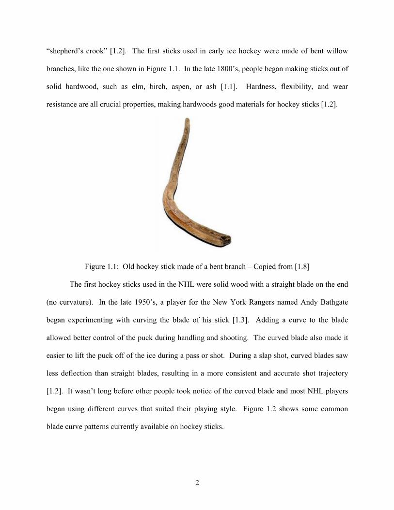
“shepherd’s crook” [1.2]. The first sticks used in early ice hockey were made of bent willow
branches, like the one shown in Figure 1.1. In the late 1800’s, people began making sticks out of
solid hardwood, such as elm, birch, aspen, or ash [1.1]. Hardness, flexibility, and wear
resistance are all crucial properties, making hardwoods good materials for hockey sticks [1.2].
Figure 1.1: Old hockey stick made of a bent branch – Copied from [1.8]
The first hockey sticks used in the NHL were solid wood with a straight blade on the end
(no curvature). In the late 1950’s, a player for the New York Rangers named Andy Bathgate
began experimenting with curving the blade of his stick [1.3]. Adding a curve to the blade
allowed better control of the puck during handling and shooting. The curved blade also made it
easier to lift the puck off of the ice during a pass or shot. During a slap shot, curved blades saw
less deflection than straight blades, resulting in a more consistent and accurate shot trajectory
[1.2]. It wasn’t long before other people took notice of the curved blade and most NHL players
began using different curves that suited their playing style. Figure 1.2 shows some common
blade curve patterns currently available on hockey sticks.
2

Figure 1.2: Common blade curve patterns – Copied from [1.9]
A player’s perceived feel of the puck on the stick is important in handling the puck down
the ice. Player’s prefer to feel small vibrations imparted in the stick while handling the puck so
that they don’t have to look directly at the puck to know its location on the blade. In addition, a
poor feeling stick can cause received passes to bounce off the blade, losing control of the puck.
Many players believe that wood sticks offer the best feel for the puck. Figure 1.3 shows some
modern wood sticks.
Figure 1.3: Wood hockey sticks with composite blade wraps – Copied from [1.10]
3

Players also began wrapping the blade of the stick with plastic materials to increase the
durability in the 1970’s to 1990’s [1.5]. This led to composite reinforced wood hockey sticks,
which are the only kind of wood sticks available today. Composite reinforced sticks provide a
good feel for the puck, but are among the heaviest sticks. In addition, wood has a tendency to
degrade or wear over time because wood is a natural material, and the stiffness of the stick can
vary by up to 40 % for sticks of the same model [1.2].
After the introduction of the curved blade and reinforced wood sticks, the hockey stick
market became stagnant for many years. The fairly recent outbreak of Dutch elm disease has
devastated the elm tree population, eliminating it as a commercially viable source of wood [1.2].
This sent manufacturers looking for new stick materials.
The first new material was aluminum. These sticks consist of a hollow aluminum shaft
with a wooden blade that is inserted in the bottom end of the shaft. Aluminum sticks are lighter
and more consistent than wood and also have good durability. Players found that aluminum
sticks have a cold, metallic feel and do not offer a good feel for the puck on the stick [1.2].
Aluminum shafts also tend to develop a permanent bend after repeated use. Some aluminum
hockey sticks with wood blade inserts are shown in Figure 1.4.
Figure 1.4: Aluminum hockey sticks with wood blade inserts – Copied from [1.10]
4

In the 1990’s, the price of composite materials, which were previously reserved mainly
for military applications, became more competitive, making them widely available to civilian
markets [1.6]. Hockey stick manufacturers have been among the list of sporting equipment
producers to take advantage of the benefits of composite materials.
The newest types of sticks, made entirely of composite materials, have revolutionized the
hockey stick market. These sticks are made of combinations of fiberglass, Kevlar, graphite,
resin, and/or carbon fiber [1.2]. A composite ice hockey stick is shown in Figure 1.5. There are
three different types of composite sticks: two-piece, one-piece, and true one-piece. Two-piece
sticks have a hollow composite shaft with a removable blade that is inserted into the bottom end
of the shaft, allowing players to use any blade pattern they prefer and the option to replace blades
if they break. One-piece sticks have the blade permanently bonded into the shaft at the junction,
or hosel. True one-piece composite sticks are the newest addition and are molded out of a single
piece of composite material, reducing overall weight and the stiffness in the hosel.
Figure 1.5: One-piece composite ice hockey stick – Copied from [1.9]
5
The first fully composite sticks were only marginally lighter than wood sticks and offered
players a very poor feel for the puck. In addition, they were very expensive and not very
durable. Further development of composite materials in sporting goods has led to a new kind of
composite stick that is manufactured to meet a number of player needs and offers many
advantages over wood sticks.
Composite sticks are the lightest on the market and degrade less than wood over time.
The stiffness, or flex, of the stick can be controlled during manufacturing to provide greater
consistency from one stick to another. In addition, the strength of composite materials enables
the production of more compliant sticks without sacrificing durability, which is preferable
among many players. Better control in the manufacturing of composite sticks has led to the
design of a shaft that is tapered toward the bottom. This is intended to reduce overall weight and
increase the amount of energy that can be transferred from the stick to the puck [1.2]. The cross-
sectional shape of the shaft can also be altered to accommodate player feel. One of the main
drawbacks to composite hockey sticks is their high cost, sometimes as much as $200 compared
to wood sticks that cost around $25.
Manufacturers and players claim that composite sticks perform better than wood sticks,
but little independent experimental research has been conducted to confirm or deny these claims.
This study sought to quantify hockey stick performance and vibration characteristics, and
experimentally compare the performance of several wood and composite hockey sticks.
Experimental methods were implemented to determine the effect of new technology on ice
hockey stick performance and vibration characteristics.
6
REFERENCES
[1.1] Davidson, John and Steinbreder, John, Hockey for Dummies, 2nd Edition, Wiley Publishing, Inc. New York (2000). ISBN: 0-7645-5228-7.
[1.2] Hache, Alain, The Physics of Ice Hockey, The Johns Hopkins University Press, Baltimore
and London (2002). ISBN: 0-8018-7071-2. [1.3] The Official Website of the National Hockey League: www.nhl.com
[1.4] Hoerner, E.F., The Dynamic Role Played by the Ice Hockey Stick, Safety in Ice Hockey, ASTM STP 1050 1, p. 154-163 (1989).
[1.5] Pearsall, D.J., Montgomery, D.L., Rothsching, N., and Turcotte, R.A. The Influence of
Stick Stiffness on the Performance of Ice Hockey Slap Shots. Sports Engineering 2, p.3-11 (1999).
[1.6] M. Buck and M. Dorf, Fiber-reinforced Plastics Improve Sporting Goods, Advanced
Materials & Processes 151 (6) (1997). [1.7] A. Villaseñor, A., Turcotte, R.A. and Pearsall, D.J. Recoil Effect of the Hockey Stick
During a Slap Shot. Journal of Applied Biomechanics, Vol. 22, p. 202-211 (2006). [1.8] Image copied from: placenamehere.com/objects/blog/oldblade.jpg [1.9] Images copied from: Epuck.com product descriptions, www.epuck.com [1.10] Images copied from: Falcon Sports Official Website, falconsports.com
7

CHAPTER TWO
BACKGROUND
2.1 Ice Hockey Pucks
Hockey pucks are made of a combination of approximately a dozen materials. Natural
rubber and a filler, usually carbon black or coal dust for the black color, make up about 90% of
the puck [2.1]. Additives such as sulfur and anti-oxidants make up the rest and help in the curing
process and contribute to the strength and hardness of the pucks [2.2]. Carbon also helps
improve wear resistance of the rubber in hockey pucks.
The ingredients are poured into a large, automatic mixer called a Banbury and then
extruded into soft rubber logs that are approximately three feet long [2.2]. These logs are sliced
into slugs that are roughly the size of pucks. Curing the slugs at 150 degrees C for about 22
minutes hardens the rubber [2.2]. The edges are knurled during the curing process and then
excess rubber left over from the mold is trimmed off, leaving a finished puck. Pucks used in the
NHL are made by a more expensive injection process in which the rubber is liquefied, injected
into a mold, and allowed to set, allowing the puck maker better control over the final product
[2.2].
Previous research has examined the behavior of hockey pucks at low speeds, but no
literature exists to characterize them at game speeds, which can reach 100 miles per hour in
professional play [2.1]. Drop tower tests, in which the puck is dropped from a known height and
the rebound height is measured have been performed on pucks to examine their elasticity. This
test is described in more detail in Section 2.1.1. Manufacturers test the rubber compound before
it is cured by placing a sample in a rheometer, which analyzes the curing curve and hardness of
8
the rubber. The curing curve is then compared to a pre-defined quality curve, which determines
if the batch passes inspection. In this study, pucks were characterized by their impact properties
at game speeds. The coefficient of restitution, or e, provided a measure of the puck’s elasticity,
while the dynamic stiffness, or kd, provided a measure of its dynamic hardness.
Pucks are often frozen before use in play in order to reduce their bounciness, allowing for
better control by the players. In addition, freezing pucks to the temperature of the ice before play
ensures uniform response throughout a game by keeping the puck temperature uniform. During
play, pucks are moved up and down the ice mainly by the sticks of the players. The speed of the
puck during play varies greatly depending on whether a player is passing, handling, or shooting
the puck. Previous studies have found that shot speeds can easily achieve 80 miles per hour in
elite play, with the fastest shooters in the 100 mile per hour range [2.1, 2.3, 2.4]. Several
different brands of pucks are available to players in the commercial market. Pucks in this study
were characterized for different brands, speeds, and temperatures.
2.1.1 Coefficient of Restitution
When two solid bodies undergo a collinear collision, reaction forces act in opposite
directions on the two bodies, changing the incident speed of the bodies. These reaction or
contact forces cause compression in the small area of the bodies that are in contact, or the contact
area [2.5]. During this compression, kinetic energy is transferred to stored elastic strain energy
in the bodies. At some point, the contact forces bring the approach speeds of the bodies to zero
and the stored elastic energy in the solids is returned to kinetic energy, forcing the bodies apart
until they separate with some resulting velocity [2.5]. This portion of the collision is termed
restitution. In the compression and restitution phase, some energy is always lost, typically due to
permanent deformation of the layers of atoms at the colliding surfaces [2.6].
9

The coefficient of restitution (e), is a measure of the elasticity of a collision. For two
colliding objects, it is defined as a ratio of the relative normal velocity of the objects after an
impact to their relative normal velocities before impact. More specifically,
⎟⎟⎠
⎞⎜⎜⎝
⎛−−
−=21
21
VVvve (2.1)
where v1 and v2 are the post-impact rebound speeds and V1 and V2 are the incident speeds of
objects 1 and 2, respectively. The negative sign in Equation 2.1 is due to the change in direction
of the velocities of the objects after a collision. In this case, the velocity can be considered
positive when the objects are moving toward each other and negative when they are moving
away from each other. Throughout the duration of this paper, a capital V denotes incident speed,
while a lowercase v denotes the post-impact speed.
The coefficient of restitution is a measure of the amount of kinetic energy that is lost in a
collision [2.7]. A perfectly elastic collision would have e = 1, while a perfectly inelastic
collision would have e = 0 [2.8]. A typical collision will have a coefficient of restitution value
lower than e = 1 due to energy losses from permanent deformation, internal modes of oscillation,
or a slow recovery to the original shape [2.9]. Some researchers attempt to predict e using
models that account for factors that include material stiffness, energy losses, or vibration [2.5].
Developing a coefficient of restitution model is out of the scope of this work, but Equation 2.1 is
still an accurate equation to measure e.
The idea of coefficient of restitution began with Isaac Newton examining collisions of
identical spheres. He recognized that only normal velocity components are important when
determining the resulting velocity of two objects after a collision [2.6]. Hodgkinson (1834)
examined collisions between dissimilar spheres and determined that the e is not a constant, but is
10

a function of the relative velocity of the colliding objects as well as the stiffness of the material
of each object [2.6].
In general, e for two colliding bodies depends on the elastic properties of both bodies, but
under some conditions may depend almost entirely on the elastic properties of only one body.
For example, if a very elastic ball, such as a tennis ball, is impacted on a very rigid wall, then the
resulting value of e provides a measure of the elasticity of the ball as long as there is no
significant deformation in the wall [2.8]. In this case, it would be appropriate to assume that the
coefficient of restitution is an inherent property of the ball, regardless of the rigid surface it is
impacted against [2.8]. If one of the objects in the collision is rigid and stationary, then Equation
(2.1) reduces to:
1
1
Vve −= (2.2)
Values for e are often used in sports as a measure of ball liveliness. For various sports balls e is
usually determined by shooting the ball at a rigid wall and measuring the inbound and rebound
speeds [2.10]. The coefficient of restitution has been investigated for a variety of sporting balls
and spherical objects, including golf balls, cricket balls, tennis balls, baseballs, and softballs.
If an object is dropped onto a surface that has a much larger mass than the object, then e
can be determined from the square root of the ratio of the rebound height to the drop height [2.8].
This procedure is referred to as a standard drop tower test, or drop test. The theory comes from
balancing the kinetic energy of a moving ball immediately before and after impact to the
potential energy of the ball in the air at both the drop height and final bounce height. That is, for
a ball with mass m that is dropped from a known height, h1 and rebounds to a measured height of
h2:
11

2
2
2
1
2
2121
emV
mv
mghmgh
i
r== (2.3)
where Vi and vr are the velocities at the instant before and after contact, respectively, and g is the
gravitational constant.
Vincent (1898-1900) and Raman (1918) expanded upon Hodgkinson’s work by
examining the repeatability of a collision of spheres over a range of approach speeds. They
found that as speed approaches infinity, e approaches zero (perfectly inelastic) and that as the
speed approaches zero, e approaches one (perfectly elastic) [2.6]. More recent studies have
shown that e decreases linearly with increasing incident speed for golf balls, baseballs, softballs,
and tennis balls over a finite speed interval ranging from 50 – 110 mph [2.11, 2.12, 2.13].
The decrease in e with increasing incident speed for a ball dropped on a rigid block can
be attributed to three major energy loss mechanisms [2.13]:
1. Increased excitation of internal waves or vibration modes in the block and/or the ball
2. Increased plastic deformation or the rigid wall or block
3. Viscoelastic behavior of the rigid block or ball.
Rayleigh (1906) estimated the fraction of energy stored in the fundamental vibration mode for
two slowly colliding spheres is about 0.02Vi/c, where c is the velocity of sound in the ball
material and Vi is the incident speed [2.7]. While this is quite small for many realistic scenarios,
it does identify the dependence of e on speed due to an increase in vibration with increasing
speed.
Limited testing has been done to determine e of hockey pucks at slow speeds. Standard
drop tests on a rigid surface have found the e of hockey pucks to range between 0.45 – 0.55 for
room temperature pucks and 0.12 – 0.27 for frozen pucks [2.1]. These tests were conducted at
12

low speeds, far from the speeds representative of game play. Gerl and Zippelius (1998) studied
the coefficient of restitution for elastic disks and found, like spheres, that it is a function of initial
relative velocity and the elastic properties of the disks [2.7]. Collisions were found to be elastic
for vanishing relative velocity (the quasistatic case) and increasingly inelastic for increasing
relative velocity [2.7].
As previously mentioned, pucks are often frozen prior to use in play in order to reduce
bouncing of the puck and increase the controllability for players. Freezing them prior to their
contact with the ice also prevents puck cooling during play, ensuring uniform response
throughout the duration of play. Previous slow speed puck testing shows that e decreases by
over half when pucks are frozen [2.1]. The e of softballs and baseballs has also been shown to
decrease with decreasing temperature [2.14, 2.15]. As the ball is heated, the material becomes
softer. A softer ball will deform more, retaining less kinetic energy and therefore having a lower
e than a hard ball [2.16].
ASTM Standard F1887-02 describes a method for determining the coefficient of
restitution of baseballs and softballs and is used in ball certification processes [2.17]. This
standard describes the coefficient of restitution as “a numerical value determined by the exit
speed of the ball after contact divided by the incoming speed of the ball before contact with a
massive, rigid, flat wall.” The e of hockey pucks was found in an analogous manner, and
therefore, all e values determined in this study are calculated using equation (2.2) unless
otherwise stated.
2.1.2 Dynamic Stiffness
Hockey pucks made by Viceroy are tested for their tensile strength and hardness in a
quasi-static manner [2.2]. These measurements to not account for the fact that the dynamic
13

properties of a puck may differ from its static properties [2.9]. Currently, no data exists in the
literature about the dynamic hardness of hockey pucks.
Previous studies have suggested that the performance of sports balls can be more
completely characterized by using a dynamic hardness method [2.9, 2.18, 2.26, 2.10]. One
important factor in making a good puck is achieving the right hardness [2.2]. If a puck is too
hard, it can cause excessive injury and break the glass surrounding the ice rink. If a puck is too
soft, it will wear quickly and deaden when it hits the boards. During a collision, localized
compression occurs in the contact area. This compressed area between the bodies acts like a
short, stiff spring that is compressed between the two bodies [2.5]. How stiff this “spring” is
depends on the hardness of the objects.
The hardness of an object can be viewed in terms of its peak impact force during a
collision with a rigid surface. A force measurement also provides useful information on the
behavior of the objects during the collision and the elastic properties of the colliding bodies
[2.9]. Force vs. time data for a puck can be measured by impacting it against a strike plate with
rigidly mounted load cells. This has been done for a variety of balls, including golf balls, tennis
balls, superballs, baseballs, and softballs [2.10, 2.12, 2.9, 2.16, 2.18, 2.19].
The method for calculating the dynamic stiffness of an object originates from an energy
balance between the kinetic energy of the moving puck and the spring energy stored in the
compressed region of the puck at its maximum displacement. During the collision between a
puck and a rigid strike plate, the reaction forces in the contact area do work on the system,
compressing the puck during impact until the inbound velocity of the puck is zero (compression
phase) [2.5]. The compressed region then recoils, forcing the puck away from the strike plate
with some rebound velocity (restitution phase).
14
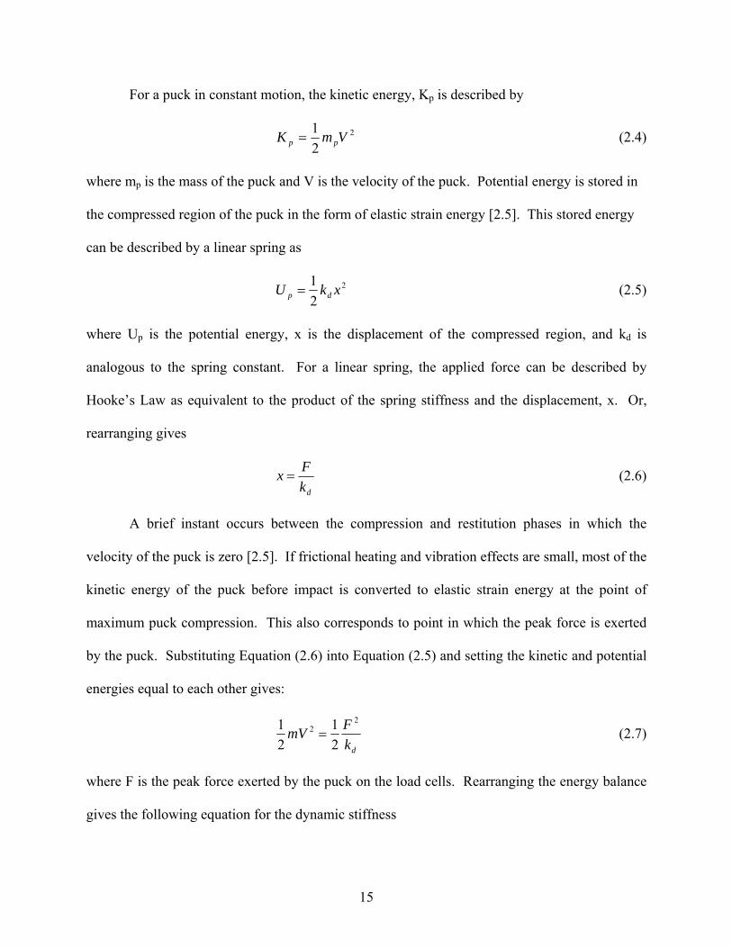
For a puck in constant motion, the kinetic energy, Kp is described by
2
21 VmK pp = (2.4)
where mp is the mass of the puck and V is the velocity of the puck. Potential energy is stored in
the compressed region of the puck in the form of elastic strain energy [2.5]. This stored energy
can be described by a linear spring as
2
21 xkU dp = (2.5)
where Up is the potential energy, x is the displacement of the compressed region, and kd is
analogous to the spring constant. For a linear spring, the applied force can be described by
Hooke’s Law as equivalent to the product of the spring stiffness and the displacement, x. Or,
rearranging gives
dkFx = (2.6)
A brief instant occurs between the compression and restitution phases in which the
velocity of the puck is zero [2.5]. If frictional heating and vibration effects are small, most of the
kinetic energy of the puck before impact is converted to elastic strain energy at the point of
maximum puck compression. This also corresponds to point in which the peak force is exerted
by the puck. Substituting Equation (2.6) into Equation (2.5) and setting the kinetic and potential
energies equal to each other gives:
dkFmV
22
21
21
= (2.7)
where F is the peak force exerted by the puck on the load cells. Rearranging the energy balance
gives the following equation for the dynamic stiffness
15
21
⎟⎟⎠
⎞⎜⎜⎝
⎛=
ipd V
Fm
k (2.8)
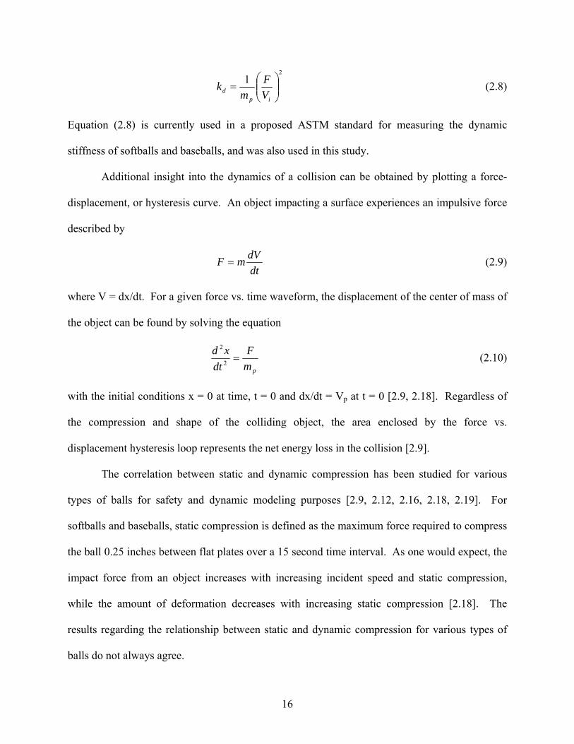
Equation (2.8) is currently used in a proposed ASTM standard for measuring the dynamic
stiffness of softballs and baseballs, and was also used in this study.
Additional insight into the dynamics of a collision can be obtained by plotting a force-
displacement, or hysteresis curve. An object impacting a surface experiences an impulsive force
described by
dtdVmF = (2.9)
where V = dx/dt. For a given force vs. time waveform, the displacement of the center of mass of
the object can be found by solving the equation
pmF
dtxd=2
2
(2.10)
with the initial conditions x = 0 at time, t = 0 and dx/dt = Vp at t = 0 [2.9, 2.18]. Regardless of
the compression and shape of the colliding object, the area enclosed by the force vs.
displacement hysteresis loop represents the net energy loss in the collision [2.9].
The correlation between static and dynamic compression has been studied for various
types of balls for safety and dynamic modeling purposes [2.9, 2.12, 2.16, 2.18, 2.19]. For
softballs and baseballs, static compression is defined as the maximum force required to compress
the ball 0.25 inches between flat plates over a 15 second time interval. As one would expect, the
impact force from an object increases with increasing incident speed and static compression,
while the amount of deformation decreases with increasing static compression [2.18]. The
results regarding the relationship between static and dynamic compression for various types of
balls do not always agree.
16

Hendee [2.12] found a linear correlation between static and dynamic compression for
baseballs at three different impact velocities. Later work by Chauvin [2.19] compared the static
compression of various baseballs and softballs to the dynamic compression obtained by firing
balls at a rigid wall with a pressure sensitive film. He found virtually no correlation between
static and dynamic compression values.
Cross [2.9] examined static and dynamic hysteresis curves for a tennis ball, a superball, a
golf ball, and a baseball. For all cases, he found that the area enclosed by the dynamic curve is
greater than the area enclosed by the static curve, indicating a greater energy loss under dynamic
conditions. The golf ball and the superball both showed fairly linear compression behavior
under static and dynamic conditions, while compression of the tennis ball and baseball was
nonlinear for both cases. All balls exhibited nonlinear behavior during restitution. Cross noted
that compression and restitution are nonlinear and frequency dependent, but a specific
relationship between static and dynamic behavior was not determined.
The effect of temperature on kd of sporting balls has not been studied in detail. Duris
[2.15] showed that as the temperature of softballs increased, kd decreased. As the temperature of
the material increases, it becomes softer. Following Chauvin’s logic [2.16], a softer (warmer)
ball will deform more easily than a hard (cold) ball, exerting a smaller force upon impact.
Thus far, compression and restitution behavior has been considered in terms of a material
that acts as a linear spring. The same treatment can also be considered in terms of a nonlinear
spring, which is described by the relationship
nn xkF = (2.11)
17
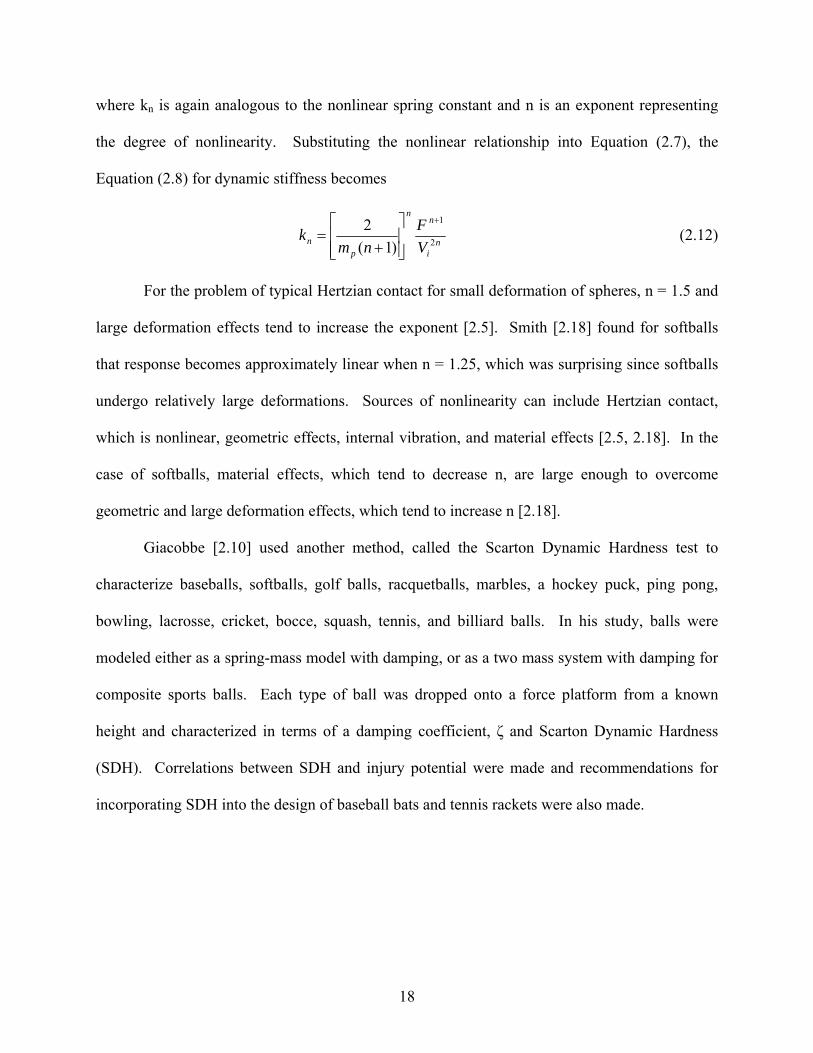
where kn is again analogous to the nonlinear spring constant and n is an exponent representing
the degree of nonlinearity. Substituting the nonlinear relationship into Equation (2.7), the
Equation (2.8) for dynamic stiffness becomes
ni
nn
pn V
Fnm
k 2
1
)1(2 +
⎥⎥⎦
⎤
⎢⎢⎣
⎡
+= (2.12)
For the problem of typical Hertzian contact for small deformation of spheres, n = 1.5 and
large deformation effects tend to increase the exponent [2.5]. Smith [2.18] found for softballs
that response becomes approximately linear when n = 1.25, which was surprising since softballs
undergo relatively large deformations. Sources of nonlinearity can include Hertzian contact,
which is nonlinear, geometric effects, internal vibration, and material effects [2.5, 2.18]. In the
case of softballs, material effects, which tend to decrease n, are large enough to overcome
geometric and large deformation effects, which tend to increase n [2.18].
Giacobbe [2.10] used another method, called the Scarton Dynamic Hardness test to
characterize baseballs, softballs, golf balls, racquetballs, marbles, a hockey puck, ping pong,
bowling, lacrosse, cricket, bocce, squash, tennis, and billiard balls. In his study, balls were
modeled either as a spring-mass model with damping, or as a two mass system with damping for
composite sports balls. Each type of ball was dropped onto a force platform from a known
height and characterized in terms of a damping coefficient, ζ and Scarton Dynamic Hardness
(SDH). Correlations between SDH and injury potential were made and recommendations for
incorporating SDH into the design of baseball bats and tennis rackets were also made.
18

2.2 Ice Hockey Sticks
2.2.1 General Trends in Ice Hockey Sticks
Hockey sticks are fabricated from wood, aluminum, or most recently composite
materials. The stick consists of the shaft, or the straight, long, handle portion, and the blade, or
the curved portion on the bottom of the stick used for moving the puck (Figure 2.1). Most
players wrap cloth tape around the top of the shaft for better grip and around the blade to cushion
the puck, making it easier to control.
Figure 2.1: Hockey stick components
The National Hockey League (NHL) regulates the dimensions of legal hockey sticks
[2.20]. These regulations mandate that sticks shall not exceed 63 inches in length from the heel
of the blade to the end of the shaft, and the blade shall not exceed 12.5 inches from the heel to
the toe. Blades must be between 2-3 inches in height and have beveled edges. In addition, the
NHL requires that “the curvature of the stick shall be restricted in such a manner that the
19

distance of a perpendicular line measured from a straight line drawn from any point at the heel to
the end of the blade to the point of maximum curvature shall not exceed three-quarters of an
inch,” as illustrated in Figure 2.3 [2.20]. While allowable dimensions are specified, there are no
regulations concerning the materials used in hockey stick construction.
Figure 2.2: Measurement of blade curvature – Copied from [2.20]
When selecting a stick, players are most concerned with durability, weight, the feel of the
puck on the stick, blade curve pattern, and stiffness of the shaft. There are many different blade
patterns available to suit a variety of player preferences. Blade patterns are chosen to suit
different styles of handling and shooting the puck. The general shape of the curve is classified as
either a heel, mid, or toe curve. This classification corresponds to where the majority of the
curve is located. Blades are then classified according to their curve depth as slight, moderate, or
deep. Finally, the face angle of the blade is rated as closed, slightly open, or very open [2.21].
Sticks are also rated by their stiffness (or flex), and their lie. The stiffness is typically
printed on the shaft of the stick and corresponds to the amount of force (usually in pounds)
required to deflect or bend the shaft one inch [2.1]. The span used to measure the stiffness of
hockey sticks is not defined in the literature. Adult sticks usually range from 75 – 115 stiffness
ratings. During shooting, the stick is deflected (loaded) and the energy stored in the stick is
transferred to the puck as it is released. Previous studies have measured the stiffness by
supporting the ends of the stick and deflecting the middle, as in a three point bend test [2.3,
2.22]. The concept of stick loading is discussed in greater detail in the next section. The amount
20
of loading a player can achieve during a shot is determined by both the player strength and the
stiffness of the stick.
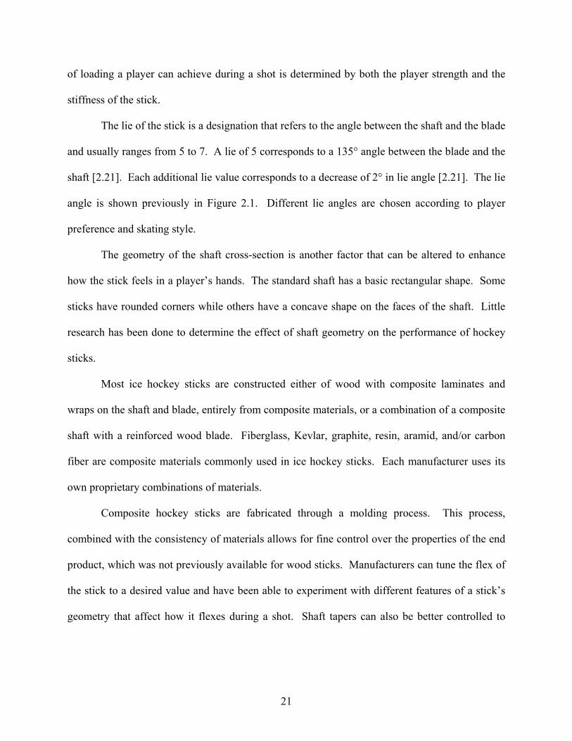
The lie of the stick is a designation that refers to the angle between the shaft and the blade
and usually ranges from 5 to 7. A lie of 5 corresponds to a 135° angle between the blade and the
shaft [2.21]. Each additional lie value corresponds to a decrease of 2° in lie angle [2.21]. The lie
angle is shown previously in Figure 2.1. Different lie angles are chosen according to player
preference and skating style.
The geometry of the shaft cross-section is another factor that can be altered to enhance
how the stick feels in a player’s hands. The standard shaft has a basic rectangular shape. Some
sticks have rounded corners while others have a concave shape on the faces of the shaft. Little
research has been done to determine the effect of shaft geometry on the performance of hockey
sticks.
Most ice hockey sticks are constructed either of wood with composite laminates and
wraps on the shaft and blade, entirely from composite materials, or a combination of a composite
shaft with a reinforced wood blade. Fiberglass, Kevlar, graphite, resin, aramid, and/or carbon
fiber are composite materials commonly used in ice hockey sticks. Each manufacturer uses its
own proprietary combinations of materials.
Composite hockey sticks are fabricated through a molding process. This process,
combined with the consistency of materials allows for fine control over the properties of the end
product, which was not previously available for wood sticks. Manufacturers can tune the flex of
the stick to a desired value and have been able to experiment with different features of a stick’s
geometry that affect how it flexes during a shot. Shaft tapers can also be better controlled to
21
lower the kick point. The kick point is the portion of the shaft that deflects the most during shaft
loading.
To date, the effects of these changes in stick characteristics on shot performance is not
fully understood [2.23]. It is generally agreed that factors such as physical attributes and skill
level of the player, mechanical properties of the stick, and the environment can all play a role in
determining shot performance. The effect of specific stick characteristics on shot speed is still
not well understood [2.23, 2.24, 2.4].
2.2.2 Stick and puck interactions
The hockey stick is used mainly to move the puck around on the ice. Stick handling
refers to the method of maneuvering the puck along the ice in front of a player. Stick handling is
also used to quickly move the puck around another player or stick. During stick handling,
players prefer to have a good feel for vibrations in the stick resulting from small puck impacts.
This allows them to know where the puck is relative to the stick without having to look down.
The stick is also used to pass the puck to another player and to shoot the puck at the net.
Four methods are used to shoot the puck: the wrist shot, the slap shot, the snap shot, and the
backhand shot. In any type of shot, the stick contacts the ice ahead of the puck and the shaft is
deflected, or loaded. The stick then comes in contact with the puck, and the shaft recoils,
propelling the puck in addition to the initial swing speed as it leaves the blade. The amount of
shaft loading that occurs is dependent on the player strength, stick stiffness, and the type of shot.
In a wrist shot, the puck is placed on the heel of the blade slightly behind the player. The
player makes a forward sweeping motion with the stick, pushing the puck along the ice and
eventually releasing it from the toe of the blade. The wrist shot is favored for its quick release
and highest accuracy of all types of shots.
22

The backhand shot is a variation of the wrist shot. In this case, the puck is placed toward
the heel on the backhand side of the blade. A sweeping motion is performed as the puck rolls
along the blade toward the toe. The puck is then released from the toe of the blade in a smooth,
sweeping motion. The backhand shot is advantageous when the player is not facing the goal and
provides fair shot accuracy with reduced power.
The snap shot is an abbreviated form of the slap shot. It employs a short backswing in
which the stick is raised off the ice and behind the puck. The player then swings the stick toward
the puck (downswing phase), contacting the ice shortly ahead of the puck and preloading the
shaft (preloading phase). The blade then contacts the puck and the shaft recoils before releasing
the puck. The snap shot has a faster release time and better accuracy than the slap shot.
The slap shot is the fastest method of moving the puck and can be completed either as a
stationary shot or while moving [2.25]. The slap shot involves six phases: backswing,
downswing, preloading, loading, release, and follow through [2.23, 2.25]. During the preloading
phase, the stick contacts the ice six to twelve inches in front of the puck, causing bending in the
shaft [2.23]. In this phase, kinetic energy is translated to elastic strain energy that is stored in the
shaft [2.25]. The deflected stick then contacts the puck during the loading phase, which lasts
approximately 30-40 ms [2.25]. During this contact time the stick recoils and elastic strain
energy from the recoiling shaft is transmitted to the puck in addition to the kinetic energy of the
swinging stick. The puck is subsequently released from the stick toward the target at the end of
the contact time or loading phase. The slap shot is the fastest, but also least accurate method of
shooting the puck.
Previous studies have found puck velocities up to 110 miles per hour during game play
[2.3]. Average puck velocities resulting from slap shots for elite and collegiate players have
23
been found in the range of 65-80 mph [2.23, 2.24, 2.25]. Most of the previous studies to
investigate slap shot characteristics have focused on technical aspects of skill execution with
little regard for stick characteristics [2.23]. The hockey stick performance metric developed in
section 2.3 was based on a model of a slap shot. The slap shot will now be discussed in greater
detail.
2.2.3 The Slap Shot
The slap shot is the fastest and most dramatic method of shooting the puck [2.25]. It is
employed 26% of the time by forwards and 54% of the time by defensive players in game play
[2.24]. Previous studies on the slap shot have investigated the biomechanics of shooting, the
effects of bending stiffness of the shaft [2.23], geometry of the shaft [2.22], and player skill level
[2.24, 2.25]. These studies found that the predominant factors in shot performance were player
skill level and the movement patterns of elite players compared to recreational players [2.25].
Little is understood about the effect of the stick’s physical features or the mechanical factors
regarding movement and contact time on the resulting velocity of the slap shot [2.22, 2.23, 2.25].
Several factors are generally believed to be important in shooting, including: velocity of the
lower end of the stick prior to contact with the ice, preloading of the stick, elastic stiffness
characteristics of the stick, and contact time with the puck [2.23, 2.25].
Early researchers in the 1960s and 1970s sought an understanding of the kinematics of a
slap shot and its injury potential in hockey shots [2.3]. Such studies were concerned with the
technical aspects of shooting regardless of the stick type [2.23]. In 1978 Sim and Chao [2.26]
used cinematographic analysis to conduct an in-depth biomechanical analysis of hockey shots.
The main goals were to measure the speeds of a skating player, the stick, and the puck during
shooting. Skater velocities were found in the range of 20-30 miles per hour and relative angular
24
velocity of the stick ranged from 20 - 30 radians per second. They found puck velocities up to
90 miles per hour for high school hockey players and up to 120 miles per hour for college and
professional players.
A more in-depth biomechanical analysis was performed by Marino in 1998 [2.4]. Key
results highlighted four mechanical factors as being important in the performance of shooting.
These factors were: (1) velocity of the lower end of the shaft prior to contact with the ice, (2)
preloading of the stick, (3) elastic stiffness characteristics of the stick, and (4) contact time with
the puck. Still, the direct relationship between mechanical properties of the stick and shot
velocity was not determined.
Hoerner [2.3] summarized the results of several investigations into wood stick durability
that were completed in the late 1970’s-late 1980’s. He found the following five failure modes
for hockey sticks during slap shots: junction of blade and shaft or hosel (44%), mid-shaft break
(16%) or delamination (15%), and blade break (14%) or delamination (11%). Examining broken
sticks, he determined some main variables are directly related to the durability and longevity of a
hockey stick. These variables included width of the handle, thickness of the handle, and the
mode of rigidity of the shaft to a plane parallel to the blade.
Also summarized by Hoerner [2.3] were several studies that determined the forces at
different points on the stick and the deflection of the shaft during wrist and slap shots.
Deflections in the shaft were 13° for a stiff stick and 15° for a flexible stick, which were twice
the deflections seen for wrist shots. The most important force in shooting was found to be at the
location of the lower hand. These studies also confirmed that the speed of shooting is directly
related to the acceleration impact of the stick in the forward, downward phase of the shot
25

movement. This demonstrated that a more flexible stick required a smaller force at the time of
impact than a more rigid one to obtain the same puck speed.
Few new developments in the research of hockey slap shots were made in the 1990’s.
The advent of new materials and greater selection in hockey stick properties inspired new
research into the effect of the characteristics of the stick itself on the performance of hockey
shots. Wider availability of high speed analysis techniques also contributed to the renewed
interest in hockey stick research [2.27].
Pearsall, et al. (1999) investigated the effect of stick stiffness on the performance of ice
hockey slap shots [2.23]. This study attempted to verify the belief by players and coaches that a
stiffer stick will permit greater force to be applied to the puck and thus yield a higher shot
velocity. Six elite male ice hockey players performed slap shots with composite hockey sticks of
four different stiffnesses that are commonly used by players. The stiffnesses used were rated at
13, 16, 17, and 19 KN/m. High speed video and force platforms were used to analyze the speed
and reaction forces in three dimensions for each shot.
Results showed significant differences in maximum puck velocity for shaft stiffness,
subject, and the interaction of subject and stiffness. The only statistically significant differences
according to shaft stiffness were in the most flexible and the second stiffest sticks. The most
flexible stick had the highest puck velocity and the lowest vertical peak reaction force. The
second stiffest stick had the lowest puck velocity and the highest vertical peak reaction force;
however, the greater reaction force did not translate to greater shot velocities. In addition, peak
shaft deflection showed an inverse relationship with shaft stiffness, with peak deflections in
order from most flexible to stiffest of 20.4°, 18.7°, 18.4°, and 17.9°. The interaction between
subjects and stiffness was found to account for 67% of the variation in peak shaft deflection. In
26

general, the stiffness of the stick used in a slap shot seemed unimportant in determining the
kinematic behavior of the stick. Subjects appeared to be more important in determining the
velocity of the shot than the stick characteristics.
Further research by Moreno, Wood, and Thompson (2004) studied the effects of
technique and stick dynamics in the performance of standing snap shots [2.22]. One elite ice
hockey player performed snap shots with two different sticks. The first was a standard
composite stick with a rectangular cross-section (stick 1) and the second was a composite stick
with wood veneer siding and a double concave shaft shape (stick 2). A quasi-static
characterization of force vs. deflection was found by a three point bend test for both sticks. An
essentially identical linear relationship was found for each stick.
During shooting trials the two sticks exhibited different loading diagrams. In all trials,
stick 2 reached a higher peak force in a shorter amount of time than stick 1, but recorded puck
velocities were very similar for both sticks (stick 1 – 23.6 +/- 0.6 m/s and stick 2 – 23.3 +/- 0.6
m/s). The angular velocity of the hosel after the blade leaves the ice was found to be drastically
higher for stick 2 (896 deg/s) than for stick 1 (281 deg/s), indicating that stick 2 recovers from
being deflected much faster than stick 1. They concluded that changing the shape of the shaft
from standard rectangular to a double concave design increases the recovery rate and maximum
deflection, yet the overall velocity of the puck stays the same. No comment was made regarding
the effect of the added wood veneers to the double concave stick design. It was postulated that
the faster recovery time of stick 2 allowed the puck to reach its end velocity faster than for stick
1, giving the player a quicker release and the goalie less time to react to the shot.
More recent studies have focused on the mechanical parameters of shooting, such as the
recoil effect (unloading of the deflected shaft) of the hockey stick [2.25] and the effect of player
27

skill on blade contact and deformation in three dimensions during slap shots [2.24]. Villaseñor
found that both recreational and elite players applied the same magnitude of force to the puck
during slap shots, but the elite group produced greater stick recoil. Elite players had a longer
blade-puck contact time during the recoil phase of the shot, resulting in greater puck velocities
than recreational players [2.25]. Findings suggested that elite players were also able to generate
a lower kick point during shaft loading and unloading, therefore utilizing the recoil effect with
greater efficiency than recreational players [2.24, 2.25].
Lomond et al. (2007) recognized that little was known about the timing parameters
between the stick and puck within the ice hockey slap shot even though proper timing and
movements have been identified as an essential component in successful striking tasks [2.24].
They sought to quantify the influence of player skill on stationary slap shot performance during
the critical period of blade-ground contact.
A unique recoil phase was identified within the duration of the slap shot for both elite and
recreational players, during which the deflected shaft of the stick straightened, transferring
energy to the puck. This phase was longer for elite players and at times relatively nonexistent for
recreational players. Greater puck velocity was found in the elite players due to timing
adjustments that increased linear displacement, velocity, and acceleration of the stick and puck
during the rocker phase compared to recreational players who utilized greater rotational
variables. Contrary to popular industry opinion, the different construction parameters of blades
currently on the market did not affect the blade’s global position or orientation during the slap
shot, suggesting that greater shot performance came from player movements and/or parameters
of the stick.
28

In previous research regarding the execution and performance of ice hockey slap shots,
subjects performed shots that were then analyzed in a lab setting. Performance has either been a
function of player skill or subject variability has shown significant interference in the
performance results. The current study developed a stick performance measure that is
independent of player movements or skill level. Such a performance measure would allow direct
comparison between sticks and stick characteristics, regardless of player interference or skill
level.
2.3 Hockey Stick Performance Metrics
It is desirable to have a standard measure of performance, regardless of the player using the
stick, as an objective measure that can be used to compare the efficacy of one stick to another.
This measure should relate the performance of a stick at game speeds, regardless of player skill
level or strength.
The concept of a high speed performance measure that describes a collision in the field of
play began with the bat-ball sports of softball and baseball. Various measures such as Bat
Performance Factor (BPF), Bat-Ball Coefficient of Restitution (BBCOR), Ball Exit Speed Ratio
(BESR), and Batted-Ball Speed (BBS) are used to describe the efficiency of a high speed bat-ball
collision. These bat performance metrics have been used by regulatory agencies such as the
National Collegiate Athletic Association (NCAA), the Amateur Softball Association (ASA), and
United States Specialty Sports Association (USSSA) to regulate the performance of bats allowed
on the field of play.
ASTM F 2219-04 [2.28] describes a standard method for measuring and calculating these
quantities. The basis for these performance metrics is a momentum balance between a ball and a
29
bat. A ball is fired from a high speed cannon at a stationary pivoted bat with a known velocity.
The rebound speed of the ball after hitting the bat is measured and performance measures are
calculated. Analogous tests have been performed for cricket, tennis, and golf [2.29, 2.30]. The
same reasoning was applied here to a collision between a stick and a puck.
During a stick-puck collision momentum is conserved. A stick-puck collision
momentum balance is of the form
2211 ωω IQvmIQVm pp +=+ (2.13)
where V1 and ω1 are the puck linear velocity (in/sec) and the stick angular velocity (rad/sec),
respectively, before impact, v2 and ω2 are the puck linear velocity and the stick angular velocity
after impact, mp is the mass of the puck (oz), Q is the impact location measured from the pivot
point (in), and I is the stick moment of inertia, or MOI (oz-in2) measured about the same pivot
location. Figure 2.3 illustrates the sign convention used for determining the momentum of the
stick and puck.
For softball and baseball bats, ASTM F 2398-04 [2.31] describes a method for
determining the moment of inertia. In this standard the bat is modeled as a physical pendulum,
and the MOI is determined by measuring its period of oscillation, mass, and distance between the
pivot point and center of mass. A similar method was used for determining the MOI of hockey
sticks in this study. The axis of rotation was taken as perpendicular to the length of the shaft and
in a plane parallel to the blade. This can be pictured as coming out of the page in Figure 2.3.
30

( + ) ( - )
Figure 2.3: Sign convention definition
The inertia of a physical pendulum can be found from the equation
2
2
4πη agW
I t= (2.14)
where η is the period of oscillation of the stick (Hz), g is gravitational acceleration (in/sec2), Wt
is the total weight of the stick, and a is the distance (in) between the center of mass and the pivot
point. The period, η is an average value found by measuring the time for the stick to oscillate
through fifteen cycles.
The center of mass, or balance point (BP) can be found by measuring the mass at
distances of six inches and 42 inches from the handle end of the shaft. The BP is then calculated
as a weighted average, or
tWWW
BP 426 426 += (2.15)
where W6 and W42 are the weights of the stick at six inches and 42 inches from the end of the
stick. A schematic of the fixture used to measure the weight at six and 42 inches is shown in
Figure 2.4.
31

Figure 2.4: Schematic of the balance point fixture
The distance a between the pivot point and the balance point is then
lBPa −= (2.16)
where l is the distance measured from the end of the stick handle to the pivot point. The pivot
point was taken as 35 inches along the shaft from the handle end of the stick.
A stick with a higher MOI will have more momentum, and therefore more kinetic energy
available to transfer when it hits the puck. On the contrary, more energy is required from the
player to swing a stick of higher MOI at the same speed as one of lower MOI. The speed at
which a player can swing a bat, racket, or club depends on the MOI rather than the mass of the
striking implement [2.32]. The MOI itself is dependent on the mass, length, and mass
distribution of the stick. Two sticks can have the same mass and length, but different MOI if the
weight is distributed differently in one compared to the other.
Previous studies on the effects of MOI on swing speed of a striking implement have
found an inverse relationship between swing speed and MOI [2.32, 2.33, 2.34, 2.35]. These
studies examined baseball and softball bats, golf clubs, and simple rods. The effects on swing
speed due to MOI have been expressed in terms of a ball speed coming off the implement for
softball and baseball bats [2.33, 2.34] and tennis rackets [2.32]. In both cases curves of ball
speed vs. MOI were exponential in form, and Bahill [2.34] claimed that an optimum MOI value
exists for a given player to achieve the maximum ball speed. This optimum value is a trade-off
32
between how fast a player can swing an implement and the amount of momentum generated
from the inertia of the implement.
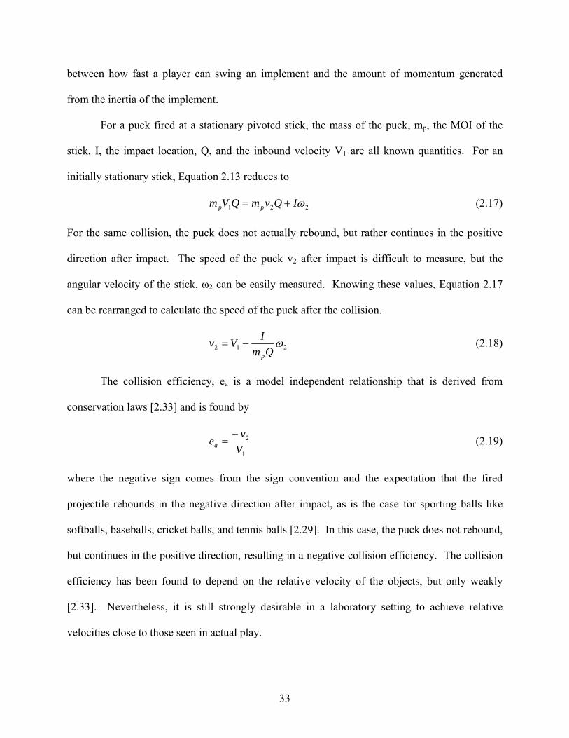
For a puck fired at a stationary pivoted stick, the mass of the puck, mp, the MOI of the
stick, I, the impact location, Q, and the inbound velocity V1 are all known quantities. For an
initially stationary stick, Equation 2.13 reduces to
221 ωIQvmQVm pp += (2.17)
For the same collision, the puck does not actually rebound, but rather continues in the positive
direction after impact. The speed of the puck v2 after impact is difficult to measure, but the
angular velocity of the stick, ω2 can be easily measured. Knowing these values, Equation 2.17
can be rearranged to calculate the speed of the puck after the collision.
212 ωQm
IVvp
−= (2.18)
The collision efficiency, ea is a model independent relationship that is derived from
conservation laws [2.33] and is found by
1
2
Vv
ea−
= (2.19)
where the negative sign comes from the sign convention and the expectation that the fired
projectile rebounds in the negative direction after impact, as is the case for sporting balls like
softballs, baseballs, cricket balls, and tennis balls [2.29]. In this case, the puck does not rebound,
but continues in the positive direction, resulting in a negative collision efficiency. The collision
efficiency has been found to depend on the relative velocity of the objects, but only weakly
[2.33]. Nevertheless, it is still strongly desirable in a laboratory setting to achieve relative
velocities close to those seen in actual play.
33
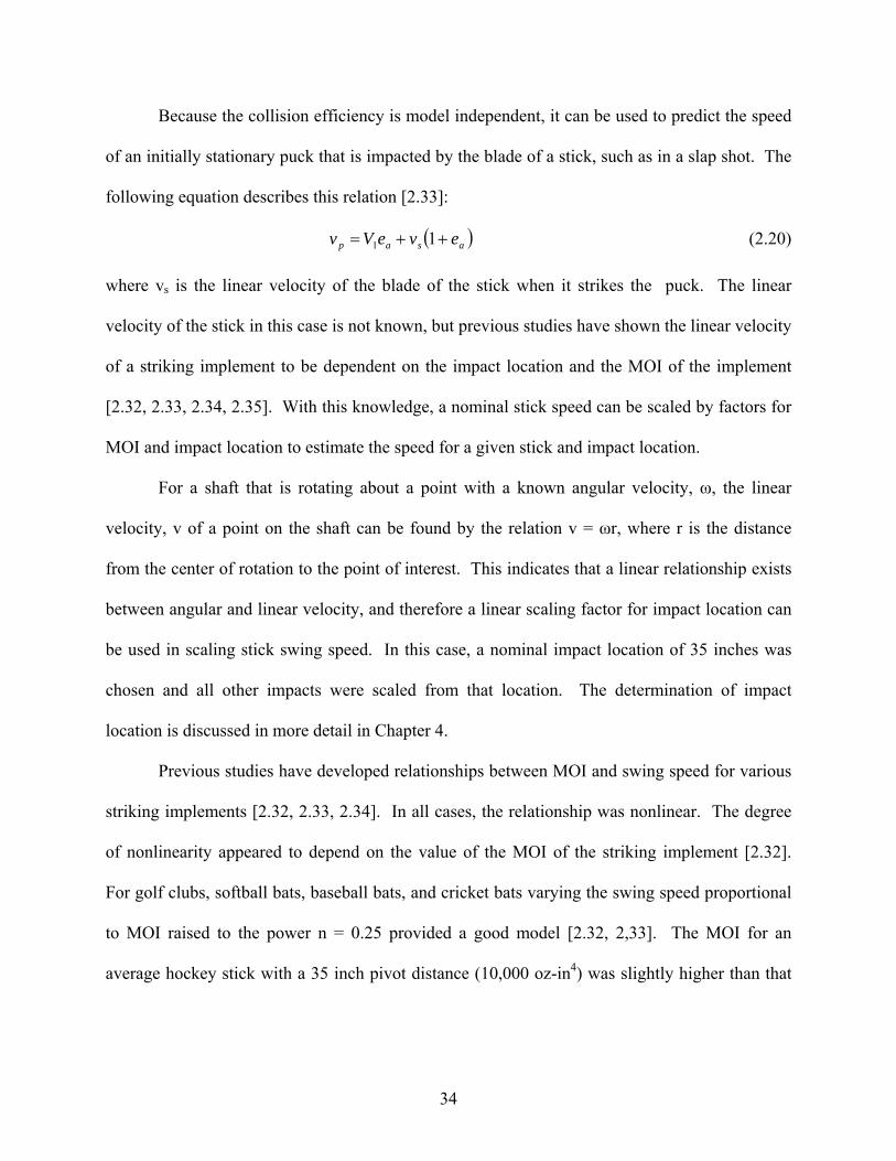
Because the collision efficiency is model independent, it can be used to predict the speed
of an initially stationary puck that is impacted by the blade of a stick, such as in a slap shot. The
following equation describes this relation [2.33]:
( )asap eveVv ++= 11 (2.20)
where vs is the linear velocity of the blade of the stick when it strikes the puck. The linear
velocity of the stick in this case is not known, but previous studies have shown the linear velocity
of a striking implement to be dependent on the impact location and the MOI of the implement
[2.32, 2.33, 2.34, 2.35]. With this knowledge, a nominal stick speed can be scaled by factors for
MOI and impact location to estimate the speed for a given stick and impact location.
For a shaft that is rotating about a point with a known angular velocity, ω, the linear
velocity, v of a point on the shaft can be found by the relation v = ωr, where r is the distance
from the center of rotation to the point of interest. This indicates that a linear relationship exists
between angular and linear velocity, and therefore a linear scaling factor for impact location can
be used in scaling stick swing speed. In this case, a nominal impact location of 35 inches was
chosen and all other impacts were scaled from that location. The determination of impact
location is discussed in more detail in Chapter 4.
Previous studies have developed relationships between MOI and swing speed for various
striking implements [2.32, 2.33, 2.34]. In all cases, the relationship was nonlinear. The degree
of nonlinearity appeared to depend on the value of the MOI of the striking implement [2.32].
For golf clubs, softball bats, baseball bats, and cricket bats varying the swing speed proportional
to MOI raised to the power n = 0.25 provided a good model [2.32, 2,33]. The MOI for an
average hockey stick with a 35 inch pivot distance (10,000 oz-in4) was slightly higher than that
34
of a typical slow pitch softball bat (9000 oz-in4), but still within the range that is successfully
estimated when n = 0.25.
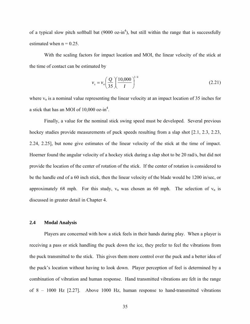
With the scaling factors for impact location and MOI, the linear velocity of the stick at
the time of contact can be estimated by
4/1000,1035
⎟⎠⎞
⎜⎝⎛⎟⎠⎞
⎜⎝⎛=
IQvv ns (2.21)
where vn is a nominal value representing the linear velocity at an impact location of 35 inches for
a stick that has an MOI of 10,000 oz-in4.
Finally, a value for the nominal stick swing speed must be developed. Several previous
hockey studies provide measurements of puck speeds resulting from a slap shot [2.1, 2.3, 2.23,
2.24, 2.25], but none give estimates of the linear velocity of the stick at the time of impact.
Hoerner found the angular velocity of a hockey stick during a slap shot to be 20 rad/s, but did not
provide the location of the center of rotation of the stick. If the center of rotation is considered to
be the handle end of a 60 inch stick, then the linear velocity of the blade would be 1200 in/sec, or
approximately 68 mph. For this study, vn was chosen as 60 mph. The selection of vn is
discussed in greater detail in Chapter 4.
2.4 Modal Analysis
Players are concerned with how a stick feels in their hands during play. When a player is
receiving a pass or stick handling the puck down the ice, they prefer to feel the vibrations from
the puck transmitted to the stick. This gives them more control over the puck and a better idea of
the puck’s location without having to look down. Player perception of feel is determined by a
combination of vibration and human response. Hand transmitted vibrations are felt in the range
of 8 – 1000 Hz [2.27]. Above 1000 Hz, human response to hand-transmitted vibrations
35

diminishes. Sports equipment manufacturers are concerned with optimizing the feel of their
equipment compared to their competitor’s.
Vibration patterns of an object or structure appear to be an unpredictable phenomenon,
but they are in fact very measurable. When a structural object is excited, it vibrates at specific
frequencies, called natural or resonant frequencies, and with specific deformation patterns. At a
resonant frequency, the response is maximized when compared to the stimulus [2.27]. Resonant
vibration is caused by an interaction between the inertial and elastic properties of the materials in
the structure [2.36].
The deformed shape of a vibrating object is termed its mode shape. Each resonant
frequency has exactly one mode shape for a given structural object. Under normal operating
conditions, a structure typically vibrates in complex combinations of several or all of its mode
shapes. Damping is a term that describes how quickly vibrations will decay in an object. Modal
analysis is a method of dynamically characterizing an object in terms of its frequency, damping,
and mode shapes.
Modal parameters are extracted by mechanically exciting a structure and measuring its
operating deflection shapes. Two types of modal testing are commonly used in practice: shaker
testing and impact hammer testing. In shaker testing an exciter, or shaker is fixed to the object of
interest and provides either a random or sinusoidal excitation to the object. The vibrational
response of the object is then observed at one or more locations. In impact hammer testing, an
impact hammer is used to excite the object with a measured input impulse at as many locations
as desired to define the mode shapes of the structure. The response is measured by a fixed
accelerometer on the object for each input excitation. A modal test in which the accelerometer is
36

fixed and the hammer impacts different locations is known as a roving hammer test [2.36].
Roving impact hammer tests were used in this work and will be considered in more detail.
A force transducer in the tip of the impact hammer can be used to measure the magnitude
of the impulse as a function of time. The responding motion of a fixed accelerometer can be
used to measure the response at a point as a function of time. By varying the frequency of the
input loading cycle, the amplitude of the response varies as the frequency of the input loading
changes [2.37]. This is seen by plotting the response in the time domain. Viewing the response
in the time domain can provide useful information about the damping of the system.
Mode shapes and resonant frequencies can be obtained by viewing the input and response
functions in the frequency domain. This data can be transformed from the time domain to the
frequency domain using the Fast Fourier Transform (FFT). The Frequency Response Function
(FRF) describes the input-output relationship between two points on a structure as a function of
frequency. It is defined as [2.36]:
)()(
InputFFTOutputFFTFRF = (2.22)
The FRF is a complex function with both real and imaginary parts that relates the output per unit
of input for each frequency. Peaks occur in the FRF at resonant or natural frequencies where the
time response was observed to have maximum response corresponding to the rate of oscillation
of the input excitation [2.37]. The amplitude of the peak describes the mode shape, while the
steepness of the peak describes the damping of that mode.
The simplest modal model is a single-degree-of-freedom (SDOF) system, which
corresponds to a single input (impact hammer) with a single output (accelerometer). This model
consists of three elements: a spring, a mass, and a damper. Energy enters the system through the
37

input excitation, causing oscillation, and is diminished through damping. The equation of
motion for a SDOF system is [2.38]:
)(tfkxxcxm =++ &&& (2.23)
where m is the mass, c is the damping coefficient, k is the spring stiffness, and f(t) is the sum of
the applied forces as a function of time. The displacement of the system is x and each dot
represents a time derivative of displacement. The equation (2.23) shows that vibration consists
of a balance between inertia, damping, spring, and excitation forces [2.39].
A SDOF system will have a single peak in the FRF, located at the natural frequency at
which it resonates. A more complex system will have many natural frequencies, each
corresponding to a different vibration mode. The response will appear more complex than that
of a SDOF system, but this system can be simplified by viewing it in terms of combinations of
SDOF systems [2.38]. The FRF for a SDOF system is defined as a function of frequency, ω by
the relation
⎟⎟⎠
⎞⎜⎜⎝
⎛+⎟⎟
⎠
⎞⎜⎜⎝
⎛−
=
nn
ik
H
ωωξ
ωω
ω
21
11)( 2 (2.24)
where ωn is the natural frequency and ξ is the critical damping factor [2.40]. Solving this
equation for the critical damping factor yields the damping rate, σn of the system:
2
22
1 ξξωσ
−= n
n (2.25)
Let us now consider a modal test for a hockey stick. Figure 2.5 illustrates the test setup
to characterize the bending modes of a hockey stick. In this case, bending is examined in the
plane of the stick that exhibits the most bending when the shaft is loaded during a shot. In order
to obtain mode shapes via a roving hammer test, the FRF must be obtained for several locations
38

along the length of the stick. This is done by impacting the stick at one inch intervals along its
length and measuring the response with an accelerometer that is fixed to a single location, in this
case the middle of the shaft.
Figure 2.5: Experimental setup for modal analysis of a hockey stick
As earlier mentioned, the FRF is a complex quantity with both real and imaginary parts,
or magnitude and phase. One method of analyzing FRF data is to plot the imaginary part of the
function. Quadrature picking describes a method in which the imaginary part of the FRF is
analyzed to find peaks. Each resonant frequency appears as a peak in the imaginary part of the
FRF. The phase of the signal is indicated by either a positive or negative peak [2.36].
Quadrature picking is a simple method to determine mode shapes of an object.
The imaginary portion of each FRF can be plotted as a function of location along the
length of the stick to show the deformation patterns, or mode shapes, for each resonant
frequency. Plotting the FRFs along the length of the stick produces a waterfall plot. A sample
waterfall plot showing the first four modes is below in Figure 2.6.
39

Figure 2.6: Sample waterfall plot for a hockey stick
Each mode is given a number, n, that corresponds to the number of peaks seen in the
mode shape. The mode number increases with increasing frequency. For each n-mode, n+1
nodes, or locations of zero movement during vibration will exist within the structure. These
node points remain stationary during oscillation and are important in determining the dynamic
behavior of a structure [2.39].
The range of frequencies that are excited in a modal test is determined by the type of tip
on the impact hammer that is used. A harder tip will excite a higher range of frequencies than a
softer tip [2.37]. This occurs because the contact time is shorter for a hard tip than for a soft tip.
In this work, a medium hardness tip was used because the frequencies of interest in testing
hockey sticks were found to be relatively low (below 1000 Hz).
40

The boundary conditions that are imposed during a modal test can have a significant
effect on the dynamic behavior of a system, and therefore must be carefully considered [2.40].
Typically boundary conditions that approximate service conditions are desired in vibration
testing. A free-free setup was used in this case by supporting the hockey stick on elastic supports
that allow the stick to vibrate freely when excited.
In an impact modal test, the desired location is impacted several times and the data is
averaged over the number of impacts. The coherence is a parameter that indicates how
accurately the dynamic characteristics of a structure are being characterized. The coherence
provides a measure of how much of the response is due to the input excitation vs. external noise
and/or nonlinearities in the system [2.40]. It is defined from the FRF data as:
yx
xyCσσ
σ= (2.26)
where σxy is the cross-correlation coefficient, σx is the input signal’s variance, and σy is the
output signal’s variance [2.39]. Derivation of the cross-correlation coefficient and signal
variance is outside the scope of this paper, and the reader is referred to [2.39, 2.40] for further
information. Coherence values are a function of frequency and range between zero and one. For
a coherence value of one, the tester can say with confidence that the input and output response
are directly linked. A coherence of zero indicates that they are not linked and the response is due
to external noise [2.40]. FRFs are unique for each combination of impact and accelerometer
location, so coherence cannot be used to compare data for multiple impact locations [2.40].
In a simple, hollow, one-dimensional system vibration modes can be categorized as either
flexural bending, or hoop modes. Flexural modes describe bending of the stick, while hoop
modes describe oscillation in the radial direction along the length of the stick. The hoop
frequencies are dependent on the wall thickness of the stick. Because a hockey stick is long and
41

slender, hoop modes occur at much higher frequencies than bending modes and were not
considered in this study. Figure 2.7 illustrates various bending modes for a hockey stick.
Figure 2.7: Flexural bending modes 1, 2, and 4 for a hockey stick (courtesy of Dr. Dan
Russell, Kettering University)
2.5 Summary
This chapter provided the background information necessary to introduce the
fundamental principles that were utilized for research in this study. In the first section, the
42
characteristics and manufacturing processes of ice hockey pucks were discussed. The mechanics
of a collision were also discussed in some detail. The concept of coefficient of restitution has
been introduced as a means of characterizing the elasticity of a puck. Little data exists regarding
e of hockey pucks, aside from slow speed e values for both room temperature and frozen pucks.
Coefficient of restitution has been shown to decrease with increasing speed for a variety of
sporting balls. It has also been shown to decrease with increasing temperature.
Another impact property, dynamic stiffness, was also introduced in this section. The kd is
a measure of the hardness of an object. It can be calculated by assuming the object behaves as a
linear spring and equating the kinetic energy before impact to the potential energy stored in
elastic deformation at the time of greatest deflection (peak impact force). Additional information
about the dynamics of a collision can be obtained from the force-deflection, or hysteresis curve,
which is found from force-time data during an impact.
Previous studies have shown hysteresis curves for different types of balls. Several
comparisons have been made between static and dynamic behavior, but the results are
conflicting. It has been shown that as speed increases, the peak force and the amount of energy
lost in the collision also increase. The peak force, and therefore kd, has also been shown to
decrease with increasing temperature for softballs and baseballs.
The next section of this chapter discussed ice hockey sticks and stick – puck interactions.
The impact of new technologies on the manufacturing and end characteristics of hockey sticks
was discussed. The slap shot was presented in detail, and the results of previous research
regarding the performance of hockey sticks and shots was discussed. Previous studies have all
employed test subjects performing various hockey shots. No previous studies have examined the
performance of ice hockey sticks regardless of the player using them.
43
The inertia of a swinging implement and its effects on swing speed were introduced. A
concept of a high speed performance measure that describes a collision was also presented.
Momentum concepts were used to examine the collision of a stationary stick and a moving puck
and develop a performance measure that described a moving stick and a stationary puck. Similar
test methods have been used to describe collisions for softball, baseball, and cricket.
Finally, the concepts of vibration and modal analysis were presented. The vibration
behavior of an object can be described in terms of its natural frequencies, mode shapes, and
damping. Modal analysis is a dynamic analysis tool that is used to determine these vibration
characteristics. It employs an impact hammer and a force transducer that measures the excitation
input and an accelerometer to measure the output response of the object. The input excitation
and output can be viewed in the frequency domain to determine the modal characteristics of an
object.
The concepts discussed in this chapter will be applied in subsequent chapters involving
the characterization of ice hockey sticks and pucks. The impact properties of hockey pucks will
be discussed in Chapter 3. The principles relating to stick characterization and performance
testing will be discussed in Chapter 4.
44
REFERENCES
[2.1] Hache, Alain, The Physics of Ice Hockey, The Johns Hopkins University Press, Baltimore and London (2002). ISBN: 0-8018-7071-2.
[2.2] Falconer, T. How Hockey Works, Equinox. January/February 1994. [2.3] Hoerner, E.F., The Dynamic Role Played by the Ice Hockey Stick, Safety in Ice Hockey,
ASTM STP 1050 1, p. 154-163 (1989). [2.4] G.W. Marino, Biomechanical Investigations of Performance Characteristics of Different
Types of Ice Hockey Sticks. Proceedings 1 of the International Society of Biomechanics of Sport, Konstanz, Germany p. 184-187 (1998).
[2.5] Stronge, William James, Impact Mechanics. Cambridge University Press, Cambridge,
United Kingdom (2000). ISBN 0-521-63286-2. [2.6] Barnes, G. The Study of Collisions. Am. J. Phys. 26 p. 5-12. (1957). [2.7] Gerl, F. and Zippelius, A., Coefficient of restitution for elastic disks, Physical Review E.
Statistical Physics, Plasmas, Fluids, and Related Interdisciplinary Topics 59 (2-B), p. 2361. (1999)
[2.8] Cross, R. The coefficient of restitution for collisions of happy balls, unhappy balls, and
tennis balls. Am. J. Phys. 68(11) p. 1025-1031. 2000. [2.9] Cross, R. The bounce of a ball, Am. J. Phys. 67(3), p. 222-227 (1999). [2.10] Giacobbe, P.A., Scarton, H.A., and Yau-Shing Lee, Dynamic Hardness (SDH) of
Baseballs and Softballs, ASTM STP 1313, p. 47-66, 1997 [2.11] Cochran, A.J. Development and use of one dimensional models of a golf ball. J. Sports
Sciences. Taylor and Francis, Ltd. London, UK (2002). [2.12] Hendee, S.P., Greenwald, R.M., Crisco, J.J. Static and Dynamic Properties of Various
Baseballs. J. App. Biomech. 14, p. 390-400 (1998). [2.13] Stensgaard, I., Laegsgaard, E. Listening to the coefficient of restitution – revisited. Am.
J. Phys. 69 (3), p. 301-305 (2001). [2.14] Drane, P.J. and Sherwood, J.A., Characterization of the effect of temperature on baseball
COR performance, Proceedings from the Eng. of Sport 5 (2), p. 59-65. 2004. [2.15] Duris, J.G., Experimental and numerical characterization of softballs, Master’s Thesis,
Washington State University, 2004.
45
[2.16] Chauvin, D.J., Carlson, L.E., A comparative test method for dynamic response of baseballs and softballs. International Symposium on Safety in Baseball/Softball, ASTM STP 1313, p. 38-46, 1997.
[2.17] ASTM F1887 Standard Test Method for Measuring the Coefficient of Restitution (COR)
of Baseballs and Softballs, ASTM International 2004. [2.18] Smith, L.V., Duris, J.G., and Nathan, A.M., Describing the Dynamic Response of
Softballs, Society of Experimental Mechanics, submitted August 2007. [2.19] Axtell, J.T., Experimental Determination of Baseball Bat Durability. Master’s Thesis,
Washington State University, 2001. [2.20] National Hockey League Official Rules 2006 – 2007. Triumph Books, Chicago, IL.
ISBN: 1-894801-03-2. [2.21] Davidson, John and Steinbreder, John, Hockey for Dummies, 2nd Edition, Wiley
Publishing, Inc. New York (2000). ISBN: 0-7645-5228-7. [2.22] D.A. Moreno, J.T. Wood, and B.E. Thompson, Dynamic analysis techniques for the
design of the ice hockey stick. The Engineering of Sport 5 (1) (2004). [2.23] Pearsall, D.J., Montgomery, D.L., Rothsching, N., and Turcotte, R.A. The Influence of
Stick Stiffness on the Performance of Ice Hockey Slap Shots. Sports Engineering 2, p.3-11 (1999).
[2.24] V. Lomond, R.A. Turcotte, and D.J. Pearsall, Three-dimensional analysis of blade
contact in an ice hockey slap shot, in relation to player skill. Sports Engineering 7, p. 87-100 (2007).
[2.25] A. Villaseñor, A., Turcotte, R.A. and Pearsall, D.J. Recoil Effect of the Hockey Stick
During a Slap Shot. Journal of Applied Biomechanics, Vol. 22, p. 202-211 (2006). [2.26] Sim, F.H. and Chao, E.Y., Injury Potential in Modern Ice Hockey. American Journal of
Sports Medicine, Vol. 6, pp. 378-384, 1978. [2.27] Mansfield, N.J., Human Response to Vibration, CRC Press, Boca Raton, FL 2005.
ISBN: 0-415-28239-X [2.28] ASTM F 2219-04, Standard Test Method for Measuring High Speed Bat Performance
Factor, ASTM International 2004. [2.29] Cross, R., Impact of a ball with a bat or racket, Am. J. Phys. 67(8), p. 692-702, 1999.
46
[2.30] Huntley, M.P., Davis, C.L., Strangwood, M., and Otto, S.R., Comparison of the static and dynamic behaviour of carbon fibre composite golf club shafts, Proc. IMechE Vol. 220 Part 1: J. Materials: Design and Applications, 2006.
[2.31] ASTM F 2398-04, Standard Test Method for Measuring Moment of Inertia and Center of
Percussion of a Baseball or Softball Bat, ASTM International 2004. [2.32] Cross, R. and Bower, R., Effects of swing-weight on swing speed and racket power, J.
Sports Sciences 24(1), p. 23-30, 2006. [2.33] Nathan, A.M., Characterizing the performance of baseball bats, Am. J. Phys. 71(2), p.
134-143, 2003. [2.34] Bahill, T. The Ideal Moment of Inertia for a Baseball or Softball Bat, IEEE Transactions
on Systems, Man, and Cybernetics – Part A: Systems and Humans 34(2), p. 197-204, 2004.
[2.35] Fleisig, G.S, Zheng, N., Stodden, D.F., and Andrews, J.R., Relationship between bat
mass properties and bat velocity, Sports Engineering 5, p. 1-8, 2002. [2.36] Schwarz, B.J. and Richardson, M.H., Experimental Modal Analysis, CSI Reliability
Week, Orlando, FL, October 1999. [2.37] Avitabile, P., Experimental Modal Analysis – A Simple Non-Mathematical Presentation,
written for Sound and Vibration Magazine, ?? [2.38] Dovel, G., Modal Analysis: A Dynamic Tool for Design and Troubleshooting,
Mechanical Engineering, 111(3), p. 82-86, 1989. [2.39] McConnell, K.G., Vibration Testing: Theory and Practice, Wiley, New York, 1995.
ISBN: 0-471-30435-2 [2.40] Smith, J.D., Vibration Testing and Analysis, Butterworth & Co. Ltd, 1989. ISBN: 0-408-
04101
47
CHAPTER THREE
EXPERIMENTAL PUCK RESULTS
3.1 Introduction
Hockey pucks are three inches in diameter, one inch thick, and weigh between five and a
half to six ounces. They are made of vulcanized rubber. Little is known about the impact
properties of hockey pucks. Standard drop tests have been performed on a small number of
hockey pucks from which coefficient of restitution values in the range of 0.45-0.55 at room
temperature and 0.12-0.27 for frozen pucks have been found [3.1]. These tests were performed
at low speeds, far from the 70 - 100 mph slap shots often seen in elite-level play. The response
of viscoelastic materials is affected by the rate of loading, indicating that dynamic behavior may
not be described accurately by static testing.
High speed impact data from ice hockey pucks could prove beneficial to hockey stick and
equipment manufacturers. By understanding the behavior of pucks at game-like speeds,
manufacturers could design more effective protective equipment. In addition, hockey stick
design could benefit from a firm understanding of the dynamic properties of pucks. Dynamic
impact properties of softballs and baseballs have been used to evaluate the injury potential of a
certain type of ball [3.2]. Hockey pucks travel at high speeds during play, often striking players
or spectators. While no implications regarding injury potential are made in the current study, a
future extension of this work could be to evaluate the dynamic properties of pucks in terms of
their injury potential.
The following study considers the coefficient of restitution (e) and dynamic stiffness (kd)
for various ice hockey pucks commonly used in play. Two different brands of pucks were used
48
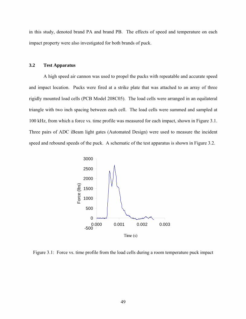
in this study, denoted brand PA and brand PB. The effects of speed and temperature on each
impact property were also investigated for both brands of puck.
3.2 Test Apparatus
A high speed air cannon was used to propel the pucks with repeatable and accurate speed
and impact location. Pucks were fired at a strike plate that was attached to an array of three
rigidly mounted load cells (PCB Model 208C05). The load cells were arranged in an equilateral
triangle with two inch spacing between each cell. The load cells were summed and sampled at
100 kHz, from which a force vs. time profile was measured for each impact, shown in Figure 3.1.
Three pairs of ADC iBeam light gates (Automated Design) were used to measure the incident
speed and rebound speeds of the puck. A schematic of the test apparatus is shown in Figure 3.2.
-500
0
500
1000
1500
2000
2500
3000
0.000 0.001 0.002 0.003
Time (s)
Forc
e (lb
s)
Figure 3.1: Force vs. time profile from the load cells during a room temperature puck impact
49

Figure 3.2: Puck testing schematic
In order to achieve consistent impacts, the puck was propelled in a manner that it was
consistently released on the same trajectory without spin. For this purpose, a sabot was
developed that carried the puck along the barrel of the cannon and released it at the end of the
barrel, illustrated in Figure 3.3. The sabot was made of polyethylene and allowed pucks to be
fired with either a vertical or horizontal orientation.
Figure 3.3: Ice hockey puck sabot
For each impact, the puck was randomly placed into the sabot and the puck/sabot
combination was manually loaded into the cannon. The cannon was fired by opening the valve
to the air accumulator tank using computer control. The puck/sabot traveled down the barrel
Air Cannon Light Gates Rigid Strike Plate
Load Cell Array
50
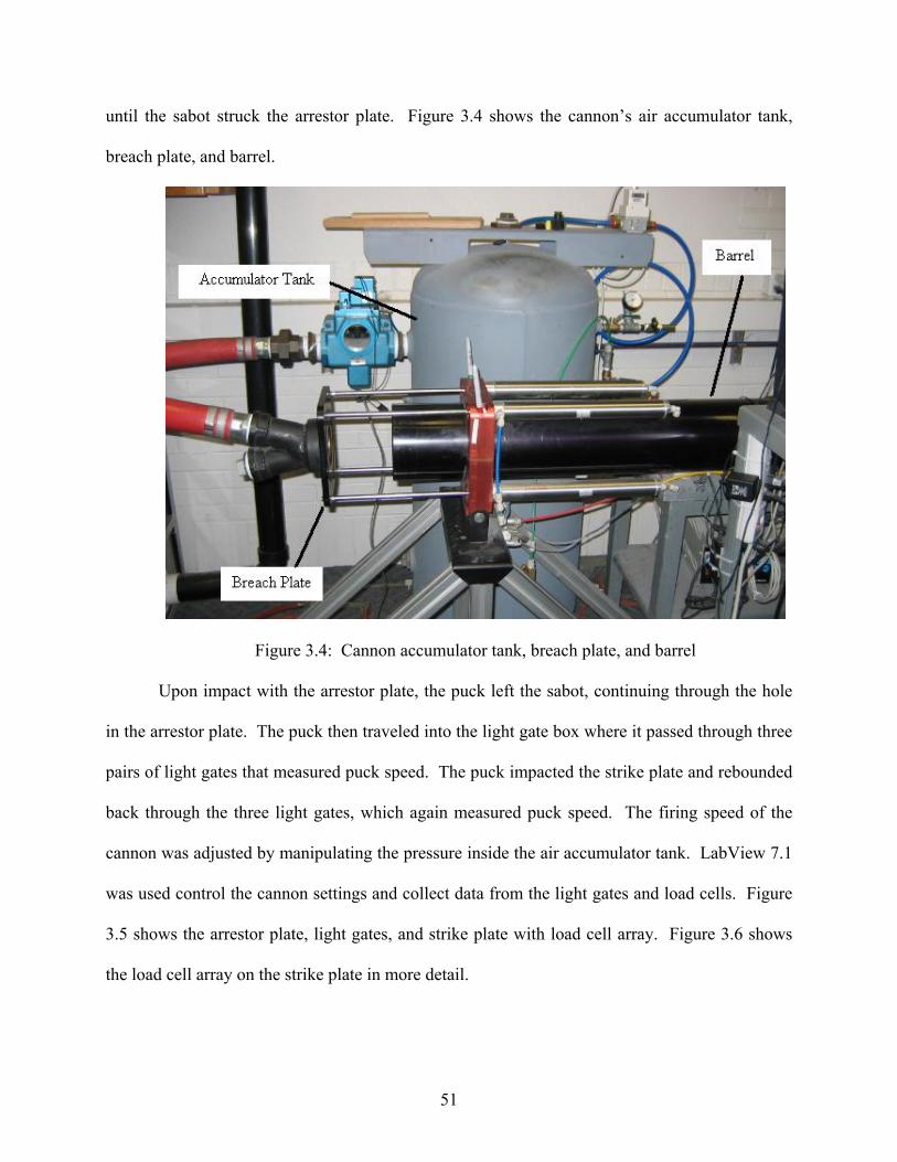
until the sabot struck the arrestor plate. Figure 3.4 shows the cannon’s air accumulator tank,
breach plate, and barrel.
Figure 3.4: Cannon accumulator tank, breach plate, and barrel
Upon impact with the arrestor plate, the puck left the sabot, continuing through the hole
in the arrestor plate. The puck then traveled into the light gate box where it passed through three
pairs of light gates that measured puck speed. The puck impacted the strike plate and rebounded
back through the three light gates, which again measured puck speed. The firing speed of the
cannon was adjusted by manipulating the pressure inside the air accumulator tank. LabView 7.1
was used control the cannon settings and collect data from the light gates and load cells. Figure
3.5 shows the arrestor plate, light gates, and strike plate with load cell array. Figure 3.6 shows
the load cell array on the strike plate in more detail.
51

Figure 3.5: Cannon arrestor plate, light gates, and strike plate
Figure 3.6: Load cell array
During initial puck testing, it was found that the puck was not releasing flatly from the
sabot, and was wobbling on its inbound trajectory. This indicated that there was sufficient slop
in the puck carriage of the sabot to allow it to wobble while riding down the barrel of the cannon.
To alleviate this problem, small cardboard shims were placed inside the sabot to create a tighter
52

fit for the puck. Figure 3.7 shows an illustration of the shims used to stabilize the puck inside the
sabot. In addition, firing the pucks with a vertical orientation reduced wobbling and made the
puck more visible in the high speed video viewframe.
Shims
Figure 3.7: Illustration of shims inside the puck sabot
In all puck testing, a good impact occurred when the puck speed was within 1 mph of the
target, the puck passed through all three light gates without bouncing or wobbling, and impacted
the strike plate. In addition, the rebound was required to pass through all three sets of light gates
at an angle less than 5° from the inbound trajectory without bouncing, wobbling, or spinning.
High speed video and powder spray on the strike plate were used to verify good impacts.
±
Pucks were conditioned to ensure uniform properties for each test. For room temperature
testing, pucks were kept in a controlled environment at 72 ± 2 ° F and relative humidity of 50 ±
5%. For room temperature tests, pucks were impacted twice, then allowed to rest for one hour to
cool down to a uniform temperature. Temperature increases of less than 2° F were noted after
one impact, with the temperature increasing to 75° F or more after two impacts. For frozen tests,
pucks were stored in a controlled freezer. They were impacted once and then underwent a
minimum one hour cool down period in the freezer before further testing. A non-contact infrared
53

temperature sensor was used to verify the temperature of the puck prior to firing. All testing was
conducted in a controlled environment at 72 ± 2 ° F and relative humidity of 50 5%. ±
3.3 Coefficient of Restitution
The coefficient of restitution, or e, was compared for two different brands of pucks that
are made by two different manufacturers. The dependence of e on temperature and speed was
also investigated for both brands of pucks. ASTM 1887 provides a standard test method for
determining e of softballs and baseballs [3.3]. The same method was used in this study. The
coefficient of restitution for each puck was measured by firing the puck at a rigid strike plate and
measuring the inbound and rebound speeds. The value e is then given by Equation (2.2).
Reported e values are averaged from six good impacts for each puck.
For softballs, e decreases linearly with increasing incident velocity [3.4]. Hendee,
Greenwald, and Crisco [3.2] showed a similar linear correlation for baseballs, and found that e
was independent of ball mass. Duris [3.4] and Drane [3.5] have examined the relationship
between softball and baseball temperature and ball coefficient of restitution and found that e
increases nonlinearly with increasing temperature. It is unclear how puck e changes with
temperature and speed.
3.4 Dynamic Stiffness
The dynamic stiffness, or kd provided a measure of the dynamic hardness of pucks. A
proposed ASTM standard provides a method for determining the dynamic stiffness of softballs
and baseballs. The present study employed the same method for finding kd of hockey pucks. In
54

this method, pucks were fired at an array of three load cells. The load cells produced a force vs.
time profile, like the one shown in Figure 3.1.
The dynamic stiffness equation was derived in detail in Chapter 2, section 2.1.2. The
concept of hysteresis, or force-displacement curves was also discussed in the same section. A
sample hysteresis plot for a cricket ball impacting a flat plate at 70 mph is shown in Figure 3.8
below. Testing of softballs and cricket balls has shown a linear loading phase, followed by a
nonlinear restitution phase. Hysteresis curves were generated for each brand of puck, as well as
for different temperatures and impact speeds. Characteristics of hysteresis plots will be
discussed in greater detail in the following sections.
-500
0
500
1000
1500
2000
2500
3000
3500
4000
4500
0.5 0.55 0.6 0.65 0.7 0.75 0.8 0.85
Displacement (in)
Forc
e (lb
s)
Figure 3.8: Sample hysteresis plot for a cricket ball impacting a flat plate
3.5 Test Speed
It is highly desirable to conduct rigid-wall lab testing at speeds that induce response
similar to that seen in actual play. The primary goal is to replicate the amount of deformation of
55
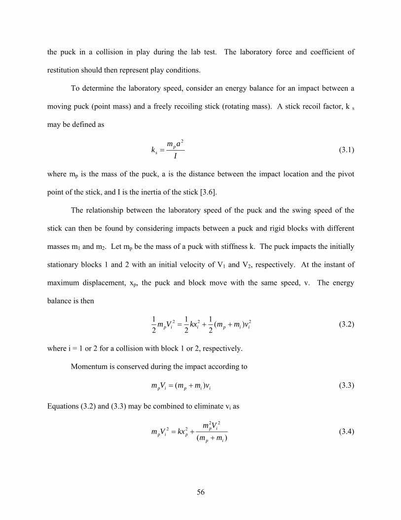
the puck in a collision in play during the lab test. The laboratory force and coefficient of
restitution should then represent play conditions.
To determine the laboratory speed, consider an energy balance for an impact between a
moving puck (point mass) and a freely recoiling stick (rotating mass). A stick recoil factor, k s
may be defined as
Iam
k ps
2
= (3.1)
where mp is the mass of the puck, a is the distance between the impact location and the pivot
point of the stick, and I is the inertia of the stick [3.6].
The relationship between the laboratory speed of the puck and the swing speed of the
stick can then be found by considering impacts between a puck and rigid blocks with different
masses m1 and m2. Let mp be the mass of a puck with stiffness k. The puck impacts the initially
stationary blocks 1 and 2 with an initial velocity of V1 and V2, respectively. At the instant of
maximum displacement, xp, the puck and block move with the same speed, v. The energy
balance is then
222 )(21
21
21
iipiip vmmkxVm ++= (3.2)
where i = 1 or 2 for a collision with block 1 or 2, respectively.
Momentum is conserved during the impact according to
iipip vmmVm )( += (3.3)
Equations (3.2) and (3.3) may be combined to eliminate vi as
)(
2222
ip
ippip mm
VmkxVm
++= (3.4)
56

It is desirable to obtain the same maximum puck deformation, xp in both collisions. Equation
(3.4) may then be evaluated for blocks 1 and 2, and combined to eliminate xp . Solving for the
speed of block 1 gives
2/1
2
121 /1
/1⎟⎟⎠
⎞⎜⎜⎝
⎛
+
+=
mmmm
VVp
p (3.5)
For the case where block 1 is a rigid wall, m1 approaches infinity, so the ratio mp/m1 approaches
zero.
For the case of a swinging object, mi can be viewed as the equivalent swing-weight, or
I/a2 where I is the moment of inertia and a is the distance between the pivot point and the impact
location. Substituting Equation (3.1) into Equation (3.5) and letting V2 be the velocity of the
incoming puck, vp and V1 be the resulting velocity of the stick and puck, Vs gives:
2/1)1( sps kVV += (3.6)
[3.6]. This equation provides a means for calculating the firing speed of a puck, Vp that will
produce the same deformation for known swing speed and ks values. The nominal stick
conditions that were used in developing the stick swing speed formula in Equation (2.21) can be
applied here to get a puck firing speed. That is, for a stick of 10,000 oz-in2 MOI at a pivot
distance of 35 inches that is swinging at 60 mph and a puck weighing 5.8 oz, the equivalent
laboratory speed from solving equation 3.6 is 56.9 mph.
While an ideal test speed for hockey pucks was found to be 56.9 mph, lab and test
restrictions also limit the range of speed that can be used in this study. At speeds below 50 mph,
pucks do not rebound fast enough to pass through all light gates, particularly at lower
temperatures. In addition, at lower temperatures the peak impact force of the puck exceeded the
57

load cell capacity in the test apparatus at speeds above 55 mph. Given these restrictions, a speed
of 55 mph was used for brand comparison and temperature characterization.
3.6 Brand Comparison
Many of the pucks used in play are manufactured by a Canadian company called Viceroy
and distributed under different puck brands. Two brands of pucks made by different
manufacturers that are commonly seen in play were employed in this study. One brand was
produced in Canada and the other in the Czech Republic. The brands will be referred to as brand
PA and brand PB. One dozen of each brand of pucks was tested at 55 mph in this study.
The 55 mph brand comparison showed significant differences in both the coefficient of
restitution and dynamic stiffness for each type of puck. On average, PA pucks were higher in e
by 10.1% and higher in kd by 33.2%. Previous room temperature values for e of hockey pucks
have been found from drop tower tests in the range of e = 0.45 – 0.55 [3.1]. Results here
indicated an average of e = 0.383 for PA and e = 0.349 for PB, both of which are lower than the
results previously found from slow-speed tests.
Average values are summarized in Figure 3.9. Figure 3.10 shows the room temperature
results for dynamic stiffness and e for each puck tested. For the brand comparison at room
temperature, pucks with lower coefficient of restitution also had lower dynamic stiffness. The
differences in both e and kd do not show any overlap of the error bars representing one standard
deviation of the average value. Error bars indicate a stronger difference between kd values than e
in this case.
58
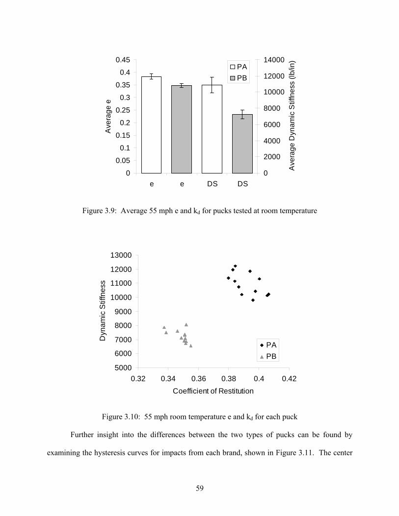
0
0.05
0.1
0.15
0.2
0.25
0.3
0.35
0.4
0.45
e e DS DS
Ave
rage
e
0
2000
4000
6000
8000
10000
12000
14000
Ave
rage
Dyn
amic
Stif
fnes
s (lb
/in)
PAPB
Figure 3.9: Average 55 mph e and kd for pucks tested at room temperature
5000
6000
7000
8000
9000
10000
11000
12000
13000
0.32 0.34 0.36 0.38 0.4 0.42Coefficient of Restitution
Dyn
amic
Stif
fnes
s
PAPB
Figure 3.10: 55 mph room temperature e and kd for each puck
Further insight into the differences between the two types of pucks can be found by
examining the hysteresis curves for impacts from each brand, shown in Figure 3.11. The center
59
of mass displacement was calculated during the contact time for a given impact by solving
Equation (2.10), as previously discussed in section 2.1.2. In each hysteresis curve, a positive
displacement indicates compression of the puck.
A double peak in the force-time and force-displacement curves occurs for both types of
pucks. This double peak can also be seen in Figure 3.1. The double peak is likely due to an
elastic wave traveling in the puck during the contact time. The double peak is not due to tooling
of the test fixture, as the post-impact vibration is small. It is suspected that the wave travels in
the transverse direction, or through the thickness of the puck. Because pucks are roughly three
times larger in diameter than they are thick, a wave in the transverse direction would travel three
times faster than a wave across the diameter of the puck. This provides a reasonable explanation
for the double-peak observed in these tests. For brand PA, the first peak was always higher than
the second peak, while the opposite was true for all impacts with brand PB at room temperature.
For both brands, the loading phase was essentially linear up to the first peak
displacement, while the unloading phase was nonlinear. The slope of the loading phase on the
hysteresis curves was also different between the two brands of pucks, with brand PA having a
steeper slope. The brand PA puck used in this comparison reached a peak force that was 20%
higher than the brand PB puck. Brand PB peak displacement was 9% higher than brand PA for
the comparison between the two impacts shown in Figure 3.11. Similar results were found when
comparing other pucks from the two brands.
60
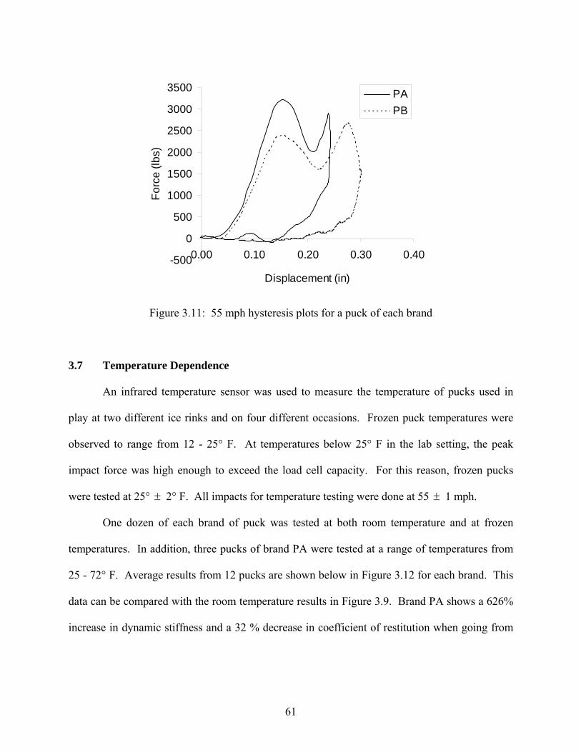
-500
0
500
1000
1500
2000
2500
3000
3500
0.00 0.10 0.20 0.30 0.40
Displacement (in)
Forc
e (lb
s)
PAPB
Figure 3.11: 55 mph hysteresis plots for a puck of each brand
3.7 Temperature Dependence
An infrared temperature sensor was used to measure the temperature of pucks used in
play at two different ice rinks and on four different occasions. Frozen puck temperatures were
observed to range from 12 - 25° F. At temperatures below 25° F in the lab setting, the peak
impact force was high enough to exceed the load cell capacity. For this reason, frozen pucks
were tested at 25° 2° F. All impacts for temperature testing were done at 55 1 mph. ± ±
One dozen of each brand of puck was tested at both room temperature and at frozen
temperatures. In addition, three pucks of brand PA were tested at a range of temperatures from
25 - 72° F. Average results from 12 pucks are shown below in Figure 3.12 for each brand. This
data can be compared with the room temperature results in Figure 3.9. Brand PA shows a 626%
increase in dynamic stiffness and a 32 % decrease in coefficient of restitution when going from
61

72° to 25° F. Similarly, brand PB showed a 488 % increase in dynamic stiffness and a 26 %
decrease in coefficient of restitution over the same temperature range.
At room temperature the brands had error bars representing one standard deviation of e
that did not overlap, but at frozen temperatures the error bars do overlap, suggesting that
differences in e became less significant at lower temperatures. Drop tower tests found frozen e
values in the range of 0.12 – 0.27 [3.1]. Averages found here were e = 0.267 for PA and e =
0.256 for PB, which are within the range previously found from slow speed tests.
0
0.05
0.1
0.15
0.2
0.25
0.3
e e DS DS
Ave
rage
e
0
10000
20000
30000
40000
50000
60000
70000
80000
90000
Ave
rage
Dyn
amic
Stif
fnes
s (lb
/in)PA
PB
Figure 3.12: Average 55 mph e and kd for pucks tested at 25° F
Figure 3.13 shows the results for each puck at room temperature (72° F) and frozen (25°
F). Brand PA underwent larger changes in impact properties than brand PB for the same
temperature interval. For both the frozen and the room temperature cases, brand PB had lower
dynamic stiffness and coefficient of restitution than brand PA.
62

0
10000
20000
30000
40000
50000
60000
70000
80000
90000
0.23 0.28 0.33 0.38Coefficient of Restitution
Dyn
amic
Stif
fnes
s (lb
/in) PA 25 F
PB 25 FPA 72 FPB 72 F
Figure 3.13: 55 mph room temperature and frozen results for each puck
Three pucks of brand PA were tested at a range of temperatures between 25° to 72° F.
Results of this temperature characterization are shown in Figure 3.14. As expected, the
coefficient of restitution decreases with decreasing temperature, while the dynamic stiffness
increases with decreasing temperature. Both changes are nonlinear. It is interesting to note that
the coefficient of restitution appears to plateau at lower temperatures, while the dynamic stiffness
appears to plateau at higher temperatures.
63
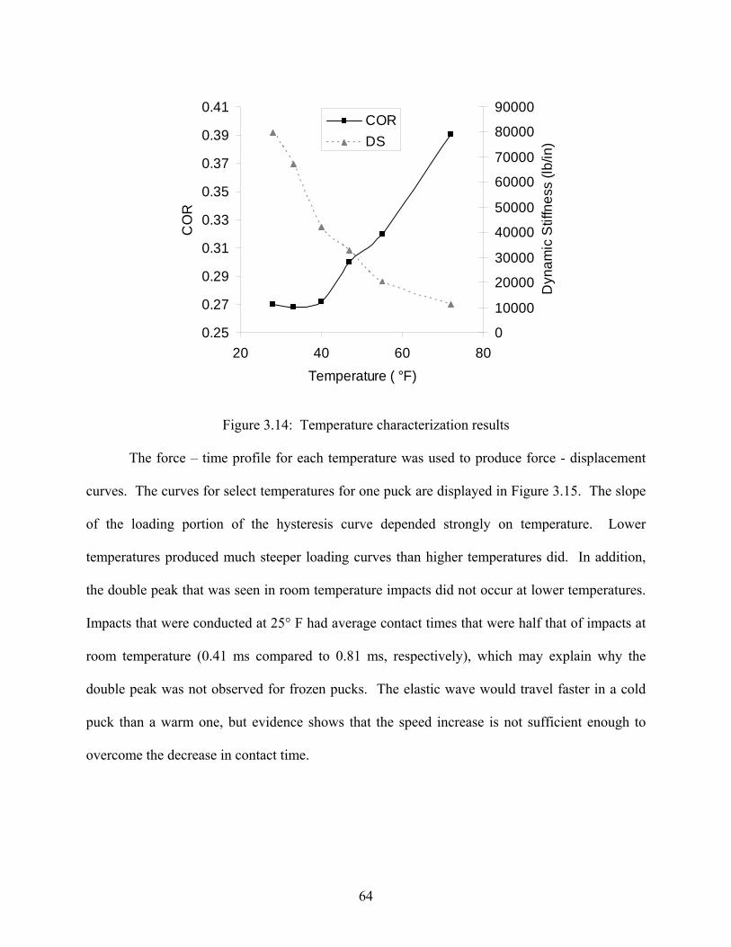
0.25
0.27
0.29
0.31
0.33
0.35
0.37
0.39
0.41
20 40 60 80Temperature ( °F)
CO
R
0
10000
20000
30000
40000
50000
60000
70000
80000
90000
Dyn
amic
Stif
fnes
s (lb
/in)
CORDS
Figure 3.14: Temperature characterization results
The force – time profile for each temperature was used to produce force - displacement
curves. The curves for select temperatures for one puck are displayed in Figure 3.15. The slope
of the loading portion of the hysteresis curve depended strongly on temperature. Lower
temperatures produced much steeper loading curves than higher temperatures did. In addition,
the double peak that was seen in room temperature impacts did not occur at lower temperatures.
Impacts that were conducted at 25° F had average contact times that were half that of impacts at
room temperature (0.41 ms compared to 0.81 ms, respectively), which may explain why the
double peak was not observed for frozen pucks. The elastic wave would travel faster in a cold
puck than a warm one, but evidence shows that the speed increase is not sufficient enough to
overcome the decrease in contact time.
64
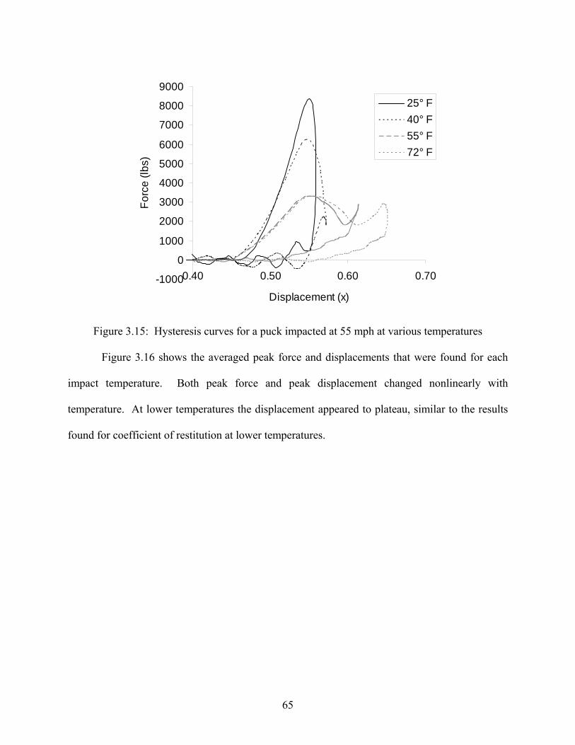
-1000
0
1000
2000
3000
4000
5000
6000
7000
8000
9000
0.40 0.50 0.60 0.70
Displacement (x)
Forc
e (lb
s)
25° F40° F55° F72° F
Figure 3.15: Hysteresis curves for a puck impacted at 55 mph at various temperatures
Figure 3.16 shows the averaged peak force and displacements that were found for each
impact temperature. Both peak force and peak displacement changed nonlinearly with
temperature. At lower temperatures the displacement appeared to plateau, similar to the results
found for coefficient of restitution at lower temperatures.
65

0
1000
2000
3000
4000
5000
6000
7000
8000
9000
20 40 60 80Puck Temperature (°F)
Ave
rage
Pea
k Fo
rce
(lbs)
0.54
0.56
0.58
0.60
0.62
0.64
0.66
Ave
rage
Pea
k D
ispl
acem
ent (
in)
ForceDisplacement
Figure 3.16: Peak force and displacement for pucks impacted at 55 mph at various temperatures
3.8 Rate Dependence
The response of viscoelastic materials depends on the applied strain rate [3.7]. While the
term rate dependence typically refers to the rate of loading, this study is more concerned with
how e and kd change with impact speed. Furthermore, rate dependence in this study refers to the
speed of the impact for PA brand pucks. Golf balls, softballs, baseballs, and cricket balls have
all been shown to have varying degrees of rate dependence [3.8]. The rate dependence of hockey
pucks has not been previously studied.
Brand PA pucks were tested for rate dependence at room temperature (72 ± 2°F). Impact
speeds ranged from 55 1 mph to 85 ± ± 1 mph in 10 mph intervals. Figure 3.17 shows how the
dynamic stiffness and coefficient of restitution varied with impact speed. The coefficient of
restitution decreased linearly with increasing speed. Drop test results [3.1] have been included
66
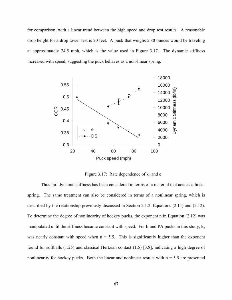
for comparison, with a linear trend between the high speed and drop test results. A reasonable
drop height for a drop tower test is 20 feet. A puck that weighs 5.80 ounces would be traveling
at approximately 24.5 mph, which is the value used in Figure 3.17. The dynamic stiffness
increased with speed, suggesting the puck behaves as a non-linear spring.
0.3
0.35
0.4
0.45
0.5
0.55
20 40 60 80 100Puck speed (mph)
CO
R
0
2000
4000
6000
8000
10000
12000
14000
16000
18000
Dyn
amic
Stif
fnes
s (lb
/in)
eDS
Figure 3.17: Rate dependence of kd and e
Thus far, dynamic stiffness has been considered in terms of a material that acts as a linear
spring. The same treatment can also be considered in terms of a nonlinear spring, which is
described by the relationship previously discussed in Section 2.1.2, Equations (2.11) and (2.12).
To determine the degree of nonlinearity of hockey pucks, the exponent n in Equation (2.12) was
manipulated until the stiffness became constant with speed. For brand PA pucks in this study, kn
was nearly constant with speed when n = 5.5. This is significantly higher than the exponent
found for softballs (1.25) and classical Hertzian contact (1.5) [3.8], indicating a high degree of
nonlinearity for hockey pucks. Both the linear and nonlinear results with n = 5.5 are presented
67
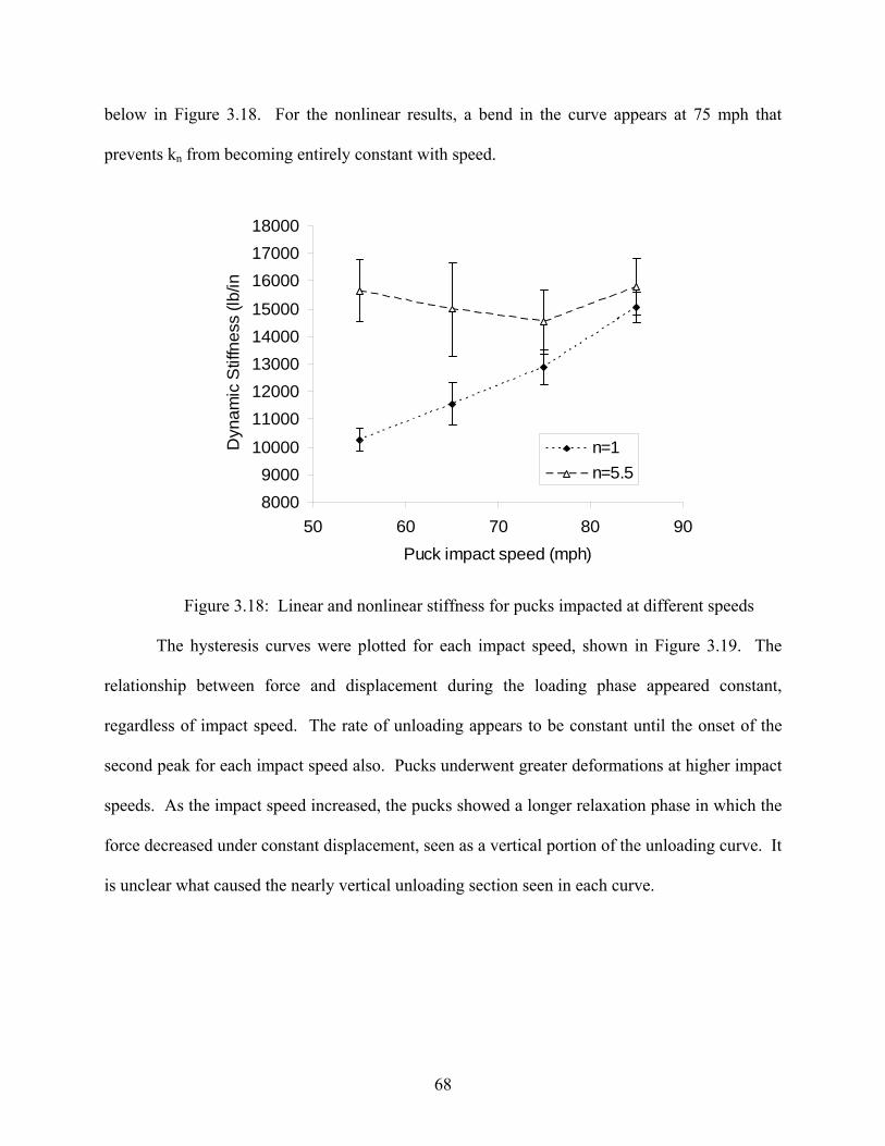
below in Figure 3.18. For the nonlinear results, a bend in the curve appears at 75 mph that
prevents kn from becoming entirely constant with speed.
80009000
10000
1100012000130001400015000
160001700018000
50 60 70 80 90Puck impact speed (mph)
Dyn
amic
Stif
fnes
s (lb
/in
n=1n=5.5
Figure 3.18: Linear and nonlinear stiffness for pucks impacted at different speeds
The hysteresis curves were plotted for each impact speed, shown in Figure 3.19. The
relationship between force and displacement during the loading phase appeared constant,
regardless of impact speed. The rate of unloading appears to be constant until the onset of the
second peak for each impact speed also. Pucks underwent greater deformations at higher impact
speeds. As the impact speed increased, the pucks showed a longer relaxation phase in which the
force decreased under constant displacement, seen as a vertical portion of the unloading curve. It
is unclear what caused the nearly vertical unloading section seen in each curve.
68
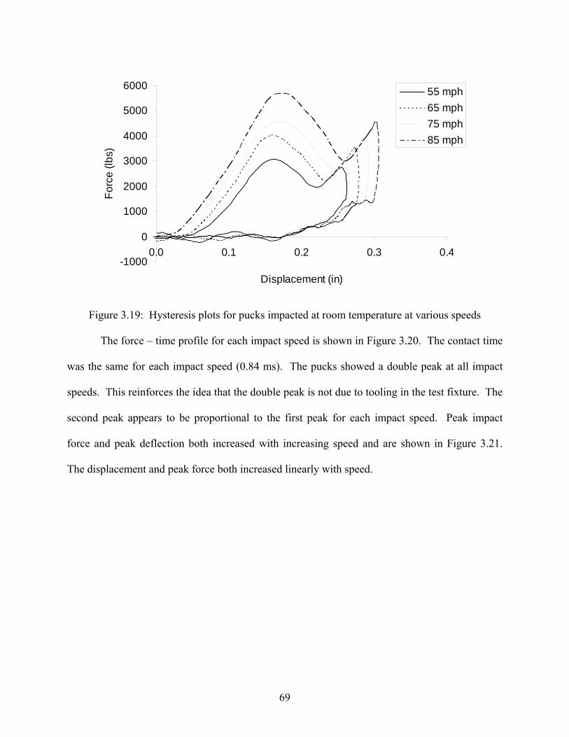
-1000
0
1000
2000
3000
4000
5000
6000
0.0 0.1 0.2 0.3 0.4
Displacement (in)
Forc
e (lb
s)55 mph65 mph75 mph85 mph
Figure 3.19: Hysteresis plots for pucks impacted at room temperature at various speeds
The force – time profile for each impact speed is shown in Figure 3.20. The contact time
was the same for each impact speed (0.84 ms). The pucks showed a double peak at all impact
speeds. This reinforces the idea that the double peak is not due to tooling in the test fixture. The
second peak appears to be proportional to the first peak for each impact speed. Peak impact
force and peak deflection both increased with increasing speed and are shown in Figure 3.21.
The displacement and peak force both increased linearly with speed.
69

-20000
2000400060008000
100001200014000160001800020000
0.24
0.33
0.42
0.51
0.60
0.69
0.78
0.87
0.96
1.05
1.14
1.23
1.32
1.41
Time (ms)
Forc
e (lb
s)
85 mph75 mph65 mph55 mph
Figure 3.20: Force – time profile for each puck impact speed at room temperature
0
1000
2000
3000
4000
5000
6000
50 60 70 80 90Puck Impact Speed (mph)
Ave
rage
Pea
k Fo
rce
(lbs)
0.4
0.6
0.8
1.0
1.2
Ave
rage
Pea
k D
ispl
acem
ent
(in)
ForceDisplacement
Figure 3.21: Peak force and displacement for pucks impacted at various speeds
70

3.9 Quasi-Static Stiffness
Softballs are characterized according to their quasi-static compression, described by
ASTM F1888-04 [3.10]. To determine the difference between quasi-static and dynamic puck
stiffness, pucks were compressed quasi-statically using the same procedure at room temperature.
Pucks were placed between two flat plates in a load frame (MTS Systems Corporation, Eden
Prairie, MN), shown in Figure 3.22. A preload of 4 ± 1 pounds was first applied to the puck.
The puck was then compressed 0.25 inches over a 15 second time period and the maximum force
was recorded. The puck was then rotated 90° in the radial direction and compressed again. The
reported stiffness value for each puck was the average stiffness from the two locations.
Figure 3.22: Quasi-static puck compression testing setup
Average compression results for the 12 pucks of each brand are presented in Figure 3.23.
Dynamic stiffness results at 72° F are also included for comparison. As expected, the dynamic
stiffness is much larger than the quasi-static stiffness due to the larger impact force that is
exerted by a faster traveling puck in the dynamic case. Brand PA pucks were 49.4% stiffer than
PB pucks when stiffness was measured quasi-statically. This is a larger difference than was seen
71
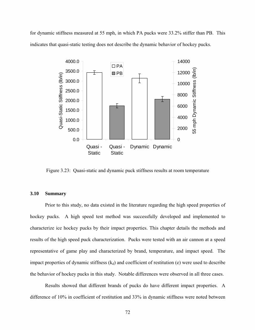
for dynamic stiffness measured at 55 mph, in which PA pucks were 33.2% stiffer than PB. This
indicates that quasi-static testing does not describe the dynamic behavior of hockey pucks.
0.0
500.0
1000.0
1500.0
2000.0
2500.0
3000.0
3500.0
4000.0
Quasi -Static
Quasi -Static
Dynamic Dynamic
Qua
si-S
tatic
Stif
fnes
s (lb
/in)
0
2000
4000
6000
8000
10000
12000
14000
55 m
ph D
ynam
ic S
tiffn
ess
(lb/in
)PAPB
Figure 3.23: Quasi-static and dynamic puck stiffness results at room temperature
3.10 Summary
Prior to this study, no data existed in the literature regarding the high speed properties of
hockey pucks. A high speed test method was successfully developed and implemented to
characterize ice hockey pucks by their impact properties. This chapter details the methods and
results of the high speed puck characterization. Pucks were tested with an air cannon at a speed
representative of game play and characterized by brand, temperature, and impact speed. The
impact properties of dynamic stiffness (kd) and coefficient of restitution (e) were used to describe
the behavior of hockey pucks in this study. Notable differences were observed in all three cases.
Results showed that different brands of pucks do have different impact properties. A
difference of 10% in coefficient of restitution and 33% in dynamic stiffness were noted between
72
two brands. In addition, a difference of 20% in the peak force and 9% in peak deflection were
found. These results indicate that measurable differences in puck properties do exist from one
brand to another which is not apparent by physical examination. It is possible that these
differences were noted in the large ranges observed in e for drop tower tests.
Pucks were tested at a variety of temperatures ranging from 25° – 72° F and at 55 ± 1
mph. The behavior of both brands of pucks appeared to be highly dependent on temperature. In
general, e increased with increasing temperature (by 32% and 26%) while kd decreased
drastically with increasing temperature (626% and 488%). Freezing pucks before play makes
them significantly stiffer and less elastic, therefore improving the controllability for players.
Freezing pucks decreased the contact time of the collision. On average, the contact time
at 25° F was half that at 72° F. This is a likely explanation for why the double peak from an
elastic wave in the puck was not seen at low temperatures. Examination of the hysteresis curves
showed that the puck temperature has a significant effect on the relationship between force and
displacement for both the loading and unloading phases. Peak deflection increased nonlinearly
with increasing temperature.
Pucks were tested at room temperature (72 ± 2° F) at speeds ranging from 55 – 85 mph
in 10 mph intervals. The coefficient of restitution was shown to decrease while the dynamic
stiffness increased with increasing impact speed. Significant changes were observed, showing
that quasi-static testing (like drop tower tests) may not be indicative of dynamic behavior. The
increase in dynamic stiffness with speed indicates that hockey pucks are more nonlinear than
softballs. The contact time of the collision was shown to be constant for changing impact speed.
The peak displacement and peak force both increased linearly with increasing speed. Quasi-
static stiffness testing showed larger differences between the two brands than the stiffness values
73
that were found at 55 mph. In addition, puck impact properties appear to be more dependent on
temperature than speed, as multiple differences were observed in temperature tests that were not
seen in speed testing.
74
REFERENCES
[3.1] Hache, A., The Physics of Ice Hockey. The Johns Hopkins University Press, Baltimore and London, 2002.
[3.2] Hendee, S.P., Greenwald, R.M., Crisco, J.J. Static and Dynamic Properties of Various
Baseballs. J. App. Biomech. 14, p. 390-400 (1998). [3.3] ASTM F1887 Standard Test Method for Measuring the Coefficient of Restitution (COR)
of Baseballs and Softballs, ASTM International 2004. [3.4] Duris, J.G., Eperimental and numerical characterization of softballs, Master’s Thesis,
Washington State University, 2004. [3.5] Drane, P.J. and Sherwood, J.A., Characterization of the effect of temperature on baseball
COR performance, Proceedings from the Eng. of Sport 5 (2), p. 59-65. 2004. [3.6] Smith, L.V., Measuring the Hardness of Softballs, Proceedings of the XXIV International
Conference on Modal Analysis, Orlando (2008). [3.7] Gibson, R.F., Principles of Composite Materials Mechanics, Second Ed., CRC Press,
Boca Raton, FL, 2007. ISBN: 0-8247-5389-5. [3.8] Smith, L.V., Duris, J.G., and Nathan, A.M., Describing the Dynamic Response of
Softballs, Society of Experimental Mechanics, submitted August 2007. [3.9] Stronge, William James, Impact Mechanics. Cambridge University Press, Cambridge,
United Kingdom (2000). ISBN 0-521-63286-2. [3.10] ASTM F1888-04 Standard Test Method for Compression-Displacement of Baseballs and
Softballs, ASTM International, Pennsylvania (2004).
75
CHAPTER FOUR
EXPERIMENTAL STICK RESULTS
4.1 Introduction
The ice hockey stick market has been rapidly evolving in recent years. New materials
and features have been introduced to hockey sticks, but the effects of these modifications on the
performance of the stick are not currently understood. Previous studies regarding the
performance and mechanics of ice hockey sticks and shots have mainly concentrated on
identifying player movement patterns that are important in developing a good shot, regardless of
the stick type being used [4.1, 4.2, 4.3].
The following compares laboratory measures of stick performance. A performance test
using a high speed cannon was developed and implemented to test different types of sticks in
terms of a modeled slap shot. Modal analysis was used to investigate the vibration
characteristics of hockey sticks, with the hope of gaining some insight into player feel. Finally,
lab performance data was compared to slap shots seen in the field of play.
Two main stick variables were investigated in this study: stick material and shaft taper.
The sticks used in this study were classified by their material with a W# corresponding to a wood
stick and a C# corresponding to a composite stick. Furthermore, sticks were classified by the
amount of taper in the shaft. Sticks with no taper were classified as straight-shaft composite.
Intermediate tapered sticks indicate some tapering in the shaft, and long tapered elite sticks that
are among the best sticks on the market, reportedly with the longest shaft tapers of any sticks
currently available. Seventeen hockey sticks were compared in this study, including 6 wood and
76

11 composite sticks. They were a selection from four different hockey stick manufacturers. The
sticks are summarized in Table 4.1.
Table 4.1: Summary of sticks tested
Stick Number Material Geometry W1 Wood Straight shaft W2 Wood Straight shaft W3 Wood Straight shaft W4 Wood with composite blade Straight shaft W5 Wood Tapered shaft W6 Wood with composite blade Tapered shaft C1 Composite Straight shaft C2 Composite Straight shaft C3 Composite Tapered shaft - low C4 Composite Tapered shaft - mid C5 Composite Tapered shaft - mid C6 Composite Tapered shaft - mid/high C7 Composite Tapered shaft - high C8 Composite Elite composite C9 Composite Elite composite C10 Composite Elite composite C11 Composite Elite composite
4.2 Modal Analysis
One of the primary player concerns when choosing a hockey stick is the perceived feel of
the stick. Players want to be able to feel small impacts between the stick and the puck due to
handling so they have some perception of where the puck is in relation to the stick without
having to look down. In addition, feel is important in catching a pass with the stick. If a player
cannot feel the puck impacting the stick, it is harder to cushion the pass, often sending the puck
careening away from the player.
The analysis of feel is complicated by its highly subjective nature [4.15]. It was hoped
that modal analysis could be used to characterize stick vibration, offering some insight into the
issue of perceived feel of a stick. Mode shapes, modal frequencies, and damping were compared
77
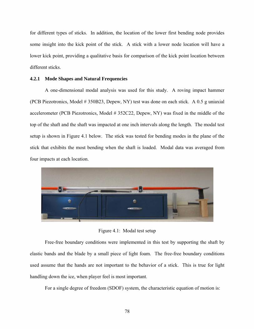
for different types of sticks. In addition, the location of the lower first bending node provides
some insight into the kick point of the stick. A stick with a lower node location will have a
lower kick point, providing a qualitative basis for comparison of the kick point location between
different sticks.
4.2.1 Mode Shapes and Natural Frequencies
A one-dimensional modal analysis was used for this study. A roving impact hammer
(PCB Piezotronics, Model # 350B23, Depew, NY) test was done on each stick. A 0.5 g uniaxial
accelerometer (PCB Piezotronics, Model # 352C22, Depew, NY) was fixed in the middle of the
top of the shaft and the shaft was impacted at one inch intervals along the length. The modal test
setup is shown in Figure 4.1 below. The stick was tested for bending modes in the plane of the
stick that exhibits the most bending when the shaft is loaded. Modal data was averaged from
four impacts at each location.
Figure 4.1: Modal test setup
Free-free boundary conditions were implemented in this test by supporting the shaft by
elastic bands and the blade by a small piece of light foam. The free-free boundary conditions
used assume that the hands are not important to the behavior of a stick. This is true for light
handling down the ice, when player feel is most important.
For a single degree of freedom (SDOF) system, the characteristic equation of motion is:
78
)(tfkxxcxm =++ &&& (4.1)
where m is the mass, c is the damping coefficient, k is the spring stiffness, and f(t) is the sum of
the applied forces as a function of time. The displacement of the system is x and each dot
represents a time derivative of displacement. Vibration consists of a combination of inertial,
damping, spring, and excitation forces.
The Frequency Response Function (FRF) describes the input-output relationship between
two points on a structure as a function of frequency. It is defined as [4.13]:
)()(
InputFFTOutputFFTFRF = (4.2)
where the FFT is the Fast Fourier Transform of the input or output function. The FRF is a
complex function with both real and imaginary parts that relates the output per unit of input for
each frequency. Peaks occur in the FRF at resonant or natural frequencies where the time
response was observed to have maximum response corresponding to the rate of oscillation of the
input excitation [4.13]. The amplitude of the peak describes the mode shape, while the steepness
of the peak in the time domain describes the damping of that mode.
The method of quadrature picking was used to analyze modal data and extract mode
shapes and natural frequencies. This method involves plotting the imaginary part of the FRF as a
function of position along the length of the stick. The resulting three-dimensional plot is referred
to as a waterfall plot. A sample waterfall plot is shown in Chapter 2, Figure 2.6 and another is
shown in Figure 4.2. The waterfall plot shows the various mode shapes along the length of the
stick.
In this study, a one-dimensional bending analysis was performed on each hockey stick.
In reality, the vibration of a hockey stick is more complex. The blade acted as a point mass that
oscillated in torsion around the shaft, causing more complex vibration patterns. Torsional modes
79

appeared as mirrors of bending modes at frequencies higher than the second bending mode
natural frequency. Figure 4.2 shows the first torsional mode appearing as a mirror of the third
bending mode for a composite hockey stick.
Figure 4.2: Waterfall plot with torsional mode appearing as mirror of bending mode
More robust analysis techniques were needed to distinguish between torsional and
bending modes, which were outside the scope of this study. One mid-tapered composite hockey
stick was sent to Dr. Dan Russell at Kettering University for further analysis. By conducting a
two-dimensional modal analysis and using more complex analysis software, he was able to
determine which modes were bending and torsional modes. The accelerometer was fixed to the
blade of the stick a total of 213 impact locations on the handle and blade were used. Dr.
Russell’s modal setup is shown in Figure 4.3 and the resulting modal frequencies up through
1000 Hz in Table 4.2.
80

Figure 4.3: Dr. Dan Russell’s 2-dimensional modal analysis setup
Table 4.2: Summary of modal frequencies found by Dr. Dan Russell
Frequency (Hz) Mode Shape 56 First Bending
144 Second Bending 243 First Torsional 284 Third Bending 424 Fourth Bending 478 Second Torsional 575 Fifth Bending 749 Sixth Bending 966 Seventh Bending
The remainder of the modal comparison focused on the first two bending modes for each
of the 16 sticks tested. Also of interest was the location of the first bending node. The location
provided some insight into the location of the kick point of the stick. Knowing the location of
the lower first bending node allows for qualitative comparison of the kick point location between
different hockey sticks.
81

Results showed that natural frequencies for modes 1 and 2 were fairly similar for all
sticks. Mode 1 ranged from 46 – 60 Hz, while mode 2 showed a wider range, from 111 – 161
Hz. All of the wood sticks had lower natural frequencies than the composite sticks. Wood sticks
are reported to offer a better feel for the puck than composite, but no drastic difference between
the first two bending modes for wood and composite sticks was seen. Mode 1 and 2 frequencies
are shown in Figure 4.4 for all sticks.
0
20
40
60
80
100
120
140
160
180
W1
W2
W3
W4
W5
W6
C1
C2
C3
C4
C5
C6
C7
C8
C9
C10
C11
Stick Number
Freq
uenc
y (H
z)
Mode 1Mode 2
Figure 4.4: Mode 1 and 2 natural frequencies for all sticks
It is postulated here that higher frequencies may contribute more to the player’s
perception of feel. Examining higher modal frequencies was determined to be outside the scope
of this study. Hocknell, et al. [4.15] compared the subjective feel and vibration characteristics
for wood and aluminum golf club shafts. They found that vibration in the range of 0 – 2.5 kHz
was believed to be of greater importance to the sensation in the golfer’s hands. They concluded
that desirable sensation in the hands can be achieved by exciting modes of vibration in the
82

frequency range of 500 Hz – 2.5 kHz more strongly than modes in the region of 100 Hz. It is
unclear at this time how a hockey player’s thick leather gloves would affect perception of
vibrations in these ranges.
Each bending mode, m has m + 1 nodes, meaning that mode 1 has two nodes. The nodes
are shown below in Figure 4.5, which contains a plot of the first two bending modes for stick C5.
The 0 inch location corresponds to the bottom of the hosel, where the blade ends and the shaft
begins. An array was created with the imaginary part of the FRF for each impact location along
the length of the stick. The natural frequencies were then identified and the FRF value
(amplitude) for each impact location at that frequency was plotted. The natural frequencies are
identified in the legend of the plot. The nodes are the location in which the mode shape has zero
amplitude. Locations on the stick were measured up from the bottom of the shaft, where the heel
of the blade begins to curve. Of particular interest in this study was the location of the lower first
bending node. The The lower node location is shown in Figure 4.6 for each stick.
-10
-8
-6
-4
-2
0
2
4
6
8
10
0 10 20 30 40 50 60
Stick Location (in)
Am
plitu
de (d
B)
153 Hz50 Hz
Figure 4.5: Bending modes 1 and 2 for stick C5
83
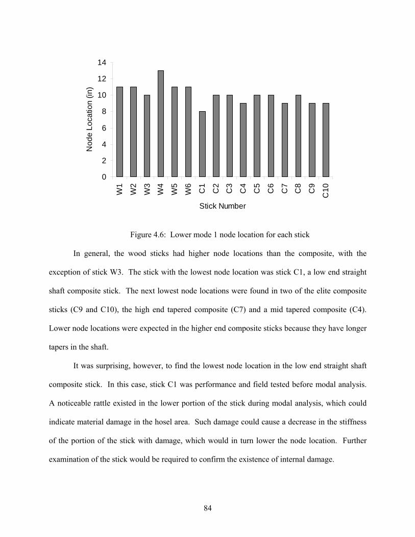
0
2
4
6
8
10
12
14
W1
W2
W3
W4
W5
W6
C1
C2
C3
C4
C5
C6
C7
C8
C9
C10
Stick Number
Nod
e Lo
catio
n (in
)
Figure 4.6: Lower mode 1 node location for each stick
In general, the wood sticks had higher node locations than the composite, with the
exception of stick W3. The stick with the lowest node location was stick C1, a low end straight
shaft composite stick. The next lowest node locations were found in two of the elite composite
sticks (C9 and C10), the high end tapered composite (C7) and a mid tapered composite (C4).
Lower node locations were expected in the higher end composite sticks because they have longer
tapers in the shaft.
It was surprising, however, to find the lowest node location in the low end straight shaft
composite stick. In this case, stick C1 was performance and field tested before modal analysis.
A noticeable rattle existed in the lower portion of the stick during modal analysis, which could
indicate material damage in the hosel area. Such damage could cause a decrease in the stiffness
of the portion of the stick with damage, which would in turn lower the node location. Further
examination of the stick would be required to confirm the existence of internal damage.
84
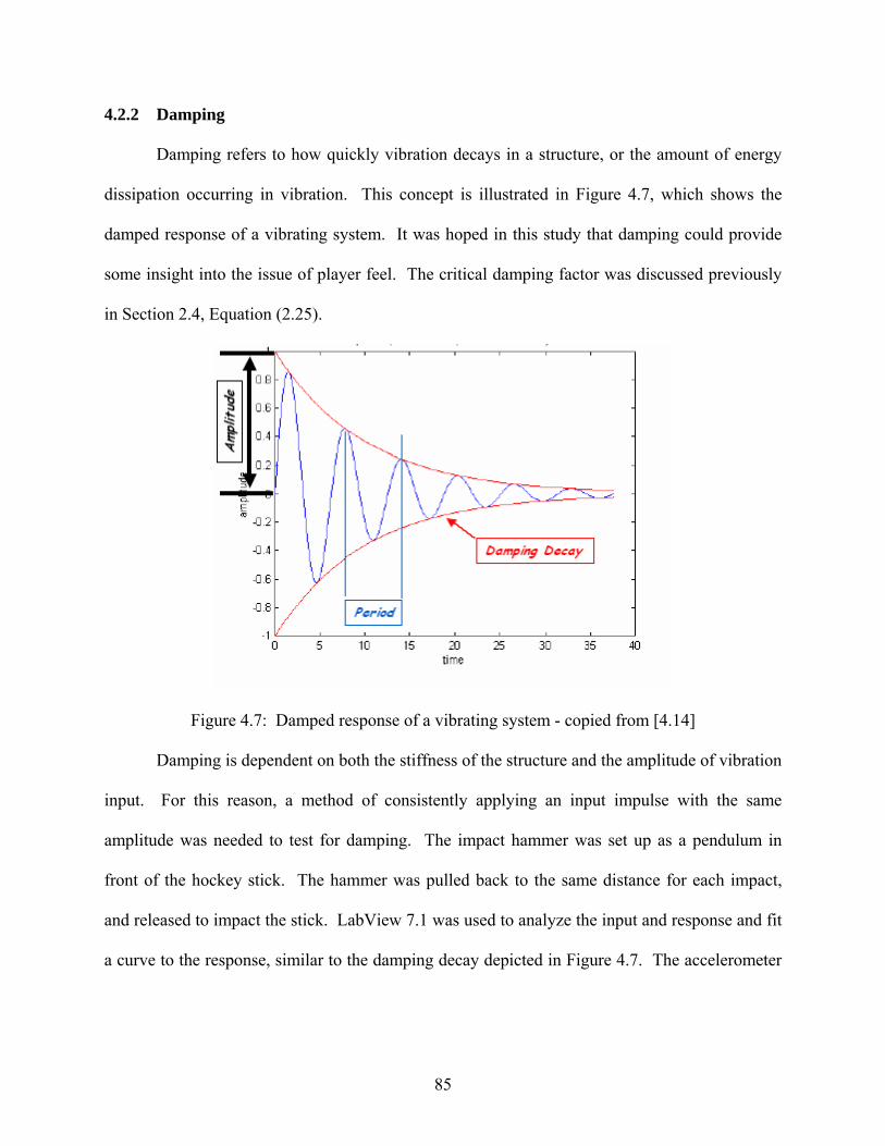
4.2.2 Damping
Damping refers to how quickly vibration decays in a structure, or the amount of energy
dissipation occurring in vibration. This concept is illustrated in Figure 4.7, which shows the
damped response of a vibrating system. It was hoped in this study that damping could provide
some insight into the issue of player feel. The critical damping factor was discussed previously
in Section 2.4, Equation (2.25).
Figure 4.7: Damped response of a vibrating system - copied from [4.14]
Damping is dependent on both the stiffness of the structure and the amplitude of vibration
input. For this reason, a method of consistently applying an input impulse with the same
amplitude was needed to test for damping. The impact hammer was set up as a pendulum in
front of the hockey stick. The hammer was pulled back to the same distance for each impact,
and released to impact the stick. LabView 7.1 was used to analyze the input and response and fit
a curve to the response, similar to the damping decay depicted in Figure 4.7. The accelerometer
85
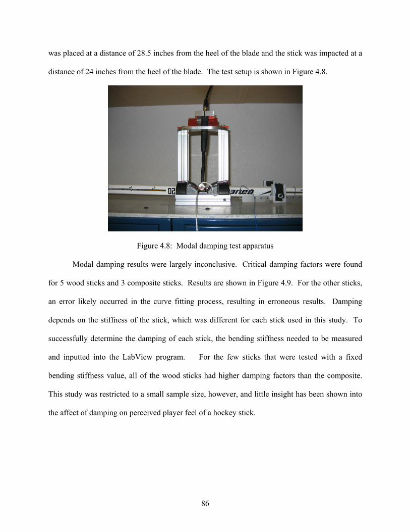
was placed at a distance of 28.5 inches from the heel of the blade and the stick was impacted at a
distance of 24 inches from the heel of the blade. The test setup is shown in Figure 4.8.
Figure 4.8: Modal damping test apparatus
Modal damping results were largely inconclusive. Critical damping factors were found
for 5 wood sticks and 3 composite sticks. Results are shown in Figure 4.9. For the other sticks,
an error likely occurred in the curve fitting process, resulting in erroneous results. Damping
depends on the stiffness of the stick, which was different for each stick used in this study. To
successfully determine the damping of each stick, the bending stiffness needed to be measured
and inputted into the LabView program. For the few sticks that were tested with a fixed
bending stiffness value, all of the wood sticks had higher damping factors than the composite.
This study was restricted to a small sample size, however, and little insight has been shown into
the affect of damping on perceived player feel of a hockey stick.
86

00.0005
0.0010.0015
0.0020.0025
0.0030.0035
0.0040.0045
0.005
W2 W3 W4 W5 W6 C6 C7 C11Stick Number
Crit
ical
Dam
ping
Fac
tor
Figure 4.9: Critical damping factor for 8 sticks
4.3 Field Study
A field study was conducted that utilized three players shooting pucks with various sticks
on ice. The primary goals of this field study were to determine stick swing speeds seen in actual
play and to correlate lab performance to data taken from actual play. Correlation between lab
performance data and field study is presented in section 4.4.8 below, while speed findings are
presented here. Subjects used six different hockey sticks to perform stationary slap shots on the
ice toward a net. A high speed video camera (Photron FASTCAM 1024 PCI) was used to
capture the stationary slap shots at 1000 frames/second while a radar gun (JUGS INC.) was used
to measure resulting puck speeds.
The field study was conducted at the Rotary Veteran’s Memorial Pavilion Ice Rink in
Moscow, Idaho. Subjects utilized in this study were three local recreational hockey players. Six
sticks were selected for subjects to shoot with: a wood stick, a straight shaft composite stick, a
low-end tapered shaft composite stick, an intermediate tapered stick, and two long tapered elite
87

composite sticks. Subjects completed a minimum number of ten stationary slap shots with each
stick. Sticks were selected in random order for each subject. Acceptable slap shots were those
in which the subject indicated maximum effort, expressed satisfaction with the quality of the
shot, and in which the puck hit the net.
Six sticks from the overall study were selected for use in the field study and are
summarized below in Table 4.3. The selection of sticks represented a good survey of stick types
currently available on the market. Five of the sticks were composite, ranging from low end
straight-shaft to elite tapered, and the sixth stick was wood. The wood stick broke early in the
study before any usable high speed video was collected. The “sister” designation after sticks
C11 and W1 indicates that these sticks broke before a full performance scan was completed, and
another stick of the same model was used in the performance testing and modal analysis.
Table 4.3: Summary of sticks used in the field study
Stick Number Stick Type C11 sister Elite tapered composite
C8 Elite tapered composite C2 Low end tapered composite C1 Low end straight-shaft composite
W1 sister Wood C4 Mid-level tapered composite
Results showed distinct differences in shot speeds for each player and for each stick, as
shown in the radar data in Figure 4.10. One subject produced high recreational level speeds (up
to 70 mph), while the other two subjects were in the lower recreational end (45-55 mph).
Because the puck speeds for subjects 2 and 3 were relatively slow, data from these subjects was
used only in comparison with tracking data. This helped verify the accuracy of the tracking
software to gain confidence in the speeds obtained from subject 1.
88
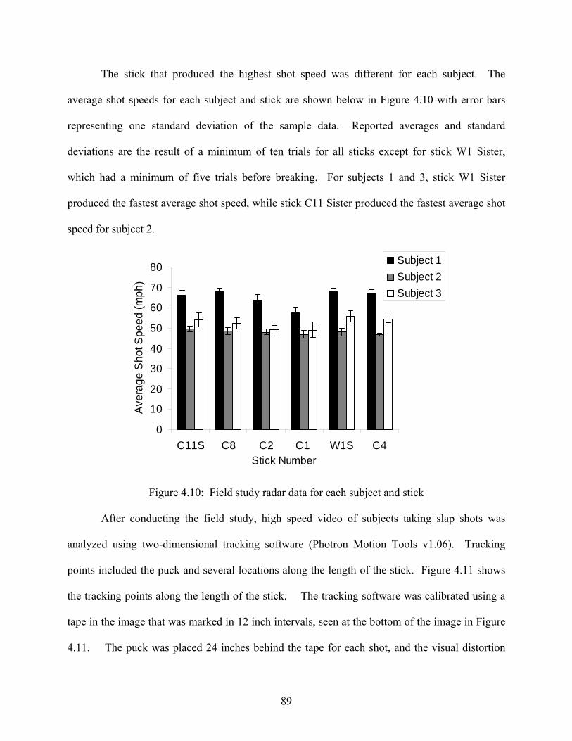
The stick that produced the highest shot speed was different for each subject. The
average shot speeds for each subject and stick are shown below in Figure 4.10 with error bars
representing one standard deviation of the sample data. Reported averages and standard
deviations are the result of a minimum of ten trials for all sticks except for stick W1 Sister,
which had a minimum of five trials before breaking. For subjects 1 and 3, stick W1 Sister
produced the fastest average shot speed, while stick C11 Sister produced the fastest average shot
speed for subject 2.
0
10
20
30
40
50
60
70
80
C11S C8 C2 C1 W1S C4Stick Number
Ave
rage
Sho
t Spe
ed (m
ph)
Subject 1Subject 2Subject 3
Figure 4.10: Field study radar data for each subject and stick
After conducting the field study, high speed video of subjects taking slap shots was
analyzed using two-dimensional tracking software (Photron Motion Tools v1.06). Tracking
points included the puck and several locations along the length of the stick. Figure 4.11 shows
the tracking points along the length of the stick. The tracking software was calibrated using a
tape in the image that was marked in 12 inch intervals, seen at the bottom of the image in Figure
4.11. The puck was placed 24 inches behind the tape for each shot, and the visual distortion
89
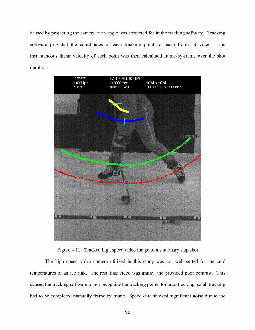
caused by projecting the camera at an angle was corrected for in the tracking software. Tracking
software provided the coordinates of each tracking point for each frame of video. The
instantaneous linear velocity of each point was then calculated frame-by-frame over the shot
duration.
Figure 4.11: Tracked high speed video image of a stationary slap shot
The high speed video camera utilized in this study was not well suited for the cold
temperatures of an ice rink. The resulting video was grainy and provided poor contrast. This
caused the tracking software to not recognize the tracking points for auto-tracking, so all tracking
had to be completed manually frame by frame. Speed data showed significant noise due to the
90
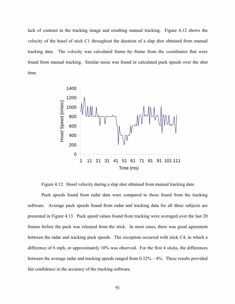
lack of contrast in the tracking image and resulting manual tracking. Figure 4.12 shows the
velocity of the hosel of stick C1 throughout the duration of a slap shot obtained from manual
tracking data. The velocity was calculated frame–by–frame from the coordinates that were
found from manual tracking. Similar noise was found in calculated puck speeds over the shot
time.
0
200
400
600
800
1000
1200
1400
1 11 21 31 41 51 61 71 81 91 101 111Time (ms)
Hos
el S
peed
(in/
sec)
Figure 4.12: Hosel velocity during a slap shot obtained from manual tracking data
Puck speeds found from radar data were compared to those found from the tracking
software. Average puck speeds found from radar and tracking data for all three subjects are
presented in Figure 4.13. Puck speed values found from tracking were averaged over the last 20
frames before the puck was released from the stick. In most cases, there was good agreement
between the radar and tracking puck speeds. The exception occurred with stick C4, in which a
difference of 6 mph, or approximately 10% was observed. For the first 4 sticks, the differences
between the average radar and tracking speeds ranged from 0.32% – 4%. These results provided
fair confidence in the accuracy of the tracking software.
91

0
10
20
30
40
50
60
70
80
C11S C8 C2 C1 C4Stick Number
Ave
rage
Puc
k S
peed
(mph
)
RadarTracking
Figure 4.13: Comparison of average puck speeds found from radar data and tracking software
The first primary goal of the field study was to measure the swing speed of the stick
during a slap shot at the time of stick-puck contact. This measurement was important in
confirming the value chosen for the nominal stick swing speed, vn used to calculate the swing
speed in performance testing, vs discussed previously in Section 2.3, Equation (2.21).
In Figure 4.12 above, three distinct phases of the shot can be observed in the velocity
data. The first 40 ms show the downswing phase of the slap shot, in which the stick is
approaching the ice and the puck. At approximately 40 ms, the shaft and puck loading began,
showing a drastic decrease in the linear velocity of the stick as the shaft was deflected and the
puck began to move. The final phase was the release phase, from roughly 75 ms onward, in
which the stick and puck travel together until the puck was released from the blade toward the
target. These characteristic phases were observed in all of the slap shots with all sticks.
92

In most shots, stick speed during the release phase was slower than the speed during the
downswing phase. This is consistent with the findings of Lomond, et al. [4.2] for recreational
players, in which the downswing phase had an average stick linear velocity of vs = 45.7 mph and
the release phase had an average vs = 33.9 mph. The opposite was found to be true for elite
players, in which the downswing phase had an average vs = 46.4 mph and the release phase had
an average vs = 61.5 mph [4.2].
Tracking data from subject 1 was used to determine the average linear velocity of the
hosel end of the stick during the slap shot in this study. Tracking data from the hosel was
averaged over the time interval after the stick had contacted the puck and before it was released
from the blade. Eight shots from subject 1 were analyzed and an average hosel velocity of 41.0
1.8 mph was found. ±
It was also desirable to compare results to the 20 – 30 rad/sec reported by Sim and Chao
[4.9]. The center of rotation was not reported in their results. In order to directly compare the
results from the current study to those of Sim and Chao, the instantaneous center of rotation of
the stick at the time of puck release needed to be determined. This could be done by determining
the velocity vectors of two points along the length of the stick and determining their point of
intersection. It was determined in this study, however, that too much variation existed in the
velocity vectors to accurately determine a center of rotation. During the short stick – puck
contact time, the shaft deflects and then recoils, causing the lower portion of the stick to rotate
about the kick point, further complicating the determination of the instantaneous center of
rotation.
Overall, stick linear velocity values for subject 1 were found to lie within the range
previously reported in the literature [4.2]. Data obtained from this field study was consistent
93

with recreational player abilities. The performance study considered in the next section was
concerned with high recreational to elite player abilities. Field study findings for the linear
velocity of the stick for a recreational player were in the range of 41 mph. Findings in the
literature report up to 61.5 mph for elite players and 41 mph for recreational players [4.2]. It can
therefore be assumed that an estimate of 60 mph swing speed for an elite player is a reasonable
estimate for this study.
4.4 Performance Testing
There were two main goals in the development of the hockey stick performance test. The
first was to determine if a hockey stick could be tested in a lab setting in a manner similar to
those currently used for testing softball, baseball, and cricket bats [4.4]. The second was to
determine if noticeable differences exist in the lab performance of different types of hockey
sticks.
In this study, a method of testing performance of ice hockey sticks was developed and
implemented to test 17 different sticks. A test fixture was designed to grip the hockey stick and
pivot it freely at the end of a high speed air cannon. The performance test was developed as a
model for a slap shot. A derived value for puck speed after it was shot from the stick was
developed and applied to test data for each hockey stick.
4.4.1 Moment of Inertia
The method for determining the moment of inertia, or I, of hockey sticks was analogous
to the method described in ASTM F2398-04 for softball and baseball bats [4.5]. The stick was
considered as a physical pendulum with the blade acting as a point mass on the end. The stick
was pivoted at a distance of 35 inches from the heel of the blade. The moment of inertia was
94
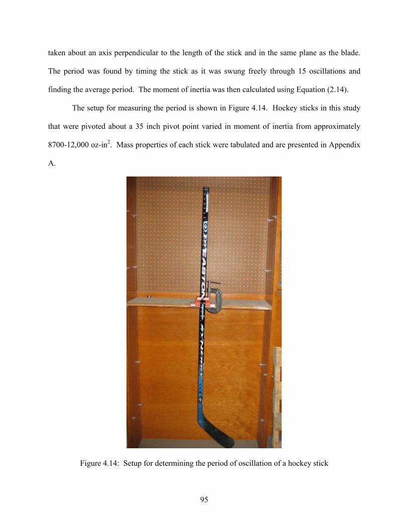
taken about an axis perpendicular to the length of the stick and in the same plane as the blade.
The period was found by timing the stick as it was swung freely through 15 oscillations and
finding the average period. The moment of inertia was then calculated using Equation (2.14).
The setup for measuring the period is shown in Figure 4.14. Hockey sticks in this study
that were pivoted about a 35 inch pivot point varied in moment of inertia from approximately
8700-12,000 oz-in2. Mass properties of each stick were tabulated and are presented in Appendix
A.
Figure 4.14: Setup for determining the period of oscillation of a hockey stick
95

4.4.2 Test Setup
An air cannon similar to the one used for high speed puck testing was used in this study
for testing hockey sticks. The rigid array of load cells was replaced with a pivoted stick. Figure
4.15 shows the test setup. A fixture was designed and fabricated to hold the stick with the blade
positioned at the end of the barrel, shown in Figure 4.16. This fixture allowed the stick to pivot
freely about an axis that was 35 inches from the bottom of the shaft. It was fabricated out of
steel and bolted directly onto the mill base at the end of the cannon.
Figure 4.15: Performance test setup
96
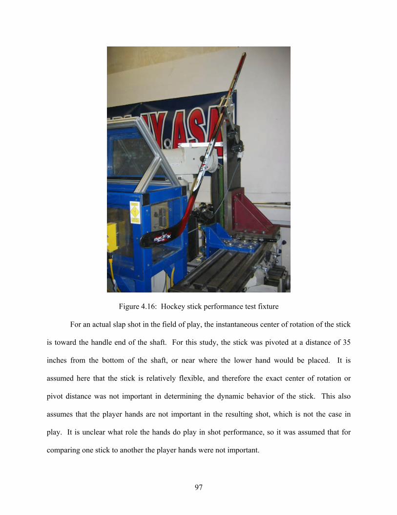
Figure 4.16: Hockey stick performance test fixture
For an actual slap shot in the field of play, the instantaneous center of rotation of the stick
is toward the handle end of the shaft. For this study, the stick was pivoted at a distance of 35
inches from the bottom of the shaft, or near where the lower hand would be placed. It is
assumed here that the stick is relatively flexible, and therefore the exact center of rotation or
pivot distance was not important in determining the dynamic behavior of the stick. This also
assumes that the player hands are not important in the resulting shot, which is not the case in
play. It is unclear what role the hands do play in shot performance, so it was assumed that for
comparing one stick to another the player hands were not important.
97

Pucks were fired at the stick at 50 ± 1 mph and impacted on the lower inch of the blade
of the stick. The speed of 50 mph was chosen in an attempt to ensure that the stick would
withstand an entire scan without breaking. In preliminary testing, sticks that were impacted at
higher speeds showed significant damage before a scan was completed.
Three pairs of ADC iBeam light gates (Automated Design) were used to measure the
inbound speed of the puck. A digital encoder (CUI Inc., Tulatin, OR) attached to the bottom of
the pivot shaft was used to measure the swing speed of the stick after impact. The first 15
degrees of travel of the stick were neglected, and the encoder measured the speed of the stick
over the next 45 degrees. LabView fit a line to the encoder data, reporting the slope as the
average swing speed of the stick.
High speed video and powder spray on the blade of the stick were both used to visually
ensure a good impact. A good impact was defined as one in which the puck passed through all
three light gates within the acceptable speed range, did not wobble or spin, impacted the stick
with the flat edge of the puck, and impacted the stick only once. During the test, stick and puck
velocity were considered positive in the direction that the puck was fired, or to the right in Figure
4.15.
For each stick, a scan across the blade to find the location of maximum performance was
completed. Impact locations started at the heel of the blade and moved horizontally across the
blade in one inch intervals. Eight impact locations were utilized for each stick, covering the area
of the blade where the puck would typically impact in a slap shot during play. Each location was
impacted with six different pucks, and reported performance values were the averages from all
six pucks. Pucks were rotated and impacted every sixth fire in an attempt to regulate puck
98
warming. An infrared temperature sensor was used to ensure that puck temperatures stayed
within 72 2° F during testing. ±
It is important to discuss the concept of shaft loading when considering this test method.
In an actual slap shot, the resulting puck speed is due to a combination of shaft loading and
swing speed of the stick. The small effect of stick stiffness on puck velocity [4.1] suggests that
stick speed and deflection increase with player ability [4.3]. Thus, the amount of energy
available for a player to swing and deflect the shaft can be viewed as constant for a given player,
regardless of the stiffness of the stick.
Energy stored by deflecting the stick to a distance of x can be viewed in terms of a linear
spring, or
2
21 kxU = (4.3)
for a shaft of stiffness k. For the energy to be constant, a stick with a lower stiffness value must
deflect more than a stick with a higher stiffness value. Stiffer sticks have been found to deflect
less during shots than more compliant sticks in previous research [4.1]. Shaft loading may be
viewed as a constant increase in stick speed (independent of shaft stiffness) that may be
accounted for in the stick swing speed.
4.4.3 Data Reduction
The performance measure for puck speed (vp) is a derived value to quantify ideal stick
performance. First, a slap shot with an initially stationary puck and a moving stick was
considered. The frame of reference for the test was then changed to a stationary stick and a
moving puck. Changing the frame of reference aligns the data reduction process with the test
method of firing a puck at a stationary pivoted stick.
99

The puck was fired through three sets of light gates that measured the inbound speed, V1.
The swing speed of the stick, ω2 (rad/s) after impact was then measured using a digital encoder.
After impacting the blade, the puck continued moving in the positive direction, making its
velocity after impact difficult to measure. The derivation of performance calculations is detailed
in Section 2.3, Equations (2.13) – (2.21).
The impact location, Q was the perpendicular distance from the pivot axis to the location
on the blade where the puck impacted, shown in Figure 4.17. Knowing both the horizontal and
vertical distances from the pivot axis to the impact location, the value Q was calculated using the
Pythagorean Theorem.
Pivot Qj
Qi
Figure 4.17: Calculation of impact location
The calculated swing speed is the result of a nominal swing speed, vn, that is scaled for
stick inertia, I and impact location, shown previously in Equation (2.21). Nominal swing speed,
inertia, and impact location values were needed. The nominal impact location chosen was 35
inches, which corresponds to an impact at the heel of the blade. This was selected in order to
keep performance calculations consistent with the measured and observed swing speeds used to
100

determine the nominal stick swing speed, vn. Stick swing speeds calculated in the field study and
from angular velocities found in the literature were calculated at the heel of the blade. The linear
velocity of the stick at the time of impact then increased as the impact location moves across the
blade toward the toe. The inertia of the sticks tested in this study ranged from roughly 8000 –
12,000 oz-in2. A median value of 10,000 oz-in2 was chosen for this study.
Finally, a nominal stick swing speed of vn = 60 mph (1056 in/sec) was chosen, making
Equation (2.21):
4/1000,1035
60 ⎟⎠⎞
⎜⎝⎛⎟⎠⎞
⎜⎝⎛=
IQvs (4.4)
This value was selected based on field study calculations, and previous research that measured
the angular velocity of hockey sticks during slap shots.
The swing speed was used to calculate a puck speed based on a moving stick and a
stationary puck. For this case, Equation (2.20) reduces to
( )asp evv += 1 (4.5)
Once the swing speed was calculated for each impact, vs was substituted into Equation (4.5),
yielding a puck velocity that represents a modeled speed of a puck coming off the stick in a slap
shot. The values for puck speed from six pucks were averaged at each impact location and
plotted along the length of the blade. Impact locations were numbered 1 – 8, with 1
corresponding to an impact at the heel of the blade and each successive number representing a
one inch horizontal interval toward the toe of the blade.
4.4.4 Stick Comparison
Seventeen sticks were performance tested in this study, summarized in Table 4.1. Two
stick variables were investigated for performance: stick material and shaft taper. Wood and
101
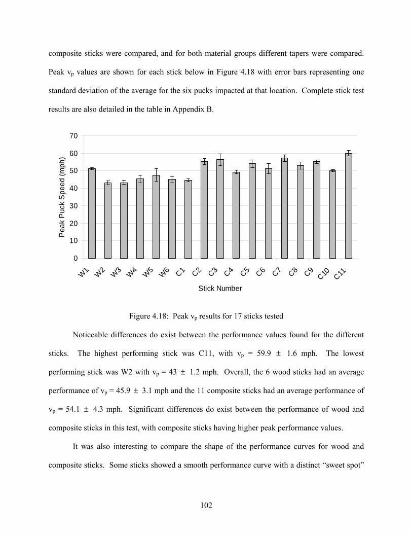
composite sticks were compared, and for both material groups different tapers were compared.
Peak vp values are shown for each stick below in Figure 4.18 with error bars representing one
standard deviation of the average for the six pucks impacted at that location. Complete stick test
results are also detailed in the table in Appendix B.
0
10
20
30
40
50
60
70
W1 W2 W3 W4 W5 W6 C1 C2 C3 C4 C5 C6 C7 C8 C9C10 C11
Stick Number
Pea
k P
uck
Spe
ed (m
ph)
Figure 4.18: Peak vp results for 17 sticks tested
Noticeable differences do exist between the performance values found for the different
sticks. The highest performing stick was C11, with vp = 59.9 ± 1.6 mph. The lowest
performing stick was W2 with vp = 43 ± 1.2 mph. Overall, the 6 wood sticks had an average
performance of vp = 45.9 3.1 mph and the 11 composite sticks had an average performance of
v
±
p = 54.1 4.3 mph. Significant differences do exist between the performance of wood and
composite sticks in this test, with composite sticks having higher peak performance values.
±
It was also interesting to compare the shape of the performance curves for wood and
composite sticks. Some sticks showed a smooth performance curve with a distinct “sweet spot”
102

along the blade. Others exhibited more erratic performance curves, sometimes increasing in
performance until the very end of the blade, in which case a definite peak was not shown.
Performance curves for three sticks are shown below in Figure 4.19 to illustrate this point. Stick
C5 showed a definite sweet spot and performance peak. The other two sticks had erratically
changing performance across the blade and peak performance values occurred either at the heel
or toe end of the blade. Of the wood sticks tested, all except stick W6 exhibited erratic
performance curves with no definite sweet spot. Of the composite sticks tested, all except sticks
C1 and C3 showed smooth performance curves with definite sweet spots.
35
40
45
50
55
0 2 4 6 8 10Impact Location (in from heel)
Puc
k S
peed
(mph
)
C5W2C1
Figure 4.19: Sample performance curves for three sticks
Shaft taper appeared to have a less definite effect on peak performance results. For the
wood sticks, W5 and W6 have tapered shafts, while the rest have straight shafts. For wood,
tapered shafts do not appear to result in a significant increase in peak performance. The
performance of W1 was significantly higher than that of the other wood sticks, but performance
differences between the other 5 wood sticks do not appear to be significant.
103
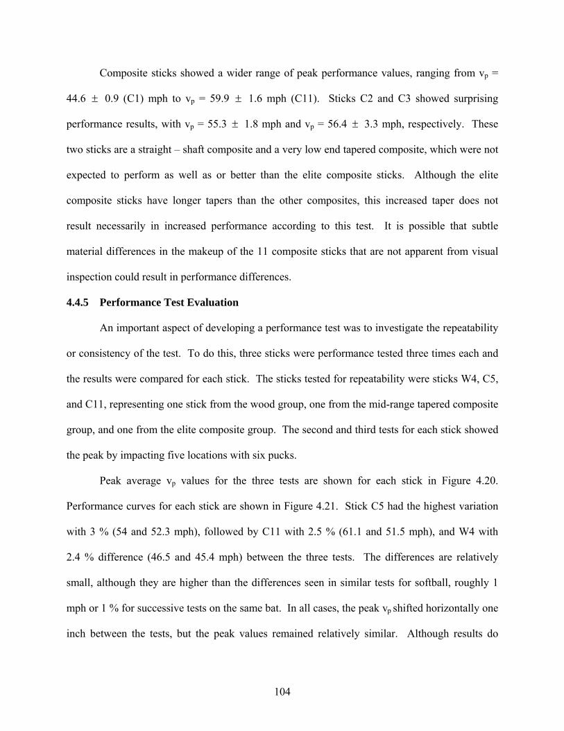
Composite sticks showed a wider range of peak performance values, ranging from vp =
44.6 0.9 (C1) mph to v± p = 59.9 ± 1.6 mph (C11). Sticks C2 and C3 showed surprising
performance results, with vp = 55.3 ± 1.8 mph and vp = 56.4 ± 3.3 mph, respectively. These
two sticks are a straight – shaft composite and a very low end tapered composite, which were not
expected to perform as well as or better than the elite composite sticks. Although the elite
composite sticks have longer tapers than the other composites, this increased taper does not
result necessarily in increased performance according to this test. It is possible that subtle
material differences in the makeup of the 11 composite sticks that are not apparent from visual
inspection could result in performance differences.
4.4.5 Performance Test Evaluation
An important aspect of developing a performance test was to investigate the repeatability
or consistency of the test. To do this, three sticks were performance tested three times each and
the results were compared for each stick. The sticks tested for repeatability were sticks W4, C5,
and C11, representing one stick from the wood group, one from the mid-range tapered composite
group, and one from the elite composite group. The second and third tests for each stick showed
the peak by impacting five locations with six pucks.
Peak average vp values for the three tests are shown for each stick in Figure 4.20.
Performance curves for each stick are shown in Figure 4.21. Stick C5 had the highest variation
with 3 % (54 and 52.3 mph), followed by C11 with 2.5 % (61.1 and 51.5 mph), and W4 with
2.4 % difference (46.5 and 45.4 mph) between the three tests. The differences are relatively
small, although they are higher than the differences seen in similar tests for softball, roughly 1
mph or 1 % for successive tests on the same bat. In all cases, the peak vp shifted horizontally one
inch between the tests, but the peak values remained relatively similar. Although results do
104

show some differences, all results lie within one standard deviation for each stick, indicating that
the differences are not significant.
0
10
20
30
40
50
60
70
1 2 3 4 5 6 7 8 9
Pea
k P
uck
Spe
ed (m
ph)
C11C5W4
Figure 4.20: Repeatability of peak vp for three sticks
37
42
47
52
57
62
67
0 2 4 6Impact Location (in from heel)
Puc
k S
peed
(mph
)
Test 1Test 2Test 3
(a)
105

37
42
47
52
57
62
0 2 4 6Impact Location (in from heel)
Puc
k S
peed
(mph
)
Test 1Test 2Test 3
(b)
37
39
41
43
45
47
49
0 2 4 6Impact Location (in from heel)
Puc
k S
peed
(mph
)
Test 1Test 2Test 3
(c)
Figure 4.21: Repeated performance curves for (a) C11, (b) C5, and (c) W4
Sticks in this study were impacted along the lower inch of the blade during performance
testing. It was desirable to determine the effect, if any, of the vertical impact location on
performance results. A scan was completed on one hockey stick by fixing the horizontal pivot
106
distance at the middle of the blade and impacting the blade in vertical intervals of 0.2 inches.
The stick was impacted with 6 pucks at each location and averages from the 6 impacts are
reported as vp values here. The first impact location corresponds to the bottom edge of the puck
impacting the bottom of the blade. Results are presented below in Figure 4.22.
34
36
38
40
42
44
46
0 0.2 0.4 0.6 0.8 1 1.2 1.4 1.6 1.8Vertical Blade Position (in)
Puc
k S
peed
(mph
)
Figure 4.22: Vertical blade position test results
Performance values remained essentially constant along the lower half of the blade, and
then showed larger changes. At the 1.2 inch impact location, vp results were 10.7% higher (vp =
41.2 3.8 mph) than at the first location at the bottom of the blade (v± p = 36.9 1.1 mph). As
the impact location moved toward the top of the blade, more scatter was seen in the results, as is
evident by the increasingly large error bars in Figure 4.22. It is postulated that impacting the
blade toward the top caused increased vibration in the shaft and blade of the stick, therefore
resulting in less consistent data at those locations. Stick vibration during performance testing is
discussed further below.
±
107

Further testing examined the effect of puck temperature on performance test results. One
stick (C1) was tested first with six pucks that were at room temperature, or 72 2° F. It was
then tested again at six locations with three frozen pucks at 25
±
± 2° F. A non-contact infrared
temperature sensor was used to verify puck temperature before firing. Performance curves for
both tests are shown in Figure 4.23. No significant difference in performance was observed
when different temperature pucks were used. Although puck temperature has significant effects
on the elasticity and controllability of a puck, these results implied that puck temperature is not
important in determining the dynamic behavior of a hockey stick. This also implies that the
stiffness of the puck is not important in determining the dynamic behavior of the stick.
30
32
34
36
38
40
42
44
46
48
0 1 2 3 4 5 6 7 8Distance from heel
Puc
k sp
eed
(mph
)
room temp puckscold pucks
Figure 4.23: Performance results for a stick tested with warm and frozen pucks
It is highly desirable in sports equipment testing to show a correlation between lab
performance and performance in the field of play. Radar data from subject 1 in the field study
was compared to the cannon performance test data in an attempt to find a correlation. Results
are compared in Figure 4.24. In both cases, stick C1 had the slowest puck speed. The small
sample size of the field study prevented any other correlations between lab and on-ice
108
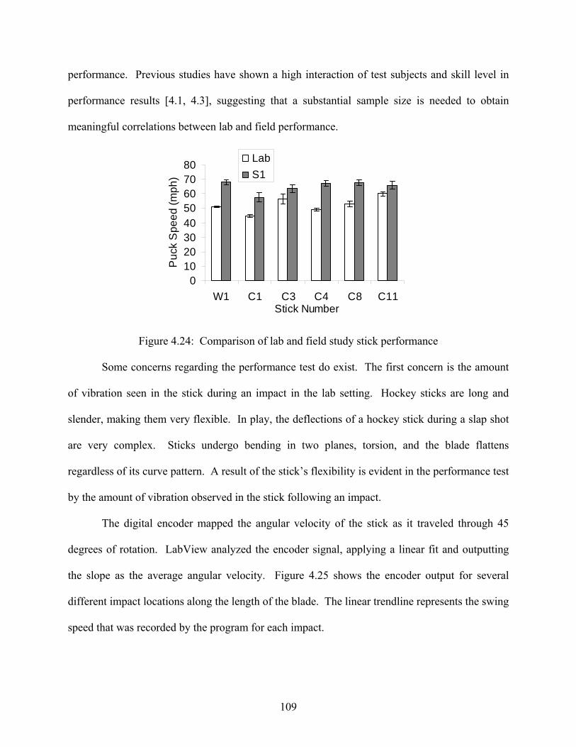
performance. Previous studies have shown a high interaction of test subjects and skill level in
performance results [4.1, 4.3], suggesting that a substantial sample size is needed to obtain
meaningful correlations between lab and field performance.
01020304050607080
W1 C1 C3 C4 C8 C11Stick Number
Puc
k S
peed
(mph
)LabS1
Figure 4.24: Comparison of lab and field study stick performance
Some concerns regarding the performance test do exist. The first concern is the amount
of vibration seen in the stick during an impact in the lab setting. Hockey sticks are long and
slender, making them very flexible. In play, the deflections of a hockey stick during a slap shot
are very complex. Sticks undergo bending in two planes, torsion, and the blade flattens
regardless of its curve pattern. A result of the stick’s flexibility is evident in the performance test
by the amount of vibration observed in the stick following an impact.
The digital encoder mapped the angular velocity of the stick as it traveled through 45
degrees of rotation. LabView analyzed the encoder signal, applying a linear fit and outputting
the slope as the average angular velocity. Figure 4.25 shows the encoder output for several
different impact locations along the length of the blade. The linear trendline represents the swing
speed that was recorded by the program for each impact.
109
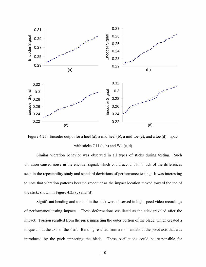
0.23
0.25
0.27
0.29
0.31
(a)
Enc
oder
Sig
nal
0.22
0.23
0.24
0.25
0.26
0.27
(b)
Enc
oder
Sig
nal
0.22
0.24
0.26
0.28
0.3
0.32
(c)
Enc
oder
Sig
nal
0.22
0.24
0.26
0.28
0.3
0.32
(d)
Enc
oder
Sig
nal
Figure 4.25: Encoder output for a heel (a), a mid-heel (b), a mid-toe (c), and a toe (d) impact
with sticks C11 (a, b) and W4 (c, d)
Similar vibration behavior was observed in all types of sticks during testing. Such
vibration caused noise in the encoder signal, which could account for much of the differences
seen in the repeatability study and standard deviations of performance testing. It was interesting
to note that vibration patterns became smoother as the impact location moved toward the toe of
the stick, shown in Figure 4.25 (c) and (d).
Significant bending and torsion in the stick were observed in high speed video recordings
of performance testing impacts. These deformations oscillated as the stick traveled after the
impact. Torsion resulted from the puck impacting the outer portion of the blade, which created a
torque about the axis of the shaft. Bending resulted from a moment about the pivot axis that was
introduced by the puck impacting the blade. These oscillations could be responsible for
110

introducing unpredictable variations in measured swing speed data, causing higher standard
deviations in test data.
In elite-level play, puck speeds resulting from slap shots often reach speeds of 80 – 100
mph [4.1, 4.2, 4.11]. In the field study conducted for this research, top puck speeds were
approximately 70 mph. The performance test utilized a faster stick swing speed than that found
in the field study, but puck speeds were found to be much slower, in the range of 44.4 – 59.9
mph. It is suspected that this discrepancy can be explained in terms of stick – puck contact time
and shaft loading.
It is suspected that the stick and puck exhibit an extended trampoline effect in an actual
slap shot, in which the flex stored in the shaft is releasing at approximately the same time the
puck leaves the stick. Previous research has found the stick-puck contact time for slap shots to
be in the range of 38 9 ms for elite players and 27 ± ± 5 ms for recreational players [4.3]. Field
study data from recreational players in this study found contact times for recreational players in
the range of 32 5 ms. In the cannon impact testing, the stick-puck contact time was found
between 5 – 10 ms. It is postulated here that the shorter contact duration in the lab testing
prevents the full effects of shaft loading on the final puck speed than actually occurs on ice,
where contact times are roughly four times longer. The shorter contact time in lab testing does
not allow sufficient transfer of bending energy from the shaft to the puck during the impact.
±
This theory can be examined in more detail by considering puck speed as a result of both
inertia and potential energy stored in the shaft of the stick. First, let us consider a stick with a lab
performance rating of vp = 50 mph, which is roughly the median of sticks tested in this study.
For the moment, it is assumed that shaft loading produces no effect on lab performance. Assume
that during an actual slap shot, the puck has reached this speed at the time of maximum shaft
111

deflection during the shot. The kinetic energy of the puck after it leaves the stick must be
equivalent to the total energy of the moving stick/puck and the potential energy of the deflected
shaft at its peak deflection. Or mathematically,
222
21
21
21
fppp vmkxvm =+ (4.6)
where mp is the mass of the puck, vp is the puck speed found from lab performance testing, k is
the stiffness of the stick (lb/in), x is the displacement of the shaft (in), and vf is the final puck
speed due to both inertial and potential energy effects. This equation can be solved for the final
puck speed, vf, yielding:
2/122
⎥⎥⎦
⎤
⎢⎢⎣
⎡ +=
p
ppf m
kxvmv (4.7)
Three point bend tests were performed on the 17 sticks tested in this study. A 50 inch
span was used to deflect the stick in a load frame (MTS Systems Corporation, Eden Prairie,
MN), and maximum force values were recorded every 0.2 inches to develop a force –
displacement curve. The test setup for measuring bending stiffness is shown in Figure 4.26. In
this case, the stiffness of the shaft was considered, while the stiffness of the blade was neglected.
Figure 4.27 shows some of the force – displacement curves that were found. All sticks showed a
linear force – displacement profile and stiffness values were found to range from 34.2 – 49.0
lb/in. Stiffness values for each stick are given in Appendix B, Table B.3. This value represented
the 3-point bending stiffness of the sticks, or k in Equation (4.7).
112

Figure 4.26: Stick bending stiffness test setup
05
101520253035404550
0 0.2 0.4 0.6 0.8 1Deflection (in)
Load
(lbs
)
C7W3C2
Figure 4.27: Stick stiffness results from 3-point bend tests
By taking mp to be an average puck mass of 5.8 oz, Equation (4.7) was plotted as a
function of shaft displacement, x in Figure 4.28 for a range of shaft stiffness from k = 0 (no shaft
loading) to k = 40 lb/in. To achieve a final puck speed of 70 mph with the 40 lb/in stick, a shaft
113

deflection of approximately 4 inches is required. With a shaft deflection of 6 inches, a final puck
speed of approximately 85 mph can be obtained. These deflections are within the range
commonly seen in high level player slap shot, in which bending in the shaft can be as much as 16
- 30° [4.1, 4.12].
40
50
60
70
80
90
100
110
0 1 2 3 4 5 6 7Shaft Deflection (in)
Puc
k S
peed
(mph
)
k=0k=30k=40k=50
Figure 4.28: Final puck speed as a function of shaft deflection
It is believed that shaft loading does play some role in the lab performance results
because no correlation between the inertia of the stick and stick performance was noted in this
study. Still, the preceding argument provides a plausible explanation for the slower puck speeds
seen in lab performance compared to on-ice performance. For a stick that is more compliant
than the one described here, the decreased stiffness would result in an increased deflection for
the same final puck speed.
Measured stick stiffness was also used to evaluate the validity of the assumption that
stick stiffness can be neglected for the lab test. For each stick tested, a shaft loading factor was
114
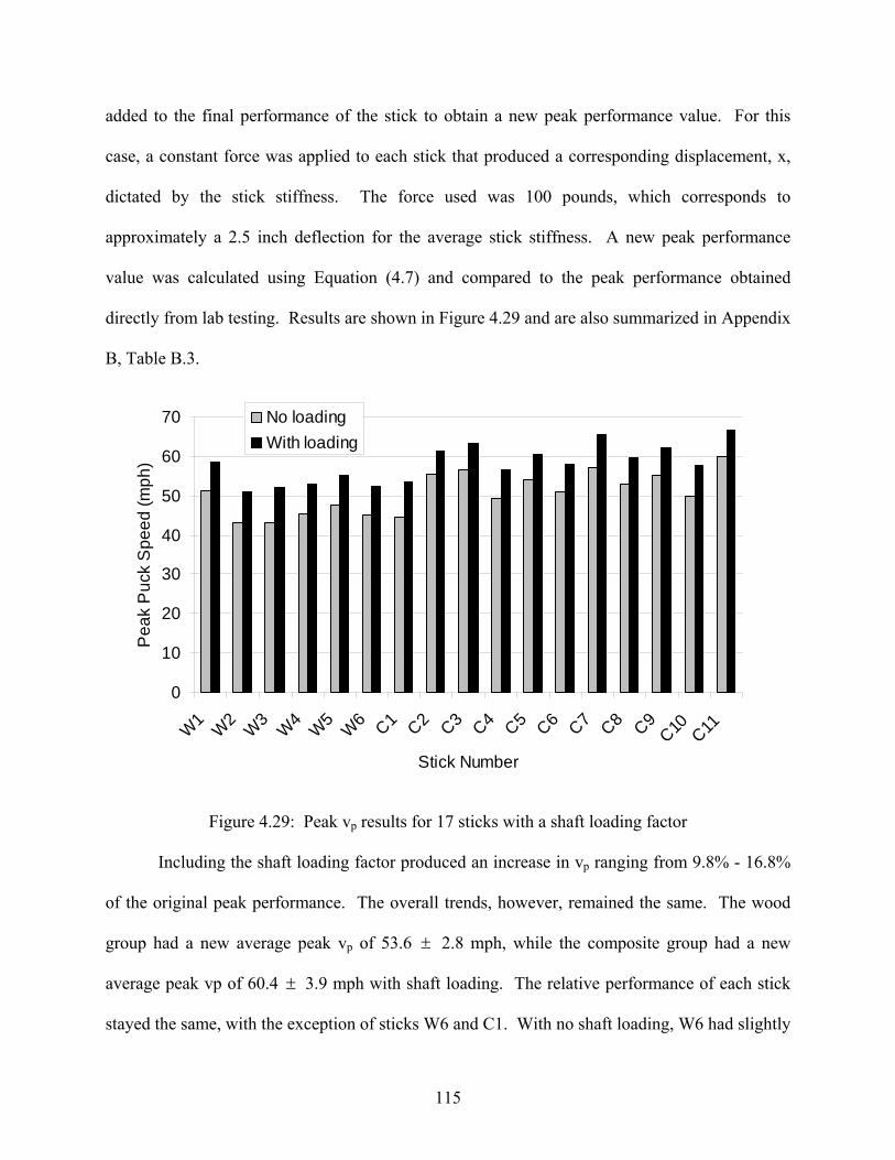
added to the final performance of the stick to obtain a new peak performance value. For this
case, a constant force was applied to each stick that produced a corresponding displacement, x,
dictated by the stick stiffness. The force used was 100 pounds, which corresponds to
approximately a 2.5 inch deflection for the average stick stiffness. A new peak performance
value was calculated using Equation (4.7) and compared to the peak performance obtained
directly from lab testing. Results are shown in Figure 4.29 and are also summarized in Appendix
B, Table B.3.
0
10
20
30
40
50
60
70
W1 W2 W3 W4 W5 W6 C1 C2 C3 C4 C5 C6 C7 C8 C9C10 C11
Stick Number
Pea
k P
uck
Spe
ed (m
ph)
No loadingWith loading
Figure 4.29: Peak vp results for 17 sticks with a shaft loading factor
Including the shaft loading factor produced an increase in vp ranging from 9.8% - 16.8%
of the original peak performance. The overall trends, however, remained the same. The wood
group had a new average peak vp of 53.6 ± 2.8 mph, while the composite group had a new
average peak vp of 60.4 3.9 mph with shaft loading. The relative performance of each stick
stayed the same, with the exception of sticks W6 and C1. With no shaft loading, W6 had slightly
±
115
higher performance than C1, while the opposite was true with shaft loading. These findings
show that a shaft loading factor produces an increase in lab performance, but does not change the
relative performance of one stick to another. The assumption of neglecting stick stiffness in the
performance test can therefore be considered valid.
Several sticks broke during the performance test. It is significant here to note the mode
of failure in these cases. In all cases, sticks failed in a manner that is consistent with failure seen
in the field of play. The major methods of failure were: shaft breaking at the hosel or blade-
shaft junction, shaft breaking in the middle, shaft delamination, and blade delamination. Some
failed sticks are shown below in Figure 4.30.
All of these failure modes were identified by Hoerner [4.11] as common failures that
occur during play. In order of most frequent to least frequent, he found: hosel broke (44 %), the
shaft broke (16 %), shaft delaminated (15 %), and blade delamination (11 %). Hoerner also
identified fracture of the blade as another failure mechanism (15 % frequency), but this type of
failure was not observed in the current study.
116
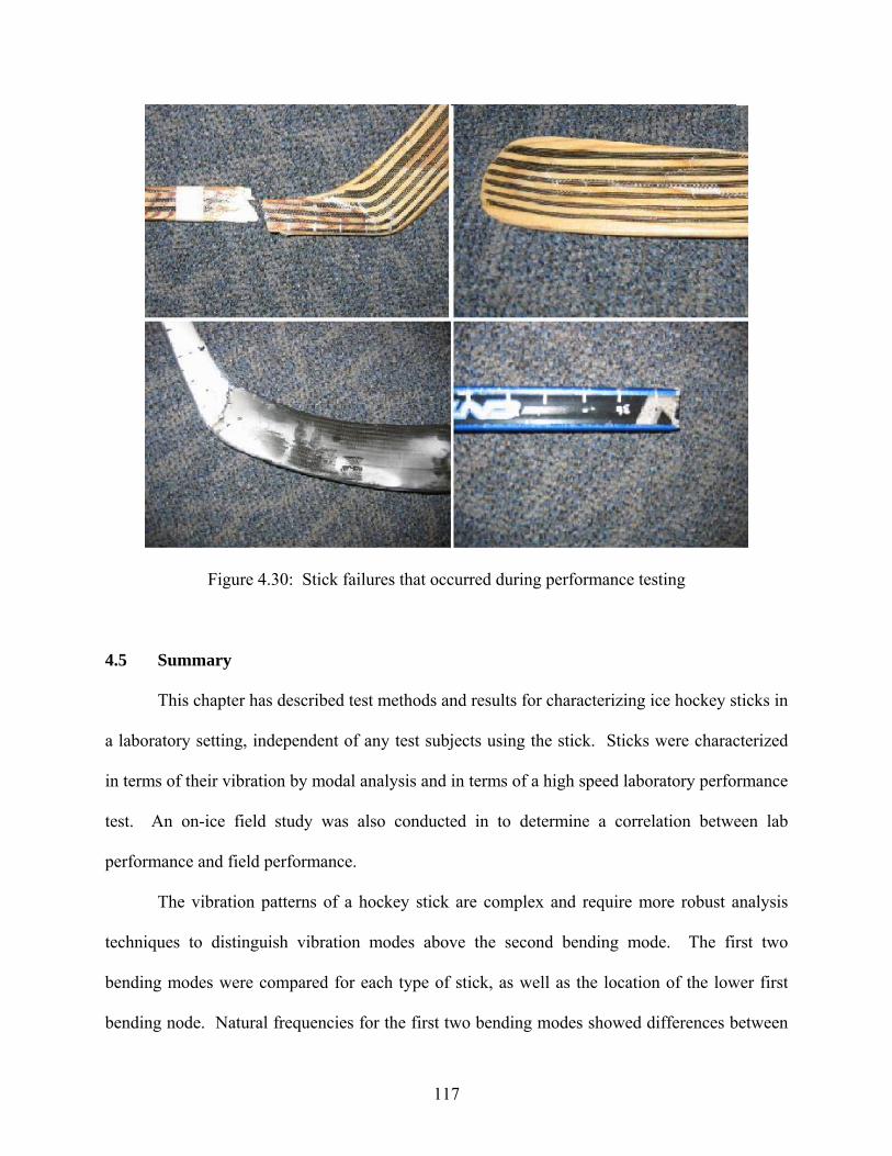
Figure 4.30: Stick failures that occurred during performance testing
4.5 Summary
This chapter has described test methods and results for characterizing ice hockey sticks in
a laboratory setting, independent of any test subjects using the stick. Sticks were characterized
in terms of their vibration by modal analysis and in terms of a high speed laboratory performance
test. An on-ice field study was also conducted in to determine a correlation between lab
performance and field performance.
The vibration patterns of a hockey stick are complex and require more robust analysis
techniques to distinguish vibration modes above the second bending mode. The first two
bending modes were compared for each type of stick, as well as the location of the lower first
bending node. Natural frequencies for the first two bending modes showed differences between
117

the sticks. The wood sticks had lower frequencies than the composite sticks, though differences
were very small. It is suspected that higher frequencies are responsible for characterizing player
perceived feel of a stick. Composite sticks exhibited lower node locations than wood sticks,
indicating a lower kick point in composite sticks.
A high speed laboratory performance test was developed to compare 17 sticks. Notable
differences were found in the performance results of wood and composite sticks. Composite
sticks performed better than wood sticks with an average peak performance of vp = 54.1 ± 4.3
mph, compared to vp = 45.9 3.1 mph for the wood group. The test was shown to have
repeatability within 2.4 – 3 % for three sticks that were tested three times each. Sticks were
impacted along the lower inch of the blade in this study to emulate stick-puck contact seen in
play. The vertical impact location on the blade was shown to have a small effect (9%) on the
performance of the stick, but impacting the blade at higher locations increased the variation of
the results. Puck temperature and dynamic stiffness was shown here to be unimportant in
determining the dynamic behavior of hockey sticks.
±
118
REFERENCES [4.1] Pearsall, D.J., Montgomery, D.L., Rothsching, N., and Turcotte, R.A. The Influence of
Stick Stiffness on the Performance of Ice Hockey Slap Shots. Sports Engineering 2, p.3-11 (1999).
[4.2] V. Lomond, R.A. Turcotte, and D.J. Pearsall, Three-dimensional analysis of blade
contact in an ice hockey slap shot, in relation to player skill. Sports Engineering 7, p. 87-100 (2007).
[4.3] A. Villaseñor, A., Turcotte, R.A. and Pearsall, D.J. Recoil Effect of the Hockey Stick
During a Slap Shot. Journal of Applied Biomechanics, Vol. 22, p. 202-211 (2006). [4.4] ASTM F 2219-04, Standard Test Method for Measuring High Speed Bat Performance
Factor, ASTM International 2004. [4.5] ASTM F 2398-04, Standard Test Method for Measuring Moment of Inertia and Center of
Percussion of a Baseball or Softball Bat, ASTM International 2004. [4.6] Nathan, A.M., Characterizing the performance of baseball bats, Am. J. Phys. 71(2), p.
134-143, 2003. [4.7] Cross, R. and Bower, R., Effects of swing-weight on swing speed and racket power, J.
Sports Sciences 24(1), p. 23-30, 2006. [4.8] Bahill, T. The Ideal Moment of Inertia for a Baseball or Softball Bat, IEEE Transactions
on Systems, Man, and Cybernetics – Part A: Systems and Humans 34(2), p. 197-204, 2004.
[4.9] Sim, F.H. and Chao, E.Y., Injury Potential in Modern Ice Hockey, American Journal of
Sports Medicine, Vol. 6, pp. 378-384, 1978. [4.10] Hoerner, E.F., The Dynamic Role Played by the Ice Hockey Stick, Safety in Ice Hockey,
ASTM STP 1050 1, p. 154-163 (1989). [4.11] Hache, Alain, The Physics of Ice Hockey, The Johns Hopkins University Press, Baltimore
and London (2002). ISBN: 0-8018-7071-2. [4.12] D.A. Moreno, J.T. Wood, and B.E. Thompson, Dynamic analysis techniques for the
design of the ice hockey stick. The Engineering of Sport 5 (1) (2004). [4.13] McConnell, K.G., Vibration Testing: Theory and Practice, Wiley, New York, 1995.
ISBN: 0-471-30435-2
119

[4.14] Avitabile, P., 101 Ways to Extract Modal Parameters – Which is the one for me?, Proceedings of the International Modal Analysis Conference XXIII, Orlando (2008).
[4.15] A Hocknell, R. Jones, and S. Rothberg, Engineering ‘feel’ in the design of golf club
shafts, The Engineering of Sport, Haake (ed.), Balkema, Rotterdam. ISBN: 90 5410 882 3.
120
CHAPTER FIVE
SUMMARY AND FUTURE WORK
5.1 Summary
5.1.1 Hockey Pucks
Hockey pucks were characterized by their impact properties of coefficient of restitution
(e) and dynamic stiffness (kd). A high speed air cannon was used to fire pucks from two brands
at a rigidly mounted array of load cells. Pucks were tested at speeds ranging from 55 – 85 mph
and at temperatures ranging from 25 - 72° F.
A two-brand comparison at room temperature showed small differences in e, but rather
large differences in kd, 33%. The brand of puck with a higher kd also reached a peak force that
was 20% higher than the other. Both brands were also tested at 25° F and showed 26% and 32%
decreases in e and 488% and 626% increases in kd. Differences in e between the two brands that
were found at room temperatures diminished at lower temperatures. Testing at several
intermediate temperatures showed nonlinear changes in both e and kd. The coefficient of
restitution also decreased fairly linearly with increasing speed. The dynamic stiffness increased
with speed, suggesting that pucks have a relatively high degree of nonlinearity.
5.1.2 Hockey Sticks
Seventeen different stick models were used in this study, comprised of 6 wood and 11
composite. A one-dimensional bending analysis was performed on all sticks to compare natural
frequencies and the location of the lower first bending node. The vibration of hockey sticks is
complex, with torsional modes appearing as mirrors of bending modes above the second bending
mode. Small differences were noted in the first two bending mode frequencies for each stick.
121

Overall, wood sticks had the lowest natural frequencies for modes 1 and 2 and the highest node
locations.
A fixture was designed and fabricated to pivot a hockey stick at the end of a high speed
air cannon. Pucks were fired at a stationary pivoted stick, and momentum principles were used
to calculate a performance measure of puck speed as if it were shot from the stick, or vp. Results
showed significant differences for the different types of sticks. Overall, the composite sticks
performed better than the wood sticks, with an average performance of vp = 54.1 4.3 mph for
composite and v
±
p = 45.9 ± 3.1 mph for wood. Shaft taper was shown to be less important than
stick material in determining the stick performance. Three sticks were tested three times each
and showed variations in peak performance of 2.4 – 3%. While puck temperature was
previously shown to be important for determining the dynamic behavior of the puck, it was not
important in determining the dynamic behavior of the stick in this performance test.
Significant vibrations in the stick during a stick – puck impact were noted, which could
cause noise in the results, reducing the repeatability of the test. In addition, laboratory
performance was notably lower than speeds found on the ice. This was explained in terms of
contact time and a shaft loading factor that increased performance. An on-ice field study was
conducted that utilized three recreational level test subjects and 6 sticks. Stick and puck speeds
obtained in the field study correlated to those seen in play.
5.2 Future Work
5.2.1 Hockey Pucks
This study has provided a firm foundation for the characterization of ice hockey pucks at
speeds closer to those seen in game play. Pucks were compared for different brands, speeds, and
122

temperatures, and each was shown to have differences in impact properties. Further work on this
topic could include determining the combined effect of changing speed and temperature on puck
properties. In addition, it is known that higher stiffness and lower coefficient of restitution are
desirable for players handling the puck. It is unclear, however, what impact these properties
have on other tasks like passing and shooting.
The differences found in impact properties could be useful for both equipment
manufacturers and injury analysis. Understanding the impact properties of pucks at game speeds
is important in determining how to best design protective equipment for players. Implications
could also be made regarding injury mechanisms and likelihood for pucks traveling at different
speeds or temperatures.
5.2.2 Hockey Sticks
A suggestion for future work would include examining higher frequency vibration
patterns of hockey sticks. More robust analysis techniques would be needed to do so in order to
examine bending in two dimensions. It is suspected that it may be possible to synchronize
different vibration patterns of the stick in order to maximize energy transfer to the puck.
Bending in the blade, torsion of the shaft, and bending in the shaft all affect the power of a shot.
It is unclear what frequencies of vibration produce desirable affects on shot speed. In addition,
further damping studies should be investigated to better characterize the vibration of sticks.
A larger scale field study is needed that utilizes players of high skill level to effectively
correlate laboratory and on-ice performance of hockey sticks. Instrumenting hockey sticks to
determine in situ vibration patterns during a field study could also provide useful information
that may be correlated with player perception of feel. Additionally, the movement and
deformation of a hockey stick in a shot is very complex. Three-dimensional tracking software
123

124
would be much better suited to analyze high speed video files than the 2-dimensional software
used in the present study.
A high speed laboratory test that showed statistical differences and repeatable results for
different hockey sticks was developed and implemented in this study. Because this research did
not receive outside funding, test samples were limited mainly to donations from manufacturers.
Sticks tested were all sticks that are manufactured for player use, and not specifically tailored to
meet the needs of this study. This likely led to some interaction affects between different stick
tapers and different composite composition for the composite group. It would be beneficial to
obtain test samples that are specifically tailored to vary only one factor at a time to better see the
results of one stick factor compared to another.
For the performance test, it is assumed that the stick is relatively flexible and that the
hands play little role in the execution of a slap shot. In reality, it has been shown that sticks to
not behave as a free – free system and that the hands are important. While it is clear that the
hands are important in shooting tasks, it is unclear if they are needed to compare the lab
performance of one stick to another. This factor should be investigated in more detail, with
numerical modeling to determine what impact the hands may have on the performance and
execution of slap shots.
Finally, much more could be learned about laboratory vs. on-ice performance by
conducting numerical modeling of both slap shots and on-ice performance. Numerical modeling
could also be used to compare the behavior of a hockey stick in the laboratory performance test
to an actual slap shot in greater detail. The topics previously discussed could also be
investigated through numerical models.
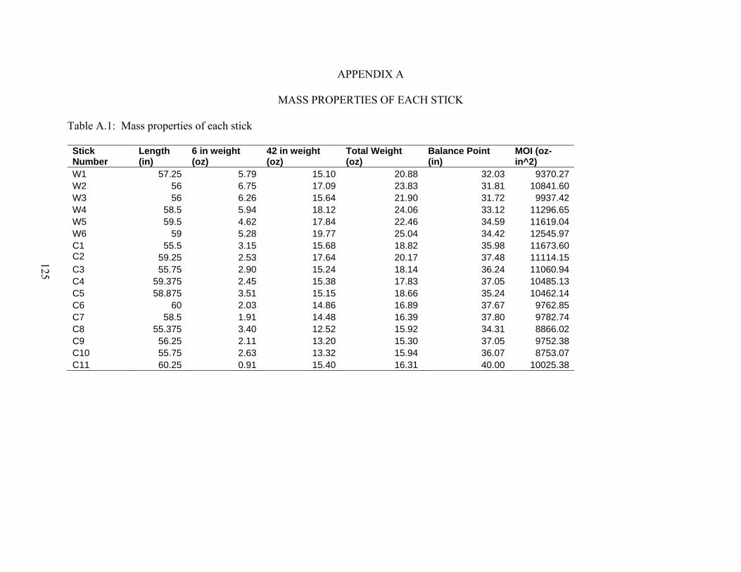
APPENDIX A
MASS PROPERTIES OF EACH STICK
Table A.1: Mass properties of each stick
Stick Number
Length (in)
6 in weight (oz)
42 in weight (oz)
Total Weight (oz)
Balance Point (in)
MOI (oz-in^2)
W1 57.25 5.79 15.10 20.88 32.03 9370.27W2
56 6.75 17.09 23.83 31.81 10841.60W3 56 6.26 15.64 21.90 31.72 9937.42W4 58.5 5.94 18.12 24.06 33.12 11296.65W5 59.5 4.62 17.84 22.46 34.59 11619.04W6 59 5.28 19.77 25.04 34.42 12545.97C1 55.5 3.15 15.68 18.82 35.98 11673.60C2 59.25 2.53 17.64 20.17 37.48 11114.15C3 55.75 2.90 15.24 18.14 36.24 11060.94C4 59.375 2.45 15.38 17.83 37.05 10485.13C5 58.875 3.51 15.15 18.66 35.24 10462.14C6 60 2.03 14.86 16.89 37.67 9762.85C7 58.5 1.91 14.48 16.39 37.80 9782.74C8 55.375 3.40 12.52 15.92 34.31 8866.02C9 56.25 2.11 13.20 15.30 37.05 9752.38C10 55.75 2.63 13.32 15.94 36.07 8753.07C11 60.25 0.91 15.40 16.31 40.00 10025.38
125

APPENDIX B
COMPLETE STICK TESTING RESULTS
Table B.1: Modal analysis results for each stick
Stick Number Material Shaft Geometry MOI (oz- in2 )
Mode 1 Node (in)
Mode 1 Frequency (Hz)
Mode 2 Frequency (Hz)
Damping Ratio
W1 Wood Straight shaft 9370.27 11 48 123 W2
Wood Straight shaft 10841.60 11 51 123 0.00291348W3 Wood Straight shaft 9937.42 10 50 126 0.00282303W4 Wood with composite blade
Straight shaft 11296.65 13 48 120 0.00429556
W5 Wood Tapered shaft 11619.04 11 47 120 0.00398702W6 Wood with composite blade
Tapered shaft 12545.97 11 46 111 0.00466692
C1 Composite Straight shaft 11673.60 8 53 130C2 Composite Straight shaft 11114.15 10 54 137C3 Composite Tapered shaft - low 10444.96 10 51 136 C4 Composite Tapered shaft - mid 10485.13 9 52 136 C5 Composite Tapered shaft - mid 10462.14 10 50 153
C6 CompositeTapered shaft - mid/high 9762.85 10 51 133 0.00175093
C7 Composite Tapered shaft - high
9782.74 9 51 139 0.00230624 C8 Composite Elite composite 9491.08 10 51 137
C9 Composite Elite composite 9752.38 9 59 160C10 Composite Elite composite 8753.07 9 60 161C11 Composite Elite composite 10025.38 9 51 129 0.00202254
126
126
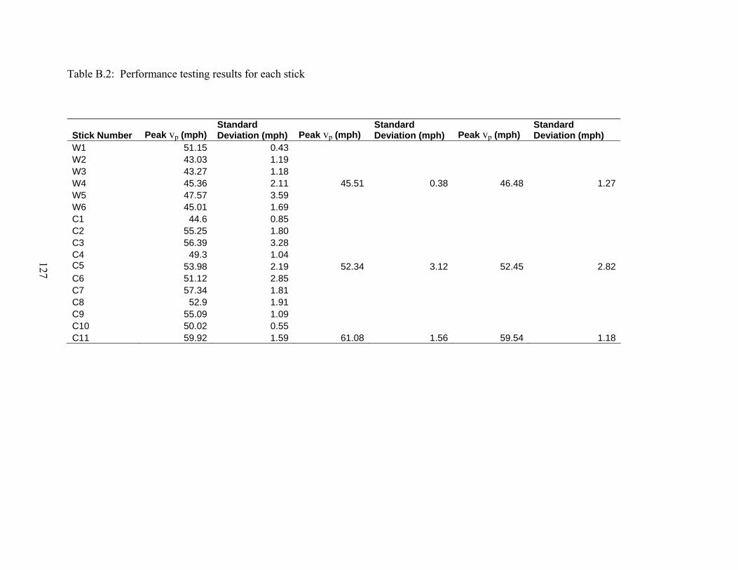
Table B.2: Performance testing results for each stick
Stick Number Peak vp (mph) Standard Deviation (mph) Peak vp (mph)
Standard Deviation (mph) Peak vp (mph)
Standard Deviation (mph)
W1 51.15 0.43 W2
43.03 1.19W3 43.27 1.18W4 45.36 2.11 45.51 0.38 46.48 1.27W5 47.57 3.59W6 45.01 1.69C1 44.6 0.85C2 55.25 1.80C3 56.39 3.28C4 49.3 1.04C5 53.98 2.19 52.34 3.12 52.45 2.82C6 51.12 2.85C7 57.34 1.81C8 52.9 1.91C9 55.09 1.09C10 50.02 0.55C11 59.92 1.59 61.08 1.56 59.54 1.18
127
127
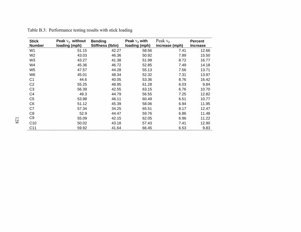
Table B.3: Performance testing results with stick loading
Stick Number
Peak vp without loading (mph)
Bending Stiffness (lb/in)
Peak vp with loading (mph)
Peak vp increase (mph)
Percent Increase
W1 51.15 42.27 58.56 7.41 12.66W2
43.03 46.36 50.92 7.89 15.50W3 43.27 41.38 51.99 8.72 16.77W4 45.36 46.72 52.85 7.49 14.18W5 47.57 44.28 55.13 7.56 13.71W6 45.01 48.34 52.32 7.31 13.97C1 44.6 40.05 53.36 8.76 16.42C2 55.25 48.95 61.28 6.03 9.84C3 56.39 42.55 63.15 6.76 10.70C4 49.3 44.79 56.55 7.25 12.82C5 53.98 46.11 60.49 6.51 10.77C6 51.12 45.39 58.06 6.94 11.95C7 57.34 34.25 65.51 8.17 12.47C8 52.9 44.47 59.76 6.86 11.48C9 55.09 42.15 62.05 6.96 11.22C10 50.02 43.18 57.43 7.41 12.90C11 59.92 41.64 66.45 6.53 9.83
128
128