Experimental Design and Efficiency in fMRIExperimental Design and Efficiency in fMRI

Heidi Bonnici and Sinéad Mullally

Methods for Dummies

13th January 2010

Overview

• Experimental Design– Types of Experimental Design– Timing parameters – Blocked and Event-Related Design

• Design Efficiency– Response vs Baseline (signal-processing)– Response 1 - Response 2 (statistics)

Overview

• Experimental Design– Types of Experimental Design– Timing parameters – Blocked and Event-Related Design

• Design Efficiency– Response vs Baseline (signal-processing)– Response 1 - Response 2 (statistics)

Main Take Home Point of Experimental Design

Make sure you’ve chosen your analysis method and contrasts before you start your experiment

Why is it so important to correctly design your experiment?

• Main design goal: To test specific hypotheses

• We want to manipulate the subject’s experience and behaviour in some way that is likely to produce a functionally specific neurovascular response.

• What can we manipulate?– Stimulus type and properties– Stimulus timing– Subject instructions

Overview

• Experimental Design– Types of Experimental Design– Timing parameters – Blocked and Event-Related Design

• Design Efficiency– Response vs Baseline (signal-processing)– Response 1 - Response 2 (statistics)

Types of Experimental Design

• Categorical – comparing the activity from one task to another task

• Factorial - combining two or more factors within a task and looking at the effect of one factor on the response to other factor

• Parametric – exploring systematic changes in the brain responses according to some performance attributes of task

Categorical Design: Subtraction

Comparing the activity of one task to another task considering the fact that the neural structures supporting cognitive and

behavioural processes combine in a simple additive manner

Can only test for one effect

Example:Task: decide for each noun whether it refers to an animate or inanimate object.

goat bucket

Assumption of pure insertion: One task does not affect the effect of another task.

Categorical Design: Conjunction

Tests multiple effects

Does not depend on pure insertion – conjunction discounts interaction

terms

two or more distinct task pairs each share a common processing difference

common areas of activation for each task pair

Task pairs independent

A-B

(AI-BI) & (AII-BII)

Factorial design

• A – Low attentional load, motion• B – Low attentional load, no motion• C – High attentional load, motion• D – High attentional load, no motion

A B

C D

LOW

LOAD

HIGH

MOTION NO MOTIONLoad task Rees, Frith &

Lavie (1997)

Combining two or more factors within a task and looking at the effect of one factor upon the other/s.

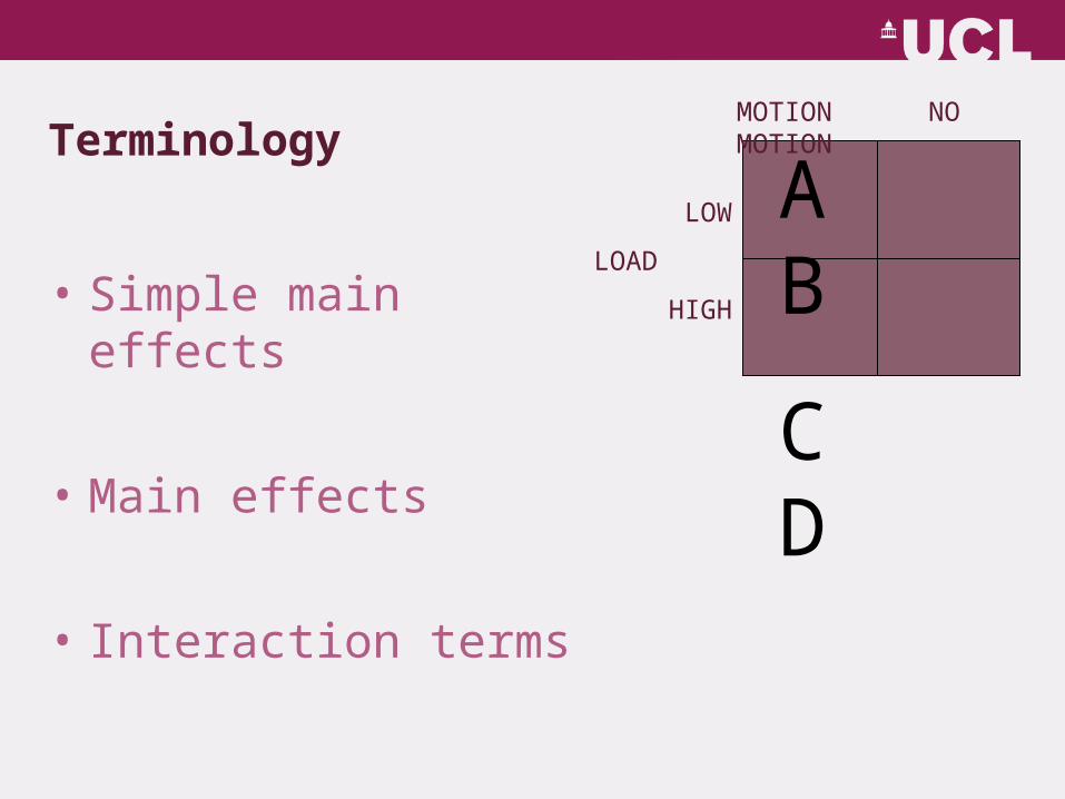
Terminology

• Simple main effects

• Main effects

• Interaction terms

A B

C D

LOW

LOAD

HIGH

MOTION NO MOTION

SIMPLE MAIN EFFECTS

• A – B: Simple main effect of motion (vs. no motion) in the context of low load

• B – D: Simple main effect of low load (vs. high load) in the context of no motion

• D – C: ?

• Simple main effect of no motion (vs. motion) in the context of high load

A B

C D

LOW

LOAD

HIGH

MOTION NO MOTION

OR

The inverse simple main effect of motion (vs. no motion) in the Context of high load

MAIN EFFECTS

A B

C D

LOW

LOAD

HIGH

MOTION NO MOTIONMAIN EFFECTS• (A + B) – (C + D): • the main effect of low load (vs.

high load) irrelevant of motionMain effect of load

• (A + C) – (B + D): ?• The main effect of motion (vs. no

motion) irrelevant of load Main effect of motion

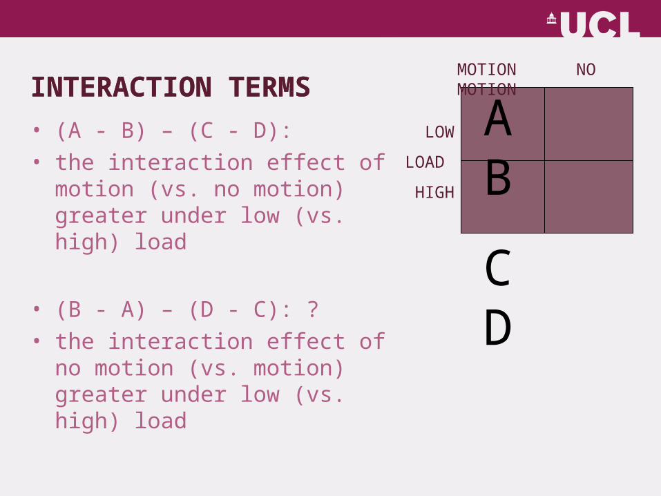
INTERACTION TERMS

A B

C D

LOW

LOAD

HIGH

MOTION NO MOTIONINTERACTION TERMS

• (A - B) – (C - D): • the interaction effect of motion (vs.

no motion) greater under low (vs. high) load

• (B - A) – (D - C): ?• the interaction effect of no motion

(vs. motion) greater under low (vs. high) load

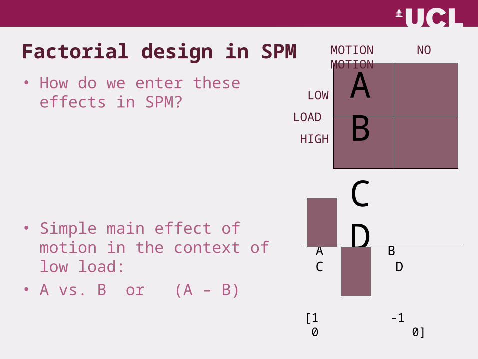
Factorial design in SPM

A B

C D

LOW

LOAD

HIGH

MOTION NO MOTION

A B C D

[1 -1 0 0]

• How do we enter these effects in SPM?

• Simple main effect of motion in the context of low load:

• A vs. B or (A – B)

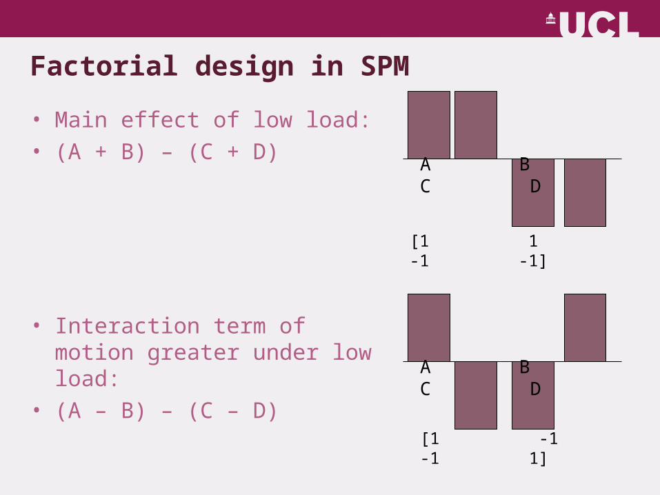
Factorial design in SPM

• Main effect of low load: • (A + B) – (C + D)

• Interaction term of motion greater under low load:

• (A – B) – (C – D)

A B C D

A B C D

[1 -1 -1 1]

[1 1 -1 -1]

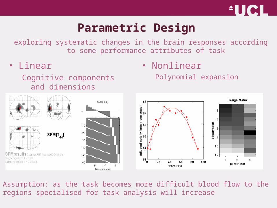
Parametric Design

• LinearCognitive components and

dimensions

• NonlinearPolynomial expansion

Assumption: as the task becomes more difficult blood flow to the regions specialised for task analysis will increase

exploring systematic changes in the brain responses according to some performance attributes of task

Overview

• Experimental Design– Types of Experimental Design– Timing parameters – Blocked and Event-Related Design

• Design Efficiency– Response vs Baseline (signal-processing)– Response 1 - Response 2 (statistics)

Timing Parameters – Blocked Design

• It involves presenting two conditions – an activation (A) condition and a baseline (B) condition. Each condition is presented for an identical epoch of time.

Task A Task B Task A Task B Task A Task B Task A Task B

Task A Task BREST REST Task A Task BREST REST

What baseline should you choose?

• Task A vs. Task B– Example: Squeezing Right Hand vs. Left Hand– Allows you to distinguish differential activation between

conditions– Does not allow identification of activity common to both tasks

• Can control for uninteresting activity

• Task A vs. No-task– Example: Squeezing Right Hand vs. Rest– Shows you activity associated with task– May introduce unwanted results

Choosing Length of Blocks

• Longer blocks allow for stability of extended patterns of

brain activation.

• Shorter blocks allow for more transitions between tasks.

– Task-related variability increases with increasing

numbers of transitions

Pros and Cons of Blocked Design

Pros:• Avoid rapid task-switching (e.g. patients)• Fast and easy to run;• Good signal to noise ratio

Cons:• Expectation• Habituation• Signal drift• Poor choice of baseline may preclude meaningful conclusions• Many tasks cannot be conducted repeatedly

Timing Parameters – Event-Related Design

• It allows different trials or stimuli to be presented in arbitrary sequences.

• Jittering events can reduce possibility of correlated regressors – increased efficiency

time

Pros and Cons of Event-Related Design

Pros:

• Real world testing

• Eliminate predictability of block designs (e.g. expectation);

• Can look at novelty and priming;

• Can look at temporal dynamics of response.

Cons:• Low statistical power (small signal change)• More complex design and analysis (esp. timing and baseline issues).

Overview

• Experimental Design– Types of Experimental Design– Timing parameters – Blocked and Event-Related Design

• Design Efficiency– What is efficiency– Signal Processing perspective– General Advice

Efficiency is…

• … a numerical value which reflects the ability of

your design to detect the effect of interest.

Efficiency is…

• … a numerical value which reflects the ability of

your design to detect the effect of interest.

• General Linear Model: Y = X . β + ε

Data Design Matrix Parameters error

• Efficiency (e) is the ability to estimate β, given the design matrix X

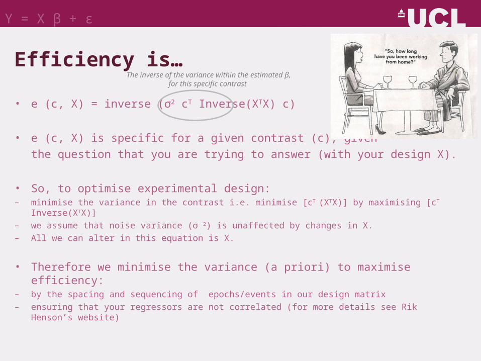
Efficiency is…

• e (c, X) = inverse (σ2 cT Inverse(XTX) c)

• e (c, X) is specific for a given contrast (c), given

the question that you are trying to answer (with your design X).

• So, to optimise experimental design: – minimise the variance in the contrast i.e. minimise [cT (XTX)] by maximising [cT Inverse(XTX)]

– we assume that noise variance (σ 2) is unaffected by changes in X.

– All we can alter in this equation is X.

• Therefore we minimise the variance (a priori) to maximise efficiency:– by the spacing and sequencing of epochs/events in our design matrix

– ensuring that your regressors are not correlated (for more details see Rik Henson’s website)

The inverse of the variance within the estimated β, for this specific contrast

Y = X β + ε

Background: terminology

• Trial - replications of a condition

• A trial consists of one or more components, that may be:

– “events” or “impulses” - brief bursts of neural activity

– “epochs” - periods of sustained neural activity

• SOA (Stimulus Onset Asynchrony) - time between the onsets of components. Also

referred to as the ITI (inter-trial interval).

• ISI (Inter-Stimulus Interval) - time between offset of one component and onset of next

• SOA = ISI + Stimulus Duration

• For events: SOA = ISI (as events are assumed to have zero duration)

Signal Processing

• Signal processing is the analysis, interpretation, and manipulation of signals.

• Given that we can treat fMRI volumes as time series (for each voxel) it is useful to adopt a

signal-processing perspective.

• Using a “linear convolution” model, the predicted fMRI series is obtained by convolving a

neural function (e.g. stimulus function) was an assumed IR.

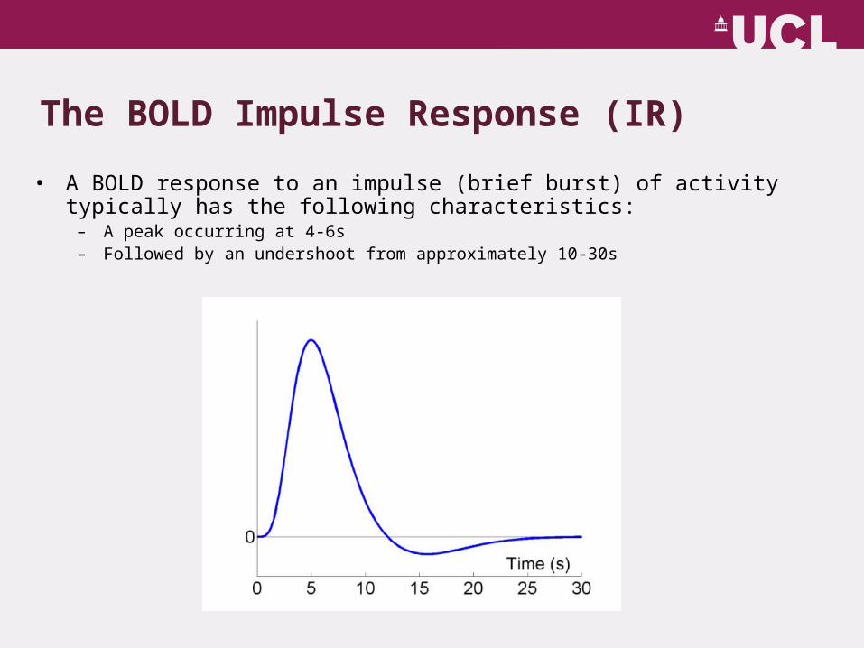
The BOLD Impulse Response (IR)

• A BOLD response to an impulse (brief burst) of activity typically has the following characteristics:

– A peak occurring at 4-6s– Followed by an undershoot from approximately 10-30s

=

Fixed SOA = 16s

Not particularly efficient…

Stimulus (“Neural”) HRF Predicted Data

=

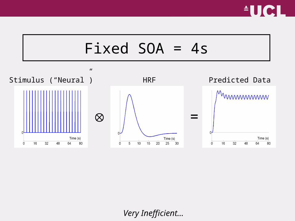
Fixed SOA = 4s

Very Inefficient…

Stimulus (“Neural”) HRF Predicted Data

=

Randomised, SOAmin= 4s

More Efficient, despite using only half as many stimuli as previous…

Stimulus (“Neural”) HRF Predicted Data

=

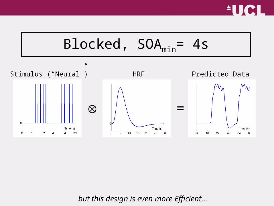
Blocked, SOAmin= 4s

but this design is even more Efficient…

Stimulus (“Neural”) HRF Predicted Data

Background: terminology

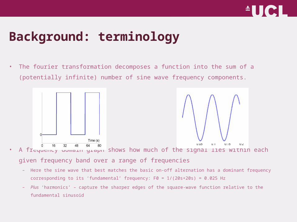
• The fourier transformation decomposes a function into the sum of a (potentially infinite)

number of sine wave frequency components.

• A frequency domain graph shows how much of the signal lies within each given frequency

band over a range of frequencies

– Here the sine wave that best matches the basic on-off alternation has a dominant frequency corresponding to its

‘fundamental’ frequency: F0 = 1/(20s+20s) = 0.025 Hz

– Plus ‘harmonics’ – capture the sharper edges of the square-wave function relative to the fundamental sinusoid

0 100 200 300-1

-0.5

0

0.5

1

0 50 100 1500

20

40

60

80

100

0 50 100 1500

20

40

60

80

100

0 100 200 300-1

-0.5

0

0.5

1

0 100 200 300-1

-0.5

0

0.5

1

0 50 100 1500

20

40

60

80

100

0 50 100 1500

20

40

60

80

100

0 100 200 300-1

-0.5

0

0.5

1

0 100 200 300-1

-0.5

0

0.5

1

0 50 100 1500

20

40

60

80

100

0 50 100 1500

20

40

60

80

100

0 100 200 300-1

-0.5

0

0.5

1

0 100 200 300-1

-0.5

0

0.5

1

0 50 100 1500

20

40

60

80

100

0 50 100 1500

20

40

60

80

100

0 100 200 300-1

-0.5

0

0.5

1

=

Blocked, epoch = 20s

=

• A convolution in time is equivalent to a multiplication in frequency space• In this way the transformed IR acts as a filter: passes low frequencies but attenuates higher frequencies.

Stimulus (“Neural”) HRF Predicted Data

=

Blocked, epoch = 20s

=

Efficient design as most of the signal is ‘passed’ by the IR filter

Stimulus (“Neural”) HRF Predicted Data

So what is the most efficiency design of all…

Sinusoidal modulation, f = 1/33s

=

The most efficient design of all!

Stimulus (“Neural”) HRF Predicted Data

Highpass Filtering

• fMRI noise tends to have two components:

– Low frequency ‘1/f’ noise e.g. physical (scanner drifts);

physiological [cardiac (~1 Hz), respiratory (~0.25 Hz)]

– Background white noise

• Highpass filters aims to maximise the loss of noise but minimise the loss of signal.

• We apply the highpass filter to the lowpass filter inherent in the IR to creast a single ‘band-

pass’ filter (or ‘effective HRF’).

=

“Effective HRF” (after highpass filtering) (Josephs & Henson, 1999)

Blocked (80s), SOAmin=4s, highpass filter = 1/120s

Don’t have long (>60s) blocks!

=

Stimulus (“Neural”) HRF Predicted Data

Randomised, SOAmin=4s, highpass filter = 1/120s

=

=

(Randomised design spreads power over frequencies)

Stimulus (“Neural”) HRF Predicted Data

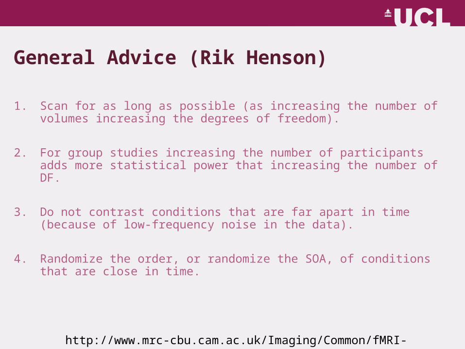
General Advice (Rik Henson)

1. Scan for as long as possible (as increasing the number of volumes increasing the degrees of freedom).

2. For group studies increasing the number of participants adds more statistical power that increasing the number of DF.

3. Do not contrast conditions that are far apart in time (because of low-frequency noise in the data).

4. Randomize the order, or randomize the SOA, of conditions that are close in time.

http://www.mrc-cbu.cam.ac.uk/Imaging/Common/fMRI-efficiency.shtml

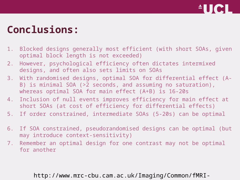
Conclusions:

1. Blocked designs generally most efficient (with short SOAs, given optimal block length is not exceeded)

2. However, psychological efficiency often dictates intermixed designs, and often also sets limits on SOAs

3. With randomised designs, optimal SOA for differential effect (A-B) is minimal SOA (>2 seconds, and assuming no saturation), whereas optimal SOA for main effect (A+B) is 16-20s

4. Inclusion of null events improves efficiency for main effect at short SOAs (at cost of efficiency for differential effects)

5. If order constrained, intermediate SOAs (5-20s) can be optimal

6. If SOA constrained, pseudorandomised designs can be optimal (but may introduce context-sensitivity)

7. Remember an optimal design for one contrast may not be optimal for another

http://www.mrc-cbu.cam.ac.uk/Imaging/Common/fMRI-efficiency.shtml

Useful links and thanks

• Antoinette Nicolle• http://imaging.mrc-cbu.cam.ac.uk/imaging/Design

Efficiency• Nick and Edoardo’s slides from MfD 2008