experimental determination of dislocation densities in
TRANSCRIPT

Arthur Fuchs, BSc
Experimental determination of dislocation densities in martensitic steels
to achieve the university degree of
MASTER'S THESIS
Master's degree programme: Advanced Materials Science
submitted to
Graz University of Technology
Univ.-Prof. Dipl.-Ing. Dr.techn. Bernhard Sonderegger
Institute of Materials Science, Joining and Forming
Diplom-Ingenieur
Supervisor
Graz, March 2018

AFFIDAVIT
I declare that I have authored this thesis independently, that I have not used other
than the declared sources/resources, and that I have explicitly indicated all ma-
terial which has been quoted either literally or by content from the sources used.
The text document uploaded to TUGRAZonline is identical to the present master‘s
thesis dissertation.
Date Signature

Diploma Thesis Arthur Fuchs
Acknowledgements
First of all, I would like to thank my supervisor Univ.-Prof. Dipl.-Ing. Dr.techn. Bernhard Sondereggerfor his guidance. I really appreciate giving me my space but immediately being there when I neededdirections.
In addition, I would like to thank all my colleagues from the IMAT for their support and their friendlyattitude.
Furthermore, great appreciation is directed towards the XRD group of the Institute of Solid StatePhysics (TU Graz), especially Ao.Univ.-Prof. Dipl.-Ing. Dr.techn. Roland Resel, for the considerableamount of measurement time granted and for teaching me how to operate the X-ray diffractometer inthe first place.
Special thanks go to the Institute of Materials Physics (TU Graz), especially Dipl.-Ing. BSc RobertEnzinger, for doing the dilatometer measurements and redoing them under argon atmosphere, as soonas we realized that evaporation of Cr is a problem under high vacuum.
I would also like to thank my family, especially my parents and my girlfriend, for their great support.And finally to all my friends: Thanks to those of you who studied with me for exams, those of youwho prevented me from studying when I overdid it and those who did both!
Thank you very much, everyone!
Arthur Fuchs
Graz, March 2018.

Diploma Thesis Arthur Fuchs
1 Abstract
This work deals with the measurement of dislocation densities in complex martensitic alloys. In thesematerials, dislocation motion is responsible for plastic deformation and thus determines propertiessuch as yield strength or creep resistance. Up to now, there has been no physically justified standardprocedure to determine this property with good statistical significance and reasonable experimentaleffort. X-Ray diffraction (XRD) potentially is such a method, combining low experimental cost withsufficient sample volume. Nevertheless, the complexity of the microstructure interferes with a straight-forward application of standard methods usually applied in other, less complex, materials.In this work, conventional XRD-methods are adapted to a martensitic 9% Cr steel (P91). The basicphysical concept is simple: An (ideally) monochromatic and parallel X-ray beam interacts with thecrystal structure of the sample, the diffraction angle(s) Θ is a measure of the interatomic distance(s)according to Bragg’s law. The broadening of the diffraction peak results from (i) properties of theexperimental equipment and (ii) the microstructure of the sample. (i) is referred to as instrumentalbroadening and includes properties of the beam, the slits and the lenses, (ii) comprises any effectleading to local deviations from the ideal lattice constant, which is mostly dislocations and innerboundaries of any type.For the measurement, a PANalytical Empyrean XRD with Cu Kα radiation was used. The sampleswere a NIST LaB6 standard and seven P91 samples (austenitized (1), austenitized and heat treated(2-7)).In a first step, the instrumental broadening was characterized by measurement of the LaB6 standard.With this reference, the data from the steel samples could be de-convoluted into sample- and instru-mental broadening. Finally, the sample broadening was split into microstrains and broadening due tocoherent domain size. For this procedure, some established methods like ”Williamson-Hall”, ”mod-ified Williamson-Hall”, ”Warren-Averbach” and ”double-Voigt” are compared qualitatively to eachother. Furthermore, the frequently used “modified Warren Averbach” method and the most commonmistake with this method is discussed in detail. A workaround, by introducing the contrast factor ofdislocations into the double-Voigt method, is presented. In the modified Williamson-Hall and mod-ified Warren-Averbach methods, the dislocation density is calculated assuming, that all microstrain-inducing defects except dislocations are negligible.Exemplarily, the results are compared to findings from high-precision dilatometry tests and the resultsdiffer by less than a factor of two.
II

Diploma Thesis Arthur Fuchs
Contents
1 Abstract II
2 Parameter List V
3 Introduction 13.1 Task . . . . . . . . . . . . . . . . . . . . . . . . . . . . . . . . . . . . . . . . . . . . . . 1
4 Basics 24.1 General information about X-ray diffraction . . . . . . . . . . . . . . . . . . . . . . . . 2
4.1.1 Generation of X-rays . . . . . . . . . . . . . . . . . . . . . . . . . . . . . . . . . 24.1.2 Bragg’s law . . . . . . . . . . . . . . . . . . . . . . . . . . . . . . . . . . . . . . 34.1.3 Setup of an X-ray diffractometer . . . . . . . . . . . . . . . . . . . . . . . . . . 44.1.4 Peak characteristics . . . . . . . . . . . . . . . . . . . . . . . . . . . . . . . . . 54.1.5 Peak-shapes in XRD-measurements . . . . . . . . . . . . . . . . . . . . . . . . 6
4.2 Instrumental broadening correction . . . . . . . . . . . . . . . . . . . . . . . . . . . . . 74.2.1 Cauchy-/Gauss deconvolution . . . . . . . . . . . . . . . . . . . . . . . . . . . . 74.2.2 Voigt deconvolution . . . . . . . . . . . . . . . . . . . . . . . . . . . . . . . . . 74.2.3 Stokes deconvolution . . . . . . . . . . . . . . . . . . . . . . . . . . . . . . . . . 8
4.3 General information about size-/strain analysis . . . . . . . . . . . . . . . . . . . . . . 84.4 Williamson-Hall method . . . . . . . . . . . . . . . . . . . . . . . . . . . . . . . . . . . 84.5 Warren-Averbach method . . . . . . . . . . . . . . . . . . . . . . . . . . . . . . . . . . 104.6 Modified Williamson-Hall and modified Warren-Averbach approach . . . . . . . . . . . 124.7 Groma’s method . . . . . . . . . . . . . . . . . . . . . . . . . . . . . . . . . . . . . . . 124.8 Double-Voigt . . . . . . . . . . . . . . . . . . . . . . . . . . . . . . . . . . . . . . . . . 134.9 Dilatometry . . . . . . . . . . . . . . . . . . . . . . . . . . . . . . . . . . . . . . . . . . 13
5 Experimental 145.1 Mathematical considerations for data processing . . . . . . . . . . . . . . . . . . . . . 14
5.1.1 Combination of modified Williamson-Hall and modified Warren-Averbach . . . 145.1.2 Combination of modified Warren-Averbach and Double-Voigt . . . . . . . . . . 16
5.2 Sample preparation . . . . . . . . . . . . . . . . . . . . . . . . . . . . . . . . . . . . . . 195.3 X-ray diffraction . . . . . . . . . . . . . . . . . . . . . . . . . . . . . . . . . . . . . . . 195.4 Dilatometry . . . . . . . . . . . . . . . . . . . . . . . . . . . . . . . . . . . . . . . . . . 205.5 Data processing . . . . . . . . . . . . . . . . . . . . . . . . . . . . . . . . . . . . . . . . 20
5.5.1 Matlab programs for data processing . . . . . . . . . . . . . . . . . . . . . . . . 21
6 Results 256.1 X-ray diffraction . . . . . . . . . . . . . . . . . . . . . . . . . . . . . . . . . . . . . . . 256.2 Dilatometry . . . . . . . . . . . . . . . . . . . . . . . . . . . . . . . . . . . . . . . . . . 30
7 Data Analysis and Discussion 317.1 Fitting of XRD peaks . . . . . . . . . . . . . . . . . . . . . . . . . . . . . . . . . . . . 317.2 Separation of size- and strainbroadening . . . . . . . . . . . . . . . . . . . . . . . . . . 34
7.2.1 Williamson-Hall method (also see chapter 4.4): . . . . . . . . . . . . . . . . . . 347.2.2 Modified Williamson-Hall technique (also see chapter 4.6): . . . . . . . . . . . . 357.2.3 Warren-Averbach method (also see chapter 4.5): . . . . . . . . . . . . . . . . . 36
7.3 Modified Warren-Averbach method (also see chapter 4.6): . . . . . . . . . . . . . . . . 377.3.1 Double-Voigt method (also see chapter 4.8): . . . . . . . . . . . . . . . . . . . . 37
III

Diploma Thesis Arthur Fuchs
7.4 Calculation of dislocation densities . . . . . . . . . . . . . . . . . . . . . . . . . . . . . 387.4.1 Calculation of dislocation densities according to the contrast-corrected double-
Voigt method . . . . . . . . . . . . . . . . . . . . . . . . . . . . . . . . . . . . . 397.5 Dilatometry . . . . . . . . . . . . . . . . . . . . . . . . . . . . . . . . . . . . . . . . . . 417.6 Comparison of results . . . . . . . . . . . . . . . . . . . . . . . . . . . . . . . . . . . . 42
8 Conclusion 44
9 Appendix 499.1 XRD measurement specifications . . . . . . . . . . . . . . . . . . . . . . . . . . . . . . 499.2 Determining γ in the modified Warren-Averbach method . . . . . . . . . . . . . . . . . 539.3 Plots of data fits . . . . . . . . . . . . . . . . . . . . . . . . . . . . . . . . . . . . . . . 53
9.3.1 LaB6 standard . . . . . . . . . . . . . . . . . . . . . . . . . . . . . . . . . . . . 539.3.2 Steel samples . . . . . . . . . . . . . . . . . . . . . . . . . . . . . . . . . . . . . 60
9.4 Fit results . . . . . . . . . . . . . . . . . . . . . . . . . . . . . . . . . . . . . . . . . . . 629.5 Determination of q . . . . . . . . . . . . . . . . . . . . . . . . . . . . . . . . . . . . . . 729.6 Matlab codes . . . . . . . . . . . . . . . . . . . . . . . . . . . . . . . . . . . . . . . . . 73
9.6.1 Peak fitting . . . . . . . . . . . . . . . . . . . . . . . . . . . . . . . . . . . . . . 739.6.2 pseudoVoigtAsym C G separate . . . . . . . . . . . . . . . . . . . . . . . . . . 739.6.3 pseudoVoigtAsym separate . . . . . . . . . . . . . . . . . . . . . . . . . . . . . 769.6.4 LaB6 peak fit . . . . . . . . . . . . . . . . . . . . . . . . . . . . . . . . . . . . . 789.6.5 Steel peak fit . . . . . . . . . . . . . . . . . . . . . . . . . . . . . . . . . . . . . 889.6.6 LaB6 exp fit . . . . . . . . . . . . . . . . . . . . . . . . . . . . . . . . . . . . . 979.6.7 mWH mWA . . . . . . . . . . . . . . . . . . . . . . . . . . . . . . . . . . . . . 100
IV

Diploma Thesis Arthur Fuchs
2 Parameter List
Table 1: Parameter List
Parameter Meaning Definition in:
α Parameter: α = (KD)2 eq. 34a
β Integral breadth. Subscripts provide more information eq. 2βS Integral breadth due to crystallite size eq. 13βD Integral breadth due to microstrains eq. 14βsample Total integral breadth due to crystallite size and micro-
strainseq. 8
βinstrument Integral breadth due to instrumental broadening eq. 8βobserved Integral breadth observed when measuring the strain-
broadened sampleeq. 8
γ Parameter: γ = πMb2ρ2 eq. 34b
< ǫ2(L) > Mean-square-strain eq. 23
η Microstrains: η = ∆dd
eq. 14aΘ Diffraction angle fig. 3Θ0 Bragg angle of Kα reflection maximum eq. 3λ Used X-ray wavelength eq. 1ρ Dislocation density eq. 25A Real part of the curves’ Fourier series eq. 20AD
n Distortion coefficient of A eq. 20AS
n Size coefficient of A eq. 20
B Parameter: B = πb2
2 eq. 27aC Average dislocation contrast factor eq. 25Ch00 Dislocation contrast factor for (h00)-planes eq. 33C(2Θ) Cauchy function eq. 3D Crystallite size eq. 13F Constant for dislocations interactions; in this work F = 1 eq. 45f(x), F (x) Pure-specimen (physically) broadened profile and its Fourier
transformeq. 7
g(x), G(x) Instrumentally broadened profile and its Fourier transform eq. 7G(2Θ) Gauss function eq. 4h(x), H(x) Observed broadened profile and its Fourier transform eq. 7
H Parameter: H2 = h2k2+h2l2+k2l2
h2+k2+l2eq. 33a
K Shape factor; can be assumed as ≈ 1 eq. 13L Fourier length L = n · a eq. 21M and M ′ Parameters depending on the effective outer cutoff radius of
dislocationseq. 25
PV II(2Θ) Pearson VII function eq. 6Q A correlation factor eq. 25Re Outer cut-off radius for dislocations: Re ≈ 1
2ρ eq. 27
V and ∆V Volume and volume change of dilatometry sample eq. 31V (2Θ) Voigt function eq. 5W Full-width-at-half-maximum sec. 4.1.4
X Parameter: X = (∆g)2−α
g2eq. 36
Y Parameter: Y = ρBL2 ln(Re
L) eq. 39
V

Diploma Thesis Arthur Fuchs
a Unit of Fourier length in direction of the diffraction vectorg
eq. 21
b Burgers Vector eq. 25d Interatomic distance fig. 3
g Variable in reciprocal space: g = 2sin(Θ)λ
= 1d
eq. 15a and 25
∆g Parameter: ∆g =βsample2cos(Θ)
λeq. 25
g0 Some constant eq. 28h, k, l Miller indicesj Constant that depends on the lattice; j = 14.4 for bcc eq. 45k Slope for a linear y = kx+ d functionl and ∆l Length and length change of dilatometry sample eq. 31m Shape factor for Pearson VII function eq. 6n Some integerq Parameter depending on elastic constants and dislocation
charactereq. 33
vdisl Specific excess free volume of dislocations eq. 32ax General variable, usually either x = Θ or x = g eq. 7⋆ Convolution: g(x) ⋆ f(x) =
∫
g(z)f(x− z) dzSubscriptsf Denotes the pure-specimen (physically) broadened profilef(η) Wilkens function eq. 26g Denotes the instrumentally broadened profileh Denotes the observed profile (instrumental and physical
broadened)C Denotes the Cauchy component of the Voigt functionD Denotes the distortion relation of a parameterG Denotes the Gaussian component of the Voigt functionS Denotes the crystallite size relation of a parameter
VI

Diploma Thesis Arthur Fuchs
3 Introduction
In most metals, plastic deformation is determined by the movement of dislocations and propertieslike yield strength and creep behaviour depend on them. For martensitic 9 % Cr steels (e.g. P91),especially the creep behaviour is crucial. Until now mostly TEM, EBSD and X-ray diffraction wereused to determine dislocation densities. TEM has the disadvantages of very high costs combined withvery bad statistical evidence and EBSD measures geometrically necessary- and wall-dislocations only.Thus, only X-ray diffraction combines moderate experimental costs with sufficient volumes for goodstatistics. This is why many papers already used this technique (e.g. [1] [2]).The basics of dislocation density measurements via XRD go back to the well known Scherrer formulafrom 1918 ( [3]): Scherrer noted that not only the position of an XRD peak is important (Bragg’slaw), but its broadness is influenced by the material’s microstructure. He then denotes all peakbroadening to the size of coherently diffracting domains. In 1944, Stokes and Wilson noted that peakbroadening can be also caused by microstrains and developed a formula to quantify this ”apparentstrain” [4]. Later, Williamson and Hall combined these two approaches in their Williamson-Hallmethod to separate size- and strainbroadening [5]. This method is still very popular nowadays, eventhough its limitation to rough estimations has been stated multiple times (e.g. [6]). Later, the morefundamental but also more time-consuming Warren-Averbach approach [7] was published, which isalso still used nowadays. The latest milestone for dislocation density measurements was done by T.Ungar at around 2000: He assumed all microstrains other than those of dislocations are negligible andthus published his modified Williamson-Hall- and modified Warren-Averbach approach [8]. Since thattime, many authors used this techniques to evaluate dislocation densities and coherent domain sizes,often neglecting limitations and uncertainties. A critical review about using integral breath methodscarelessly, especially the modified Williamson-Hall technique, is done in [9].Nowadays there are two general approaches to apply the methods mentioned above to XRD data:
• Rietveld, Whole-profile-fitting,...: The first of this methods, the ”Rietveld refinement” [10]was first introduced in the late 60s. In general, these methods share the same basic principle: Allphenomena that change peak properties have to be described in mathematical models. Then,the whole profile measured is fitted according to these models. The differences between Rietveld,Whole-profile-fitting,... are solely the included models. These are very powerful techniques ingeneral, but the operator needs to be very experienced because one wrong input afterwards maybe ”corrected” by other wrong results and controlling these programs is difficult (”black boxes”).
• Single peak fitting: In these methods, every peak is fitted separately and the mathematicalmodels describing the microstructures are applied afterwards. This has many advantages whentesting different data processing models, because the CPU-intensive fitting procedure is done a
priori. Furthermore, controlling the data analysis routines step-by-step is much easier. In thiswork, only single peak fitting methods are used.
3.1 Task
Aim of this work was to evaluate the capabilities and limitations of dislocation density measurementswith X-ray diffraction on martensitic 9 % Cr steels (P91). To do so, methods to extract the instrumen-tal broadening such as Cauchy-, Gauss-, Voigt- and Stokes deconvolution were tested and the mostpopular methods of data processing were evaluated: Williamson-Hall-, Warren-Averbach-, double-Voigt-, modified Williamson-Hall- and m. Warren-Averbach method. Groma’s peak tail analysis [11]could not be used, as the measured data did not meet the required quality for this method.
To check the reliability of the XRD methods, dilatometry as an alternative method was also tested.
1

Diploma Thesis Arthur Fuchs
4 Basics
4.1 General information about X-ray diffraction
4.1.1 Generation of X-rays
The generation of X-rays is well-described in many books, e.g. [12] and [13] . Nevertheless, becausemany problems of this work are due to its specifics, a short overview is given in the following.There are various ways of producing X-rays. The most important ones are synchrotron radiation,braking radiation (”Bremsstrahlung”) and characteristic radiation. For this thesis, only braking radi-ation and characteristic radiation are important. The origin for both of them can be described by thebombardment of a metallic target with electrons:
• Braking radiation: The electrons are rapidly slowed down when they hit the target, whichincludes a loss in energy. Most of this energy is transferred into heat, but some of it is dispersedin form of radiation. This radiation is called ”braking radiation” or ”Bremsstrahlung”. Itsemission spectrum is continuous and the intensity increases with increasing acceleration voltage.At the same time, the minimum wavelength λmin decreases with increasing acceleration voltage.
• Characteristic radiation: If an element is bombarded with high energy particles, in this caseelectrons, there is the possibility that a bound electron from an inner shell is excited and anelectron from an outer shell takes its place. As the electron falls to the inner shell, it emits anX-ray with a very specific wavelength, corresponding to the energy gap between the two electronshells. This radiation can have several wavelengths, but its spectrum is discontinuous. Eventhough the intensities of these X-rays are usually much higher than the intensities of the brakingradiation, there still is a contribution of the braking radiation. This results in a continuousbackground radiation.
A typical spectrum of a molybdenum anode is shown in fig. 1 . The continuous background correspondsto braking radiation, the Kα and Kβ peaks correspond to characteristic molybdenum radiation.
Figure 1: Example for the spectrum of a molybdenum anode. The continuous part corresponds tothe braking radiation, the two sharp peaks are characteristic radiation. [Fig.1]
2

Diploma Thesis Arthur Fuchs
The setup for a typical X-ray tube (in this case a ”Coolidge tube”) is shown in fig. 2 .
Figure 2: Setup for a ”Coolidge tube” as typical example for an X-ray source. [Fig.2]
In most cases, the filament is made of tungsten. This together with the geometry shown in fig. 2 canexplain two major problems when performing X-ray diffraction (XRD).
1. The source is not perfectly dot-like. This together with not perfect slits, lenses, monochroma-tors,... lead to the so called ”instrumental broadening”. 1
2. Tungsten from the filament evaporates and condenses again, especially at the anode and wallsof the tube. This deposition on the anode leads to absorption of some of the emitted X-rays andto the presence of parasitic X-rays 2.
4.1.2 Bragg’s law
When the X-rays from the tube get reflected by a material (sample), they first interact with thissample, then with each other (=interference). This can be described by Bragg’s law: [15]
2d sin(Θ) = nλ (1)
with the inter-atomic distance d, the X-ray wavelength λ and a positive integer n. Note that perfectlynarrow peaks only occur for defect-free (includes not distorted!) crystals (no changes in the inter-atomic distance) A visualization of Bragg’s law can be seen in fig. 3:
Figure 3: Bragg’s law: Constructive interference is only possible, if wave maxima of both waves areat the same position. This is the case, when the path difference (= 2d sin(Θ)) equals tonλ. [Fig.3]
1A detailed evaluation of instrumental broadening factors is done in chapter 3.1 of [14]2In general, all not coherent with the main source and not wanted X-rays are called ”parasitic”
3

Diploma Thesis Arthur Fuchs
4.1.3 Setup of an X-ray diffractometer
The general setup of an X-ray diffractometer is shown in fig. 4 .
Figure 4: General setup of an X-ray diffractometer.Divergence slit... limits horizontal divergenceMask... guarantees, that the irradiated area is smaller than the sampleAnti-scatter-slit... filters stray lightSoller-slit... prevents vertical beam divergenceMonochromator... guarantees, that only selected wavelengths reach the detector
First, the X-rays have to pass a divergence slit, that limits horizontal beam divergence. Limiting thebeam divergence too much results in very weak intensities. After the divergence slit, a mask guaranteesthat only the sample is irradiated, even at smaller 2Θ angles. After the sample, an anti-scatter-slitfilters stray light and a soller-slit prevents vertical beam divergence (it is quite common to have an-other soller-slit directly after the X-ray tube, before the beam passes the divergence slit). Finally, amonochromator suppresses all wavelengths except the Kα radiation, which also reduces backgroundradiation originating within the sample. [12] [13]A typical XRD-measurement detects angle-dependent diffracted intensities. There are several mea-surement methods that could be used described in [12]. Fig. 4 shows a normal Θ/2Θ-measurementas used in this work.More detailed descriptions on basics of X-ray diffraction can be found in books, e.g. [16].
4

Diploma Thesis Arthur Fuchs
4.1.4 Peak characteristics
As described in the next section, there are several ways to model peak shapes. To nevertheless be ableto model universally applicable mathematical methods, some unique peak features were specified:
Half-width-at-half-maximum:The half-width-at-half-maximum (HWHM) gives a good description of the peak broadness. Oneadvantage is, that the method is applicable for any fixed, symmetric random peak shape. One disad-vantage is that not the full information of the peak is used. This makes it inaccurate for comparisons ofasymmetric and differently shaped peaks (e.g. if the Cauchy/Gauss ratio of Pearson VII or Voigt peakschange). In some cases, the peak broadness is described by the full-width-at-half-maximum (FWHM),that is two times the half-width-at-half-maximum. Both full- and half-width-at-half-maximum areused for rough estimations and quick data analysis.Fig. 5 graphically shows the half-width-at-half-maximum:
xx1 x2
f(x)
fmax
1/2*fmax
Figure 5: Graphical description of the half-width-at-half-maximum (HWHM)
Integral breadth:For more precise analysis, the integral breadth (IB) should be used. In the following, the integralbreadth is referred to as β and it is defined in eq. 2:
β =Peak Area
Peak height(2)
As with the FWHM or the HWHM, the integral breadth method can be applied to any peak shape.If the background level is evaluated carefully, it is much more robust to comparing differently shapedand asymmetric peaks than FWHM/HWHM.
5

Diploma Thesis Arthur Fuchs
4.1.5 Peak-shapes in XRD-measurements
The peak shape of an XRD Θ/2Θ-measurement does not fit into a single scheme and can only bedetermined empirically. For rough estimations, Cauchy 3 (eq. 3) or Gaussian shapes (eq. 4) canbe used. Usually, neither of these describes the measured peak accurately. Mostly acknowledgedfunctions are the Voigt-function (eq. 5) and the Pearson VII function (eq. 6). [14]
Cauchy function: [14]
C (2Θ) =2
πW
1 +
4(√
2− 1)
W 2(2Θ− 2Θ0)
2
−1
(3)
with the full-width-at-half-maximum (FWHM) W and the peak maximum (usually of Kalpha1) Θ0.
Gauss function: [14]
G (2Θ) =2
W
√
ln(2)
πexp
[−4 ln(2)
W 2(2Θ− 2Θ0)
2
]
(4)
Voigt function (is a convolution of a Cauchy- and a Gauss function): [14]
V (2Θ) = β−1G Re
erfc
(√π
βG|2Θ− 2Θ0|+ i
βCβG
√π
)
(5)
where:
• Re: real part of a complex function
• erfc: complex error function
• βC and βG: integral breadths of the Gaussian and Lorentzian components
• i: imaginary number
Since convolutions are quite CPU-intensive, most programs use the ”pseudo-Voigt” function, which isa linear combination of a Cauchy- and a Gauss function 4, instead of the Voigt function.
Pearson VII function: [14]
PV II (2Θ) =2√mΓ
(
21
m − 1)
WπΓ (m− 0, 5)
1 +
4(
21
m − 1)
W 2(2Θ− 2Θ0)
2
−m
(6)
where m is a shape factor (m < 1 super-Lorentzian; m = 1 Lorentzian and m >> 1 Gaussian) and Γis the Gamma function.
3Lorentzian and Cauchy function are the same4”pseudo-”Voigt, because the linear combination is an approximation for the Voigt function’s convolution
6

Diploma Thesis Arthur Fuchs
4.2 Instrumental broadening correction
In the last section, peak shapes were discussed. By fitting one of them to the measured data, thediscontinuous sets of data are described by a continuous function. The next step in data analysis is todecompose the peak into different phenomena that contribute to its position, broadness and intensity(in this work, only broadness will play a major role). Note that the peak broadening is dependent onthe diffraction angle 2Θ.In general the observed peak is a convolution of the instrumentally broadened peak and the samplebroadened peak. [17]
h(x) = g(x) ⋆ f(x) (7)
with the observed broadened profile h(x), the instrumentally broadened profile g(x) and the physicallybroadened sample profile f(x).To determine the instrumental broadening only, there are two techniques used frequently:
• Simulation of the instrument with all slits and lenses used.
• Measurement of an external standard without sample broadening, e.g. some NIST standard 5.For reasons of convenience, this is the technique used most.
Depending on the data processing technique used, there are different methods to perform this instrumental-/sample broadening separation, the most important ones described in the following.
4.2.1 Cauchy-/Gauss deconvolution
If the measured XRD peaks can be fitted with either Cauchy- or Gauss peaks, the instrumentalbroadening can be extracted with eq. 8 and eq. 9:
Cauchy: βsample = βobserved − βinstrument (8)
Gauss: β2sample = β2
observed − β2instrument (9)
with the integral breadth observed when measuring the strain-broadened sample βobserved, the integralbreadth due to crystallite size and microstrains βsample and the integral breadth due to instrumentalbroadening βinstrument.
Since peak shapes usually are neither pure Cauchy nor pure Gaussian, the fit quality suffers. Widelyacknowledged peak shapes would be the Voigt profile (convolution of Cauchy and Gauss peaks),the pseudo-Voigt profile (the convolution is approximated by a linear combination of Cauchy andGauss peaks) and the Pearson VII profile (see sec. 4.1.5). The deconvolution of Voigt- (and theirapproximation, the pseudo-Voigt) functions is discussed in the next chapter.
4.2.2 Voigt deconvolution
In the so called double-Voigt approach, both instrument and observed peaks are modelled via Voigt-or pseudo-Voigt functions. Since the convolution of two Voigt functions is also a Voigt function,the Cauchy-/Gaussian parts can be deconvoluted separately and the instrumental broadening can beextracted easily: [18]
βfC = βhC − βgC (10)
β2fG = β2
hG − β2gG (11)
5NIST: National Institute of Standards and Technology. Commonly used standards for XRD applications are NISTSRM 660 (LaB6) and NIST SRM 640 (Si).
7

Diploma Thesis Arthur Fuchs
with the Cauchy and Gaussian parts of the pure-specimen broadened integral breadths βfC and βfG,of the observed integral breadths βhC and βhG and of the instrumentally broadened integral breadthsβgC and βgG.
4.2.3 Stokes deconvolution
Another deconvolution method is the method of Stokes [19]. From eq. 7 follows, that the deconvolutioncan be done quite easily in fourier-space: [19]
F (z) =H(z)
G(z)(12)
F (z), H(z) and G(z) are the Fourier transforms of f(x), h(x) and g(x) (see eq. 7).Transforming F (z) back into real space gives the pure physically broadened profile f(x). The bigadvantage of this method is, that no assumption concerning peak shape have been done so far.
After the pure sample-broadened peak is separated, the size-/strain analysis can be done.
4.3 General information about size-/strain analysis
Most formulas in diffraction theory (like Bragg’s- and Laue’s law) were developed for perfect mono-crystals. In real crystals, the perfect grid of atoms is tilted and bent through imperfections (e.g.clusters of dislocations and twins). This divides the material in many small volumes, where Bragg’slaw can be applied, which are called ”coherent domains”. The domain size is usually called ”crystallitesize”, which is often confused with grain- or subgrain size. These two groups of microstructural featuresare not identical and should not be mixed up. There are however special cases like defect free nanopowders (grain size) and fully recovered fine grained materials (subgrain size), where they are equalto each other.The topic in size-/strain analysis is how to separate the pure specimen-broadened peak into size-effects(coherent domains) and microstrains.
4.4 Williamson-Hall method
Since the Williamson-Hall method assumes Cauchy- or Gaussian peak shapes, usually the methoddescribed in sec. 4.2.1 is used for separation of the instrumental broadening.
A general approach to calculate the crystallite size is the Scherrer-formula: [3]
βS(Θ) =K · λ
D · cos(Θ)(13)
with the integral breadth due to crystallite size βS(Θ), the X-ray wavelength λ, the crystallite size Dand the diffraction angle Θ. The shape factor K can be assumed as ≈ 1.The microstrains can be described by the Stokes-Wilson-formula: [4]
βD(Θ) = η · tan(Θ) (14)
with the integral breadth due to microstrains βD(Θ) and the microstrains
η =∆d
d(14a)
8

Diploma Thesis Arthur Fuchs
in which d is the inter-atomic distance.With
g =2sin(Θ)
λ(15a)
the integral breadth in real space (β(Θ)) can be transformed to reciprocal space (β(g)):
β(g) =β(Θ)cos(Θ0)
λ(15b)
With the Bragg angle of Kα reflection maximum Θ0.
In general the easiest way to differentiate between size and strain broadening is that strain broadeningin reciprocal space is dependent on the diffraction angle Θ and size broadening is not.This implies different Θ dependences of size- and strain broadening in real space. The exact dependenceof the strain broadening on Θ varies with the evaluation model one chooses. [18] Common models are:1) The ”apparent” strain defined by Stokes and Wilson [4] (which corresponds to a maximum strain)that is used in all simplified integral breadth methods e.g. the Williamson-Hall approach. 2) Themean-square strain defined by Warren [20] and used in the Warren-Averbach approach.
G.K. Williamson and W.H. Hall assumed, that either the integral breadths or their squares sum upto the measured peak:
βnsample(Θ) = βn
D(Θ) + βnS(Θ) (16)
where n=1 for pure Cauchy and n=2 for pure Gaussian shapes. With this assumption the authorswere able to combine eq. 13 and eq. 14 6. Using n = 1 (Cauchy only!), eq. 17 is achieved: [5]
βsample(Θ) = βD(Θ) + βS(Θ) = η · tan(Θ) +K · λ
D · cos(Θ)(17)
By multiplying eq. 17 with cos(Θ) one gets eq. 18 [5].Note that this equation is only valid for pure Lorentzian (=Cauchy) peak shapes and that the sizepart of this equation is not dependent on Θ.
βsample(Θ) · cos(Θ) = η · sin(Θ) +K · λD
(18)
By plotting βsample(Θ) · cos(Θ) vs. sin(Θ), the system can be treated as a simple linear equation
y = kx + d (18a)
withk = η (18b)
d =K · λD
(18c)
By doing so, the crystallite size and microstrains can be fitted conveniently, as seen in fig. 6.
6Nowadays, also mixed types, especially βS(Θ) → cauchy and βD(Θ) → gauss are popular.
9
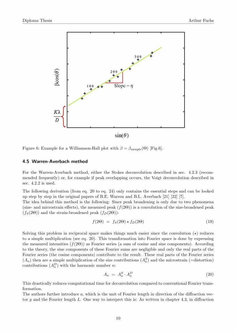
Diploma Thesis Arthur Fuchs
Figure 6: Example for a Williamson-Hall plot with β = βsample(Θ) [Fig.6].
4.5 Warren-Averbach method
For the Warren-Averbach method, either the Stokes deconvolution described in sec. 4.2.3 (recom-mended frequently) or, for example if peak overlapping occurs, the Voigt deconvolution described insec. 4.2.2 is used.
The following derivation (from eq. 20 to eq. 24) only contains the essential steps and can be lookedup step by step in the original papers of B.E. Warren and B.L. Averbach [21] [22] [7].The idea behind this method is the following: Since peak broadening is only due to two phenomena(size- and microstrain effects), the measured peak (f(2Θ)) is a convolution of the size-broadened peak(fS(2Θ)) and the strain-broadened peak (fD(2Θ)):
f(2Θ) = fS(2Θ) ⋆ fD(2Θ) (19)
Solving this problem in reciprocal space makes things much easier since the convolution (⋆) reducesto a simple multiplication (see eq. 20). This transformation into Fourier space is done by expressingthe measured intensities (f(2Θ)) as Fourier series (a sum of cosine and sine components). Accordingto the theory, the sine components of these Fourier sums are negligible and only the real parts of theFourier series (the cosine components) contribute to the result. These real parts of the Fourier series(An) then are a simple multiplication of the size contributions (AS
n) and the microstrain (=distortion)contributions (AD
n ) with the harmonic number n:
An = ASn ·AD
n (20)
This drastically reduces computational time for deconvolution compared to conventional Fourier trans-formation.The authors further introduce a, which is the unit of Fourier length in direction of the diffraction vec-tor g and the Fourier length L. One way to interpret this is: As written in chapter 4.3, in diffraction
10

Diploma Thesis Arthur Fuchs
theory materials can be considered consisting of coherent diffracting domains. According to Warrenand Averbach, each of these domains again is considered consisting of columns of cells along a specificdirection. This grid then has the length a and the distance between cell pairs (L) is defined in eq.21:
L = n · a (21)
With this, An = A(n) can be converted to A(L) and eq. 22 is achieved:
ln[
A (L)]
= ln[
AS (L)]
+ ln[
AD (L)]
= ln[
AS (L)]
+ ln{
< exp[
2πigLǫ (L)]
>}
(22)
with the microstrain ǫ(L).For not too large L and a Gaussian strain distribution the following approximation can be made:
< exp[
2πigLǫ (L)]
>≈ exp[
−2π2g2L2 < ǫ2 (L) >]
(23)
Where < ǫ2(L) > is the so called ”mean-square-strain” 7. It is the square of the non-uniform strainaveraged over the distance L.Inserting eq. 23 into eq. 22, the seminal Warren-Averbach relation is achieved: [21] [22] [7]
ln[
A (L)]
= ln[
AS (L)]
− 2π2g2L2 < ǫ2 (L) > (24)
By plotting ln[
A (L)]
vs. the square of the diffraction vector, g2, one gets the Warren-Averbach plotshown in fig. 7.
Figure 7: Example for a Warren-Averbach plot. The intercepts with the y-axis yield the size coeffi-cients and the slopes the mean-square strains < ǫ2 (L) > (compare with eq. 24 ).
7also referred to as emss
11

Diploma Thesis Arthur Fuchs
4.6 Modified Williamson-Hall and modified Warren-Averbach approach
T. Ungar noted, that most of the deviations from a straight line in the Williamson-Hall plot can bedue to simple phenomena [8]. For example considering strain broadening solely due to dislocations,a contrast factor for dislocations (C) should be included to account for differences in intensity. Fur-thermore, a logarithmic series expansion of the Fourier coefficients should be done. Doing this, themodified Williamson-Hall equation is given in eq. 25: [8]
∆g ∼= K
D+
√
πMb2
2· ρ · g
√C +
πM ′b2
2·√
Q · g2C (25)
With shape factor K (≈ 1), the crystallite size D, the Burgers Vector b, the dislocation density ρ,a correlation factor Q and the average dislocation contrast factor C (see eq. 33 ). For a detaileddescription of the dislocation contrast factor see [8] at p. 5. M and M ′ are parameters depending onthe effective outer cutoff radius of dislocations (Re) and the dislocation density (for determination ofdislocation densities, it is not necessary to evaluate these values). Parts of eq. 18 were merged to
∆g =βsample(Θ)2cos(Θ)
λ(25a)
g =2sin(Θ)
λ(25b)
T. Ungar also applied this approach to the Warren-Averbach equation. For the microstrains, eq. 26was used:
< ǫ2(L) > =
(
b
2π
)2
πρf(η)C (26)
where f(η) is the Wilkens function. Approximating the Wilkens function in a series expansion, trun-cating it after the quadratic term and inserting eq. 26 into the Warren-Averbach equation (eq. 24),the modified Warren-Averbach equation (eq. 27) is achieved: [8]
ln[
A (L)] ∼= ln
[
AS (L)]
− ρBL2 ln
(
Re
L
)
(
g2C)
+QB2L4 ln
(
R2
L
)
ln
(
R3
L
)
(
g2C)2
(27)
where
B =πb2
2(27a)
Note: Since the contrast factor of dislocations C accounts for differences in intensities for differentcrystallographic planes, the corresponding X-ray pattern looks exactly like a pattern with macrotex-ture. This can be fatal for all programs that fit the whole pattern at once and do not have the contrastfactor of dislocations included (e.g. Rietveld programs). In this case, the pattern will never fit unlessa (not existing) texture is included, subsequently leading to wrong results even though the fit qualitycan be mathematically good.Compared to methods where all peaks are fitted separately, e.g. the Warren-Averbach method: Notincluding C results in very big scattering of data points, leading to very big errors that immediatelyindicate a problem.
4.7 Groma’s method
I. Groma introduced a method to analyze the peak tails of single peaks. This method requires a verygood peak-to-background ratio and well resolved peak tails. Since this requirements cannot be fulfilledin this work, this method is not used. A detailed description of the method is given in [11].
12

Diploma Thesis Arthur Fuchs
4.8 Double-Voigt
In the Double-Voigt approach, D. Balzar suggests to model the diffraction peaks as Voigt functions.After extracting the instrumental broadening (see section 4.2.2 ), the user can choose if the resultsshould correspond to a simplified integral breadth method (”apparent” strain) or to Fourier methods(mean-square strain). [18]In this work, the results will be compared with the results of the modified Warren-Averbach method.Thus, the following relations to calculate the integral breadth parts for the mean-square strain areused: [18]
βC(g) = βCS(g) + βCD(g)g2
g20(28)
β2G(g) = β2
GS(g) + β2GD(g)
g2
g20(29)
With the reciprocal space variable g and βCS(g), βCD(g), βGS(g), βGD(g) and g0 are constants.
The mean-square-strain is given by eq. 30 and can be evaluated by inserting the integral breadthsfrom eq. 28 and eq. 29: [18]
< ǫ2(L) > =1
g2
[
β2GD (g)
2π+
βCD (g)
π
1
L
]
(30)
4.9 Dilatometry
In dilatometry, length changes due to pre- defined temperature programs are measured. Some specialdilatometers measure volumes instead of lengths, but mostly the length changes have to be convertedinto volumes: [23]
∆V
V≈ 3∆l
l(31)
where ∆V and ∆l are volume- and length changes and V and l are the total sample volume and lengthrespectively.
The measured volume/length changes can be due to many phenomena like thermal expansion, phasetransitions, grain growth and healing of crystal defects. For this work, especially the volume changedue to recovery of dislocations given in eq. 32 is important. [23]
(
∆V
V
)
disl
= vdisl · ρ (32)
with the dislocation density ρ and the specific excess free volume of dislocations [24]
vdisl = 0.5 · b2 (32a)
Since this shrinkage due to recovery of dislocations is very small compared to other effects, the mea-surement is usually difficult or impossible. Even if all other effects can be excluded, the theory cannotdistinguish between dislocation annihilation and formation of subgrain- or grain boundaries. Fur-thermore, there is no way to distinguish between dislocation annihilation in the grains and in theboundaries. This makes the comparison with XRD data difficult, since XRD only measures disloca-tions in the grains.
13

Diploma Thesis Arthur Fuchs
5 Experimental
5.1 Mathematical considerations for data processing
In the basics section (modified) Williamson-Hall-, (modified) Warren-Averbach- and double-Voigtmethods were discussed separately. For data processing it can be convenient to combine some of thesemodels, as done in the following.
5.1.1 Combination of modified Williamson-Hall and modified Warren-Averbach
Estimating the average dislocation contrast factor C for the modified Warren-Averbach/Williamson-Hall methods can be difficult. To avoid this, a combination of modified Williamson-Hall and modifiedWarren-Averbach method could be used, as done by [25].The contrast factor C can be expressed as:
C = Ch00(1− qH2) (33)
where Ch00 is the average dislocation contrast factor for (h00) reflections (can be looked up in books),q is a parameter depending on the elastic constants of the crystal and the character of the dislocationsin the crystals and
H2 =h2k2 + h2l2 + k2l2
(h2 + k2 + l2)2. (33a)
The next steps aim at determining the constant q out of a set of experimental data.
With
α = (K
D)2 (34a)
and
γ =πMb2ρ
2(34b)
the modified Williamson-Hall equation (eq. 25 ) reduces to:
∆g − √α
g∼= √
γ ·√C +
πM ′b2
2·√
Q · g2C (35)
Bringing eq. 35 to quadratic form and inserting eq. 33 into it, eq. 36 is obtained (the high orderterms of eqs. 25/35 become negligible): [25] [26]
X =(∆g)2 − α
g2∼= γCh00(1− qH2) (36)
The crystallite size D (see eq. 34a ) has to be implemented implicitly, so that it keeps the left side ofeq. 36 linear.
As a result, q (together with other parameters as shown in section 9.2) and with eq. 33 C can bedetermined by a plot X vs. H2 with linear extrapolation to X = 0 (see fig. 8)because
X = 0 ∼= γCh00(1− qH2) (37)
leads to[
H (X = 0)]2
=1
q(38)
14

Diploma Thesis Arthur Fuchs
When looking at eq. 27, the linear slope can be merged to eq. 39:
Y = ρBL2 ln(Re
L) (39)
Eq. 39 can be determined in the modified Warren-Averbach plot (see eq. 27 and fig. 7) by a
y = ax2 + bx+ c
fit 8. By dividing eq. 39 through L2 and separating the logarithm, eq. 40 is achieved: [25] [1]
Y
L2= ρB ln(Re)− ρB ln(L) (40)
By plotting YL2 vs. ln(L), the slope k
k = ρB =ρπb2
2(41a)
andY0 = ρB ln(Re) (41b)
at ln(L) = 0 can be evaluated as shown in fig. 9. Thus the dislocation density and the outer cutoffradius of dislocations Re can be calculated.
Figure 8: Determination of the parameter q Figure 9: Determination of disl. density ρ [Fig.9]
In some cases, the determination of q and the contrast factor C as described above leads to an ill-conditioned problem. If that is the case, the modified Warren-Averbach plot can be done for severalcontrast factors C and an error minimization should reveal the ”true” C-parameter. This obviouslyis very dangerous because errors might be ”corrected” with a false contrast factor. Controlling theevaluated C is strongly advised!
Note: In the conventional Warren-Averbach analysis, the mean-square-strain is assumed to broadenonly the Gaussian part of the peak. Later (around 1980), [27] and [28] showed that the mean-square-strain due to dislocations can be modeled by a sum of two strain-broadened profiles, one Cauchy andone Gaussian shaped. [29] even introduced a very similar expression to eq. 30 into the conventionalWarren-Averbach method to correct this.The modified Warren-Averbach method nevertheless introduced contrast factors for dislocations, butdid not include the Cauchy part of microstrains into the model.
8It is quite common to do a linear fit instead, since a is usually very small
15

Diploma Thesis Arthur Fuchs
5.1.2 Combination of modified Warren-Averbach and Double-Voigt
If the Stokes deconvolution does not work e.g. because of Cu Kalpha1 / Kalpha2 overlapping, instrumen-tal broadening can be extracted as suggested in the Double-Voigt-approach (section 4.2.2). Insertingthe instrumental-broadening-free integral breadths into eq. 42 give the normalized Fourier transformof a Voigt function: [18]
A(L) = exp[
−2LβC (g)− πL2β2G (g)
]
(42)
Thus the (normal-/modified) Warren-Averbach routine can be continued.
As mentioned above, both (conventional- and modified-) Warren-Averbach methods assume that thepeak-broadening due to microstrains only affect the Gaussian curve. This is done because manyauthors report Gaussian-like microstrain distributions, but it has never been physically justified. Eventhe inventor of the double-Voigt approach, D. Balzar, wrote: ”Generally, it was shown that in the size-broadened profile the Cauchy part must dominate. No similar requirement for the strain-broadenedprofile exists. However, experience favors the assumption that it has to be more Gaussian.” [18]Lets assume that both Cauchy- and Gaussian parts contribute to the microstrains, as done in Balzar’sDouble-Voigt approach. D. Balzar achieved these microstrains < ǫ2(L) > by comparison with theWarren-Averbach method. For this reason, if the Cauchy-part of the microstrains are zero, the twodefinitions of ”microstrains” are equal to each other. By substituting Balzar’s microstrains (eq. 30)back into the Warren-Averbach-equation (eq. 24), eq. 43 is achieved: [18]
ln[
A (L)]
= ln[
AS (L)]
− 1
g2
[
πβ2GD (g)L2 + 2βCD (g)L
]
g2 (43)
By following the (modified) Warren-Averbach method (plot ln[A(L)] vs. g2 (normal WA) or ln[A(L)]vs. g2C (modified WA)) and determining
YDV
L2= − 1
g2
[
πβ2GD (g)− 2βCD (g)
L
]
(44)
one can see the 1L-contribution of the Cauchy-distortion parts. Since L is in the nm-region, this error
can get enormous, despite very small Cauchy-contributions to the microstrains.To determine β2
GD(g) and βCD(g) a plot YDV
L2 vs. 1Lis useful, since βCD(g) is in the slope and β2
GD(g)is in the intercept with the y-axis.
If, as done in this work, the peaks were fitted as Voigt-peaks, the instrumental broadening was ex-tracted as suggested in the Double-Voigt approach and the modified Warren-Averbach plot was fittedwith straight lines, the fit will correspond to 100% to the data. In this case, the plot could be substi-tuted by a simple equation.Note: Let’s call the intercept at 1
L= 0 in fig. 10 Yinterc
L2 and the slopeYslope
L2 . In this case
− 1
g2· β2
GD =YintercL2π
(44a)
and
− 1
g2· βCD =
Yslope2L2
∗ L (44b)
which leads to a microstrain-term that is programmable much better when eq. 44a and eq. 44b areinserted back into eq. 30:
< ǫ2(L) > =Yinterc2π2L2
+Yslope2π2L2
(44c)
16

Diploma Thesis Arthur Fuchs
Figure 10: Determination of βCD from the slope and β2GD from the intercept with the y-axis
Afterwards, the YL2 vs. ln(L) plot can be done as suggested in the modified Warren-Averbach method
and the fit can be done according to eq. 44. Again, the fit will exactly correspond to the data if thepeaks were fitted as Voigt-peaks, the instrumental broadening was extracted according to the Double-Voigt approach and the modified Warren-Averbach plot was fitted with straight lines. This case canbe seen in fig. 11. The described method will be called ”contrast-corrected double-Voigt method” forthe rest of this work.
To convert the microstrains into dislocation densities, e.g. the Williamson-Smallman equation can beused: [30]
ρ =j < ǫ2 >
Fb2(45)
j and F are constants that depend on the lattice and the interaction between dislocations respectively.In this work, j = 14.4 for bcc structure and F = 1 where used. [30]
But notice: In both cases (modifiedWarren-Averbach and the contrast-corrected double-Voigt method)it is assumed, that all microstrains are due to dislocations. Nevertheless, the modified Warren-Averbach method assumes a ”internal dislocation density” (mobile + dipoles) and the Williamson-Smallman assumes only mobile dislocations. This means that the calculated results are not comparableone to one, but the trend should be the same.Furthermore, the error can be evaluated: Comparing the terms for the microstrains of the conventional-and the modified Warren-Averbach method (comparing the 2nd terms of eq. 24 and eq. 27) leads toeq. 46:
πb2L2ρmWA
2ln(
Re
L)g2C = 2π2L2g2 < ǫ2(L) > (46)
which reduces to:
ρmWA
[
ln (Re)− ln (L)]
g2C =4π
b2g2 < ǫ2(L) > (47)
17

Diploma Thesis Arthur Fuchs
Figure 11: Modified Warren-Averbach method including microstrain-correction of cauchy-parts.The orange fit with the new introduced ”contrast-corrected double-Voigt method” ex-actly corresponds to the data points, while the linear modified Warren-Averbach fit(black line) does not.
Inserting the Williamson-Smallman approach (eq. 45) and substituting g2 in the conventional Warren-Averbach approach by g2 · C leads to eq. 48:
ρmWA
[
ln (Re)− ln (L)]
g2C =4π
b2· b
2FρWS
jg2C (48)
which reduces to:
ρmWA =4π · F · ρWS
j[
ln(Re)− ln(L)] (49)
18

Diploma Thesis Arthur Fuchs
5.2 Sample preparation
All steel samples were P91 steel, austenitized at 1060 °C, air quenched to room temperature, temperedat 760 °C and again air quenched to room temperature. Table 2 clarifies the sample names and table3 shows the tempering times.
Table 2: Sample names
Sample name Meaning
P91 name of the steel usedBH After austenitizing; no tempering at 760 °C was donexxh 760C tempered for xx h at 760 °CXX1 to XX2 measurement was done from XX1 ° 2Θ to XX1 ° 2Θ
Table 3: Heat treatments for steel samples:Aust. t. [h]... Time for austenitization at 1060 °C in htempering t. [h]... Time for tempering at 760 °C in h
Sample Aust. t. [h] tempering t. [h]
P91 BH vib pol 1 0P91 0p166h 760C 1 1/6P91 0p5h 760C 1 0.5P91 1p5h 760C 1 1.5P91 12h 760C 1 12P91 24h 760C 1 24P91 36h 760C 1 36
For XRD measurement, all samples were grinded and polished. Especially polishing was tried to bekept as short as possible (nevertheless making sure to remove all scratches), because long polishingtimes tend to rip precipitates out, leaving back holes. Finally, vibration polishing was done for 1.5 hwith the OP-AA suspension from Struers (Code: APACI) and no sample holder. At first, polishing for3 h was intended but checking of the surface under SEM after 1.5 h showed this time was completelysufficient.
The dilatometry samples were austenitized and afterwards milled to square columns with 20x4x4 mm.No further surface treatment or tempering was done.
5.3 X-ray diffraction
For the X-ray measurements, a PANalytical Empyrean X-ray diffractometer with copper anode andmonochromator in Θ/2Θ mode on the Institute for Solid State Physics on the TU Graz was used. De-tailed measurement specifications are in the appendix. For the alignment, a copper beam attenuator,the PIXcel alignment Anti-scatter slit 0,1 mm (on diffracted beam side) and the detector in alignmentmode were used.
19

Diploma Thesis Arthur Fuchs
5.4 Dilatometry
For dilatometry, a self-assembled high precision laser dilatometer of the Institute of Materials Physicsof TU Graz was used. Heating was done with 4 halogen spotlights, the thermo wires were spot-weldedonto the samples. At first, only measurements under vacuum were possible. Later on, the machinewas remodeled and measuring under argon atmosphere got included. Since a considerable amount ofCr evaporated at all measurements without argon (verified by EDX and EBSD measurements), onlythe measurement under argon atmosphere is considered in this work.
5.5 Data processing
In the following, the data processing routines are described as flowcharts. The MATLAB code wasdeveloped in this thesis and can be found in the appendix. Generally, the data processing is done in3 steps and each step has its own Matlab program:
• Processing of raw XRD data: The measured data is fitted with pseudo-Voigt peaks and thecorresponding integral breadths (=IBs) are calculated. This has to be done for the standardsample and the sample from which one wants to know the dislocation density and is done in theMatlab program ”XXX IB ges Auswertung split.m”. The subroutine that performs the data fitwas not written by the author but was downloaded from the Net. [31]
• Interpolation of the instrumental broadening: The integral breadths of the standardsample are plotted and interpolated with an exponential fit. The instrumental broadenings atthe peak positions of the to-be-evaluated sample are read out and stored into a file. This is donein the Matlab program ”LaB6 IB fit aktuell.m”.
• Calculation of dislocation densities: The contrast factor of dislocations is evaluated withthe modified Williamson-Hall method. After that, the microstrains are qualitatively evaluatedwith the modified Warren-Averbach and the contrast-corrected double-Voigt method. Bothmicrostrain-results are plotted into one figure and the internal dislocation density for the modifiedWarren-Averbach method is put out. Furthermore, the microstrains according to the contrast-corrected double-Voigt method are evaluated quantitatively and the according dislocation densityis calculated using the Williamson-Smallman approach. This is done in the Matlab program”MWH MWA.m”.
20

Diploma Thesis Arthur Fuchs
Flowchart symbols
Program name Input/Output Routine Decision
Figure 12: Flowchart symbols
5.5.1 Matlab programs for data processing
First of all, the XRD raw data (.xrdml files) have to be converted into .xy files. This can be easilydone with the program PANalytical Data Viewer, that comes with the used XRD machine. The .xyfiles can then be imported into Matlab.The following flowchart (fig. 13) shows how the Matlab routines work in general and how they areconnected to each other.
Processing of raw XRD data: Flowchart fig. 14 shows the structure of the peak fitting programsXXX IB ges Auswertung split.m. In general, the mechanics of ”LaB6 IB ges Auswertung split.m”and ”steel IB ges Auswertung split.m” are the same, the only difference are the presets.”LaB6 IB ges Auswertung split.m” will automatically search for the LaB6 diffraction peaks and try tocreate a fit for them. Likewise, ”steel IB ges Auswertung split.m” knows where the steel diffractionpeaks should be and in which range reasonable starting parameter could be. The subroutine thatperforms the fitting itself (fitting ONE set of starting parameters to the data) was downloaded from[31].Note: The 3 repetitions are done to get a feeling how stable the fitting process is. If all 4 fits haveexactly the same minimum, the number of different starting parameter sets is more than sufficient. Ifall 4 give different minima, one should increase the number of starting parameter sets.The data output has to be copied into a .txt file manually. Also take into account that the Matlaboutput often has ”,” as comma, but only accepts ”.” as input for the next routine.
Interpolation of the instrumental broadening (no flowchart): The program for fitting theLaB6 integral breadths is very simple. The data achieved with the peak fitting program (and manuallystored into a .txt file) is read in for the LaB6 sample and the to-be-evaluated sample. The integralbreadths for the LaB6 sample are plotted and interpolated with an exponential fit. The (fitted) LaB6
integral breadths at the peak maxims of the to-be-evaluated sample are read out and considered as the”instrumental broadening”. Since the instrumental broadening should not change too often 9, the LaB6
fitting program writes the results into a file which is automatically imported into ”mWH mWA.m”every time ”mWH mWA.m” is used. So when testing something with the LaB6 fitting program,changing the name of the output file is strongly recommended!
Calculation of dislocation densities: Flowchart fig. 15 shows how the program ”mWH mWA.m”processes the integral breadths to calculate dislocation densities. A detailed, pure mathematical de-scription is done in section 5.1.Note: α is a variable that has to be determined implicitely, but the system is not very sensitive on it.In this code, the plot is fitted for ∼ 5000 different values (can be changed) of α and the α that leadsto the most accurate fit (mean square error → min) is considered as correct.
9When evaluated carefully once, the instrumental broadening only changes when the measurement setup is changed.
21

Diploma Thesis Arthur Fuchs
Input datafrom XRD
XXX IB ges Auswertung split.m
Start Parameters
Fit peak to datavia ”Monte-
Carlo-method”
Use Kα1 peakto calculate IBs
Are 3 reps.done?
IBs and fit specsfor all 4 fits
Manually save theoutput to a .txt file
Maximum posi-tions of steel peaks
LaB6 orsteel data?
LaB6 IB fit aktuell.mFit exponentialfit to LaB6-IBs
Extract instrumental broad-ening at steel peak positions
MWH MWA.mUse MWH to calculate contrast fac-tor of dislocations in this material
MWAContrast-corrected
double-Voigt method
Williamson-Smallman equationDislocation density ac-
cording to the modifiedWarren-Averbach method
Dislocation density according to a combi-nation of the contrast-corrected double-Voigt + Williamson-Smallman method
no
yes
LaB6
Steel
Figure 13: Flowchart of raw data processing routine.IB... integral breadthreps... repetitionsspecs... specificationsMWH/MWA... modified Williamson-Hall/modified Warren-Averbach
22

Diploma Thesis Arthur Fuchs
File names ofXRD data
Starting valuesand variationsof HWHM
Max. integratedintensities
Used XRDwavelengths
Peak positionsand data range
Variation ofpeak position
Number of sets ofstarting parameters
Backgroundlevel in counts
XXX IB ges Auswertung split.m
Write starting values for current peak into temporary variables
Randomize starting values within given bounds
Perform peak fitting with this randomized starting parameters *
Is this fit betterthan the previ-ous best one?
Temporarily store fitting parameters
Is the number ofstarting parameter
sets reached?
Store best fittingparameters
permanentely
Are all 4 runs done?
Plots: Linear (data, all 4 fits, and dif-ference plot); Logarithmic (Kα1/Kα2-separation, background level, Kα1 peak
maximum, Gaussian- and Lorentzian peaks
Data: IBs (all together, Lorentzian andGaussian), integrated intensity, peak max.,HWHM, shape parameter and asymmetry
yes
No
yes
Yes No
No
Figure 14: Flowchart of peak fitting routine.*...Function downloaded from [31]
23

Diploma Thesis Arthur Fuchs
Steel inputas .txt file
LaB6-IBs inputmWH mWA
Remove instrumental broadening by voigt-deconvolution (see sec. 4.2.2)
g = 2sin(Θ)λ
∆g =2βsample cos(Θ)
λ
Quadr. form of mWH is(∆g)2−α
g2∼= γCh00(1− qH2)
H2 = h2k2+h2l2+k2l2
(h2+k2+l2)2
A(L) = exp(−2LβC(g) −πL2β2
G(g))Plot (∆g)2−α
g2vs. H2
q = 1H2 at
(∆g)2−α
g2= 0
C = Ch00(1− qH2)
modified Warren-Averbachln(A(L)) ∼= ln(AS(L))− Y (g2C)
+QY 21 (g
2C)2
Plot g2C vs ln(A)
YL2 = ρB ln(Re)− ρB ln(L)
(original modified Warren-Averbach)
Y ∼= slope in mWA-Plot→ plot ln(L) vs. Y
L2
Slope k = ρπb2
2with dislocation density ρ
(ρmWA to be exact) and mag-nitude of burgers vector b
YL2 = − 1
g2
[
πβ2GD (g)− 2βCD(g)
L
]
(Double-Voigt-microstrains)
Separation of βGauss andβCauchy with a YDV
L2 vs. 1Lplot
< ǫ2(L) > = 1g2
[
β2
GD(g)
2π + βCD(g)π
1L
]
ρDV = k<ǫ2>Fb2
(Williamson-Smallman)
MWA and DV MWH
Figure 15: Flowchart to explain the combination of mWH with mWA and double-Voigt
24

Diploma Thesis Arthur Fuchs
6 Results
6.1 X-ray diffraction
In this work, a NIST SRM 660 10 was spin-coated onto a Si waver and used to determine the in-strumental broadening (see sec. 4.2). From a previous (not published) work [32] it was known thatstrong parasitic peaks 11 interfere in some 2Θ regions. In order to exclude these regions and to savemachine time, the measurement was split into four parts and only usable regions were measured. Thecorresponding data are plotted in fig. 16.
20 30 40 50 60 70 80 90 100 110 120 130 1402Theta (°)
1000
2
3
4
5
6
10000
2
3
4
5
6
100000
Inte
nsity
(cou
nts) LaB6_18-24_SLD_mono
LaB6_36-58_SLD_monoLaB6_74-81_SLD_monoLaB6_82-142_SLD_mono
Figure 16: Measurement of the LaB6 standard. The measurement was split into four parts and re-gions with too strong parasitic peaks were left out
For steel and a XRD machine with copper anode, there are 6 peaks (110, 200, 211, 220, 310 and 222)in the range between 40 ° < 2Θ < 140 °. To save machine time, every peak was measured separatelywith a range of ∆2Θ = 10 °. Due to difficult background levels (determination of the integral breadthβ is highly unstable!), the 110 peak was left out.
10NIST: Nation Institute of Standards and TechnologySRM: Standard Reference Material660: Reference material number for LaB6
11In general, all not coherent with the main source and not wanted X-rays are called ”parasitic”
25

Diploma Thesis Arthur Fuchs
Figures 17 to 23 show the results of P91 steel measurements. Parasitic peaks can be seen veryclearly, especially the tungsten Kα peaks for the 65 ° and 82 °. Also, the Cu Kα1/Kα2-doublet canbe distinguished when looking at the LaB6 standard or the 0.5 h to 36 h tempered samples, see fig.16 and fig. 19 to fig. 23. For the untempered or very short tempered samples, the Kα1/Kα2 peaksmelt to one peak (broader peaks!), and the doublet can’t be seen that clearly. When looking at theuntempered 200 peak (fig. 17), one can clearly see a second peak beneath the main peak (markedwith 200a). The author suspect it to be because of the bct-structure of untempered martensite. Thiswould explain the peak vanishing after very short tempering times, since the carbon then leaves theoctahedral sites to form carbides, allowing the steel to become (more or less) bcc.
Figure 17: Measurement of the austenitized (at 1060 °C) steel sample prior to tempering (P91 BH)
26

Diploma Thesis Arthur Fuchs
Figure 18: Measurement of the austenitized (at 1060 °C) and afterwards 10 min tempered (at 760°C) steel sample (P91 0p166h 760C)
Figure 19: Measurement of the austenitized (at 1060 °C) and afterwards 30 min tempered (at 760°C) steel sample (P91 0p5h 760C)
27

Diploma Thesis Arthur Fuchs
Figure 20: Measurement of the austenitized (at 1060 °C) and afterwards 1.5 h tempered (at 760 °C)steel sample (P91 1p5h 760C)
Figure 21: Measurement of the austenitized (at 1060 °C) and afterwards 12 h tempered (at 760 °C)steel sample (P91 12h 760C)
28

Diploma Thesis Arthur Fuchs
Figure 22: Measurement of the austenitized (at 1060 °C) and afterwards 24 h tempered (at 760 °C)steel sample (P91 24h 760C)
Figure 23: Measurement of the austenitized (at 1060 °C) and afterwards 36 h tempered (at 760 °C)steel sample (P91 36h 760C)
29

Diploma Thesis Arthur Fuchs
6.2 Dilatometry
The results of the dilatometry measurement under Argon atmosphere are plotted in fig. 24
Figure 24: Dilatometry measurement under Argon atmosphere.∆l... length changel... total sample length
Between 15 h and 30 h, there appears to be some peak. The author does not know what is causing itbut, unless one wants to know the dislocation density in this time-slot, it does not interfere with thedislocation density calculation.
30

Diploma Thesis Arthur Fuchs
7 Data Analysis and Discussion
7.1 Fitting of XRD peaks
There are many free-to-use peak fitting programs in the Internet. After some tests with ”Fityk” ina previous project [32], it was clear that the fitting accuracy is not sufficient. For that reason, theroutine described in the flowchart fig. 14 was programmed and used for fitting the XRD data. Forthe fitting procedure between 5 000 and 10 000 different randomized sets of starting parameters wereused, depending on how fast the global minimum was found. After completing the fit, there are somemechanisms to qualitatively check the fit’s quality. In fig. 25 XRD data and all 4 fits are plottedlinearly. Beneath, there is a linear difference plot. If all 4 fits fall into the same minimum, the curvesare identical and only the last one (green curve) can be seen.In fig. 26 a semi-logarithmic plot of the fit is shown. In this plot, the contributions of Kα1 and Kα2
as well as the background level are separated and the Kα1 peak maximum can be checked. Whenlooking at the Kα2-curve, a kink can be seen. This is an artifact from fitting the peak as split-peak(left and right part of the peak are fitted separately).Furthermore, plots with the following information can be enabled (mostly for searching bugs):
• Plot of the starting parameters that gave the best fit.
• Plot Kα1 + Kα2 fit to see if separation worked properly.
• Plot of Lorentzian and Gaussian parts of the peak.
Figure 25: Plot to check if all 4 fits fall into the same minimum. Linear plot of data and correspond-ing fit(s) (upper plot) and difference plot (lower plot)
31

Diploma Thesis Arthur Fuchs
Figure 26: Example for a semi-logarithmic plot to check Kα1 / Kα2 separation, background and Kα1
peak maximum.
As shown in figures 17 to 23, parasitic tungsten peaks appear a few degrees 2Θ beneath the 200 andthe 211 peaks. Furthermore, another parasitic peak is a bit above the 220 peak. Excluding theseparasitic peaks has to be done very carefully to keep potential errors as low as possible. For thatreason, the main peaks were cut off prematurely where parasitic peaks appear in this work. This canbe seen in figures 27 and 28 and is of course one source of errors.
For the 200 and the 211 peak, including the tungsten peak into the fitting procedure and fitting thewhole ∆2Θ = 10 ◦ was also tested. The result was the same as with the truncated fitting procedure,but needed disproportionately longer.
The fits for all measured specimen can be found in figures 45 to 68 and tables 6 to 19 in the appendix(pages 53 to 61 and 62 to 71).
32

Diploma Thesis Arthur Fuchs
Figure 27: Same plot as fig. 25, but this time for a truncated peak.
Figure 28: Same plot as fig. 26, but this time for a truncated peak.
33

Diploma Thesis Arthur Fuchs
7.2 Separation of size- and strainbroadening
Aim of this work was to evaluate the potential of X-ray diffraction in a standard laboratory diffrac-tometer for measurements of dislocation densities in complex martensitic steels. To do so, the mostused and/or most promising methods were discussed in the basics chapter (section 4). Some poten-tially good methods were excluded due to measurement or material restrictions, e.g. Groma’s peak tailanalysis [11] [33] [34] couldn’t be done because of parasitic peaks and variations in the peak tails.
7.2.1 Williamson-Hall method (also see chapter 4.4):
This method is for very rapid coherent domain size and microstrain analysis. It can be used to havean impression if peak broadening is mostly due to coherent domain size or due to microstrains [9].Even if the error bars are low, there is not more information to be extracted because the models usedare too rough. The strain model used in this method is called ”apparent strain” and represents astrain maximum (not a mean value!) and the data points in the Williamson-Hall plot can vary alot. An example for a Williamson-Hall plot assuming size broadening solely affects Lorentzian andmicrostrains solely Gaussian curve is shown in fig. 29. According to the theory, the coherent domainsize can be calculated from the intercept with the y-axis and the microstrains from the slope.
Figure 29: Williamson-Hall plot of sample P91 0p166h 760C with β = βsample.
Fitting a straight line to the strongly varying six data points of ferrite and calculating the microstrains(and with them the dislocation density) from the slope usually give errors so huge, that presentingthem would be unscientific. This also applies to this work, even though other, more advanced methods,do not have problems with scattering. This is why it is not used in this work.
34

Diploma Thesis Arthur Fuchs
7.2.2 Modified Williamson-Hall technique (also see chapter 4.6):
T. Ungar’s modified Williamson-Hall technique improves the scattering in the Williamson-Hallplot, thus decreasing the errors. Nevertheless, considerable scattering and most problems and limita-tions of the conventional Williamson-Hall method remain. An example for a modified Williamson-Hallplot from another paper is shown in fig. 30.
Figure 30: Example of a modified Williamson-Hall plot [Fig.30]
Please Note: As shown in section 5.1, the contrast factors for the modified Warren-Averbach methodin this work are calculated with the modified Williamson-Hall (mWH) technique. This is done by opti-mizing C so the errors for the quadratic form of the modified Williamson-Hall method are minimized.To insert these contrast factors back into the mWH-equation would be mathematically incorrect,because all systematic errors would be ”corrected” with a wrong C. For comparison of the samemeasurement with the other data evaluation methods, the mWH plot of sample P91 0p166h 760C isshown in fig. 31.
Figure 31: Modified Williamson-Hall plot of sample P91 0p166h 760C
35

Diploma Thesis Arthur Fuchs
Comparing fig. 30 and fig. 31, two things become evident:
• Fig. 30 has much more data points. This is because a different sample material and a differentX-ray wavelength were used.
• In fig. 30 a quadratic and in fig. 31 a linear fit is used. This is because there are too few datapoints and a too small angular range for a quadratic fit in fig. 31. Because the quadratic part issmall (according to the method!), the error by neglecting it is smaller than the one introducedby applying a quadratic fit to this data.
Furthermore, the very right part of fig. 30 indicates a negative slope, which is physically impossible.This shows, that even though the scattering is reduced, the limitations are mostly identical to thoseof the conventional Williamson-Hall method.
7.2.3 Warren-Averbach method (also see chapter 4.5):
Data processing takes a lot longer than for the Williamson-Hall method, but the data achieved have abetter reproducibility due to a more fundamental physical and mathematical basis. With this method,a ”mean-square-strain” is evaluated. An example for a Warren-Averbach plot is shown in fig. 32.
Figure 32: Warren-Averbach plot of sample P91 0p166h 760C
Like for the Williamson-Hall method, there are problems with scattering of data points. If at least twoorders of the same reflection can be measured, only these peaks are used for data processing becausescattering should be negligible in that case. In many measurements, this approach is not possible(like in this work). In these cases the scattering often can be reduced by using T. Ungar’s modifiedWarren-Averbach method.
36

Diploma Thesis Arthur Fuchs
7.3 Modified Warren-Averbach method (also see chapter 4.6):
The modified Warren-Averbach method is evaluated in detail later in this section. It is usedfor data processing in this work and compared to the new method introduced in chapter 5.1.2. Acomparison to D. Balzar’s original double-Voigt method is not done because of the considerable scat-tering of data points in the double-Voigt method for the used material. An example for a modifiedWarren-Averbach plot is shown in fig. 33.
Figure 33: Modified Warren-Averbach plot of sample P91 0p166h 760C
7.3.1 Double-Voigt method (also see chapter 4.8):
It is, due to limitation of peak shapes to Voigt- and Pearson VII peaks (e.g. super-Lorentzian peaksappear to be a problem), mathematically more restricted than the conventional Warren-Averbachmethod. On the other hand, it has many improvements (as discussed later) and it is rather easyto check if the restrictions apply to the to-be-evaluated sample. Nevertheless, it is the least used ofthe evaluated models. Most authors just conclude that the evaluated microstrains are much higherthan the microstrains achieved with other methods. This is most likely because D. Balzar also in-cludes Lorentzian contribution to the microstrains (in the double-Voigt method), whereas microstrainsare solely affected by the Gaussian contribution according to the Warren-Averbach method. In thedouble-Voigt method, one can decide if the ”apparent strain” or the ”mean-square-strain” should beevaluated. Furthermore, the extraction of the instrumental broadening is much easier than the Stokesdeconvolution that is usually used for the Warren-Averbach method. Some material properties, mostlikely the high dislocation density, lead to considerable scattering of data points for the used material(P91 steel). If at least two orders of the same reflection can be measured, the same ”trick” as forthe Warren-Averbach method can be used. Because the contrast-corrected double-Voigt method ismathematically very similar to the conventional double-Voigt method, no example is shown here.
37

Diploma Thesis Arthur Fuchs
7.4 Calculation of dislocation densities
The dislocation densities were calculated as described in section 5.5 with the modified Warren-Averbach and the contrast-corrected double-Voigt method. The differences of these two methodsin short:The modified Warren-Averbach method is an improvement of the conventional Warren-Averbachmethod by including the contrast of dislocations into the model. This reduces scattering of datapoints. Furthermore, the method directly puts out dislocation densities, not microstrains like theconventional Warren-Averbach method. Even though [27], [28] and [29] prove that the strain field ofdislocations generally cannot be modeled by pure Gaussian shapes, this is assumed in this method.
The contrast-corrected double-Voigt method is basically a double-Voigt method including the con-trast factor C (as suggested by T. Ungar for the WH- and WA methods). This includes microstrains< ǫ2 > as output and not, like the modified Warren-Averbach method, dislocation densities. Never-theless, the microstrains can be converted to dislocation densities, e.g. by the Williamson-Smallmanapproach. Notice: Even though the modified Warren-Averbach method puts out dislocation densities,it implicitly first calculates microstrains, then converting them to dislocation densities assuming allmicrostrains are due to dislocations.
The plots to determine q (see section 5.1, especially fig. 8) are shown in the appendix on pages72 to 73 in figures 69 to 75. The fact, that the considerable scattering introduces an uncertaintyinto q is accounted for in the following calculations. Nevertheless, q (if kept in physical meaning-ful boundaries 12) for the measured material mainly influences the fit quality but not so much themicrostrains/dislocation densities.
In fig. 34 the plot to calculate the dislocation density according to the modified Warren-Averbachmethod is done. The linear fit (as introduced in the modified Warren-Averbach method) is done forseveral L-values and the according dislocation densities are calculated. In the title, the dislocationdensity according to the contrast-corrected double-Voigt method is shown.In [25], Ungar wrote: ”The straight line fitted to small values of L gives the dislocation density andthe effective outer cut-off radius of dislocations”. This would correspond to the fits with ρ = 3.3∗1016m−2 (L = 1 to L = 3 nm) and ρ = 1.9 ∗ 1016 m−2 (L = 1 to L = 10 nm). In [25] he used values1 nm < L < 9 nm.Other authors ( [1] and [2]) used larger L-values, as it was done with the conventional Warren-Averbachmethod (it was convention to compare microstrains at about L = 80 nm). This corresponds to the fitwith ρ = 9.5 ∗ 1014 m−2 for L = 40 to L = 80 nm (in [1] L = 40 − 80 nm and in [2] L = 40− 90 nmwere used).
This is different for the contrast-corrected double-Voigt method, since it is basically a conventionaldouble-Voigt method with a correction for the reflectivity contrast: The data points correspond exactlyto the fit and thus the microstrains do not depend on the evaluated range of L.
Many authors (e.g. [9]) correctly conclude, that XRD-measurements like this are solely to determinetrends in a series of measurements. One may think that neglecting the Cauchy part of the microstrainsis not a problem in this case, if the same range of L is used for all measurements. This assumptiononly holds, if the Cauchy part of microstrains stays constant, which cannot be assumed a priori. Ifthis Cauchy contribution does change the division through L [nm], especially for small values of L,again make the errors explode and can subsequently lead to false trends.
12q depends on the elastic constants of a crystal, thus the type of dislocations and the crystal structure. Calculatedq values for iron are: q = 1.2 for pure edge- and q = 2.8 for pure screw dislocations [26]. The experimentaldetermined value should be between those values in most cases.
38

Diploma Thesis Arthur Fuchs
Figure 34: Example how the linear fit in the modified Warren-Averbach method introduces errors.All dislocation densities are given in [m−2]
7.4.1 Calculation of dislocation densities according to the contrast-corrected double-Voigtmethod
Because of the problems with the modified Warren-Averbach method described in section 7.4, onlythe contrast-corrected double-Voigt method is used for data processing.
In figures 35 to 38 the modified Warren-Averbach plots of the un- and short tempered samples areshown (the modified Warren-Averbach plot is needed for the contrast-corrected double-Voigt method).The corresponding dislocation densities tabulated in tab. 4 should be seen relative to each other andnot as absolute values. But note: The author expects the dislocation density of the untempered sample(P91 BH vib pol) to be too high, since the untempered martensite holds very high microstrains (e.g.due to carbon in the Fe octahedral sites) that do not come from dislocations. Nevertheless, the methodconverts all microstrains to dislocation density, leading to this high value.
Table 4: Dislocation densities of the un- and short tempered samples according to the contrast-corrected double-Voigt method
Sample Dislocation density ρ [m−2]P91 BH vib pol 6 · 1016 13
P91 0p166h 760C 1 · 1016P91 0p5h 760C 9 · 1015P91 1p5h 760C 6 · 1015
The modified Warren-Averbach plots of the long tempered samples are shown in figures 39 to 41. Thedislocation densities for these samples are constant at ρ ≈ 5.5∗1015 m−2 and are thus not tabulated.The author assumes this plateau is because the pure physically broadened integral breadth becomestoo small compared to the instrumental broadening.
13The author expects this dislocation density to be wrong, since the untempered martensite holds very high microstrains(e.g. due to carbon in the Fe octahedral sites) that do not come from dislocations .Nevertheless, the method convertsall microstrains to dislocation density.
39

Diploma Thesis Arthur Fuchs
Figure 35: Modified Warren-Averbach plot of sample P91 BH vib pol
Figure 36: Modified Warren-Averbach plot ofsample P91 0p166h 760C
Figure 37: Modified Warren-Averbach plot ofsample P91 0p5h 760C
Figure 38: Modified Warren-Averbach plot ofsample P91 1p5h 760C
Figure 39: Modified Warren-Averbach plot ofsample P91 12h 760C
40

Diploma Thesis Arthur Fuchs
Figure 40: Modified Warren-Averbach plot ofsample P91 24h 760C
Figure 41: Modified Warren-Averbach plot ofsample P91 36h 760C
7.5 Dilatometry
With the theory in section 4.9 and the data from fig. 24, the dislocation densities in fig. 42 arecalculated. Since the sample length without any dislocations is not known, the length of the lastdata point (after more than 60 h) is taken instead. For the taken tempering times (up to 20 h), thisintroduces an error that is less than 10 %. Thus, the uncertainty by assuming all shrinkage is due todislocation annihilation is much higher, especially because this assumption cannot be proven true.
Figure 42: Dislocation densities according to the dilatometer measurement
Furthermore, the dislocation density for the first hour is not plotted since heating and precipitationnaturally dominated the length change of the sample. To nevertheless achieve the dislocation densityfor this time frame, performing an exponential fit and extrapolating it to zero was tested. This wasnot successful since the data does not follow a simple exponential behavior, as shown on the nextpage.
41

Diploma Thesis Arthur Fuchs
7.6 Comparison of results
In fig. 43 the dislocation densities according to the dilatometer- and the XRD measurements areplotted.
Figure 43: Comparison of dislocation densities according to dilatometry- and XRD measurements
The exponential fit for the three data points of the XRD measurements shows a nearly perfect ex-ponential decay, but the decay is different from the dilatometer measurement. A closer look on thedilatometer measurement is done in fig. 44. By plotting ln(ρ) vs. time, all exponential decays appearas straight lines.
Figure 44: Plot of ln(ρ) according to dilatometry. Exponential decays appear as straight lines.
42

Diploma Thesis Arthur Fuchs
The two black lines indicate that two different exponential decays take place during the first 13 h. Afterthat, a peak, most likely because of some late precipitation, deviates from the exponential decay.
This way, the dilatometer measurements don’t prove the XRD measurements are wrong, but it is justnot possible to correlate them because too many different phenomena take place simultaneously in thedilatometer. Another problem is that the time frame that is measurable by both techniques is verysmall. This is because there is no chance to measure dislocation densities with the dilatometer whileprecipitation takes place (measurement of ρ for short tempering times is not possible), but the XRDmachine that was used (in this setup) is limited to very high dislocation densities (measurement of ρfor long tempering times is not possible).Nevertheless comparing these two methods to see if they are in the same order of magnitude:After 1.5 h tempering at 760 °C the dislocation density according to the dilatometer is ≈ 1016 m−2,that is 5/3 times the dislocation density according to XRD (=6∗1015 m−2). Keeping in mind, that theused XRD method measures dislocations in the grains only, whereas dilatometry gives total dislocationdensities, this is a good value.
Testing if the data achieved with XRD can be confirmed by positron annihilation measurements isplanned for a future project.
43

Diploma Thesis Arthur Fuchs
8 Conclusion
Aim of this work was to test the capabilities of XRD dislocation density measurements for complexmartensitic steels. A summary of the data processing methods discussed is shown in tab. 5.
Table 5: Comparision of data analysis methodsD...”Apparent” crystallite size according to Scherrer< D >...surface-weighted average domain size according to Bertaud; Warren and Averbachη...(Upper-limit) Microstrain according to Stokes and Wilson< ǫ2 >...Mean-square-strainρ...Dislocation density
Method Data Output Cauchy part included Achieved data qualityscattering in microstrains
Williamson- huge D,η ✗ only for veryHall (WH) rough comparisons
Warren- high < D >,< ǫ2 > ✗(✓14) much better than WHAverbach (WA)
Modified considerable D,ρ ✗ compared to WH, scatteringWilliamson-Hall is strongly reduced
Modified small < D >,ρ ✗ good, but Cauchy partWarren-Averbach of microstrains is still excluded
Double-Voigt high < D >,< ǫ2 > ✓ scattering is thebiggest problem
Contrast-corrected small < D >,< ǫ2 > ✓ gooddouble-Voigt
By introducing the contrast factor C into the double-Voigt method, it was possible to show how bigthe error to neglect the Cauchy part of microstrains in the modified Warren-Averbach method reallyis. Even when just comparing trends in a series of measurements (as it should be done in general),checking if the Cauchy part of microstrains remains constant is strongly advised. Otherwise a changein the Cauchy part might falsely change the calculated microstrains, leading to a false ”trend”.
The dislocation densities of a P91 steel after different tempering times then got evaluated with thecontrast-corrected double-Voigt method and a dilatometry measurement. Both methods show decaysand the dislocation density fraction ρdil/ρXRD is ≈ 5/3, but the dilatometer measurement did notshow the expected behavior. Instead of one exponential decay because of dislocation annihilation, atleast two different exponential functions in the first 13 h were discovered. Furthermore, the used XRDmachine setup only allows to measure very high dislocation densities, so the time frame covered byboth measurement methods is very small.
So even though an XRD method that also includes the Cauchy part of microstrains got improved bygreatly reducing the scattering of data points and the results look promising, the method is limitedto very high dislocation densities with the available XRD machine in the used setup. Furthermore, itwas not possible to fully confirm the achieved data with a complementary technique (dilatometry).
14Although the original Warren-Averbach method did not include the Cauchy part into the microstrains, the equationitself can be remodeled, so the Cauchy part is included
44

Diploma Thesis Arthur Fuchs
List of Figures
1 Example for the spectrum of a molybdenum anode . . . . . . . . . . . . . . . . . . . . 22 Example for a Coolidge tube . . . . . . . . . . . . . . . . . . . . . . . . . . . . . . . . 33 Visualization of Bragg’s law . . . . . . . . . . . . . . . . . . . . . . . . . . . . . . . . . 34 General setup of an X-ray diffractometer . . . . . . . . . . . . . . . . . . . . . . . . . . 45 Picture of the half-width-at-half-maximum . . . . . . . . . . . . . . . . . . . . . . . . . 56 Example for a Williamson-Hall plot . . . . . . . . . . . . . . . . . . . . . . . . . . . . . 107 Example for a Warren-Averbach plot . . . . . . . . . . . . . . . . . . . . . . . . . . . . 118 Determination of q . . . . . . . . . . . . . . . . . . . . . . . . . . . . . . . . . . . . . . 159 Determination of the dislocation density . . . . . . . . . . . . . . . . . . . . . . . . . . 1510 Determination of βCD and β2
GD . . . . . . . . . . . . . . . . . . . . . . . . . . . . . . . 1711 Corrected modified Warren-Averbach method . . . . . . . . . . . . . . . . . . . . . . . 1812 Flowchart symbols . . . . . . . . . . . . . . . . . . . . . . . . . . . . . . . . . . . . . . 2113 Flowchart of raw data processing routine . . . . . . . . . . . . . . . . . . . . . . . . . . 2214 Flowchart of peak fitting routine . . . . . . . . . . . . . . . . . . . . . . . . . . . . . . 2315 Flowchart to explain the combination of mWH with mWA and double-Voigt . . . . . . 2416 Measurement of the LaB6 standard . . . . . . . . . . . . . . . . . . . . . . . . . . . . . 2517 Measurement of sample P91 BH vib pol . . . . . . . . . . . . . . . . . . . . . . . . . . 2618 Measurement of sample P91 0p166h 760C . . . . . . . . . . . . . . . . . . . . . . . . . 2719 Measurement of sample P91 0p5h 760C . . . . . . . . . . . . . . . . . . . . . . . . . . 2720 Measurement of sample P91 1p5h 760C . . . . . . . . . . . . . . . . . . . . . . . . . . 2821 Measurement of sample P91 12h 760C . . . . . . . . . . . . . . . . . . . . . . . . . . . 2822 Measurement of sample P91 24h 760C . . . . . . . . . . . . . . . . . . . . . . . . . . . 2923 Measurement of sample P91 36h 760C . . . . . . . . . . . . . . . . . . . . . . . . . . . 2924 Dilatometry measurement under Argon atmosphere . . . . . . . . . . . . . . . . . . . . 3025 Example for a linear plot of all 4 fits . . . . . . . . . . . . . . . . . . . . . . . . . . . . 3126 Example for a semi-logarithmic plot to check Kα1 / Kα2 separation, background and
Kα1 peak maximum . . . . . . . . . . . . . . . . . . . . . . . . . . . . . . . . . . . . . 3227 Example for a linear plot (4 fits) with truncated peak . . . . . . . . . . . . . . . . . . 3328 Example for a semi-logarithmic plot with truncated peak . . . . . . . . . . . . . . . . 3329 Williamson-Hall plot of sample P91 0p166h 760C . . . . . . . . . . . . . . . . . . . . . 3430 Example of a modified Williamson-Hall plot . . . . . . . . . . . . . . . . . . . . . . . . 3531 Modified Williamson-Hall plot of sample P91 0p166h 760C . . . . . . . . . . . . . . . 3532 Warren-Averbach plot of sample P91 0p166h 760C . . . . . . . . . . . . . . . . . . . . 3633 Modified Warren-Averbach plot of sample P91 0p166h 760C . . . . . . . . . . . . . . . 3734 Example for problems with the modified Warren-Averbach method . . . . . . . . . . . 3935 Modified Warren-Averbach plot of sample P91 BH vib pol . . . . . . . . . . . . . . . . 4036 Modified Warren-Averbach plot of sample P91 0p166h 760C . . . . . . . . . . . . . . . 4037 Modified Warren-Averbach plot of sample P91 0p5h 760C . . . . . . . . . . . . . . . . 4038 Modified Warren-Averbach plot of sample P91 1p5h 760C . . . . . . . . . . . . . . . . 4039 Modified Warren-Averbach plot of sample P91 12h 760C . . . . . . . . . . . . . . . . . 4040 Modified Warren-Averbach plot of sample P91 24h 760C . . . . . . . . . . . . . . . . . 4141 Modified Warren-Averbach plot of sample P91 36h 760C . . . . . . . . . . . . . . . . . 4142 Dislocation densities according to the dilatometer measurement . . . . . . . . . . . . . 4143 Comparison of dislocation densities according to dilatometry- and XRD measurements 4244 Plot of ln(ρ) according to dilatometry . . . . . . . . . . . . . . . . . . . . . . . . . . . 4269 Determination of q for sample P91 BH vib pol . . . . . . . . . . . . . . . . . . . . . . 7270 Determination of q for sample P91 0p166h 760C . . . . . . . . . . . . . . . . . . . . . 7271 Determination of q for sample P91 0p5h 760C . . . . . . . . . . . . . . . . . . . . . . . 72
45

Diploma Thesis Arthur Fuchs
72 Determination of q for sample P91 1p5h 760C . . . . . . . . . . . . . . . . . . . . . . . 7373 Determination of q for sample P91 12h 760C . . . . . . . . . . . . . . . . . . . . . . . 7374 Determination of q for sample P91 24h 760C . . . . . . . . . . . . . . . . . . . . . . . 7375 Determination of q for sample P91 36h 760C . . . . . . . . . . . . . . . . . . . . . . . 73
Image Source Directory
[Fig.1] R. Guinebretiere. Instrumentation used for X-ray Diffraction, page 40. ISTE, 2010. Fig. 2.1
[Fig.2] R. Guinebretiere. Instrumentation used for X-ray Diffraction, page 47. ISTE, 2010. Fig. 2.6
[Fig.3] S. Baskaran. Structure and regulation of yeast glycogen synthase, page 28. 01 2010. Fig. 12
[Fig.6] From http://pd.chem.ucl.ac.uk/pdnn/peaks/sizedet.htm;axis labeling was changed;03.03.2017.
[Fig.9] Z. Cong and Y. Murata. Dislocation density of lath martensite in 10Cr − 5W heatresistantsteels. Materials Transactions, 52(12):2151-2154, 2011. Fig. 4
[Fig.30] P. Scardi, M. Leoni, and R. Delhez. Line broadening analysis using integral breadth methods:A critical review. 37:381-390, 06 2004. Fig. 2. Axis labeling was changed.
References
[1] T. Kunieda, M. Nakai, Y. Murata, T. Koyama, and M. Morinaga. Estimation of the system freeenergy of martensite phase in an fe-cr-c ternary alloy. ISIJ International, 45(12):1909–1914, 2005.
[2] Z. Cong and Y. Murata. Dislocation density of lath martensite in 10cr-5w heat-resistant steels.Materials Transactions, 52(12):2151–2154, 2011.
[3] P. Scherrer. Bestimmung der große und der inneren struktur von kolloidteilchen mittels ront-genstrahlen. Nachrichten von der Gesellschaft der Wissenschaften zu Gottingen, Mathematisch-
Physikalische Klasse, 2, 1918.
[4] A. R. Stokes and A. J. C. Wilson. The diffraction of x rays by distorted crystal aggregates - i.Proceedings of the Physical Society, 56(3):174, 1944.
[5] G.K. Williamson and W.H. Hall. X-ray line broadening from filed aluminium and wolfram. ActaMetallurgica, 1(1):22 – 31, 1953.
[6] D. Balzar and S. Popovic. Reliability of the Simplified Integral-Breadth Methods in DiffractionLine-Broadening Analysis. Journal of Applied Crystallography, 29(1):16–23, Feb 1996.
[7] B. E. Warren. X-ray studies of deformed metals. Progress in Metal Physics, 8, 1959. http:
//www.sciencedirect.com/science/article/pii/0502820559900152 ; 6.03.2017.
[8] T. Ungar. Strain broadening caused by dislocations. Technical report, Institute for GeneralPhysics, Eotvos University Budapest, H-1445 Muzeum krt. 6-8, Budapest VIII, P.O.B. 323, Hun-gary, 1997. Published at JCPDS-International Centre for Diffraction Data.
[9] P. Scardi, M. Leoni, and R. Delhez. Line broadening analysis using integral breadth methods: Acritical review. 37:381–390, 06 2004.
46

Diploma Thesis Arthur Fuchs
[10] H. M. Rietveld. A profile refinement method for nuclear and magnetic structures. Journal of
Applied Crystallography, 2(2):65–71, Jun 1969.
[11] A. Borbely and I. Groma. Variance method for the evaluation of particle size and dislocationdensity from x-ray bragg peaks. Applied Physics Letters, 79(12):1772–1774, 2001.
[12] R. Guinebretiere. Instrumentation used for X-ray Diffraction, pages 39–126. ISTE, 2010.
[13] Y. Leng. X-Ray Diffraction Methods, pages 47–82. Wiley-VCH Verlag GmbH and Co KGaA,2013.
[14] R. Guinebretiere. Data Processing, Extracting Information, pages 127–153. ISTE, 2010.
[15] W. H. Bragg andW. L. Bragg. The reflection of x-rays by crystals. Proceedings of the Royal Societyof London. Series A, Containing Papers of a Mathematical and Physical Character, 88(605):428–438, 1913.
[16] R. Guinebretiere. Kinematic and Geometric Theories of X-Ray Diffraction, pages 1–38. ISTE,2010.
[17] D. Taupin. Automatic peak determination in X-ray powder patterns. Journal of Applied Crys-
tallography, 6(4):266–273, Aug 1973.
[18] D. Balzar and H. Ledbetter. Voigt-function modeling in Fourier analysis of size- and strain-broadened X-ray diffraction peaks. Journal of Applied Crystallography, 26(1):97–103, Feb 1993.
[19] A. R. Stokes. A numerical fourier-analysis method for the correction of widths and shapes of lineson x-ray powder photographs. Proceedings of the Physical Society, 61(4):382, 1948.
[20] B.E. Warren. X-ray diffraction, pages 251-314. Addison Wesley, 1969.
[21] B. E. Warren and B. L. Averbach. The effect of cold-work distortion on x-ray patterns. Journalof Applied Physics, 21(6):595–599, 1950.
[22] B. E. Warren and B. L. Averbach. The separation of cold-work distortion and particle sizebroadening in x-ray patterns. Journal of Applied Physics, 23(4):497–497, 1952.
[23] B. Oberdorfer, B. Lorenzoni, K. Unger, W. Sprengel, M. Zehetbauer, R. Pippan, andR. Wurschum. Absolute concentration of free volume-type defects in ultrafine-grained fe pre-pared by high-pressure torsion. Scripta Materialia, 63(4):452 – 455, 2010.
[24] J. P. Hirth and J. Lothe. Theory of Dislocations. John Wiley & Sons, New York, 2. edition, 1982.
[25] T. Ungar, I. Dragomir-Cernatescu, D. Louer, and N. Audebrand. Dislocations and crystallitesize distribution in nanocrystalline ceo2 obtained from an ammonium cerium(iv)-nitrate solution.Journal of Physics and Chemistry of Solids, 62(11):1935 – 1941, 2001.
[26] T. Ungar, I. Dragomir, A. Revesz, and A. Borbely. The contrast factors of dislocations in cubiccrystals: the dislocation model of strain anisotropy in practice. Journal of Applied Crystallogra-
phy, 32(5):992–1002, Oct 1999.
[27] C. R. Houska and T. M. Smith. Least-squares analysis of x-ray diffraction line shapes withanalytic functions. Journal of Applied Physics, 52(2):748–754, 1981.
[28] T. Adler and C. R. Houska. Simplifications in the x-ray line-shape analysis. Journal of Applied
Physics, 50(5):3282–3287, 1979.
[29] W. Yuming, L. Shansan, and L. Yenchin. X-ray line profile analysis of deformed Al. Journal of
Applied Crystallography, 15(1):35–38, Feb 1982.
47

Diploma Thesis Arthur Fuchs
[30] G. K. Williamson and R. E. Smallman. Iii. dislocation densities in some annealed and cold-worked metals from measurements on the x-ray debye-scherrer spectrum. Philosophical Magazine,1(1):34–46, 1956.
[31] Z. Matej and M. Dpita. http://www.xray.cz/xrdmlread/Add-ons.htm.
[32] A. Fuchs, R. Resel, and B. Sonderegger. Report for project laboratory; not published.
[33] I. Groma, T. Ungar, and M. Wilkens. Asymmetric X-ray line broadening of plastically deformedcrystals. I. Theory. Journal of Applied Crystallography, 21(1):47–54, Feb 1988.
[34] I. Groma. X-ray line broadening due to an inhomogeneous dislocation distribution. Phys. Rev.
B, 57:7535–7542, Apr 1998.
48

9 Appendix
9.1 XRD measurement specifications

15 mm

8,3 mm

Note: This is an automical generated report. Since some used slits couldn't be set correctly in the software, they had to be corrected by hand in this report.

Diploma Thesis Arthur Fuchs
9.2 Determining γ in the modified Warren-Averbach method
For steels and the used experimental setup, γ can be determined by evaluating the (200) plane. Inthis case H2 = 0 and eq. 36 reduces to
(∆g)2−α
g2∼= γCh00
→ γ ∼= (∆g)2−α
g2Ch00
and γ can be determined.
9.3 Plots of data fits
In the following, the plots for all fitted data are shown.
9.3.1 LaB6 standard
In the following, the fits for the LaB6 standard are shown. When the fits were done, the program wasstill in German. Afterwards, the language was switched and the same plots for all later measurementsare shown in English.
Figure 45: Linear- (left) and semi-logarithmic (right) fits of the 21 ° LaB6 peak
53

Diploma Thesis Arthur Fuchs
Figure 46: Linear- (left) and semi-logarithmic (right) fits of the 37 ° LaB6 peak
Figure 47: Linear- (left) and semi-logarithmic (right) fits of the 43 ° LaB6 peak
Figure 48: Linear- (left) and semi-logarithmic (right) fits of the 49 ° LaB6 peak
54

Diploma Thesis Arthur Fuchs
Figure 49: Linear- (left) and semi-logarithmic (right) fits of the 54 ° LaB6 peak
Figure 50: Linear- (left) and semi-logarithmic (right) fits of the 76 ° LaB6 peak
Figure 51: Linear- (left) and semi-logarithmic (right) fits of the 80 ° LaB6 peak
55

Diploma Thesis Arthur Fuchs
Figure 52: Linear- (left) and semi-logarithmic (right) fits of the 84 ° LaB6 peak
Figure 53: Linear- (left) and semi-logarithmic (right) fits of the 88 ° LaB6 peak
Figure 54: Linear- (left) and semi-logarithmic (right) fits of the 96 ° LaB6 peak
56

Diploma Thesis Arthur Fuchs
Figure 55: Linear- (left) and semi-logarithmic (right) fits of the 100 ° LaB6 peak
Figure 56: Linear- (left) and semi-logarithmic (right) fits of the 104 ° LaB6 peak
Figure 57: Linear- (left) and semi-logarithmic (right) fits of the 108 ° LaB6 peak
57

Diploma Thesis Arthur Fuchs
Figure 58: Linear- (left) and semi-logarithmic (right) fits of the 112 ° LaB6 peak
Figure 59: Linear- (left) and semi-logarithmic (right) fits of the 116 ° LaB6 peak
Figure 60: Linear- (left) and semi-logarithmic (right) fits of the 121 ° LaB6 peak
58

Diploma Thesis Arthur Fuchs
Figure 61: Linear- (left) and semi-logarithmic (right) fits of the 131 ° LaB6 peak
Figure 62: Linear- (left) and semi-logarithmic (right) fits of the 136 ° LaB6 peak
Figure 63: Linear- (left) and semi-logarithmic (right) fits of the 142 ° LaB6 peak
59

Diploma Thesis Arthur Fuchs
9.3.2 Steel samples
Figure 64: Linear- (left) and semi-logarithmic (right) fits of the 65 ° peak of the 1 h austenitized and10 min at 760 °C tempered P91 sample
Figure 65: Linear- (left) and semi-logarithmic (right) fits of the 82 ° peak of the 1 h austenitized and10 min at 760 °C tempered P91 sample
60

Diploma Thesis Arthur Fuchs
Figure 66: Linear- (left) and semi-logarithmic (right) fits of the 99 ° peak of the 1 h austenitized and10 min at 760 °C tempered P91 sample
Figure 67: Linear- (left) and semi-logarithmic (right) fits of the 116 ° peak of the 1 h austenitizedand 10 min at 760 °C tempered P91 sample
Figure 68: Linear- (left) and semi-logarithmic (right) fits of the 137 ° peak of the 1 h austenitizedand 10 min at 760 °C tempered P91 sample
61

Diploma Thesis Arthur Fuchs
9.4 Fit results
In this subsection, the corresponding results to the plotted data fits of the previous subsection aretabulated.
Table 6: LaB6 standard
Integral breadth Integral breadth Integral breadth Integratedpseudo-Voigt Cauchy Gauss intensity
0.113740222749642 0.132367463441248 0.0948719506512459 17884.61061087260.113740735946802 0.132368544322303 0.0948726521361968 17884.60033297120.113740768398450 0.132368400030091 0.0948725760926827 17884.60378763250.113740486259267 0.132368031500252 0.0948723240548382 17884.60291265970.133271870503564 0.152885341852420 0.109296559093271 9965.810071696090.133271988633088 0.152885920234073 0.109297004449128 9965.800850040980.133271714474834 0.152885549699805 0.109296730699754 9965.799718501230.133271950704298 0.152885258429148 0.109296479612961 9965.814540115590.140173408384346 0.157835321766393 0.111158157373015 4929.125491595060.140173408384346 0.157835321766393 0.111158157373015 4929.125491595060.140173576607415 0.157835374986523 0.111158166412878 4929.127123132140.140173576607415 0.157835374986523 0.111158166412878 4929.127123132140.141473207373062 0.161060807358797 0.113001209595199 9805.798687954960.141473207373062 0.161060807358797 0.113001209595199 9805.798687954960.141473207373062 0.161060807358797 0.113001209595199 9805.798687954960.141473207373062 0.161060807358797 0.113001209595199 9805.798687954960.145413065789622 0.166328657539993 0.116103434165877 5033.404351226570.145413065789622 0.166328657539993 0.116103434165877 5033.404351226570.145413065789622 0.166328657539993 0.116103434165877 5033.404351226570.145413050716555 0.166328513793693 0.116103333767051 5033.405364601080.170133734479694 0.191159132408559 0.131679199577469 1987.884066465690.170133734479694 0.191159132408559 0.131679199577469 1987.884066465690.170133734479694 0.191159132408559 0.131679199577469 1987.884066465690.170133734479694 0.191159132408559 0.131679199577469 1987.884066465690.181505776933465 0.194974707545910 0.133673986523230 315.4158620442940.181506011130462 0.194974093249444 0.133673529866432 315.4164683509360.181505568655242 0.194972901548768 0.133672684789216 315.4165871592850.181505568655242 0.194972901548768 0.133672684789216 315.4165871592850.186542910916687 0.208975541622441 0.143641888253041 1076.000557615620.186542910916687 0.208975541622441 0.143641888253041 1076.000557615620.186542833705588 0.208976521444752 0.143642567020533 1075.998099722940.186543379046421 0.208976896410744 0.143642841344490 1075.999573730430.194655068450157 0.217751992026790 0.149267107342917 2251.235531442540.194654769678021 0.217752146524258 0.149267225997058 2251.232962750340.194654769678021 0.217752146524258 0.149267225997058 2251.232962750340.194654769678021 0.217752146524258 0.149267225997058 2251.232962750340.212656759768239 0.235180369246794 0.160919745479342 2027.799519688740.212656759768239 0.235180369246794 0.160919745479342 2027.799519688740.212656759768239 0.235180369246794 0.160919745479342 2027.799519688740.212656746095571 0.235180362277494 0.160919741015815 2027.79944118630
62

Diploma Thesis Arthur Fuchs
0.223180413724535 0.246487398442175 0.168492366826158 1696.189921245530.223180413724535 0.246487398442175 0.168492366826158 1696.189921245530.223181004179213 0.246489965473082 0.168494151964526 1696.187372559080.223181004179213 0.246489965473082 0.168494151964526 1696.187372559080.230920522732536 0.252578620302769 0.172462632764484 702.8620403763350.230920522732536 0.252578620302769 0.172462632764484 702.8620403763350.230920973016664 0.252578358992623 0.172462531197930 702.8617811565200.230920973016664 0.252578358992623 0.172462531197930 702.8617811565200.243385178705720 0.264674267334700 0.180575926312178 988.8489413432700.243385178705720 0.264674267334700 0.180575926312178 988.8489413432700.243386079054366 0.264676671323308 0.180577584982675 988.8481793279510.243386079054366 0.264676671323308 0.180577584982675 988.8481793279510.256783696639391 0.276855532829105 0.188875412390795 1940.173696560410.256783789801506 0.276855333381905 0.188875274103202 1940.174248136710.256783789801506 0.276855333381905 0.188875274103202 1940.174248136710.256783014013469 0.276853817814211 0.188874216377102 1940.173029649370.277152717209382 0.297376441065285 0.202685613493050 1014.782947419140.277153742020046 0.297380191526494 0.202688275140894 1014.781025832010.277153742020046 0.297380191526494 0.202688275140894 1014.781025832010.277153742020046 0.297380191526494 0.202688275140894 1014.781025832010.310026734930681 0.327717103846145 0.222987936329148 717.9767258783050.310033603674938 0.327731431265359 0.222997966591581 717.9805630189440.310033603674938 0.327731431265359 0.222997966591581 717.9805630189440.310030106739735 0.327719001314929 0.222989335001603 717.9845911857300.336815564349354 0.358606887166049 0.244265633328297 1014.562272509410.336815564349354 0.358606887166049 0.244265633328297 1014.562272509410.336815564349354 0.358606887166049 0.244265633328297 1014.562272509410.336814092416503 0.358603234778358 0.244263122689290 1014.562686917700.398144724617292 0.419700574736405 0.285587384915823 3849.574174459360.398144215738860 0.419699004498508 0.285586317368756 3849.577152627790.398142068868931 0.419693223692860 0.285582315050216 3849.577923805990.398142068868931 0.419693223692860 0.285582315050216 3849.57792380599
63

Diploma Thesis Arthur Fuchs
Table 7: LaB6 standard
Peak HWHM Shape Asymmetrymaximum parameter
21.3884271649364 0.0313632071360818 0.585625535375824 1.0629425651356121.3884272178622 0.0313635087818730 0.585615905556738 1.0629447540649621.3884270338026 0.0313634998195822 0.585619533430704 1.0629361208135721.3884271537451 0.0313633720765890 0.585620240787428 1.0629416552211437.4988375385985 0.0340004458077274 0.630981855764799 1.0607717597626837.4988375357265 0.0340005925117071 0.630973145957002 1.0607712411118037.4988375731684 0.0340005078539366 0.630974304981516 1.0607731157356737.4988374971210 0.0340004131234973 0.630985391306260 1.0607696265819043.5692000307882 0.0341773284861275 0.699939387828430 1.0334836792034043.5692000307882 0.0341773284861275 0.699939387828430 1.0334836792034043.5691999444809 0.0341773110087495 0.699941961335800 1.0334818549901643.5691999444809 0.0341773110087495 0.699941961335800 1.0334818549901649.0266685090153 0.0352444719918997 0.674455781131947 1.0367000615901749.0266685090153 0.0352444719918997 0.674455781131947 1.0367000615901749.0266685090153 0.0352444719918997 0.674455781131947 1.0367000615901749.0266685090153 0.0352444719918997 0.674455781131947 1.0367000615901754.0630443811062 0.0363533658885596 0.667501328697057 1.0167845118765754.0630443811062 0.0363533658885596 0.667501328697057 1.0167845118765754.0630443811062 0.0363533658885596 0.667501328697057 1.0167845118765754.0630444511687 0.0363533345552590 0.667503340328126 1.0167868805600775.9400976243049 0.0412091721240406 0.726409824737839 0.99623753921265375.9400976243049 0.0412091721240406 0.726409824737839 0.99623753921265375.9400976243049 0.0412091721240406 0.726409824737839 0.99623753921265375.9400976243049 0.0412091721240406 0.726409824737839 0.99623753921265379.9720753028926 0.0412502698874813 0.838183061344497 1.1027478649430179.9720752155603 0.0412501073862938 0.838193600665173 1.1027495698889479.9720752461872 0.0412498447744054 0.838202315471030 1.1027501282266879.9720752461872 0.0412498447744054 0.838202315471030 1.1027501282266883.9582399896323 0.0449179967296640 0.735609638319486 1.0127444029237583.9582399896323 0.0449179967296640 0.735609638319486 1.0127444029237583.9582401346377 0.0449182007054309 0.735597039659949 1.0127444279316483.9582400644587 0.0449182908830316 0.735599722989518 1.0127449900482787.9098049823613 0.0464053328939600 0.741382559765623 1.0130673064509487.9098050147889 0.0464053749670290 0.741377017302146 1.0130683757287387.9098050147889 0.0464053749670290 0.741377017302146 1.0130683757287387.9098050147889 0.0464053749670290 0.741377017302146 1.0130683757287399.7820818351671 0.0502787778687344 0.770485810446388 1.0005164293935499.7820818351671 0.0502787778687344 0.770485810446388 1.0005164293935499.7820818351671 0.0502787778687344 0.770485810446388 1.0005164293935499.7820818334116 0.0502787766169256 0.770485726004649 1.00051653484756
64

Diploma Thesis Arthur Fuchs
103.808955362336 0.0526012164788070 0.774397812939374 0.993771213101137103.808955362336 0.0526012164788070 0.774397812939374 0.993771213101137103.808955365673 0.0526017753469023 0.774379148818204 0.993766507296094103.808955365673 0.0526017753469023 0.774379148818204 0.993766507296094107.907019700709 0.0537520403254519 0.798101266216986 1.01157090992810107.907019700709 0.0537520403254519 0.798101266216986 1.01157090992810107.907020026577 0.0537520446713019 0.798108009786767 1.01158620296752107.907020026577 0.0537520446713019 0.798108009786767 1.01158620296752112.101950041901 0.0562978665510730 0.812182798618977 1.01365826009174112.101950041901 0.0562978665510730 0.812182798618977 1.01365826009174112.101950131723 0.0562983784602818 0.812170167331704 1.01365745264514112.101950131723 0.0562983784602818 0.812170167331704 1.01365745264514116.425244967491 0.0589347355400611 0.832192823241807 1.00042447264914116.425244951207 0.0589346907409217 0.832195336642995 1.00042591629683116.425244951207 0.0589346907409217 0.832195336642995 1.00042591629683116.425244866173 0.0589343507129160 0.832201080976269 1.00043034334504120.915982234103 0.0631626090984507 0.843808643238230 0.986217086080292120.915982596282 0.0631634874533441 0.843787915041249 0.986215082174311120.915982596282 0.0631634874533441 0.843787915041249 0.986215082174311120.915982596282 0.0631634874533441 0.843787915041249 0.986215082174311130.644149710737 0.0694355204122869 0.878506942911689 1.02015672660576130.644150663703 0.0694388049654912 0.878457931303763 1.02012781399280130.644150663703 0.0694388049654912 0.878457931303763 1.02012781399280130.644150537171 0.0694360715834513 0.878518206133544 1.02012759409337136.065721585844 0.0763954196957784 0.861786374024273 0.987965515895827136.065721585844 0.0763954196957784 0.861786374024273 0.987965515895827136.065721585844 0.0763954196957784 0.861786374024273 0.987965515895827136.065721521154 0.0763946372139189 0.861799640294168 0.987967085376948142.084550077718 0.0890976189806021 0.884709979329335 0.979576737016389142.084550213997 0.0890972958018407 0.884715507417503 0.979575571273365142.084550023153 0.0890960279821621 0.884734408594966 0.979582833471231142.084550023153 0.0890960279821621 0.884734408594966 0.979582833471231
65

Diploma Thesis Arthur Fuchs
Table 8: P91 0p166h 760C
Integral breadth Integral breadth Integral breadth Integratedpseudo-Voigt Cauchy Gauss intensity
0.527290119399441 0.649762786706706 0.437569658733183 5988.265090653830.527290119399441 0.649762786706706 0.437569658733183 5988.265090653830.527290119399441 0.649762786706706 0.437569658733183 5988.265090653830.527288732046739 0.649758277268281 0.437566772369075 5988.272090346890.570109437578331 0.664848017623619 0.467560666125258 10353.28446208450.570109437578331 0.664848017623619 0.467560666125258 10353.28446208450.570109437578331 0.664848017623619 0.467560666125258 10353.28446208450.570107268124486 0.664843120842662 0.467557657344037 10353.28657324790.700783444336066 0.770119323869001 0.552368331075112 4225.708182725760.700780044906837 0.770111575602760 0.552363114146670 4225.712300509690.700780044906837 0.770111575602760 0.552363114146670 4225.712300509690.700780044906837 0.770111575602760 0.552363114146670 4225.712300509691.12755603484098 1.29018831486239 0.899549248980856 7328.567451992671.12755603484098 1.29018831486239 0.899549248980856 7328.567451992671.12755603484098 1.29018831486239 0.899549248980856 7328.567451992671.12755603484098 1.29018831486239 0.899549248980856 7328.567451992671.22887486879813 1.32771006770420 0.959480432537655 2721.848025949681.22887486879813 1.32771006770420 0.959480432537655 2721.848025949681.22889176595041 1.32772412458233 0.959491093183323 2721.874109927791.22888530078116 1.32771822189133 0.959486761063414 2721.86815553721
Table 9: P91 0p166h 760C
Peak HWHM Shape Asymmetrymaximum parameter
64.8771566549783 0.173367167716769 0.521033180869180 1.2453586355592664.8771566549783 0.173367167716769 0.521033180869180 1.2453586355592664.8771566549783 0.173367167716769 0.521033180869180 1.2453586355592664.8771557039396 0.173365872462965 0.521043626364064 1.2453485454973782.1625179298473 0.163172742774584 0.606171295457613 1.1760416890524082.1625179298473 0.163172742774584 0.606171295457613 1.1760416890524082.1625179298473 0.163172742774584 0.606171295457613 1.1760416890524082.1625165381724 0.163171502386559 0.606179899828647 1.1760308238399698.7226773292644 0.183708979085349 0.749017857012887 1.0722816891300698.7226759906612 0.183706843473346 0.749031834340486 1.0722797306299298.7226759906612 0.183706843473346 0.749031834340486 1.0722797306299298.7226759906612 0.183706843473346 0.749031834340486 1.07227973062992116.080892625399 0.322325968860978 0.667862517551163 1.13173692223232116.080892625399 0.322325968860978 0.667862517551163 1.13173692223232116.080892625399 0.322325968860978 0.667862517551163 1.13173692223232116.080892625399 0.322325968860978 0.667862517551163 1.13173692223232136.732032735898 0.304415874047110 0.790433740193638 1.07664902032007136.732032735898 0.304415874047110 0.790433740193638 1.07664902032007136.732035393309 0.304419670663985 0.790442248452595 1.07667024585572136.732037211124 0.304418121158347 0.790440005681302 1.07667730844157
66
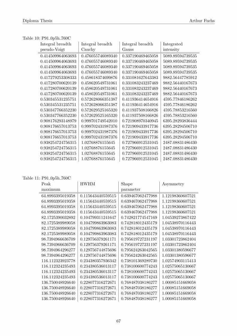
Diploma Thesis Arthur Fuchs
Table 10: P91 0p5h 760C
Integral breadth Integral breadth Integral breadth Integratedpseudo-Voigt Cauchy Gauss intensity
0.414509964063693 0.476055746089340 0.337190469465058 5089.895947395350.414509964063693 0.476055746089340 0.337190469465058 5089.895947395350.414509964063693 0.476055746089340 0.337190469465058 5089.895947395350.414509964063693 0.476055746089340 0.337190469465058 5089.895947395350.417279253308333 0.458618374699876 0.331081627643383 9882.564477859120.417280700620139 0.458620549731061 0.331083243237469 9882.564401676730.417280700620139 0.458620549731061 0.331083243237469 9882.564401676730.417280700620139 0.458620549731061 0.331083243237469 9882.564401676730.530345531235751 0.572628066351387 0.411936414654916 4595.778461862620.530345531235751 0.572628066351387 0.411936414654916 4595.778461862620.530347766352230 0.572629525165320 0.411937508166826 4595.788532165600.530347766352230 0.572629525165320 0.411937508166826 4595.788532165600.908176293148979 0.999701749542010 0.721908970340945 6395.282938364440.908176657013753 0.999702431987376 0.721909433917736 6395.282945067100.908176657013753 0.999702431987376 0.721909433917736 6395.282945067100.908176657013753 0.999702431987376 0.721909433917736 6395.282945067100.938254724756315 1.02768876155645 0.727966912531045 2487.088314864300.938254724756315 1.02768876155645 0.727966912531045 2487.088314864300.938254724756315 1.02768876155645 0.727966912531045 2487.088314864300.938254724756315 1.02768876155645 0.727966912531045 2487.08831486430
Table 11: P91 0p5h 760C
Peak HWHM Shape Asymmetrymaximum parameter
64.8993395019358 0.115643440559515 0.639467062477988 1.1219836060752164.8993395019358 0.115643440559515 0.639467062477988 1.1219836060752164.8993395019358 0.115643440559515 0.639467062477988 1.1219836060752164.8993395019358 0.115643440559515 0.639467062477988 1.1219836060752182.1725390032892 0.104799311241647 0.742821774547169 1.0453927386742282.1725389989058 0.104799863963083 0.742818012435179 1.0453897011644382.1725389989058 0.104799863963083 0.742818012435179 1.0453897011644382.1725389989058 0.104799863963083 0.742818012435179 1.0453897011644398.7394966636709 0.129756379261171 0.795619727231197 1.0330172386240498.7394966636709 0.129756379261171 0.795619727231197 1.0330172386240498.7394964296277 0.129756744875696 0.795624263042565 1.0330138059667798.7394964296277 0.129756744875696 0.795624263042565 1.03301380596677116.112323923778 0.234380357936342 0.738101369289730 1.02574903115413116.112324235493 0.234380536013117 0.738100600774243 1.02575065130667116.112324235493 0.234380536013117 0.738100600774243 1.02575065130667116.112324235493 0.234380536013117 0.738100600774243 1.02575065130667136.750048926640 0.228077316272671 0.768487038186277 1.00085151669058136.750048926640 0.228077316272671 0.768487038186277 1.00085151669058136.750048926640 0.228077316272671 0.768487038186277 1.00085151669058136.750048926640 0.228077316272671 0.768487038186277 1.00085151669058
67

Diploma Thesis Arthur Fuchs
Table 12: P91 1p5h 760C
Integral breadth Integral breadth Integral breadth Integratedpseudo-Voigt Cauchy Gauss intensity
0.366177261402393 0.414795953977922 0.297613320665316 5577.430578648360.366177261402393 0.414795953977922 0.297613320665316 5577.430578648360.366177261402393 0.414795953977922 0.297613320665316 5577.430578648360.366177261402393 0.414795953977922 0.297613320665316 5577.430578648360.379646949555851 0.408994791343633 0.293367629868689 10351.22737109400.379646949555851 0.408994791343633 0.293367629868689 10351.22737109400.379646654639386 0.408995508640324 0.293368192842500 10351.21857432900.379646891022587 0.408997226710955 0.293369515377593 10351.20858119200.464531687968059 0.492067573836691 0.350140861232518 4581.782711361020.464531881740614 0.492067641348398 0.350140906556368 4581.783878060170.464532174143415 0.492068491144420 0.350141551060399 4581.782368238770.464532174143415 0.492068491144420 0.350141551060399 4581.782368238770.770785959681230 0.845451279326925 0.610832425359612 6643.448326689660.770788976793776 0.845455831494055 0.610835800443739 6643.449467201840.770788126990665 0.845454672219675 0.610834938292847 6643.448520359730.770790966061206 0.845457961270153 0.610837349271493 6643.452421887890.836105572435249 0.865437631666447 0.606746763424706 2592.945576188290.836105572435249 0.865437631666447 0.606746763424706 2592.945576188290.836105572435249 0.865437631666447 0.606746763424706 2592.945576188290.836105572435249 0.865437631666447 0.606746763424706 2592.94557618829
Table 13: P91 1p5h 760C
Peak HWHM Shape Asymmetrymaximum parameter
64.8833797848310 0.0984230268271856 0.662789556821009 1.1528588564150064.8833797848310 0.0984230268271856 0.662789556821009 1.1528588564150064.8833797848310 0.0984230268271856 0.662789556821009 1.1528588564150064.8833797848310 0.0984230268271856 0.662789556821009 1.1528588564150082.1611315021426 0.0920186157537140 0.803867943373483 1.0818059498232282.1611315021426 0.0920186157537140 0.803867943373483 1.0818059498232282.1611315710677 0.0920187918095511 0.803860911761203 1.0818082622445882.1611316833972 0.0920192141962710 0.803850918461782 1.0818101902861898.7272618556633 0.109686661220961 0.853761285632002 1.0530782163640498.7272618506488 0.109686676808984 0.853762021116452 1.0530776688335398.7272618111474 0.109686884543075 0.853759095290150 1.0530766431831598.7272618111474 0.109686884543075 0.853759095290150 1.05307664318315116.086568355190 0.193511118250455 0.747800449897778 1.09423242308583116.086568413151 0.193512299051580 0.747796123886198 1.09423096007994116.086568386431 0.193511997746486 0.747796927713354 1.09423090862784116.086568282595 0.193512845967704 0.747796285182399 1.09422523110658136.731912583747 0.189816558014181 0.917717438072142 1.05330637473692136.731912583747 0.189816558014181 0.917717438072142 1.05330637473692136.731912583747 0.189816558014181 0.917717438072142 1.05330637473692136.731912583747 0.189816558014181 0.917717438072142 1.05330637473692
68

Diploma Thesis Arthur Fuchs
Table 14: P91 12h 760C
Integral breadth Integral breadth Integral breadth Integratedpseudo-Voigt Cauchy Gauss intensity
0.333548421020954 0.384901033130752 0.277566062080759 6200.476827677270.333548421020954 0.384901033130752 0.277566062080759 6200.476827677270.333547782671893 0.384899598044171 0.277565108034469 6200.476824276970.333547782671893 0.384899598044171 0.277565108034469 6200.476824276970.349288909262619 0.386681703261704 0.276383278901306 11737.28521195100.349286432446009 0.386676787421091 0.276379514487305 11737.29661946420.349286432446009 0.386676787421091 0.276379514487305 11737.29661946420.349286432446009 0.386676787421091 0.276379514487305 11737.29661946420.416341918816186 0.445192173386239 0.314569608900544 3695.571578966480.416341918816186 0.445192173386239 0.314569608900544 3695.571578966480.416341918816186 0.445192173386239 0.314569608900544 3695.571578966480.416341918816186 0.445192173386239 0.314569608900544 3695.571578966480.683743329439318 0.764123038774808 0.549638620158321 6900.684866189530.683743329439318 0.764123038774808 0.549638620158321 6900.684866189530.683743329439318 0.764123038774808 0.549638620158321 6900.684866189530.683743329439318 0.764123038774808 0.549638620158321 6900.684866189530.755124165093155 0.783143790457269 0.546262396160159 2864.444233450550.755119489001784 0.783135278365550 0.546256150507176 2864.443470930610.755119489001784 0.783135278365550 0.546256150507176 2864.443470930610.755119489001784 0.783135278365550 0.546256150507176 2864.44347093061
Table 15: P91 12h 760C
Peak HWHM Shape Asymmetrymaximum parameter
64.9245282900980 0.0897420400351990 0.601866455106988 1.1836772499758764.9245282900980 0.0897420400351990 0.601866455106988 1.1836772499758764.9245279525372 0.0897417033959266 0.601871454378399 1.1836706474997964.9245279525372 0.0897417033959266 0.601871454378399 1.1836706474997982.2143763265198 0.0863697079908372 0.731746388673641 1.1179634068987582.2143765227169 0.0863684597019364 0.731762837293301 1.1179702138482682.2143765227169 0.0863684597019364 0.731762837293301 1.1179702138482682.2143765227169 0.0863684597019364 0.731762837293301 1.1179702138482698.7736801548981 0.0983140428206316 0.833122391738689 1.0581006920249198.7736801548981 0.0983140428206316 0.833122391738689 1.0581006920249198.7736801548981 0.0983140428206316 0.833122391738689 1.0581006920249198.7736801548981 0.0983140428206316 0.833122391738689 1.05810069202491116.126483214169 0.172524798199945 0.698744613002953 1.12388631033446116.126483214169 0.172524798199945 0.698744613002953 1.12388631033446116.126483214169 0.172524798199945 0.698744613002953 1.12388631033446116.126483214169 0.172524798199945 0.698744613002953 1.12388631033446136.774341862071 0.170691267907944 0.914431422867559 1.09631184153677136.774342959736 0.170689298086170 0.914442767358552 1.09631605089046136.774342959736 0.170689298086170 0.914442767358552 1.09631605089046136.774342959736 0.170689298086170 0.914442767358552 1.09631605089046
69

Diploma Thesis Arthur Fuchs
Table 16: P91 24h 760C
Integral breadth Integral breadth Integral breadth Integratedpseudo-Voigt Cauchy Gauss intensity
0.305692509958350 0.346288860439689 0.250317257621689 5912.248640566800.305694016484607 0.346292444627294 0.250319862293378 5912.242058924350.305694016484607 0.346292444627294 0.250319862293378 5912.242058924350.305694016484607 0.346292444627294 0.250319862293378 5912.242058924350.323848006168151 0.352227226350850 0.249862598258243 10802.29338706540.323847497000257 0.352222720724925 0.249859116341985 10802.32356235120.323847497000257 0.352222720724925 0.249859116341985 10802.32356235120.323847497000257 0.352222720724925 0.249859116341985 10802.32356235120.390192721324623 0.417695456038596 0.293686726170199 3800.965515274860.390192668070817 0.417689718116537 0.293682447936976 3800.987019264150.390192668070817 0.417689718116537 0.293682447936976 3800.987019264150.390192668070817 0.417689718116537 0.293682447936976 3800.987019264150.613532669250457 0.676673954332981 0.482080263578520 7110.867432319290.613533313748809 0.676673287814297 0.482079652208242 7110.874358563770.613536798373287 0.676679310256803 0.482084200209241 7110.871489518620.613536798373287 0.676679310256803 0.482084200209241 7110.871489518620.695418230651589 0.712274325462526 0.494122933816402 2802.869677037490.695418230651589 0.712274325462526 0.494122933816402 2802.869677037490.695430585048691 0.712316451752918 0.494153179261912 2802.843033721790.695430585048691 0.712316451752918 0.494153179261912 2802.84303372179
Table 17: P91 24h 760C
Peak HWHM Shape Asymmetrymaximum parameter
64.9367094057584 0.0794152054440875 0.653622048349723 1.1468349403979464.9367096818125 0.0794161161170344 0.653605959358552 1.1468373146903364.9367096818125 0.0794161161170344 0.653605959358552 1.1468373146903364.9367096818125 0.0794161161170344 0.653605959358552 1.1468373146903382.2133188521652 0.0780424344617268 0.786100106256457 1.0994628461586682.2133189070837 0.0780413370341047 0.786130733633185 1.0994608373118882.2133189070837 0.0780413370341047 0.786130733633185 1.0994608373118882.2133189070837 0.0780413370341047 0.786130733633185 1.0994608373118898.7751517679573 0.0918418068009864 0.833072159664589 1.0519341217324698.7751520111362 0.0918404664441726 0.833107106698686 1.0519384954337398.7751520111362 0.0918404664441726 0.833107106698686 1.0519384954337398.7751520111362 0.0918404664441726 0.833107106698686 1.05193849543373116.136778683636 0.150900456514930 0.745043363951511 1.08698163250808116.136778695893 0.150900288045291 0.745049176566665 1.08697596043069116.136778315545 0.150901778368869 0.745039903781976 1.08696845150169116.136778315545 0.150901778368869 0.745039903781976 1.08696845150169136.771319937993 0.154461112829177 0.945098031378775 1.07171325190312136.771319937993 0.154461112829177 0.945098031378775 1.07171325190312136.771315650699 0.154470534146649 0.945001667283013 1.07168923566038136.771315650699 0.154470534146649 0.945001667283013 1.07168923566038
70
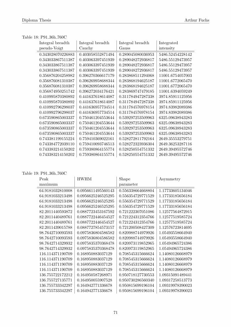
Diploma Thesis Arthur Fuchs
Table 18: P91 36h 760C
Integral breadth Integral breadth Integral breadth Integratedpseudo-Voigt Cauchy Gauss intensity
0.343028070226883 0.403058552871494 0.289045080036953 5486.524542281420.343033867511387 0.403063397451939 0.289048272936817 5486.551294739570.343033867511387 0.403063397451939 0.289048272936817 5486.551294739570.343033867511387 0.403063397451939 0.289048272936817 5486.551294739570.356876204258982 0.396270366617179 0.283868511294068 11001.67540570030.356876081310387 0.396269958688344 0.283868194625187 11001.67720654700.356876081310387 0.396269958688344 0.283868194625187 11001.67720654700.356874950251742 0.396272034176421 0.283869747479185 11001.63940592490.410995870380892 0.441637618614087 0.311784947287338 3974.859111259560.410995870380892 0.441637618614087 0.311784947287338 3974.859111259560.410992796298037 0.441636957734514 0.311784576978154 3974.839820893860.410992796298037 0.441636957734514 0.311784576978154 3974.839820893860.673590865003337 0.750461204553644 0.539297253509963 6325.096389432830.673590865003337 0.750461204553644 0.539297253509963 6325.096389432830.673590865003337 0.750461204553644 0.539297253509963 6325.096389432830.673590865003337 0.750461204553644 0.539297253509963 6325.096389432830.743381199155224 0.759410369022161 0.528272811792164 2649.355532797510.743384772039110 0.759410093746513 0.528272323936304 2649.362532871160.743383214150202 0.759380864155774 0.528250554751332 2649.394955727460.743383214150202 0.759380864155774 0.528250554751332 2649.39495572746
Table 19: P91 36h 760C
Peak HWHM Shape Asymmetrymaximum parameter
64.9181032810008 0.0956611495560143 0.556338664668804 1.1773360513404664.9181033213498 0.0956625246525295 0.556354729771529 1.1773318565618464.9181033213498 0.0956625246525295 0.556354729771529 1.1773318565618464.9181033213498 0.0956625246525295 0.556354729771529 1.1773318565618482.2011440593872 0.0887723453167592 0.721222307051086 1.1257756487291582.2011440489761 0.0887722446454527 0.721224312354766 1.1257751958572482.2011440489761 0.0887722446454527 0.721224312354766 1.1257751958572482.2011439015788 0.0887727854573157 0.721200508427309 1.1257672381469598.7642710093593 0.0975836804586582 0.820988744979926 1.0549355866494098.7642710093593 0.0975836804586582 0.820988744979926 1.0549355866494098.7642714329932 0.0975835370368478 0.820973119852965 1.0549496572438698.7642714329932 0.0975835370368478 0.820973119852965 1.05494965724386116.114371190709 0.168950883037129 0.708545315666624 1.14080126668979116.114371190709 0.168950883037129 0.708545315666624 1.14080126668979116.114371190709 0.168950883037129 0.708545315666624 1.14080126668979116.114371190709 0.168950883037129 0.708545315666624 1.14080126668979136.755722172212 0.164950587268971 0.950718127730553 1.09315091489441136.755727135771 0.164950055907528 0.950730286560340 1.09317258513773136.755733342297 0.164942771336678 0.950815699196104 1.09319978390023136.755733342297 0.164942771336678 0.950815699196104 1.09319978390023
71

Diploma Thesis Arthur Fuchs
9.5 Determination of q
The following figures (69 to 75) show the plots to determine the parameter q to then calculate thecontrast factor C.
Figure 69: Determination of the parameter q for sample P91 BH vib pol
Figure 70: Determination of the parameter q forsample P91 0p166h 760C
Figure 71: Determination of the parameter q forsample P91 0p5h 760C
72

Diploma Thesis Arthur Fuchs
Figure 72: Determination of the parameter q forsample P91 1p5h 760C
Figure 73: Determination of the parameter q forsample P91 12h 760C
Figure 74: Determination of the parameter q forsample P91 24h 760C
Figure 75: Determination of the parameter q forsample P91 36h 760C
9.6 Matlab codes
9.6.1 Peak fitting
To run the programs please also download the routines ”pseudoVoigtAsym”, ”pseudoVoigtAsymDeriv”and ”pseudoVoigtAsymFit” from http://www.xray.cz/xrdmlread/Add-ons.htm. Also the files ”pseu-doVoigtAsym C G separate” and ”pseudoVoigtAsym separate” are needed (see below). These twofiles are mostly identical to ”pseudoVoigtAsym” but have been adapted by the author of this work.
9.6.2 pseudoVoigtAsym C G separate
The Matlab code for ”pseudoVoigtAsym C G separate” is:
73

Diploma Thesis Arthur Fuchs
function [y,y_c,y_g] = pseudoVoigtAsym(a,x)
%--------------------------------------------------------------
%%%%----This file was downloaded from
%%%%http://www.xray.cz/xrdmlread/Add-ons.htm
%%%%and the author only adapted minor changes!!!----
%-------------------------------------------------------------
% PSEUDOVOIGTASYM Calculate values of the asymmetric
% pseudo-Voigt function.
%
% [y] = pseudoVoigtAsym(a,x)
%
% a - parameters of the asymmetric pseudo-Voigt function
% x - a (row) vector of points where the asymmetric
% pseudo-Voigt should be calculated.
%
% y - calculated values of the asym. pseudo-Voigt function
%
% example: a Gauss-like peak
%
% x = [-10:0.1:10];
% a = [1.0, 2.0, 1.5, 0.0, 1.0];
% y = pseudoVoigtAsym(a,x);
% plot(x,y)
%
% The integral of the asym. pseudo-Voigt function is normalized
% to one and hence the function is defined as:
%
% y = a1 * { (1-a4) * sqrt[log(2)/pi/ss^2]
% * exp[-log(2)/s^2*(x-a2)^2]
% + a4 * 1/pi/ss * 1 / [ 1 + (x-a2)^2/s^2) ] },
%
% where ss and s are defined as follows:
%
% ss = 1/4*(2 + a5 + 1/a5)*a3
%
% s = 1/2*(1 + a5)*a3 for x < a2,
% s = 1/2*(1 + 1/a5)*a3 for x >= a2.
%
% Parameters have this meaning:
%
% a1 - integrated intensity
% a2 - maximum position
% a3 - HWHM - half width in the half of maximum
% (for symmetrical profiles)
% a4 - Cauchy/Gauss component weight (0 - Gauss, 1 - Cauchy)
% a5 - asymmetry (1 - symmetric)
%
% FWHM = 1/2*(2+a5+1/a5)*a3
%
% Function parametes (a) should be optionally stored in
74

Diploma Thesis Arthur Fuchs
% a vector of the size (1 x 5). If input parameters (a)
% represent a matrix of size (n x 5), n pseudo-Voigt
% functions are returned in n rows of the output vector y.
%
% X-ray diffraction: global WAVELENGTHS
%
% Function support a global variable WAVELENGTHS that
% represent an array of size (m x 2), where m is a number
% of spectral lines. (In scripts if for example sigle peaks
% are generated take caution that these variables were not
% previosly defined by another script.) The WAVELENGTHS matrix
% has this interpretation:
%
% the 1st column - relative line intensity
% the 2st column - delta(Lambda)/Lambda ratio
% (Lambda is an averaged wavelength)
%
% example: CuKalpha1 + CuKalpha1 (Lambda = 1.5419)
%
% WAVELENGTHS =
% 1.0000 -0.0008
% 0.5000 0.0017
%
% Ref.: The function has been adapted from
% [1] H. Toraya, J.Appl.Cryst 23 (1990), 485-491
% [2] ObjCryst/FOX - V. Favre-Nicolin, J.Appl.Cryst. 35 (2002), 734-743
%
% See also pseudoVoigtAsymDeriv, pseudVoigtAsymFit
%
% version 1.1, 19.11.2013, (c) Zdenek Matej
%--------------------------------------------------------------
global WAVELENGTH_SEPARATE
global normierung
% check parameters
if ~exist(’WAVELENGTH_SEPARATE’,’var’) | isempty(WAVELENGTH_SEPARATE)
WAVELENGTH_SEPARATE=[1.0 0.0];
end
if size(x,1)>1 x = reshape(x,1,[]); end
if size(a,2)~=5 a = reshape(a,[],5); end
% calc. all sets (sum over all spectral lines)
y = zeros(size(a,1),length(x));
y_c = zeros(size(a,1),length(x));
y_g = zeros(size(a,1),length(x));
for j=1:size(a,1)
for k=1:size(WAVELENGTH_SEPARATE,1)
a2 = a(j,2)+tan(a(j,2)*pi/360)*WAVELENGTH_SEPARATE(k,2)*360/pi;
Lind = x < a(j,2);
s1 = (1. + a(j,5))*a(j,3)/2;
s2 = (1. + 1./a(j,5))*a(j,3)/2;
ss = (s1 + s2)/2;
75

Diploma Thesis Arthur Fuchs
c = (1-a(j,4))*sqrt(log(2)/pi/ss^2);
y_g(j, Lind) = y_g(j, Lind) + WAVELENGTH_SEPARATE(k,1)*c*...
exp(-log(2)/s1^2*(x( Lind)-a2).^2);
y_g(j,~Lind) = y_g(j,~Lind) + WAVELENGTH_SEPARATE(k,1)*c*...
exp(-log(2)/s2^2*(x(~Lind)-a2).^2);
c = a(j,4)/pi/ss;
y_c(j, Lind) = y_c(j, Lind) + WAVELENGTH_SEPARATE(k,1)*...
c./(1+(x( Lind)-a2).^2/s1^2);
y_c(j,~Lind) = y_c(j,~Lind) + WAVELENGTH_SEPARATE(k,1)*...
c./(1+(x(~Lind)-a2).^2/s2^2);
y(j,:) = y_c(j,:) + y_g(j,:);
end
y_c(j,:) = a(j,1)*y_c(j,:)/normierung;
y_g(j,:) = a(j,1)*y_g(j,:)/normierung;
y(j,:) = a(j,1)*y(j,:)/normierung;
end
return;
9.6.3 pseudoVoigtAsym separate
The Matlab code for ”pseudoVoigtAsym separate” is:
function [y] = pseudoVoigtAsym(a,x)
%--------------------------------------------------------------
%%%%----This file was downloaded from
%%%%http://www.xray.cz/xrdmlread/Add-ons.htm
%%%%and the author only adapted minor changes!!!----
%-------------------------------------------------------------
% PSEUDOVOIGTASYM Calculate values of the asymmetric
% pseudo-Voigt function.
%
% [y] = pseudoVoigtAsym(a,x)
%
% a - parameters of the asymmetric pseudo-Voigt function
% x - a (row) vector of points where the asymmetric
% pseudo-Voigt should be calculated.
%
% y - calculated values of the asym. pseudo-Voigt function
%
% example: a Gauss-like peak
%
% x = [-10:0.1:10];
% a = [1.0, 2.0, 1.5, 0.0, 1.0];
% y = pseudoVoigtAsym(a,x);
% plot(x,y)
%
% The integral of the asym. pseudo-Voigt function is normalized
% to one and hence the function is defined as:
%
76

Diploma Thesis Arthur Fuchs
% y = a1 * { (1-a4) * sqrt[log(2)/pi/ss^2]
% * exp[-log(2)/s^2*(x-a2)^2]
% + a4 * 1/pi/ss * 1 / [ 1 + (x-a2)^2/s^2) ] },
%
% where ss and s are defined as follows:
%
% ss = 1/4*(2 + a5 + 1/a5)*a3
%
% s = 1/2*(1 + a5)*a3 for x < a2,
% s = 1/2*(1 + 1/a5)*a3 for x >= a2.
%
% Parameters have this meaning:
%
% a1 - integrated intensity
% a2 - maximum position
% a3 - HWHM - half width in the half of maximum
% (for symmetrical profiles)
% a4 - Cauchy/Gauss component weight (0 - Gauss, 1 - Cauchy)
% a5 - asymmetry (1 - symmetric)
%
% FWHM = 1/2*(2+a5+1/a5)*a3
%
% Function parametes (a) should be optionally stored in
% a vector of the size (1 x 5). If input parameters (a)
% represent a matrix of size (n x 5), n pseudo-Voigt
% functions are returned in n rows of the output vector y.
%
% X-ray diffraction: global WAVELENGTHS
%
% Function support a global variable WAVELENGTHS that
% represent an array of size (m x 2), where m is a number
% of spectral lines. (In scripts if for example sigle peaks
% are generated take caution that these variables were not
% previosly defined by another script.) The WAVELENGTHS matrix
% has this interpretation:
%
% the 1st column - relative line intensity
% the 2st column - delta(Lambda)/Lambda ratio
% (Lambda is an averaged wavelength)
%
% example: CuKalpha1 + CuKalpha1 (Lambda = 1.5419)
%
% WAVELENGTHS =
% 1.0000 -0.0008
% 0.5000 0.0017
%
% Ref.: The function has been adapted from
% [1] H. Toraya, J.Appl.Cryst 23 (1990), 485-491
% [2] ObjCryst/FOX - V. Favre-Nicolin, J.Appl.Cryst. 35 (2002), 734-743
%
77

Diploma Thesis Arthur Fuchs
% See also pseudoVoigtAsymDeriv, pseudVoigtAsymFit
%
% version 1.1, 19.11.2013, (c) Zdenek Matej
%--------------------------------------------------------------
global WAVELENGTH_SEPARATE
global normierung
% check parameters
if ~exist(’WAVELENGTH_SEPARATE’,’var’) | isempty(WAVELENGTH_SEPARATE)
WAVELENGTH_SEPARATE=[1.0 0.0];
end
if size(x,1)>1 x = reshape(x,1,[]); end
if size(a,2)~=5 a = reshape(a,[],5); end
% calc. all sets (sum over all spectral lines)
y = zeros(size(a,1),length(x));
for j=1:size(a,1)
for k=1:size(WAVELENGTH_SEPARATE,1)
a2 = a(j,2)+tan(a(j,2)*pi/360)*WAVELENGTH_SEPARATE(k,2)*360/pi;
Lind = x < a(j,2);
s1 = (1. + a(j,5))*a(j,3)/2;
s2 = (1. + 1./a(j,5))*a(j,3)/2;
ss = (s1 + s2)/2;
c = (1-a(j,4))*sqrt(log(2)/pi/ss^2);
y(j, Lind) = y(j, Lind) + WAVELENGTH_SEPARATE(k,1)*c*...
exp(-log(2)/s1^2*(x( Lind)-a2).^2);
y(j,~Lind) = y(j,~Lind) + WAVELENGTH_SEPARATE(k,1)*c*...
exp(-log(2)/s2^2*(x(~Lind)-a2).^2);
c = a(j,4)/pi/ss;
y(j, Lind) = y(j, Lind) + WAVELENGTH_SEPARATE(k,1)*...
c./(1+(x( Lind)-a2).^2/s1^2);
y(j,~Lind) = y(j,~Lind) + WAVELENGTH_SEPARATE(k,1)*...
c./(1+(x(~Lind)-a2).^2/s2^2);
end
y(j,:) = a(j,1)*y(j,:)/normierung;
%y(j,:) = a(j,1)*y(j,:)/sum(WAVELENGTH_SEPARATE(:,1));
end
return;
9.6.4 LaB6 peak fit
The Matlab code for the LaB6 peak fitting routine is:
close all
clear all
clc
%------------Specify x-ray radiation-----------------
Cu_K_alpha1 = 1.540598*10^-10; % Cu_K_alpha1 wavelength
Cu_K_alpha2 = 1.544426*10^-10; % Cu_K_alpha2 wavelength
intensity_Kalpha1 = 1; % Cu_K_alpha1 intensity
intensity_Kalpha2 = 0.5; % Cu_K_alpha2 intensity
78

Diploma Thesis Arthur Fuchs
global WAVELENGTH_SEPARATE; % For separate K_alpha1/K_alpha2 calculations
global normierung % For Scaling area under peaks with intensity
normierung = intensity_Kalpha1 + intensity_Kalpha2;
global WAVELENGTHS %For combined K_alpha1/K_alpha2 calculations
Cu_K_alpha = (intensity_Kalpha1*Cu_K_alpha1 + intensity_Kalpha2...
* Cu_K_alpha2) / normierung;
delta_Cu_K_alpha1 = (Cu_K_alpha1 - Cu_K_alpha);
delta_Cu_K_alpha2 = (Cu_K_alpha2 - Cu_K_alpha);
WAVELENGTHS = [intensity_Kalpha1 delta_Cu_K_alpha1/Cu_K_alpha;...
intensity_Kalpha2 delta_Cu_K_alpha2/Cu_K_alpha];
% Import data: When measuring the whole data at once, use the M=... ,
% otherwise import the data with M_xx=... in separate files.
%M = load(’LaB6_standard_parallel_beam_20h.xy’,’-ascii’);
M_21 = load(’LaB6_18-24_SLD_mono.xy’,’-ascii’);
M_36_58 = load(’LaB6_36-58_SLD_mono.xy’,’-ascii’);
M_74_81 = load(’LaB6_74-81_SLD_mono.xy’,’-ascii’);
M_82_142 = load(’LaB6_82-142_SLD_mono.xy’,’-ascii’);
%peaknamen = [21 30 37 43 49 54 76 80 84 88 96 100 104 108 112 121 ...
% 131 136 142]; % If all peaks can be analysed
peaknamen = [21 37 43 49 54 76 80 84 88 96 100 104 108 112 116 121 131 ...
136 142]; % If the 30° peaks is too small to be analysed. Often
% happens when measuring with the physics department’s PANalytical
% x-ray-machine with monochromator.
% %Define evaluation range: Use this if all data was importet in one file:
% x_data_LaB6_21 = M(610:1050,1).’;
% y_data_LaB6_21 = M(610:1050,2).’;
% x_data_LaB6_30 = M(1350:1715,1).’;
% y_data_LaB6_30 = M(1350:1715,2).’;
% x_data_LaB6_37 = M(1905:2290,1).’;
% y_data_LaB6_37 = M(1905:2290,2).’;
% x_data_LaB6_43 = M(2360:2745,1).’;
% y_data_LaB6_43 = M(2360:2745,2).’;
% x_data_LaB6_49 = M(2820:3125,1).’;
% y_data_LaB6_49 = M(2820:3125,2).’;
% x_data_LaB6_54 = M(3200:3505,1).’;
% y_data_LaB6_54 = M(3200:3505,2).’;
% x_data_LaB6_76 = M(4875:5180,1).’;
% y_data_LaB6_76 = M(4875:5180,2).’;
% x_data_LaB6_80 = M(5180:5485,1).’;
% y_data_LaB6_80 = M(5180:5485,2).’;
% x_data_LaB6_84 = M(5485:5790,1).’;
79

Diploma Thesis Arthur Fuchs
% y_data_LaB6_84 = M(5485:5790,2).’;
% x_data_LaB6_88 = M(5790:6095,1).’;
% y_data_LaB6_88 = M(5790:6095,2).’;
% x_data_LaB6_96 = M(6400:6705,1).’;
% y_data_LaB6_96 = M(6400:6705,2).’;
% x_data_LaB6_100 = M(6705:7010,1).’;
% y_data_LaB6_100 = M(6705:7010,2).’;
% x_data_LaB6_104 = M(7010:7315,1).’;
% y_data_LaB6_104 = M(7010:7315,2).’;
% x_data_LaB6_108 = M(7315:7620,1).’;
% y_data_LaB6_108 = M(7315:7620,2).’;
% x_data_LaB6_112 = M(7620:7925,1).’;
% y_data_LaB6_112 = M(7620:7925,2).’;
% x_data_LaB6_121 = M(8300:8610,1).’;
% y_data_LaB6_121 = M(8300:8610,2).’;
% x_data_LaB6_131 = M(9065:9300,1).’;
% y_data_LaB6_131 = M(9065:9300,2).’;
% x_data_LaB6_136 = M(9445:9750,1).’;
% y_data_LaB6_136 = M(9445:9750,2).’;
% x_data_LaB6_142 = M(9830:10285,1).’;
% y_data_LaB6_142 = M(9830:10285,2).’;
%Define evaluation range: Use this if data was importet in separated files:
x_data_LaB6_21 = M_21(210:end,1).’;
y_data_LaB6_21 = M_21(210:end,2).’;
x_data_LaB6_37 = M_36_58(55:245,1).’;
y_data_LaB6_37 = M_36_58(55:245,2).’;
x_data_LaB6_43 = M_36_58(510:702,1).’;
y_data_LaB6_43 = M_36_58(510:702,2).’;
x_data_LaB6_49 = M_36_58(892:1160,1).’;
y_data_LaB6_49 = M_36_58(892:1160,2).’;
x_data_LaB6_54 = M_36_58(1273:1578,1).’;
y_data_LaB6_54 = M_36_58(1273:1578,2).’;
x_data_LaB6_76 = M_74_81(1:215,1).’;
y_data_LaB6_76 = M_74_81(1:215,2).’;
x_data_LaB6_80 = M_74_81(344:496,1).’;
y_data_LaB6_80 = M_74_81(344:496,2).’;
x_data_LaB6_84 = M_82_142(39:191,1).’;
y_data_LaB6_84 = M_82_142(39:191,2).’;
x_data_LaB6_88 = M_82_142(306:534,1).’;
y_data_LaB6_88 = M_82_142(306:534,2).’;
x_data_LaB6_96 = M_82_142(953:1105,1).’;
y_data_LaB6_96 = M_82_142(953:1105,2).’;
x_data_LaB6_100 = M_82_142(1182:1448,1).’;
y_data_LaB6_100 = M_82_142(1182:1448,2).’;
x_data_LaB6_104 = M_82_142(1486:1791,1).’;
y_data_LaB6_104 = M_82_142(1486:1791,2).’;
x_data_LaB6_108 = M_82_142(1829:2057,1).’;
y_data_LaB6_108 = M_82_142(1829:2057,2).’;
x_data_LaB6_112 = M_82_142(2134:2362,1).’;
80

Diploma Thesis Arthur Fuchs
y_data_LaB6_112 = M_82_142(2134:2362,2).’;
x_data_LaB6_116 = M_82_142(2438:2743,1).’;
y_data_LaB6_116 = M_82_142(2438:2743,2).’;
x_data_LaB6_121 = M_82_142(2819:3047,1).’;
y_data_LaB6_121 = M_82_142(2819:3047,2).’;
x_data_LaB6_131 = M_82_142(3543:3809,1).’;
y_data_LaB6_131 = M_82_142(3543:3809,2).’;
x_data_LaB6_136 = M_82_142(3961:4190,1).’;
y_data_LaB6_136 = M_82_142(3961:4190,2).’;
x_data_LaB6_142 = M_82_142(4380:end,1).’;
y_data_LaB6_142 = M_82_142(4380:end,2).’;
% Give approximate positions of peak maxima in 2Theta:
peakmax_data_21 = 21.4;
%peakmax_data_30 = 30.4;
peakmax_data_37 = 37.4;
peakmax_data_43 = 43.5;
peakmax_data_49 = 49.0;
peakmax_data_54 = 54.0;
peakmax_data_76 = 75.9;
peakmax_data_80 = 79.9;
peakmax_data_84 = 83.9;
peakmax_data_88 = 87.8;
peakmax_data_96 = 95.7;
peakmax_data_100 = 99.7;
peakmax_data_104 = 103.7;
peakmax_data_108 = 107.8;
peakmax_data_112 = 112.0;
peakmax_data_116 = 116.4;
peakmax_data_121 = 120.9;
peakmax_data_131 = 130.6;
peakmax_data_136 = 136.0;
peakmax_data_142 = 142.0;
fitting_iterations = 3000; % Define how many sets of starting parameters
% for "Monte-Carlo-method" should be given.
%------------------------Begin of peak evaluation------------------------
%!!!!Important:!!!!
% a(1) - integrated intensity
% a(2) - maximum position
% a(3) - HWHM - half width in the half of maximum
% (for symmetrical profiles)
% a(4) - Cauchy/Gauss component weight (0 - Gauss, 1 - Cauchy)
% a(5) - asymmetry (1 - symmetric)
% For-loop over all peaks:
for ges = 1 : numel(peaknamen)
% Get the right peak maximum for the peak:
81

Diploma Thesis Arthur Fuchs
peakmax_data = eval([’peakmax_data_’ int2str(peaknamen(ges))]);
% Get right data range for the peak:
x_data = eval([’x_data_LaB6_’ int2str(peaknamen(ges))]);
y_data = eval([’y_data_LaB6_’ int2str(peaknamen(ges))]);
% Estimate starting parameters:
background = 1000; % Variable for background estimation in counts
x = 0.5; % Chauchy/Gauss (see a(4))
II_max = 120000; % Estimated maximum of integrated intensity in counts
HWHM_max = 0.1; % Estimatet Half-Width-at-Half-Maximum in 2Theta
HWHM_var = 0.1; % Variation around the estimated HWHM in 2Theta
peakvar = 0.3; % Variation of the estimated peak maxima
mu(1) = (x_data(1)+x_data(end))/2; %(see function: pseudoVoigtAsym.m)
mu(2) = x_data(end)-x_data(1); %(see function: pseudoVoigtAsym.m)
Linda = [1 1 1 1 1]; % Determine which parts of a(1-5) should be fitted:
% 1-Perform fit, 0-do not fit
b0 = [0 0 background]; % Guess background function y=b0(1)x^2+b0(2)x+b0(3)
Lindb = [1 1 1]; % Determine which parts of background b(1-3) should
% be fitted: 1-Perform fit, 0-do not fit
w = 1./y_data; %(see function: pseudoVoigtAsym.m)
% Define variables to be filled later:
rwp_final = 1000;
a_final = [0,0,0,0,0];
b_final = NaN;
a0_final = [0,0,0,0,0];
counter = 1;
a_final_faul = zeros(4,5);
IB_ges_faul = zeros(4,1);
IB_cauchy_faul = zeros(4,1);
IB_gauss_faul = zeros(4,1);
b_final_faul = zeros(4,3);
% For-loop to do each data processing 4 times to get a feeling of the fit
% stability:
for faul = 1:4
% Perform fitting with "Monte-Carlo-Simulation":
for counter = 1:fitting_iterations
% Randomize starting parameters:
h = rand * II_max; % Integrated intensity
j = HWHM_max + (2*rand -1) * HWHM_var; % HWHM
i = peakmax_data + (2*rand -1) * peakvar; % Peak maximum in 2Theta
k = x + (2*rand -1) * 0.5; % Chauchy/Gauss weight
% (0 - Gauss, 1 - Cauchy)
asym = 1 + (2*rand -1) * 0.1; % Asymmetry (1 - symmetric)
82

Diploma Thesis Arthur Fuchs
a0 = [h, i, j, k, asym];
% Perform fitting:
[a_fit,b_fit,~,~,~,rwp] =...
pseudoVoigtAsymFit(x_data,y_data,w,a0,b0,mu,Linda,Lindb);
if 0<=a_fit(4) % Make sure peak shape is exact or between Gauss/Cauchy
if a_fit(4)<=1 % Make sure peak shape is exact or between Gauss/Cauchy
if rwp < rwp_final % Only save if fit is better than
a_final = a_fit; % previously best one.
b_final = b_fit;
a0_final = a0;
rwp_final = rwp;
intensity_Kalpha2_final = intensity_Kalpha2;
end
end
end
counter = counter +1
end
%---------------Define parameters for plotting:---------------
% Draw background function:
background = polyval(b_final,x_data,[],mu);
% Complete fit including Gauss & Cauchy and K_alpha1 & K_alpha2 parts:
yc_fit = sum(pseudoVoigtAsym(a_final,x_data),1)...
+background; % Convert data fit into curve
yc_schaetz = sum(pseudoVoigtAsym(a0_final,x_data),1)...
+polyval(b0,x_data,[],mu); % Convert starting parameters for best fit
% into curve
%Create curve for Gauss & Cauchy and K_alpha1 (NO K_alpha2!):
WAVELENGTH_SEPARATE = [intensity_Kalpha1 delta_Cu_K_alpha1/Cu_K_alpha];
yc_fit_Kalpha1 = sum(pseudoVoigtAsym_separate(a_final,x_data),1)...
+background;
%Also separate Gauss and Cauchy parts (of K_alpha1 peak):
[~,ycauchy1,ygauss1] = pseudoVoigtAsym_C_G_separate(a_final,x_data);
%Find maximum of K_alpha1 peak:
ind_ges1 = find(pseudoVoigtAsym_separate(a_final,x_data)>=...
max(pseudoVoigtAsym_separate(a_final,x_data)));
%Create curve for Gauss & Cauchy and K_alpha2 (NO K_alpha1!):
WAVELENGTH_SEPARATE = [intensity_Kalpha2 delta_Cu_K_alpha2/Cu_K_alpha];
yc_fit_Kalpha2 = sum(pseudoVoigtAsym_separate(a_final,x_data),1)...
+background;
%Again separate Gauss and Cauchy parts (of K_alpha2 peak):
[y,ycauchy2,ygauss2] = pseudoVoigtAsym_C_G_separate(a_final,x_data);
%Combine Cauchy_K_alpha1 and Cauchy_K_alpha2:
83

Diploma Thesis Arthur Fuchs
ycauchy = ycauchy1 + ycauchy2;
%Combine Gauss_K_alpha1 and Gauss_K_alpha2:
ygauss = ygauss1 + ygauss2;
%Combine Kalpha1 and Kalpha2 fit to make sure they give the same result as
%the combined fit:
yc_fit_Kalpha_test = yc_fit_Kalpha1 + yc_fit_Kalpha2...
-background;
%Check if Gauss/Cauchy separation worked correctly. If it works for Kalpha2
%peak, it is assumed that it also worked for Kalpha1:
if y ~= pseudoVoigtAsym_separate(a_final,x_data)
errormessage=[’Der Funktionierer ist kaputt!(Gauss+Lorentz-Kurve ’...
’~= Gesamtfit) \nThis usually happes if the fit function did ’...
’not find a minimum’];
error(errormessage,[ ])
end
% Get 2Theta angle of overall peak maximum (K_alpha1&2 together):
x1 = x_data(ind_ges1);
% Sum Cauchy parts and background for plotting:
ycauchy_plot = sum(ycauchy,1)+background;
% Find maximum position of Cauchy K_alpha1 peak:
ind_cauchy = find(ycauchy1>=max(ycauchy1));
% Sum Gauss parts and background for plotting:
ygauss_plot = sum(ygauss,1)+background;
% Find maximum position of Gauss K_alpha1 peak:
ind_gauss = find(ygauss1>=max(ygauss1));
%---Difference plot------
y_diff = y_data - yc_fit;
%!!!!!!!!!!!IMPORTANT!!!!!!!!!!!
% The plots here are done for every of of the 4 repetitions, one can
% visually analyse each peak and search for problems if something big
% goes wrong! For normal data analysis the two plots at the end should do.
% % This Plot is to compare the data with the fit, the K_alpha1 and
% % K_alpha2 peaks separately, the background function and the peak
% % maximum:
% figure
% semilogy(x_data,y_data,’k*’)
% hold on
% semilogy(x_data,yc_fit,’m’)
% semilogy(x_data,yc_fit_Kalpha1,’r’)
% semilogy(x_data,background,’y’)
% line([x1 x1], get(gca, ’ylim’),’color’,’c’,’LineStyle’,’-.’);
% semilogy(x_data,yc_fit_Kalpha2,’r’)
% xlabel (’Winkel 2 \Theta [°]’)
84

Diploma Thesis Arthur Fuchs
% ylabel (’Counts [a.u.]’)
% legend (’Messdaten’,’Gefittete Kurve’,’K_{\alpha1} und K_{\alpha2}...
% separat gefittet’,’Untergrund’,’Maximum’)
% hold off
% % The next Plot is to compare the data with the fit, the starting
% % parameters that gave the best fit results, the background function, the
% % peak maximum and to check if separation has worked properly (The fittet
% % curve should be overplottet by a curve that is the sum of all
% % previously separated K_alpha1+K_alpha2 curves).
%
% figure
% semilogy(x_data,y_data,’k*’)
% hold on
% semilogy(x_data,yc_schaetz,’g’)
% semilogy(x_data,yc_fit,’m’)
% semilogy(x_data,yc_fit_Kalpha_test,’b’)
% semilogy(x_data,background,’y’)
% line([x1 x1], get(gca, ’ylim’),’color’,’c’,’LineStyle’,’-.’);
% xlabel (’Winkel 2 \Theta [°]’)
% ylabel (’Counts [a.u.]’)
% legend (’Messdaten’,’Geschaetzte Anfangsparameter’,’Gefittete Kurve’,...
% ’K_{\alpha1} + K_{\alpha2}’,’Untergrund’,’Maximum’)
% hold off
% % The next Plot is to compare the data with the fit, the background
% % function, the peak maximum, Cauchy and Gauss peaks separately and to
% % check if separation has worked properly (The fittet curve should be
% % overplottet by a curve that is the sum of the previously separated
% % Cauchy- and Gauss-curves).
% figure
% semilogy(x_data,y_data,’k*’)
% hold on
% semilogy(x_data,yc_fit,’m’)
% %semilogy(x_data,yc_fit_Kalpha1,’r’)
% semilogy(x_data,background,’y’)
% %semilogy(x_data,yc_fit_Kalpha_test,’b’)
% line([x1 x1], get(gca, ’ylim’),’color’,’c’,’LineStyle’,’-.’);
% semilogy(x_data,ygauss_plot,’g’)
% semilogy(x_data,ycauchy_plot,’c’)
% semilogy(x_data,ygauss_plot+ycauchy,’r’)
% %semilogy(x_data,yc_fit_Kalpha2,’r’)
% xlabel (’Winkel 2 \Theta [°]’)
% ylabel (’Counts [a.u.]’)
% legend (’Messdaten’,’Gefittete Kurve’,’Untergrund’,’Maximum’,...
% ’Gaussanteil’,’Cauchyanteil’,’Cauchy+Gaussanteil’)
85

Diploma Thesis Arthur Fuchs
% hold off
% % Next is a LINEAR plot with just the data and the fit together with a
% % difference plot to evaluate the fit quality.
% figure
% pos1 = [0.1 0.25 0.8 0.68];
% subplot(’Position’,pos1)
% plot(x_data,y_data,’k*’)
% hold on
% plot(x_data,yc_fit,’m’)
% ylabel (’Counts [a.u.]’)
% legend (’Messdaten’,’Gefittete Kurve’)
% hold off
% set(gca,’xtick’,[])
% pos2 = [0.1 0.13 0.8 0.10];
% subplot(’Position’,pos2)
% plot(x_data,y_diff,’b’)
% xlabel (’Winkel 2 \Theta [°]’)
%----------------------Calculate integral breadths----------------------
%Calculate height of the peak as seen in the plot (K_alpha1 and K_alpha2
%usually are not separated):
height_ges = yc_fit(ind_ges1) - background (ind_ges1);
%Calculate height of Cauchy peak:
height_cauchy = ycauchy(ind_cauchy);
%Calculate height of Gauss peak:
height_gauss = ygauss(ind_gauss);
%Calculate area under Cauchy peak:
A_cauchy = a_final(1) * a_final(4);
%Calculate area under Gauss peak:
A_gauss = a_final(1) * (1 - a_final(4));
%Calculate integral breadth of peak as seen in the plot (K_alpha1 and
%K_alpha2 usually are not separated):
IB_standard_ges = a_final(1)/height_ges;
%Calculate integral breadth of Cauchy peak:
IB_standard_cauchy = A_cauchy ./ height_cauchy;
%Calculate integral breadth of Gauss peak:
IB_standard_gauss = A_gauss ./ height_gauss;
%If Cauchy or Gauss peaks have no maximum, show a message:
if numel(IB_standard_cauchy)>1
IB_standard_cauchy = max(IB_standard_cauchy)
disp(’IB_standard_cauchy hat kein maximum’)
elseif numel(IB_standard_gauss) > 1
IB_standard_gauss = max(IB_standard_gauss)
86

Diploma Thesis Arthur Fuchs
disp(’IB_standard_gauss hat kein maximum’)
end
% Save the results before restarting the fitting procedure:
a_final_faul(faul,:) = a_final;
IB_ges_faul(faul,:) = IB_standard_ges;
IB_cauchy_faul(faul,:) = IB_standard_cauchy;
IB_gauss_faul(faul,:) = IB_standard_gauss;
b_final_faul(faul,:) = b_final;
faul = faul + 1
end
%----After all 4 repetitions are done, plot the results to compare fit----
%------------------------------stability:------------------------------
% Create variables to be filled in loop:
yc_fit_faul = zeros(4,numel(y_data));
y_diff_faul = zeros(4,numel(y_data));
y_data1 = [y_data;y_data;y_data;y_data];
farbe = [’r’,’b’,’m’,’g’];
%-----Plotten---------------
figure
pos3 = [0.1 0.25 0.8 0.68]; % Define position and height for upper plot
% [x y width height]
subplot(’Position’,pos3)
plot(x_data,y_data,’k*’) %Plot data
hold on
for i = 1:4
% Save fit data for all 4 repetitions:
yc_fit_faul = sum(pseudoVoigtAsym(a_final_faul(i,:),x_data),1)...
+polyval(b_final_faul(i,:),x_data,[],mu);
% Create difference plot for all 4 repetitions:
y_diff_faul(i,:) = y_data1(i,:) - yc_fit_faul;
plot(x_data,yc_fit_faul,farbe(i))
ylabel (’Counts [a.u.]’)
set(gca,’xtick’,[])
end
legend (’Messdaten’,’Gefittete Kurve 1’,’Gefittete Kurve 2’,...
’Gefittete Kurve 3’,’Gefittete Kurve 4’)
title([int2str(peaknamen(ges)) ’° Peak’])
pos4 = [0.1 0.13 0.8 0.10]; % Define position and height for lower plot
% [x y width height]
subplot(’Position’,pos4)
%Plot the difference plot:
for i = 1:4
87

Diploma Thesis Arthur Fuchs
plot(x_data,y_diff_faul(i,:),farbe(i))
hold on
end
xlabel (’Winkel 2 \Theta [°]’)
hold off
%Also plot data, fit, K_alpha1, K_alpha2, background and peam maximum:
figure
semilogy(x_data,y_data,’k*’)
hold on
semilogy(x_data,yc_fit,’m’)
semilogy(x_data,yc_fit_Kalpha1,’r’)
semilogy(x_data,background,’y’)
line([x1 x1], get(gca, ’ylim’),’color’,’c’,’LineStyle’,’-.’);
semilogy(x_data,yc_fit_Kalpha2,’r’)
xlabel (’Winkel 2 \Theta [°]’)
ylabel (’Counts [a.u.]’)
legend (’Messdaten’,’Gefittete Kurve’,...
’K_{\alpha1} und K_{\alpha2} separat gefittet’,’Untergrund’,’Maximum’)
hold off
% Create output variable that can be copied into a .txt file and contains
% all important information. If this is done, the mWH/mWA data processing
% routine can import needed data easily:
if ges == 1
daten_exportieren =...
[IB_ges_faul IB_cauchy_faul IB_gauss_faul a_final_faul];
else
daten_exportieren =...
[daten_exportieren;IB_ges_faul IB_cauchy_faul IB_gauss_faul a_final_faul];
end
end
9.6.5 Steel peak fit
The Matlab code for the steel peak fitting routine is:
close all
clear all
clc
%------------Specify x-ray radiation-----------------
Cu_K_alpha1 = 1.540598*10^-10; % Cu_K_alpha1 wavelength
Cu_K_alpha2 = 1.544426*10^-10; % Cu_K_alpha2 wavelength
intensity_Kalpha1 = 1; % Cu_K_alpha1 intensity
intensity_Kalpha2 = 0.5; % Cu_K_alpha2 intensity
global WAVELENGTH_SEPARATE; % For separate K_alpha1/K_alpha2 calculations
global normierung % For Scaling area under peaks with intensity
88

Diploma Thesis Arthur Fuchs
normierung = intensity_Kalpha1 + intensity_Kalpha2;
global WAVELENGTHS %For combined K_alpha1/K_alpha2 calculations
Cu_K_alpha = (intensity_Kalpha1*Cu_K_alpha1 + intensity_Kalpha2...
* Cu_K_alpha2) / normierung;
delta_Cu_K_alpha1 = (Cu_K_alpha1 - Cu_K_alpha);
delta_Cu_K_alpha2 = (Cu_K_alpha2 - Cu_K_alpha);
WAVELENGTHS = [intensity_Kalpha1 delta_Cu_K_alpha1/Cu_K_alpha;...
intensity_Kalpha2 delta_Cu_K_alpha2/Cu_K_alpha];
% Import data: When measuring the whole data at once, use the M=... ,
% otherwise import the data with M_xx=... in separate files.
%M = load(’BM_AR_vib_pol_parallel_beam_20h.xy’,’-ascii’);
% M_45 = load(’XXXXXXXXXX.xy’,’-ascii’);
M_65 = load(’P91_36h_760C_60_to_70.xy’,’-ascii’);
M_82 = load(’P91_36h_760C_77_to_87.xy’,’-ascii’);
M_99 = load(’P91_36h_760C_94_to_104.xy’,’-ascii’);
M_116 = load(’P91_36h_760C_111_to_121.xy’,’-ascii’);
M_137 = load(’P91_36h_760C_132_to_142.xy’,’-ascii’);
%peaknamen = [45 65 82 99 116 137]; %If 45° Peak is not currupted
peaknamen = [65 82 99 116 137]; %If 45° Peak is currupted. Often happens
% when measuring with the physics department’s PANalytical x-ray-machine
% with monochromator.
%Define evaluation range: Use this if all data was importet in one file:
% x_data_45 = M(2360:2895,1).’;
% y_data_45 = M(2360:2895,2).’;
% x_data_65 = M(4080:4342,1).’;
% y_data_65 = M(4080:4342,2).’;
% x_data_82 = M(5370:5637,1).’;
% y_data_82 = M(5370:5637,2).’;
% x_data_99 = M(6665:6950,1).’;
% y_data_99 = M(6665:6950,2).’;
% x_data_116 = M(7850:8300,1).’;
% y_data_116 = M(7850:8300,2).’;
% x_data_137 = M(9400:9900,1).’;
% y_data_137 = M(9400:9900,2).’;
%Define evaluation range: Use this if data was importet in separated files:
% x_data_45 = M_45(1:end,1).’;
% y_data_45 = M_45(1:end,2).’;
% x_data_65 = M_65(1:end,1).’;
% y_data_65 = M_65(1:end,2).’;
% x_data_82 = M_82(1:end,1).’;
% y_data_82 = M_82(1:end,2).’;
% x_data_99 = M_99(1:end,1).’;
% y_data_99 = M_99(1:end,2).’;
% x_data_116 = M_116(1:end,1).’;
% y_data_116 = M_116(1:end,2).’;
89

Diploma Thesis Arthur Fuchs
% x_data_137 = M_137(1:end,1).’;
% y_data_137 = M_137(1:end,2).’;
x_data_65 = M_65(210:end,1).’;
y_data_65 = M_65(210:end,2).’;
x_data_82 = M_82(230:690,1).’;
y_data_82 = M_82(230:690,2).’;
x_data_99 = M_99(1:430,1).’;
y_data_99 = M_99(1:430,2).’;
x_data_116 = M_116(115:end,1).’;
y_data_116 = M_116(115:end,2).’;
x_data_137 = M_137(1:end,1).’;
y_data_137 = M_137(1:end,2).’;
% Give approximate positions of peak maxima in 2Theta:
peakmax_data_45 = 44.6;
peakmax_data_65 = 64.9;
peakmax_data_82 = 82.2;
peakmax_data_99 = 98.8;
peakmax_data_116 = 116.2;
peakmax_data_137 = 136.8;
fitting_iterations = 20; % Define how many sets of starting parameters
% for "Monte-Carlo-method" should be given.
%------------------------Begin of peak evaluation------------------------
%!!!!Important:!!!!
% a(1) - integrated intensity
% a(2) - maximum position
% a(3) - HWHM - half width in the half of maximum
% (for symmetrical profiles)
% a(4) - Cauchy/Gauss component weight (0 - Gauss, 1 - Cauchy)
% a(5) - asymmetry (1 - symmetric)
% For loop over all peaks:
for ges = 1 : numel(peaknamen)
% Get the right peak maximum for the peak:
peakmax_data = eval([’peakmax_data_’ int2str(peaknamen(ges))]);
% Get right data range for the peak:
x_data = eval([’x_data_’ int2str(peaknamen(ges))]);
y_data = eval([’y_data_’ int2str(peaknamen(ges))]);
% Estimate starting parameters:
background = 14000; % Variable for background estimation in counts
x = 0.5; % Chauchy/Gauss (see a(4))
II_max = 120000; % Estimated maximum of integrated intensity in counts
HWHM_schaetz = 0.7; % Estimatet Half-Width-at-Half-Maximum in 2Theta
HWHM_var = 0.7; % Variation around the estimated HWHM in 2Theta
peakvar = 0.5; % Variation of the estimated peak maxima
90

Diploma Thesis Arthur Fuchs
mu(1) = (x_data(1)+x_data(end))/2; %(see function: pseudoVoigtAsym.m)
mu(2) = x_data(end)-x_data(1); %(see function: pseudoVoigtAsym.m)
Linda = [1 1 1 1 1]; % Determine which parts of a(1-5) should be fitted:
% 1-Perform fit, 0-do not fit
b0 = [0 0 background]; % Guess background function y=b0(1)x^2+b0(2)x+b0(3)
Lindb = [1 1 1]; % Determine which parts of background b(1-3) should
% be fitted: 1-Perform fit, 0-do not fit
w = 1./y_data; %(see function: pseudoVoigtAsym.m)
% Define variables to be filled later:
rwp_final = 1000;
a_final = [0,0,0,0,0];
b_final = NaN;
a0_final = [0,0,0,0,0];
counter = 1;
a_final_faul = zeros(4,5);
IB_ges_faul = zeros(4,1);
IB_cauchy_faul = zeros(4,1);
IB_gauss_faul = zeros(4,1);
b_final_faul = zeros(4,3);
% For-loop to do each data processing 4 times to get a feeling of the fit
% stability:
for faul = 1:4
% Perform fitting with "Monte-Carlo-Simulation":
for counter = 1:fitting_iterations
% Randomize starting parameters:
h = rand * II_max; % Integrated intensity
j = HWHM_schaetz + (2*rand -1) * HWHM_var; % HWHM
i = peakmax_data + (2*rand -1) * peakvar; % Peak maximum in 2Theta
k = x + (2*rand -1) * 0.5; % Chauchy/Gauss weight
% (0 - Gauss, 1 - Cauchy)
asym = 1 + (2*rand -1) * 0.1; % Asymmetry (1 - symmetric)
a0 = [h, i, j, k, asym];
% Perform fitting:
[a_fit,b_fit,~,~,~,rwp] =...
pseudoVoigtAsymFit(x_data,y_data,w,a0,b0,mu,Linda,Lindb);
if 0<=a_fit(4) % Make sure peak shape is exact or between Gauss/Cauchy
if a_fit(4)<=1 % Make sure peak shape is exact or between Gauss/Cauchy
if rwp < rwp_final % Only save if fit is better than
a_final = a_fit; % previously best one.
b_final = b_fit;
91

Diploma Thesis Arthur Fuchs
a0_final = a0;
rwp_final = rwp;
end
end
end
counter = counter +1
end
%---------------Define parameters for plotting:---------------
% Draw background function:
background = polyval(b_final,x_data,[],mu);
% Complete fit including Gauss & Cauchy and K_alpha1 & K_alpha2 parts:
yc_fit = sum(pseudoVoigtAsym(a_final,x_data),1)...
+background; % Convert data fit into curve
yc_schaetz = sum(pseudoVoigtAsym(a0_final,x_data),1)...
+polyval(b0,x_data,[],mu); % Convert starting parameters for best fit
% into curve
%Create curve for Gauss & Cauchy and K_alpha1 (NO K_alpha2!):
WAVELENGTH_SEPARATE = [intensity_Kalpha1 delta_Cu_K_alpha1/Cu_K_alpha];
yc_fit_Kalpha1 = sum(pseudoVoigtAsym_separate(a_final,x_data),1)...
+background;
%Also separate Gauss and Cauchy parts (of K_alpha1 peak):
[~,ycauchy1,ygauss1] = pseudoVoigtAsym_C_G_separate(a_final,x_data);
%Find maximum of K_alpha1 peak:
ind_ges1 = find(pseudoVoigtAsym_separate(a_final,x_data)>=...
max(pseudoVoigtAsym_separate(a_final,x_data)));
%Create curve for Gauss & Cauchy and K_alpha2 (NO K_alpha1!):
WAVELENGTH_SEPARATE = [intensity_Kalpha2 delta_Cu_K_alpha2/Cu_K_alpha];
yc_fit_Kalpha2 = sum(pseudoVoigtAsym_separate(a_final,x_data),1)...
+background;
%Again separate Gauss and Cauchy parts (of K_alpha2 peak):
[y,ycauchy2,ygauss2] = pseudoVoigtAsym_C_G_separate(a_final,x_data);
%Combine Cauchy_K_alpha1 and Cauchy_K_alpha2:
ycauchy = ycauchy1 + ycauchy2;
%Combine Gauss_K_alpha1 and Gauss_K_alpha2:
ygauss = ygauss1 + ygauss2;
%Combine Kalpha1 and Kalpha2 fit to make sure they give the same result as
%the combined fit:
yc_fit_Kalpha_test = yc_fit_Kalpha1 + yc_fit_Kalpha2...
-background;
%Check if Gauss/Cauchy separation worked correctly. If it works for Kalpha2
%peak, it is assumed that it also worked for Kalpha1:
if y ~= pseudoVoigtAsym_separate(a_final,x_data)
errormessage=[’Der Funktionierer ist kaputt!(Gauss+Lorentz-Kurve ’...
’~= Gesamtfit) \nThis usually happes if the fit function did ’...
’not find a minimum’];
error(errormessage,[ ])
92

Diploma Thesis Arthur Fuchs
end
% Get 2Theta angle of overall peak maximum (K_alpha1&2 together):
x1 = x_data(ind_ges1);
% Sum Cauchy parts and background for plotting:
ycauchy_plot = sum(ycauchy,1)+background;
% Find maximum position of Cauchy K_alpha1 peak:
ind_cauchy = find(ycauchy1>=max(ycauchy1));
% Sum Gauss parts and background for plotting:
ygauss_plot = sum(ygauss,1)+background;
% Find maximum position of Gauss K_alpha1 peak:
ind_gauss = find(ygauss1>=max(ygauss1));
%---Difference plot------
y_diff = y_data - yc_fit;
%!!!!!!!!!!!IMPORTANT!!!!!!!!!!!
% The plots here are done for every of of the 4 repetitions, one can
% visually analyse each peak and search for problems if something big
% goes wrong! For normal data analysis the two plots at the end should do.
% % This Plot is to compare the data with the fit, the K_alpha1 and
% % K_alpha2 peaks separately, the background function and the peak
% % maximum:
% figure
% semilogy(x_data,y_data,’k*’)
% hold on
% semilogy(x_data,yc_fit,’m’)
% semilogy(x_data,yc_fit_Kalpha1,’r’)
% semilogy(x_data,background,’y’)
% line([x1 x1], get(gca, ’ylim’),’color’,’c’,’LineStyle’,’-.’);
% semilogy(x_data,yc_fit_Kalpha2,’r’)
% xlabel (’Winkel 2 \Theta [°]’)
% ylabel (’Counts [a.u.]’)
% legend (’Messdaten’,’Gefittete Kurve’,’K_{\alpha1} und K_{\alpha2}...
% separat gefittet’,’Untergrund’,’Maximum’)
% hold off
% % The next Plot is to compare the data with the fit, the starting
% % parameters that gave the best fit results, the background function, the
% % peak maximum and to check if separation has worked properly (The fittet
% % curve should be overplottet by a curve that is the sum of all
% % previously separated K_alpha1+K_alpha2 curves).
%
% figure
% semilogy(x_data,y_data,’k*’)
93

Diploma Thesis Arthur Fuchs
% hold on
% semilogy(x_data,yc_schaetz,’g’)
% semilogy(x_data,yc_fit,’m’)
% semilogy(x_data,yc_fit_Kalpha_test,’b’)
% semilogy(x_data,background,’y’)
% line([x1 x1], get(gca, ’ylim’),’color’,’c’,’LineStyle’,’-.’);
% xlabel (’Winkel 2 \Theta [°]’)
% ylabel (’Counts [a.u.]’)
% legend (’Messdaten’,’Geschaetzte Anfangsparameter’,’Gefittete Kurve’,...
% ’K_{\alpha1} + K_{\alpha2}’,’Untergrund’,’Maximum’)
% hold off
% % The next Plot is to compare the data with the fit, the background
% % function, the peak maximum, Cauchy and Gauss peaks separately and to
% % check if separation has worked properly (The fittet curve should be
% % overplottet by a curve that is the sum of the previously separated
% % Cauchy- and Gauss-curves).
% figure
% semilogy(x_data,y_data,’k*’)
% hold on
% semilogy(x_data,yc_fit,’m’)
% %semilogy(x_data,yc_fit_Kalpha1,’r’)
% semilogy(x_data,background,’y’)
% %semilogy(x_data,yc_fit_Kalpha_test,’b’)
% line([x1 x1], get(gca, ’ylim’),’color’,’c’,’LineStyle’,’-.’);
% semilogy(x_data,ygauss_plot,’g’)
% semilogy(x_data,ycauchy_plot,’c’)
% semilogy(x_data,ygauss_plot+ycauchy,’r’)
% %semilogy(x_data,yc_fit_Kalpha2,’r’)
% xlabel (’Winkel 2 \Theta [°]’)
% ylabel (’Counts [a.u.]’)
% legend (’Messdaten’,’Gefittete Kurve’,’Untergrund’,’Maximum’,...
% ’Gaussanteil’,’Cauchyanteil’,’Cauchy+Gaussanteil’)
% hold off
% % Next is a LINEAR plot with just the data and the fit together with a
% % difference plot to evaluate the fit quality.
% figure
% pos1 = [0.1 0.25 0.8 0.68];
% subplot(’Position’,pos1)
% plot(x_data,y_data,’k*’)
% hold on
% plot(x_data,yc_fit,’m’)
% ylabel (’Counts [a.u.]’)
94

Diploma Thesis Arthur Fuchs
% legend (’Messdaten’,’Gefittete Kurve’)
% hold off
% set(gca,’xtick’,[])
% pos2 = [0.1 0.13 0.8 0.10];
% subplot(’Position’,pos2)
% plot(x_data,y_diff,’b’)
% xlabel (’Winkel 2 \Theta [°]’)
%----------------------Calculate integral breadths----------------------
%Calculate height of the peak as seen in the plot (K_alpha1 and K_alpha2
%usually are not separated):
height_ges = yc_fit(ind_ges1) - background (ind_ges1);
%Calculate height of Cauchy peak:
height_cauchy = ycauchy(ind_cauchy);
%Calculate height of Gauss peak:
height_gauss = ygauss(ind_gauss);
%Calculate area under Cauchy peak:
A_cauchy = a_final(1) * a_final(4);
%Calculate area under Gauss peak:
A_gauss = a_final(1) * (1 - a_final(4));
%Calculate integral breadth of peak as seen in the plot (K_alpha1 and
%K_alpha2 usually are not separated):
IB_standard_ges = a_final(1)/height_ges;
%Calculate integral breadth of Cauchy peak:
IB_standard_cauchy = A_cauchy ./ height_cauchy;
%Calculate integral breadth of Gauss peak:
IB_standard_gauss = A_gauss ./ height_gauss;
%If Cauchy or Gauss peaks have no maximum, show a message:
if numel(IB_standard_cauchy)>1
IB_standard_cauchy = max(IB_standard_cauchy)
disp(’IB_standard_cauchy hat kein maximum’)
elseif numel(IB_standard_gauss) > 1
IB_standard_gauss = max(IB_standard_gauss)
disp(’IB_standard_gauss hat kein maximum’)
end
% Save the results before restarting the fitting procedure:
a_final_faul(faul,:) = a_final;
IB_ges_faul(faul,:) = IB_standard_ges;
IB_cauchy_faul(faul,:) = IB_standard_cauchy;
IB_gauss_faul(faul,:) = IB_standard_gauss;
b_final_faul(faul,:) = b_final;
faul = faul + 1
end
95

Diploma Thesis Arthur Fuchs
%----After all 4 repetitions are done, plot the results to compare fit----
%------------------------------stability:------------------------------
% Create variables to be filled in loop:
yc_fit_faul = zeros(4,numel(y_data));
y_diff_faul = zeros(4,numel(y_data));
y_data1 = [y_data;y_data;y_data;y_data];
farbe = [’r’,’b’,’m’,’g’];
%-----Plotten---------------
figure
pos3 = [0.1 0.25 0.8 0.68]; % Define position and height for upper plot
% [x y width height]
subplot(’Position’,pos3)
plot(x_data,y_data,’k*’) %Plot data
hold on
for i = 1:4
% Save fit data for all 4 repetitions:
yc_fit_faul = sum(pseudoVoigtAsym(a_final_faul(i,:),x_data),1)...
+polyval(b_final_faul(i,:),x_data,[],mu);
% Create difference plot for all 4 repetitions:
y_diff_faul(i,:) = y_data1(i,:) - yc_fit_faul;
plot(x_data,yc_fit_faul,farbe(i))
ylabel (’Counts [a.u.]’)
set(gca,’xtick’,[])
end
legend (’Data’,’Fitted curve 1’,’Fitted curve 2’,...
’Fitted curve 3’,’Fitted curve 4’)
title([int2str(peaknamen(ges)) ’° Peak’])
pos4 = [0.1 0.13 0.8 0.10]; % Define position and height for lower plot
% [x y width height]
subplot(’Position’,pos4)
%Plot the difference plot:
for i = 1:4
plot(x_data,y_diff_faul(i,:),farbe(i))
hold on
end
xlabel (’Angle 2 \Theta [°]’)
hold off
%Also plot data, fit, K_alpha1, K_alpha2, background and peam maximum:
figure
semilogy(x_data,y_data,’k*’)
hold on
semilogy(x_data,yc_fit,’m’)
semilogy(x_data,yc_fit_Kalpha1,’r’)
semilogy(x_data,background,’y’)
line([x1 x1], get(gca, ’ylim’),’color’,’c’,’LineStyle’,’-.’);
96

Diploma Thesis Arthur Fuchs
semilogy(x_data,yc_fit_Kalpha2,’r’)
xlabel (’Angle 2 \Theta [°]’)
ylabel (’Counts [a.u.]’)
legend (’Data’,’Fitted curve’,...
’K_{\alpha1} and K_{\alpha2} fitted separately’,’Background’,...
’K_{\alpha1} max.’)
hold off
% Create output variable that can be copied into a .txt file and contains
% all important information. If this is done, the mWH/mWA data processing
% routine can import needed data easily:
if ges == 1
daten_exportieren =...
[IB_ges_faul IB_cauchy_faul IB_gauss_faul a_final_faul];
else
daten_exportieren =...
[daten_exportieren;IB_ges_faul IB_cauchy_faul IB_gauss_faul a_final_faul];
end
end
9.6.6 LaB6 exp fit
The Matlab code for creating an exponential fit for the LaB6 integral breadths and reading out theinstrumental broadening at the steel peak positions is:
close all
clear all
clc
%Import data
IB_LaB6 = load(’LaB_6_1.txt’,’-ascii’);
%------------Calculate peak positions-------------------
% Inculding the 30 ° peak:
% position_21 = mean(IB_LaB6(1:4,5));
% position_30 = mean(IB_LaB6(5:8,5));
% position_37 = mean(IB_LaB6(9:12,5));
% position_43 = mean(IB_LaB6(13:16,5));
% position_49 = mean(IB_LaB6(17:20,5));
% position_54 = mean(IB_LaB6(21:24,5));
% position_76 = mean(IB_LaB6(25:28,5));
% position_80 = mean(IB_LaB6(29:32,5));
% position_84 = mean(IB_LaB6(33:36,5));
% position_88 = mean(IB_LaB6(37:40,5));
% position_96 = mean(IB_LaB6(41:44,5));
% position_100 = mean(IB_LaB6(45:48,5));
97

Diploma Thesis Arthur Fuchs
% position_104 = mean(IB_LaB6(49:52,5));
% position_108 = mean(IB_LaB6(53:56,5));
% position_112 = mean(IB_LaB6(57:60,5));
% position_121 = mean(IB_LaB6(61:64,5));
% position_131 = mean(IB_LaB6(65:68,5));
% position_136 = mean(IB_LaB6(69:72,5));
% position_142 = mean(IB_LaB6(73:76,5));
% position = [position_21;position_30;position_37;position_43;...
% position_49;position_54;position_76;position_80;position_84;...
% position_88;position_96;position_100;position_104;position_108;...
% position_112;position_121;position_131;position_136;position_142];
% Without the 30 ° peak:
position_21 = mean(IB_LaB6(1:4,5));
position_37 = mean(IB_LaB6(5:8,5));
position_43 = mean(IB_LaB6(9:12,5));
position_49 = mean(IB_LaB6(13:16,5));
position_54 = mean(IB_LaB6(17:20,5));
position_76 = mean(IB_LaB6(21:24,5));
position_80 = mean(IB_LaB6(25:28,5));
position_84 = mean(IB_LaB6(29:32,5));
position_88 = mean(IB_LaB6(33:36,5));
position_100 = mean(IB_LaB6(37:40,5));
position_104 = mean(IB_LaB6(41:44,5));
position_108 = mean(IB_LaB6(45:48,5));
position_112 = mean(IB_LaB6(49:52,5));
position_116 = mean(IB_LaB6(53:56,5));
position_121 = mean(IB_LaB6(57:60,5));
position_131 = mean(IB_LaB6(61:64,5));
position_136 = mean(IB_LaB6(65:68,5));
position_142 = mean(IB_LaB6(69:72,5));
position = [position_21;position_37;position_43;position_49;...
position_54;position_76;position_80;position_84;position_88;...
position_100;position_104;position_108;position_112;position_116;...
position_121;position_131;position_136;position_142];
%-------------------Calculate IBs-------------------
IB_ges = zeros(numel(IB_LaB6(:,1))/4,1);
IB_cauchy = IB_ges;
IB_gauss = IB_ges;
i=1;
ii = 1;
while i < numel(IB_LaB6(:,1))
IB_ges(ii) = mean(IB_LaB6(i:i+3,1));
IB_cauchy(ii) = mean(IB_LaB6(i:i+3,2));
IB_gauss(ii) = mean(IB_LaB6(i:i+3,3));
i = i + 4;
ii = ii+1;
98

Diploma Thesis Arthur Fuchs
end
pos_rad = position / 180 * pi;
fit_ges = fit(position,IB_ges,’exp2’);
fit_gauss = fit(position,IB_gauss,’exp2’);
fit_cauchy = fit(position,IB_cauchy,’exp2’);
%plot(fit_ges,position,IB_ges,’*’)
%hold on
figure
plot(fit_cauchy,position,IB_cauchy,’*’)
title(’Cauchy’)
figure
plot(fit_gauss,position,IB_gauss,’*’)
title(’Gauss’)
% hold off
% legend(’IB-gesamt Daten’,’IB-gesamt Fit’,’IB-Cauchy-Anteil Daten’,...
% ’IB-Cauchy-Anteil Fit’,’IB-Gauss-Anteil Daten’,’IB-Gauss-Anteil Fit’)
%-----------Read data from LaB_6 fit at steel peak positions-----------
% With 45 ° peak:
% P91 = load(’P91_1.txt’,’-ascii’);
% pos_steel_45 = mean(P91(1:4,5));
% pos_steel_65 = mean(P91(5:8,5));
% pos_steel_82 = mean(P91(9:12,5));
% pos_steel_99 = mean(P91(13:16,5));
% pos_steel_116 = mean(P91(17:20,5));
% pos_steel_137 = mean(P91(21:24,5));
% pos_steel = [pos_steel_45 pos_steel_65 pos_steel_82 pos_steel_99...
% pos_steel_116 pos_steel_137];
% Without 45 ° peak:
P91 = load(’P91_1 - Kopie.txt’,’-ascii’);
pos_steel_65 = mean(P91(1:4,5));
pos_steel_82 = mean(P91(5:8,5));
pos_steel_99 = mean(P91(9:12,5));
pos_steel_116 = mean(P91(13:16,5));
pos_steel_137 = mean(P91(17:20,5));
pos_steel = [pos_steel_65 pos_steel_82 pos_steel_99 pos_steel_116...
pos_steel_137];
LaB6_cauchy_export = zeros(1,numel(pos_steel));
LaB6_gauss_export = zeros(1,numel(pos_steel));
for export_lauf = 1:numel(pos_steel)
LaB6_cauchy_export(export_lauf) = fit_cauchy(pos_steel(export_lauf));
LaB6_gauss_export(export_lauf) = fit_gauss(pos_steel(export_lauf));
end
g=1;
99

Diploma Thesis Arthur Fuchs
save(’LaB6_export’,’LaB6_cauchy_export’,’LaB6_gauss_export’,’-ascii’)
9.6.7 mWH mWA
The file that finally calculates the dislocation densities via modified Williamson-Hall method combinedwith modified Warren-Averbach/contrast-corrected double-Voigt method is:
close all
clear all
clc
%----------------------------Import Data----------------------------
% %--------------------Data import WITH 45° Peak----------------------
%
% % Load the data file for the (modified) Warren-Averbach analysis:
% IB_P91 = load(’BM_AR_vib_pol_parallel_beam.txt’,’-ascii’);
% LaB6_import = load(’LaB6_parallel_export’,’-ascii’);
%
% % Define inegral breadths (IBs) for cauchy parts and extract the
% % instrumental broadening.
% IB_C_45 = mean(IB_P91(1:4,2)) - LaB6_import(1,1);
% IB_C_65 = mean(IB_P91(5:8,2)) - LaB6_import(1,2);
% IB_C_82 = mean(IB_P91(9:12,2)) - LaB6_import(1,3);
% IB_C_99 = mean(IB_P91(13:16,2)) - LaB6_import(1,4);
% IB_C_116 = mean(IB_P91(17:20,2)) - LaB6_import(1,5);
% IB_C_137 = mean(IB_P91(21:24,2)) - LaB6_import(1,6);
% IB_C = [IB_C_45 IB_C_65 IB_C_82 IB_C_99 IB_C_116 IB_C_137];
%
% % Convert real space IBs to IBs in reciprocal space (IB(2\Theta) to
% % IB(g)):
% IB_C1 = [IB_C(1)*2*cos(mean(IB_P91(1:4,5))/2*pi/180)/(0.1540598*10^-9)...
% IB_C(2)*2*cos(mean(IB_P91(5:8,5))/2*pi/180)/(0.1540598*10^-9)...
% IB_C(3)*2*cos(mean(IB_P91(9:12,5))/2*pi/180)/(0.1540598*10^-9)...
% IB_C(4)*2*cos(mean(IB_P91(13:16,5))/2*pi/180)/(0.1540598*10^-9)...
% IB_C(5)*2*cos(mean(IB_P91(17:20,5))/2*pi/180)/(0.1540598*10^-9)...
% IB_C(6)*2*cos(mean(IB_P91(21:24,5))/2*pi/180)/(0.1540598*10^-9)];
%
% % Define inegral breadths (IBs) for gaussian parts and extract the
% % instrumental broadening.
% IB_G_45 = sqrt(mean(IB_P91(1:4,3)).^2 - LaB6_import(2,1).^2);
% IB_G_65 = sqrt(mean(IB_P91(5:8,3)).^2 - LaB6_import(2,2).^2);
% IB_G_82 = sqrt(mean(IB_P91(9:12,3)).^2 - LaB6_import(2,3).^2);
% IB_G_99 = sqrt(mean(IB_P91(13:16,3)).^2 - LaB6_import(2,4).^2);
% IB_G_116 = sqrt(mean(IB_P91(17:20,3)).^2 - LaB6_import(2,5).^2);
% IB_G_137 = sqrt(mean(IB_P91(21:24,3)).^2 - LaB6_import(2,6).^2);
% IB_G = [IB_G_45 IB_G_65 IB_G_82 IB_G_99 IB_G_116 IB_G_137];
%
% % Convert real space IBs to IBs in reciprocal space (IB(2\Theta) to
% % IB(g)):
100

Diploma Thesis Arthur Fuchs
% IB_G1 = [IB_G(1)*2*cos(mean(IB_P91(1:4,5))/2*pi/180)/(0.1540598*10^-9)...
% IB_G(2)*2*cos(mean(IB_P91(5:8,5))/2*pi/180)/(0.1540598*10^-9)...
% IB_G(3)*2*cos(mean(IB_P91(9:12,5))/2*pi/180)/(0.1540598*10^-9)...
% IB_G(4)*2*cos(mean(IB_P91(13:16,5))/2*pi/180)/(0.1540598*10^-9)...
% IB_G(5)*2*cos(mean(IB_P91(17:20,5))/2*pi/180)/(0.1540598*10^-9)...
% IB_G(6)*2*cos(mean(IB_P91(21:24,5))/2*pi/180)/(0.1540598*10^-9)];
%
%
% if numel(IB_C) ~= numel(IB_G)
% error(’There must be the same amount of Lorentz- and Gauss-peaks!’)
% end
%
% IB_ges = IB_C + IB_G;
%
% % Define variables:
% deltag =...
% [IB_ges(1)*2*cos(mean(IB_P91(1:4,5))/2*pi/180)/(0.1540598*10^-9)...
% IB_ges(2)*2*cos(mean(IB_P91(5:8,5))/2*pi/180)/(0.1540598*10^-9)...
% IB_ges(3)*2*cos(mean(IB_P91(9:12,5))/2*pi/180)/(0.1540598*10^-9)...
% IB_ges(4)*2*cos(mean(IB_P91(13:16,5))/2*pi/180)/(0.1540598*10^-9)...
% IB_ges(5)*2*cos(mean(IB_P91(17:20,5))/2*pi/180)/(0.1540598*10^-9)...
% IB_ges(6)*2*cos(mean(IB_P91(21:24,5))/2*pi/180)/(0.1540598*10^-9)];
%
% g = [2*sin(mean(IB_P91(1:4,5))/2*pi/180)/(0.1540598*10^-9)...
% 2*sin(mean(IB_P91(5:8,5))/2*pi/180)/(0.1540598*10^-9)...
% 2*sin(mean(IB_P91(9:12,5))/2*pi/180)/(0.1540598*10^-9)...
% 2*sin(mean(IB_P91(13:16,5))/2*pi/180)/(0.1540598*10^-9)...
% 2*sin(mean(IB_P91(17:20,5))/2*pi/180)/(0.1540598*10^-9)...
% 2*sin(mean(IB_P91(21:24,5))/2*pi/180)/(0.1540598*10^-9)];
%
% C_h00 = 0.285; % Here, C_h00 of pure iron is used
% % ------End of data import WITH 45° Peak------
%--------------------Data import WITHOUT 45° Peak----------------------
% When using the physics department’s PANalytical x-ray-machine with
% monochromator, the 45° peak is usually corrupted. Use this import
% option then.
% Load the data file for the (modified) Warren-Averbach analysis:
%IB_P91 = load(’P91_1p5h_760C.txt’,’-ascii’);
IB_P91 = load(’P91_36h_760C.txt’,’-ascii’);
%IB_P91 = load(’P91_1.txt’,’-ascii’);
LaB6_import = load(’LaB6_export’,’-ascii’);
% Define inegral breadths (IBs) for cauchy parts and extract the
% instrumental broadening.
IB_C_65 = mean(IB_P91(1:4,2)) - LaB6_import(1,1);
IB_C_82 = mean(IB_P91(5:8,2)) - LaB6_import(1,2);
IB_C_99 = mean(IB_P91(9:12,2)) - LaB6_import(1,3);
101

Diploma Thesis Arthur Fuchs
IB_C_116 = mean(IB_P91(13:16,2)) - LaB6_import(1,4);
IB_C_137 = mean(IB_P91(17:20,2)) - LaB6_import(1,5);
IB_C = [IB_C_65 IB_C_82 IB_C_99 IB_C_116 IB_C_137]*pi/180;
% Convert real space IBs to IBs in reciprocal space (IB(2\Theta) to
% IB(g)):
IB_C1 = [IB_C(1)*2*cos(mean(IB_P91(1:4,5))/2*pi/180)/(0.1540598*10^-9)...
IB_C(2)*2*cos(mean(IB_P91(5:8,5))/2*pi/180)/(0.1540598*10^-9)...
IB_C(3)*2*cos(mean(IB_P91(9:12,5))/2*pi/180)/(0.1540598*10^-9)...
IB_C(4)*2*cos(mean(IB_P91(13:16,5))/2*pi/180)/(0.1540598*10^-9)...
IB_C(5)*2*cos(mean(IB_P91(17:20,5))/2*pi/180)/(0.1540598*10^-9)];
% Define inegral breadths (IBs) for gaussian parts and extract the
% instrumental broadening.
IB_G_65 = sqrt(mean(IB_P91(1:4,3)).^2 - LaB6_import(2,1).^2);
IB_G_82 = sqrt(mean(IB_P91(5:8,3)).^2 - LaB6_import(2,2).^2);
IB_G_99 = sqrt(mean(IB_P91(9:12,3)).^2 - LaB6_import(2,3).^2);
IB_G_116 = sqrt(mean(IB_P91(13:16,3)).^2 - LaB6_import(2,4).^2);
IB_G_137 = sqrt(mean(IB_P91(17:20,3)).^2 - LaB6_import(2,5).^2);
IB_G = [IB_G_65 IB_G_82 IB_G_99 IB_G_116 IB_G_137]*pi/180;
% Convert real space IBs to IBs in reciprocal space (IB(2\Theta) to
% IB(g)):
IB_G1 = [IB_G(1)*2*cos(mean(IB_P91(1:4,5))/2*pi/180)/(0.1540598*10^-9)...
IB_G(2)*2*cos(mean(IB_P91(5:8,5))/2*pi/180)/(0.1540598*10^-9)...
IB_G(3)*2*cos(mean(IB_P91(9:12,5))/2*pi/180)/(0.1540598*10^-9)...
IB_G(4)*2*cos(mean(IB_P91(13:16,5))/2*pi/180)/(0.1540598*10^-9)...
IB_G(5)*2*cos(mean(IB_P91(17:20,5))/2*pi/180)/(0.1540598*10^-9)];
if numel(IB_C) ~= numel(IB_G)
error(’There must be the same amount of Lorentz- and Gauss-peaks!’)
end
IB_ges = IB_C + IB_G;
% Define variables:
deltag =...
[IB_ges(1)*2*cos(mean(IB_P91(1:4,5))/2*pi/180)/(0.1540598*10^-9)...
IB_ges(2)*2*cos(mean(IB_P91(5:8,5))/2*pi/180)/(0.1540598*10^-9)...
IB_ges(3)*2*cos(mean(IB_P91(9:12,5))/2*pi/180)/(0.1540598*10^-9)...
IB_ges(4)*2*cos(mean(IB_P91(13:16,5))/2*pi/180)/(0.1540598*10^-9)...
IB_ges(5)*2*cos(mean(IB_P91(17:20,5))/2*pi/180)/(0.1540598*10^-9)];
g = [2*sin(mean(IB_P91(1:4,5))/2*pi/180)/(0.1540598*10^-9)...
2*sin(mean(IB_P91(5:8,5))/2*pi/180)/(0.1540598*10^-9)...
2*sin(mean(IB_P91(9:12,5))/2*pi/180)/(0.1540598*10^-9)...
2*sin(mean(IB_P91(13:16,5))/2*pi/180)/(0.1540598*10^-9)...
2*sin(mean(IB_P91(17:20,5))/2*pi/180)/(0.1540598*10^-9)];
C_h00 = 0.285; % Here, C_h00 of pure iron is used
102

Diploma Thesis Arthur Fuchs
% ------End of data import WITHOUT 45° Peak------
deltag_cauchy = deltag;
g_cauchy = g;
%-------------------------End of data import-------------------------
% Define H2=(h^2*k^2 + h^2*l^2 + k^2*l^2) / (h^2+k^2+l^2)^2
% with the Miller’s indices (hkl) of the analysed peaks:
H2_110 = (1^2*1^2 + 1^2*0^2 + 1^2*0^2) / (1^2+1^2+0^2)^2;
H2_200 = (2^2*0^2 + 2^2*0^2 + 0^2*0^2) / (2^2+0^2+0^2)^2;
H2_211 = (2^2*1^2 + 2^2*1^2 + 1^2*1^2) / (2^2+1^2+1^2)^2;
H2_220 = (2^2*2^2 + 2^2*0^2 + 2^2*0^2) / (2^2+2^2+0^2)^2;
H2_310 = (3^2*1^2 + 3^2*0^2 + 1^2*0^2) / (3^2+1^2+0^2)^2;
H2_222 = (2^2*2^2 + 2^2*2^2 + 2^2*2^2) / (2^2+2^2+2^2)^2;
% If the Data import WITH 45° peak is aktivated, use the following H2:
%H2 = [H2_110 H2_200 H2_211 H2_220 H2_310 H2_222];
% If the Data import WITHOUT 45° peak is aktivated, use the following H2:
H2 = [H2_200 H2_211 H2_220 H2_310 H2_222];
% % Use the modified Williamson-Hall method to determine the reflection
% % constant of dislocations C: C = C_h00 .* (1 - q .* H2);
%------------Guess alpha = (0.9/D)^2 andcalculate q------------
%----------------with the crystallite size D----------------
% Set a random alpha and only save it, if the fit results are better
% than the previously best one:
goffinal = 1000;
for i = 1:500
alpha = rand*200;
% Define parameters for (deltag^2-alpha)./(g^2) vs. H^2 plot:
y = (deltag_cauchy.^2-alpha)./(g_cauchy.^2);
x = H2;
% Make a linear fit and evaluate it’s quality:
[fitq, gof] = fit(x.’,y.’,’poly1’);
if gof.sse<goffinal
fitq_final = fitq;
goffinal = gof.sse;
y_final = y;
alphafinal = alpha;
end
end
%------Find Root of the best fit and calculate q------
fitq_final_vals = coeffvalues(fitq_final);
qq = roots(fitq_final_vals);
103

Diploma Thesis Arthur Fuchs
q = 1 / qq;
%-----Plot-------
fitq_final_plot = fitq_final(0:0.001:0.5);
figure
plot (x,y_final,’o’)
hold on
plot(0:0.001:0.5,fitq_final_plot)
hold off
title([’Mit \alpha = ’ num2str(alpha)])
xlabel(’H^2’)
ylabel(’$\displaystyle\frac{(\Delta g)^2 - \alpha} {g^2}$’,...
’interpreter’,’latex’)
% %-----------------modified Warren-Averbach--------------------------
% % If one doesn’t want to use the modified Williamson-Hall method to
% % determine q, the following for-loop can be used instead. To do so,
% % scroll down ~100 lines and also uncomment the marked 5 lines there! The
% % loop will create a modified Warren-Averbach plot for each q and save
% % the estimated standard deviation. The last iteration is again done with
% % the "best q" (=lowest estimated standard deviation) and the program
% % continues with this value.
% delta_A0 = 10000;
% iter_max = 18; %By default, q starts at zero und increases with every
% %iteration by 0.1 . For steel q~1.2 (pure edge
% %dislocations) to q~2.8 (pure screw dislocations) is
% %realistic
%
% for ii=0:iter_max
% q = 1 + 0.1*ii;
% if ii == iter_max
% % close all %Uncomment if one does NOT want to controll the mWA-plots
% q = q_final;
% end
% If you already know your q (and do NOT use the for loop to evaluate it),
% please insert it here. Otherwise comment it out.
%q = 0;
% % If one wants to know gamma to determine the outer cutoff-radius and did
% % use the modified Williamson-Hall technique to determine q (see
% % PDF-document) please uncomment. Otherwise leave it commented.
%gamma = (deltag_cauchy(2)^2-alphafinal)/(g_cauchy(2)^2*C_h00);
%Calculate the contrast factor C:
if q == 0
104

Diploma Thesis Arthur Fuchs
C=1;
else
C = C_h00 .* (1 - q .* H2);
end
%------Warren-Averbach ueber Double-Voigt-------
% Often used n ranges: (max. length of n is numel(n)=12 )
%n = [1 3 5 7 9 11 13 15];
%n = [1 2 3 5 10 15 20 25 30 35 40];
n = [1 2 3 10 20 30 40 50 60 80 100 150];
% The calculation of a3 is commented out, because n can be chosen so that
% L is a natural number. This would come to the same result we do, but
% would take some calculation time.
%a3(1) = (0.1540598*10^-9) / (2 * (sin(70/2*pi/180) - sin(60/2*pi/180)));
%a3(1) = (0.1540598*10^-9) / (2 * (sin(87/2*pi/180) - sin(77/2*pi/180)));
%a3(1) = (0.1540598*10^-9) / (2 * (sin(104/2*pi/180) - sin(94/2*pi/180)));
%a3(1) = (0.1540598*10^-9) / (2 * (sin(121/2*pi/180) - sin(111/2*pi/180)));
%a3(1) = (0.1540598*10^-9) / (2 * (sin(142/2*pi/180) - sin(132/2*pi/180)));
%n = n ./ a3 * 10^(-9);
%------------Calculate ln(A(L)) for Warren-Averbach-plot------------
% Define variables to be filled in loop:
A_L = zeros(numel(n),numel(IB_C));
ln_A_L = A_L;
L = zeros (size(n));
%Loop to calculate ln(A(L)):
for n_lauf = 1 : numel(n)
%L(n_lauf) = n(n_lauf) * a3; %Is used if a3 is calculated
L(n_lauf) = n(n_lauf) * 10^(-9);
for IB_lauf = 1 : numel(IB_C)
ln_A_L(n_lauf, IB_lauf) = -2 * L(n_lauf) * IB_C1(IB_lauf) -...
pi * L(n_lauf)^2 * IB_G1(IB_lauf)^2;
end
end
% Calculate g^2*C for modified Warren-Averbach plot
ss = g(1:end).^2 .*C(1:end);
%ss = ss([1 2 4 5 ]);
%ln_A_L = ln_A_L(:,[1 2 4 5]);
%Define colors and shapes for modified Warren-Averbach plot:
farben = [[1,0,0];[0,1,0];[0,0,1];[1,1,0];[0,1,1];[0.5,0.8,0.5];...
[0.3 1 0.8];[0.5 1 0.3];[0.3 0.5 0.8];[0.5 0.5 0.3];[0.5 0.8 0.8];...
[0.8 0.8 0.5]];
formen = [’+’,’o’,’*’,’x’,’s’,’d’,’^’,’v’,’>’,’<’,’p’,’h’];
%-----Calculate and plot fits for modified Warren-Averbach method-----
105

Diploma Thesis Arthur Fuchs
% Define variables to be filled in loop:
Y_val = zeros(numel(n),2); %Y_val(:,1)=p1;Y_val(:,2)=p2 for y=p1x+p2 fit.
% Begin plot:
figure
hold on
plots = size(n); % Save plots to variable to insert correct legend later
for n_lauf = 1 : numel(n)
% Perform fit with moving zero-point to ensure convergation:
[A_fit,S_fit,mu_fit] = polyfit(ss.’, ln_A_L(n_lauf,1:end).’,1);
% Calculate y-values for this fit over wide range to evaluate slope
% later:
Y_val(n_lauf,:) =...
polyval(A_fit,10^19,S_fit,mu_fit) - polyval(A_fit,0,S_fit,mu_fit);
% Calculate y-values for this fit for plotting:
[A_fit_plot,delta_A] =...
polyval(A_fit,linspace(0,max(ss)+max(ss)*0.05,10),S_fit,mu_fit);
% Plot data and corresponding fits:
plots(n_lauf) = plot(ss,ln_A_L(n_lauf,:),formen(n_lauf), ’color’,...
farben(n_lauf,:),’DisplayName’,[’L = ’ int2str(L(n_lauf)*10^9) ’ nm’]);
plot(linspace(0,max(ss)+max(ss)*0.05,10),A_fit_plot,...
’color’,farben(n_lauf,:));
end
% Insert plot title, labels and legend:
if q==0
title(’Normal WA-Plot’)
xlabel(’g^2 [m^{-2}]’)
else
title([’mWA-Plot with q = ’ num2str(q)])
xlabel(’g^2 * C [m^{-2}]’)
end
ylabel(’ln(A)’)
legend(plots)
hold off
% % !!!!As mentioned at around line 280/290: !!!!
% % If one does not want to calculate q from the modified Williamson-Hall
% % technique, one can also fit the data for various q values and evaluate
% % the fit quality both numerically (best q = q_final) and graphically
% % (plots are done for all q-values). To do so, uncomment the 5 lines
% % below.
% if delta_A0 > delta_A
% q_final = q;
% end
% delta_A0 = delta_A;
% end
106

Diploma Thesis Arthur Fuchs
% Continue with modified Warren-Averbach analysis:
Y = -Y_val(:,1)/10^19; % Get slope of mWA-plot for Y/L^2 vs. ln(L)-plot
YY = Y.’ ./ (L(1:end)).^2; % = Y/L^2
durchL = 1./L; %Create variable for cauchy-/gauss-separation
Y_durchL_fit = fit (durchL.’,YY.’,’poly1’); %Create Y/L^2 vs. 1/L fit
% Cauchy-/gauss-separation: Plot Y/L^2 vs. 1/L
% --> beta_gauss_distortion = Y/L^2 at 1/L = 0;
% --> beta_cauchy_distortion = slope of this plot
% Plot data and fit:
figure
plot(1./L,YY,’+’);
hold on
plot(Y_durchL_fit);
hold off
%xlabel(’1/L [nm^-1]’)
xlabel(’$\displaystyle\frac{1} {L}$ [nm$^-1$]’,’interpreter’,’latex’)
%ylabel(’Y_{DV}/L^2’)
ylabel(’$\displaystyle\frac{Y_{DV}} {L^2}$’,’interpreter’,’latex’)
% Continue calculation with cauchy-/gauss-separated data:
Y_bereinigt = coeffvalues(Y_durchL_fit);
propto_beta_GD2 = Y_bereinigt(2); %=beta_gauss_distortion^2 * pi *1/g^2
propto_beta_CD = Y_bereinigt(1); %=beta_cauchy_distortion * 2 * 1/g^2
e_G_ss = propto_beta_GD2./(2*pi^2); % calculate mean-squared-strain
% from gauss only
e_C_ss = propto_beta_CD ./ (2*pi^2); % calculate mean-squared-strain
% from cauchy only
e_mss = e_G_ss+e_C_ss; % calculate combined mean-squared-strain
% Calculate the dislocation density according to this kind-of double-Voigt-
% method with the Williamson-Smallman-equation:
rho_double_voigt = (14.4 .* e_mss) ./ ((0.248.*10.^(-9)).^2)
% Plot data according to kind-of double-Voigt-method:
L_plot = linspace(L(1),L(end),1000);
YY_new = propto_beta_GD2 + Y_bereinigt(1)./L_plot;
% Fit data according to the conventional modified Warren-Averbach method:
Y_fit1 = fit(log(L([1 2 3])).’, YY([1 2 3]).’,’poly1’);
% Use conventional modified Warren-Averbach method to determine
% dislocation density:
k_val = coeffvalues(Y_fit1); % Get values from fit
rho1 = -(k_val(1)*2)/(pi*(0.248*10^(-9))^2) % Calculate disloc. density
% Plot data, modified double-Voigt fit and linear fit according to mWA:
figure
107

Diploma Thesis Arthur Fuchs
plot(log(L(1:end)),YY,’+’)
hold on
plot(log(L_plot),YY_new)
plot(Y_fit1,’k’)
hold off
xlabel (’ln(L)’)
ylabel(’$\displaystyle\frac{Y} {L^2}$’,’interpreter’,’latex’)
legend(’Data’,’New introduced method’,...
’Lin. fit (=modified Warren-Averbach)’)
title([’Disloc. density \rho = ’ num2str(rho_double_voigt,1)...
’ with q = ’ num2str(q,3)])
108