experimental determination of the dispersion - spiral: home · 1 experimental determination of the...

JOURNAL OF GEOPHYSICAL RESEARCH, VOL. ???, XXXX, DOI:10.1002/,

Experimental determination of the dispersion1

relation of magnetosonic waves2

S. N. Walker,1M. A. Balikhin,

1D. R. Shklyar,

2K. H. Yearby,

1P. Canu,

3

C. M. Carr,4and I. Dandouras

5,6

Corresponding author: S. N. Walker, Department of Automatic Control and Systems Engi-

neering, University of Sheffield, Sheffield, UK. ([email protected])

1Department of Automatic Control and

Systems Engineering, University of

Sheffield, Sheffield, UK.

2Space Research Institute, Russian

Academy of Sciences, Moscow, Russia.

3LPP/CNRS, Palaiseau, France.

4Blackett Laboratory, Imperial College

London, London, UK.

5UPS-OMP, IRAP, Toulouse, France.

6CNRS, IRAP, Toulouse, France.

D R A F T November 5, 2015, 1:42pm D R A F T

X - 2 WALKER ET AL.: MAGNETOSONIC WAVE DISPERSION

Abstract. Magnetosonic waves are commonly observed in the vicinity3

of the terrestrial magnetic equator. It has been proposed that within this re-4

gion they may interact with radiation belt electrons, accelerating some to5

high energies. These wave-particle interactions depend upon the character-6

istic properties of the wave mode. Hence determination of the wave prop-7

erties is a fundamental part of understanding these interaction processes. Us-8

ing data collected during the Cluster Inner Magnetosphere Campaign, this9

paper identifies an occurrence of magnetosonic waves, discusses their gen-10

eration and propagation properties from a theoretical perspective, and utilises11

multispacecraft measurements to experimentally determine their dispersion12

relation. Their experimental dispersion is found to be in accordance with that13

based on cold plasma theory.14


WALKER ET AL.: MAGNETOSONIC WAVE DISPERSION X - 3

1. Introduction

Electromagnetic equatorial noise, or magnetosonic waves (MSW) as they are more com-15

monly referred to, consist of intense electromagnetic emissions that occur close to the16

magnetic equator of the terrestrial magnetosphere. MSW have been suggested to play17

an important role in the local acceleration of radiation belt electrons from 10 keV to18

relativistic energies via resonant interactions [Gurnett , 1976; Horne et al., 2007]. First19

principles based models of the particle environment of the radiation belts include terms20

such as wave-particle interactions in the form of energy, pitch angle, and mixed diffusion21

coefficients. The derivation of these terms is strongly dependent upon the assumed wave22

propagation characteristics. Based on the cold plasma description of MSW [Mourenas23

et al., 2013] demonstrated that the pitch-angle scattering and energy diffusion rates of24

high energy electrons decrease sharply as the wave normal angle approaches 90 and that25

these rates also depend inversely on the width of the wave normal distribution. In ad-26

dition, Albert [2008] reported that the scattering rates also depended upon the rate of27

change of wave normal angle with frequency (dθ/dω). Since the dispersion relation of28

MSW and resonance condition essentially define the relationship between the resonant29

energy and either the pitch angle (for a given wave normal angle) or wave normal angle30

(for a given energy and pitch angle) any deviation from the cold plasma dispersion would31

result in a marked change in the energy/pitchangle ranges that are affected by these waves32

[Mourenas et al., 2013]. Using such parameters, physics based first principles models (e.g.33

VERB [Shprits et al., 2008, 2009]) are able to estimate electron fluxes throughout the34

radiation belt region.35



MSW were first reported by Russell et al. [1970]. Using data from OGO-3, these authors36

described observations of magnetic fluctuations in the frequency range between the proton37

gyrofrequency (Ωp) and an upper limit around half of the lower hybrid resonance (LHR)38

frequency (ωLH). The waves were found to occur within 2 of the magnetic equator at39

distances in the range L = 3 − 5. Their propagation characteristics showed that the40

waves possessed a high degree of elliptical polarisation, with a wave normal angle almost41

perpendicular to the external magnetic, and the wave magnetic perturbations directed42

parallel to the external magnetic field. Electric field observations by Gurnett [1976] from43

the IMP-6 and Hawkeye 1 satellites revealed that these emissions, whose frequency was44

typically in the range 50-200 Hz, possess a complex frequency structure with the large45

spectral peaks observed around the proton gyroharmonic frequencies possessing a finer46

substructure characterised by frequencies of Ωp/8 and Ωp/2 i.e. heavy ion gyrogrequencies.47

The dominant oscillations occurred at harmonics of the proton gyrofrequency. Perraut48

et al. [1982]; Laakso et al. [1990]; Boardsen et al. [1992]; Kasahara et al. [1994]; Andre49

et al. [2002] and Balikhin et al. [2015] also showed further evidence for the harmonic50

structure of these waves and investigated their morphology. More recent studies by [Chen51

et al., 2011] and Nemec et al. [2005] demonstrated that the magnetosonic wave instability52

could operate over a broad range of frequencies from 5 to 40Ωp. This multiharmonic53

spectral structure is indicative of interactions at some characteristic resonance frequency.54

Horne et al. [2007] suggested that the cyclotron resonances tend to occur at high (MeV)55

energies and therefore unlikely to play a major role in the scattering of electrons whilst56

the Landau resonance may operate over a wide range of energies from below 100 keV.57

An alternate mechanism [Russell et al., 1970; Shprits , 2009] suggests that electrons may58



also be scattered by bounce resonant interactions [Roberts and Schulz , 1968]. Recent59

reports by Fu et al. [2014], Boardsen et al. [2014], and Nemec et al. [2015] have shown60

the existence of periodic, rising tone MSW using data from THEMIS, VAP, and Cluster61

respectively. The cause of this periodicity is still unknown, though it may be linked to62

the occurrence of ULF magnetic field pulsations.63

Perraut et al. [1982] were able to correlate their observations of MSW with the appear-64

ance of peaks in the energy spectra of 90 pitch angle protons (ring-like ion distributions),65

suggesting this as the source of free energy for the growth of these waves. These authors66

used this theoretical model to investigate the dispersion characteristics of the observed67

waves. The dispersion obtained was characterised by multiple branches at frequencies68

ω ∼ nΩp, reducing to the cold plasma dispersion (ω ∼ k⊥VA) in the case of a vanish-69

ing ring density. Maximum growth occurred at wave numbers that corresponded to the70

crossover points between the cold dispersion and that resulting from the ring distribu-71

tion. The frequency range of instability has been shown to depend upon the ratio of the72

Alfven velocity (VA) and the velocity of the proton ring (VR) [Perraut et al., 1982; Korth73

et al., 1984; Boardsen et al., 1992; Horne et al., 2000; Chen et al., 2010; Ma et al., 2014].74

The ring distribution may provide the source of free energy for the growth of MSW when75

0.5 < VR/VA < 2. This ratio also controls the range of frequencies that are unstable. High76

values of VR/VA result in MSW at low proton gyroharmonic frequencies whilst lower ratios77

yield waves at high (>20) harmonics. Using sets of parameters based on measured ring-78

type ion distributions Balikhin et al. [2015] was able to recreate the frequency spectrum79

of the observed wave emissions. Korth et al. [1983, 1984] also proposed a second possible80

generation mechanism based on the occurrence of a sharp gradient in the observed plasma81



pressure as a free energy source for instabilities such as a drift wave instability. Meredith82

et al. [2008] and Chen et al. [2011] showed that the region where proton ring distributions83

were observed was generally consistent with the distribution of MSW. Thomsen et al.84

[2011] analysed the occurrence of ring-like distributions at Geosynchronous Orbit (GSO),85

concluding that these distributions were most likely to occur in the afternoon sector dur-86

ing periods of low Kp and small Dst and that there appeared to be a discrepancy between87

the occurrence of ring-like proton distributions and the occurrence of MSW. It was con-88

cluded that storms, due to either coronal mass ejections or high speed streams, actually89

suppressed the occurrence of these distributions.90

Since these waves propagate, on average, in a direction nearly perpendicular to the91

external magnetic field they are confined to the equatorial region, enabling potential az-92

imuthal guiding by the plasmasphere, as well as radial translation [Bortnik and Thorne,93

2010]. These effects were considered by Chen and Thorne [2012] who investigated the ex-94

tent to which magnetosonic waves may propagate azimuthally. Waves trapped within the95

plasmasphere may migrate indefinitely until damped. Waves of plasmaspheric origin that96

are not trapped within the plasmasphere may propagate up to 4hrs in MLT whilst those97

originating outside the plasmapause may migrate up to 7hrs MLT, possibly explaining98

the discrepancy in the distributions of proton rings and magnetosonic waves at geosyn-99

chronous orbit [Thomsen et al., 2011]. Perraut et al. [1982] described the propagation of100

these waves from the source region to the point of observation and the fact that they would101

retain their harmonic structure from the source region, i.e. the spacing of the harmonic102

bands reflects the magnetic field of the source region which may not be the same as that103

of the local field at the location of observation. Using multipoint measurements, Santolık104



et al. [2002] showed spectral differences between observations made by two of the Cluster105

satellites. These authors suggested that this may result from either two different source106

regions, different regions of the same extended source region, or from the propagation107

of the waves. Whilst these emissions are observed to occur within a few degrees of the108

magnetic equator, detailed analysis by Santolık et al. [2002] and Nemec et al. [2005] have109

shown that they tend to reach a maximum intensity at a latitude 2-3 above the equator,110

a point corresponding to the minimum magnetic field strength along the magnetic field111

line.112

2. Cluster Inner Magnetosphere Campaign

The goal of the Cluster Inner Magnetosphere Campaign was to study the role of mag-113

netosonic waves and chorus emissions in the process energization of electrons within the114

radiation belts. This program of observations took place between July and October 2013.115

During this period, Cluster employed a ”100 km formation” which resulted in intersatel-116

lite separations of around 30 km for the pair C3 and C4 with C1 typically 300-400 km117

distant. Cluster 2 was situated around 5000 km from the other 3 satellites. Since the118

main observations are targeted at the plasma wave environment, new modes of opera-119

tion for the Cluster Wave Experiment Consortium (WEC) [Pedersen et al., 1997] were120

devised, tested, and implemented within the Digital Wave Processor (DWP) [Woolliscroft121

et al., 1997], the WEC control instrument. These modes, referred to as BM2, enable the122

possibility of collecting high resolution (equivalent to burst mode science) data from the123

Electric fields and Waves (EFW) [Gustafsson et al., 1997] and the Spatio-Temporal Anal-124

ysis of Field Fluctuations (STAFF) search coil magnetometer [Cornilleau-Wehrlin et al.,125

1997] together with the possibility of timesharing telemetry resources between Wide-band126



(WBD) [Gurnett et al., 1997] waveforms, decimated by a factor 3 or 4, and spectra from127

the WHISPER relaxation sounder [Decreau et al., 1997]. This mode operated in addition128

to periods of normal Cluster burst science mode telemetry (BM1) to increase the number129

of high resolution observations available in the vicinity of the magnetic equator.130

3. Data Source

The data presented in this paper were collected on July 6th, 2013, during a period using131

the burst science telemetry mode (BM1) on all Cluster satellites. This mode of operation132

provided electric field measurement from EFW instrument and magnetic field oscillations133

from the STAFF search coil magnetometer with a sampling resolution of 450 Hz together134

with Fluxgate Magnetometer (FGM) [Balogh et al., 1997] measurements of the background135

magnetic field at a resolution of 67 Hz. The ion data used in this study were collected by136

the Cluster Ion Spectrometer (CIS) instrument[Reme et al., 1997].137

During the period 1832-1857 UT on July 6th, 2013 the Cluster spacecraft were passing138

through the inner magnetosphere at a radial distance of the order of 3.8-4.2 RE on the139

dayside at a local time 1330-1250, and crossed the magnetic equator at around 1844 UT,140

travelling north to south between magnetic latitudes of 1.9 and -2.3. The four panels in141

Figure 1 show the location of the Cluster satellites (lower right) and the relative separa-142

tions of the Cluster quartet (in the GSE frame). Satellites C3 and C4 were separated by143

around 60 km and so appear on top of each other at the scales shown in Figure 1. The144

separation distances between C3/C4 and C1 was around 1000 km whilst C2 was around145

4300 km distant. As a result, C3 and C4 observed almost identical patterns of wave emis-146

sions, C1 observed similar overall structure whilst the observations of C2 are completely147

different owing to its different location. The external magnetic field during this period148



varies from 487 nT at the beginning of the period to 287 nT at the end, implying the149

proton gyrofrequency gradually changing from 7.4 Hz to 4.4 Hz and the lower hybrid150

frequency from 318 to 187 Hz. The electron density, estimated from WHISPER electric151

field spectra was in the range 15-19 cm−3. Based on these density values and the assump-152

tion of a proton only plasma, the Alfven velocity varies in the range 2600-1600kms−1.153

These values represent an upper limit to the value of VA which reduces when heavy ions154

are included. The level of geomagnetic disturbance during the period under study was155

moderate. At the beginning of July 6th, the Dst index increased during the early hours156

of July 6th from around 0 to -60 nT and maximising at ∼ −79 nT around 19 UT before157

decreasing over the following two days.158

4. Observations

4.1. Wave spectrum

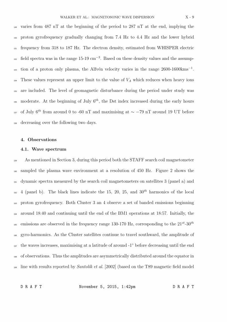
As mentioned in Section 3, during this period both the STAFF search coil magnetometer159

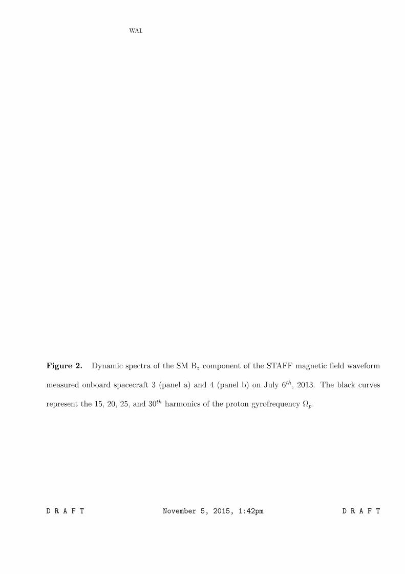
sampled the plasma wave environment at a resolution of 450 Hz. Figure 2 shows the160

dynamic spectra measured by the search coil magnetometers on satellites 3 (panel a) and161

4 (panel b). The black lines indicate the 15, 20, 25, and 30th harmonics of the local162

proton gyrofrequency. Both Cluster 3 an 4 observe a set of banded emissions beginning163

around 18:40 and continuing until the end of the BM1 operations at 18:57. Initially, the164

emissions are observed in the frequency range 130-170 Hz, corresponding to the 21st-30th165

gyro-harmonics. As the Cluster satellites continue to travel southward, the amplitude of166

the waves increases, maximising at a latitude of around -1 before decreasing until the end167

of observations. Thus the amplitudes are asymmetrically distributed around the equator in168

line with results reported by Santolık et al. [2002] (based on the T89 magnetic field model169



[Tsyganenko, 1989]).During this period, the external magnetic field weakens as evidenced170

by the decrease in the gyrofrequency harmonics. At the same time, the emission frequency171

of the waves drops, mirroring the change observed on the gyrofrequency harmonics. This172

frequency change is evidence that the waves are observed in their source region.173

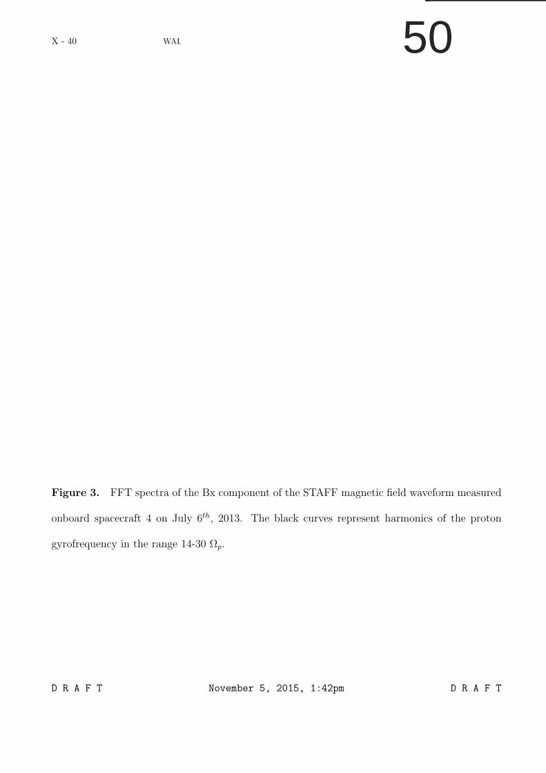
Figure 3 shows averaged spectra of the Cluster 4 STAFF search coil Bx (GSE) mea-174

surements centred at (top to bottom)18:43, 18:46, 18:51, and 18:56. Each spectrum is175

the average of 9 1024 point Fourier spectra. The vertical dotted black lines mark the176

14th − 30th harmonics of the local proton gryofrequency. It is noticeable that two types177

of emission can be seen in Figures 2 and 3. The first corresponds to the higher frequency178

emissions seen in the top three plots of Figure 3. These high frequency emissions occur179

close to harmonics of the local proton gyrofrequency in the range 20Ωp < ω < 30Ωp180

and as the magnetic field decreases so does the frequency of emission. The position of181

the peaks relative to the gyrofrequency harmonics changes with time. In panel (a) the182

majority of the spectral peaks are observed just below the gyroharmonics whilst in panel183

(b), corresponding to the time around the magnetic field line minimum, the peaks are184

at the gyro frequencies. As the spacecraft moves away from the field line minimum the185

frequency relative to the gyroharmonic falls.186

Figure 4 shows the FFT spectrum of emissions between 18:48:40 and 18:49:20 UT187

calculated by averaging nine 2048 point FFTs. The external magnetic field in this period188

varied from 339-335 nT (Ωp changes from 5.2-5.14 Hz). The format is the same as that in189

Figure 3. During this period, emission lines are observed in the frequency range from 14Ωp190

to 29Ωp. The position of the emission with respect to the harmonic frequency varies with191

harmonic number. At the low frequency end of the spectrum e.g. harmonics 14-18, the192



emissions occur at the exact frequency of the gyroharmonic whereas at higher frequencies193

the emissions lie slightly below the harmonic. In the case of the 23 and 24 harmonics194

the frequency difference is around 1.1 Hz. The other noticeable feature in this Figure is195

that most harmonics (except those mentioned above) exhibit multiple peaks. This could196

indicate the existence of further interactions with heavier ions such as He+, He2+, or O+197

ions. This harmonic structure implies that resonant interactions have a dominant role in198

the generation of these waves. This topic will be investigated further in a later paper.199

The second type of emissions is seen in Figures 2 and 3 (panel d), measured around200

18:56 UT. These emissions are observed in the frequency range 10-16Ωp. and occur be-201

tween the local gyroharmonics. Their frequency spacing is of the order of 4.3 Hz and202

analysis of spectra recorded after 18:56 UT (not shown). These emissions are monotonic,203

their frequency does not depend upon the local gyrofrequency. Emissions such as these204

are more typical of those discussed by other authors when they refer to magnetosonic205

waves or equatorial noise [e.g. Santolık et al., 2002]. The reason for their constant fre-206

quency is that these waves were generated at some other location and have propagated to207

the location in which they are observed. Since the frequency spacing of these emissions208

is lower than the local proton gyrofrequency these emissions are generated in a region of209

lower magnetic field strength (∼282 nT) most probably at a greater radial distance, and210

have propagated to the point at which they were observed. Unfortunately, these emissions211

were not observed on C3 due to a mode change a few seconds before.212

4.2. Ion distributions

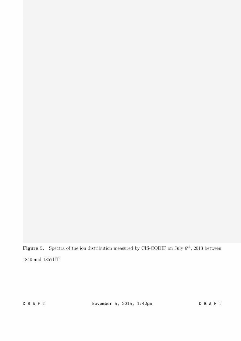
As noted in Section 1, the occurrence of magnetosonic waves are associated with ring-213

like ion distributions [Perraut et al., 1982; Chen et al., 2011]. Figure 5 shows the 1D214



ion distributions measured by CIS-CODIF instrument onboard Cluster 4. It should be215

noted that these observations are heavily contaminated due to the passage of the satellite216

through the radiation belts. In spite of this, evidence for the existence of a ring-like217

distribution is still very strong. The top panel shows the pitch-angle distribution of protons218

in the energy range 7-38.5 keV. These distributions are strongly peaked at pitch angles219

around 90, indicative of a ring-like distribution. During the period in which the waves220

are observed the particle flux observed increased, with the highest fluxes observed after221

1850UT corresponding to the period when emissions at high harmonics vanish whilst those222

at lower frequencies become less intense. This change in the distribution is also evident223

in the bottom panel which shows the particle count rate as a function of energy and time.224

The highest count rates are observed at energies above 10 keV, maximising in the region225

of 20-30 keV. This is the energy of the proton ring and corresponds to a velocity of the226

order Vr= 2000-2400 kms−1. This velocity is greater than the Alfven velocity (calculated227

in Section 3). Thus, the ring distribution could provide the free energy to enable the228

growth of the MSW since the energy of the ring distribution exceeds the Alfven energy229

[Korth et al., 1984]. Moving towards lower energies there is a distinct minimum in the230

energy just below the ring particles that occurs at an energy of around 7 keV. This energy,231

referred to as the dip energy/dip velocity (Vdip) [e.g. Chen et al., 2011], corresponds to232

a velocity of around 1100 kms−1. Thus, for velocities in the range Vdip < v⊥ < Vr the233

proton distribution has a positive gradient (∂f/∂v⊥ > 0).234

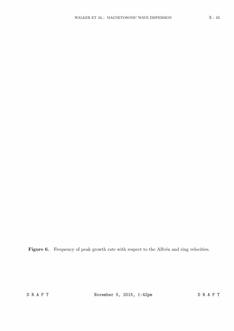
Using the results of the theoretical analysis performed by Chen et al. [2010], it is possible235

to estimate the frequencies at which the instability occurs and wave growth is observed.236

The blue curve in Figure 6 shows the approximate perpendicular velocity in terms of237



the Alfven velocity that corresponds to peak wave growth as a function of the harmonic238

resonance. Also plotted (black lines) are VA (dotted), Vdip (dashed), and Vr (dash-dotted).239

Thus it would be expected that there should be emission bands in the range 8-29Ωp since240

Vdip < v⊥ < Vr . The wave spectra, measured in the period 1844:45 to 1845:15 is shown241

in red. It is clear from this Figure that all harmonics at which waves were observed242

correspond to perpendicular velocities in the range Vdip < v⊥ < Vr, inline with results243

reported by Chen et al. [2010]. These results are consistent with the general trend reported244

by Ma et al. [2014]. From Figure 6 , the value of Vr/VA ∼ 1.02 which would imply that245

the unstable wave frequencies would be expected at frequencies around the mid-range of246

possible harmonics, exactly as was observed and shown in this figure.247

4.3. Wave Properties

In order to establish the propagation mode of the waves that were observed during this248

period the basic properties of these emissions were investigated based on the measurements249

from Cluster 4. In the previous Section it was shown that the bands of emission at higher250

frequencies typically occurred at or just below harmonics of the proton gyrofrequency. In251

this section, the wave polarisation and propagation characteristics are investigated.252

The wave properties for the period 18:47:00-18:47:20 UT, based on the STAFF search253

coil measurements, are shown in Figure 7. During this period, the proton gyrofrequency254

was 5.32 Hz. These results are based on the use of a Morlet wavelet transform to extract255

the frequency information from the waveform and Singular Valued Decomposition [San-256

tolik et al., 2003] to compute the eigenvectors and eigenvalues of the complex spectral257

matrix. It should be noted that the signal after 18:47:19 UT is superposed with a broad258



band signal arising from some local interference whose effects can be seen most clearly on259

the three lower panels.260

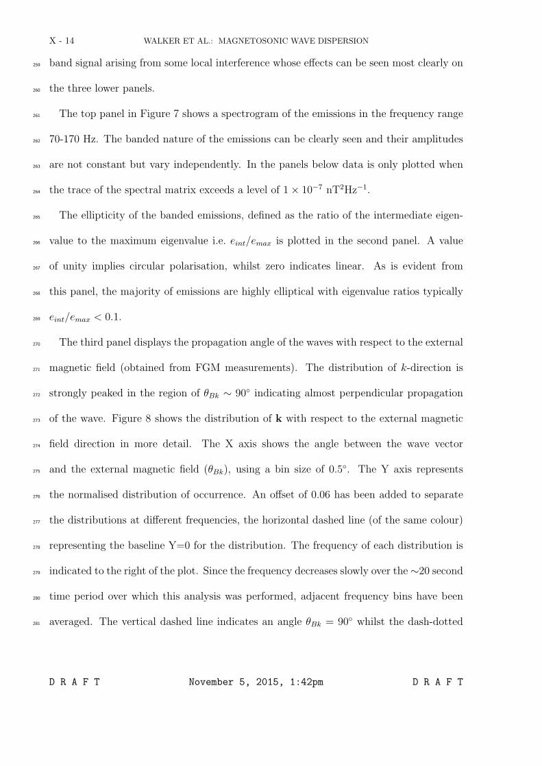
The top panel in Figure 7 shows a spectrogram of the emissions in the frequency range261

70-170 Hz. The banded nature of the emissions can be clearly seen and their amplitudes262

are not constant but vary independently. In the panels below data is only plotted when263

the trace of the spectral matrix exceeds a level of 1× 10−7 nT2Hz−1.264

The ellipticity of the banded emissions, defined as the ratio of the intermediate eigen-265

value to the maximum eigenvalue i.e. eint/emax is plotted in the second panel. A value266

of unity implies circular polarisation, whilst zero indicates linear. As is evident from267

this panel, the majority of emissions are highly elliptical with eigenvalue ratios typically268

eint/emax < 0.1.269

The third panel displays the propagation angle of the waves with respect to the external270

magnetic field (obtained from FGM measurements). The distribution of k-direction is271

strongly peaked in the region of θBk ∼ 90 indicating almost perpendicular propagation272

of the wave. Figure 8 shows the distribution of k with respect to the external magnetic273

field direction in more detail. The X axis shows the angle between the wave vector274

and the external magnetic field (θBk), using a bin size of 0.5. The Y axis represents275

the normalised distribution of occurrence. An offset of 0.06 has been added to separate276

the distributions at different frequencies, the horizontal dashed line (of the same colour)277

representing the baseline Y=0 for the distribution. The frequency of each distribution is278

indicated to the right of the plot. Since the frequency decreases slowly over the ∼20 second279

time period over which this analysis was performed, adjacent frequency bins have been280

averaged. The vertical dashed line indicates an angle θBk = 90 whilst the dash-dotted281



lines mark angles of θBk = 88.5 and θBk = 91.5. These plots show that the majority of282

the propagation angles occur in the range 87-93. There appears to be two basic types283

of distribution. The first show a peak at θBk = 90, indicating that the waves propagate284

perpendicularly to the external magnetic field. Such distributions are observed for waves285

of frequency 160.5, 150.5, 109.5, 107.5, and 92.5Hz. The second type of distribution286

exhibits a number of peaks in the angular distribution, indicating a preference for almost287

perpendicular propagation e.g. the distributions for frequencies 155.5, 113.5, 97.5, and288

86.5Hz. Typically, the peaks occur within 2 of perpendicular, a value in line with that289

often quoted in discussions of the propagation of magnetosonic waves.290

Finally, the fourth panel of Figure 7 displays the angle between the eigenvector of the291

magnetic field oscillations that corresponds to the maximum eigenvalue i.e. the direction292

of the principle axis of the polarisation ellipsoid and the direction of the external magnetic293

field. The distribution is centred on the direction antiparallel to the external magnetic294

field implying that the oscillations of the wave magnetic field occur in the direction parallel295

to the external magnetic field.296

In summary, the banded emissions observed by the Cluster 4 STAFF search coil magne-297

tometer during the period 18:47:00-18:47:20 UT are consistent with whistler mode waves298

propagating almost perpendicular to the eternal magnetic field since they are highly ellip-299

tical in nature and the wave magnetic field oscillates parallel to the external field. Thus300

these emissions are examples of magnetosonic waves (equatorial noise). This conclusion is301

further strengthened in the next sections by the determination of the dispersion relation302

of the observed waves and its comparison to dispersion relations derived theoretically.303



5. Experimental Determination of the Dispersion Relation

The wave vector (k) of a wave is a vector quantity whose direction corresponds to the304

wave propagation direction and whose magnitude is related to the wavelength (λ) of the305

wave (|k| = 2π/λ). Determination of the wave vector is important when considering the306

propagation of waves within the plasma environment as well as their interaction with307

the local particle populations for which they provide a medium for the transfer of energy308

between the particle populations via either current or resonant instabilities.309

Experimental determination of the wave vector has only been possible since the advent310

of multispacecraft missions and the possibility of making simultaneous measurements at311

two or more closely spaced points in space. Depending upon the type of data sets available,312

there are a number of different methods such as k-filtering/wave telescope [Pincon and313

Lefeuvre, 1992], and phase differencing [Balikhin and Gedalin, 1993; Balikhin et al., 1997a;314

Chisham et al., 1999] that may be employed. These methods, which were compared315

in Walker et al. [2004], are based on the fact that a comparison of the simultaneous316

multipoint measurements will show differences in the phase of the wave at the different317

measurement locations. These differences may then be used to determine the k-vector of318

the wave. In the present paper, the phase differencing methodology is employed.319

Following Balikhin et al. [1997b] and Balikhin et al. [2001] the basic assumption behind320

the phase differencing method is that the measured wave field may be represented by the321

superposition of plane waves as shown by equation (1)322

B(r, t) = ΣωBω exp[i(k · r− ωt)] + cc (1)323

where Bω is the wave amplitude at frequency ω, k is the wave vector (k-vector), r is the324

separation vector between the location of the two (or more) simultaneous measurements,325



and cc represents the complex conjugate term. A comparison of observations from two326

closely spaced locations will display a difference in the phases of the measurements of327

the wave. This phase shift ∆ψ is proportional to the component of the wave vector k328

projected along the measurement separation direction r (assuming that there is only one329

wave vector k for any frequency ω) and is given by (2).330

∆ψ(ω) = k(ω) · r+ 2nπ331

= ∥k∥∥r∥ cos(θkr) + 2nπ (2)332

where θkr is the angle between the wave vector k and the satellite separation vector r333

and n is an integer value. Since the phase difference between the two signals can only be334

determined in the range −π < ∆ψ < π, a family of periodic solutions is possible, resulting335

in a phase ambiguity of 2nπ. Thus, in order to determine the correct value of kr it is336

necessary to determine the correct value of n.337

The phase differencing method may be applied to scalar measurements or single com-338

ponents of a vector quantity and results in a measurement of the component of the wave339

vector projected along the measurement separation vector. If measurements are available340

from four (or more) closely spaced, non-coplanar locations it is possible to determine the341

projection of the wave vector along three independent directions and hence determine the342

complete wave vector [Balikhin et al., 2003]. However, if measurements from only two343

locations are available the size of kr can be estimated but not it’s direction and so another344

method is required to determine the direction of k. One such method that may be used345

with magnetic field data is to calculate the eigenvalues and eigenvectors of the magnetic346

field covariance matrix. Provided that the ratio of the intermediate to minimum eigenval-347

ues is large (typically a factor 10, i.e. the wave is not linearly polarised) then the minimum348



variance direction is well defined and represents the direction of wave propagation. Thus,349

knowledge of the direction together with the magnitude of k-vector projected along the350

measurement separation vector enables the full wave k-vector to be determined.351

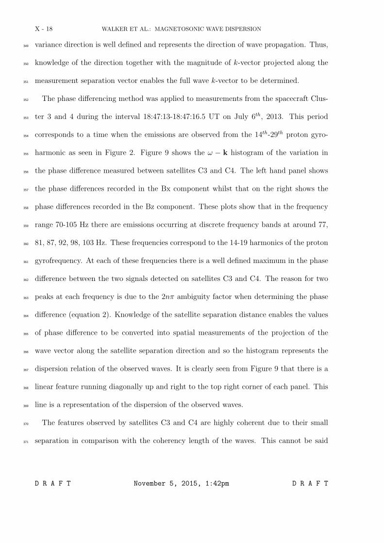
The phase differencing method was applied to measurements from the spacecraft Clus-352

ter 3 and 4 during the interval 18:47:13-18:47:16.5 UT on July 6th, 2013. This period353

corresponds to a time when the emissions are observed from the 14th-29th proton gyro-354

harmonic as seen in Figure 2. Figure 9 shows the ω − k histogram of the variation in355

the phase difference measured between satellites C3 and C4. The left hand panel shows356

the phase differences recorded in the Bx component whilst that on the right shows the357

phase differences recorded in the Bz component. These plots show that in the frequency358

range 70-105 Hz there are emissions occurring at discrete frequency bands at around 77,359

81, 87, 92, 98, 103 Hz. These frequencies correspond to the 14-19 harmonics of the proton360

gyrofrequency. At each of these frequencies there is a well defined maximum in the phase361

difference between the two signals detected on satellites C3 and C4. The reason for two362

peaks at each frequency is due to the 2nπ ambiguity factor when determining the phase363

difference (equation 2). Knowledge of the satellite separation distance enables the values364

of phase difference to be converted into spatial measurements of the projection of the365

wave vector along the satellite separation direction and so the histogram represents the366

dispersion relation of the observed waves. It is clearly seen from Figure 9 that there is a367

linear feature running diagonally up and right to the top right corner of each panel. This368

line is a representation of the dispersion of the observed waves.369

The features observed by satellites C3 and C4 are highly coherent due to their small370

separation in comparison with the coherency length of the waves. This cannot be said371



for the observations by Cluster 1, whilst Cluster 2 is in a completely different plasma372

location and does not see this banded structures at all. It is, therefore, not possible to373

use the phase differencing technique to determine the dispersion relations between other374

pairs of satellites in the Cluster quartet and hence compute the full k-vector. In order375

to find the direction of the wave k-vector another method is required. Since the above376

analysis is based on magnetic field measurements it is possible to obtain the direction of377

k by calculating the eigenvalues and corresponding eigenvectors of the magnetic field co-378

variance matrix. The analysis period (18:47:13-18:47:16.5 UT) was divided into a number379

of segments, each typically 0.25 seconds, and the eigenvalues and vectors were calculated.380

The direction of k was taken as the average of the minimum variance directions for which381

the corresponding ratio of the intermediate to minimum eigenvalues λint/λmin > 50. This382

criteria ensures that the minimum variance direction is well defined. This direction, to-383

gether with the projections of k along the satellite separation vector were used to compute384

the k-vector of the wave.385

However, this still leaves the problem of resolving the ambiguity factor 2nπ in the386

determination of the phase difference between the two signals. There are two scenarios387

for which the determination of n is reasonably straight forward. The first is for low388

frequency signals, i.e. those whose wavelength is much greater than the separation of the389

two measurement points in which case n would probably be zero and the phase difference390

could actually be computed directly from the waveforms [e.g. Balikhin et al., 1997c]. The391

second scenario involves the comparison of isolated wave packets whose waveforms are392

virtually identical in both signals [e.g. Balikhin et al., 2005]. Neither of these methods393

could be applied to the current case in question since the observed waves consist of a394



superposition of waves with a number of discrete frequencies and variable amplitudes.395

This fact also rules out the possibility of determining n from the shape of sequences of wave396

packets since they are just too irregular [Walker and Moiseenko, 2013]. Therefore, the397

only way to determine n is to compare the experimental dispersion with one determined398

from theory and match the two by changing the value of n.399

6. Theoretical insight into the propagation of MSW

To get some insight into the properties of MSW it is instructive to consider the theoret-400

ical derivation of their dispersion relation, growth rate and propagation direction based401

on the local ion distribution. The contribution of the ions to the growth rate of MSW402

is investigated based on an approach first proposed about fifty years ago [Dawson, 1961;403

O’Neil , 1965] and has since been used for many studies of wave-particle interactions in404

the magnetosphere. This approach assumes the magnetospheric plasma is composed of405

two parts: a “cold” bulk population of electrons and ions that determines the plasma406

dispersion relation, and low-density suprathermal populations of electrons and ions which407

participate in resonant interactions with the waves and are responsible for wave growth408

or damping. If the wave growth (or damping) rate is less than the inverse nonlinear time409

of resonant interaction, the resonant particle distribution function can be found using the410

adiabatic approximation with respect to the wave amplitude, i.e. neglecting the amplitude411

variation during the time of resonant interaction.412

6.1. Dispersion relation and polarization of magnetosonic waves below ωLH

The electric field of a plane wave can be written as413

E = ReaEei(kr−ωt) (3)414



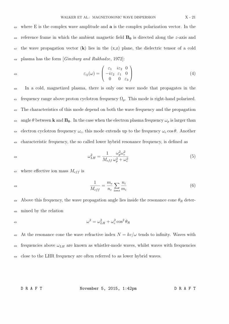
where E is the complex wave amplitude and a is the complex polarization vector. In the415

reference frame in which the ambient magnetic field B0 is directed along the z-axis and416

the wave propagation vector (k) lies in the (x,z) plane, the dielectric tensor of a cold417

plasma has the form [Ginzburg and Rukhadze, 1972]:418

εij(ω) =

ε1 iε2 0−iε2 ε1 00 0 ε3

(4)419

In a cold, magnetized plasma, there is only one wave mode that propagates in the420

frequency range above proton cyclotron frequency Ωp. This mode is right-hand polarized.421

The characteristics of this mode depend on both the wave frequency and the propagation422

angle θ between k andB0. In the case when the electron plasma frequency ωp is larger than423

electron cyclotron frequency ωc, this mode extends up to the frequency ωc cos θ. Another424

characteristic frequency, the so called lower hybrid resonance frequency, is defined as425

ω2LH =

1

Meff

ω2pω

2c

ω2p + ω2

c

(5)426

where effective ion mass Meff is427

1

Meff

=me

ne

∑ions

ni

mi

(6)428

Above this frequency, the wave propagation angle lies inside the resonance cone θR deter-429

mined by the relation430

ω2 = ω2LH + ω2

c cos2 θR431

At the resonance cone the wave refractive index N = kc/ω tends to infinity. Waves with432

frequencies above ωLH are known as whistler-mode waves, whilst waves with frequencies433

close to the LHR frequency are often referred to as lower hybrid waves.434



Below the LHR frequency, the propagation angle is arbitrary, including θ = π/2. In435

this frequency range the propagating right-hand polarized waves are often termed mag-436

netosonic waves.437

For waves in the frequency range438

Ωp ≪ ω ∼< ωLH ≪ ωc439

and assuming ωp ≫ ωc the real part of the quantities ε1, ε2, and ε3 can be approximated440

by441

ε1 ≃ω2p + ω2

c

ω2c

(1− ω2

LH

ω2

); ε2 ≃ −

ω2p

ωωc

; ε3 ≃ −ω2p

ω2.442

Note that in this frequency range, the ions only contribute to the quantity ε1, through the443

term ω2LH , while the quantities ε2 and ε3 are determined solely by the electrons. Using444

general dispersion relation for electromagnetic waves in a cold magnetized plasma [see445

e.g. Ginzburg and Rukhadze, 1972], together with the expressions for the components of446

the dielectric tensor given above, one can derive the following dispersion relation in the447

frequency range of interest [Shklyar and Jirıcek , 2000]448

ω2 =ω2LH

1 + q2/k2+

ω2c cos

2 θ

(1 + q2/k2)2≡ ω2

LH

k2

k2 + q2+ ω2

c

k2∥k2

(k2 + q2)2, (7)449

where450

q2 =ω2p

c2, (8)451

and k∥ = k cos θ and k⊥ = k sin θ. Figure 10 shows the so-called surface of the refractive452

index, i.e. the isolines of constant frequencies on the (k⊥, k∥)-plane, resulting from the453

dispersion relation (7). The contours shown correspond (from blue (inner) to brown454

(outer)) to the 14th, 17th, 20th, 23rd, 26th, and 29th harmonics of the proton cyclotron455

frequency. One can see that for any frequency, the largest possible value of k∥ corresponds456



to parallel propagation, i.e., k = k∥ , k⊥ = 0 ; and since for ω ∼< ωLH , each term on the457

right hand side of (7) is smaller than ω2LH , so that the following inequalities should be458

fulfilled:459

k2∥q2

<ω

ωc∼<ωLH

ωc

≪ 1 ;k2

q2<

ω2

ω2LH − ω2

. (9)460

Due to reasons clarified below, only waves propagating at a large angle θ to the ambient461

magnetic field will be considered.462

In order to estimate typical values for the refractive index, the maximum parallel com-463

ponent of the wave vector, and the resonant velocity the following further assumptions464

are made. As can be seen from Figure 10, for ω ∼< ωLH , the wave refractive index N at465

large θ is of the same order as its value at θ = π/2 (which is not true for ω = ωLH). From466

(7) it then follows that in the case under discussion k2 ∼ ω2p/c

2, or alternatively467

N2 ∼ω2p

ω2. (10)468

Using the standard relations between the components of the polarization vector a [see e.g.469

Shklyar and Matsumoto, 2009]470

ay = −i ε2N2 − ε1

ax ; az =N2 sin θ cos θ

N2 sin2 θ − ε3ax , (11)471

and the expressions for ε1 , ε2 , ε3 given previously the polarisation vector can be rewritten472

as473

ay ∼ iω

ωc

ax ≪ ax ; az ∼ cos θ ax ≪ ax ,474

so that the wave electric field is right-hand and almost linearly polarized along the x-axis.475

As for the wave magnetic field, combining Faraday’s law [k × E] = (ω/c)B and the476

relations given above it follows that477

|Bx| ∼ωp

ωc

cos θ ax|E| ; |By| ∼ωp

ωcos θ ax|E| ; |Bz| ∼

ωp

ωc

sin θ ax|E| ,478



thus, |Bx| ≪ |By| , |Bz|. It is worth mentioning that |B| ≫ |E| (in CGS units), but479

|B| ≪ N |E|.480

6.2. Propagation of magnetosonic waves in the magnetosphere

The surface of the refractive index, shown in Figure 10, provides information regarding481

the propagation on MSW. Since the wave group velocity is directed normal to the refractive482

index surface, for large θ except when considering propagation directions close to θ = π/2,483

the wave group velocity is directed almost along the ambient magnetic field. In the vicinity484

of θ = π/2, the direction of wave group velocity with respect to the ambient magnetic field485

changes sign very fast, so that the point where θ = π/2 may be considered as a reflection486

point. Figure 11 shows an example of the ray trajectory of a 150 Hz magnetosonic wave487

propagating in meridian plane which starts at L = 4.15 on the equator and has a wave488

normal angle θ0 = 89. We see that the latitude of the ray trajectory oscillates around489

zero, so that the trajectory as the whole is confined to the equatorial region. If the initial490

wave normal angle has an azimuthal component, the ray no longer lies in the meridian491

plane, but its confinement to the equatorial region remains in effect.492

6.3. Magnetosonic wave excitation

Considering MSW excitation as the result of resonant interaction with energetic plasma493

particles, assuming cyclotron instability to be in effect the resonant velocity related to the494

nth cyclotron resonance is given by495

VRnα =ω − nωHα

k∥, α = e, i (12)496

where index α refers to quantities related to electrons (e) and protons (i), so that ωHe = ωc497

and ωHi = Ωp. Equation (12) defines the particle parallel velocity at which it interacts498



resonantly with the wave. Since the waves are excited due to their interaction with499

resonant particles, and because the number of these particles depends on their energy500

and in particular their parallel velocity, the value of VRnα is essential for estimating the501

efficiency of their interaction. The value of VRnα may be estimated using the following502

parameters, which are typical of the equatorial region at L = 4.15, namely:503

ω ∼ 900 rad/s ; ωp ∼ 6.4·105 rad/s ; ωc ∼ 7.6·104 rad/s ; Ωc ∼ 41.6 rad/s ; ωLH ∼ 1.8·103 rad/s504

together with (see (10))505

N ∼ 677 ; k ∼ 2.1 · 10−5cm−1 . (13)506

The first inequality in (9) gives the maximum value of k∥507

(k∥)max ∼ 2.4 · 10−6cm−1 .508

Obviously, this value corresponds to the parallel propagation of MSW. Using this value509

we find that, in general510

|VR1e| > 3.2 · 1010cm/s ; VR1i > 3.8 · 108cm/s ; VR0 > 4 · 108cm/s .511

Note that the Cerenkov resonance velocity (VR0) does not depend on the type of particle,512

in contrast to cyclotron resonance velocities.513

Relation (12) is written using the non-relativistic approximation. In this approximation,514

it may be seen that the interaction of MSW with electrons at the first cyclotron resonance515

- the only one that exists for parallel propagation - is impossible. As for the protons,516

the value of V∥ = VR1i corresponds to proton energies exceeding 100 keV, and so only a517

small number of resonant particles may be expected in this case. Thus, it is necessary518

to consider oblique MSW propagation. In this case the Cerenkov resonance comes into519



effect, playing the main role together with the first cyclotron resonance, for small and520

medium wave normal angles. For oblique propagation, the value of VR0 given above521

represents the minimum value of parallel velocity, corresponding to E > 65 eV electrons522

and E > 118 keV ions. In the absence of parallel beams, the Cerenkov resonance leads to523

wave damping and, given the relation between resonance energies, drives out a possible524

wave excitation at the first cyclotron resonance due to cyclotron instability. Thus, the525

only possible case for MSW excitation is when k∥ ≪ (k∥)max, i.e., when the wave normal526

angle is close to π/2 and ω ≃ nΩc. In this case, the Cerenkov resonance for electrons does527

not drive out the instability, since it corresponds to an overly high electron velocity, while528

VRni for protons can be sufficiently small for an appropriate number of particles to be in529

cyclotron resonance. As was shown by Shklyar [1986], higher order cyclotron resonances530

for protons are efficient only when531

k∥V∥ + k⊥V⊥ > ω ,532

which requires V⊥ > ω/k. Using (13) it is found that V⊥ > 4.5 · 107cm/s, or E > 1 keV,533

which is quite realistic for protons.534

A general expression for the growth rate of the cyclotron instability for oblique elec-535

tromagnetic wave, which is valid for MSW under consideration, can be found in Shklyar536

and Matsumoto [2009, expression (4.13)]. As has been argued above, the growth rate is537

significant only for ω ≃ nΩc, with the main contribution to the growth rate from protons538

interacting with the wave at the nth cyclotron resonance. Retaining the corresponding539

term for the growth rate from Shklyar and Matsumoto [2009] it is found that540

γ =Ωc(πe|E|c)2

2mik∥U

∫ ∞

0dµf ′

0n(µ)V2n (µ) , (14)541



where f0 is the unperturbed proton distribution function, which depends on particle energy542

W and magnetic momentum µ,543

f ′0n =

(∂f0∂W

+n

ω

∂f0∂µ

)W=miV 2

Rni/2+µΩc

, (15)544

545

Vn =

(n|Ωc|k⊥c

ax +VRni

caz

)Jn(ρ) +

iρΩc

k⊥cayJ

′n(ρ) ; ρ = k⊥

(2µ

mi|Ωc|

)1/2

, (16)546

and Jn(ρ) and J′n(ρ) are, respectively, the Bessel function and its derivative with respect547

to the argument ρ. The quantity ρ defined above is the dimensionless Larmor radius, i.e.,548

ρ = k⊥V⊥/Ωc. The quantity U that enters the expression for γ is the wave energy density549

and is proportional to |E|2 and expressed through the polarization coefficients and the550

dielectric tensor in a usual way [e.g. Shafranov , 1967]. The value of Vn, which plays the551

role of an effective amplitude of interaction at the nth cyclotron resonance is proportional552

to Jn(ρ). It is well known that for large n this function is exponentially small unless553

ρ ≡ k⊥V⊥/Ωc > n, or, with the account of n ≃ ω/Ωc, k⊥V⊥ > ω . This explains the above554

mentioned requirement of the efficiency of wave excitation by ions.555

From (14)-(16) it follows that for wave excitation the derivative (15) should, on average,556

be positive, which is typically observed for distributions with a loss-cone or temperature557

anisotropy. In general, the growth rate strongly depends on the energetic proton distribu-558

tion function, as well as on the wave characteristics (frequency and wave vector). However,559

in many cases the distribution function is proportional to exp(−W/WT ), where WT is a560

characteristic energy scale of the distribution. (For a quasi-Maxwellian distribution, WT561

characterizes the particle thermal energy). In this case, the growth rate γ defined by (14)562

appears to be proportional to563

exp

−mi(ω − nΩc)2

2k2∥WT

564



As mentioned above, k∥ is a small quantity, which clearly shows that the growth rate is565

significant only for ω ≃ nΩc, i.e., for frequencies close to ion cyclotron harmonics.566

6.4. Comparison of Experimental and Theoretical Dispersion

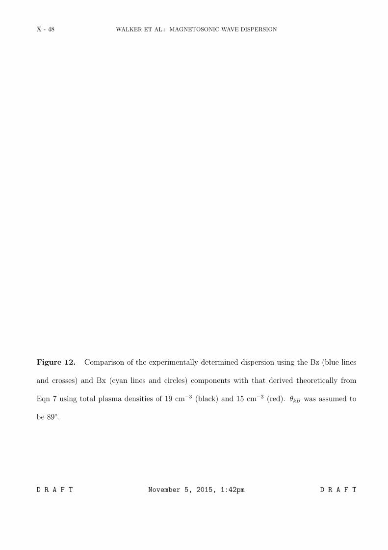
The dispersion relation (7) is plotted as the solid line in Figure 12 using plasma densities567

of 19 cm−3 (black) and 15 cm−3 estimated using data from WHISPER. The angle between568

the wave propagation vector and the eternal magnetic field was assumed to be 89. In569

order to fit the experimentally derived dispersion to the theoretical ones n, the ambiguity570

factor in equation (2) was varied in the range −5 < n < 5 and the results compared to571

the theoretical curves. It was found that the best fit was obtained using n = 1 and the572

dispersions of the Bx (blue crosses) and Bz (cyan circles) components using this factor573

are shown in the Figure. This value is in agreement with the fact that the wavelength of574

the magnetosonic waves is ∼18 km (from the dispersion shown in Figure 12) compared575

with an intersatellite separation of 60 km. As can be seen from this Figure there is good576

agreement between the experimental and theoretical results.577

7. Conclusions

Using data collected as part of the Cluster Inner Magnetosphere campaign this paper has578

presented observations of a set of narrow banded emissions that occurred in the vicinity of579

harmonics of the proton gyrofrequency. It was demonstrated that these waves propagated580

in the magnetosonic mode as characterised by their spectral properties.581

Using the phase differencing method, it was possible to combine observations from the582

satellites Cluster 3 and Cluster 4 in order to determine the dispersion relation. The exper-583



imentally determined dispersion was shown to be consistent with theoretical dispersion584

curves.585

Acknowledgments. SNW and MAB wish to acknowledge financial support from In-586

ternational Space Science Institute, Bern, Royal Society Collaboration grant, UK EPSRC587

grant EP/H00453X/1, and the European Union’s Horizon 2020 research and innovation588

programme under grant agreement No 637302. The authors would like to thank the Clus-589

ter instrument teams for provision of the data used in this paper. These data are available590

from the Cluster Science Archive (http://www.cosmos.esa.int/web/csa).591

References

Albert, J. M. (2008), Efficient approximations of quasi-linear diffusion coefficients592

in the radiation belts, J. Geophys. Res. (Space Physics), 113, A06208, doi:593

10.1029/2007JA012936.594

Andre, R., F. Lefeuvre, F. Simonet, and U. S. Inan (2002), A first approach to model the595

low-frequency wave activity in the plasmasphere, Annales Geophysicae, 20, 981–996,596

doi:10.5194/angeo-20-981-2002.597

Balikhin, M., S. Walker, R. Treumann, H. Alleyne, V. Krasnoselskikh, M. Gedalin, M. An-598

dre, M. Dunlop, and A. Fazakerley (2005), Ion sound wave packets at the quasiperpen-599

dicular shock front, Geophys. Res. Lett., 32 (24), L24,106, doi:10.1029/2005GL024660.600

Balikhin, M. A., and M. E. Gedalin (1993), Comparative analysis of different methods601

for distinguishing temporal and spatial variations, in Proc. of START Conf., Aussois,602

France, vol. ESA WPP 047, pp. 183–187.603

Balikhin, M. A., L. J. C. Woolliscroft, H. S. Alleyne, M. Dunlop, and M. A. Gedalin604



(1997a), Determination of the dispersion of low frequency waves downstream of a quasi-605

perpendicular collisionless shock, Annales Geophysicae, 15 (2), 143–151.606

Balikhin, M. A., T. Dudok de Witt, L. J. C. Woolliscroft, S. N. Walker, H. Alleyne,607

V. Krasnoselskikh, W. A. C. Mier–Jedrzejowicz, and W. Baumjohann (1997b), Ex-608

perimental determination of the dispersion of waves observed upstream of a quasi–609

perpendicular shock, Geophys. Res. Lett., 24, 787–790, doi:10.1029/97GL00671.610

Balikhin, M. A., S. N. Walker, T. Dudok de Witt, H. S. Alleyne, L. J. C. Woolliscroft,611

W. A. C. Mier-Jedrzejowicz, and W. Baumjohann (1997c), Nonstationarity and low612

frequency turbulence at a quasi-perpendicular shock front, Adv. Sp. Res., 20 (4-5), 729–613

734, doi:10.1016/S0273-1177(97)00463-8.614

Balikhin, M. A., S. Schwartz, S. N. Walker, H. S. C. K. Alleyne, M. Dunlop, and H. Luhr615

(2001), Dual-spacecraft observations of standing waves in the magnetosheath, J. Geo-616

phys. Res., 106 (A11), 25,395–25,408, doi:10.1029/2000JA900096.617

Balikhin, M. A., O. A. Pokhotelov, S. N. Walker, E. Amata, M. Andre, M. Dunlop,618

and H. S. K. Alleyne (2003), Minimum variance free wave identification: Application619

to Cluster electric field data in the magnetosheath, Geophys. Res. Lett., 30 (10), 15-1,620

doi:10.1029/2003GL016918.621

Balikhin, M. A., Y. Y. Shprits, S. N. Walker, L. Chen, N. Cornilleau-Wehrlin,622

I. Dandouras, O. Santolik, C. Carr, K. H. Yearby, and B. Weiss (2015), Observa-623

tions of discrete harmonics emerging from equatorial noise, Nat Commun, 6, doi:624

10.1038/ncomms8703.625

Balogh, A., M. W. Dunlop, S. W. H. Cowley, D. J. Southwood, J. G. Thomlinson, K. H.626

Glassmeier, G. Musmann, H. Luhr, S. Buchert, M. H. Acuna, D. H. Fairfield, J. A.627



Slavin, W. Riedler, K. Schwingenschuh, and M. G. Kivelson (1997), The Cluster mag-628

netic field investigation, Sp. Sci. Rev., 79, 65–91, doi:10.1023/A:1004970907748.629

Boardsen, S. A., D. L. Gallagher, D. A. Gurnett, W. K. Peterson, and J. L. Green630

(1992), Funnel-shaped, low-frequency equatorial waves, J. Geophys. Res., 97, 14,967,631

doi:10.1029/92JA00827.632

Boardsen, S. A., G. B. Hospodarsky, C. A. Kletzing, R. F. Pfaff, W. S. Kurth, J. R.633

Wygant, and E. A. MacDonald (2014), Van Allen Probe observations of periodic rising634

frequencies of the fast magnetosonic mode, Geophys. Res. Lett., 41, 8161–8168, doi:635

10.1002/2014GL062020.636

Bortnik, J., and R. M. Thorne (2010), Transit time scattering of energetic electrons due637

to equatorially confined magnetosonic waves, J. Geophys. Res. (Space Physics), 115,638

A07213, doi:10.1029/2010JA015283.639

Chen, L., and R. M. Thorne (2012), Perpendicular propagation of magnetosonic waves,640

Geophys. Res. Lett., 39, L14102, doi:10.1029/2012GL052485.641

Chen, L., R. M. Thorne, V. K. Jordanova, and R. B. Horne (2010), Global simulation642

of magnetosonic wave instability in the storm time magnetosphere, J. Geophys. Res.643

(Space Physics), 115 (A11), A11222, doi:10.1029/2010JA015707.644

Chen, L., R. M. Thorne, V. K. Jordanova, M. F. Thomsen, and R. B. Horne (2011),645

Magnetosonic wave instability analysis for proton ring distributions observed by the646

lanl magnetospheric plasma analyzer, J. Geophys. Res. (Space Physics), 116, A03223,647

doi:10.1029/2010JA016068.648

Chisham, G., S. J. Schwartz, M. Balikhin, and M. W. Dunlop (1999), AMPTE obser-649

vations of mirror mode waves in the magnetosheath: Wavevector determination, J.650



Geophys. Res. A, 104 (A1), 437–447, doi:10.1029/1998JA900044.651

Cornilleau-Wehrlin, N., P. Chauveau, S. Louis, A. Meyer, J. M. Nappa, S. Perraut,652

L. Rezeau, P. Robert, A. Roux, C. De Villedary, Y. de Conchy, L. Friel, C. C. Har-653

vey, D. Hubert, C. Lacombe, R. Manning, F. Wouters, F. Lefeuvre, M. Parrot, J. L.654

Pincon, B. Poirier, W. Kofman, P. Louarn, and the STAFF Investigator Team (1997),655

The Cluster Spatio-Temporal Analysis of Field Fluctuations (STAFF) experiment, Sp.656

Sci. Rev., 79, 107–136.657

Dawson, J. (1961), On landau damping, Phys. Fluids, 4, 869–874, doi:10.1063/1.1706419.658

Decreau, P. M. E., P. Fergeau, V. Krannosels’kikh, M. Leveque, P. Martin, O. Ran-659

driamboarison, F. X. Sene, J. G. Trotignon, P. Canu, and P. B. Mogensen (1997),660

WHISPER, a resonance sounder and wave analyser: Performances and perspectives for661

the Cluster mission, Sp. Sci. Rev., 79, 157–193, doi:10.1023/A:1004931326404.662

Fu, H. S., J. B. Cao, Z. Zhima, Y. V. Khotyaintsev, V. Angelopoulos, O. Santo-663

lik, Y. Omura, U. Taubenschuss, L. Chen, and S. Y. Huang (2014), First observa-664

tion of rising-tone magnetosonic waves, Geophys. Res. Lett., 41 (21), 7419–7426, doi:665

10.1002/2014GL061687.666

Ginzburg, V. L., and A. A. Rukhadze (1972), Waves in magnetoactive plasma, in Handbook667

of Physics, vol. 49, edited by S. Flugge, p. 395, Springer, Berlin.668

Gurnett, D. A. (1976), Plasma wave interactions with energetic ions near the magnetic669

equator, J. Geophys. Res., 81, 2765–2770, doi:10.1029/JA081i016p02765.670

Gurnett, D. A., R. L. Huff, and D. L. Kirchner (1997), The wide-band plasma wave671

investigation, Sp. Sci. Rev., 79, 195–208.672



Gustafsson, G., R. Bostrom, B. Holback, G. Holmgren, A. Lundgren, K. Stasiewicz,673

L. Aehlen, F. S. Mozer, D. Pankow, P. Harvey, P. Berg, R. Ulrich, A. Pedersen,674

R. Schmidt, A. Butler, A. W. C. Fransen, D. Klinge, M. Thomsen, C.-G. Faltham-675

mar, P.-A. Lindqvist, S. Christenson, J. Holtet, B. Lybekk, T. A. Sten, P. Tanskanen,676

K. Lappalainen, and J. Wygant (1997), The Electric Field and Wave experiment for677

the Cluster mission, Sp. Sci. Rev., 79, 137–156.678

Horne, R. B., G. V. Wheeler, and H. S. C. K. Alleyne (2000), Proton and electron heating679

by radially propagating fast magnetosonic waves, J. Geophys. Res., 105, 27,597–27,610,680

doi:10.1029/2000JA000018.681

Horne, R. B., R. M. Thorne, S. A. Glauert, N. P. Meredith, D. Pokhotelov, and O. Santolık682

(2007), Electron acceleration in the Van Allen radiation belts by fast magnetosonic683

waves, Geophys. Res. Lett., 34, L17,107, doi:10.1029/2007GL030267.684

Kasahara, Y., H. Kenmochi, and I. Kimura (1994), Propagation characteristics of the elf685

emissions observed by the satellite akebono in the magnetic equatorial region, Radio686

Sci., 29, 751–767, doi:10.1029/94RS00445.687

Korth, A., G. Kremser, A. Roux, S. Perraut, J.-A. Sauvaud, J.-M. Bosqued, A. Peder-688

sen, and B. Aparicio (1983), Drift boundaries and ulf wave generation near noon at689

geostationary orbit, Geophys. Res. Lett., 10, 639–642, doi:10.1029/GL010i008p00639.690

Korth, A., G. Kremser, S. Perraut, and A. Roux (1984), Interaction of particles with ion691

cyclotron waves and magnetosonic waves. observations from GEOS 1 and GEOS 2.,692

Planet. Sp. Sci., 32 (11), 1393–1406.693

Laakso, H., H. Junginger, R. Schmidt, A. Roux, and C. de Villedary (1990), Magnetosonic694

waves above fc(H+) at geostationary orbit - GOES 2 results, J. Geophys. Res., 95,695



10,609–10,621, doi:10.1029/JA095iA07p10609.696

Ma, Q., W. Li, L. Chen, R. M. Thorne, and V. Angelopoulos (2014), Magnetosonic wave697

excitation by ion ring distributions in the earth’s inner magnetosphere, J. Geophys. Res.698

(Space Physics), 119, 844–852, doi:10.1002/2013JA019591.699

Meredith, N. P., R. B. Horne, and R. R. Anderson (2008), Survey of magnetosonic waves700

and proton ring distributions in the earth’s inner magnetosphere, J. Geophys. Res.701

(Space Physics), 113 (A6), A06213, doi:10.1029/2007JA012975.702

Mourenas, D., A. V. Artemyev, O. V. Agapitov, and V. Krasnoselskikh (2013), Analytical703

estimates of electron quasi-linear diffusion by fast magnetosonic waves, J. Geophys. Res.704

(Space Physics), 118, 3096–3112, doi:10.1002/jgra.50349.705

Nemec, F., O. Santolık, K. Gereova, E. Macusova, Y. de Conchy, and N. Cornilleau-706

Wehrlin (2005), Initial results of a survey of equatorial noise emissions observed by the707

Cluster spacecraft, Planet. Sp. Sci., 53, 291–298, doi:10.1016/j.pss.2004.09.055.708

Nemec, F., O. Santolık, Z. Hrbackova, J. S. Pickett, and N. Cornilleau-Wehrlin (2015),709

Equatorial noise emissions with quasiperiodic modulation of wave intensity, J. Geophys.710

Res. (Space Physics), 120, 2649–2661, doi:10.1002/2014JA020816.711

O’Neil, T. (1965), Collisionless damping of nonlinear plasma oscillations, Phys. Fluids, 8,712

2255–2262, doi:10.1063/1.1761193.713

Pedersen, A., N. Cornilleau-Wehrlin, B. De La Porte, A. Roux, A. Bouabdellah, P. M. E.714

Decreau, F. Lefeuvre, F. X. Sene, D. Gurnett, R. Huff, G. Gustafsson, G. Holmgren,715

L. Woolliscroft, H. S. Alleyne, J. A. Thompson, and P. H. N. Davies (1997), The Wave716

Experiment Consortium (WEC), Sp. Sci. Rev., 79, 93–106.717



Perraut, S., A. Roux, P. Robert, R. Gendrin, J. A. Sauvaud, J. M. Bosqued, G. Kremser,718

and A. Korth (1982), A systematic study of ulf waves above fH+ from geos 1 and 2719

measurements and their relationship with proton ring distributions, J. Geophys. Res.720

A, 87, 6219.721

Pincon, J.-L., and F. Lefeuvre (1992), The application of the generalized Capon method722

to the analysis of a turbulent field in space plasma: Experimental constraints, J. Atmos.723

Terr. Phys., 54, 1237–1247.724

Reme, H., J. M. Bosqued, J. A. Sauvaud, A. Cros, J. Dandouras, C. Aoustin, J. Bouys-725

sou, T. Camus, J. Cuvilo, C. Martz, J. L. Medale, H. Perrier, D. Romefort, J. Rouzaud,726

D. D’Uston, E. Mobius, K. Crocker, M. Granoff, L. M. Kistler, M. Popecki, D. Hov-727

estadt, B. Klecker, G. Paschmann, M. Scholer, C. W. Carlson, D. W. Curtis, R. P.728

Lin, J. P. McFadden, V. Formisano, E. Amata, M. B. Bavassano-Cattaneo, P. Baldetti,729

G. Belluci, R. Bruno, G. Chionchio, A. di Lellis, E. G. Shelley, A. G. Ghielmetti,730

W. Lennartsson, A. Korth, U. Rosenbauer, R. Lundin, S. Olsen, G. K. Parks, M. Mc-731

Carthy, and H. Balsiger (1997), The Cluster ion spectrometry (cis) experiment, Sp. Sci.732

Rev., 79, 303–350, doi:10.1023/A:1004929816409.733

Roberts, C. S., and M. Schulz (1968), Bounce resonant scattering of particles trapped in734

the Earth’s magnetic field, J. Geophys. Res., 73 (23), 7361–7376.735

Russell, C. T., R. E. Holzer, and E. J. Smith (1970), OGO 3 observations of ELF noise736

in the magnetosphere: 2. the nature of the equatorial noise, J. Geophys. Res., 75, 755,737

doi:10.1029/JA075i004p00755.738

Santolık, O., J. S. Pickett, D. A. Gurnett, M. Maksimovic, and N. Cornilleau-Wehrlin739

(2002), Spatiotemporal variability and propagation of equatorial noise observed by Clus-740



ter, J. Geophys. Res. A, 107 (A12), 43–1, doi:10.1029/2001JA009159.741

Santolik, O., M. Parrot, and F. Lefeuvre (2003), Singular value decomposition methods742

for wave propagation analysis, Radio Sci., 38 (1), 10–1, doi:10.1029/2000RS002523.743

Shafranov, V. D. (1967), Electromagnetic waves in a plasma, Reviews of Plasma Physics,744

3, 1.745

Shklyar, D., and H. Matsumoto (2009), Oblique whistler-mode waves in the inhomoge-746

neous magnetospheric plasma: Resonant interactions with energetic charged particles,747

Surveys in Geophysics, 30, 55–104, doi:10.1007/s10712-009-9061-7.748

Shklyar, D. R. (1986), Particle interaction with an electrostatic vlf wave in the magneto-749

sphere with an application to proton precipitation, Planet. Sp. Sci., 62, 347–370.750

Shklyar, D. R., and F. Jirıcek (2000), Simulation of nonducted whistler spectrograms751

observed aboard the magion 4 and 5 satellites, J. Atmos. Sol. Terr. Phys., 62, 347–370,752

doi:10.1016/S1364-6826(99)00097-8.753

Shprits, Y. Y. (2009), Potential waves for pitch-angle scattering of near-equatorially mir-754

roring energetic electrons due to the violation of the second adiabatic invariant, Geophys.755

Res. Lett., 36, L12106, doi:10.1029/2009GL038322.756

Shprits, Y. Y., S. R. Elkington, N. P. Meredith, and D. A. Subbotin (2008), Re-757

view of modeling of losses and sources of relativistic electrons in the outer radi-758

ation belt i: Radial transport, J. Atmos. Sol. Terr. Phys., 70, 1679–1693, doi:759

10.1016/j.jastp.2008.06.008.760

Shprits, Y. Y., D. Subbotin, and B. Ni (2009), Evolution of electron fluxes in the outer ra-761

diation belt computed with the verb code, J. Geophys. Res. (Space Physics), 114 (A13),762

A11209, doi:10.1029/2008JA013784.763



Thomsen, M. F., M. H. Denton, V. K. Jordanova, L. Chen, and R. M. Thorne (2011),764

Free energy to drive equatorial magnetosonic wave instability at geosynchronous orbit,765

J. Geophys. Res. (Space Physics), 116, A08220, doi:10.1029/2011JA016644.766

Tsyganenko, N. A. (1989), A magnetospheric magnetic field model with a warped tail767

current sheet, Planet. Sp. Sci., 37, 5–20, doi:10.1016/0032-0633(89)90066-4.768

Walker, S. N., and I. Moiseenko (2013), Determination of wave vectors using the phase769

differencing method, Annales Geophysicae, 31 (9), 1611–1617, doi:10.5194/angeo-31-770

1611-2013.771

Walker, S. N., F. Sahraoui, M. A. Balikhin, G. Belmont, J.-L. Pincon, L. Rezeau, H. Al-772

leyne, N. Cornilleau-Wehrlin, and M. Andre (2004), A comparison of wave mode iden-773

tification techniques, Annales Geophysicae, 22 (8), 3021–3032.774

Woolliscroft, L. J. C., H. S. C. Alleyne, C. M. Dunford, A. Sumner, J. A. Thomp-775

son, S. N. Walker, K. H. Yearby, A. Buckley, S. Chapman, and M. P. Gough (1997),776

The Digital Wave Processing Experiment on Cluster, Sp. Sci. Rev., 79, 209–231, doi:777

10.1023/A:1004914211866.778



Figure 1. Location of the Cluster spacecraft on July 6th, 2013 (lower right panel) and their

relative separations (C1 black, C2 red, C3 green, and C4 blue). Note that due to their close

proximity C3 is masked by C4 and their trajectories in the lower right panel appear magenta.



Figure 2. Dynamic spectra of the SM Bz component of the STAFF magnetic field waveform

measured onboard spacecraft 3 (panel a) and 4 (panel b) on July 6th, 2013. The black curves

represent the 15, 20, 25, and 30th harmonics of the proton gyrofrequency Ωp.



log

10 P

ower

(nT

2H

z-1)

-8

-7

-6

-5

14 16 18 20 22 24 26 28 30

18:43:00(a)

log

10 P

ower

(nT

2H

z-1)

-8

-7

-6

-5

14 16 18 20 22 24 26 28 30

18:46:00(b)

log

10 P

ower

(nT

2H

z-1)

-8

-7

-6

-5

14 16 18 20 22 24 26 28 30

18:51:00(c)

Frequency (Hz)50 100 150 200

log

10 P

ower

(nT

2H

z-1)

-8

-7

-6

-5

14 16 18 20 22 24 26 28 30

18:56:00(d)

Figure 3. FFT spectra of the Bx component of the STAFF magnetic field waveform measured

onboard spacecraft 4 on July 6th, 2013. The black curves represent harmonics of the proton

gyrofrequency in the range 14-30 Ωp.



Frequency (Hz)60 70 80 90 100 110 120 130 140 150 160

log

10 P

ower

(nT

2H

z-1)

-8

-7

-6

-5

14 15 16 17 18 19 20 21 22 23 24 25 26 27 28 29 30

18:49:00

Figure 4. FFT spectrum of the Bx component of the STAFF magnetic field waveform mea-

sured onboard spacecraft 4 during the period 18:48:40-18:49:20 UT. The vertical lines represent

harmonics of the proton gyrofrequency, each labelled with the harmonic number.



Figure 5. Spectra of the ion distribution measured by CIS-CODIF on July 6th, 2013 between

1840 and 1857UT.



harmonic number0 5 10 15 20 25 30 35

v ?peak

/VA (

kms-1

)

0

0.2

0.4

0.6

0.8

1

1.2

1.4

1.6

1.8

2

B 364.4 nT

N 1.7e+07 m-3

3kB

89.5 deg

18:44:45-18:45:15

VAVdipVR

Figure 6. Frequency of peak growth rate with respect to the Alfven and ring velocities.



Figure 7. The characteristic properties of the banded emissions. From top to bottom the

panels show the wave spectra, the ellipticity of the waves, the angle between the propagation

direction and the external magnetic field, and the angle between the maximum variance direction

and the external magnetic field.



80 82 84 86 88 90 92 94 96 98 1000

0.1

0.2

0.3

0.4

0.5

0.6

0.7

0.8

0.9

1

86.5

92.5

97.5

102.5

107.5

109.5

113.5

118.5

124

129.5

134.5

139.5

145.5

150.5

155.5

160.5

Angle θBk

(deg)

Figure 8. Distributions of the wave normal angle for frequencies at which the banded harmonic

emissions occurred.



Figure 9. ω−k histogram showing the variation in the phase difference of the signals measured

be satellites C3 and C4 with frequency.



Normalized perpendicular component of the wave vector

No

rma

lize

d p

ara

llel co

mp

on

en

t o

f th

e w

ave

ve

cto

r

Contours of constant frequency

−1 −0.8 −0.6 −0.4 −0.2 0 0.2 0.4 0.6 0.8 1−1

−0.8

−0.6

−0.4

−0.2

0

0.2

0.4

0.6

0.8

1

Figure 10. The surface of refractive index for the dispersion relation (7).

Figure 11. The trajectory oscillates around the equator with the deviation ∼< 5.



kc/wpe

0.15 0.2 0.25 0.3 0.35 0.4 0.45 0.5 0.55

Fre

quen

cy (

Hz)

60

65

70

75

80

85

90

95

100

105

110

density 19 cm-3

density 15 cm-3

BzBx

Figure 12. Comparison of the experimentally determined dispersion using the Bz (blue lines

and crosses) and Bx (cyan lines and circles) components with that derived theoretically from

Eqn 7 using total plasma densities of 19 cm−3 (black) and 15 cm−3 (red). θkB was assumed to

be 89.


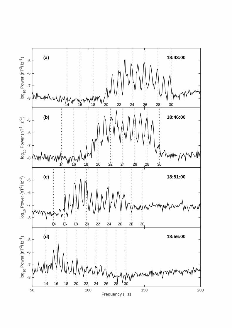
log

10 P

ower

(nT

2H

z-1)

-8

-7

-6

-5

14 16 18 20 22 24 26 28 30

18:43:00(a)

log

10 P

ower

(nT

2H

z-1)

-8

-7

-6

-5

14 16 18 20 22 24 26 28 30

18:46:00(b)

log

10 P

ower

(nT

2H

z-1)

-8

-7

-6

-5

14 16 18 20 22 24 26 28 30

18:51:00(c)

Frequency (Hz)50 100 150 200

log

10 P

ower

(nT

2H

z-1)

-8

-7

-6

-5

14 16 18 20 22 24 26 28 30

18:56:00(d)

Frequency (Hz)60 70 80 90 100 110 120 130 140 150 160

log

10 P

ower

(nT

2H

z-1)

-8

-7

-6

-5

14 15 16 17 18 19 20 21 22 23 24 25 26 27 28 29 30

18:49:00

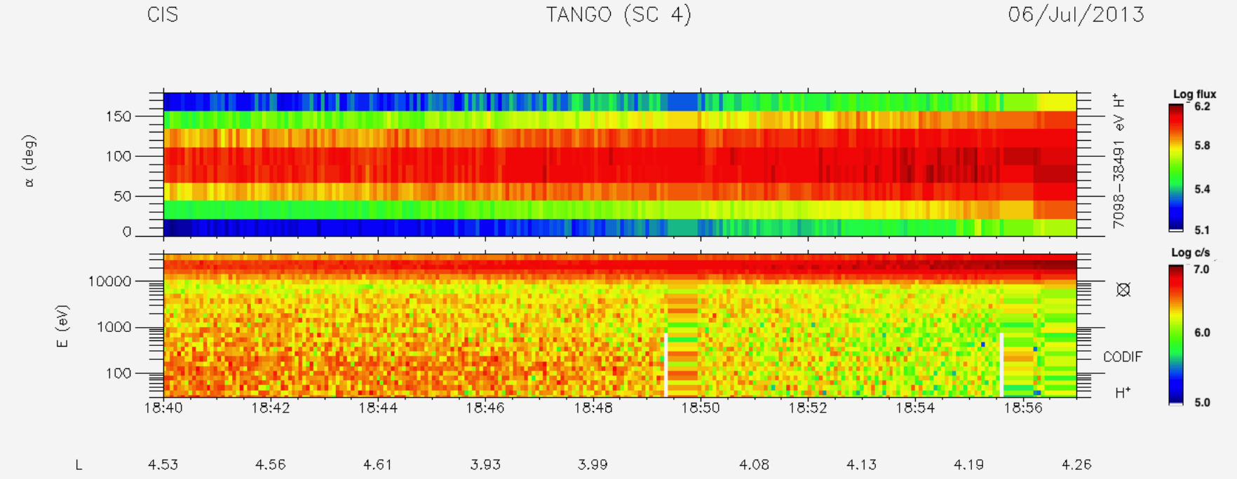
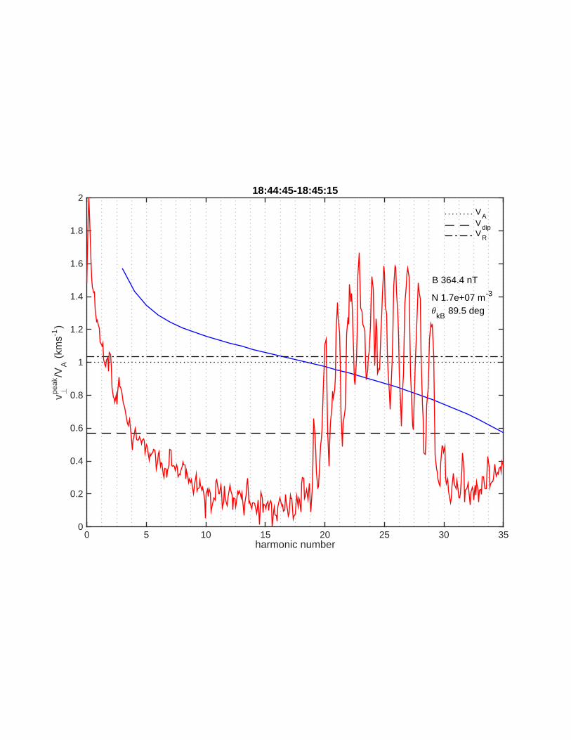
harmonic number0 5 10 15 20 25 30 35

v ?peak

/VA (

kms-1

)

0

0.2

0.4

0.6

0.8

1

1.2

1.4

1.6

1.8

2

B 364.4 nT

N 1.7e+07 m-3

3kB

89.5 deg

18:44:45-18:45:15

VAVdipVR

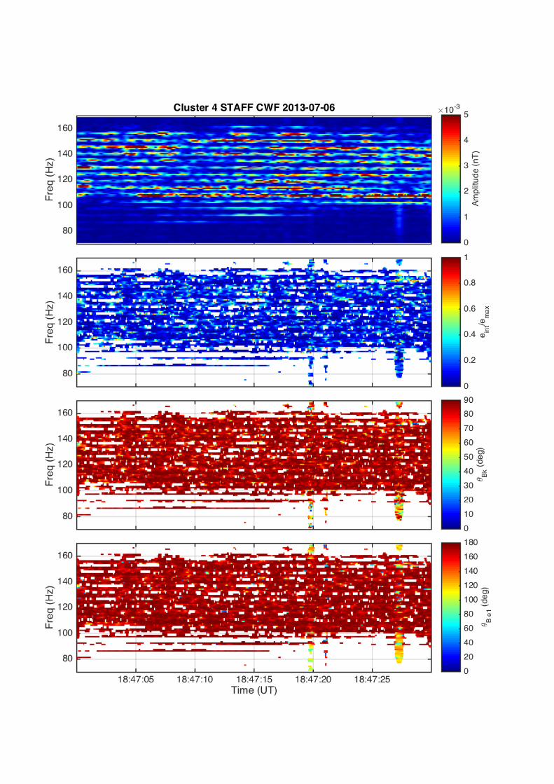
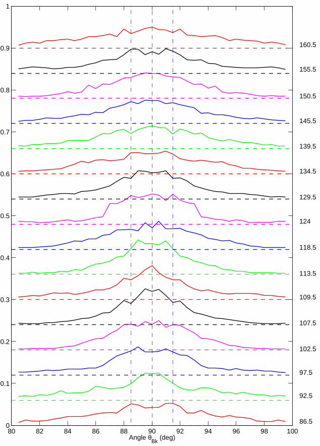
80 82 84 86 88 90 92 94 96 98 1000

0.1

0.2

0.3

0.4

0.5

0.6

0.7

0.8

0.9

1

86.5

92.5

97.5

102.5

107.5

109.5

113.5

118.5

124

129.5

134.5

139.5

145.5

150.5

155.5

160.5

Angle θBk

(deg)

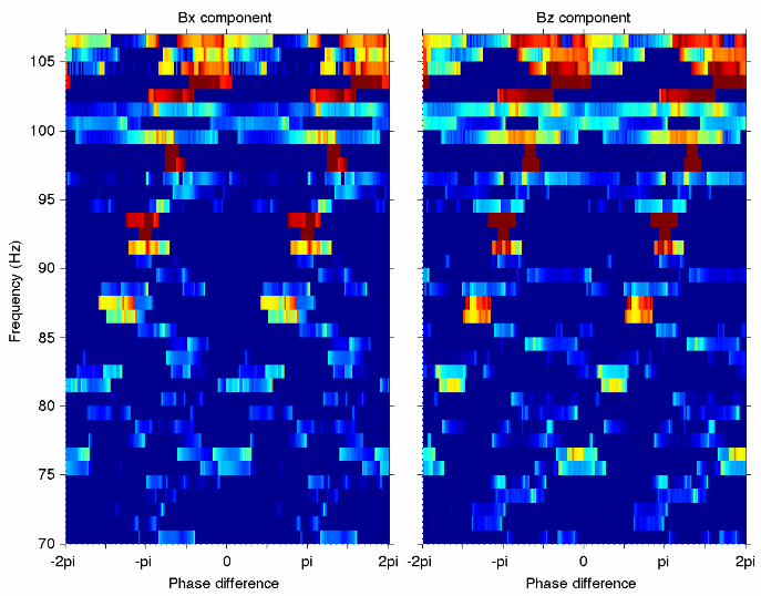
Normalized perpendicular component of the wave vector

Norm

aliz

ed p

ara

llel com

ponent of th

e w

ave v

ecto

rContours of constant frequency

−1 −0.8 −0.6 −0.4 −0.2 0 0.2 0.4 0.6 0.8 1−1

−0.8

−0.6

−0.4

−0.2

0

0.2

0.4

0.6

0.8

1

0 0.5 1 1.5 2 2.5 3 3.5 4 4.5 5−2

−1.5

−1

−0.5

0

0.5

1

1.5

2

2

3

L=4

Trajectory of the wave

X (Re)

Z (

Re)

kc/wpe

0.15 0.2 0.25 0.3 0.35 0.4 0.45 0.5 0.55

Fre

quen

cy (

Hz)

60

65

70

75

80

85

90

95

100

105

110

density 19 cm-3

density 15 cm-3

BzBx

experimental determination of the dispersion - spiral: home · 1 experimental determination of the...

Documents