experimental evaluation of a honeycomb structure in open
TRANSCRIPT

Scholars' Mine Scholars' Mine
Masters Theses Student Theses and Dissertations
Summer 2020
Experimental evaluation of a honeycomb structure in open Experimental evaluation of a honeycomb structure in open
channel flows channel flows
Kyle David Hix
Follow this and additional works at: https://scholarsmine.mst.edu/masters_theses
Part of the Hydraulic Engineering Commons
Department: Department:
Recommended Citation Recommended Citation Hix, Kyle David, "Experimental evaluation of a honeycomb structure in open channel flows" (2020). Masters Theses. 7952. https://scholarsmine.mst.edu/masters_theses/7952
This thesis is brought to you by Scholars' Mine, a service of the Missouri S&T Library and Learning Resources. This work is protected by U. S. Copyright Law. Unauthorized use including reproduction for redistribution requires the permission of the copyright holder. For more information, please contact [email protected].

EXPERIMENTAL EVALUATION OF A HONEYCOMB STRUCTURE IN OPEN
CHANNEL FLOWS
by
KYLE DAVID HIX
A THESIS
Presented to the Graduate Faculty of the
MISSOURI UNIVERSITY OF SCIENCE AND TECHNOLOGY
In Partial Fulfillment of the Requirements for the Degree
MASTER OF SCIENCE IN CIVIL ENGINEERING
2020
Approved by:
Cesar Mendoza, Advisor Robert Holmes Katherine Grote

© 2020
Kyle David Hix
All Rights Reserved

ABSTRACT
iii
Designing and controlling open channel flows presents many challenges. One
such challenge is energy dissipation. This challenge is currently addressed by several
means, including the use of honeycomb structures. Energy dissipation by honeycomb
structures has been studied for pressurized conduit flows; however, their ability to
dissipate energy in free-surface flows remains largely unexamined. This work introduces
a comprehensive experimental study designed to estimate the energy dissipation through
a honeycomb structure in a free-surface flow.
This work examined the energy dissipation for a range of flows, pipe lengths, and
pipe diameters in two flumes. PVC pipes ranging from 6 inches to 2 feet in length and
from / inch to 2 inches in diameter were used to build honeycomb structures. These
structures were subjected to a range of flows between 0.053 cubic feet per second (cfs)
and 4.310 cfs.
A non-linear regression analysis was conducted using SPSS software on the
measured data to obtain an empirical dimensionless equation. This empirical equation
represents the head losses as a function of discharge and geometric parameters. The
parameters in the empirical equation were examined by a sensitivity analysis to determine
which parameters are most influential. The results of this work showed that head losses
are correlated negatively with the pipe diameter, and positively with the discharge and
pipe length.

iv
ACKNOWLEDGMENTS
I would like to thank my Creator for giving me the opportunity and ability to
complete this work. I would also like to thank my family and friends for their support and
love. I would like to thank my advisor, Dr. Cesar Mendoza for leading me in this pursuit.
I would also like to thank my advisory committee, Dr. Robert Holmes and Dr. Katherine
Grote, for their support. Finally, I would like to thank my friend Dr. Wesam Mohammed-
Ali for his continued encouragement and support.

v
TABLE OF CONTENTS
Page
ABSTRACT....................................................................................................................... iii
ACKNOWLEDGMENTS................................................................................................. iv
LIST OF ILLUSTRATIONS............................................................................................vii
LIST OF TABLES............................................................................................................. ix
SECTION
1. INTRODUCTION...................................................................................................... 1
1.1. GENERAL INTRODUCTION........................................................................... 1
1.2. PURPOSE AND SCOPE.................................................................................... 1
1.3. THESIS ORGANIZATION............................................................................... 2
2. LITERATURE REVIEW........................................................................................... 3
2.1. GENERAL INTRODUCTION........................................................................... 3
2.2. WIND TUNNEL RESEARCH........................................................................... 4
2.3. WATER TUNNEL RESEARCH....................................................................... 5
2.4. OPEN CHANNEL RESEARCH........................................................................ 6
3. THEORY BASE FOR MODEL................................................................................. 8
3.1. SPECIFIC ENERGY.......................................................................................... 8
3.2. MODELS CONSIDERED................................................................................ 10
3.2.1. Darcy-Weisbach Model...........................................................................10
3.2.2. FHWA Model..........................................................................................12
3.2.3. Wind Tunnel Model................................................................................ 13
3.3. DIMENSIONAL ANALYSIS 14

Vi
4. EXPERIMENTAL WORK...................................................................................... 17
4.1. GENERAL INTRODUCTION......................................................................... 17
4.2. EXPERIMENTAL WORK DETAILS............................................................. 17
4.2.1. Experimental Setup................................................................................. 18
4.2.2. Large Flume............................................................................................ 18
4.2.3. Small Flume............................................................................................ 19
4.2.4. Test Section.............................................................................................21
4.2.5. Test Model.............................................................................................. 21
4.2.6. FlowTracker............................................................................................23
4.2.7. The Measurement Procedures.................................................................24
4.2.8. Summary of Test Conditions.................................................................. 25
4.3. STATISTICAL ANALYSIS............................................................................ 29
4.4. EMPIRICAL MODEL DEVELOPMENT....................................................... 31
4.5. SENSITIVITY ANALYSIS............................................................................. 33
5. RESULTS AND DISCUSSION.............................................................................. 39
6. CONCLUSIONS AND RECOMMENDATIONS................................................... 47
BIBLIOGRAPHY............................................................................................................50
VITA 52

LIST OF ILLUSTRATIONS
vii
Page
Figure 2.1 Types of Honeycombs....................................................................................... 3
Figure 3.1 Honeycomb Face..............................................................................................11
Figure 3.2 Dimensional Analysis Parameters....................................................................14
Figure 4.1 The 70-Foot Flume Control Panel....................................................................19
Figure 4.2 Panoramic View of the 70-Foot Flume............................................................ 19
Figure 4.3 The 16-Foot Flume...........................................................................................20
Figure 4.4 The 70-Foot Flume Channel............................................................................ 22
Figure 4.5 The 16-Foot Flume Channel............................................................................ 22
Figure 4.6 Typical Honeycomb Model............................................................................. 23
Figure 4.7 FlowTracker2 Probe.........................................................................................24
Figure 4.8 SPSS Input Data Windows.............................................................................. 30
Figure 4.9 Plot of Experimental Values vs Model Values................................................ 33
Figure 4.10 The Sensitivity Analysis of the Empirical Model to L/D.............................. 35
Figure 4.11 The Sensitivity Analysis of the Empirical Model to w/D..............................36
Figure 4.12 The Sensitivity Analysis of the Empirical Model to y/D...............................37
Figure 4.13 The Sensitivity Analysis of the Empirical Model to FrD............................... 37
Figure 5.1 The Predictability of the Darcy-Weisbach Model........................................... 40
Figure 5.2 The Predictability of the FHWA Model.......................................................... 40
Figure 5.3 The Predictability of the Eckert Model............................................................42
Figure 5.4 The Predictability of the Empirical Model...................................................... 42

viii
1/2 5/2Figure 5.5 The Plot of hi/D vs Q/(g D ) for w/D = 1...................................................43
1/2 5/2Figure 5.6 The Plot of hi/D vs Q/(g D ) for w/D = 1-1/3.............................................. 44
1/2 5/2Figure 5.7 The Plot of hi/D vs Q/(g D ) for w/D = 1-1/2.............................................. 44
1/2 5/2Figure 5.8 The Plot of hi/D vs Q/(g D ) for w/D = 2.....................................................45
1/2 5/2Figure 5.9 The Plot of hi/D vs Q/(g D ) for w/D = 2.4..................................................45
1/2 5/2Figure 5.10 The Plot of hi/D vs Q/(g D ) for w/D = 3.................................................46

ix
LIST OF TABLES
Page
Table 4.1 Test Conditions for 1 Inch Pipe Honeycombs...................................................26
Table 4.2 Test Conditions for 1-1/4 Inch Pipe Honeycombs............................................ 27
Table 4.3 Test Conditions for 2 Inch Pipe Honeycombs...................................................27
Table 4.4 Test Conditions for 3/4 Inch Pipe Honeycombs............................................... 28
Table 4.5 Test Conditions for 1/2 Inch Pipe Honeycombs............................................... 29
Table 4.6 SPSS Parameter Estimates................................................................................ 31
Table 4.7 Empirical Model Performance.......................................................................... 32
Table 4.8 Model Performance Comparison.......................................................................32
Table 4.9 Summary of Sensitivity Analysis...................................................................... 34
Table 4.10 Sensitivity Analysis Results............................................................................ 38
Table 5.1 Model Performance........................................................................................... 41

1. INTRODUCTION
1.1. GENERAL INTRODUCTION
Many solutions have been suggested and studied for the problem of energy
dissipation in open channel flows; one proposed solution is the use of honeycomb
structures. The honeycomb structure is an array of stacked up parallel conduits. The
energy dissipation phenomenon in a honeycomb has been studied for conduit pressurized
flows. However, the energy dissipation in free-surface flows remains largely
unexamined.
1.2. PURPOSE AND SCOPE
The purpose of this study is to investigate the head loss through a honeycomb
structure in open-channel and provide a design procedure for honeycomb structures for
use in an open channel. This was accomplished by reviewing literature related to
honeycomb flow conditioner design, determining dimensionless parameters effecting
head loss, collecting experimental data and developing an empirical model from a
statistical analysis of the experimental data. The empirical model was compared to
theoretical models to demonstrate the value of the empirical model. The impact of each
parameter was plotted to develop design charts. Additionally, a sensitivity analysis was
performed to identify the most influential parameter. The results of the empirical model
development and sensitivity analysis were used to develop a design procedure for
honeycomb structures.

2
1.3. THESIS ORGANIZATION
This thesis consists of six Sections. Section 1 contains the general introduction
and motivation of this work. Section 2 contains the literature review related to
honeycomb flow conditioner design, head loss through honeycombs, and other open
channel flow works. Section 3 contains the theory base for the model as well as the
theoretical models compared. Section 4 describes the experimental work including design
of the experiments, data collection, data analysis, empirical model development,
sensitivity analysis and comparison to theoretical models. Section 5 contains the results
and discussion of the work. Finally, Section 6 describes the conclusions and
recommendations from the study.

3
2. LITERATURE REVIEW
2.1. GENERAL INTRODUCTION
Flow conditioning is necessary for many applications. Whether it be discharge
measurement or component testing, having a predictable flow is critical for confidence in
the results. Flow conditioning has been studied in many applications. Much of those
studies have been in wind and water tunnel applications and there is some design
guidance. However, in open channels, flow conditioning relies on channel length or “rule
of thumb” conditioners. This outline defines the terms “flow conditioning” and
“honeycomb.” It gives a brief overview of relevant studies in wind and water tunnels as
well as research in open channel flows. It also shows the lack of research on honeycomb
structures for open channel flow conditioning.
Flow conditioning defines the techniques implemented to produce a known and
repeatable velocity profile. Many techniques are currently used. Screens, orifice plates,
vanes, approach sections and honeycombs. Prandtl [1] defined honeycombs as “a guiding
device through which the individual air filaments are rendered parallel”. This definition
applies to water “filaments.” By this definition, honeycombs are flow conditioners.
Honeycombs can come in multiple shapes as shown in Figure 2.1 [2].
Figure 2.1 Types of Honeycombs [2],

4
2.2. WIND TUNNEL RESEARCH
Most research on honeycombs has focused on wind tunnel applications. The
research ranges from design principles based on experience to turbulence reduction
studies. Prandtl [1] described honeycombs and discussed their application principles to
wind tunnels. Prandtl recommended depth to division (length to diameter) ratios between
4 and 7and emphasized the importance of the parallel components in the honeycomb. He
further suggested different locations for the honeycomb structure depending on the type
of air stream desired and the method employed to produce it. Prandtl’s design guidance is
based on years of experience in conducting wind tunnel testing. Barlow et al. [2] in more
recent design guidance agrees with Prandtl suggesting typical depth to division ratios
from 6-8.
Wind tunnel research has evaluated the performance of flow conditioners and
provided empirical theories to predict the performance. Scheiman and Brooks [3] noted
that empirical theories for performance correlated well with the given experimental data
but were unable to consistently predict the performance of a given structure.
The wind tunnel literature on the pressure drop through honeycombs introduced
some empirical solutions in terms of the pressure-loss coefficient. The Eckert Equation,
as given represented in (1), is one such empirical equations to predict the pressure-loss
coefficient. It is reproduced here in the form adopted by Barlow et al. [2]:
K” = A” ( # ; + 3 )(%;) + (%;- 1 ) (1)
where Dh is the hydraulic diameter of the honeycomb cell, Ph is the honeycomb porosity
and Lh is the thickness of the honeycomb in the direction of flow,

5
=
fo . 3 7 5
I 0 . 2 1 4
,0 .4
<Dh ,
0 -2 1 4 ( # ; )
( D ) ReO1 forR+A < 2750.4
eA ^
for ReA > 275(2)
where ReA is the Reynolds number based on material roughness and incoming flow speed,
and A is the surface roughness in the honeycomb cells. According to Idelcik, Eckert’s
equation is a simplification of an equation for pressure losses in radiators developed from
experimental data [4].
The empirical nature of honeycomb design and implementation and the
performance prediction emphasizes the complexity of the problem. Available design
guidance relies on rules of thumb and best practices. Additionally, it is abundantly clear
from Barlow et al. [2], Scheiman and Brooks [3] and Idelcik [4] that the performance of
flow conditioners is difficult to predict and their design follows best practice guidelines .
2.3. WATER TUNNEL RESEARCH
Standard wind tunnel turbulence reduction practice has been translated to water
tunnels, but Lumley [5] maintained that those standards can be unacceptable in large
water tunnels. Lumley and McMahon [6] reported that the standard wind tunnel practice
of using screens was found to be unsuitable due to “singing” effects during vortex
shedding in the Garfield Thomas Water Tunnel at the Ordinance Research Laboratory
and honeycombs were implemented instead. The effectiveness of honeycombs in water
tunnels motivated the studies in Lumley [5] and Lumley and McMahon [6]. These studies
centered on the reduction of turbulence intensity immediately downstream of the
honeycomb by using Batchelor’s approach. This analysis produced design charts for
honeycombs in water tunnels if certain parameters are known. These charts provide a

means to design if the turbulence is known. They can be used to estimate the pressure
drop coefficient if the ratio of the integral scale of the oncoming turbulence to the cell
depth as well as the ratio of final to initial turbulence levels are known. They also can be
used to find the pressure drop coefficient if the length to diameter ratio, constant length
Reynolds number, and diameter Reynolds are known. The analysis of the collected
experimental data provided “good quantitative support” and also showed the efficiency,
with respect to the pressure drop, when compared to data for a screen. Lumley found [5]
that the honeycomb required H the velocity head as that of the screens. Furthermore,
these studies introduced a procedure for selecting a turbulence-suppressing honeycomb
for application in a water tunnel. The research reported in Lumley [5] and Lumley and
McMahon [6] confirmed that honeycombs effectively reduce lateral turbulence but can
enhance turbulence as the flow in the components of the honeycomb becomes laminar.
The design process of a water tunnel including a honeycomb was described by
Jiang et al. [7]. The honeycomb design was selected based on the nature of the flow in the
components of the honeycomb, pressure loss and ease of construction. Although the
expected turbulence reduction is thoroughly considered, the pressure drop determination
is not mentioned. Water tunnel research begins to bridge the gap between the wind tunnel
research and the open channel flow applications.
2.4. OPEN CHANNEL RESEARCH
Flow conditioning in open channels has also received some attention. Most of this
research is focused on screens and screen-like structures. Yeh and Shrestha [8] were
motivated to study the flow through screens at different inclinations for use in fish
6

screens. They reported that there was an optimal inclination level to minimize the
magnitude of the head loss, but their measurements were slightly different than their
model predicted. They noted that transverse bars, an integral structural component of the
screen, was likely causing this discrepancy.
The work by Yeh and Shrestha [8] was the basis for the investigation conducted
by £akir [9]. £akir studied the energy dissipation potential of screens downstream of a
sluice gate. The work was limited to the supercritical flow expected to occur downstream
of hydraulic structures. In general, it was found that the performance of the screens
improved with increases of the Froude number and with a decrease in the ratio of the
distance to screen and the height of gate opening. The work added to the range of
experimental data on screens in open channels.
Another study on head losses through structures was conducted by Tsikata [10].
He studied the effect of bar and rack geometry on trash racks typically attached to
hydropower generating units. The work provides an in-depth analysis of the hydraulic
impacts of different trash rack configurations. The work showed that head loss was
positively correlated with the approach velocity as well as with the blockage ratio.
Additionally, for set bar spacing, the head loss is positively correlated with the bar
thickness. Streamlined and rounded bars reduced the head loss. The study provides
valuable information for designers and operators generating hydroelectric power plants.
The research work done in open channels covers a limited range of hydraulic
structures. Additionally, the work has produced important design guidance for the studied
structures. The research, however, has yet to evaluate honeycomb structures.
7

8
3. THEORY BASE FOR MODEL
3.1. SPECIFIC ENERGY
The energy equation provides a steady flow equation for frictionless flow. The
equation relates pressure, velocity, and elevation. The energy, referred to as head, the
sum of the pressure head, the velocity head, and the elevation head. The equation is used
to relate the energy of the flow in one location to another. The energy equation is
presented in Equation 3
Pi + v ? + = P# + x ! + Z2 + h f + hm (3). 2g 1 . 2g 2 f m W
where p is the pressure, y is the specific weight, V is the velocity, g is the gravitational
acceleration, z is the depth, hf is the friction head loss, and hm is the minor head loss.
On the downstream side of the equation the head loss terms are included. The
head loss in open channels can be simplified to two terms, friction loss and minor loss.
Friction losses are a result of the interaction of the fluid with the channel boundary. The
minor losses are a result of changes in the movement of the fluid, typically caused by
changes to channel geometry or obstructions in the channel. Many ways to predict the
friction loss have been developed and well tested. However, minor losses rely strongly on
experimental work.
Minor losses are typically given as a ratio of the head loss to the velocity head and
are determined using a loss coefficient [11]. The equation showing the relation of minor
losses to velocity head and the loss coefficient (K) as presented by White is reproduced in
Equation 4

9
(4)
where p is the density.
The energy equation can be simplified for open channel flows in the form of
specific energy [11]. The specific energy consists of the flow depth and the velocity head
and represents the height of the Energy Grade Line. The specific energy equation is
presented in Equation 5.
(5)
where y is the depth of flow and E is the specific energy.
The specific energy can be used to compare different energy values for the same
where h8 is the head loss.
This is done because the flumes are leveled, elevation upstream is equal to
elevation downstream. Additionally, friction losses from the channel can be neglected
since the measurements occur immediately upstream and downstream of the structure.
Since the velocity was not measured directly, rather the discharge was measured,
Equation 4 must be adjusted. The continuity equation relates the discharge, velocity and
area of flow. The continuity equation is presented in Equation 7
discharge rate. For this work the specific energy principle is used to measure the head
loss through the test section. The measured head loss is determined using Equation 6
(6)
Q = V * A (7)
where Q is the volumetric discharge and A is the flow area.

10
Combining Equations 6 and 7 results in the final form of the specific energy
equation for this work. This form was used to determine the head loss through the
honeycomb using the experimental measurements and is presented as Equation 8
y $ +9 "
2 g ( w c *y1) 2 y& +q 2
2g(W c*y2)2+ h i (8)
where wc is the width of the channel.
3.2. MODELS CONSIDERED
Three theoretical models were proposed to predict the head loss through the
honeycomb structure. The first, the Darcy-Weisbach model, predicts flow through a pipe.
The second, the FHWA culvert equation model, considers flow through a conduit that is
either full or partially full. The final, the Eckert Equation model, predicts the head loss
coefficient for honeycomb structures in wind tunnels. Each model was developed for
different uses but are applied here to examine their usefulness and to support the need for
developing an empirical model.
3.2.1. Darcy-Weisbach Model. The Darcy-Weisbach equation predicts the
friction head loss through a pipe by considering its length, its diameter, the dimensionless
friction factor, and the velocity head as seen in the form
@ B 2h f = f ~A 2g (9)
where f is the friction factor, L is the length of pipe, and d is the pipe diameter.
Equation 9 was applied to each pipe in the structure. The friction factor was
estimated from the Moody diagram based on the material characteristics and the

11
assumption of fully turbulent flow. As shown in Figure 3.1, due to the geometry of the
honeycomb structure, non-circular conduits exist.
White [11] provides a means of predicting the friction head loss by replacing the
diameter with the hydraulic diameter. The hydraulic diameter, Dh„ is estimated as
Dh = —n p ( 10)
where A is the cross-sectional area and P is the wetted perimeter.
Figure 3.1 Honeycomb Face.
The minor loss equation, Equation (4), was used to model the entrance and exit
losses for each conduit. Standard loss coefficients of 0.5 and 1 were used for the entrance
and exit, respectively. In order to apply the model to the experimental observations, some
simplifying assumptions were introduced. It was assumed that the average velocity of the
flow upstream of the structure is uniformly distributed across the face of the structure.
The irregular pipe sections along the boundary of the channel and the structure were not
modeled as it was assumed that losses through these channels comprised a negligible
portion of the total loss. The model was implemented by determining the head loss for

12
one representative pipe, both regular and irregular then multiplying that loss by the total
number of each pipe in the flow area. The head loss determined included the Darcy-
Weisbach friction head losses and the minor losses.
3.2.2. FHWA Model. The second model applied the FHWA culvert equations
for head loss. The outlet controlled full-flow head loss equation was applied to all pipes
but those in the top layer of pipes in the flow area. The full flow head loss equation is
calculated as
H = 1 + k e +Ku n 2L~l V#
R 133 J 2g (11)
where H is the barrel loss, ke is the entrance loss coefficient, Ku is a unit constant (29 in
English units), n is Manning’s roughness coefficient, and R is the hydraulic radius.
The outlet control partial flow head loss equation was applied to the top row of
pipes in the flow area. First, the criteria for partial flow, TW>D (TW is the tailwater
depth and D is the pipe diameter) , was confirmed by comparing the tailwater depth to
the diameter of the pipe. T
When using Equation (10), the tailwater depth was taken as the depth of flow
from the bottom of the pipe to the free surface on the downstream end of the pipe. Once
partial flow was confirmed, the critical depth for the pipe was determined. Following the
Texas DOT manual [12], the following three equations were solved iteratively to find the
critical depth.
(12)
where Ac is the area at critical depth and Tc is the top-width at critical depth,

13
A r = - [2cos 1 $1 - &#%'- sin $2cos 1 $1 - &#%))] (13)
where dc is the critical depth,
Tc = D sin (cos"1 (2O#=# )) (14)
Once the critical depth was determined for a given iteration, the head loss was
computed using the empirical formula given by Mays [13].
H = HW0 - h 0 (15)
where HW0 is the headwater depth above the outlet invert and h0 is determined from
[13].
h0 = max TW, (D + dcV 2] (16)
The full flow head loss and partial flow head loss were combined to determine the
total predicted head loss.
3.2.3. Wind Tunnel Model. The third model used the Eckert equation originally
developed from experimental data. This equation comes from wind tunnel research data
and predicts the loss coefficient for use in the minor loss equation, Equation (4).
K„ = * „ (# ! + 3' (/ ) 2 + ( $ - i )2 ( 17)
where Dh is the hydraulic diameter of the honeycomb cell, Ph is the honeycomb porosity
and Lh is the thickness of the honeycomb in the direction of flow,
A h
*
0 . 3 7 5 Gt ) 0 4 J 0 1 / o r ^ A < 2 7 5KDh J
0.214$—)\ D h J
0.4 (18)/o r ReA > 275
where ReA is the Reynolds number based on material roughness and incoming flow speed,
and A is the surface roughness in the honeycomb cells.
The parameters for the equation were determined for each test model and flow
regime. The predicted loss coefficient was used in combination with Equation (2) to
determine the predicted head loss.
3.3. DIMENSIONAL ANALYSIS
It is well stablished that dimensional analysis is an effective tool for simplifying
complex phenomenon and directing experimental data collection programs. Additionally,
dimensional analysis can simplify the experimental results to the point that they are easily
accessible [11, 14], A dimensional analysis was conducted to determine the effects of the
intervening parameters on the minor loss through the honeycomb structure. The results of
the dimensional analysis informed the experimental setup and the development of the
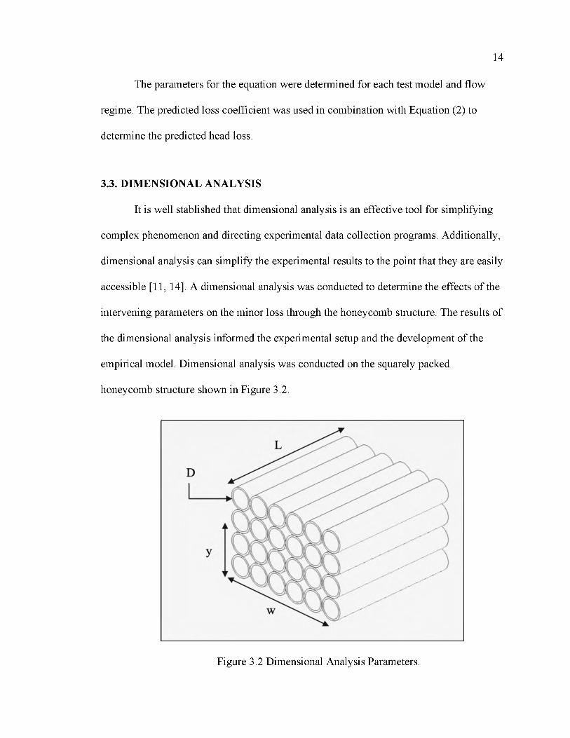
empirical model. Dimensional analysis was conducted on the squarely packed
honeycomb structure shown in Figure 3.2.
14
Figure 3.2 Dimensional Analysis Parameters.

15
The variables pertinent to head loss through the honeycomb were identified. The
geometric variables were the diameter of the pipes, D, the depth of the pipes, L, and the
width of the structure, w. The flow property variables were the discharge, Q, and the
height of the free surface, y. The fluid property variables were the mass density, p, the
dynamic viscosity, p, and the acceleration due to gravity, g.
The formula for head loss, h8, through the structure can be written as a function of
the intervening variables as
hi = f(D, L, w, y, Q, g, p, p) (20)
Then, the number of variables N is equal to 9
(hi, D, L, w, y, Q, g, p, p) = 0
The above parameters in dimensional form are, L,L,L,L,L, S , S#, , @S ,
(21)
therefore, the number of dimensions is three and the number of n groups is determined,
9-3 = 6. The primary variables are (p, g, D). Equation (21) c is now written as,
^2 (nl, n 2, n 3,n 4, n 5,n 6) = 0 (22)
/ Q^ 3 l 1 5
g2D2 pg2D2
w " ; = W = 0, " D( , D , D , D , D IPg2# 2
(23)
The term I -r-* I represents Froude’s Number, and will be called the DiameterC2D2
Froude Number (Fm), and the term I — I represents Reynolds Number (Re). EquationPC2D2
(23) can be rewritten as
(24)
Finally,

16
# = + u ( F r ° - R e - # ■ ; ■ # ) <25)
For this work, values for Re ranged from 4473 to 35784 which can be considered
fully turbulent [13]. Since the flow is turbulent, the Reynolds number parameter was
dropped from Equation (25) and the simplified functional equation became
# = « ■ ( F r # . # ■ ; . # ) (26)
Equation (26) is the foundation of the empirical model.

17
4. EXPERIMENTAL WORK
4.1. GENERAL INTRODUCTION
In this section, the experimental facilities, equipment, measuring techniques,
conditions and procedures are described. The experimental results and analysis of the
data is also presented. Finally, the development of the empirical model is introduced.
The experiments were conducted on two scales with a range of pipe diameters and
lengths. The ranges of the experimental work were selected to evaluate the parameters
identified in the dimensional analysis. Details about the experimental work including
setup, facilities, equipment, and models are described in Section 4.2. The experimental
setup is described in Section 4.2.1. Sections 4.2.2 and 4.2.3 describe the two flumes used
in the tests. The test section and test models are described in Sections 4.2.4 and 4.2.5.
Section 4.2.6 and 4.2.7 describe the measurement equipment and procedure respectively.
Finally, Section 4.2.8 summarizes the test conditions for each series of parameters.
The results of the experimental work were subjected to statistical analysis. The
statistical analysis is described in Section 4.3. The outcome of the statistical analysis was
the empirical model developed for the conditions of the experiment. The model is
discussed in Section 4.4.
4.2. EXPERIMENTAL WORK DETAILS
The experimental work details are included in sections 4.2.1 to 4.2.9. Each section
describes one aspect of the experimental work.

18
4.2.1. Experimental Setup. The experiments were conducted in two flumes at
the Missouri University of Science and Technology Hydraulics Lab. The tests were
separated into series depending on the pipe diameter and were conducted for a range of
dimensionless parameters. The w/D values ranged from 1 to 3, the L/D values ranged 0.5
to 2.67, the y/D values ranged from 1 to 5. Finally, the pipes were tested at a range of
discharges from 0.053 to 4.310 cubic feet per second (cfs). Tests on honeycomb
structures built with 1”, 1.25” and 2” diameter pipes were conducted in the 70-foot flume.
Tests on honeycomb structures built with 1”, %” and / ” in diameter pipes were
conducted in the 16-foot flume. Discharges were measured directly with a SonTek
Flowtracker in the 70-foot flume and with built in orifice meters in the 16-foot flume.
The depth of flow was measured upstream and downstream of the honeycomb structure.
The results of the experimental observations were used to develop the empirical equation.
4.2.2. Large Flume. The large flume in the hydraulics lab was used for large
diameter pipes. The flume is 70 feet long, 3 feet deep and 3 feet wide. The channel is
constructed of clear acrylic sides and had a cement false bottom. The flume is supported
by a steel frame. The flume slope can be changed by varying the elevation of the flume
upstream end. For these experiments conducted for this work, the flume was maintained
at a horizontal grade. The flume was serviced by 4 pumps; two large and two small. The
large pumps are driven by MagnaTek D-390821-02 100 hp motors. The small pumps are
driven by MagnaTek 7-860099-01-OJ 16 hp motor. The large pumps a Bell & Gossett 6G
12.250 BF pumps. They can produce 1250 gallons per minute (gpm) and 150 ft of head.
The small pumps are Bell & Gossett 3B 9.125 BF pumps. They can produce 400 gpm and
75 ft of head. The pumps are controlled using InTouch WindowViewer software. The

control panel allows the user to select pumps to use and then determine the pump speed
of the pumps. The control panel is presented in Figure 4.1. In this work, the two large
pumps were both used. A panoramic view of the 70-ft long flume is shown in Figure 4.2.
19
Figure 4.1 The 70-Foot Flume Control Panel.
Figure 4.2 Panoramic View of the 70-Foot Flume.
4.2.3. Small Flume. The small flume in the hydraulics lab was used for testing
honeycomb structures made with small diameter pipes.
The flume is a model B-16 Hydraulic Demonstration Channel, designed and built
by Engineering Laboratory Design Inc. The flume channel is 16 feet long, 1 foot wide,
and 1.5 feet deep. The channel is constructed of 0.5 in thick clear acrylic. Figure 4.3
shows the 16 ft flume.

20
Figure 4.3 The 16-Foot Flume.
The flume reservoir, which holds approximately 136 gallons of water, serves the
two flume pumps. The pumps are low head, high volume pumps (Price Pump Model
XT200AB-525-21m-75-18C-1D6) and are powered by Baldor Model No.
34F181W198 motors. Each pump delivers 95 gallons per minute (gpm) at 25 feet of head
for a maximum total flow of 190 gpm. Two orifice flow meters are available for flow
discharge measurements. The orifice flow meters are read using a U-tube manometer and
a calibration curve. The calibration equation for the small orifice flow meter in (ft3/s) is
Q = 0.0554 * VAh(ft) (27)
where Ah is the manometric reading height in feet. The calibration equation for the large
orifice flow meter in (ft3/s) is
Q = 0.2009 * VAh(ft) (28)
The calibration equations were used to determine the discharge during the small-
flume experiments. The flume utilizes a headtank to reduce turbulence from the pumps.

The headtank has a headgate to control the pressure of the flow in the flume. The
headgate was raised so it had no effect on the experiments. The flume also has a tailgate
for flow depth control. The flume was leveled, and the tailgate lowered parallel to the
channel bed for the testing.
4.2.4. Test Section. The test section was located near the middle of each flume.
This provided significant distance downstream from the stilling basin for the flow to be
uniform and fully developed. The test section materials were consistent with the rest of
the flume channel. In the 70-Foot flume the side walls were clear acrylic and the bed
cement. In 16-Foot flume all bounding sides were clear acrylic. The cross-sectional area
of the test section was rectangular uniform with the rest of the channel geometry as well.
For models that didn’t fit flush with the side walls spacers were used to close the gap on
one side. The spacers forced the flow to go through the structure so head loss could be
attributed to the structure itself. The models were assembled in the test section and
altered as needed. The models were aligned parallel to the direction of flow within the
test section. Models were secured by setting small steel beams or plates on top of the
structure. Typical channel sections, representative of the test sections, are shown in
Figures 4.4 and 4.5.
4.2.5. Test Model. The test models consisted of readily available PVC pipes cut
to length and assembled as a squarely stacked honeycomb. Five pipe diameters were
tested: / ”, %”, 1”, 1-1/4” and 2” (NPS) notation. The pipes were cut to 2 feet in length, 1
foot in length and 0.5 feet in length. These lengths provided L/D ratios of 0.5 to 2.67.
The pipes were stacked vertically on center. For each honeycomb structure, the
pipes were secured using static friction aided with weight distributed along the top of the
21

22
structure. The weight was in the form of two, 3-foot long steel I-beams or four steel
plates stored in the lab. The honeycomb was oriented so that the pipes were parallel to the
channel. A typical non-staggered honeycomb assembly can be seen in Figure 4.6.
Figure 4.4 The 70-Foot Flume Channel.
Figure 4.5 The 16-Foot Flume Channel

23
Figure 4.6 Typical Honeycomb Model.
4.2.6. FlowTracker. The SonTek FlowTracker is an acoustic doppler velocimeter
( A D V ) . It utilizes Doppler shift to measure the velocity of the flow. The Doppler
principle states that the frequency of the sound transmitted to a receiver shifts if the
source of the sound is moving relative to the receiver.
Fd o p p le r = Fsource * (29)
where, F d o PPier is the Doppler shift, F S0Urce is the transmitted frequency, V is the velocity of
the source relative to the receiver, and C is the speed of sound. The FlowTracker is a bi
static Doppler current meter which means the transmitter and receiver are located on the
same probe. The receivers are mounted such that sampling beams intersect in a volume of
water 4 in from the tip of the probe. The transmitted acoustic beam is reflected by
particles in the water and the modified frequency is sampled by the receivers. The
Doppler shift is used to determine the velocity using Equation (29). The probe alignment
can be seen in Figure 4.7.

24
Cylindrical Sampling Volume Fixed Distance to6 mm Diameter Remote Sampling Volume9 mm Height 10 cm (nominal)
Figure 4.7 FlowTracker2 Probe.
The FlowTracker can measure velocities in the range between 0.003 and 13 feet
per second (ft/s) with accuracies up to 1% of measured velocity for each one-second
sample. These characteristics made this instrument well suited for the large-flume
experiments where the expected velocities were less than 4 ft/s. It is assumed that the
velocity of the particles represents the velocity of the water itself. The FlowTracker
automatically calculates the discharge using the Mid-Section, Mean-Section, or the
Japanese Equation method. For the large scale experiments the Mid-section method was
selected. The mean velocity was sampled at 0.6 of the flow depth. Since the channel was
uniform and rectangular, only one measurement was made at mid-channel.
4.2.7. The Measurement Procedures. Although the measurement procedures for
the large-scale and the small-scale tests were similar, some differences worth reporting
were also implemented. In the large-scale tests the discharge was adjusted using the
flume control software to change the pump speed. Discharge was set such that the flow
depth at the upstream end of the structure was flush with the top of a given row in the
structure. The flow was given ample time to stabilize at each depth. The SonTek

FlowTracker2 was used to obtain the discharge. The measurement was taken in the
middle of the channel at a location approximately 12-12.5 feet upstream of the structure.
Once the discharge was measured, the upstream and downstream depth were measured
on each side of the flume. Five sets of depth measurements were taken. The depth was
recorded using a scale fixed to the exterior face of the flume. The depth was measured
from the bed to the free surface. The downstream flow depth was measured at the vena
contracta in the downstream discharge using a non-fixed scale. The averaged depths were
used in the calculation of head loss. After the depths were measured the discharge was
adjusted and the process repeated.
In the small-scale experiments the discharge was adjusted using the gate valves
near the upstream end of the flume. The discharge was set such that the flow depth at the
upstream end of the structure was flush with the top of a given row in the honeycomb
structure. The flow was given ample time to stabilize at each depth. The orifice meters
were read and recorded. Once the discharge was measured, the upstream and downstream
depth was measured on either side of the flume. Five sets of depth measurements were
taken. The depth was recorded using a Vernier Scale. The depth to the bed was measured
and then the depth to the free surface. The difference in the two measurements
represented the flow depth. The downstream depth was measured at the vena contracta in
the downstream discharge following the same method as upstream. After the depths were
measured the discharge was adjusted and the process repeated.
4.2.8. Summary of Test Conditions. The test conditions for each series of tests
are summarized in Tables 4.1- 4.5. The water properties and environmental conditions
were kept constant throughout the experimental work. The series were separated by pipe
25

diameter and summarized below. The width and length units for the parameters were in
feet while the flow depth and diameter units were in inches. The discharge units were
cubic feet per second.
The 1 Inch pipe was tested in 12 separate scenarios. The pipes were tested in both
the small flume and the large flume resulting in w/D values of 2 and 3. The pipes were
also tested at two lengths resulting in L/D values of 1 and 2. The pipes were tested at
multiple y/D values, depending on the test flume used, resulting in a range from 1 to 5.
Finally, the pipes were tested at a range of discharges from 0.093 to 2.662 cubic feet per
second (cfs). The summary of the 1 Inch Pipe tests is given in Table 4.1.
26
Table 4.1 Test Conditions for 1 Inch Pipe Honeycombs.
Test Q (cfs) L/D w/D y/D hL
D=1 (1) 0.093 1 1 1 0.014
D=1 (2) 0.251 1 1 2 0.037
D=1 (3) 0.428 1 1 3 0.047
D=1 (4) 0.064 2 1 1 0.018
D=1 (5) 0.226 2 1 2 0.042
D=1 (6) 0.415 2 1 3 0.069
D=1 (7) 1.099 1 3 3 0.068
D=1 (8) 1.927 1 3 4 0.093
D=1 (9) 2.662 1 3 5 0.106
D=1 (10) 1.077 2 3 3 0.084
D=1 (11) 2.003 2 3 4 0.111
D=1 (12) 2.662 2 3 5 0.123

27
The 1-1/4 Inch pipe was tested in 6 separate scenarios. The pipes were tested in
the large flume resulting in a w/D value of 2.4. The pipes were tested at two lengths
resulting in L/D values of 1.6 and 0.8. The pipes were tested at y/D values in the range
between 2 and 4. Finally, the pipes were tested at a range of discharges from 1.227 to
3.914 cfs. The summary of the 1-1/4 Inch Pipe tests is given in Table 4.2.
Table 4.2 Test Conditions for 1-1/4 Inch Pipe Honeycombs.
Test Q (cfs) L/D w/D y/D hLD=1.25 (1) 1.227 1.6 2.4 2 0.055D=1.25 (2) 2.330 1.6 2.4 3 0.072D=1.25 (3) 3.177 1.6 2.4 4 0.075D=1.25 (4) 1.246 0.8 2.4 2 0.060D=1.25 (5) 2.396 0.8 2.4 3 0.101D=1.25 (6) 3.914 0.8 2.4 4 0.101
The 2 Inch pipe was tested in 6 separate scenarios. The pipes were tested in the
large flume resulting in a w/D value of 1.5. The pipes were tested at two lengths resulting
in L/D values of 1 and 0.5. The pipes were tested for y/D values in the range from 1 to 3.
Finally, the pipes were tested in the range of discharges from 0.572 to a 4.31 cfs. The
summary of the 2 Inch Pipe tests is presented in Table 4.3.
Table 4.3 Test Conditions for 2 Inch Pipe Honeycombs.
Test Q (cfs) L/D w/D y/D hLD=2 (1) 0.573 1 1.5 1 0.044D=2 (2) 1.213 1 1.5 2 0.111D=2 (3) 3.720 1 1.5 3 0.115D=2 (4) 0.572 0.5 1.5 1 0.045D=2 (5) 2.322 0.5 1.5 2 0.057D=2 (6) 4.310 0.5 1.5 3 0.079

28
Nine separate test were conducted with the 3/4-inch pipe. These pipes were tested
in the small flume resulting in a w/D value of 1.33. The pipes were tested at three lengths
resulting in L/D values of 2.67, 1.33, and 0.67. The pipes were tested in a range of y/D
from 2 to 4. Finally, the pipes were tested in a range of discharges between 0.120 and
0.379 cfs. The summary of the 3/4 Inch Pipe tests is presented in Table 4.4.
Table 4.4 Test Conditions for 3/4 Inch Pipe Honeycombs.
Test Q (cfs) L/D w/D y/D hL
D=3/4 (1) 0.334 2.67 1.33 4 0.119
D=3/4 (2) 0.224 2.67 1.33 3 0.084
D=3/4 (3) 0.125 2.67 1.33 2 0.047
D=3/4 (4) 0.379 1.33 1.33 4 0.093
D=3/4 (5) 0.252 1.33 1.33 3 0.071
D=3/4 (6) 0.120 1.33 1.33 2 0.043
D=3/4 (7) 0.365 0.67 1.33 4 0.078
D=3/4 (8) 0.260 0.67 1.33 3 0.064
D=3/4 (9) 0.136 0.67 1.33 2 0.040
The 1/2 Inch pipe was tested in 9 separate scenarios. The pipes were tested in the
small flume; the w/D ratio has a value of 2. The pipes were tested at three lengths
resulting in L/D values of 4, 2, and 1. The pipes were tested at y/D values in the range
from 2 to 4. Finally, the pipes were tested in a range of discharges from 0.053 to 0.284
cfs. The summary of the 1/2 Inch Pipe tests is presented in Table 4.5.

29
Table 4.5 Test Conditions for 1/2 Inch Pipe Honeycombs.
Test Q (cfs) L/D w/D y/D hL
D=1/2 (1) 0.226 4 2 4 0.114
D=1/2 (2) 0.130 4 2 3 0.076
D=1/2 (3) 0.053 4 2 2 0.042
D=1/2 (4) 0.254 2 2 4 0.084
D=1/2 (5) 0.157 2 2 3 0.061
D=1/2 (6) 0.073 2 2 2 0.032
D=1/2 (7) 0.284 1 2 4 0.069
D=1/2 (8) 0.180 1 2 3 0.056
D=1/2 (9) 0.076 1 2 2 0.027
4.3. STATISTICAL ANALYSIS
A non-linear regression of the experimental data collected was conducted using
the IBM software SPSS Statistics to determine an empirical model equation in line with
the functional equation derived by dimensional analysis. The general form of the
empirical model is
□ = x> (s)* # * xm (; r * x= sr * xa(pr” <3'
where the coefficients x1 through x8 are constants to be determined from the non-linear
regression, R is the ratio of the head loss in feet to the pipe diameter in inches, , FrD is
the Diameter Froude Number, R is the ratio of the depth of pipe in feet to the pipe
diameter in inches, R is the ratio of the structure width in feet to the pipe diameter in

30
•yinches, and - is the ratio of the free-surface height in inches to the pipe diameter in
inches. The experimental observations were randomized and split into two groups. The
data were assigned random numbers and then ordered from smallest to largest. The first
group was used in the regression analysis to determine the coefficients and represented
the first 3/4ths of the randomized data. The second group was used for validation of the
model and represented the remaining l/4th of the randomized data. Figure 4.8 shows the
SPSS input and Table 4.6 summarizes the values of the calculated parameters.
• 0 • Nonlinear Regression
£ LD $ wD /yD / F r
Parameters..
Xl(l)X2(l)X3(l)X4(l)X5(l)X6(l)X7(l)X8(l)
*
*
Dependent:/ h IDModel Expression:(X1*LD ** X2)*(X3*wD ** X4)*(X5*yD ** X6)*(X7*Fr ** X8)
tFunction group:
Loss...
Constraints..
Save-
Options...
± < > 7 8 9 AllArithmetic
□ <= 4 5 6 CDF & Noncentral CDF Conversion
* I - 1 ~= 1 2 3 Current Date/Time Date Arithmetic
/ & 1 0 n Date CreationDate Extraction
**~ 0 Delete Functions and Special Variables
Reset Paste Cancel OK
Figure 4.8 SPSS Input Data Windows.

31
Table 4.6 SPSS Parameter Estimates.
Parameter Estimate
X1 0.70
X2 0.49
X3 0.53
X4 -0.23
X5 0.32
X6 1.04
X7 0.24
X8 0.06
4.4. EMPIRICAL MODEL DEVELOPMENT
The empirical model equation was developed from the statistical analysis. Thus,
Equation (4) is now written as
0.49 —0.23 1.04# = ° .° 2 9 fe) y © Fr# (3»
The performance of the empirical model was evaluated using the Nash-Sutcliffe
model efficiency coefficient, NSE [15]
Xt(O-S)2NSE = 1 - Xt(O-O)#
where O is the observed variable, S is the simulated variable and 0 is the average of the
(32)
observed variable.

The NSE was chosen because it evaluates how well a model predicts observed
values in a stablished timescale. The timescale is the series of measurements for the
empirical model. The NSE is often used to gauge the efficiency of hydrologic models,
e.g. Mohammed-Ali et al. [16, 17]. An NSE value of 1 represents a model that perfectly
predicts the observed condition. A value of zero means the model will predict the mean
value of the observed events. Negative values represent models that don’t predict better
than the mean value. The numerical value of the parameters was obtained from the
statistical analysis and then the NSE was computed for the validation portion of the data.
Additionally, the NSE was computed for the model development portion of the data. The
model performance parameters are summarized in Table 4.7.
32
Table 4.7 Empirical Model Performance.
Parameters Development Validation
NSE 0.83 0.75
The model performance parameters for the considered models is summarized in
Table 4.8.
Table 4.8 Model Performance Comparison.
Model NSE
Empirical 0.75
Darcy -72939
FHWA -53526
Eckert -16.2

33
Figure 4.9 shows the plot of the experimental dimensionless head loss to modeled
head loss. The performance of the empirical derived model was compared with the results
of the other models considered. The empirical model performed the best out of the
models considered.
Experimental vs Model
h|/D (Empirical)
Figure 4.9 Plot of Experimental Values vs Model Values.
4.5. SENSITIVITY ANALYSIS
A sensitivity analysis was conducted to determine the effect of the variability of
the model parameter values on the magnitude of the estimated head loss values. The
purpose of the sensitivity analysis was to identify which parameters have the greatest
impact on head loss to inform future work with the empirical model. The parameter with
the greatest impact can be properly emphasized when designing future honeycomb
structures.

The sensitivity analysis was conducted on the empirical model by adjusting the
values of each parameter. Each parameter was increased and decreased by 10% and 30%
from the mean value in the experimental data. The parameters evaluated were L/D, w/D,
y/D and FrD as defined by the model. Table 4.1 contains a summary of the sensitivity
analysis.
34
Table 4.9 Summary of Sensitivity Analysis.
Test Description
1 L/D decreased by 30%
2 L/D decreased by 10%
3 L/D increased by 10%
4 L/D increased by 30%
5 w/D decreased by 30%
6 w/D decreased by 10%
7 w/D increased by 10%
8 w/D increased by 30%
9 y/D decreased by 30%
10 y/D decreased by 10%
11 y/D increased by 10%
12 y/D increased by 30%
13 FrD decreased by 30%
14 FrD decreased by 10%
15 FrD increased by 10%
16 FrD increased by 30%
The results of the sensitivity analysis revealed that the model was most sensitive
to the variations of the parameter y/D and least sensitive to variation of the parameters
w/D and Fr.

35
Figure 4.10 shows the results of the sensitivity analysis of the empirical model to
the parameter L/D. This figure suggests that increasing the length or decreasing the
diameter 10% results in an increase in dimensionless head loss of about 5% and that the
impact in percent change is about half that of the change in the parameter.
20 .0%
Sensitivity to L/D
15.0%
10.0%
^ 5.0%
^ 0 .0% r60 G o3 -G^ -5.0%
- 10.0%
-15.0%
-30% L/D
- 20 .0%
+30% L/D
+10% L/D
T-------------------- ----------------------------------------1-------------------------------------------------------------1
-10% L/D
Figure 4.10 The Sensitivity Analysis of the Empirical Model to L/D.
Figure 4.11 shows the results of the sensitivity analysis of the empirical model to
the parameter w/D. The figure indicates that increasing the width or decreasing the
diameter 10% results in a decrease in dimensionless head loss of about 2%. Also, it
suggests the impact in percent change is less than half that of the change in the parameter.
The results indicate that the model is not sensitive to the parameter w/D.

36
10.0%
8 .0%
6 .0%
4.0%
Q 2.0%
<DbC 0 .0%
o -2.0%
-4.0%
- 6 .0%
- 8 .0%
- 10.0%
Sensitivity to w/D
-30% w/D
-10% w/D
+10% w/D
-30% w/D
Figure 4.11 The Sensitivity Analysis of the Empirical Model to w/D.
Figure 4.12 shows the results of the sensitivity analysis of the empirical model to
the parameter y/D. The figure indicates that increasing the flow depth or decreasing the
diameter 10% results in a decrease in dimensionless head loss of about 10% and that the
impact in percent change is the same of the change in the parameter. The results indicate
that the model is most sensitive to the parameter y/D.
Figure 4.13 shows the results of the sensitivity analysis of the empirical model to
the parameter Fro. It suggests that increasing the Diameter Froude Number 10% results in
a decrease in dimensionless head loss of about 0.5% and that the impact in percent
change is negligible to that of the change in the parameter. The results indicate that the
model is least sensitive to the parameter Fro.

Cha
nge
in h
L/D
C
hang
e in
h/D
37
40.0%
30.0%
20 .0%
10.0%
0 .0%
- 10.0%
- 20 .0%
-30.0%
-40.0%
Sensitivity to y/D
+10% y/D
i---------- ---------- -----------1---------- ---------- -----------r
-10% y/D
-30% y/D
+30% y/D
Figure 4.12 The Sensitivity Analysis of the Empirical Model to y/D.
2.5%
2 .0%
1.5%
1.0%
0.5%
0 .0%
-0.5%
- 1.0%
-1.5%
- 2 .0%
-2.5%-30% FrD
Sensitivity to FrD
+10% FrD
-10% FrD
+30% FrD
Figure 4.13 The Sensitivity Analysis of the Empirical Model to Fro.

In summary, the sensitivity analysis results indicate that the model is most
sensitive to the parameter y/D and least sensitive to the parameter FrD. The analysis also
suggests that changes to pipe length, pipe diameter or depth of flow will have the greatest
impact on head loss. Table 4.2 summarizes the results of the sensitivity analysis.
38
Table 4.10 Sensitivity Analysis Results.
Test Result
L/D decreased by 30% Head loss decrease 15.9%
L/D decreased by 10% Head loss decrease 5.0%
L/D increased by 10% Head loss increase 4.7%
L/D increased by 30% Head loss increase 13.6%
w/D decreased by 30% Head loss increase 8.7%
w/D decreased by 10% Head loss increase 2.5%
w/D increased by 10% Head loss decrease 2.2%
w/D increased by 30% Head loss decrease 5.9%
y/D decreased by 30% Head loss decrease 31.1%
y/D decreased by 10% Head loss decrease 10.4%
y/D increased by 10% Head loss increase 10.5%
y/D increased by 30% Head loss increase 31.5%
FrD decreased by 30% Head loss decrease 2.2%
FrD decreased by 10% Head loss decrease 0.6%
FrD increased by 10% Head loss increase 0.6%
FrD increased by 30% Head loss increase 1.6%
39
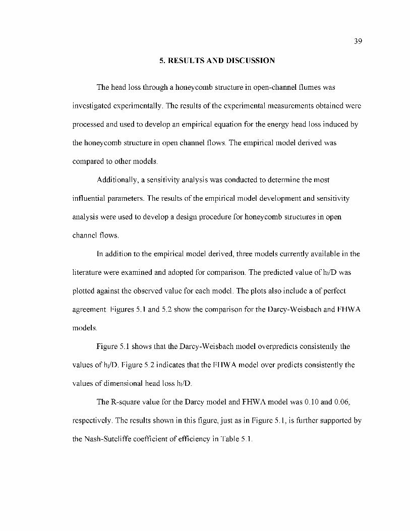
5. RESULTS AND DISCUSSION
The head loss through a honeycomb structure in open-channel flumes was
investigated experimentally. The results of the experimental measurements obtained were
processed and used to develop an empirical equation for the energy head loss induced by
the honeycomb structure in open channel flows. The empirical model derived was
compared to other models.
Additionally, a sensitivity analysis was conducted to determine the most
influential parameters. The results of the empirical model development and sensitivity
analysis were used to develop a design procedure for honeycomb structures in open
channel flows.
In addition to the empirical model derived, three models currently available in the
literature were examined and adopted for comparison. The predicted value of hi/D was
plotted against the observed value for each model. The plots also include a of perfect
agreement. Figures 5.1 and 5.2 show the comparison for the Darcy-Weisbach and FHWA
models.
Figure 5.1 shows that the Darcy-Weisbach model overpredicts consistently the
values of hi/D. Figure 5.2 indicates that the FHWA model over predicts consistently the
values of dimensional head loss hi/D.
The R-square value for the Darcy model and FHWA model was 0.10 and 0.06,
respectively. The results shown in this figure, just as in Figure 5.1, is further supported by
the Nash-Sutcliffe coefficient of efficiency in Table 5.1.

hl/D
(Ex
p)
hl/D
(Ex
p)
40
20
15
10
5
hl/D (Darcy)
Figure 5.1 The Predictability of the Darcy-Weisbach Model.
FHWA Predictability
Figure 5.2 The Predictability of the FHWA Model.

41
Table 5.1 Model Performance.
Model NSE
Empirical 0.75
Darcy -72939
FHWA -53526
Eckert -16.2
Figure 5.3 shows the plot for the Eckert Model. The plot shows that the model
somewhat predicts the values of hi/D. The plot suggests that the form of the equation is
useful, but some adjustments may need to be made. The R-square value for the Eckert
model was 0.20. The outlier results in the plot occurred in the test series D=1/2. This
suggests that the model will under predict the head loss through honeycombs with
diameters less than % inches.
Figure 5.4 shows the plot for the empirical model. The plot shows that the model
predicts the value of hi/D for the range of parameters tested. The R-square value for the
empirical model was 0.76. This figure further supports the usefulness of the empirical
model.

hi/D
(Exp)
hL
(Exp
)
42
Eckert Predictability
hL (Eckert)
Figure 5.3 The Predictability of the Eckert Model.
Empirical Model Predictability
hl/D (Empirical)
Figure 5.4 The Predictability of the Empirical Model.

43
The experimental observations of the parameter hi/D were plotted versus the
1/2 5/2parameter Diameter Froude Number, Q/(g D ). The plots were separately prepared for
different values of w/D and for different values of the ratio L/D. These plots show that
1/2 5/2the parameter hi/D increases with increases of Q/(g D ) and that greater values of the
L/D parameter translate into greater values hi/D. The plots in Figures 5.1-5.6 depict the
observed trend of the value of hi/D versus the other noted parameters.
The figures show that a greater L/D results in a greater value of hi/D.
Additionally, Figures 5.5-5.10 show that as the discharge increases for a given structure,
the head loss also increases. The figures also show that decreasing the diameter of the
pipes increases the head loss.
0.08
0.07
0.06
0.05
5. 0.04
0.03
0.02
0.01
0.00o.<
w/D = 1
- ■ - L / D = 2
—• — L/D = 1
X) 0.01 0.02 0.03 0.04 0.05 0.06 0.07 0.08
Q /(g 1/2D 5/2)
Figure 5.5 The Plot of hi/D vs Q/(g12D5 2) for w/D = 1.

44
0.18
0.16
0.14
0.12
~ 0.10
^ 0.08
0.06
0.04
0.02
0.00o.<
w/D = 1-1/3
- B - L / D = 2-2/3
- « - L / D = 1-1/3
A L/D = 2/3
10 0.02 0.04 0.06 0.08 0.10 0.12 0.14 0.16
Q /(g 1/2D 5/2)
Figure 5.6 The Plot of hi/D vs Q/(g12D5 2) for w/D = 1-1/3.
0.07
0.06
0.05
0.04
^ 0.03
0.02
0.01
0.00o.<
w/D = 1-1/2
------- ■
—■—L/D = 1
- • - L / D = 1/2
1610 0.02 0.04 0.06 0.08 0.10 0.12 0.14 0.
Q /(g 1/2D 5/2)
Figure 5.7 The Plot of hi/D vs Q/(g12D5 2) for w/D = 1-1/2.

45
w/D = 20.25
0.20
0.15
■*30.10
0.05
-L/D = 4
-L/D = 2
-L/D = 1
0.000.00 0.05 0.10 0.15 0.20
Q /(g 1/2D 5/2)
0.25 0.30
Figure 5.8 The Plot of hi/D vs Q/(g12D5 2) for w/D = 2.
0.09
0.08
0.07
0.06
~ 0.05
0.04
0.03
0.02
0.01
0.00o.<
w/D = 2.4
- ■ - L / D = 1.6
- • - L / D = 0.8
5010 0.10 0.20 0.30 0.40 0.:
Q /(g 1/2D 52)
Figure 5.9 The Plot of hi/D vs Q/(g12D5 2) for w/D = 2.4.

46
0.14
0.12
0.10
0.08
^ 0.06
0.04
0.02
n nn
w/D == 3
—■—L/D = 2
—• — L/D = 1
0.00 0.10 0.20 0.30 0.40 0.50
Q /(g 1/2D 5/2)
Figure 5.10 The Plot of hi/D vs Q/(g12D5 2) for w/D = 3.
The empirical model, Equation 31, and the figures above, Figure 5.5 to 5.10,
serve as design tools for honeycomb structures in open channel flows. For the range of
parameters tested, the empirical model can be solved directly for a given unknown if the
other parameters are provided. In situations with multiple unknown parameters, Figures
5.5-5.10 provide design charts. Given a discharge and channel geometry, the pipe
diameter is selected, and the parameter w/D is determined. The corresponding w/D chart
will then provide information to select the pipe length for the honeycomb structure. The
model equation and the charts will also allow the discharge to be determined if the
geometry of the channel and the honeycomb structure are known as well as the head loss
through the structure.

47
6. CONCLUSIONS AND RECOMMENDATIONS
The results of this work provide a means to predict the head loss through a
honeycomb structure in an open channel. Additionally, a procedure for designing
structures was also outlined. Multiple approaches were considered, and the empirical
model was found to be best suited to predict the energy head loss across the honeycomb
structure.
This work found that the application of currently available models was
insufficient to predict accurately head loss. Both the applied Darcy-Weisbach and the
FHWA models over-predicted the head loss for the structure. The Eckert model showed
some potential for application; however, some adjustments will be required for
improvement. All the considered existing models produce negative NSE values, which
indicate poor prediction ability. The empirical model developed from the statistical
analysis of the collected data best predicted the head loss. The model had NSE values of
0.83 and 0.75 for the development and validation data respectively.
The empirical model was most sensitive to the y/D parameter. The value of hi/D
increased and decreased by the same percentage as y/D. Increasing and decreasing the
value of L/D caused an increase and decrease of hi/D by half the percentage of change in
L/D. The value of hi/D decreased and increased one fifth the percentage of increase and
decrease in w/D. The FrD parameter was shown to change the value of hi/D one fifteenth
of the percentage of the change of FrD. The most influential parameter was shown to be
y/D while the least influential parameter was shown to be FrD.

The experimental work showed general trends in the head loss for given
parameters. For a given w/D, increasing L/D resulted in increased hi/D. For a given w/D
and L/D, increasing the discharge resulted in an increase in hi/D. The results also showed
that decreasing the diameter lead to an increase in the head loss. The results provide
general design guidance for honeycomb structures.
The result of this work provided an empirical model and charts for design. The
empirical model directly calculates the head loss when the discharge, width, flow depth,
pipe length and pipe diameter are known. Figures 5.5-5.10 are design charts and narrow
down possible dimensions for a given application. The work resulted in a design
procedure for honeycomb structures. First, the design discharge and channel geometry
are collected. The width of the channel is in feet and the design discharge is in cubic feet
per second. Then a pipe diameter is selected, in inches, and the corresponding design
chart is considered. The design chart is then used to select a length of pipe, in feet, to
meet the design requirements. Finally, the head loss, in feet, for a given discharge
through the selected structure geometry can be predicted using the model. It should be
noted that the empirical model was determined from the range of parameters examined.
The empirical model is valid for a range of discharges from 0.053 to 4.310 cubic feet per
second, a range of pipe diameters from ^ to 2 inches, a range of pipe lengths from 0.5 to
2 feet, a range of y/D from 1 to 5, and a range of channel widths from 1 to 3 feet. The
greatest impact on the predicted head loss is the parameter, y/D. y/D represents the flow
depth, in inches, to pipe diameter in inches.
This work evaluated honeycomb structures in a wide range of discharges and
geometries and provided design guidance for applications within these ranges. The
48

49
performance of honeycombs of different materials, orientations, and in larger discharges
has yet to be investigated. Additionally, the impact of honeycomb structures on the
erosion of a bed of erodible material, the impact of the combination of honeycombs and
screens, and the calibration of the Eckert’s model equation for honeycombs in open
channel flows have yet to be investigated.

50
BIBLIOGRAPHY
1. Prandtl, L., Attaining a steady air stream in wind tunnels. 1933.
2. Barlow, J.B., W.H. Rae, and A. Pope, Low-Speed Wind Tunnel Testing. Third ed. 1999: John Wiley & Sons.
3. Scheiman, J. and J. Brooks, Comparison o f experimental and theoretical turbulence reduction from screens, honeycomb, and honeycomb-screen combinations. Journal of Aircraft, 1981. 18(8): p. 638-643.
4. Idelcik, I., Handbook o f hydraulic resistance: coefficients o f local resistance and offriction. 1966, ERDA Div. Phys. Res.
5. Lumley, J., Passage o f a turbulent stream through honeycomb o f large length-to- diameter ratio. 1964.
6. Lumley, J.L. and J. McMahon, Reducing water tunnel turbulence by means o f a honeycomb. 1967.
7. Jiang, Y., et al. The hydrodynamic design and critical techniques for 1mx 1m water tunnel. in AIP Conference Proceedings. 2018. AIP Publishing LLC.
8. Yeh, H.H. and M. Shrestha, Free-surface flow through screen. Journal of Hydraulic Engineering, 1989. 115(10): p. 1371-1385.
9. £akir, P., Experimental investigation o f energy dissipation through screens. 2003, Citeseer.
10. Tsikata, J.M., Experimental investigation o f turbulent flow through trashracks. 2008.
11. White, F.M., Fluid Mechanics. Fourth ed. 2010: McGraw-Hill.
12. Transportation, T.D.o., Hydraulic Design Manual. 2019, TxDOT Austin, Tex.: Austin, Texas, United States of America.
13. Mays, L.W., Water resources engineering. Second ed. 2010: John Wiley & Sons.
14. Mohammed-Ali, W., Hydraulic characteristics o f semi-elliptical sharp crested weirs. J. Int. J. v. Giraldez Rev. Civil Eng, 2012. 1: p. 13.
15. Nash, J.E. and J.V. Sutcliffe, River flow forecasting through conceptual models part I—A discussion o f principles. Journal of hydrology, 1970. 10(3): p. 282-290.

51
16. Mohammed-Ali, W., C. Mendoza, and R.R. Holmes Jr, Influence of hydropower outflow characteristics on riverbank stability: case o f the Lower Osage River (Missouri, USA). Hydrological Sciences Journal, 2020.
17. Mohammed-Ali, W., C. Mendoza, and R.R. Holmes, Riverbank stability assessment during hydro-peak flow events: The lower Osage River case (Missouri, USA). International Journal of River Basin Management, 2020: p. 1-9.

52
VITA
Kyle David Hix received his B.S. in Civil Engineering in December 2018 from
Missouri University of Science and Technology. He also received his M.S. in Civil
Engineering from Missouri University of Science and Technology in August 2020.