experimental investigation of the agitation …etd.lib.metu.edu.tr/upload/12607412/index.pdf ·...
TRANSCRIPT

i
EXPERIMENTAL INVESTIGATION OF THE AGITATION OF COMPLEX FLUIDS
A THESIS SUBMITTED TO THE GRADUATE SCHOOL OF NATURAL AND APPLIED SCIENCES
OF MIDDLE EAST TECHNICAL UNIVERSITY
BY
ÖZGE YAZICIOĞLU
IN PARTIAL FULFILLMENT OF THE REQUIREMENTS FOR
THE DEGREE OF MASTER OF SCIENCE IN
CHEMICAL ENGINEERING
JULY 2006

ii
Approval of the Graduate School of Natural and Applied Sciences
Prof. Dr. Canan Özgen
Director
I certify that this thesis satisfies all the requirements as a thesis for the degree of Master of Science.
Prof. Dr. Nurcan Baç Head of Department
This is to certify that we have read this thesis and that in our opinion it is fully adequate, in scope and quality, as a thesis and for the degree of Master of Science.
Asst. Prof. Dr. Yusuf Uludağ
Supervisor
Examining Committee Members
Prof. Dr. Ufuk Bakır (METU, CHE)
Asst. Prof. Dr. Yusuf Uludağ (METU, CHE)
Prof. Dr. Pınar Çalık (METU, CHE)
Asst. Prof. Dr. Halil Kalıpçılar (METU, CHE)
Dr. Ömür Uğur (METU, IAM)

iii
PLAGIARISM
I hereby declare that all information in this document has been obtained and presented in accordance with academic rules and ethical conduct. I also declare that, as required by these rules and conduct, I have fully cited and referenced all material and results that are not original to this work.
Name, Last Name : Özge YAZICIOĞLU
Signature :
iv
ABSTRACT EXPERIMENTAL INVESTIGATION OF THE AGITATION OF COMPLEX
FLUIDS
YAZICIOĞLU, Özge
M.Sc. Department of Chemical Engineering
Supervisor: Asst. Dr. Yusuf Uludağ
July 2006, 159 pages
In this study, agitation of solutions using different impeller and tank geometry
were investigated experimentally in terms of hydrodynamics, macromixing time
and aeration characteristics. In the first set of experiments a cylindrical vessel
equipped with two types of hydrofoil and a hyperboloid impeller or their
combinations were used. Vessel and impeller diameters and water level were
300, 100 and 300 mm, respectively. At the same specific power consumption,
163 W/m3, the so called “hydrofoil 1” impeller provided the shortest mixing time
at 7.8 s. At the top hydrofoil 1 impeller submergence of 100 mm, the
hyperboloid impeller combination of it was the most efficient by a mixing time of
10.0 s at 163 W/m3. Ultrasound Doppler velocimetry and the lightsheet
experiments showed that the hydrofoil 1, hydrofoil 2 impellers and the stated
impeller combination provided a complete circulation all over the tank.
Macromixing measurements were performed in square vessel for Generation 5
low and high rib and Generation 6 hyperboloid impellers. Vessel length, impeller
diameters and water level were 900, 300 and 450 mm, respectively. At the same
v
specific power consumption, 88.4 W/m3, Generation 6 mixer provided the lowest
mixing time at 80.5 s.
Aeration experiments were performed in square tank for Generation 5 low rib
and Generation 6 hyperboloid impellers equipped with additional blades. With
increasing flow number, the differences between the performances at different
rotational speeds became smaller for each type of mixer. At similar conditions
the transferred oxygen amount of Generation 6 impeller was about 20% better.
Keywords: Macromixing time, ultrasound Doppler velocimetry, light sheet,
hydrofoil impeller, hyperboloid impeller, aeration, oxygen transfer

vi
ÖZ
KOMPLEKS SIVILARIN KARIŞTIRILMASININ DENEYSEL OLARAK
İNCELENMESİ
Yazıcıoğlu, Özge
Yüksek Lisans, Kimya Mühendisliği Bölümü
Tez Yöneticisi: Asst. Dr. Yusuf ULUDAĞ
Temmuz 2006, 159 sayfa
Bu çalışmada, solüsyonların karıştırılması değişik karıştırıcı ve tank geometrileri
kullanılarak hidrodinamik, makrokarıştırma zamanı ve havalandırma
karakteristiği açısından incelenmiştir. Deneylerin ilk bölümünde iki hidrofoil ve bir
hiperboloid karıştırıcı ve bunların kombinasyonları kullanılmıştır. Tank ve
karıştırıcı çapları ve su seviyesi sırasıyla 300, 100 ve 300 mm’dir. Aynı spesifik
güç harcamasında (163 W/m3) hidrofoil 1 karıştırıcısının 7.8 s ile en az karıştırma
zamanını sağladığı belirlenmiştir. Üst hidrofoil 1 karıştıcının su yüzeyinden 100
mm alçakta olduğu durumda, hiperboloid kombinasyonunun 163 W/m3’lik
spesifik güç tüketiminde 10.0 s’lik karıştırma zamanı ile en verimli konfigürasyon
olarak belirlenmiştir. Ultrasonik Doppler hızölçüm ve ışık kesiti deneyleri hidrofoil
1, hidrofoil 2 karıştırıcılar ve belirtilen karıştırıcı kombinasyonunun tüm tankta
tam bir sirkulasyon sağladığını göstermişlerdir.
Makro karıştırma ölçümleri kare tankta, 5.nesil alçak ve yüksek damarlı ve 6.
nesil hiperboloid karıştırıcılar için gerçekleştirildi. Tank ve karıştırıcı çapları ve su
seviyesi sırasıyla 900, 300 ve 450 mm’dir. Aynı spesifik güç harcamasında (88,4
vii
W/m3) 6. nesil hiperboloid karıştırıcısının 80,5 s ile en az karıştırma zamanını
sağladığı belirlenmiştir.
Havalandırma deneyleri kare tankta ilave bıçaklı 5. jenerasyon (alçak damarlı) ve
6. jenerasyon hiperboloid karıştırıcılar için gerçekleştirildi. Akış numarası
yükseldikçe her bir karıştırıcı için değişik dönme hızlarında performanslar
arasındaki fark azalmaktadır. Benzer şartlarda 6. jenerasyon karıştırıcının
aktarılan oksijen miktarı açısından 5. jenerasyon (alçak damarlı) karıştırıcıya
göre % 20 civarında daha yüksek olduğu belirlenmiştir.
Anahtar Kelimeler: Karıştırma zamanı, ultrasonik Doppler hız ölçümü, ışık kesiti,
hidrofoil karıştırıcı, hiperboloid karıştırıcı, havalandırma, oksijen transferi

viii
To my parents,
DEDICATION

ix
ACKNOWLEDGEMENTS
I wish to express my deepest gratitude to my thesis supervisors Assoc. Prof.
Yusuf Uludağ for all his understanding, patience, support and sound advice in all
aspects of my research work. I am very much obliged for his objective attitude,
creating very pleasant working conditions.
I should mention, Korhan Erol, Çiğdem Çuhadar, Walter Steidl, Ute Pirner, Ursula
Fink, my laboratory mate Ahmed Nassar, my dear parents Suzan and Yılmaz
Yazıcıoğlu and my dear sisters Eylem and Ezgi Yazıcıoğlu, and many others that I
could not mention here, who gave me helpful suggestions for the improvement
of the document and moral support.
I would like to thank Dr. Marcus Höfken for providing me the opportunity to work
at Invent Umwelt-und Verfahrenstechnik AG’s laboratories.
Thanks are due to all the staff of Invent Umwelt und Verfahrenstechnik AG and
Chemical Engineering Department.

x
TABLE OF CONTENTS
PLAGIARISM ............................................................................................. iii
ABSTRACT ................................................................................................iv
ÖZ...........................................................................................................vi
DEDICATION........................................................................................... viii
ACKNOWLEDGEMENTS ...............................................................................ix
TABLE OF CONTENTS ................................................................................. x
LIST OF TABLES ...................................................................................... xiv
LIST OF FIGURES .................................................................................... xvi
LIST OF SYMBOLS ....................................................................................xx
CHAPTER
1. INTRODUCTION ..................................................................................... 1
2. THEORETICAL BASICS OF MIXING AND AERATION..................................... 6
2.1. Turbulence and Flow Field in Agitated Tanks........................................ 6
2.1.1. General Properties of Turbulent Flow............................................ 6
2.1.2. Important Dimensionless Numbers in Mixing ................................10

xi
2.1.3. Power Consumption in Turbulent Mixing ......................................12
2.1.4. Macromixing and Mixing Time ....................................................14
2.1.5. Homogenization and Discharge Characteristics of the Impellers ......17
2.1.6. Mixing and Pumping Efficiency of the Impellers ............................18
2.2.1. Theoretical Considerations .........................................................20
2.2.2. Mass transfer in aeration ...........................................................21
2.2.2. Parameters for the oxygen transfer and aeration system ...............22
3. ULTRASOUND DOPPLER VELOCIMETRY AND LIGHSHEET FLOW
VISUALIZATION TECHNIQUES....................................................................24
4. LITERATURE REVIEW ON MIXING AND AERATION.....................................37
4.1. Power Consumption and Macromixing Time........................................37
4.1.1. Impeller Design ........................................................................37
4.1.2. Impeller Clearance....................................................................42
4.1.3. Mixing Time Measuring Technique...............................................43
4.2. Ultrasound Doppler Measurements....................................................45
4.3. Lightsheet Experiments ...................................................................50
4.4. Aeration ........................................................................................50
5. EXPERIMENTAL WORK...........................................................................54
5.1. Set-up of Cylindrical Tank Experiments..............................................54
5.1.1. Drive motor .............................................................................55
5.1.2. Mixing tank..............................................................................55
xii
5.1.3. Mixers .....................................................................................57
5.1.4. Conductivity meter & Amplifier ...................................................59
5.1.5. Torquemeter ............................................................................59
5.1.6. Ultrasound Doppler Velocimeter..................................................60
5.2. Experimental Procedures for Cylindrical Tank Experiments ...................61
5.2.1. Power Consumption Measurements .............................................61
5.2.2. Macromixing Time Measurements ...............................................62
5.2.2.1. Measurement Procedure ......................................................62
5.2.2.2. Macro Mixing Time Calculation Procedure...............................63
5.2.3. Ultrasound Doppler Velocimeter Measurements ............................66
5.2.3.1. Calculation Procedure for the UDV Measurements ...................68
5.2.4. Lightsheet Experiments .............................................................69
5.3. Square Tank Experiments ................................................................70
5.3.1. Mixers .....................................................................................71
5.3.2. Determination of the macromixing time.......................................73
5.3.3. Aeration Experiments ................................................................75
6. RESULTS AND DISCUSSION ...................................................................78
6.1. Cylindrical Tank Results ...................................................................78
6.1.1. Power Consumption ..................................................................78
6.1.2. Macromixing Measurements ..........................................................81
6.1.2.1. Comparison of the Mixing Time Results with Correlations.........88
6.1.3. Ultrasound Doppler Measurements..............................................92
6.1.3.1. Results of Hydrofoil 1 Impeller .............................................93
xiii
6.1.3.2. Results of Hydrofoil 2 Impeller .............................................98
6.1.3.4. Results of Combination 1 (submergence of the top hydrofoil
impeller = d)................................................................................103
6.1.3.5. Results of Combination 2 (submergence of the top hydrofoil
impeller = 1.5d) ...........................................................................108
6.1.4. Flow Visualization (Lightsheet) Experiments...............................113
6.2. Square Tank Experiments ..............................................................119
6.2.1. Macromixing Measurements in the Square Tank .........................119
6.2.2. Results of Aeration Experiments ...............................................122
7. CONCLUSIONS ...................................................................................130
8. RECOMMENDATIONS...........................................................................132
REFERENCES..........................................................................................134
APPENDICES
A. POWER CONSUMPTION DATA FOR CYLINDRICAL TANK MEASUREMENTS ...140
B. MACROMIXING TIME DATA FOR CYLINDRICAL TANK MEASUREMENTS.......145
C. MACROMIXING TIME DATA FOR SQUARE TANK MEASUREMENTS ..............148
D. AERATION DATA FOR SQUARE TANK MEASUREMENTS ............................150
E. ANALYSIS OF TORQUE AND ROTATIONAL SPEED DATA ...........................154
F. DISSOLVED OXYGEN MEASUREMENT PROCEDURE ..................................155
G. LIGHTSHEET MOVIES OF THE CYLINDRICAL TANK EXPERIMENTS...front cover

xiv
LIST OF TABLES
TABLES
1.1 Classification System for Mixing Processes ....................................... 2
3.1 Maximum Depth and Velocity data for US probes ............................30
3.2 Pmax, Fprf and ∆T values for water ...............................................34
4.1 Working fluids and tracer particles used in some UDV researches.......49
4.2 Particle types for the laser-lightsheet..............................................50
5.1 Dimensions of the cylindrical stirred tank configuration.....................55
5.2 Dimensions of the investigated impellers.........................................57
5.3 Specifications of hydrofoil 1 impeller...............................................58
5.4 Specifications of hydrofoil 2 impeller...............................................59
5.5 Depths and the maximum measurable velocities in UDV system ........60
5.6 Dimensions of the rectangular stirred tank ......................................71
5.7 Dimensions of the impellers used in the experiment .........................72
5.8 Newton numbers of the impellers ..................................................74
6.1 Dimensionless mixing time numbers of the investigated impellers .....87
6.2 Mixing times at the same power consumption for the investigated
impellers ..........................................................................................87
6.3 Mixing time and specific power data for the investigated impellers ...121
A.1 Experimental Power Consumption Data of Hydrofoil 1 Impeller .......140
A.2 Experimental Power Consumption Data of Hydrofoil 2 Impeller .......141
xv
A.3 Experimental Power Consumption Data of Hyperboloid Impeller ......142
A.4 Experimental Power Consumption Data of Hydrofoil 1 and Hyperboloid
Impeller Combination (d) .................................................................143
A.5 Experimental Power Consumption Data of Hydrofoil 1 and Hyperboloid
Impeller Combination (1.5d) ............................................................144
B.1 Experimental Macromixing Time Data of 6 Blade Rushton Turbine ...145
B.2 Experimental Macromixing Time Data of Hydrofoil 1 Impeller ..........145
B.3 Experimental Macromixing Time Data of Hydrofoil 2 Impeller .........146
B.4 Experimental Macromixing Time Data of Hyperboloid Impeller .........146
B.5 Experimental Macromixing Time Data of Hydrofoil 1 and Hyperboloid
Impeller Combinations (d) ................................................................146
C.1 Experimental Macromixing Time Data of Generation 5 Hyperboloid (Low
Rib) Mixer .......................................................................................148
C.2 Experimental Macromixing Time Data of Generation 5 Hyperboloid (High
Rib) Mixer .......................................................................................148
C.3 Experimental Macromixing Time Data of Generation 6 ....................149
D.1 Experimental Aeration Data of Generation 5 (Low Rib) Hyperboloid
Mixer..............................................................................................150
D.2 Experimental Aeration Data of Generation 6 Hyperboloid Mixer.......152
xvi
LIST OF FIGURES
FIGURES
2.1 Macromixing time set-up and macromixing curve.............................16
3.1 UDV measurement on a flow with free surface .................................25
3.2 System components for Particle Image Velocimetry..........................36
5.1 Experimental Set-up for Mixing Time Experiments............................54
5.2 Stirred Tank Configuration ............................................................56
5.3 Hydrofoil 1 Impeller......................................................................57
5.4 Hydrofoil 2 Impeller......................................................................57
5.5 Hyperboloid Impeller ....................................................................58
5.6 Typical experimental concentration versus time response..................65
5.7 Axial UDV measurements ..............................................................67
5.8 Radial UDV measurements ............................................................68
5.9 Evaluation process of the UDV data ................................................69
5.10 Generation 5 Hyperboloid (low rib)...............................................72
5.11 Generation 5 Hyperboloid (high rib)..............................................73
5.12 Generation 6 Hyperboloid (front and bottom view) .........................73
5.13 Mixing time setup for the rectangular tank ....................................74
5.14 Front view of the mixer aerator....................................................76
6.1 Power characteristics of the investigated impellers ...........................80
6.2 Mixing time characteristics for the 6 blade Rushton turbine ...............81

xvii
6.3 Variation of dimensionless mixing time with Reynolds number in
cylindrical vessel................................................................................85
6.4 Variation of mixing time with rotational speed in cylindrical vessel
.......................................................................................................86
6.5 Comparison of the experimental results with the Ruszkowski correlation
estimations ......................................................................................89
6.6 Estimation of the mixing efficiency of the hydrofoil 1 impeller ............90
6.7 Estimation of the mixing efficiency of the hydrofoil 2 impeller ............91
6.8 Axial dimensionless velocities of hydrofoil 1 impeller.........................94
6.9 Axial turbulence of hydrofoil 1 impeller ...........................................95
6.10 Radial dimensionless velocities of hydrofoil 1 impeller.....................96
6.11 Radial turbulence of hydrofoil 1 impeller .......................................97
6.12 Axial dimensionless velocities of hydrofoil 2 impeller.......................99
6.13 Axial turbulence of hydrofoil 2 impeller .......................................100
6.14 Radial dimensionless velocities of hydrofoil 2 impeller...................101
6.15 Radial turbulence of hydrofoil 2 impeller .....................................102
6.16 Axial dimensionless velocities of hydrofoil 1 and hyperboloid
combination (d) ...............................................................................104
6.17 Axial turbulence of hydrofoil 1 and hyperboloid combination (d).....105
6.18 Radial dimensionless velocities of hydrofoil 1 and hyperboloid
combination (d) ...............................................................................106
6.19 Radial turbulence of hydrofoil 1 and hyperboloid combination (d) ...107
6.20 Axial dimensionless velocities of hydrofoil 1 and hyperboloid
combination (1.5d)...........................................................................109
6.21 Axial turbulence of hydrofoil 1 and hyperboloid combination (1.5d) 110

xviii
6.22 Radial dimensionless velocities of hydrofoil 1 and hyperboloid
combination (1.5d)...........................................................................111
6.23 Radial turbulence of hydrofoil 1 and hyperboloid combination (1.5d)
.....................................................................................................112
6.24 Lightsheet photo of the hydrofoil 1 impeller.................................114
6.25 Lightsheet photo of the hydrofoil 2 impeller.................................115
6.26 Lightsheet photo of the hyperboloid impeller ...............................116
6.27 Lightsheet photo of the mixer combination (d).............................117
6.28 Lightsheet photo of the mixer combination (1.5d) ........................118
6.29 The dependency of the macromixing time on rotational speed in
square tank.....................................................................................120
6.30 Macromixing time characteristics in square tank ..........................120
6.31 Variation of kLa with change of gas flow rate for Generation 5 low rib
impeller ..........................................................................................123
6.32 Variation of kLa with change of gas flow rate for Generation 6 impeller
.....................................................................................................124
6.33 Variation of OA [%] with Fl [-] at different rotational speeds for
Generation 5 ...................................................................................125
6.34 Variation of OA [%] with Fl [-] at different rotational speeds for
Generation 6 ...................................................................................126
6.35 Amount of oxygen transferred to the system at Fl=0.01 for Generation
5 and Generation 6 ..........................................................................127
6.36 Amount of oxygen transferred to the system at Fl=0.025 for
Generation 5 and Generation 6 ..........................................................128

xix
6.37 Amount of oxygen transferred to the system at Fl=0.04 for Generation
5 and Generation 6 ..........................................................................128

xx
LIST OF SYMBOLS
a : Specific interface area, 1/m
a, b : Constants, [-]
A : Gas liquid interface area, m2
Ar : Archimed number, [-]
bblade : Length of impeller blade (Hydrofoil Impellers), m
bhub : Length of impeller hub (Hydrofoil 2 Impeller), m
B : Baffle length, m
c : Sound velocity, m/s
cL : Concentration in the liquid phase, kg/m3
cs : Saturation concentration, kg/m3
cs,20 : Saturation concentration at 20°C, kg/m3
C : Distance of the baffle to the tank wall, m
C : Time dependent tracer concentration, mol/l
C : Final tracer concentration, mol/l
Cspeed : Speed coefficient, m/(s *Hz)
d : Impeller diameter, m
D : Tank diameter, m
D : Diffusion coefficient, cm2/s
DM : Molecular diffusivity, m2/s
DT : Turbulent diffusivity, m2/s
e : Specific power consumption, W/kg
fD : Doppler shift, Hz
xxi
f0 : Transmitting frequency, Hz
Fprf : Pulse repetition frequency, [kHz]
Fl : Primary flow number, [-]
Flc : Secondary flow number, [-]
Fr : Froude number, [-]
g : Accelaration of gravity, m/s2
hw : Water height in the aeration tank, m
H : Henry’s constant, bar
Hi : Water height in the tank, m
J : Diffusion flux, mol/m2s
k : Turbulent kinetic energy, m2/s2
kL : Global mass transfer coefficient obtained from the liquid side, m/s
kLa : Overall mass transfer coefficient, 1/s
K i : Constant, [-]
lblade : Width of the impeller blade (Hydrofoil Impellers), m
lhub : Width of the hub (Hydrofoil 2 Impeller), m
lk : Width of the impeller blade (Hydrofoil Impellers), m
lt : Width of the impeller blade (Hydrofoil Impellers), m
l : Length of square tank, m
κl : Kolmogoroff length scale, m
Tl : Turbulent length scale, m
L : Characteristic length scale, m
M : Mixing grade, [-]
.
M : Mass flow rate, kg/h
n : Rotational speed, 1/s
xxii
Ne : Newton number, [-]
Neturb : Turbulent Newton number, [-]
OA : Oxygen utilization efficiency, %
OC : Oxygen supply, [kg/h]
p : Pressure, [bar, Pa]
p : Depth of the particle, m
pi : Partial pressure of component i, bar, Pa
P : Power, W
Pmax : Maximum measurable depth, m
R : Universal gas constant (=8.31451), J/mol K
Q : Volumetric flow rate discharged from impeller tip, m3/h
Qc : Volumetric flow rate of the bulk of in the mixing tank, m3/h
QA : Air flow rate, m3/h
S : Baffle thickness, m
t : Time, s
td : Time delay between transmitted and received signal, s
tI : Integral length scale, s
tM : Characteristic time for mixing due to molecular diffusion, s
tT : Characteristic time for mixing due to turbulent diffusion, s
T : Temperature, °C
T : Torque, Nm
Tmeas : The measurement time for a single averaged profile, ms
Tsamp : Time between stored profiles, ms
Tsi : The time delay, ms
Tu : Turbulence intensity, [-]

xxiii
ueff : Effective value of the fluctuation velocity (RMS-Value), m/s
ui : Fluctuation velocity, m/s
uτ : Wall shear stress velocity, m/s
Ui : Flow velocity, m/s
Utip : Impeller tip velocity, m/s
V : Tank volume, m3
V : Velocity (in ultrasound), m/s
Vmax : Maximum measurable velocity component, m/s
wblade : Blade thickness, m
W : Diameter of the shaft, m
We : Weber number
x : Distance of scattering particle from transducer, m
Z : Impeller clearance, m
Greek Letters
α : Boundary layer factor, m/s
β : Mass transfer coefficient, m/s
δ : Phase shift (in ultrasound), [-]
T∆ : Averaged profile measuring time, s
ε : Energy dissipation rate, m2/s3
Eη : Pumping rate
θ : Surface renewal time in aeration, s
θ : Ultrasound wave incidence angle, °
xxiv
θ : Mixing time, s
λ : Taylor microscale, [-]
λ : Ultrasonic wavelength, m
Λ : Macroscale in mixing, m
µ : Dynamic viscosity, Pa.s
cµ : Continuous gas phase viscosity, Pa.S
υ : Kinematic viscosity, m2/s
ρ : Liquid density, g/cm3
cρ : Continious gas phase viscosity,kg/m3
σ : Surface tension, Pa
τ : Kolmogoroff microscale, [-]
τ : Shear stress acting on bubble, Pa
τturb : Turbulent shear stress, Pa
1
CHAPTER I
INTRODUCTION
Agitation is one of the most important unit operations in chemical process and
allied industries. The overall energy requirement of these processes forms a
significant part of the total energy and contributes toward major expenses. Fluid
mechanics prevailing in the mixers is complex, and hence the design procedures
have been empirical. Empirical correlations normally lead to significant
overdesign and result in inflated fixed and operating costs as well as in extra
start-up times. Further, the empiricism does not give rational answers to the
debottlenecking problems. Therefore, reliable procedures are needed for the
design of mixing equipment. In view of this, several attempts have been made in
the past, particularly during the last 35 years, to understand the mixing
phenomena both experimentally and theoretically (Nere, Patwarhan, and Joshi,
2003).
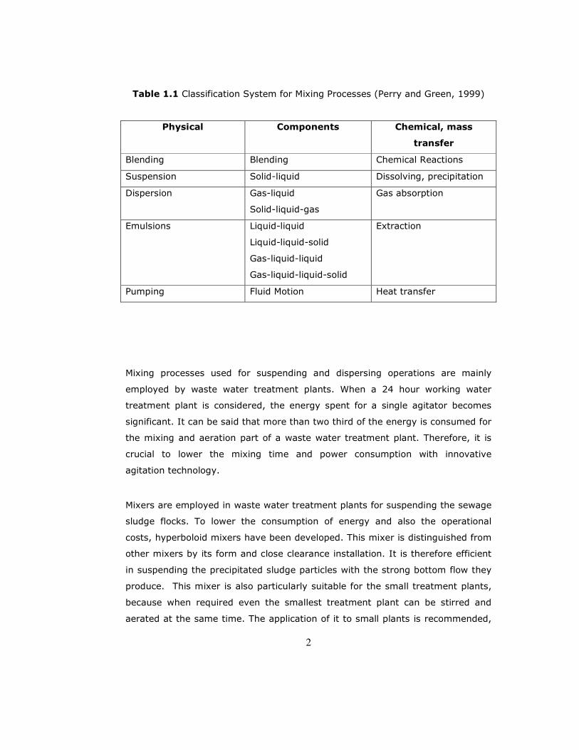
Major mixing applications of agitation are listed in Table 1.1. They are blending
(miscible liquids), liquid-solid, liquid-gas, liquid-liquid (immiscible liquids), and
fluid motion. There are also four other categories that occur, involving three or
four phases. One concept that differentiates between mixing requirements
originates from physical criteria listed in the second column of Table 1.1, in
various definitions of mixing requirements can be based on these physical
descriptions. The other category in Table 1.1 involves chemical and mass-
transfer criteria in which rates of mass transfer or chemical reaction are of
interest and have many more complexities in expressing the mixing
requirements (Perry and Green, 1999).
2
Table 1.1 Classification System for Mixing Processes (Perry and Green, 1999)
Physical Components Chemical, mass
transfer
Blending Blending Chemical Reactions
Suspension Solid-liquid Dissolving, precipitation
Dispersion Gas-liquid
Solid-liquid-gas
Gas absorption
Emulsions Liquid-liquid
Liquid-liquid-solid
Gas-liquid-liquid
Gas-liquid-liquid-solid
Extraction
Pumping Fluid Motion Heat transfer
Mixing processes used for suspending and dispersing operations are mainly
employed by waste water treatment plants. When a 24 hour working water
treatment plant is considered, the energy spent for a single agitator becomes
significant. It can be said that more than two third of the energy is consumed for
the mixing and aeration part of a waste water treatment plant. Therefore, it is
crucial to lower the mixing time and power consumption with innovative
agitation technology.
Mixers are employed in waste water treatment plants for suspending the sewage
sludge flocks. To lower the consumption of energy and also the operational
costs, hyperboloid mixers have been developed. This mixer is distinguished from
other mixers by its form and close clearance installation. It is therefore efficient
in suspending the precipitated sludge particles with the strong bottom flow they
produce. This mixer is also particularly suitable for the small treatment plants,
because when required even the smallest treatment plant can be stirred and
aerated at the same time. The application of it to small plants is recommended,

3
especially for isolated places or for coastal regions, because the building long
pipelines turns out to be unprofitable for such places (Steidl, 1995).
New design hydrofoil type impellers are also used in waste water treatment
plants because of the strong axial flow they produce. These types of impellers
are also used for suspending purposes. Especially, the hyperboloid and hydrofoil
combinations produce a strong top to bottom flow, and are usually used in water
treatment plants.
A good example of the gas absorption process (Table 1.1) which is accomplished
by the mixing process is the aeration systems in waste water treatment plants.
The dirtiness degree of the waste water discharged to the communal clarification
plants is characterized through BOD5 (Biological Oxygen Demand for 5 days)
value. This value forms the basis for the design and dimensioning of the required
oxygen entry for the biological degradation process of the organic part of the
waste water. Lowering the biological oxygen demand (BOD) and increasing the
dissolved oxygen (DO) level is achieved through the aeration systems in waste
water treatment plants.
The type of flow in an agitated vessel depends on the type of the impeller; the
characteristics of the fluid; and the size and proportions of the tank, baffles and
agitator. For a processing vessel to be effective, regardless of the nature of the
agitation problem, the volume of fluid circulated by the impeller must be
sufficient to sweep out the entire vessel in a reasonable time. Also, the velocity
of the stream leaving the impeller must be sufficient to carry the currents to the
remotest parts of the tank. In mixing and dispersion operations the circulation
rate is not the only factor, or even the most important one; turbulence in the
moving stream often governs the effectiveness of the operation. Turbulence
results from properly directed currents and large velocity gradients in the liquid.
Circulation and turbulence generation both consume energy. Although both flow
rate and power dissipation increase with stirrer speed, selection of the type and
size of the impeller influences the relative values of flow rate and power
dissipation (McCabe, Smith and Harriot, 1993).

4
A rotating impeller, which requires direct energy input, is the most important
part of the typical mixing equipment. The efficiency of the mixing process
depends on the design of the impeller (blade number, shape, and size). Also, the
location of the impeller (off-bottom clearance, distance from the vessel center,
i.e., eccentricity) and its size relative to the vessel have a profound impact on
the flow pattern and the mixing efficiency thereof (Nere, Patwarhan, and Joshi,
2003).
One of the objectives of this study is to investigate the efficiency of the hydrofoil
and hyperboloid impellers, as well as combinations of these, in the cylindrical
tank by power consumption and macromixing measurements. The conductivity
technique was used to determine the macromixing characteristics of the
impellers. This technique employs a probe which measures the conductance of
the salt solution as a function of time that can be converted to a concentration
versus time scale using calibration of the conductivity device.
Nere et al. (2003) emphasizes that extensive studies should be carried out in the
case of hydrofoil impellers. In this respect, this study will make a contribution to
the literature for the case of hydrofoil impellers. The investigations of the
combination of hydrofoil impellers with hyperboloid impellers will also be an
interesting contribution to the multiple impeller studies, e.g. to the work of Gao
et al. (2003) who investigated the macromixing characteristics of multiple
hydrofoil impellers.
The flow fields produced by the impellers in the cylindrical tank were determined
by the modern ultrasonic measuring technique, the so-called Ultrasonic Doppler
Velocimetry (UDV). Apart from determining the flow fields, locally produced
turbulence by the impellers could also be determined, so that conclusions for the
locally dissipated energy could be made. Lightsheet experiments, by which the
flow in the agitated tank can be visualized, were also performed for the
cylindrical tank. This combination of flow measuring technique and the
visualization of the flow itself permits a plastic illustration of the flow conditions
in the agitated tank and thus lead to a deeper understanding of the flow field
produced by the impellers. UDV and lightsheet techniques, which are non-

5
invasive and non-destructive, enabled direct visualization of complex flow field in
the agitated tanks. Therefore assessment of the agitation quality was possible
using the flow pattern in terms of circulation structure and dead volumes.
Another objective of this study is to investigate the efficiency of different types
of hyperboloid impellers, by macromixing measurements in a square tank,
whose geometry has been extensively employed in waste water treatment.
Two different hyperboloid mixers designed for aeration purposes were also
examined for their aeration characteristics in a stirred tank. The mixers were
provided with an aeration ring and the DO (Dissolved Oxygen) measurements
were performed in the stirred tank.

6
CHAPTER II
THEORETICAL BASICS OF MIXING AND AERATION
In this chapter theoretical basics of mixing and aeration in an agitated tank are
given. In the following parts, first the general properties of turbulent flow are
explained briefly, since typical agitation processes involve turbulent flow field.
Further the power consumption characteristics of an agitated tank as well as the
dimensionless numbers that are necessary and important in agitation are given.
Information about mixing will be followed with the part where the macromixing
and impeller characteristics are explained. Finally, theoretical basics of mass
transfer in aeration will be explained.
2.1. Turbulence and Flow Field in Agitated Tanks
2.1.1. General Properties of Turbulent Flow
Most of the flows that are common in industrial applications including agitation
are of turbulent type. Therefore it is beneficial to review general characteristics
of turbulence to understand the agitation process. In this section basics of the
turbulent flow in agitated tanks are described briefly based on various
researchers’ works.
Turbulence can result either from contact of a flowing stream with solid
boundaries or from contact between two layers of fluid moving at different

7
velocities (McCabe, Smith and Harriot, 1993). Turbulent flows have the following
properties:
• A flow is called turbulent when it passes the limit Recrit. If the Reynolds
number is smaller, the turbulence motions will be damped by frictional
forces.
• Turbulent flows dissipate energy as heat, that is, the energy must be
given from the outside for the fluctuating turbulent motions to prevail.
• The smallest element of a turbulent flow itself is large compared to the
length of the free path of the molecule. The equations of continuum
mechanics also apply for turbulent flows.
• Turbulent flows are three dimensional, friction containing eddy flows, in
which the inner friction play an important role for the formation of the
boundary layer contained in the eddies (Strauss, 1991).
• Altough the smallest eddies contain about 1012 molecules, all eddies are
of macroscopic size, and turbulent flow is not a molecular phenomenon.
• Turbulent flow consist of a mass of eddies of various sizes coexisting in
the flowing stream. Large eddies are continually formed. They break
down into smaller eddies, which in turn evolve still smaller ones. Finally,
the smallest eddies disappear (McCabe, Smith and Harriot, 1993).
• Mechanisms of turbulent flows are accidental, that is for the investigation
of such flows one should be leaded by statistical methods (Strauss,
1991).
Nagata (1975) explained the basic skeleton of the theory of turbulence primarily
from the book of Hinze (1959): The turbulence in a mixing vessel may not be
homogeneous, but the theory of local isotropy proposed by Kolmogoroff (1941)
may be applicable in general. Though the velocity and pressure at a certain point
in a turbulent field fluctuate irregularly, turbulence may be expressed as a
statistically continuous function with respect to time and space. Taylor (1935)
has shown that the Fourier transform of velocity correlation between two
adjacent points corresponds to an energy spectrum function which covers the
various scales of turbulence (Nagata, 1975).
8
The fluid in a turbulent flow can be considered as consisting of lumps and eddies.
The largest eddies have sizes of the same order of magnitude as the largest
length scale of the process equipment (vessel or impeller size, L ), whereas the
smallest eddies are such that viscous dissipation takes over and these smallest
eddies are dissipated into heat. Kolmogoroff length scale is characterized by
υκκκ /Re ul= ~ 1. The size of the smallest eddy is denoted by κl . The value of
κl depends on the turbulent energy dissipation rate per unit mass and the
kinematic viscosity of the fluid and is given by ( ) 4/13 / ευκ =l . There exists a
whole range of eddy sizes between L and κl , and this is usually represented by
an energy spectrum. Tennekes and Lumley (1972) have given an excellent
review of the structure of turbulence, the eddy sizes, their interrelations, the
energy spectra, etc. Brodkey (1966) has reviewed various aspects of turbulent
motion and its influence on mixing. Molecular diffusion takes place at the
Kolmogoroff scale and causes homogeneity at the scale of the smallest eddy,
while eddy diffusion is responsible for the transport of material at all of the
scales. The different size of eddies have different lifetimes. Depending on the
velocity, size, and lifetime, different eddies cause eddy dispersion to different
extents. All of these factors have to be taken into account while quantifying eddy
diffusion, and such a detailed analysis of the eddy dispersion process is
extremely complicated. To overcome these difficulties, eddy diffusion is usually
characterized in terms of eddy diffusivity. Eddy diffusion or molecular diffusion,
which is described in terms of diffusivity, is characterized by the corresponding
diffusion time. For molecular diffusion, the characteristic time is given as
MM Dlt /2
κ= . Similarly the characteristic time for eddy diffusion is TTT Dlt /2= . If
the diffusivities are known, then the mixing time Mθ or Tθ can be estimated
(Nere, Patwarhan, and Joshi, 2003).
In the turbulent flow range, macro scale eddies, which contain a larger part of
the turbulence energy, and micro scale eddies which contribute to the viscous
dissipation overlap with each other and give complicated effects upon various
phenomena in the mixing vessel. The larger eddies contain much less energy
than the smaller ones and reach only 20% of total kinetic energy at most. Eddies
9
which make contribution to the total kinetic energy of turbulence, are called the
energy containing eddies. The smallest eddies fluctuate and dissipate much more
rapidly than the large energy containing eddies (Nagata, 1975).
In a typical turbulent flow, large eddies continuously break into the smaller ones
and eventually become small enough to be dissipated by viscous effects. Energy
must then be continuously provided to the flow to maintain the turbulence. In
agitation energy is delivered to the tank content by means of impellers.
Brodkey (1966) states that any motion which might have a regular periodicity is
not considered to be turbulent. The instantaneous velocity at a point can be
represented by its average value and superimposed fluctuation:
U t U u ti i i( ) ( )= + ′ (2.1)
Instead of the velocity fluctuation usually the effective value, root-mean-square
(r.m.s.) value, of it is used:
( )u ueff = ′2 (2.2)
The relation between the effective value of the velocity fluctuation effu and the
time averaged velocity U i can be called turbulence intensity Tu :
Tuu
U
i
i
=′2
(2.3)
Turbulence intensity refers to the speed of the rotation of eddies and the energy
contained in an eddy of a specific size (McCabe, Smith and Harriot, 1993).
10
2.1.2. Important Dimensionless Numbers in Mixing
Throughout the application of dimensional analyses to the problems in the
agitation technology, it is observed that the dimensionless numbers enable the
information obtained in the laboratory scale to be transferred to the industrial
large scales. When the geometrical similarity is provided and the all the
dimensionless numbers are constant, the behavior of the operation at different
sizes is also similar. A further advantage of working with dimensionless numbers
is the independency of represented relations from the measure (Steidl, 1995). In
the following the most important dimensionless numbers concerning typical
agitation and mixing processes are given:”
Reynolds Number
The Reynolds number is determined from the ratio of inertial forces to viscous
force of the fluid. In fluid mechanics Reynolds number plays an important role in
the characterization of the flows. In the agitation technology, Reynolds number
is formed mainly with the mixer diameter d , tip speed tipU and kinematic
viscosity υ :
υ
π
υ
2dndU
Retip ⋅⋅
=⋅
= (2.4)
If the Reynolds number is > 104, a fully turbulent agitator flow occurs. With the
Reynolds number < 100, flow becomes laminar. Within the region 100 < Re <
104, the flow field in the tank exhibits transition characteristics.
11
Froude Number
Another important dimensionless number for characterization of the flow in a
stirred tank is the Froude number. It is the ratio of the inertial forces to gravity.
g
dnFr
⋅=
2
(2.5)
Archimed number
It is given by the following:
ArRe
Fr=
2
(2.6)
Newton Number
The Newton number Ne is the ratio of the agitator power P and the actual
power spent in the fluid:
53
dn
PNe
⋅⋅=
ρ (2.7)
It is depended on the stirred tank configuration and the Reynolds number. In the
turbulent region it remains nearly constant for a given tank configuration.
12
2.1.3. Power Consumption in Turbulent Mixing
Power draw is the energy per time which is transferred from the impeller to the
fluid. It is an integral quantity fundamental to mixing and dispersion processes
since energy is needed to cause the fluid motion necessary for mixing. For single
phase turbulent flow, power calculation has been mainly approached through
dimensional analysis and experimental measurement of torque.
Power basically has the same fundamental units as the product of ,, 3nρ and 5
d .
The dimensionless group for turbulent flow is typically 53/ dnP ρ and is called the
power number. For an agitated tank, a traditional relationship for power in the
form of a series of assumed power laws can be written as:
.....)()()()(22
53
dcbac
d
Z
d
D
g
dnndK
dn
Pg
µ
ρ
ρ= (2.8)
where a, b, c, d and K are constants.
The first dimensionless group is the impeller Reynolds number, the second is the
Froude number, and the rest accounts for the effects of geometry (i.e., impeller
clearance and baffle width) which includes number of effects (i.e., number of
blades, baffles and impellers) (Tatterson, 1991).
Turbulent flow is required, in order to obtain a high mixing grade of solutions,
except the high viscosity ones like pastes, in stirred tanks. In order to achieve a
high mixing grade standard baffled vessels are widely used.
Ciofalo et al. (1996) have explained the necessity for baffles as follows: If the
baffles which characterize the standard geometry are not supplied, the liquid
tends to move mainly along circular trajectories, resulting in small relative
velocities between impeller and fluid and weak radial flows directed towards the
13
tank walls. Installation of the baffles effectively destroys the circular liquid
patterns, inhibiting the vortex formation so that the liquid surface becomes
almost flat. Moreover, axial flows become much stronger, leading to an improved
mixing rate.
Working with turbulent flow in baffled tanks requires a high power input. In this
respect, determination of the two important values; power consumption and
mixing time is important. Experimental and predictive studies most of which are
focused on baffled tanks have been carried out in order to determine the stirred
tank characteristics.
In most of the experimental studies flow field in a stirred tank is measured in
details by the laser Doppler velocimetry (LDV) technique. Some of the
researchers who employed this technique for the investigation of stirred tanks
are Costes and Couderc (1988), Wu and Patterson (1989), Ranade and Joshi
(1990), Schäfer et al. (1997). Ultrasound Doppler velocimetry (UDV) has also
been employed by various researchers for the investigation of stirred tank
hydrodynamics, for example, Bouillard et al. (2001), Brito et al. (2001) and
Steidl (1995).
Computational Fluid Dynamics (CFD) technique is a cost effective design tool
which is also employed to study the turbulent flow in stirred vessels. However
turbulence and agitation are so complex in nature that this technique needs to
be much more developed possibly with high performance computing techniques,
but still, it remains as a challenging task.
Armenante et al. (1997) have stated that validation of CFD as a predictive tool
requires comparison of the numerical results with experimental velocity data. He
has added that most of the CFD work carried out to date, as far as flow in mixing
vessels is concerned, has been centered on applications dealing with baffled
vessels. Some of the predictions which have been presented are the studies of
Schäfer et al. (2004), Armenante et al. (1997), Ciofalo et al. (1996) and Kresta
and Wood (1993).
14
2.1.4. Macromixing and Mixing Time
The process of mixing occurs as a result of the motion at three levels: molecular
eddy and bulk motion. The molecular motion of individual species reduces the
concentration differences, and the process is known as molecular diffusion.
Mixing on this level is called micromixing. Improper micromixing leads to
segregation (Levenspiel, 1991). If the stirred reactor is operated under turbulent
conditions, then there is a motion of a chunk of molecules or eddies. The eddy
motion also gives rise to material transport and is called eddy diffusion or
dispersion. The bulk motion or the convective motion also has a property of
providing spread of materials needed for mixing. Usually, the bulk motion is
superimposed on either molecular or eddy diffusion or both. Mixing on this scale
is called macromixing (Nere et al., 2003). In this study, it is mainly dealt with
the large scale liquid-phase turbulent mixing, that is, macromixing.
The macromixing or blending time is the time required to mix the freshly
entering material with the contents of the whole vessel (www.scien
tificupdate.co.uk/pdfs/generic_pdfs/mixing.pdf, 2006). It corresponds to a
macroscopically determined mixing time if the macromixing time is much longer
than the micromixing time. In the turbulent regime this condition is satisfied
(Schäfer, 1999).
As stated above macromixing time (θ ) is the time required for the response at a
defined point to reach the required percent (mixing grade) of the total change
following a pulse injection. The mixing grade ( M ) is defined by the following
equations:
C
CM
∆−= 1 (2.9)
CCC −=∆ 2 (2.10)
15
where C is the time dependent tracer concentration and C is the final tracer
concentration. The macro mixing, referring to the value M=95 %, is terminated
as soon as ≤∆C 0.1 is observed.
For the determination of the macromixing time, there are different methods that
have already been applied. With physical measuring processes mixing grade up
to 95% can be reached in rule. On the other hand chemical measuring methods
provides the measurement of a whole mixing grade in the mixing tank. The
measured mixing time is dependent on the conditions of the experiment.
Especially, the dimension of the measuring probe, according to which the
dimensions of the volume element is determined, has an effect on the
determination of the concentration fluctuations. A detailed discussion on the
mixing grade and mixing time determination can be found in Hiby (1979) and
Nere et al. (2003). Different measuring processes have been analysed in Mann
et al. (1997) and Nere et al. (2003). In this study macromixing times were
determined by conductivity measurements, in which a conductivity probe is
employed to measure the conductivity change in the stirred tank. A typical
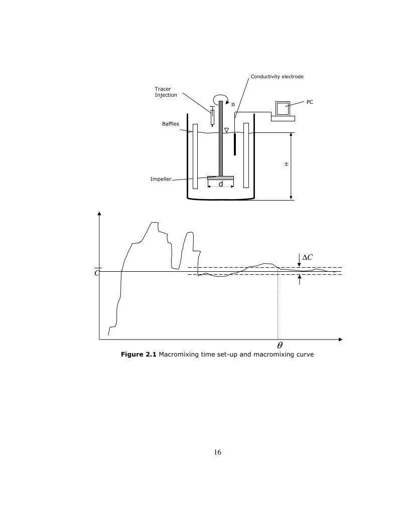
conductivity change set up is depicted in Figure 2.1 along with typical
concentration versus time response. Here the mixing time, θ denotes the point
at which ∆C≤0.1 condition is met.
16
Figure 2.1 Macromixing time set-up and macromixing curve
n
H
PC
d
Baffles
Impeller
Conductivity electrode
Tracer Injection
C∆
C
θ

17
2.1.5. Homogenization and Discharge Characteristics of the Impellers
When the Reynolds number is not small, discharge flow from the impeller
generates vertical circulation flow and gives a mixing action. The impellers can
be compared according to their discharge efficiency. The volumetric flow rate is
proportional to 3nd in the completely turbulent range (Nagata, 1975).
The mixing time which can be achieved by one mixer depends on the properties
of the fluid, diameter of the impeller and the rotational speed for a given
geometry. A dimesionanalytic investigation of this dependency provides the
homogenization characteristic, which is the process relationship between the
dimensionless mixing time –or homogenization- number θn and the mixing
Reynolds number Re .
Zlokarnik (1967) investigated the typical homogenization characteristic for
different inversely reversely proportional to the Reynolds number (i.e., θn ∝
Re/1 ) in laminar flow region for all types of impellers except the helical impeller.
In turbulent region, the dimensionless mixing time numbers have constant
values for the Reynolds numbers larger than 103-104. The value of this constant
depends on the form of the impeller and on the diameter relationship Dd / .
The homogenization characteristic is closely related to the pumping and
circulation efficiency of the mixers. The pumping power of the mixer is
determined from the standardized pumping rate which is called the primary flow
number. It is obtained from the mixer generated volumetric flow rate, Q , which
is the total flow leaving the impeller, measured at the tip of the blades:
3
nd
QFl = . (2.11)
18
Fl gives the discharge flow from the tips of the impeller and not the total flow
produced. The high-velocity stream of liquid leaving the tip of the impeller
entrains some of the slowly moving bulk liquid, which slows down the jet but
increases the total flow rate. The amount of the bulk fluid is greater than the
amount discharged from the impeller tips ( CQ >Q ). The entrainment is
considered in the secondary flow number, which is obtained from the circulation
flow:
3
nd
QFl C
C = . (2.12)
A general overview of the pumping rates can be found in Tatterson (1991) and
Fentiman et al’s (1998) works.
The circulation characteristics are often used to forecast the mixing time. The
detailed information for the formulation of circulation models can be found in
Khang et al. (1976) and Nienow (1997).
2.1.6. Mixing and Pumping Efficiency of the Impellers
Evaluation of the mixing and pumping efficiency of the impellers requires
information about the power input as well as the dimensionless pumping,
discharge and mixing time number data. Power characteristics of the impellers
describe a process relation between the power input and Reynolds number. The
Newton number remains constant in turbulent conditions, where the effect of
resistance can be neglected. A summary of the Newton number of different types
of impellers can be found in Tatterson’s (1991) work.
19
A relation between the pumping rates with the Newton number yields the
pumping efficiency of the impellers. The better the pumping efficiency, the less
power is required for pumping the same volumetric flow. The pumping efficiency
for impellers can be defined as follows:
43
11
=
D
d
Ne
FlEη (2.13)
A second dimensionless number for the secondary pumping rate is:
43
22
=
D
d
Ne
FlEη (2.14)
It is more reasonable to compare the impellers on the basis of 2Eη , because
total convective fluid transport and the energy input are considered in this case
(Schäfer, 1990).
2.2. Aeration
The agitation of gas-liquid systems has much application in physical and
chemical gas absorptions, for example, aerobic fermentation, waste water
treatment, catalytic hydrogenation of vegetable oils and oxidation of
hydrocarbons. In gas-liquid agitation, the following items must be considered:
• The state of dispersion, i.e., the size distribution of bubbles
• Gas hold-up and retention time in vessel
• Dispersion and coalescence of gas bubbles

20
• Convection currents and degree of backmixing
• Mass transfer across the interface of gas and liquid (Nagata, 1975).
2.2.1. Theoretical Considerations
Let us denote the diameter of gas bubbles by pd , shear stress acting on the
bubbles by τ , and the viscosity, density and interfacial tension by µ , ρ and
σ , respectively. Suffixes show the dispersed phase and the continuous phase
respectively. Forces acting on gas bubbles are: Shear stress, τ and surface
tension, pd/σ . When these two forces are equal, bubbles are in equilibrium
size. Therefore the maximum diameter of bubbles is determined by the ratio of
these forces, the Weber number:
σ
τ pdWe = . (2.15)
For bubbles ascending an descending in liquids, the ratio of lifting or settling
force ((1/6) gd p ρ∆ ) and surface tension is involved, and the We-number has the
form:
σ
ρ
6
2gd
Wep ∆
= . (2.16)
Concerning the dispersion of gases in mixing vessels, the shear stress due to
turbulence must be considered. The primary eddies produced by impellers have
scale (L) of similar magnitude to the dimension of the main flow. The large
primary eddies until finally their energy is dissipated into heat by viscous flow.
According to Kolmogoroff’s theory on the local isotropy, the scale ( κl ) of the
smallest eddies where the energy dissipation may occur is expressed by:
21
4/1
2/1
4/3
)/(−= VPl
c
c
ρ
µκ . (2.17)
2.2.2. Mass transfer in aeration
For the evaluation of the efficiency of aeration system in terms of mass transfer
the aeration coefficient kLa is used.
This system dependent constant can be determined with the help of theoretical
derivations and empirical experiments where the considerable parameters are
reduced. According to the theory of Higbie (1935) the following relation is given
for the aeration coefficient:
θπ ⋅
⋅=D
V
AakL 2 (2.18)
With this formula the parameters for the mass transfer in aeration can be
described as follows:
• A : Surface area
With pressurized air the surface A is the sum of the surface area of bubbles
present in the tank and of the water surface. The interface area is dependent on
the air flow rate and the retention time of the bubbles in the water. It is
inversely proportional to the bubble diameter.
• 1/θ : Surface renewal time
The velocity of the surface renewal is determined by mobility of the bubble
surface area.
• D : Diffusion coefficient of the oxygen in water (temperature dependent)
22
• V : Volume of the aerated water (constant).
Equation 2.18 is not for practical use for the calculation of the aeration
coefficient, since the value of surface area A and the value of the surface
renewal time θ are not possible observed. It can be said that the diffusion
coefficient as well as the parameters A and θ can be taken as constants at the
same waste water temperature.
2.2.2. Parameters for the oxygen transfer and aeration system
In waste water technology a couple of parameters are used for the design and
the evaluation of the aeration facilities. Some of these parameters are shortly
explained here.
According to the guidelines of ATV (1996), the oxygen supply is given as α -OC-
Value which is obtained from the amount of oxygen which is dumped into the
waste water per hour:
h
kgOOC 2=α (in waste water) (2.19)
Since the mass transfer efficiency of aeration systems are mostly examined with
clean water because of easier and safer methods, an additional OC value is
obtained for clean water conditions:
h
kgOOC 2= (clean water) (2.20)
The OCα -Value is obtained with the help of the α -Value:
23
),( stemaerationsywastewaterfOC
OC==
αα (2.19)
The α -Value depends on the properties of the waste water and on the aeration
system.
The OC-value is also shown as OC20-Value, since it is always obtained from clean
water at 20°C. Additionally, the OC20-Value is often obtained from the volume of
the sludge activation tank and given in the [kg O2/m3h] units. In this respect,
OC20-value does not give the required oxygen transfer, instead, it characterizes
the possible oxygen transfer of an aeration system (at 20°C in clean water),
which should be experimentally determined (Frey, 2000).
24
CHAPTER III
ULTRASOUND DOPPLER VELOCIMETRY AND LIGHSHEET
FLOW VISUALIZATION TECHNIQUES
3.1. UDV TECHNIQUE
There are different non-intrusive flow measurement techniques; these are briefly
laser Doppler velocimetry (LDV), ultrasonic Doppler velocimetry (UDV) and
nuclear magnetic resonance (NMR). LDV technique has a very high resolution
capability and the velocity component of a single particle which is perpendicular
to the axis of the light beam is measured. The maximum measurable velocity is
not limited and it does not require calibration. It cannot be used in non
transparent liquids and it is quite fragile. NMR technique has a high accuracy and
allows 2D and 3D measurements however its applications are quite expansive.
UDV technique has a lower resolution capability compared to LDV and the
velocity component which is in the direction of the axis of the ultrasonic beam is
measured. In this technique velocities of a great number of scatterers are
measured simultaneously and therefore the mean value of all the particles
present in the sampling volume are obtained. The maximum measurable velocity
and depth are limited in UDV. It does not also require calibration and contrary to
LDV it can be used in non transparent liquids and it is portable.
In UDV, instead of emitting continuous ultrasonic waves as in LDV, an emitter
sends periodically a short ultrasonic burst and a receiver collects continuously
echoes issues from targets that may be present in the path of the ultrasonic
beam. By sampling the incoming echoes at the same time relative to the
emission of the bursts, the shift of positions of scatterers are measured (Signal-

25
Processing SA, 2006). Schematic picture of UDV measurement is given in Figure
3.1.
Figure 3.1 UDV measurement on a flow with free surface (Met-Flow SA, 2005).
26
An ultrasonic transducer transmits a short emission of ultrasound (US), which
travels along the measurement axis mL , and then switches to the receiving
mode. When the US pulse hits a small particle in the liquid, part of the US
energy scatters on the particle and echoes back. The echo reaches the
transducer after a time delay
c
xtd
2= (3.1)
where dt is time delay between transmitted and received signal [s], x is the
distance of scattering particle from transducer [m] and c is the speed of sound
in the liquid [m/s].
If the scattering particle is moving with non-zero velocity component into the
acoustic axis Lm of the transducer, Doppler shift of echoed frequency takes place,
and received signal frequency becomes 'Doppler-shifted':
02 f
f
c
v d= (3.2)
where v is the velocity component into transducer axis [m/s], df is the Doppler
shift [Hz] and 0f is the transmitting frequency [Hz].
If UDV succeeds to measure the delay dt and Doppler shift df , it is then possible
to calculate both position and velocity of a particle. Since it is presumed that
scattering particles are small enough to follow the liquid flow, it can also be
presumed that the UDV has established the fluid flow component in the given
space point. The basic feature of UDV is the ability to establish the velocity in
many separate space points along measurement axis.
27
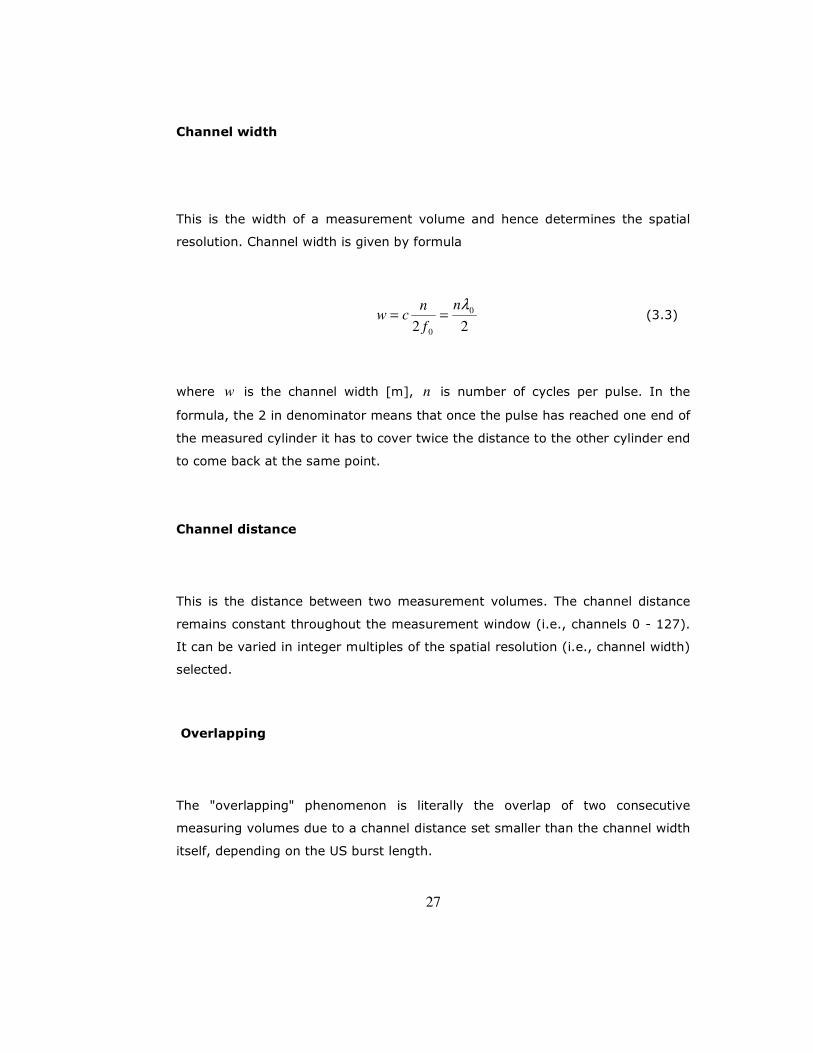
Channel width
This is the width of a measurement volume and hence determines the spatial
resolution. Channel width is given by formula
22
0
0
λn
f
ncw == (3.3)
where w is the channel width [m], n is number of cycles per pulse. In the
formula, the 2 in denominator means that once the pulse has reached one end of
the measured cylinder it has to cover twice the distance to the other cylinder end
to come back at the same point.
Channel distance
This is the distance between two measurement volumes. The channel distance
remains constant throughout the measurement window (i.e., channels 0 - 127).
It can be varied in integer multiples of the spatial resolution (i.e., channel width)
selected.
Overlapping
The "overlapping" phenomenon is literally the overlap of two consecutive
measuring volumes due to a channel distance set smaller than the channel width
itself, depending on the US burst length.

28
Measurement window
The measurement window is defined as the distance between channels 0
(starting channel) and 127 (window-end channel). This is given as
W = Starting channel + 127 * channel distance (3.4)
where W is the measurement window length [m]. The window-end position has
to be smaller than the maximum depth (that is, maximum depth >= W), so that
values are limited automatically when setting the channel distance and starting
position.
Maximum depth and Maximum velocity
The maximum measurable depth is determined by the pulse repetition frequency
prfF :
prfF
cP
2max = (3.5)
where maxP is the maximum measurable depth [m] and prfF is the pulse
repetition frequency [Hz].
The maximum depth decreases with increasing prfF . Due to the Nyquist
sampling theorem related to prfF , the maximum detectable Doppler shift

29
frequency is limited. This implies that there is a limitation on the maximum
velocity that can be measured. This limit is:
0
max4 f
cFV
prf= (3.6)
where maxV is the maximum measurable velocity component [m/s]. From the
above two equations, the following constraint can be obtained for this method of
measurement:
.8
*0
2
maxmax constf
cVP == (3.7)
Since for a given measuring situation both c and 0f are constant, the product
maxmax *VP is also constant. This means that, for a given transmitting frequency,
we have to compromise between maximum measurable depth, and maximum
measurable velocity.
Velocity resolution
We can now determine the velocity resolution. From the equation following
equations can be derived:
max0
2
max8 Pf
cV = (3.8)
30
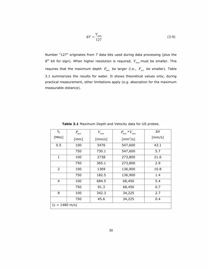
127
maxVV =∆ (3.9)
Number "127" originates from 7 data bits used during data processing (plus the
8th bit for sign). When higher resolution is required, maxV must be smaller. This
requires that the maximum depth maxP be larger (i.e., prfF be smaller). Table
3.1 summarizes the results for water. It shows theoretical values only; during
practical measurement, other limitations apply (e.g. absorption for the maximum
measurable distance).
Table 3.1 Maximum Depth and Velocity data for US probes.
f0
[MHz] maxP
[mm]
maxV
[mm/s]
maxP *maxV
[mm2/s]
∆V
[mm/s]
0.5 100 5476 547,600 43.1
750 730.1 547,600 5.7
1 100 2738 273,800 21.6
750 365.1 273,800 2.9
2 100 1369 136,900 10.8
750 182.5 136,900 1.4
4 100 684.5 68,450 5.4
750 91.3 68,450 0.7
8 100 342.3 34,225 2.7
750 45.6 34,225 0.4
(c = 1480 m/s)

31
Doppler Coefficient and the Speed Coefficient
The raw data, which is generated and recorded on the disk, is in units of
frequency detected during the measurement time. Thus the Doppler shift
frequency Df can be obtained from the raw data using the formula
Dopplerd Crawdataf *= (3.10)
where the Doppler coefficient, DopplerC , is given by
128*2
prf
Doppler
FC = (3.11)
The raw data is the data measured by UDV in internal units. Velocity along beam
axis is given by
dspeed fCv ⋅= (3.12)
and the speed coefficient is given by
02 f
cC speed = . (3.13)
where Cspeed is in the unit [m/(s *Hz) = m]. The data can be converted to a
velocity using the formula

32
θsin
1*** speedDoppler CCrawdataV = (3.14)
where θ is the US wave incidence angle normal to the flow [deg].
Flow direction
Since flow direction is detected at all measured positions, the measured data can
have both positive and negative values. A positive value means the flow
direction is in the beam direction (i.e., moving away from the transducer) and a
negative value means the opposite (i.e., moving toward the transducer). It is
possible to ignore this function; this being of value when the flow has only a
single direction (i.e., no recirculating eddies) and sign detection is not needed. In
this case, the 'aliasing' that arises when computing the Doppler shift frequency is
corrected, and the maximum detectable velocity is thereby doubled. 'Aliasing' in
this case means that two velocities (with the same values but different signs)
can exist for a single measured value of 'raw data'. It should be noted that when
sign detection is ignored, the constraint condition and the velocity resolution
described earlier become:
0
2
maxmax4 f
cVP =⋅ (3.15)
255
maxVV =∆ . (3.16)
33
This might be very useful in many circumstances. (Again, number "255"
originates from 8 data bits used during data processing with no bit necessary for
sign).
RF Gain
Since the attenuation of ultrasound in liquid and solid media follows an
exponential law, distant particles give weaker echo than particles closer to the
transducer. The amplification of the received echo is therefore adjusted so that
this attenuation is compensated for. The amplification is time dependent, and is
called the gain distribution. The RF gain factor modifies the slope of the gain
distribution. The gain distribution can be adjusted by setting its start and end
values. Both can be set from factor 1 to factor 9. When both are set at the same
value, the distribution is constant (flat). A factor of one is equivalent to 6dB.
US Emission Voltage
Overall amplification gain may also be controlled by changing the strength of
ultrasound emission through the change of voltage applied to the transducer
(namely US emission voltage). Depending on the kind of liquid, maximum depth,
condition of reflectors, etc., these parameters need to be optimized.
Time resolution
The time resolution of the measurement of a single profile is determined by the
data acquisition time, which itself depends on the pulse repetition frequency prfF
or the maximum depth. It is given by the number of repetitions repN used in the
Doppler shift calculation and:

34
prf
rep
F
NT =∆ (3.17)
where ∆ T is the averaged profile measuring time [s], repN is the number of
profile measurement repetitions (default = 32) and prfF is the pulse repetition
frequency [kHz]. Examples are given in the following table which are calculated
for c = 1480 m/s (water) and repN = 32 (default).
Table 3.2 Pmax, Fprf and ∆T values for water
Pmax
[mm]
Fprf
[kHz]
∆∆∆∆T
[ms]
100 7.4 4.3
200 3.7 8.6
750 0.987 32.4
Measuring time
In principle the time interval between measured profiles is equal to the time
resolution ∆T:
TTmeas ∆= . (3.18)

35
Sampling time
Sometimes it is useful for the user to slow down data acquisition. This can be the
case when longer time series are measured and the user wants to limit the data
file volume. This is why it is possible to set certain additional delay between
measured profiles. Sampling time is then
simeassamp TTT += (3.19)
where sampT is the time between stored profiles [ms], measT is the measurement
time for a single averaged profile [ms] and siT is the delay set by user [ms]
(Met-Flow SA, 2005).
3.2. LIGHTSHEET FLOW VISUALISATION TECHNIQUE
Applications of light sheet technique are widely used to obtain both quantitative
and qualitative information about a flow field in fluid dynamics. This technique
provides the visualization of flow along a projected line. In most light sheet
applications, different types of lasers, most of which are quite expensive, are
used as the light source. The experimental light sheet system is composed of a
linear light source, and a camera recorder. The scatterer particles are required to
be injected to the flow in order to enable the reflection. The particles become
visible along the light sheet so that the image formed can be recorded by a
camera. As the particle diameter of scatterers get smaller, they enable the
visualization of the smaller flow structures. The sensitivity of this technique
depends on the power of the light source, the sensitivity of the camera and the
scattering ability of the particles. Wang et al. (1997) have stated that this
technique suffered due to non-uniform illumination. Nath et al. (1999) have

36
stated that low luminious intensity of the lightsource could be compansated by a
highly sensitive video camera. This technique forms the basis of the Particle
Image Velocimetry through which quantitative information about the velocities in
a flow field can be obtained. A lightsheet set up for a Particle Image Velocimetry
measurement, where a double pulsed laser is used as a light source, is given in
Figure 3.2. In this study this technique was used for qualitative puposes.
Figure 3.2 System components for Particle Image Velocimetry

37
CHAPTER IV
LITERATURE REVIEW ON MIXING AND AERATION
Mixing efficiencies of different types of impellers have been investigated
experimentally in earlier studies. Experiments were designed to measure power
consumption, aeration and macro mixing characteristics and flow field in the
tank. Some of the works on thesis subjects are shortly described below as well
as those on the ultrasound Doppler velocimetry, lightsheet-flow visualization
techniques, which were also employed in this study.
4.1. Power Consumption and Macromixing Time
4.1.1. Impeller Design
Shiue and Wong (1984) have compared the performance of various types of
curved blade and pitched blade turbine impellers in a fully baffled, dished bottom
tank at Re >104 in terms of the parameter 32 / TP µθ , which essentially is the
energy required to achieve a certain degree of mixing. They found that the
power and homogenization numbers are independent of the Reynolds number.
When compared on an equal power number basis, it can be easily concluded that
axial flow impellers show higher energy efficiency as compared to radial flow
impellers (Nere, Patwarhan, and Joshi, 2003).

38
Sano and Ushi (1985) have worked with various types of pitched blade turbine
and disk turbine impellers at Re>5x10⁵ and have shown that the non
dimensional mixing time, the power number, and the discharge flow number in
the turbulent regime are independent of the Reynolds number.
Rewatkar and Joshi (1991) have studied three types of impellers, namely, disk
turbine, upflow and downflow pitched blade turbines at n =0.4-9.0 rps and
d = D167.0 to D5.0 in 1.5 m tank. They have shown that when compared on
equal power consumption per unit mass basis, the downflow pitched blade
turbine shows the smallest mixing time. They have proposed a correlation for the
mixing time for the case of downflow pitched blade turbine based on the data on
the mixing time reported to date as a function of various variables:
413.027.083.1482.314,087,0)/()/()/()/(37.5 DHDZdDndWBn bbA
−−−−=θ . (4.1)
They have investigated the effects of blade angle, blade width, blade number,
Dd / ratio, etc., at the same power consumption. The mixing time was found to
decrease with an increase in the blade angle. The 45 % pitched blade turbine
impeller was found to be the most energy efficient. Their study clearly brings out
the importance of the impeller design features (diameter, blade width and angle,
etc.) on the energy efficiency of mixing. (Nere, Patwarhan, and Joshi, 2003)
Ruszkowski (1994) worked with different types of pitched blade turbine impellers
which has different diameters, i.e. 2/D and 3/D , and with varying numbers of
blades, i.e. 4 and 6, and blade angles (30°, 45°, 60°), also with the standard
six-bladed DT ( 3/D ) and a propeller ( 3/D ) of impellers and investigated the
effect of impeller design on the mixing time. He found that the mixing time is
mainly determined by the power input into the tank without being depended on
the mixer type. He used the power number to account for the impeller type and
obtained the following correlation:

39
2
3/1
113.5
=
d
D
Nenθ (4.2)
However he further stated if the mixing time depended only on power input then
the exponent of D should not have been 2, because exponent 2 indicated that
there was a further effect of impeller diameter on mixing time. He rearranged
the equation to show the dependence of mixing time on impeller diameter, given
constant scale and constant power input:
3/13/1
3/291.5
=
d
D
P
VD Lρ
θ (4.3)
Relying on Ruszkowski’s results, Nere et al. (2003) stated that the extent of an
increase in discharge at a given power consumption and subsequent lowering of
mixing the time may depend on the impeller design and added that this was true
in view of the significant effect of the impeller design on the flow number.
Distelhoff et al. (1997) have extensively investigated the mixing time
characteristics along with the flow and power characteristics for a variety of
impellers, namely PBTD (pitched blade turbine), DT (disk turbine), curved-blade
DT, and a hyperboloid agitator. The mixing times for axial flow impellers were
found to be shorter by about 1-2 s (17-34%) as compared to the radial flow
agitators at equal power consumption. This study demonstrated the significant
effect of the impeller design on the mixing time. It can further be noticed that,
for the same flow numbers, the mixing times are different under otherwise
similar conditions.
Fentiman et al. (1998) have developed a new profiled hydrofoil impeller. They
have studied the power and mixing time characteristics of this impeller along

40
with the flat balde turbine and the curved blade turbine impeller. They found on
the basis of the pumping/circulation efficiency that the new impeller promised to
be more energy efficient when compared with those currently used in the
industry. They have carried out complete characterization of the flow field
generated by the profiled blade impeller using extensive LDV measurements and
power and mixing time measurements. It was observed that the dimensionless
mixing time ( 48=θn ) was comparable to previously reported values for designs
such as propellers, curved-blade turbines, etc. The mixing time was also
correlated well by the correlations of Prochazka (1961) and Landau and Shiue
and Wong (1984). The power number for this impeller was observed to be 0.22,
which is substantially smaller than that of propellers (0.4-0.6), PBTs (1.6-2.1),
and Rushton turbines (5-5.5). Hence the mixing efficiency of this novel impeller
was expected to be higher. Thus, their study indicated the dependence of the
mixing time and energy efficiency on the impeller design so as to have higher
discharge flow at lower power consumption. Their results also showed that
improvement is possible as a result of a change in the impeller design (Nere,
Patwarhan, and Joshi, 2003).
Schäfer (2001) worked with a profile form 417 A hydrofoil impeller in a 400 mm
diameter tank. The Reynolds number region he worked was between 100000-
250000. He found the Newton number of the hydrofoil impeller as 0.145; it is
close to that of the Fentiman’s (1998) 0.22. Schafer (2001) has stated that this
value was lower by a factor of 10-30 compared to other standard impellers’
Newton numbers. The dimensionless mixing time found by Fentiman (1998) and
Schäfer (2001) were 48 and 48.25, respectively; which were nearly the same.
To compare the macromixing efficiency of different impellers, Schäfer (2001)
graphically showed the mixing time versus specific energy consumption data. He
compared the macromixing efficiency of the hydrofoil impeller with other
standard impellers, i.e. 6-Blade Rushton turbine, pitched blade turbine, and with
the Ruszkowski correlation (Equation 4.3) for Dd / 0.375. He found that the
hydrofoil impeller had a better macromixing efficiency compared to the standard
41
impellers in the entire measured region. He stated that while the results of the
standard impellers were in the region of the Ruszkowski’s empirical correlation,
an estimation of macromixing efficiency through the proposed correlation wasn’t
possible anymore for hydrofoil impeller. The hydrofoil impeller reached the
estimated macromixing time at considerably lower specific energy consumption,
corresponding to 25% of the value which the Ruszkowski correlation estimated.
Gao et al. (2003) have reported the mixing times in a stirred tank of 0.476 m
diameter with single and multiple impellers. They have worked with a 4 baffled
dished bottom tank and standard Rushton disc turbine (6 blade), 3-narrow blade
hydrofoil impeller, 3-wide-blade hydrofoil impeller and 5-wide-blade hydrofoil
impeller agitators. For single impeller cases the Dd / ratios were 0.393, 0.399,
0.525 and 0.546 for standard Rushton disc turbine (6 blade), 3-narrow blade
hydrofoil impeller and 3-wide-blade hydrofoil impeller, respectively. They stated
that for single impeller agitators the mixing times were almost the same for the
different types radial and axial flow impellers.
The Dd / ratio was 0.393 and 0.399 for Rushton disc turbines and 3-narrow
blade hydrofoil impellers, respectively, for both both dual and trible cases. The
clearances between the bottom impeller and the vessel base were all set to one
third of the tank diameter for different agitator configurations. The
submergences of top impeller were set to two thirds of the vessel diameter for
all agitator configurations. For the multiple hydrofoil impeller agitators, the
mixing times of triple 3-narrow blade hydrofoil impellers were found to be almost
the same as the dual and single 3-narrow blade hydrofoil impellers. For Rushton
turbines, the mixing times was found to increase as the number of impellers or
the aspect ratio increases, also the multiple 3-narrow blade hydrofoil impeller
configuration resulted in shorter mixing time than that of multiple Rushton
turbines considerably (Gao et al., 2003).
42
In summary, various studies have been conducted to investigate the efficiency of
a variety of impeller designs. The major emphasis has been on the most
common type of impellers, namely, pitched blade turbines, flat blade turbines,
and marine-blade propellers. Impellers, which are capable of producing top to
bottom circulation at relatively low power, are the most efficient impellers.
Hence, in general axial flow impellers are the most energy-efficient when
compared to radial flow impellers. In particular, the propeller has been found to
be relatively more energy-efficient, while DTs are the least energy-efficient as
far as turbulent liquid-phase mixing is concerned. There are different designs of
hydrofoil impellers reported in the literature. Hence, extensive studies should be
carried out in the case of hydrofoil impellers. Minor dimensions such as blade
and disc thicknesses have also been found to have an influence on the flow,
power, and mixing characteristics, and in some cases modification of these
dimensions may prove relatively more beneficial as compared to major
dimensions such as the blade length and blade width. Studies on wide variety of
impeller types with a specific emphasis on the hydrofoil impellers could have
been beneficial (Nere, Patwarhan, and Joshi, 2003).
4.1.2. Impeller Clearance
Shiue and Wong (1984) investigated the effect of DZ / (0.5 and 0.325) for flat
blade turbines and found that the homogenization number gets reduced to 34
(for DZ / =0.325, Ne =4.3) from 76 (for DZ / =0.5, Ne =4.8). It can be stated
that, as the clearance of the disk turbine decreases, the power number
increases.
Rao et al. (1988) have investigated the effect of impeller clearance for downflow
pitched blade turbine and disk turbine. They have reported that the mixing time
decreases as the impeller cleareance decreases in the range 3/DZ = to 6/D
for disk turbine. This result can be seen as in the line with the results of Shiue
and Wong. For downflow pitched blade turbine, the value of the mixing time was

43
found to increase with a decrease in the impeller clearance (Nere, Patwarhan,
and Joshi, 2003).
Nere et al. (2003) has stated that the impeller off-bottom clearance plays an
important role in the overall flow pattern generated by an impeller and also
affects the power consumption. The mixing time decreases as DZ / increases up
to 0.5 for an axial flow impeller. The dependence of the mixing time on DZ /
can be justified in view of the uniformity of the flow pattern, presence of dead
zones, effective turbulent energy dissipation rate distribution, and values of
minimum and maximum energy dissipation rates as a function of DZ / and the
impeller design. From the past investigations, it can be recommended that DZ /
should be kept equal to 0.33 for downflow pitched blade turbine (450) and disk
turbine, while it should be kept at 0.5 in the case for flat blade turbines. Further,
power characteristics along with the mixing performance as a function of
impeller off-bottom clearance for a variety of impeller types are lacking in the
literature. Therefore it is worthwhile to work on them with a specific emphasis on
high efficiency axial flow impellers (hydrofoils).
In this study, DZ / ratio was 0.33 and two different hydrofoil type impellers (the
so-called hydrofoil 1 and 2) were examined regarding their mixing time
performance on the basis of equal power consumption. The hydrofoil 1 impeller
and hyperboloid combinations were also examined with the upper hydrofoil
mixer clearance changed also for their mixing time performance on the basis of
equal power consumption. It can be said that the experiments performed in the
scope of this study partly corresponds to the recommendations of Nere et al.
(2003).
4.1.3. Mixing Time Measuring Technique
Being one of the main mixing time measurement techniques the conductivity
technique employs a probe which measures the conductance of the solution as a

44
function of time that can be converted to concentration versus time scale using
proper calibration. In this case, the tracer has to be an electrolytic solution
leading to substantial change in the conductivity of the tank contents. One of the
characteristics of this technique is that the probe only measures local
conductivity, so that it may result in an inaccurate mixing time if the mixing time
indicated by the probe is a function of the probe position. This drawback could be
eliminated by making measurements of the mixing time at multiple locations.
The effects of a number of factors, namely, the location of probe, size of the
probe and number of probes, need to be taken into consideration in order to
have a proper estimation of the mixing time. These effects have been studied
and published with the following main outcomes:
Thyn et al. (1976) investigated the effect of measured volume size on the
homogenization time for a baffled vessel agitated by a standard DT. Conductivity
measurements were carried out at 14 different locations. They found that the
mixing time is a function of the ratio of probe to vessel volumes and independent
of the location of the detection probe and point of tracer addition. They showed
that the measured value of the mixing time decreases as the logarithm of the
ratio of volume of the detection probe to the volume of liquid increases.
Sasakura et al. (1980) carried out extensive investigations regarding the effect
of the measurement location on the mixing time in a vessel stirred FBTs. They
found that the mixing time is independent of the measuring position.
Rielly and Britter (1985) investigated the effect of the tracer addition location,
trace volume, and probe size on mixing time measurements. The mixing time
was defined as the time required reaching the conductivity within ± 10% of the
corresponding to the final concentration difference. As the probe size was
increased, the mixing time was found to decrease. Further, no effect of a tracer
source volume was observed on the mixing time.
Fentiman et al. (1998) have also observed that the tracer injection location has
no effect on the mixing time measurements.
45
In their review article Nere et al. (2003) state that contradictory results have
been reported in regards to the effect of the location of tracer addition on the
mixing time. They further state that the time of injection has been found to have
an impact on the mixing time measurement. They propose that as little tracer
volume as possible should be injected in the smallest amount of time possible
without disturbing the local flow significantly.
4.2. Ultrasound Doppler Measurements
In the literature of fluid mechanics various studies can be found which employs
the ultrasonic Doppler velocimetry (UDV) technique. It is either used to
investigate a pipe flow or the flow field in a stirred tank especially for liquid
metals or other opaque liquids. The number of studies in which the UDV is
employed to investigate the stirred tank with water as the working flud is
however limited. Mostly the laser Doppler velocimetry (LDV) has been utilized in
stirred tanks for such purposes. Below some studies in literature in terms of the
used fluid, scatterer and wall material type are examined.
Bouillard et al. (2001) has investigated the laminar and turbulent regimes of
Newtonian and Non-Newtonian (complex mixture) fluids in a stirred tank by
UDV. They worked with two types of impellers; a Rushton Disc Turbine and a
propeller. The Dd / ratios for the Rushton turbine and the propeller were 0.417
and 0.5, respectively. They compared the measured velocity profiles in the
stirred tank with those obtained by microimpeller (intrusive) method and by LDV
(non-intrusive). They stated that the presence of bubbles in the liquid phase
greatly hampered the reliability of the UDV technique, but when this constraint
was removed or minimized, the technique remained adequate for rapid spatial
mapping of flow velocity in pure liquid and emulsion (opaque) systems in a non-
intrusive way.

46
Brito et al. (2001) measured the flow velocity in a vortex of liquid gallium, using
the UDV. They spanned a disk at the top of a copper cylinder filled with liquid
gallium, and created a turbulent vortex with a dominant nearly axisymmetric
velocity field with little variation in the axial direction a disk and created a
turbulent vortex with a dominant nearly axisymmetric velocity field with little
variation in the axial direction. The Dd / ratio was 0.8. They stated that the
velocity profiles were shown to be well resolved and in quantitative agreement
with earlier observations. In their experiments with liquid gallium, they used
ZrBr2 particles of 50 µm diameter as scatterers since the density of these were
close to that of the liquid galliums. The wall material they used was copper
(C=5010m/s) because of its heat resistancy. The sound speed of liquid gallium
was 1860 m/s. They also performed experiments with water and the used wall
material was polycarbonate to allow visual observations. The used tracer
particles for water were polyamide powder.
Nowak (2002) determined the velocity profiles in a boundary layer of a turbulent
water flow by means of UDV. According to him, the advantage of this method is
the acquisition of the complete velocity profiles along the sound propagation line
within very short time intervals. He obtained the time-averaged velocity profiles
from 1024 profiles acquired within a measuring time of 13.3 s. He stated that
this time was long compared with the characteristic time scales of a turbulent
flow, as a consequence the time averaged results gave no access to a statistical
analysis of the flow. He used TiO2 particles as scatterers since he found that the
quality of the signals were much better than that of co-polymers. He used PEHD
(c=2430 m/s) as wall material for water (c=1483 m/s) since he found the
quality of the signals better compared to PVC (c=2380 m/s), Mylar (2540 m/s)
and PMMA (2610m/s).
Ozaki et al. (2001) tried to develop a novel signal processing technique of echo
signals to improve the time resolution of the UDV. They applied their system to
water pipe flow. The tracer particles they used were made of polyethylene and
density of them was 960 kg/m3. The size of tracer particles changed between 3
47
to 30 µ m. They used a 4 MHz probe and the thickness of the acrylic polymer
pipe wall region that they located the probe was 2 mm for the for the ultrasound
pulses to get inside and for the echo to come through the pipe wall out.
Taishi et al. (2002) investigated the effects of the measurement volume on the
mean velocity profile. They also studied the Reynolds stress measurement for
fully developed turbulent flows in a vertical pipe. They compared their results
with the data obtained by direct numerical simulation. They have found that the
application of the UVP method is satisfactory in measuring the mean velocity
profile accurately. They have also noted that as it gets closer to the wall, the
measured local velocity profile becomes higher than the true value. However,
this deviation can easily be compansated.
Yamanaka et al. (2000) emphasized the two major advantages of the UDV
technique compared with LDV. First, UDV has the capability to measure the
velocity profile measurement along the ultrasound path, effectively
instantaneously, additionally it is applicable to the measurement of opaque
fluids. They studied the relationship between the test fluids and the
microparticles suspended in the fluid as reflectors of ultrasonic pulses, and sound
speeds of the test fluids and the wall materials. They used SB-100 and MB-100
polystyrene microparticles and adjusted the density of the test fluid to that of
the particles. 18 vol. % (c=1590 m/s) and 68% (c=1860 m/s) glycerol water
solutions were used for SB-100 and MB-100 polystyrene microparticles,
respectively. The used wall material was plexiglass with a sound speed of 2320
m/s.
In the UDV technique, it is necessary to add a certain amount of tracer particles
into the liquid so that the amplitude of the received echo increases enhancing
signal to noise ratio (S/N). When no particles are added into the water, only the
impurities contained in the water can also backscatter the ultrasonic beam.
However, in this case S/N may not be sufficiently high, since the measuring
probe receives signals through a wall. Höfken et al. (1995) worked with a 10 mm

48
plexiglass wall and they couldn’t obtain strong signals only from the impurities in
water.
Steidl (1995) has performed probe measurements with five different particles to
obtain the best signal through the tank wall. He investigated the effects of
particles whose size ranged from 45 µm to 1.5 mm.Particle material and size
effects were observed on the UDV signals. As particles get larger scattering of
the echo and settling in the tank can pose problems for the measurements. The
tracer particle types, wall materials and working fluids used by above given
researcher’s works are summarized in Table 4.1.
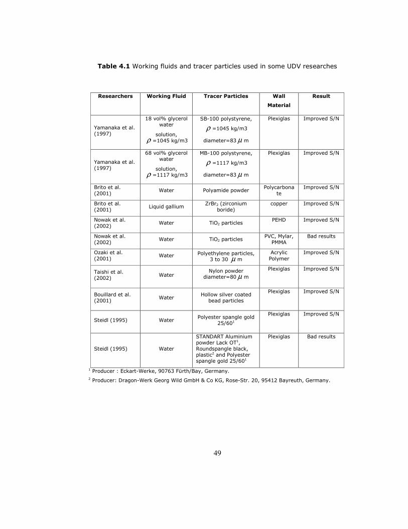
49
Table 4.1 Working fluids and tracer particles used in some UDV researches
Researchers Working Fluid Tracer Particles Wall
Material
Result
Yamanaka et al. (1997)
18 vol% glycerol water
solution, ρ =1045 kg/m3
SB-100 polystyrene,
ρ =1045 kg/m3
diameter=83 µ m
Plexiglas Improved S/N
Yamanaka et al. (1997)
68 vol% glycerol water
solution, ρ =1117 kg/m3
MB-100 polystyrene,
ρ =1117 kg/m3
diameter=83 µ m
Plexiglas Improved S/N
Brito et al. (2001)
Water Polyamide powder Polycarbona
te Improved S/N
Brito et al. (2001)
Liquid gallium ZrBr2 (zirconium
boride) copper Improved S/N
Nowak et al. (2002)
Water TiO2 particles PEHD Improved S/N
Nowak et al. (2002)
Water TiO2 particles PVC, Mylar,
PMMA Bad results
Ozaki et al. (2001)
Water Polyethylene particles, 3 to 30 µ m
Acrylic Polymer
Improved S/N
Taishi et al. (2002)
Water Nylon powder
diameter=80 µ m
Plexiglas Improved S/N
Bouillard et al. (2001)
Water Hollow silver coated
bead particles
Plexiglas Improved S/N
Steidl (1995) Water Polyester spangle gold
25/601
Plexiglas Improved S/N
Steidl (1995) Water
STANDART Aluminium powder Lack OT1, Roundspangle black, plastic2 and Polyester spangle gold 25/601
Plexiglas Bad results
1 Producer : Eckart-Werke, 90763 Fürth/Bay, Germany. 2 Producer: Dragon-Werk Georg Wild GmbH & Co KG, Rose-Str. 20, 95412 Bayreuth, Germany.

50
4.3. Lightsheet Experiments
Steidl (1995) performed laser light sheet experiments in order to investigate the
flow in a 400 mm length square tank qualitatively. He made trials with different
types of aluminium particles to determine the best particle for the visualization
of the flow field in the stirred tank. The following particle types were
investigated:
Table 4.2 Particle types for the laser-lightsheet (Steidl, 1995)
Particle type average corn size in
[µm]
STANDART Aluminium powder 1111 45
STANDART Aluminium powder Lack OT 80
STANDART Aluminium spangle fine 250
He found that the particles with a corn diameter of 80 µm were optimal for the
visualization of the flow in the tank. He stated that principally both other
particles can also be used in the experiments and finer particles are generally
more suitable for the visualization of fine structures of flow.
4.4. Aeration
Many models have been presented to predict gas–liquid mass transfer to/from
clean bubbles, i.e. bubbles with a mobile surface. Most of these models assume
that mass transfer is controlled by the rate of surface renewal, as described by

51
Higbie’s penetration theory (Higbie, 1935). According to this theory, the liquid-
phase mass transfer coefficient for a bubble with a mobile surface is given by
θπ
DkL
2= (3.4)
The problem with the application of Equation 3.4 lies in the calculation of the
surface renewal time θ . Two major approaches have been suggested, which
depend on the scale of flow that is assumed to influence mass transfer.
The first one, proposed by Higbie (1935), himself relates the contact time to the
bulk liquid flow around the bubble assuming that
u
d B=θ (3.5)
where d is the bubble diameter and u is the bubble slip velocity, leading to the
following equation:
2/113.1 D
d
uk
B
L = . (3.6)
An alternative approach starts from a refinement of Higbie’s theory by
Danckwerts (1951), who proposed that the average surface renewal rate results
from exposure to eddies with variable contact time, leading to Equation 3.7:
DskL = . (3.7)
Lamont and Scott (1970) calculated the fractional rate of surface-element
replacement, s, through an eddy cell model, postulating that mass transfer is
mainly dependent on the motion of small-scale eddies in the dissipation range of
the spectrum. They deduced that

52
4/1
2/1
=
υ
εcDkL (3.8)
where ε is the turbulent energy dissipation, υ is the kinematic viscosity and c
= 0.4 is a constant. Kawase et al. (1987) presented an alternative approach,
resorting to Kolmogoroff’s theory of isotropic turbulence, valid for power-law
liquids. This leads to Equation 3.8 above for the particular case of Newtonian
liquids, with constant c = 1.13. Prasher and Wills (1973) obtained c = 0.592
from experimental data in a stirred tank. The major differences between
Equations 3.6 and 3.8 are that equation 3.6 predicts an important variation in kL
with diameter, excluding turbulence as an independent variable, whereas
equation 3.8 predicts a decisive influence of turbulent energy dissipation on kL,
making it independent of bubble diameter (Alves et al, 2005).
Calderbank et al. (1960) had developed techniques for measuring the interfacial
area in gas-liquid dispersions and consequently made it possible to measure the
liquid phase mass transfer coefficients in gas-liquid dispersions such as are
produced in aerated mixing vessels, and sieve and sintered plate columns.
Nagata (1975) states that Calderbank has observed the interfacial area of air in
agitated water by a light transmission technique. In a mixing vessel agitated in
100-400 rpm under aeration AQ = 1 ft3/min, there are two maxima of interfacial
are in the vicinity of an impeller and in the middle height between the impeller
and the free surface.
Chisti et al. (2001) has investigated the gas holdup, mixing, liquid circulation
and gas–liquid oxygen transfer characterized in a large (~1.5m3) draft-tube
airlift bioreactoragitated with Prochem® hydrofoil impellers placed in the draft-
tube. They made measurements both in water and in cellulose fiber slurries.
They found that the use of mechanical agitation generally enhanced mixing
performance and the oxygen transfer capability relative to when mechanical
agitation was not used; however, the oxygen transfer efficiency was reduced by
mechanical agitation.

53
Kawase et al. (1986) developed a theoretical model for volumetric mass transfer
coefficients in bubble columns which was based on Higbie’s penetration theory
and Kolmogoroff's theory of isotropic turbulence.
As explained in Chapter 2, according to the theory of Higbie (Higbie, 1935) there
is a relationship between the residence time of the fluid particles at the interface
and the oxygen transfer coefficient. The residence time of the fluid bubbles is
depended on the bubble surface consequently on the size of the bubble.
Experimental researches of this dependency have been done by Motarjemi
(1978), Pasveer (1955) and Bishof (1994).

54
CHAPTER V
EXPERIMENTAL WORK
5.1. Set-up of Cylindrical Tank Experiments
The experimental set-up is shown in Figure 5.1. It is mainly composed of a
mixing tank, a rotating impeller, a conductivity electrode, torquemeter and a PC
whose details are given below.
Figure 5.1 Experimental Set-up for Mixing Time Experiments
Conductivity Electrode
n H
PC
d
Baffles
Impeller
Tracer Injection
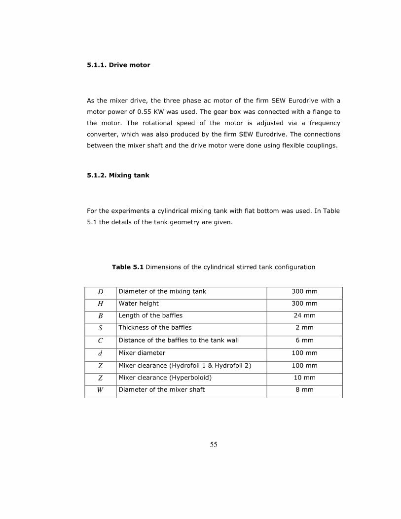
55
5.1.1. Drive motor
As the mixer drive, the three phase ac motor of the firm SEW Eurodrive with a
motor power of 0.55 KW was used. The gear box was connected with a flange to
the motor. The rotational speed of the motor is adjusted via a frequency
converter, which was also produced by the firm SEW Eurodrive. The connections
between the mixer shaft and the drive motor were done using flexible couplings.
5.1.2. Mixing tank
For the experiments a cylindrical mixing tank with flat bottom was used. In Table
5.1 the details of the tank geometry are given.
Table 5.1 Dimensions of the cylindrical stirred tank configuration
D Diameter of the mixing tank 300 mm
H Water height 300 mm
B Length of the baffles 24 mm
S Thickness of the baffles 2 mm
C Distance of the baffles to the tank wall 6 mm
d Mixer diameter 100 mm
Z Mixer clearance (Hydrofoil 1 & Hydrofoil 2) 100 mm
Z Mixer clearance (Hyperboloid) 10 mm
W Diameter of the mixer shaft 8 mm

56
Hyperboloid impeller which had been designed as a close clearance impeller was
placed at a clearance of 10 mm ( 10/dZ = ) from the tank bottom. In the
hydrofoil 1 and hyperboloid impeller combination, the hyperboloid mixer was
placed at a clearance of 10 mm ( 10/dZ = ) from the tank bottom and the
hydrofoil1 impeller which is on the same shaft was placed 100 mm ( d ) lower
than the water surface. The baffles were located in the stirred tank with 90°
angle (see Figure 5.2).
Figure 5.2 Stirred tank configuration
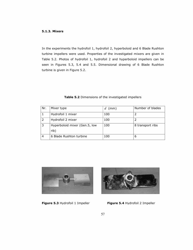
57
5.1.3. Mixers
In the experiments the hydrofoil 1, hydrofoil 2, hyperboloid and 6 Blade Rushton
turbine impellers were used. Properties of the investigated mixers are given in
Table 5.2. Photos of hydrofoil 1, hydrofoil 2 and hyperboloid impellers can be
seen in Figures 5.3, 5.4 and 5.5. Dimensional drawing of 6 Blade Rushton
turbine is given in Figure 5.2.
Table 5.2 Dimensions of the investigated impellers
Nr. Mixer type d (mm) Number of blades
1 Hydrofoil 1 mixer 100 2
2 Hydrofoil 2 mixer 100 2
3 Hyperboloid mixer (Gen.5, low
rib)
100 8 transport ribs
4 6 Blade Rushton turbine 100 6
Figure 5.3 Hydrofoil 1 Impeller Figure 5.4 Hydrofoil 2 Impeller

58
Figure 5.5 Hyperboloid Impeller
Specifications of hydrofoil1 impeller is given in Table 5.3.
Table 5.3 Specifications of hydrofoil 1 impeller
D = 300 mm
Profile form 417 A
Diameter 100 mm D333.0
Number of blades 2 -
Blade angle 15° -
bladel 33 mm d33.0
bladeb 33 mm d33.0
bladew 0.7 mm d007.0
hubd 15 mm D05.0
hubh 15 mm D05.0
W 8 mm D027.0
The available specifications of Hydrofoil 2 impeller is given in Table 5.4.
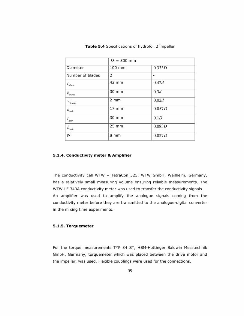
59
Table 5.4 Specifications of hydrofoil 2 impeller
D = 300 mm
Diameter 100 mm D333.0
Number of blades 2 -
bladel 42 mm d42.0
bladeb 30 mm d3.0
bladew 2 mm d02.0
hubb 17 mm D057.0
hubl 30 mm D1.0
hubh 25 mm D083.0
W 8 mm D027.0
5.1.4. Conductivity meter & Amplifier
The conductivity cell WTW – TetraCon 325, WTW GmbH, Weilheim, Germany,
has a relatively small measuring volume ensuring reliable measurements. The
WTW-LF 340A conductivity meter was used to transfer the conductivity signals.
An amplifier was used to amplify the analogue signals coming from the
conductivity meter before they are transmitted to the analogue-digital converter
in the mixing time experiments.
5.1.5. Torquemeter
For the torque measurements TYP 34 ST, HBM-Hottinger Baldwin Messtechnik
GmbH, Germany, torquemeter which was placed between the drive motor and
the impeller, was used. Flexible couplings were used for the connections.

60
5.1.6. Ultrasound Doppler Velocimeter
The measurements were performed with the UDV system (Met-Flow SA,
Switzerland), which allows the measurement of the fluid velocity at 128 points
along the beam direction. By using the Ultrasound Doppler Velocimeter one can
measure a complete velocity profile along the direction of the probe in a few
seconds.
At each measurement cycle of the device 1024 profiles are taken, the data of
which can be further saved to a floppy. The device works with a main frequency
of 4 MHz and the diameter of the focused ultrasound beams were 5 mm. The
thickness of the measurement volumes depends on the sound velocity of the
investigated fluid and the value for water is 0.75 mm. Four different ultrasonic
beam lengths can be set by the device itself where certain limitations exist
regarding the maximum measurable velocities or the resolution of the velocity
values. These are given in Table 5.3 for water ( c =1480 m/s).
Table 5.5 Depths and the maximum measurable velocities in UDV system.
Maximum Depth Maximum Velocity Resolution
91 [mm] 722 [mm/s] 5.6 [mm/s]
189 [mm] 361 [mm/s] 2.8 [mm/s]
378 [mm] 181 [mm/s] 1.4 [mm/s]
758 [mm] 90 [mm/s] 0.7 [mm/s]

61
5.2. Experimental Procedures for Cylindrical Tank Experiments
5.2.1. Power Consumption Measurements
Torque versus impeller rotational speed measurements were done for the
impellers hydrofoil 1, hydrofoil 2, hyperboloid and a combination of the
hyperboloid and the hydrofoil 1 impeller using water as the working fluid.
In order to obtain the torque data at a certain rotational speed, the mixers were
first rotated in air, and the torque on the mixer shaft was measured for each
rotational speed. Then, the system was operated with water and the torque data
were recorded again at the same rotational speeds. The torque data obtained for
air were further subtracted from the torque data obtained for water to get the
final torque data.
A simple calculation was carried out to obtain the Newton Number from the
torque data.
First the Power in Watts was obtained from the torque data;
ωTP = (5.1)
nπω 2= (5.2)
53 *** dnNeP ρ= (5.3)
where P is power in Watts, T is torque in N.m and n is the rotational speed in
RPS and Ne is the dimensionless Newton Number.
A sample calculation is carried out with raw data of the hydrofoil 1 impeller
according to the above given formulas. (See Appendix E) Torque was

62
measured as 04.0=T Nm for hydrofoil 1 impeller at a rotational speed of
783 RPM. Under this conditions Re , Ne and P were calculated as 130505,
0.15 and 3.28 Watt, respectively. Using this procedure the Ne−Re curves for
the three mixers were constructed.
5.2.2. Macromixing Time Measurements
5.2.2.1. Measurement Procedure
The procedure used in the experiments was based on monitoring concentration
change of a tracer with respect to time at a fixed point. An electrolyte substance
was added as the tracer to the vessel. The concentration of this substance was
measured by a conductivity meter. The 95 % mixing time was determined from
the changes in conductivity after introducing 21 ml (0.1 % of the tank volume)
of aqueous sodium chloride solution (10 w/w %) to the free surface of the liquid
near the mixer shaft.
The conductivity recording was always started at the same time with the addition
of the salt solution and until one or two minutes after the injection depending on
the stirrer studied, so that steady concentration versus time behavior is
obtained. The conductivity electrode was located inside the vessel, so that the
conductivity cell was approximately at the midpoint of the liquid height and in
the middle between the shaft and the vessel wall.
Before starting the measurements, it was necessary to calibrate the conductivity
cell against the possibility that the relative concentration fluctuations less than 5
% of the middle value could be resolved and the maximum limit value of the
electrolyte concentration was kept until the time when a proportional relationship
between the concentration and the conductivity was achieved.
63
The conductivity signal coming from the conductivity cell was transferred
through the conductivity meter, the amplifier and an analogue-digital converter
to the PC, where the data was recorded.
To ensure a sufficient statistical safety in the results, the average of a number of
measurements must be taken. For the same operating conditions the mixing
time was calculated six times and they were averaged after eliminating the
maximum and minimum values.
At each measurement the beginning and the end concentrations were recorded
for 16 seconds and the mixing period was recorded for 65 seconds. The
recording was done for every 10 milliseconds.
A calibration curve is required to convert the conductivity data in Volts to the
concentration data. NaCl solutions at different concentrations (mmol/l) were
prepared with deionized water. The conductivities of these solutions were
measured. The care was taken for the water temperature in the foregoing
experiments to be the same with that of the calibration experiments. Average of
two measurements was considered for each concentration
There exists a lag time for the conductivity meter to display the conductivity
value when the probe is inserted into the solution. The lag time for the
conductivity probe was determined by measuring the time lost from the moment
where the probe is inserted into the solution until the conductivity value appears
on the conductivity meter. For the measurement the stop watch is started
simultaneously with the insertion of the probe into the solution. The lag time is
usually about 2-3 seconds. The lag time of the conductivity meter was measured
as 2.1 s.
5.2.2.2. Macro Mixing Time Calculation Procedure
The conductivity versus time data were stored in computer and were further
evaluated to get the mixing time via the prepared Excel sheet. First the
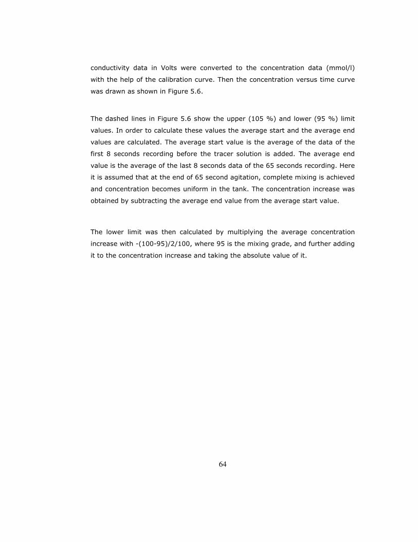
64
conductivity data in Volts were converted to the concentration data (mmol/l)
with the help of the calibration curve. Then the concentration versus time curve
was drawn as shown in Figure 5.6.
The dashed lines in Figure 5.6 show the upper (105 %) and lower (95 %) limit
values. In order to calculate these values the average start and the average end
values are calculated. The average start value is the average of the data of the
first 8 seconds recording before the tracer solution is added. The average end
value is the average of the last 8 seconds data of the 65 seconds recording. Here
it is assumed that at the end of 65 second agitation, complete mixing is achieved
and concentration becomes uniform in the tank. The concentration increase was
obtained by subtracting the average end value from the average start value.
The lower limit was then calculated by multiplying the average concentration
increase with -(100-95)/2/100, where 95 is the mixing grade, and further adding
it to the concentration increase and taking the absolute value of it.
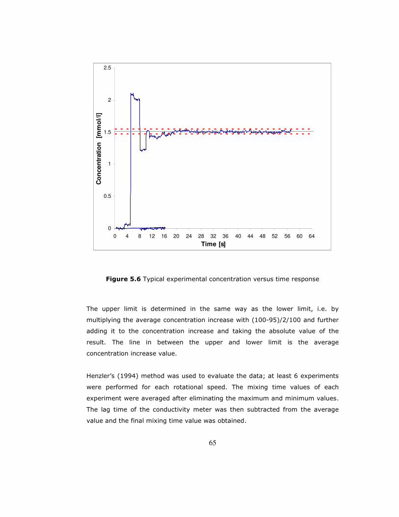
65
0
0.5
1
1.5
2
2.5
0 4 8 12 16 20 24 28 32 36 40 44 48 52 56 60 64
Time [s]
Co
ncen
trati
on
[m
mo
l/l]
Figure 5.6 Typical experimental concentration versus time response
The upper limit is determined in the same way as the lower limit, i.e. by
multiplying the average concentration increase with (100-95)/2/100 and further
adding it to the concentration increase and taking the absolute value of the
result. The line in between the upper and lower limit is the average
concentration increase value.
Henzler’s (1994) method was used to evaluate the data; at least 6 experiments
were performed for each rotational speed. The mixing time values of each
experiment were averaged after eliminating the maximum and minimum values.
The lag time of the conductivity meter was then subtracted from the average
value and the final mixing time value was obtained.
66
5.2.3. Ultrasound Doppler Velocimeter Measurements
Polyesterspangle 25/60 gold (Regular hexagon, Edge length 0.60 mm, Height
0.25 mm) particles were used as scatterers in the experiments. The tank wall
was made of glass. The thickness of the wall was 4 mm. The sound speed of
water was taken as 1480 m/s which was also the set value of the device. In the
experiments axial and radial measurements were performed. 5 measurements
were done for each measuring point. The rotational speeds of the impellers were
adjusted to 382 RPM (Re=63666), which corresponds to 2 m/s tip speed.
Axial Measurements
The measurements in the axial plane were done as shown in Figure 5.7. The
UDV probe head was located downwards at a certain height from the liquid
surface. By installing the probe at different radii a whole plane of the axial
velocity can be measured. (Steidl, 1995) In the experiments the measurements
were taken with 1 cm spacing in between the mixer shaft and the tank wall at
the set axial heights.

67
Figure 5.7 Axial UDA measurements
Radial Measurements
The measurement of radial velocity profiles is similar to the measurement of the
axial planes. In this case the sensor can be placed horizontally either outside or
inside the vessel. (Steidl, 1995) In the experiments the probe was fixed on the
outside of the mixing tank via a plexiglas wall having holes on it and attached to
the one side of the mixing tank. The probe was placed on the holes depending
on the location at which measurement was required. Ultrasonic gel was used as
the coupling medium. A representative picture can be seen in Figure 5.8.
68
Figure 5.8 Radial UDV measurements
5.2.3.1. Calculation Procedure for the UDV Measurements
For the evaluation of the binary data recorded by the UDV Monitor, the UVP
Graph program developed by Steidl (1995) was used. The outputs of the UVP
Graph program were further sent to the supplementary programs DrawStr
(Steidl, 1995) and Dat2Tec (Steidl, 1995), which prepared data for the TecPlot
to display the stirred tank and the velocities in x and y direction.

69
Figure 5.9 Evaluation process of the UDV data
5.2.4. Lightsheet Experiments
A test set-up has been built to record flow images of the investigated impellers
by means of light sheet technique. The mixing tank was covered with black
paper. Light coming from a 1000 watt light source was sent through a 4 mm
rectangular hole which was made on the black paper covering the left side of the
tank. The centerline of the hole was exactly the center of the tank in the
direction of the mixer shaft in between two baffles. The previously added
aluminum particles become shiny along the center of the mixing tank when the
light source was activated. So, the flow field on the left side of the tank
generated by the mixers could be visualized as long as the laboratory medium is
kept dark. The Reynolds numbers studied were 118114 and 81254. The
UDV System
Rawdata in binary form
uvpgraph
Measured values in ASCII form
Dat2Tec DrawStr
Mixer Geometry
preplot
tecplot Coloured Printer
preplot
Single velocity profiles to one plane

70
aluminum particles used in the experiment was of type Standard Aluminium
Powder, Lack OT Ch., Eckart Werke D-90763 Fürth, Germany. The diameter of
aluminum particles were 80 µ m. Small spoonful aluminium particles were
enough to obtain a satisfactory visualization. For the aluminium particles to have
a uniform distribution in water, a small amount of liquid soap was required to be
added to it.
After turning on the light and starting up the mixer, the flow in the tank was
recorded by the Sony Digital Video Camera Recorder, DCR-VX1000E. To obtain a
satisfactory result in the flow visualization, main parameter to be adjusted in the
camera settings was the shutter speed. The shutter time can be arranged from
1/3 to 1/10000. With higher shutter time the amount of light the camera lets in
itself is higher and with a higher light the flow could be visualized more clearly.
Adjusting a high shutter time is a must in the lightsheet experiments, since the
medium is dark except the light sheet sent into the tank. In the experiment the
recordings were done with the shutter times 1/3, 1/6, 1/12 and 1/25 s.
In the experiments working long time with the same water was a disadvantage.
The aluminum particles got dissolved in water and disabled the visualization of
the flow field. It is better to change the water in the tank before each recording.
Another disadvantage was using more than one spoonful of particles. This also
prevented a clear visualization of the flow field. Both of these disadvantages had
been experienced in the lightsheet experiments of the combination 2
(submergence of the top hydrofoil impeller = 1.5 d ) case.
5.3. Square Tank Experiments
Conductivity and aeration measurements were performed with different types of
mixers in the square tank which is a geometry extensively used in waste water
treatment. The drive motor used was of the firm MATTKE Antriebstechnik with a

71
maximum torque capacity of 32 Nm. The dimensions of the square Plexiglas
mixing tank were 900x900 mm. The details of the tank configuration are given in
Table 5.4.
Table 5.6 Dimensions of the rectangular stirred tank
l Tank length 900 mm
w Tank width 900 mm
H Water height 450 mm
d Mixer diameter 200 mm
Z Mixer clearances 20 mm
W Diameter of the conical mixer shaft 20 mm (upper part)
10 mm (lower part)
5.3.1. Mixers
In the experiments Generation 6 Hyperboloid, Generation 5 Hyperboloid (low rib)
and Generation 5 Hyperboloid (high rib) mixers were used.
The properties of the mixers are given in Table 5.9. The photos of the mixers are
shown in Figures 5.10-11-12.
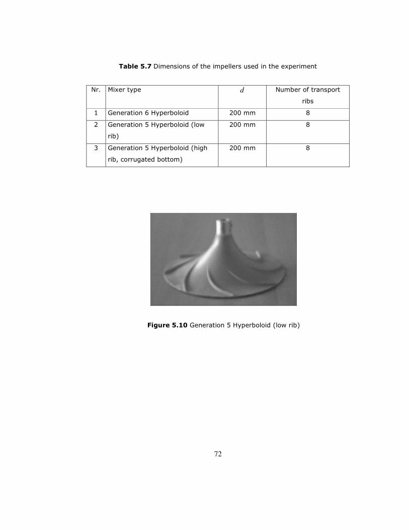
72
Table 5.7 Dimensions of the impellers used in the experiment
Nr. Mixer type d Number of transport
ribs
1 Generation 6 Hyperboloid 200 mm 8
2 Generation 5 Hyperboloid (low
rib)
200 mm 8
3 Generation 5 Hyperboloid (high
rib, corrugated bottom)
200 mm 8
Figure 5.10 Generation 5 Hyperboloid (low rib)

73
Figure 5.11 Generation 5 Hyperboloid (high rib)
Figure 5.12 Generation 6 Hyperboloid (front and bottom view)
5.3.2. Determination of the macromixing time
The same experimental procedure explained in part 5.1 with the required scale-
up was employed in the experiment.
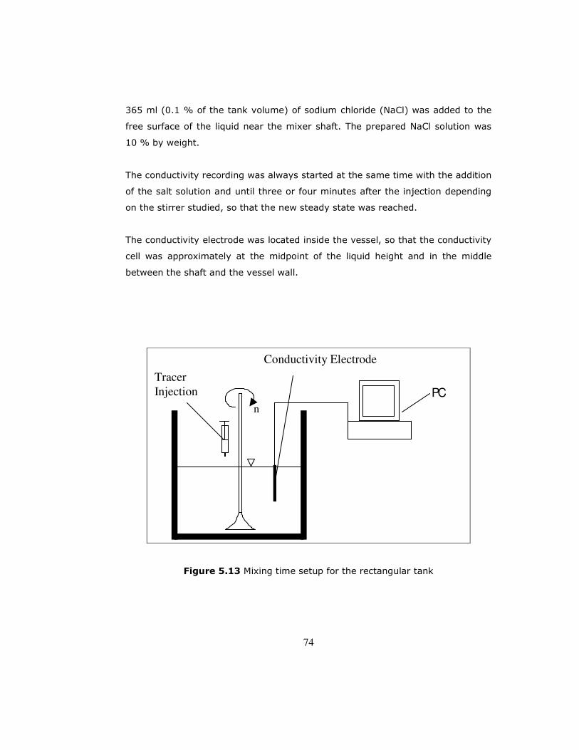
74
365 ml (0.1 % of the tank volume) of sodium chloride (NaCl) was added to the
free surface of the liquid near the mixer shaft. The prepared NaCl solution was
10 % by weight.
The conductivity recording was always started at the same time with the addition
of the salt solution and until three or four minutes after the injection depending
on the stirrer studied, so that the new steady state was reached.
The conductivity electrode was located inside the vessel, so that the conductivity
cell was approximately at the midpoint of the liquid height and in the middle
between the shaft and the vessel wall.
n
Tracer
Injection
Conductivity Electrode
PC
Figure 5.13 Mixing time setup for the rectangular tank
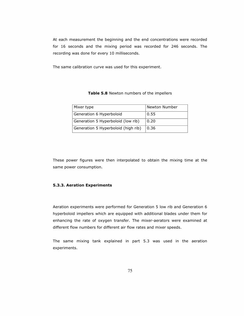
75
At each measurement the beginning and the end concentrations were recorded
for 16 seconds and the mixing period was recorded for 246 seconds. The
recording was done for every 10 milliseconds.
The same calibration curve was used for this experiment.
Table 5.8 Newton numbers of the impellers
Mixer type Newton Number
Generation 6 Hyperboloid 0.55
Generation 5 Hyperboloid (low rib) 0.20
Generation 5 Hyperboloid (high rib) 0.36
These power figures were then interpolated to obtain the mixing time at the
same power consumption.
5.3.3. Aeration Experiments
Aeration experiments were performed for Generation 5 low rib and Generation 6
hyperboloid impellers which are equipped with additional blades under them for
enhancing the rate of oxygen transfer. The mixer-aerators were examined at
different flow numbers for different air flow rates and mixer speeds.
The same mixing tank explained in part 5.3 was used in the aeration
experiments.

76
There was an aeration ring under the mixer where the air was pumped to the
system. The velocity and air flow rate were adjusted with the buttons on the
panel which was at the right side of the tank.
Generation 5 low rib mixer which had blades under it is given in Figure 5.14.
These blades were used for aeration purposes; to make the air bubbles smaller
and consequently to increase the interfacial area between air and solution. The
mixer clearance was 32 mm, which was 20 mm in the conductivity experiments,
to account for the aeration ring.
Figure 5.14 Front view of the mixer aerator
Oxygen-meter and Oxygen Sensor
The oxygen-meter and the oxygen sensor, model Cond 340i, of the Firm WTW
(Germany) were used to determine the oxygen concentration in the tank. The

77
oxygen sensor was always placed at the front left corner of the tank. In order to
determine the oxygen transfer coefficient, the oxygen entry to the system with
respect to time is obtained in the form of a concentration curve with the help of
the data collected by the oxygen electrodes. The procedure followed for the
measurement of the oxygen transfer in clean water was the one “Absorption
measurements following the lowering of the DO concentration using sodium
sulphite” explained in the advisory leaflet ATV M 209 (1996). Detailed
description of the procedure is given in Appendix E.
78
CHAPTER VI
RESULTS AND DISCUSSION
6.1. Cylindrical Tank Results
6.1.1. Power Consumption
Newton number and mixing time are two important parameters for evaluating
the efficiency of impellers. Newton (power) number, Ne, is a dimensionless
parameter which measures the power requirements of an impeller. Correlations
for Ne as a function of Reynolds Number are available in literature. A good
impeller is the one that has a small mixing time as well as a small power
number.
Power characteristics of the impellers were investigated in the fully developed
turbulent region at Re >40000. The measured torque versus rotational speed
data were converted to dimensionless Reynolds and Newton number data. The
power consumption characteristics of the investigated impellers and impeller
combinations are given in Figure 6.1. Newton numbers of the impellers turned
out to be constant at Re >130000 consequently at this range Newton Numbers
were averaged to obtain the turbulent Newton numbers of the impellers. The
highest Newton number, 0.60, was that of the Hydrofoil 1+Hyperboloid impeller
combination’s with the top impeller (hydrofoil 1) submergence of 1.5 d .
Hydrofoil 1 impeller had the lowest Newton number, which was 0.15.
79
Two different hydrofoil impellers were investigated, the Newton number of
hydrofoil 1 impeller (0.15) were found to be lower than the new design hydrofoil
2 impeller (0.32).
Schäfer (2001) worked with a profile 417 A hydrofoil impeller which has nearly
the same geometry with the hydrofoil 1 impeller investigated in this study. He
found the Newton number as 0.145 for a Dd / ratio of 0.375 while the Dd /
ratio in this study is 0.333 and the found Newton Number is 0.15. He stated that
this value was lower by a factor of 10-30 compared to other standard impellers’
Newton numbers. Fentiman et al. (1998) also worked with a hydrofoil impeller
and found the Newton number as 0.22.
The Newton number of the hyperboloid impeller (0.39) was found to be higher
than that of the two hydrofoil impellers. It will be seen that the Newton numbers
of the radial flow producing impellers are higher than that of the axial flow
producing impellers in each case when the published literature is examined.
Higher Newton number of the radial flow producing hyperboloid impeller than
that of the axial flow producing hydrofoil impellers’ can be due to this difference.
The Newton numbers of the two impeller combinations were found to be higher
than the single impeller combinations as expected. Among the two impeller
combinations the Hydrofoil 1+Hyperboloid impeller combination with the top
impeller (hydrofoil 1) submergence of 1.5 d has a Newton Number of 0.60 while
the combination with the top impeller (hydrofoil 1) submergence of d has a
Newton Number of 0.55. Nere et al. (2003) have stated that the impeller off-
bottom clearance plays an important role in the overall flow pattern generated
by an impeller and also affects the power consumption. Rao et al. (1988) have
investigated the Newton Numbers of axial-downflow pitched blade turbines and
have found that as the impeller off-bottom clearance decreases the Newton
Number increases; at 3/DZ = Ne =1.29, at 4/DZ = Ne =1.35 and at
6/DZ = Ne=1.61. The difference between the Newton numbers of the two
mixer combinations might be due to the decrease in the axial flow producing

80
upper m
ixer off-bottom
clearance as in
the case for R
ao et al. (1
988). T
he raw
data of th
e pow
er consu
mptio
n m
easurem
ents in
cylindrical tan
k are given
in
Appen
dix A
.
0.00
0.20
0.40
0.60
0.80
1.00
1.20
1.40
1.60
0 20000 40000 60000 80000 100000 120000 140000 160000 180000
Re [-]
Ne [-]
Hydrofoil 1 Ne=0.15 Hydrofoil 2 Ne=0.32Hyperboloid Ne=0.39 Hydrofoil1+Hyperboloid (d) Ne=0.55Hydrofoil1+Hyperboloid (1.5d) Ne=0.60
Figure 6.1 Power characterisitics of the investigated impellers

81
6.1.2. Macromixing Measurements
Because of the availability of the literature data the reliability of the macromixing
measurements was first checked with the results of the 6-blade Rushton turbine
experiments. Results of the macromixing experiments performed with the 6-
blade Rushton turbine impeller checked with the data reported by Zlokarnik
(1998). The results are depicted in Figure 6.2 along with the literature values.
0
10
20
30
40
50
60
0 20000 40000 60000 80000 100000 120000
Re
n*teta
ExperimentalLiteraturePower (Experimental)
Figure 6.2 Mixing time characteristics for the 6 blade Rushton turbine
82
In Figure 6.2, y axis represents the dimensionless mixing time number, θn .
Both results levels off approximately at 35 in the fully turbulent region. Despite
the slight differences between the results, the employed mixing time
measurement method was considered accurate enough to be used in the
following stages of this study.
In Figure 6.3 the dimensionless macromixing time versus Reynolds number
graph for the investigated impellers are shown. The dimensionless mixing time
numbers have been obtained for a dimensionless mixing grade of M=0.95.
Dimensionless times remain almost constant for each impeller type as opposed
to the dimensional time. Therefore it should be the number of turns, not time
itself, which affects the degree of mixing. Since Figure 6.3 is in terms of
dimensionless numbers, it is universally applicable for the respective tank and
impeller geometries. The dimensionless mixing time numbers of the impellers
are given in Table 6.1. Rushton turbine has the lowest (38.70) and the
hyperboloid impeller has the highest (177.92) dimensionless mixing time.
In Figure 6.4, variation of macromixing time with the rotational speed is given.
As expected dimensional mixing time decreases sharply with increasing
rotational impeller speed followed by a nearly constant mixing times at high
rotational speeds. This behavior was exhibited by all impellers and impeller
combinations although their quantitative responses were considerably different
as given in Table 6.2.
As also stated earlier the most efficient impeller is the one with lowest Newton
Number as well as the lowest dimensionless mixing time. The comparison
between the impellers was done by determining their mixing times on the basis
of equal power consumption. The power consumption of one of the mixers, i.e.
hydrofoil 1, was selected as basis. Then the mixing time and the rotational speed
values of the other mixers corresponding to the same power consumption were
found by interpolation. At the same specific power consumption hydrofoil 1
impeller had the shortest mixing time, 7.81, whereas the hyperboloid impeller
had the highest mixing time, 19.20.
83
In their review Nere et al. (2003) have mentioned about Rutherford et al.’s
study, which was focused on the effect of blade thickness; Rutherford et al. have
investigated the effect of the blade (bladew ) thickness on the flow and power
numbers. They found that the flow number, power number, fluctuating velocity,
and average velocity were higher for thinner impellers. Hence they observed
lower mixing times for thinner impellers. With comparison on an equal power
consumption basis, the mixing time was found to lower by 13% for the thinner
impeller compared to the thicker radial flow impeller (Nere et al., 2003).
Hydrofoil 1 impeller is better in mixing efficiency compared to hydrofoil 2
impeller, this might be due to the blade thickness of hydrofoil 2 impeller which is
about three times larger than that of the the hydrofoil 1 impeller.
Hydrofoil 1 impeller proved to be the best in macromixing efficiency among the
investigated impellers, this is due to the higher discharge flow produced by the
hydrofoil 1 impeller compared to other impellers at equal power consumption;
the study of Fentiman et al. (1998) regarding the characteristics of a hydrofoil
impeller has been given in part 4.1.1. Distelhoff et al.’s study, as explained in
part 4.1.1, also indicates that axial flow impellers have shorter mixing times
compared to the radial ones at equal power consumption.
Hydrofoil mixers provide strong axial top to bottom flow all over the mixing tank,
however hyperboloid mixers provide a radial flow especially in the tank bottom
and a slower mixing occurs in the upper part of the mixing tank. The high mixing
time value of hyperboloid mixer can be attributed to this, since in the
experiments the salt solution is added from the surface of the mixing tank.
Because of that the hyperboloid impeller is effective in the lower part of the
tank; the upper part of the mixing tank might have not been mobilized as much
as the lower part of the tank.
In selecting impeller type another important criteria is the physical nature of the
material to be agitated or mixed. Appropriate configuration should be used
depending on the solution viscosity, density, and multi-phase characteristics, i.e.
if the solution to be treated is a suspension, emulsion or gas-liquid mixture. The

84
hyperboloid impellers were developed for suspension and dispersion purposes.
Because of their design as close clearance impellers, they do not have good
macromixing properties compared to standard impellers. The flow a hyperboloid
produce goes radially over the tank bottom reach the tank wall and return back
to the mixer top axially. This prevents the settling of heavy particles in the tank
bottom, makes them get mobilized and also provides a good dispersion in
aeration.
Considering the aforementioned characteristics of the hyperboloid mixer, a mixer
combination of it, especially with an impeller having a high pumping capacity, is
a reasonable choice for waste water treatment facilities since the bottom
circulation produced by the hyperboloid mixer would be distributed along the
whole tank and a complete top to bottom circulation will be achieved. Two
different combinations of hyperboloid impeller with hydrofoil 1 impeller were
used for this purpose in this study.
When the two hydrofoil 1 and hyperboloid impeller combinations are compared
the one having the upper mixer off-surface clearance of d, in which the upper
mixer is closer to the water surface, proved to be more efficient. This is an
expected result; in the literature various studies indicate that the mixing time
increases with a decrease in the off-bottom clearance of the axial flow impeller.
Rao et al.’s (1988) study , which was explained in Part 6.1.1, have shown that
for the axial flow producing downflow pitched blade turbine the value of the
mixing time was found to increase with a decrease in the impeller clearance.
The raw data of the macromixing measurements in cylindrical tank are given in
Appendix B.
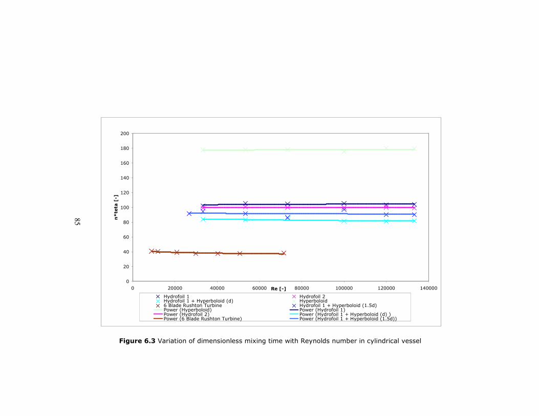
85
0
20
40
60
80
100
120
140
160
180
200
0 20000 40000 60000 80000 100000 120000 140000Re [-]
n*teta [-]
Hydrofoil 1 Hydrofoil 2Hydrofoil 1 + Hyperboloid (d) Hyperboloid6 Blade Rushton Turbine Hydrofoil 1 + Hyperboloid (1.5d)Power (Hyperboloid) Power (Hydrofoil 1)Power (Hydrofoil 2) Power (Hydrofoil 1 + Hyperboloid (d) )Power (6 Blade Rushton Turbine) Power (Hydrofoil 1 + Hyperboloid (1.5d))
Figure 6.3 Variation of dimensionless mixing time with Reynolds number in cylindrical vessel
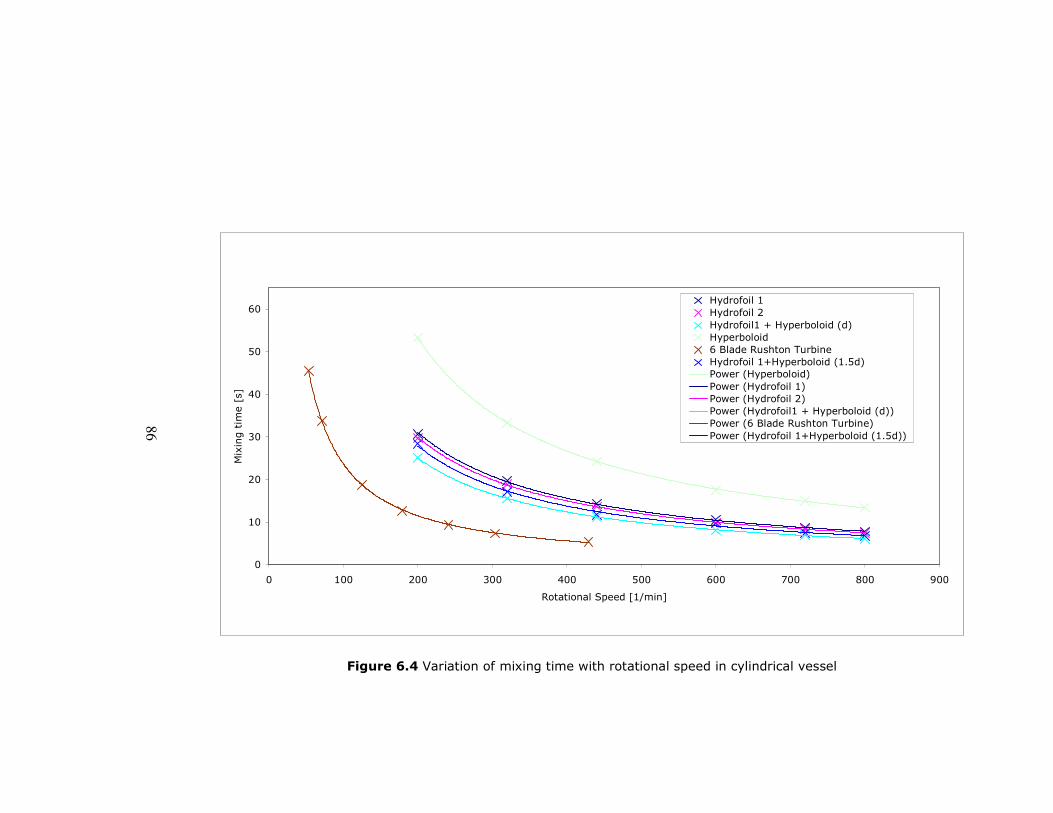
86
0
10
20
30
40
50
60
0 100 200 300 400 500 600 700 800 900
Rotational Speed [1/min]
Mix
ing tim
e [s]
Hydrofoil 1Hydrofoil 2Hydrofoil1 + Hyperboloid (d)Hyperboloid6 Blade Rushton TurbineHydrofoil 1+Hyperboloid (1.5d)Power (Hyperboloid)Power (Hydrofoil 1)Power (Hydrofoil 2)Power (Hydrofoil1 + Hyperboloid (d))Power (6 Blade Rushton Turbine)Power (Hydrofoil 1+Hyperboloid (1.5d))
Figure 6.4 Variation of mixing time with rotational speed in cylindrical vessel

87
Table 6.1 Dimensionless mixing time numbers of the investigated impellers
Impeller Type θn
Rushton Turbine 38.70
Hydrofoil 1 Impeller 104.2
Hydrofoil 2 Impeller 99.84
Hyperboloid Impeller 177.92
Hydrofoil 1 + Hyberboloid
Combination (1.5d)*
91.61
Hydrofoil 1 + Hyberboloid
Combination (d)
82.47
(*)Submergence of the top impeller (hydrofoil 1)
Table 6.2 Mixing times at the same power consumption for the investigated
impellers
VP / [W/m3] θ⋅n [-] n [1/s] θ [s]
Hydrofoil 1
Impeller 163 103.9 13.3
7.81
Hydrofoil 2
Impeller 163 100.59 10.5
9.58
Hyperboloid
Impeller 163 178.6 9.3
19.20
Hydrofoil 1 &
Hyperboloid
Combination
(d)*
163 83.08 8.3 10.01
Hydrofoil 1&
Hyperboloid
Combination
(1.5d)*
163 86.33 7.31 11.81
* Submergence of the top impeller (hydrofoil 1)
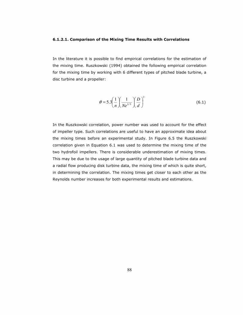
88
6.1.2.1. Comparison of the Mixing Time Results with Correlations
In the literature it is possible to find empirical correlations for the estimation of
the mixing time. Ruszkowski (1994) obtained the following empirical correlation
for the mixing time by working with 6 different types of pitched blade turbine, a
disc turbine and a propeller:
2
3/1
113.5
=
d
D
Nenθ (6.1)
In the Ruszkowski correlation, power number was used to account for the effect
of impeller type. Such correlations are useful to have an approximate idea about
the mixing times before an experimental study. In Figure 6.5 the Ruszkowski
correlation given in Equation 6.1 was used to determine the mixing time of the
two hydrofoil impellers. There is considerable underestimation of mixing times.
This may be due to the usage of large quantity of pitched blade turbine data and
a radial flow producing disk turbine data, the mixing time of which is quite short,
in determining the correlation. The mixing times get closer to each other as the
Reynolds number increases for both experimental results and estimations.
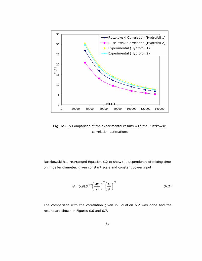
89
0
5
10
15
20
25
30
35
0 20000 40000 60000 80000 100000 120000 140000
Re [-]
t [s]
Ruszkowski Correlation (Hydrofoil 1)
Ruszkowski Correlation (Hydrofoil 2)
Experimental (Hydrofoil 1)
Experimental (Hydrofoil 2)
Figure 6.5 Comparison of the experimental results with the Ruszkowski
correlation estimations
Ruszkowski had rearranged Equation 6.2 to show the dependency of mixing time
on impeller diameter, given constant scale and constant power input:
3/13/1
3/291.5
=Θ
d
D
P
VD
ρ (6.2)
The comparison with the correlation given in Equation 6.2 was done and the
results are shown in Figures 6.6 and 6.7.

90
Further correlations for the estimation of macromixing time, e.g. Mersmann
(1994) and Corssin (1968), have been summarized in Nere et al.’s (2003)
overview.
As explained in part 3.1.1. Schäfer (2001) has also studied the macromixing
efficiency of a hydrofoil impeller which has also the profile form 417 A with d/D
ratio of 0.375. He stated that an estimation of macromixing efficiency through
Ruszkowski’s correlation wasn’t possible then on for hydrofoil impellers since the
estimation of mixing time was about 25% higher than his experimental results.
When Figure 6.6 is examined, it will be seen that the hydrofoil 1 impeller results
are in good agreement with Equation 6.2. Hence Ruszkowski correlation is still
helpful for the mixing time estimation of the hydrofoil 1 (profile 417 A) impeller
with stirred tank configuration used in this study as opposed to Schäfer’s (2001)
statements.
1
10
100
0,1 1 10e [W/kg]
t [s]
Hydrofoil 1
Ruszkowski (d/D=0.333)
Figure 6.6 Estimation of the mixing efficiency of the hydrofoil 1 impeller

91
As it is seen in Figure 6.7, there is an underestimation of the Ruszkowski
correlation for the hydrofoil 2 impeller. The previously tabulated mixing time
results have already shown that hydrofoil 2 impeller was less efficient compared
to hydrofoil 1 impeller. In this respect this is an expected result.
1
10
100
1 10
e [W/kg]
t [s]
Hydrofoil 2
Ruszkowski (d/D=0.333)
Figure 6.7 Estimation of the mixing efficiency of the hydrofoil 2 impeller
In the recent studies it was shown that the minor dimensions such as the mixer
hub, blade thickness have been found to have an influence on the flow, power
and mixing characteristics, and in some cases modification of these dimensions
may prove relatively more beneficial as compared to major dimensions such as
the blade length and blade width. Especially the length of the impeller hub has
been shown to have a considerable effect on the power number (Nere et al.,
2003).

92
If the length of the hub and the blade thickness of the hydrofoil 2 impeller were
lowered, a higher discharge flow at lower power consumption could be achieved
compared to the hydrofoil 1 mixer, which proved to be the most efficient among
the impellers investigated.
6.1.3. Ultrasound Doppler Measurements
In this section UDV results are presented. Both radial and axial components of
the flows in the selected region of the tanks are measured. In the experiments
the impeller tip velocity was 2 m/s corresponding to a Reynolds number of
63600. Axial and radial flow measurements were performed according to the
procedure explained in Part 5.2.3. The set value for the maximum velocity was
722 mm/s, consequently the maximum depth was 91 mm for all experiments.
The axial measurements were performed as explained in part 5.2.3;
the probe was fixed to a certain height from the tank bottom in the direction of
the mixer shaft and in the middle of two baffles. At the set axial heights the
measurements were taken with 1 cm spacing in between the mixer shaft and the
tank wall. For the axial measurements of hydrofoil 1 and hydrofoil 2 impellers
the probe was placed at height of 14 cm ( D47.0 ) from the tank bottom. Axial
measurements of combination 1 and 2 were done at two locations; the probe
was placed at 14 and 24 cms from the tank bottom. All of the radial
measurements were performed from 5 to 30 cm from the tank bottom in the
direction of the mixer shaft and in between two baffles. Unsatisfactory results
were obtained for radial measurements due to refractive effects at the curved
surface of the mixing vessel. In the radial flow measurements the measuring
technique was completely non-intrusive however in axial measurements the
probe was fixed inside the mixing tank.
The velocities are non-dimensionalised with the impeller tip speed DnU tip π= ;
the colours in the contour representation show the relative velocities. The axial
velocities in the direction from tank bottom to the water surface are displayed as

93
blue and those from the tank surface to tank bottom are displayed as red. The
radial and axial turbulence intensity (i
i
U
uTu
2′= ) distributions in the agitated
vessel were also determined. The only mixer geometry that can be displayed in
the DrawSTR is the hydrofoil 1 impeller, because of this reason the hydrofoil 2,
hyperboloid and the hydrofoil 1+hyperboloid combinations can not be displayed
in Figures 6.12 to 6.23. In Figures 6.12 to 6.15 hydrofoil 1 impeller geometry
was used to display the hydrofoil 2 impeller geometry.
6.1.3.1. Results of Hydrofoil 1 Impeller
Axial Measurements
The axial flow produced by the hydrofoil 1 impeller is given in Figure 6.8. The
fluid is sucked by the impeller axially and it is pumped downwards. It goes along
the tank bottom, reaches the tank wall, goes up the tank wall and returns to the
impeller again. The red region near the impeller blades shows the downward
pumping in the axial direction. In the impeller region the values of the axially
downwards velocities reaches to 0.125 x tipU , i.e., 25 cm/s, at a height of 1/3 D
from the tank bottom. Near the tank wall axial upward velocities, reaches to
0,025 x tipU , i.e. 50 cm/s at a height of 1/3 D from the tank bottom. The axially
downwards velocity is very large in the vicinity of the impeller and is rapidly
decreased in accordance with the distance from the impeller approaching a
uniform distribution in between the tank wall and the impeller and the axially
upwards velocity becomes large in the vicinity of the tank wall.
94
Figure 6.8 Axial dimensionless velocities of hydrofoil 1 impeller
The turbulence intensity, for axial measurements of hydrofoil 1 impeller is given
in Figure 6.9. The axial turbulent intensity is very large in the vicinity of the
impeller and is rapidly decreased in accordance with the distance from the
impeller approaching a uniform distribution just the same way as time-mean
velocity distribution; maximum observed turbulence intensity was 0.15 in the
vicinity of the impeller. The turbulence intensities decrease as it is approached
from the impeller region to the tank wall. This due to the strong downflow
pumping capacity of the hydrofoil 1 impeller whose strength is lowered gradually
towards the tank wall.
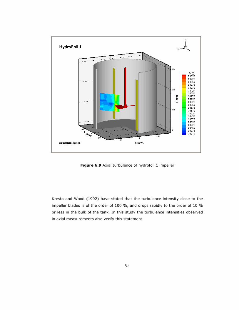
95
Figure 6.9 Axial turbulence of hydrofoil 1 impeller
Kresta and Wood (1992) have stated that the turbulence intensity close to the
impeller blades is of the order of 100 %, and drops rapidly to the order of 10 %
or less in the bulk of the tank. In this study the turbulence intensities observed
in axial measurements also verify this statement.

96
Radial Measurements
Hydrofoil 1 is an axial flow producing impeller consequently it was not expected
to observe any radial flow in the mixing tank. Presence of a large green region,
i.e. low radial component in Figure 6.10, indicates that the flow was mainly in
the axial direction. Radial flow is observed only in the near impeller region and in
between the tank wall and the mixer shaft. The hydrofoil 1 impeller sucks the
fluid and pumps it downwards, during this pumping the fluid inbetween the
mixer shaft and the tank wall is also sucked radially to the near-impeller region.
This is the reason of the partly formed radial flow in the mixing tank. The radial
flow formed between the tank wall and the impeller has a velocity about 0.02 x
tipU , i.e., 40 cm/s, at a height of about D3/1 from the tank bottom mostly close
to the tank wall.
Figure 6.10 Radial dimensionless velocities of hydrofoil 1 impeller
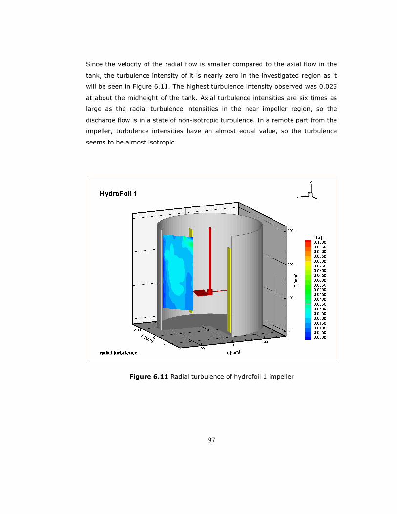
97
Since the velocity of the radial flow is smaller compared to the axial flow in the
tank, the turbulence intensity of it is nearly zero in the investigated region as it
will be seen in Figure 6.11. The highest turbulence intensity observed was 0.025
at about the midheight of the tank. Axial turbulence intensities are six times as
large as the radial turbulence intensities in the near impeller region, so the
discharge flow is in a state of non-isotropic turbulence. In a remote part from the
impeller, turbulence intensities have an almost equal value, so the turbulence
seems to be almost isotropic.
Figure 6.11 Radial turbulence of hydrofoil 1 impeller

98
6.1.3.2. Results of Hydrofoil 2 Impeller
Axial Measurements
The hydrofoil 2 impeller is also an axial flow impeller, the flow field of which is
similar to that of hydrofoil 1’s, however the flow produced by it but is not as
strong as that of hydrofoil 1 impeller’s as can also be understood from mixing
time experiment results given in Part 6.1.1. When the UDV results of hydrofoil 1
and 2 impellers are compared, the similarity in the generated flow will also be
observed as well as the lower velocities occurred in the hydrofoil 2 case. Highest
velocities are observed in the vicinity of the impeller as in the case of hydrofoil 1
impeller. In the impeller region, where the fluid is sucked and pumped axially
downwards, higher velocities are observed; at the red coloured small region in
the vicinity of the impeller velocities reach up to 0.110 x tipU , i.e., 22 cm/s. The
mixing time results also demonstrate the higher efficiency of hydrofoil 1 impeller
compared to hydrofoil 2.

99
Figure 6.12 Axial dimensionless velocities of hydrofoil 2 impeller
The turbulence intensity for axial measurements of hydrofoil 2 impeller is given
in Figure 6.13. Near the impeller region where the fluid is sucked by the
impeller, higher turbulence intensity was observed; in the axial direction of near
impeller region turbulent intensities of about 0.08 were observed while in the
remaining part of the tank they were close to zero.
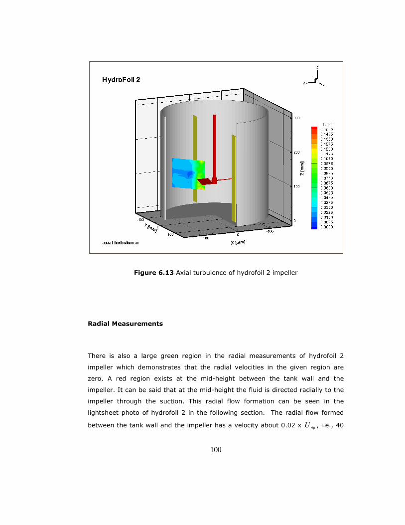
100
Figure 6.13 Axial turbulence of hydrofoil 2 impeller
Radial Measurements
There is also a large green region in the radial measurements of hydrofoil 2
impeller which demonstrates that the radial velocities in the given region are
zero. A red region exists at the mid-height between the tank wall and the
impeller. It can be said that at the mid-height the fluid is directed radially to the
impeller through the suction. This radial flow formation can be seen in the
lightsheet photo of hydrofoil 2 in the following section. The radial flow formed
between the tank wall and the impeller has a velocity about 0.02 x tipU , i.e., 40

101
cm/s, at a height of about D3/1 from the tank bottom in the middle of the mixer
shaft and the tank wall.
Figure 6.14 Radial dimensionless velocities of hydrofoil 2 impeller
The turbulence intensity for radial measurements of hydrofoil 2 impeller is given
in Figure 6.15. Radial turbulence intensities obtained are nearly zero in the
investigated region. Highest turbulence intensities are observed slightly above
the mid-height of the tank with a value of 0.02. Axial turbulence intensities are
four times as large as the radial turbulence intensities at the impeller height, so
the discharge flow is in a state of non-isotropic turbulence. In a remote part from
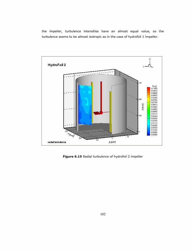
102
the impeller, turbulence intensities have an almost equal value, so the
turbulence seems to be almost isotropic as in the case of hydrofoil 1 impeller.
Figure 6.15 Radial turbulence of hydrofoil 2 impeller

103
6.1.3.4. Results of Combination 1 (submergence of the top hydrofoil
impeller = d)
Axial Measurements
The so called mixer “combination 1” (submergence of the top hydrofoil impeller
= ( d ) and the off-bottom clearance of hyperboloid mixer = ( 10/d )) was also
examined by the UDV method. The results are given in Figure 6.16. The probe
was placed at two positions, 14 cm and 24 cm from the tank bottom, since the
probe could be placed at only these two positions because of the position of the
upper mixer. In between heights 5 cm and 14 cms, a partly red region was
displayed near the mixer shaft where the fluid is pumped axially downwards
along the hyperboloid mixer body. In this region higher axial velocities are
observed at higher measuring points from the tank bottom because of the effect
of the upper hydrofoil 1 impeller. At the highest point maximum velocities reach
up to 0.125 x tipU , i.e., 25 cm/s. As it is approached from the mixer shaft to the
tank wall, first the value of the axially downwards velocities decrease gradually,
and as it is approached to the tank wall the direction of the axially downwards
velocities change; they go axially upwards and increase gradually, which is
displayed as dark blue in Figure 6.16. The maximum value of the axial velocities
that go up along the tank wall are 0.025 x tipU , i.e., 5 cm/s, which is smaller
compared to the axially downwards velocities near the mixer shaft. At the upper
measuring location; between 24 cm and 15 cms from the tank bottom and in
between the upper impeller tip and the tank wall, the value of the axially
downwards velocities are smaller. The value of the axially upwards velocities
near the tank wall are same as the measurements at 9 cm – 14 cms from the
tank bottom.

104
Figure 6.16 Axial dimensionless velocities of hydrofoil 1 and hyperboloid
combination (d)
Axial turbulence of combination 1 is given in Figure 6.17. In the investigated
regions the turbulence intensities are quite close to zero. In the lower measuring
region near the mixer shaft where the highest axial velocities are observed, the
turbulence intensities are about 0.0975 and the highest turbulence intensity
observed was 0.1125.
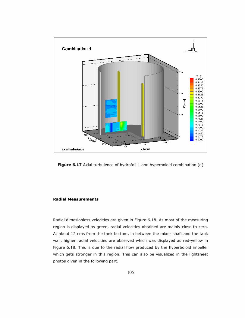
105
Figure 6.17 Axial turbulence of hydrofoil 1 and hyperboloid combination (d)
Radial Measurements
Radial dimesionless velocities are given in Figure 6.18. As most of the measuring
region is displayed as green, radial velocities obtained are mainly close to zero.
At about 12 cms from the tank bottom, in between the mixer shaft and the tank
wall, higher radial velocities are observed which was displayed as red-yellow in
Figure 6.18. This is due to the radial flow produced by the hyperboloid impeller
which gets stronger in this region. This can also be visualized in the lightsheet
photos given in the following part.

106
Figure 6.18 Radial dimensionless velocities of hydrofoil 1 and hyperboloid
combination (d)
Near the tank wall the turbulence intensities are zero. Their values get increased
towards the impeller region. Their distributions are similar to the time mean
velocity distribution in Figure 6.18. Highest turbulence intensity observed is 0.03
near the upper impeller region at a height of D3/2 from the tank bottom. The
S/N ratio was quite low in radial measurements due to the refraction of
ultrasonic beam in the cylindirical tank wall, so insufficient results were obtained
for radial measurements.
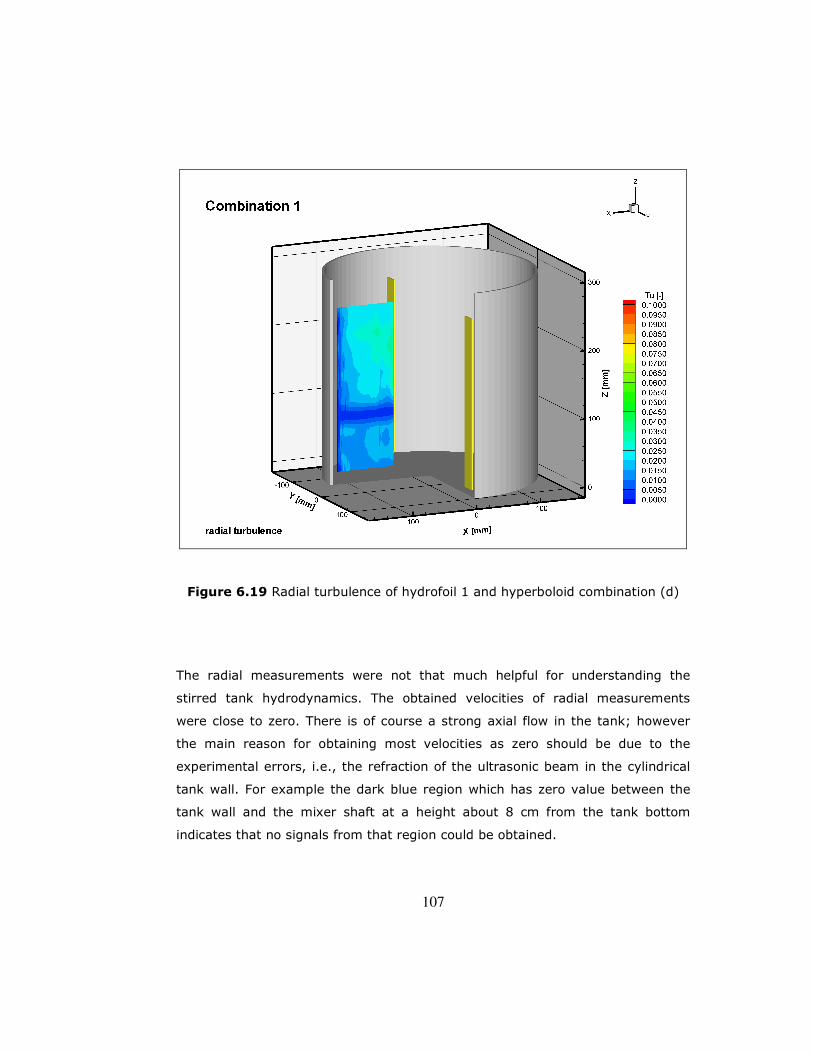
107
Figure 6.19 Radial turbulence of hydrofoil 1 and hyperboloid combination (d)
The radial measurements were not that much helpful for understanding the
stirred tank hydrodynamics. The obtained velocities of radial measurements
were close to zero. There is of course a strong axial flow in the tank; however
the main reason for obtaining most velocities as zero should be due to the
experimental errors, i.e., the refraction of the ultrasonic beam in the cylindrical
tank wall. For example the dark blue region which has zero value between the
tank wall and the mixer shaft at a height about 8 cm from the tank bottom
indicates that no signals from that region could be obtained.

108
6.1.3.5. Results of Combination 2 (submergence of the top hydrofoil impeller = 1.5d)
The so called mixer “combination 2” (submergence of the top hydrofoil impeller
= d5.1 and the off-bottom clearance of hyperboloid mixer = 10/d ) was also
examined by the UDV method. The results can be seen in Figure 6.20. The probe
was placed at two positions, 14 cm and 24 cm from the tank bottom. In between
heights 5 cm and 14 cms, a partly red region was displayed near the mixer shaft
where the fluid is pumped axially downwards along the hyperboloid mixer body,
as in the case of mixer combination 1. In this region higher axial velocities are
observed at higher measuring points from the tank bottom because of the effect
of the upper hydrofoil 1 impeller. Since the position of the hydrofoil 1 impeller in
mixer combination 2 is closer to the measuring location compared to its position
in mixer combination 1, the red region showing the downward axial velocities is
intenser. Maximum velocity observed was 0.125 x tipU , i.e., 25 cm/s. As it is
approached from the mixer shaft to the tank wall, first the value of the axially
downwards velocities decrease gradually, and as it is approached to the tank
wall the direction of the axially downwards velocities change; they go axially
upwards and increase gradually, which is displayed as dark blue in Figure 6.20.
The change to axially downwards velocities from axially upwards velocities, from
the mixer towards the tank wall) occurs more gradual in mixer combination 2
compared to mixer combination 1. The value of the axially upwards velocities in
the vicinity of the tank wall at 9 cm – 14 cms from the tank bottom are the same
as the upwards velocities in the vicinity of the tank wall at 24 cm – 15 cms from
the tank bottom. However the highest axially downward velocities at 24 cm – 15
cms in the vicinity of the tank wall extends radially towards the impeller for a
larger region compared to velocities at 9 cm – 14 cms from the tank bottom, the
change is more gradual in the lower part of the tank.
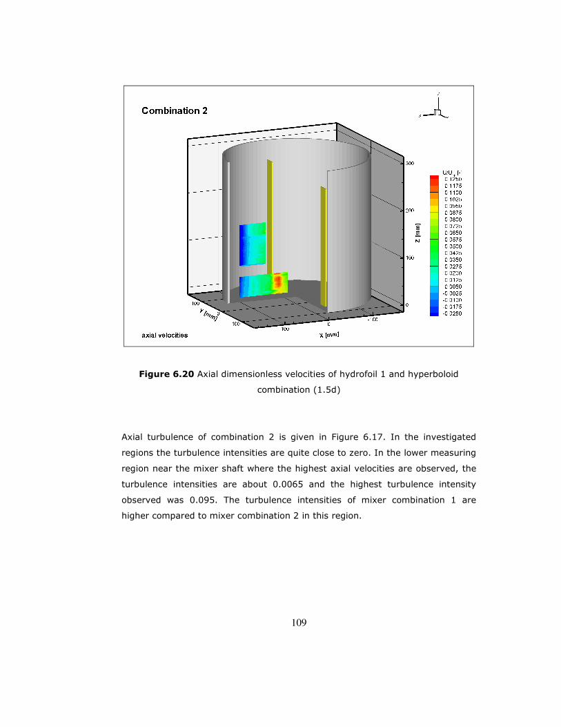
109
Figure 6.20 Axial dimensionless velocities of hydrofoil 1 and hyperboloid
combination (1.5d)
Axial turbulence of combination 2 is given in Figure 6.17. In the investigated
regions the turbulence intensities are quite close to zero. In the lower measuring
region near the mixer shaft where the highest axial velocities are observed, the
turbulence intensities are about 0.0065 and the highest turbulence intensity
observed was 0.095. The turbulence intensities of mixer combination 1 are
higher compared to mixer combination 2 in this region.

110
Figure 6.21 Axial turbulence of hydrofoil 1 and hyperboloid combination 2
(1.5d)
Radial Measurements
Radial dimesionless velocities are given in Figure 6.22. As most of the measured
region is displayed as green, radial velocities obtained are mainly close to zero.
At the midheight of the tank, in between the mixer shaft and the tank wall,
higher radial velocities are observed which was displayed as red in Figure 6.22. A
radial flow is formed in this region at the upper mixer height, where the part of
the fluid (leaving the hyperboloid impeller, going radially over the tank bottom,
going up the tank wall) returning back to the hyperboloid impeller body, is
sucked by the hydrofoil 1 impeller together with the fluid in the upper-half part

111
of the tank. This can also be visualized in the lightsheet photos given in the
following part.
Figure 6.22 Radial dimensionless velocities of hydrofoil 1 and hyperboloid
combination (1.5d)
Near the tank wall the turbulence intensities are zero. Their values get increased
as it is approached to the impeller region. Their distributions are similar to the
time mean velocity distribution in Figure 6.21. Highest turbulence intensity
observed is 0.035 near the impeller region at the midheight of the tank. As it has
been stated, the S/N ratio was quite low in radial measurements due to the
refraction of ultrasonic beam in the cylindirical tank wall. It is recommended to
the place the probe to a hole which has been made on the tank wall up to certain

112
deepness or to place the vessel in a square Plexiglas tank filled with water, which
was used by Armenante et al. (1997), in order to minimize the refractive effects
at the curved surface of the mixing vessel.
Figure 6.23 Radial turbulence of hydrofoil 1 and hyperboloid combination (1.5d)
113
6.1.4. Flow Visualization (Lightsheet) Experiments
Lightsheet experiments were performed for hydrofoil 1, hydrofoil 2, hyperboloid
impellers and the two impeller combinations. The extracted pictures of the video
records are given below. The pictures allow one to observe general flow
characteristics of the impellers qualitatively. It should be noted that quantitative
analysis of these results are not possible as opposed to the UDV experiments at
which velocities and turbulence intensities were determined.
Armenante et al. (1997) have worked with a downward pumping, six-blade, 45º
pitched-blade turbine with a dD / ratio of 3 in an unbaffled tank at two
Reynolds numbers; 71000 and 111000. They have found that the dimensionless
velocity and turbulent kinetic energy profiles were nearly identical at two
different agitation speeds indicating that the impeller speed plays a minor role in
the direction and magnitude of the dimensionless velocities and turbulent kinetic
energies at any point (including the region near the impeller). In this study the
UDV and lightsheet experiments were performed in the turbulent regime at
different Reynolds numbers, as stated in the work of Armenante et al. (1997)
the flow field at different Reynolds number do not differ from each other.
The axial flow produced by the hydrofoil 1 impeller can be seen in Figure 6.24.
The fluid is sucked by the impeller and pumped down axially, goes along the
tank bottom, goes up the tank wall and returns to the impeller again. The upper
part, above the impeller region, is also in motion since the flow going up the
tank wall, returning back to impeller also carries the unmoving fluid in the upper
part of the tank to the impeller region so that a movement occurs in all over the
tank and no dead zones exist. This can be visualized in the lightsheet movie
given in Appendix F. This complete movement in the overall tank and of course
the power consumption characteristics of the hydrofoil 1 impeller makes it the
most efficient impeller in macromixing time experiments among other
investigated impeller configurations.

114
Figure 6.24 Lightsheet photo of the hydrofoil 1 impeller
Hydrofoil 2 impeller provides a similar flow field to that of hydrofoil 1 as can be
seen in Figure 6.25. A complete movement in the whole tank without any dead
zones was observed. The complete movement in the overall tank is the
advantage of the hydrofoil 2 impeller however when its power consumption and
macromixing characteristics are considered hydrofoil 1 impeller is more efficient
compared to hydrofoil 2 impeller.

115
Figure 6.25 Lightsheet photo of the hydrofoil 2 impeller
Hyperboloid impeller provides a radial flow originated from the mixer-body over
the tank bottom, going up the wall and returning to the centre of the mixed cell.
But this circulation pattern is mainly confined to the regions closer to the tank
bottom. This can be seen in Figure 6.26. There is a movement in all over the
tank however the movements in the fluid higher than a D/2 clearence is slower
compared to the lower part of the tank, which was not the case in hydrofoil 1
and 2 impellers. This is the main reason why the hyperboloid impeller had the
highest mixing time at equal power consumption in macromixing measurements,
especially when the injection point of the tracer solution is considered. These
types of mixers are especially used for the mixing of suspensions, i.e. for
preventing the sedimentation of the particles in suspensions.
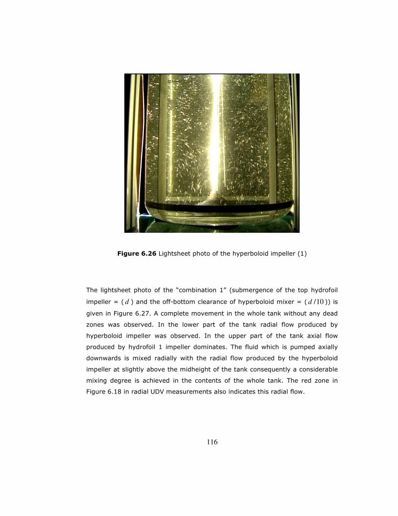
116
Figure 6.26 Lightsheet photo of the hyperboloid impeller (1)
The lightsheet photo of the “combination 1” (submergence of the top hydrofoil
impeller = ( d ) and the off-bottom clearance of hyperboloid mixer = ( 10/d )) is
given in Figure 6.27. A complete movement in the whole tank without any dead
zones was observed. In the lower part of the tank radial flow produced by
hyperboloid impeller was observed. In the upper part of the tank axial flow
produced by hydrofoil 1 impeller dominates. The fluid which is pumped axially
downwards is mixed radially with the radial flow produced by the hyperboloid
impeller at slightly above the midheight of the tank consequently a considerable
mixing degree is achieved in the contents of the whole tank. The red zone in
Figure 6.18 in radial UDV measurements also indicates this radial flow.

117
Figure 6.27 Lightsheet photo of mixer combination (d)
The lightsheet photo of the “combination 2” (submergence of the top hydrofoil
impeller = ( d5.1 ) and the off-bottom clearance of hyperboloid mixer = ( 10/d ))
is given in Figure 6.28. A complete movement in the whole tank without any
dead zones was also observed. Hydrofoil 1 impeller which is located at the
midheight of the tank produces an axial flow which also disturbs the radial flow
produced by hyperboloid impeller. The radial flow formed by the hyperboloid
impeller reaches the tank wall and formes a circular flow there and than this flow
is disturbed by the axial pumping of the hydrofoil 1 impeller. In lower half part of
the tank a considerable mixing degree is achieved. The fluid in the upper half
part of the tank is sucked by the hydrofoil impeller and a radial flow occurs
during this pumping at the midheight of the tank. The mixing in the upper part
of the tank is slower compared to that of the “combination1”. The red zone in
Figure 6.18 in radial UDV measurements also indicates this radial flow.
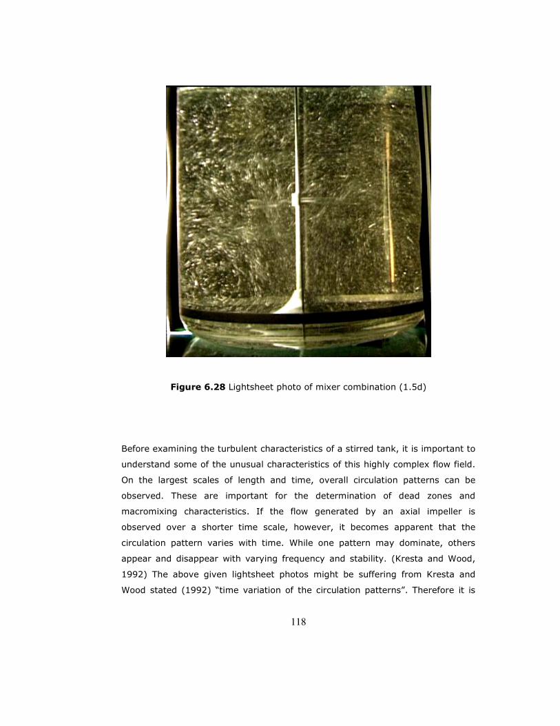
118
Figure 6.28 Lightsheet photo of mixer combination (1.5d)
Before examining the turbulent characteristics of a stirred tank, it is important to
understand some of the unusual characteristics of this highly complex flow field.
On the largest scales of length and time, overall circulation patterns can be
observed. These are important for the determination of dead zones and
macromixing characteristics. If the flow generated by an axial impeller is
observed over a shorter time scale, however, it becomes apparent that the
circulation pattern varies with time. While one pattern may dominate, others
appear and disappear with varying frequency and stability. (Kresta and Wood,
1992) The above given lightsheet photos might be suffering from Kresta and
Wood stated (1992) “time variation of the circulation patterns”. Therefore it is

119
recommended that the lightsheet movie CD given in Appendix G is seen, so that
the appearing and disappearing patterns with change of time are best visualized.
6.2. Square Tank Experiments
6.2.1. Macromixing Measurements in the Square Tank
Macromixing time measurements were carried out at four different impeller
speeds that were in the turbulent regime. Three impeller types were employed in
the 900 mm square tank measurements. These are Generation 5 low and high
rib impellers and Generation 6 hyperboloid impeller photos of which are given in
Figure 5.10, 5.11 and 5.12. The ribs of Generation 5 high rib impeller are higher
than that of Generation 5 low rib’s. Generation 6 had the highest transport ribs
extending from mixer tip to mixer hub and additional holes on the mixer hub. It
has also a profiled bottom which also affects its efficiency. In Figure 6.29
variation of mixing time with rotational speed is shown. The mixing time values
of square tank experiments are generally about 10 times higher the cylindrical
tank mixing time values experiments. The water volume in the square tank is
about 18 times the water volume in the cylindrical tank. Generation 5 low rib
impeller is used both in the cylindrical tank and square tank experiments. The
improvements in the mixer geometry of the hyperboloid impellers resulted in
considerable differences in the mixing times.
For the measured mixing times the dimensionless mixing time θn was obtained
and in Figure 6.30 the θn versus Reynolds number graph is shown. The highest
mixing time value obtained was Generation 5 low rib hyperboloid’s impeller,
while the smallest one was Generation 6’s.
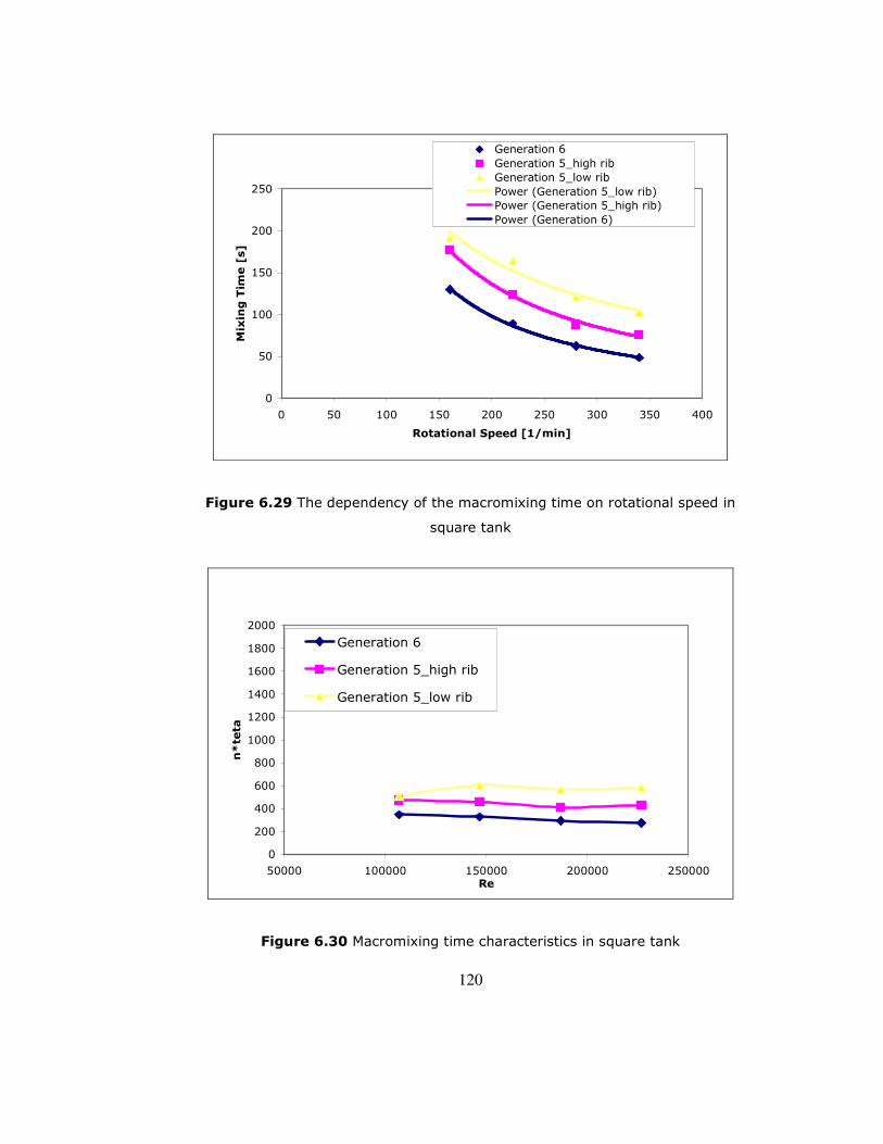
120
0
50
100
150
200
250
0 50 100 150 200 250 300 350 400
Rotational Speed [1/min]
Mixing Time [s]
Generation 6Generation 5_high ribGeneration 5_low ribPower (Generation 5_low rib)Power (Generation 5_high rib)Power (Generation 6)
Figure 6.29 The dependency of the macromixing time on rotational speed in
square tank
0
200
400
600
800
1000
1200
1400
1600
1800
2000
50000 100000 150000 200000 250000Re
n*teta
Generation 6
Generation 5_high rib
Generation 5_low rib
Figure 6.30 Macromixing time characteristics in square tank
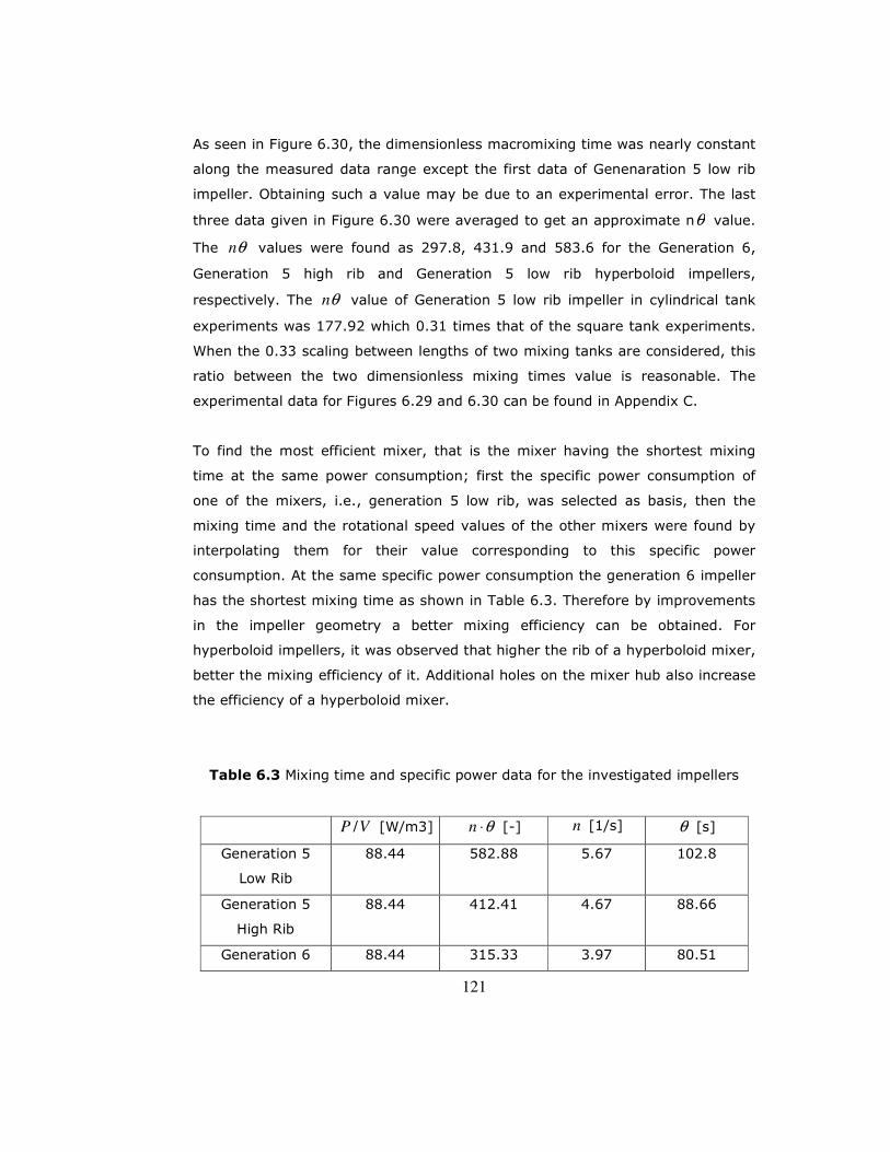
121
As seen in Figure 6.30, the dimensionless macromixing time was nearly constant
along the measured data range except the first data of Genenaration 5 low rib
impeller. Obtaining such a value may be due to an experimental error. The last
three data given in Figure 6.30 were averaged to get an approximate nθ value.
The θn values were found as 297.8, 431.9 and 583.6 for the Generation 6,
Generation 5 high rib and Generation 5 low rib hyperboloid impellers,
respectively. The θn value of Generation 5 low rib impeller in cylindrical tank
experiments was 177.92 which 0.31 times that of the square tank experiments.
When the 0.33 scaling between lengths of two mixing tanks are considered, this
ratio between the two dimensionless mixing times value is reasonable. The
experimental data for Figures 6.29 and 6.30 can be found in Appendix C.
To find the most efficient mixer, that is the mixer having the shortest mixing
time at the same power consumption; first the specific power consumption of
one of the mixers, i.e., generation 5 low rib, was selected as basis, then the
mixing time and the rotational speed values of the other mixers were found by
interpolating them for their value corresponding to this specific power
consumption. At the same specific power consumption the generation 6 impeller
has the shortest mixing time as shown in Table 6.3. Therefore by improvements
in the impeller geometry a better mixing efficiency can be obtained. For
hyperboloid impellers, it was observed that higher the rib of a hyperboloid mixer,
better the mixing efficiency of it. Additional holes on the mixer hub also increase
the efficiency of a hyperboloid mixer.
Table 6.3 Mixing time and specific power data for the investigated impellers
VP / [W/m3] θ⋅n [-] n [1/s] θ [s]
Generation 5
Low Rib
88.44 582.88 5.67 102.8
Generation 5
High Rib
88.44 412.41 4.67 88.66
Generation 6 88.44 315.33 3.97 80.51
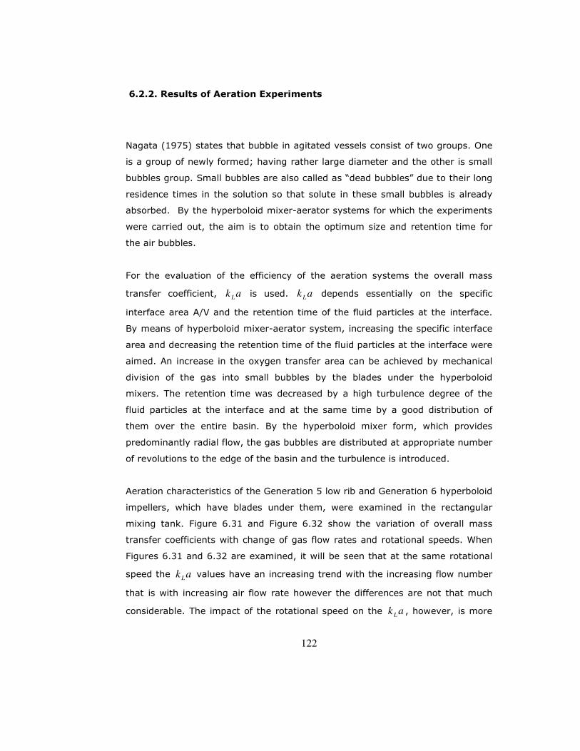
122
6.2.2. Results of Aeration Experiments
Nagata (1975) states that bubble in agitated vessels consist of two groups. One
is a group of newly formed; having rather large diameter and the other is small
bubbles group. Small bubbles are also called as “dead bubbles” due to their long
residence times in the solution so that solute in these small bubbles is already
absorbed. By the hyperboloid mixer-aerator systems for which the experiments
were carried out, the aim is to obtain the optimum size and retention time for
the air bubbles.
For the evaluation of the efficiency of the aeration systems the overall mass
transfer coefficient, akL is used. akL depends essentially on the specific
interface area A/V and the retention time of the fluid particles at the interface.
By means of hyperboloid mixer-aerator system, increasing the specific interface
area and decreasing the retention time of the fluid particles at the interface were
aimed. An increase in the oxygen transfer area can be achieved by mechanical
division of the gas into small bubbles by the blades under the hyperboloid
mixers. The retention time was decreased by a high turbulence degree of the
fluid particles at the interface and at the same time by a good distribution of
them over the entire basin. By the hyperboloid mixer form, which provides
predominantly radial flow, the gas bubbles are distributed at appropriate number
of revolutions to the edge of the basin and the turbulence is introduced.
Aeration characteristics of the Generation 5 low rib and Generation 6 hyperboloid
impellers, which have blades under them, were examined in the rectangular
mixing tank. Figure 6.31 and Figure 6.32 show the variation of overall mass
transfer coefficients with change of gas flow rates and rotational speeds. When
Figures 6.31 and 6.32 are examined, it will be seen that at the same rotational
speed the akL values have an increasing trend with the increasing flow number
that is with increasing air flow rate however the differences are not that much
considerable. The impact of the rotational speed on the akL , however, is more
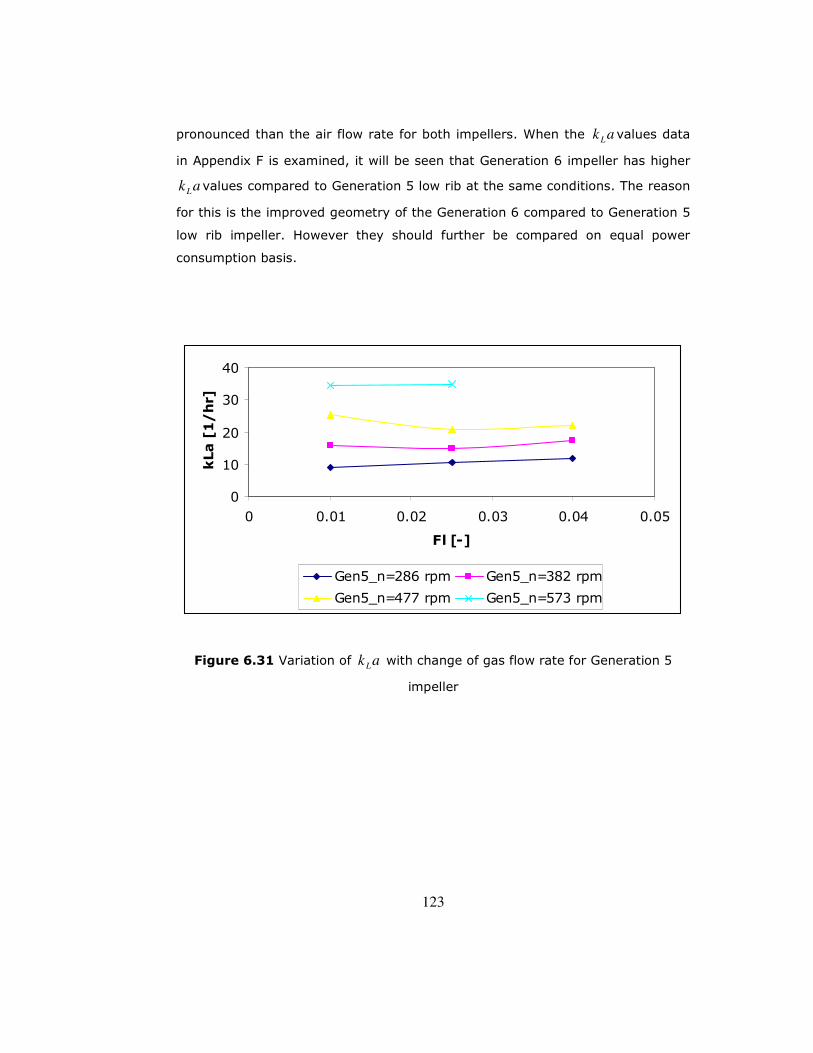
123
pronounced than the air flow rate for both impellers. When the akL values data
in Appendix F is examined, it will be seen that Generation 6 impeller has higher
akL values compared to Generation 5 low rib at the same conditions. The reason
for this is the improved geometry of the Generation 6 compared to Generation 5
low rib impeller. However they should further be compared on equal power
consumption basis.
0
10
20
30
40
0 0.01 0.02 0.03 0.04 0.05
Fl [-]
kLa [1/hr]
Gen5_n=286 rpm Gen5_n=382 rpm
Gen5_n=477 rpm Gen5_n=573 rpm
Figure 6.31 Variation of akL with change of gas flow rate for Generation 5
impeller

124
0.00
10.00
20.00
30.00
40.00
50.00
0 0.01 0.02 0.03 0.04 0.05
Fl [-]
kLa [1/hr]
Gen6_n=286 rpm Gen6_n=382 rpm
Gen6_n=477 rpm Gen6_n=573 rpm
Figure 6.32 Variation of akL with change of gas flow rate for Generation 6
impeller
At different rotational speeds and air flow rates, the specific oxygen capacity of
water in the tank was investigated. The results are shown in Figures 6.33 and
6.34. Fl is the dimensionless flow number,3* dn
QFl A= , where AQ is the air flow
rate [m3/s] with an oxygen concentration of 0.299 kg/m3, n is the rotational
speed [s-1] and d is the diameter of the mixer [m], OA [%] is the oxygen
utilization efficiency which is equal to )99.2*Q(
*100
A
OCOA = . Here OC is the oxygen
concentration in the mixing tank. By increasing the rotational speed the oxygen
transfer efficiency also increases at Fl =0.01. As the flow number increases the
differences in the efficiencies at different rotational speeds decrease for both
impellers. At Fl =0.04 both impellers exhibit nearly the same performance. It
can be said that when the air flow rate is small the air transferred to the system
is dominated by the mixing efficiency of impeller. When the air flow rate is large,

125
the effect of the impellers mixing efficiency is minimized. To achieve an optimum
working condition at a treatment plant, the cost of the power consumption of the
pressurized air should be considered together with power consumption of the
mixer. When Figures 6.33 and 6.34 are compared, it will be seen that Generation
6 impeller exhibit higher OA values at the same conditions. This behaviour can
be seen in Figures 6.35, 6.36 and 6.37 in a more detailed form. In these figures
the transferred oxygen amounts are also compared at different rotational speeds
for the same flow numbers, and in each case Generation 6 impeller exhibited
higher OC values.
0
5
10
15
20
0 0.01 0.02 0.03 0.04 0.05
Fl [-]
OA [%]
n=286 [1/min] n=382 [1/min]
n=477 [1/min] n=573 [1/min]
Figure 6.33 Variation of OA [%] with Fl [-] at different rotational speeds for
Generation 5
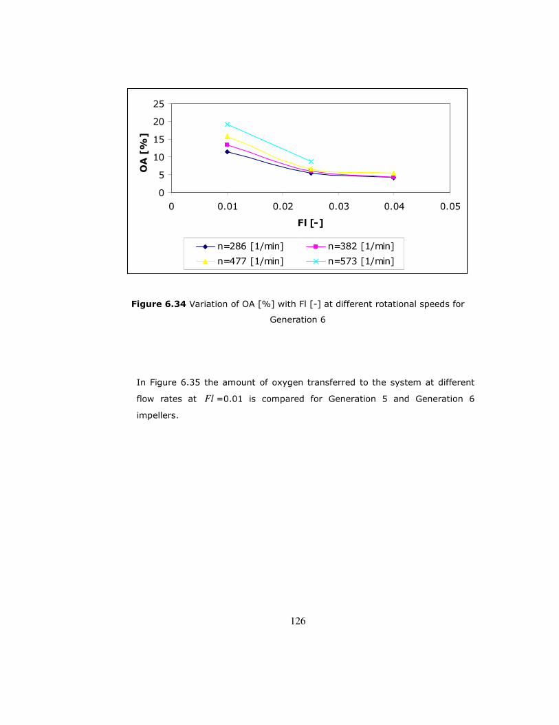
126
0
5
10
15
20
25
0 0.01 0.02 0.03 0.04 0.05
Fl [-]
OA [%]
n=286 [1/min] n=382 [1/min]
n=477 [1/min] n=573 [1/min]
Figure 6.34 Variation of OA [%] with Fl [-] at different rotational speeds for
Generation 6
In Figure 6.35 the amount of oxygen transferred to the system at different
flow rates at Fl =0.01 is compared for Generation 5 and Generation 6
impellers.
127
020406080
100120140160180
0 200 400 600 800
Rotational Speed [1/min]
OC [kg/h]
Gen5 _Fl=0.01 Gen6_Fl=0.01
Figure 6.35 Amount of oxygen transferred to the system at Fl=0.01 for
Generation 5 and Generation 6
Generation 6 impeller exhibited a better performance about 20% than
Generation 5 impeller. This is due to improved design of Generation 6 impeller.
Higher transport ribs extending from mixer tip to mixer hub and additional holes
on the mixer hub provide Generation 6 impeller a better performance. As can be
seen in Figures 6.36 and 6.37, the Generation 6 provides a better performance
compared to Generation 6 also at Fl =0.025 and Fl =0.04. These results should
also be compared on equal power consumption basis in order to decide about the
efficiencies of the mixer aerator systems.

128
020406080
100120140160180200
0 200 400 600 800
Rotational Speed [1/min]
OC [kg/h]
Gen5_Fl=0.025 Gen6_Fl=0.025
Figure 6.36 Amount of oxygen transferred to the system at Fl=0.025 for
Generation 5 and Generation 6
020406080
100120140160180200
0 200 400 600 800
Rotational Speed [1/min]
OC [kg/h]
Gen5_Fl=0.04 Gen6_Fl=0.04
Figure 6.37 Amount of oxygen transferred to the system at Fl=0.04 for
Generation 5 and Generation 6
129
Nagata (1975) have stated the major factors in order to apply shear forces
effectively on to the bubbles as follows:
• Gas inlet pipe should be set close to the impeller blades
• Gas should be blown from many holes bored in a ring sparger than from a
single nozzle.
• The loop diameter of discharge hole arrangement is chosen to be 80% of
the impeller diameter
As a remark, it should be added that the investigated hyperboloid mixer-aerator
configurations conforms to the factors stated above.
130
CHAPTER VII
CONCLUSIONS
Macromixing and power consumption measurements were performed in the 300
mm diameter cylindrical tank and experimental data have been analyzed on the
basis of equal power consumption. From two new design hydrofoil impellers, the
so called hydrofoil 1 impeller had a shorter mixing time than the hydrofoil 2
impeller at equal power consumption; this is mainly due to smaller blade
thickness and hub length of the hydrofoil 1 impeller as well as its improved blade
angle. These two impellers have considerably low Newton numbers compared to
that of the standard impellers’. Their mixing times were also comparable to that
of the standard impellers’. For all the impellers and impeller combinations
investigated, the θn value, the product of mixing time and impeller rotational
speed, was constant. It changed depending on the impeller type. The flow fields
produced by the impellers where also investigated quantitatively by UDV. In
axial UDV measurements the turbulence intensity close to the impeller blades is
about 10 times of the bulk of the tank. Unsatisfactory results were obtained for
radial measurements due to refractive effects at the curved surface of the mixing
vessel. Flow visualization experiments performed in the cylindrical tank also
provided qualitative information about the flow field. From both UDV and
lightsheet observations, it can be concluded that both hydrofoil impellers were
found to have a strong pumping capacity, providing a top to bottom circulation in
the stirred tank. This study indicates that impeller design greatly affects the
mixing time; minor dimensions such as impeller hub, blade width and thickness
play an important role in the mixing efficiency. In this respect the new design
hydrofoil type impellers can also be improved with changes in their minor
parameters and a higher discharge flow may be obtained at lower power
consumption.

131
Macromixing measurements were also performed in a 900x900 mm square tank
for three different generations of hyperboloid impellers. These were Generation 5
low rib, Generation 5 high rib and Generation 6 impellers. Generation 5 low rib
and Generation 5 high rib impellers were of the same geometry, the only
difference was that Generation 5-high rib had a higher rib height. Generation 6
has a similar geometry to Generation 5 high rib however its transport ribs
reaches to the upper part of the impeller, the ribs get higher as they go up and
at the upper part there are holes in between them. It has also a corrugated
bottom. For all the three types of hyperboloid impellers, θn , the product of
mixing time and impeller rotational speed, was constant. These three different
designs of hyperboloid impellers were compared for their mixing time on the
basis of equal power consumption. The mixing times at equal power
consumption were found as 6Genθ < highribGen5θ < lowribGen5θ . From this result, it can
again be concluded that improving the minor dimensions of an impeller can lead
to an increase in its mixing efficiency.
Aeration characteristics of Generation 5 low rib and Generation 6 impellers,
which have blades under them for aeration purposes, were investigated. When
the air flow rate sent to the mixer-aerator system is small, the amount of
dispersed oxygen in the system is dominated by the mixing efficiency of
impeller. When the air flow rate is large, the affect of the impellers mixing
efficiency is minimized. To achieve an optimum working condition at a treatment
plant, the cost of the power consumption of the pressurized air should be
considered together with power consumption of the mixer. Generation 6 impeller
exhibit higher oxygen transfer efficiencies at the same rotational speeds and air
flow rates compared to Generation 5 low rib impeller. This is due to the
improved design of the Generation 6 impeller. However, these mixer-aerators
should be compared on the basis of equal power consumption so that the mixer
with the higher efficiency can be done.

132
CHAPTER VIII
RECOMMENDATIONS
Different techniques can be used for the determination of the mixing time to
have mixing grade lower than 10%. Multiple probes can be helpful for the
determination of the slow mixing zones.
Further mixing efficiency tests should be carried out with hydrofoil type of
impellers by making changes in their minor dimensions. Lowering the Dd / ratio
may also provide a better mixing efficiency. The use of empirical equations of
Ruszkowski is still helpful for the estimation of the mixing times of the hydrofoil
impellers.
UDV measurements are not helpful when the probe is directly mounted on the
cylindrical tank with the ultrasonic gel as the coupling medium. It is
recommended that the probe be placed on a hole made in the tank wall up to a
certain depth so that the refractions of the ultrasonic beams can be kept at
minimum. The cylindrical vessel can be also placed in a square Plexiglas tank
filled with water and the probe can be placed on the outer side of the square
tank.
In the lightsheet experiments it is recommended to change the water in the tank
before each recording since the aluminum particles got dissolved in water and
disabled the visualization of the flow field.

133
Power consumption tests of the hyperboloid mixer-aerator systems should be
performed so that a comparison of the efficiencies on the basis of equal power
consumption can further be done.

134
REFERENCES
1. Alves, S.S., Vasconcelos, J.M.T., Orvalho, S.P., “Mass transfer to clean bubbles at low turbulent energy dissipation” Chemical Engineering Science, article in press. (2005)
2. Armenante, M. P., Luo, C., Chou, C., Fort, I., Medek, J., “Velocity profiles
in a closed vessel: comparison between experimental LDV data and numerical CFD predictions” Chemical Engineering Science, Vol.52 (20), pp. 3483-3492. (1997)
3. ATV-Arbeitsblatt M 209, Regelwerk Abwasser-Abfall, Messung der
Sauerstoffzufuhr von Belüftungseinrichtungen in Belebungsanlagen, in Reinwasser und in belebtem Schlamm, Abwassertechnische Reinigung e.V. (1996)
4. Batchelor, G. K., The Theory of Homogenous Turbulence, Univ. Press.,
Cambridge. (1953)
5. Bishof, F., “Untersuchung der Blasenbildung und des Stoffaustausches unter dem Einfluss oberflächenaktiver Substanzen und gelöster Gase”, Dissertation, Universität Erlangen-Nürnberg. (1994)
6. Bouillard, J., Alban., B., Jacques, P., Xuereb, C., “Liquid velocity flow
measurements in stirred tanks by ultra-sound Doppler Velocimetry”, Chemical Engineering Science, Vol.56, pp. 747-754. (2001)
7. Brito, D., Nataf., H., Cardin, P., Aubert, J., Masson, J., “Ultrasonic Doppler
velocimetry in liquid gallium”, Experiments in Fluids, Vol.31, No.6, pp 653-663. (2001)
8. Brodkey, R.S., “Mixing, Theory and Practice”, Academic Press New York-
London. (1966)
9. Calderbank, P.H., Moo-Young, M.B., “The continuous phase heat and mass transfer of dispersions”, Chemical Engineering Science, Vol.16, pp. 39-54. (1961)
10. Corrsin, S., Vol.12, pp. 403, AIChE Journal. (1968)
11. Costes, J., Couderc, J. P., “Study by laser Doppler anemometry of the
turbulent flow induced by a Rushton turbine in a stirred tank: influence of the size of the units (Parts I&II)”, Chemical Engineering Science, Vol.43 (10), pp. 2754-2772. (1988)
135
12. Chisti, Y., Jauregui-Haza, U.J., “Oxygen transfer and mixing in mechanically agitated airlift bioreactors”, Biochemical Engineering Journal, Vol.10, pp 143-153. (2001)
13. Ciofalo, M., Brucato, A., Grisafi, F., Torraca, N., “Turbulent flow in closed and free-surface unbaffled tank stirred by radial impellers”, Chemical Engineering Science, Vol.51 (14), pp. 3557-3573. (1988)
14. Danckwerts, P.V., “Significance of liquid-film coefficients in gas
absorption”, Industrial and Engineering Chemistry 43, pp.1460–1467. (1951)
15. Fentiman, N. J., Hill, N.S., Lee, K.C., Paul G.R., Yianneskis, M.A., “Novel
Profiled Blade Impeller for Homogenization of Miscible Liquids in Stirred Vessels”, Trans. Inst. Chem. Eng., 76A, 835. (1998)
16. Frey, T., Entwicklung verbesserter Auslegungsrichtlininen für
Begasungssysteme und Valideirung in der Praxis, Masters thesis, Universität Erlangen-Nürnberg. (1999)
17. Gao, Z., Niu, G., Shi. L., Smith, J. M., “Mixing in Stirred Tanks with
Multiple Hydrofoil Impellers”, 11th European Conference on Mixing, Bamberg. (2003)
18. Hiby, J. W., “Definition und Messung der Mischgüte in flüssigen
Gemischen”, Chem.-Ing.-Tech., Vol. 51, pp. 704-709. (1979)
19. Hinze, J.O., Turbulence McGraw-Hill. (1959)
20. Higbie, R., “The rate of absorption of a pure gas into a still liquid during a short time of exposure”, Transactions of the American Institute of Chemical Engineers 31, 365–389. (1935)
21. Höfken, M., Bischof, F. und Durst, F., “Untersuchungen von Rühr- und
Mischvorgängen mit Hilfe der Ultraschall-Doppler-Anemometrie”, Erlangen. (1995)
22. Höfken, M. : Moderne experimentelle Methoden für die Untersuchung von
Strömungen in Rührbehältern und für Rührwerksoptimierung, Dissertation, Erlangen. (1994)
23. Höfken, M., Steidl, W., Huber P., “About the Design of Mixing Systems for
Anaerobic and Anoxic Basins for Large Wastewater Treatment Plants”, MIXIN XIX, North American Mixing Forum. (2003)
24. Kawase, Y., Halard, B., Moo-Young, M., “Theoretical prediction of
volumetric mass transfer coefficients in bubble columns for Newtonian and non-Newtonian fluids”, Chemical Engineering Science, Vol. 42, pp. 1609–1617. (1987)

136
25. Khang, S. J., Levenspiel, O., “New Scale-up and Design Method for Stirrer Agitated Batch Mixing Vessels”, Chemical Engineering Science, Vol. 31, pp. 569-577. (1976)
26. Kolmogoroff, A.N., C.R. (Doklady) Acad. Sci. U.S.S.R, Vol.30, pp. 301.
(1941)
27. Kresta, M.S., Wood, P.E., “The flow field produced by a pitched blade turbine: Characterization of the turbulence and estimation of the dissipation rate”, Chemical Engineering Science, Vol. 42 (10), pp. 1761–1774. (1993)
28. Lamont, J.C., Scott, D.S., “An eddy cell model of mass transfer into
surface of a turbulent liquid”, American Institute of Chemical Engineers Journal 16, 513–519. (1970)
29. Levenspiel, O., Chemical Reaction Engineering, John Wiley&Sons: New
York. (1991) 30. Mann, R., Dickin., F.J., Wang, M., Dyakowski, T., Williams, R.B., Edwards,
R.B., Forrest, P. J., Holden, P.J., “Application of Electrical Resistance Tomography to Interrogate Mixing Processes at Plant Scale”, Chemical Engineering Science, Vol. 52, pp 2087-2097. (1997)
31. Motarjemi, M., Jameson, G.J., „Mass Transfer from very small bubbles-
the optimum bubble size for aeration”, Chem. Eng. Sci., Vol. 33, pp 1415-1423. (1978)
32. Mersmann, A., Geisler, R. : Strömungsmechanische Grundlagen des
Rührens, Hochschulkurs Rühr- und Mischtechnik, München. (1994)
33. Met-Flow SA, “UVP Method”, www.met-flow.com, 2005, last access date May 2006.
34. Nagata, S., Mixing – Principles and Applications, Kodansha Ltd., Tokyo.
(1975)
35. Nath, B., Löber, W., Baetz, W., Holzapfel, W., “Laser Light Sheet Imaging of Gas Flow with Laser Diodes”, Vol. 3 (1), pp. 102-199. (1999)
36. Nere, N. K., Patwarhan, A.W. and Joshi, J. B., “Liquid Phase Mixing in
Stirred Vessels: Turbulent Flow Regime”, Ind. Eng. Chem.. Res., Vol. 42, pp. 2661-2698. (2003)
37. Nowak, M., “Wall shear stress measurement in a turbulent pipe flow using
ultrasound Doppler velocimetry”, Experiments in Fluids, Vol. 33, pp. 249-255. (2002)
38. Operational Manual Ultrasonic Velocity Profile Monitor, Ser. No 10202.
(1991)

137
39. Ozaki, Y., Tatsuya, K., Takeda, Y., Hishida, K., Masanobu, M., High Time Resolution Ultrasonic Velocity Profiler, Experimental Thermal and Fluid Science, Vol. 26, pp. 253-258. (2001)
40. Pasveer, A., “Oxygenation of Water with Air Bubbles”, Sewage and Industrial Waste, Vol.27, pp.1130-1146. (1955)
41. Prasher, B.D., Wills, G.B., Mass transfer in an agitated vessel, Industrial and Engineering Chemistry Process Design and Development, Vol. 12, pp. 351 354. (1973)
42. Prochazka, J.; Landau, J., “Homogenization of Miscible Liquids in the Turbulent Region”, Collect. Czech. Chem. Commun., Vol. 26, pp. 2961. (1961)
43. Ranade, V.V., Joshi, J.B., “Flow generated by a disc turbine: Part I. Experimental”, Trans. Instn. Chem. Engng, Vol. 68(A), 19-33. (1990a)
44. R. Rao, K. S. M. S.; Joshi, J.B., “Liquid Phase Mixing in Mechanically Agitated Vessels”, Chem. Eng. Commun., Vol. 74, pp.1. (1988)
45. Rewatkar, V.B., Joshi J.B., Effect of Impeller Design on Liquid Phase Mixing in Mechanically Agitated Reactors, Chem. Eng. Commun., Vol. 91, pp. 322. (1991)
46. Rielly, C.D.; Britter, “R.E. Mixing Times for Passive Tracers in Stirred Tanks”, Proc. 5th Eur. Conf. Mixing, pp. 365. (1985)
47. Ruszkowski, S. A., “Rational Method for Measuring Blending Performance and Comparison of Different Impeller Types”, Proc. Eighth Eur. Conf. Mixing, pp. 283. (1994)
48. Sano, Y., Usui, H., “Interrelations Among Mixing Time, Power. Number
and Discharge Flow Rate Number”, J. Chem. Eng. Japan, Vol. 18, pp.47. (1985)
49. Sasakura, T., Kato, Y., Yamamuro, S.; Ohi, N., “Mixing Process in a
Stirred Vessel”, Int. Chem. Eng., Vol. 20, pp. 251. (1980)

138
50. Schäfer, M., Höfken, M., Durst, F., “Detailed LDV-Measurements for Visualization of the Flow Field within a Stirred Tank Reactor Equipped with a Rushton-Turbine”, Trans IChemE, Vol. 75 (A), pp. 729-736. (1997)
51. Schäfer, M., Characterisierung, “Ausslegung und Verbeseserung des
Makro- und Mikromischens in gerührten Behältern”, PhD Thesis at University Erlangen, 2001
52. Schäfer, M., Karasözen, B., Uludag, Y., Yapici, K., Ugur, Ö., “Numerical Methods for Optimizing Stirrer Configurations”, METU IAM preprints. (2004)
53. Schubert, H., “Mechanische Verfahrenstechnik, Deutscher Verlag für
Grundstoffindustrie”, Leipzig. (1990)
54. Scientific Update LLP, “Mixing and the Selectivity of the Chemical Reactions”, www.scientificupdate.co.uk/pdfs/generic_pdfs/mixing.pdf, 2003, last access date May 2006.
55. Sellens, R.W., Deljouraveshi R., Wang, G., Olesen, M.J., Bardon, M.F.,
“An Optical Spray Pattern Analyzer”, ILASS Americas ’97, Ottawa, Canada. (1997)
56. Shiue, SJ, Wong, CW., “Studies on homogenization Efficiency of Various
Agitators in Liquid Blending”, Canadian Journal of Chemical Engineering, Vol. 62, pp 602-609. (1984)
57. Signal Processing SA, “Background of Ultrasonic Doppler Velocimetry”,
www.signal-processing.com, 2006, last access date June 2006
58. Steidl, W., “Experimentelle Untersuchung zur Auslegung von Hyperboloidrührern in einem universellen Versuchsstand zue Simulationverschiedener Behältergeometrien”, Diplomarbeit am Lehrstuhl für Strömungsmechanik, Erlangen. (1995)
59. Steidl, W., DatToTec 1.3 - Installation and User Manual. (1995)
60. Steidl, W., DrawSTR 1.2 - Installation and User Manual. (1995)
61. Strauss K., Stromungsmechanik, VCH, Weinheim. (1991) 62. Taishi, T., Kikura, H., and Aritomi. M., “Effect of the mesurment volume
in turbulent pipe flow measurement by the ultrasonic velocity profile method (mean velocity profile and Reynolds stress measurement)”, Experiments in Fluids, Vol.32, pp. 188-196. (2002)
63. Tatterson, Gary B., Fluid and Gas Dispersion in Agitated Tanks. (1991)
64. Taylor, G. I., Proc. Roy. Soc. London A, 151, pp. 421. (1935)
139
65. Tenekkes, H., Lumley, J.L., A First Course in Turbulence, MIT Press: Cambridge, England. (1972)
66. Uhl, V. W., Gray, J. B., Brodkey, R.S., Mixing – Theory and Practice – Volume 1, New York. (1966)
67. Wu, H., Patterson, G.K., “Laser-Doppler measurements of turbulent-flow
parameter in a stirred mixer”, Chemical Engineering Science, Vol. 44 (10), pp. 2207-2221. (1989)
68. Yamanaka, G., H. Kikura, T. Sawada, T. Tanahashi & Y. Takeda, “Velocity
Profile Measurement on an Oscillatory Pipe Flow of Magnetic Fluid by UVP Method", Proceedings of the 9th Symposium on Electromagnetics and Dynamics, Vol.Sapporo, pp.467-470, Proceedings. (1997)
69. Zlokarnik, M. Stirring: Theory and Practice, Wiley-VCH: Weinheim,
Germany. (2001)

140
APPENDIX A
POWER CONSUMPTION DATA FOR CYLINDRICAL TANK
MEASUREMENTS
Table A.1 Experimental Power Consumption Data of Hydrofoil 1 Impeller
Hydrofoil 1 Impeller f
[Hz] n [1/s] T without [Nm]
T with [Nm]
T diff. [Nm] P [w] Re Ne
13.7 4.441 0.149 0.150 0.001 0.028 44415 0.03
16 5.192 0.162 0.164 0.002 0.065 51915 0.05
18.5 6.007 0.176 0.178 0.002 0.075 60068 0.03
21.9 7.116 0.190 0.194 0.004 0.179 71155 0.05
24.1 7.833 0.195 0.202 0.007 0.345 78329 0.07
26.8 8.713 0.203 0.213 0.010 0.547 87134 0.08
28.7 9.333 0.209 0.226 0.017 0.997 93330 0.12
30.2 9.822 0.210 0.235 0.025 1.543 98221 0.16
32.5 10.572 0.214 0.239 0.025 1.661 105722 0.14
34.1 11.094 0.217 0.247 0.030 2.091 110939 0.15
36.3 11.811 0.220 0.261 0.041 3.043 118114 0.18 Average
40.1 13.051 0.227 0.267 0.040 3.280 130505 0.15 0.15
42.5 13.833 0.230 0.272 0.042 3.650 138332 0.14 0.15
44 14.322 0.224 0.275 0.051 4.589 143223 0.16 0.15
46 14.975 0.221 0.277 0.056 5.269 149745 0.16 0.15
48.2 15.692 0.220 0.280 0.060 5.916 156919 0.15 0.15
50 16.279 0.218 0.286 0.068 6.955 162789 0.16 0.15

141
Table A.2 Experimental Power Consumption Data of Hydrofoil 2 Impeller
Hydrofoil 2 Impeller
f [Hz] n [1/s] T without [Nm]
T with [Nm]
T diff. [Nm] P [w] Re Ne
13.7 4.441 0.14 0.145 0.005 0.140 44415 0.16
16 5.192 0.151 0.159 0.008 0.261 51915 0.19
18.5 6.007 0.162 0.173 0.011 0.415 60068 0.19
21.9 7.116 0.174 0.195 0.021 0.939 71155 0.26
24.1 7.833 0.18 0.206 0.026 1.280 78329 0.27
26.8 8.713 0.19 0.22 0.03 1.642 87134 0.25
30.2 9.822 0.195 0.239 0.044 2.715 98221 0.29
32.5 10.572 0.2 0.253 0.053 3.521 105722 0.30
34.1 11.094 0.202 0.259 0.057 3.973 110939 0.29
36.3 11.811 0.207 0.273 0.066 4.898 118114 0.30 Average
40.1 13.051 0.212 0.298 0.086 7.052 130505 0.32 0.32
42.5 13.833 0.215 0.31 0.095 8.257 138332 0.31 0.32
44 14.322 0.213 0.318 0.105 9.449 143223 0.32 0.32
46 14.975 0.214 0.333 0.119 11.196 149745 0.33 0.32
48.2 15.692 0.215 0.342 0.127 12.522 156919 0.32 0.32
50 16.279 0.217 0.353 0.136 13.911 162789 0.32 0.32
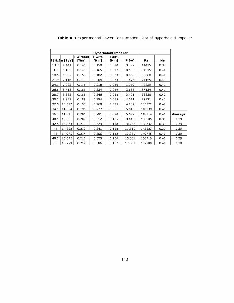
142
Table A.3 Experimental Power Consumption Data of Hyperboloid Impeller
Hyperboloid Impeller
f [Hz] n [1/s] T without [Nm]
T with [Nm]
T diff. [Nm] P [w] Re Ne
13.7 4.441 0.140 0.150 0.010 0.279 44415 0.32
16 5.192 0.148 0.165 0.017 0.555 51915 0.40
18.5 6.007 0.159 0.182 0.023 0.868 60068 0.40
21.9 7.116 0.171 0.204 0.033 1.475 71155 0.41
24.1 7.833 0.178 0.218 0.040 1.969 78329 0.41
26.8 8.713 0.185 0.234 0.049 2.683 87134 0.41
28.7 9.333 0.188 0.246 0.058 3.401 93330 0.42
30.2 9.822 0.189 0.254 0.065 4.011 98221 0.42
32.5 10.572 0.193 0.268 0.075 4.982 105722 0.42
34.1 11.094 0.196 0.277 0.081 5.646 110939 0.41
36.3 11.811 0.201 0.291 0.090 6.679 118114 0.41 Average
40.1 13.051 0.207 0.312 0.105 8.610 130505 0.39 0.39
42.5 13.833 0.211 0.329 0.118 10.256 138332 0.39 0.39
44 14.322 0.213 0.341 0.128 11.519 143223 0.39 0.39
46 14.975 0.214 0.356 0.142 13.360 149745 0.40 0.39
48.2 15.692 0.217 0.373 0.156 15.381 156919 0.40 0.39
50 16.279 0.219 0.386 0.167 17.081 162789 0.40 0.39
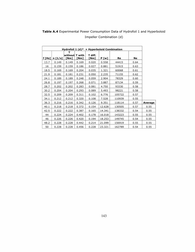
143
Table A.4 Experimental Power Consumption Data of Hydrofoil 1 and Hyperboloid
Impeller Combination (d)
Hydrofoil 1 (d)* + Hyperboloid Combination
f [Hz] n [1/s]
T without [Nm]
T with [Nm]
T diff. [Nm] P [w] Re Ne
13.7 0.149 0.149 0.169 0.020 0.558 44415 0.64
16 0.159 0.159 0.186 0.027 0.881 51915 0.63
18.5 0.169 0.169 0.204 0.035 1.321 60068 0.61
21.9 0.181 0.181 0.231 0.050 2.235 71155 0.62
24.1 0.189 0.189 0.248 0.059 2.904 78329 0.60
26.8 0.197 0.197 0.268 0.071 3.887 87134 0.59
28.7 0.202 0.202 0.283 0.081 4.750 93330 0.58
30.2 0.204 0.204 0.293 0.089 5.493 98221 0.58
32.5 0.209 0.209 0.311 0.102 6.776 105722 0.57
34.1 0.212 0.212 0.320 0.108 7.528 110939 0.55
36.3 0.216 0.216 0.342 0.126 9.351 118114 0.57 Average
40.1 0.218 0.218 0.372 0.154 12.628 130505 0.57 0.55
42.5 0.222 0.222 0.387 0.165 14.341 138332 0.54 0.55
44 0.224 0.224 0.402 0.178 16.018 143223 0.55 0.55
46 0.226 0.226 0.420 0.194 18.253 149745 0.54 0.55
48.2 0.228 0.228 0.442 0.214 21.099 156919 0.55 0.55
50 0.228 0.228 0.456 0.228 23.321 162789 0.54 0.55

144
Table A.5 Experimental Power Consumption Data of Hydrofoil 1 and Hyperboloid
Impeller Combination (1.5d)
Hydrofoil 1 (1.5d)* + Hyperboloid Combination
f [Hz] n [1/s]
T without [Nm]
T with [Nm]
T diff. [Nm] P [w] Re Ne
13.7 4.441 0.135 0.181 0.046 0.039 44415 1.47
16 5.192 0.145 0.195 0.05 0.046 51915 1.17
18.5 6.007 0.156 0.22 0.064 0.063 60068 1.11
21.9 7.116 0.169 0.242 0.073 0.078 71155 0.91
24.1 7.833 0.177 0.258 0.081 0.090 78329 0.83
26.8 8.713 0.183 0.276 0.093 0.107 87134 0.77
28.7 9.333 0.187 0.291 0.104 0.122 93330 0.75
30.2 9.822 0.19 0.3 0.11 0.131 98221 0.72
32.5 10.572 0.195 0.317 0.122 0.149 105722 0.69
34.1 11.094 0.197 0.33 0.133 0.165 110939 0.68
36.3 11.811 0.203 0.346 0.143 0.182 118114 0.64 Average
40.1 13.051 0.206 0.376 0.17 0.220 130505 0.63 0.60
42.5 13.833 0.21 0.395 0.185 0.244 138332 0.61 0.60
44 14.322 0.211 0.41 0.199 0.264 143223 0.61 0.60
46 14.975 0.212 0.43 0.218 0.290 149745 0.61 0.60
48.2 15.692 0.213 0.442 0.229 0.306 156919 0.58 0.60
50 16.279 0.223 0.466 0.243 0.340 162789 0.58 0.60
* Submergence of the top impeller (hydrofoil 1)

145
APPENDIX B
MACROMIXING TIME DATA FOR CYLINDRICAL TANK
MEASUREMENTS
Table B.1 Experimental Macromixing Time Data of 6 Blade Rushton Turbine
6 Blade Rushton Turbine
n [1/min] n [1/s] Mixing time Re n*Mixing Time Average Value
54 0.89 45.54 8940 40.71 38.70 72 1.19 33.83 11920 40.33 38.70 125 2.09 18.78 20860 39.18 38.70 179 2.98 12.62 29800 37.59 38.70 241 4.02 9.33 40230 37.52 38.70 304 5.07 7.34 50660 37.20 38.70 429 7.15 5.36 71520 38.34 38.70
Table B.2 Experimental Macromixing Time Data of Hydrofoil 1 Impeller
Hydrofoil 1 Impeller
n [1/min] n [1/s] Mixing time Re n*Mixing Time Average Value
200 3.33 30.62 33333 102.07 104.2 320 5.33 19.74 53333 105.28 104.2 440 7.33 14.31 73333 104.93 104.2 600 10.00 10.54 100000 105.40 104.2 720 12.00 8.62 120000 103.39 104.2 800 13.33 7.81 133333 104.15 104.2
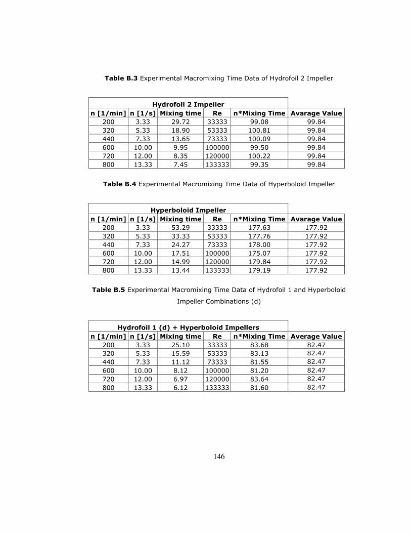
146
Table B.3 Experimental Macromixing Time Data of Hydrofoil 2 Impeller
Hydrofoil 2 Impeller n [1/min] n [1/s] Mixing time Re n*Mixing Time Avarage Value
200 3.33 29.72 33333 99.08 99.84 320 5.33 18.90 53333 100.81 99.84 440 7.33 13.65 73333 100.09 99.84 600 10.00 9.95 100000 99.50 99.84 720 12.00 8.35 120000 100.22 99.84 800 13.33 7.45 133333 99.35 99.84
Table B.4 Experimental Macromixing Time Data of Hyperboloid Impeller
Hyperboloid Impeller n [1/min] n [1/s] Mixing time Re n*Mixing Time Avarage Value
200 3.33 53.29 33333 177.63 177.92 320 5.33 33.33 53333 177.76 177.92 440 7.33 24.27 73333 178.00 177.92 600 10.00 17.51 100000 175.07 177.92 720 12.00 14.99 120000 179.84 177.92 800 13.33 13.44 133333 179.19 177.92
Table B.5 Experimental Macromixing Time Data of Hydrofoil 1 and Hyperboloid
Impeller Combinations (d)
Hydrofoil 1 (d) + Hyperboloid Impellers n [1/min] n [1/s] Mixing time Re n*Mixing Time Average Value
200 3.33 25.10 33333 83.68 82.47 320 5.33 15.59 53333 83.13 82.47 440 7.33 11.12 73333 81.55 82.47 600 10.00 8.12 100000 81.20 82.47 720 12.00 6.97 120000 83.64 82.47 800 13.33 6.12 133333 81.60 82.47
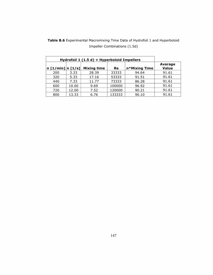
147
Table B.6 Experimental Macromixing Time Data of Hydrofoil 1 and Hyperboloid
Impeller Combinations (1.5d)
Hydrofoil 1 (1.5 d) + Hyperboloid Impellers
n [1/min] n [1/s] Mixing time Re n*Mixing Time Avarage Value
200 3.33 28.39 33333 94.64 91.61 320 5.33 17.16 53333 91.51 91.61 440 7.33 11.77 73333 86.28 91.61 600 10.00 9.69 100000 96.92 91.61 720 12.00 7.52 120000 90.21 91.61 800 13.33 6.76 133333 90.10 91.61

148
APPENDIX C
MACROMIXING TIME DATA FOR SQUARE TANK
MEASUREMENTS
Table C.1 Experimental Macromixing Time Data of Generation 5 Hyperboloid
(Low Rib) Mixer
Generation 5 Hyperboloid Mixer (Low Rib) n [1/min] n [1/s] Mixing time Re n*Mixing Time
160 2.67 191.69 106667 511.17 Average Value 220 3.67 164.35 146667 602.62 583.6 280 4.67 121.24 186667 565.78 583.6 340 5.67 102.78 226667 582.41 583.6
Table C.2 Experimental Macromixing Time Data of Generation 5 Hyperboloid
(High Rib) Mixer
Generation 5 Hyperboloid Mixer (High Rib) n [1/min] n [1/s] Mixing time Re n*Mixing Time
160 2.67 177.09 106667 472.25 Average Value 220 3.67 124.19 146667 455.38 431.9 280 4.67 88.28 186667 411.95 431.9 340 5.67 75.61 226667 428.48 431.9

149
Table C.3 Experimental Macromixing Time Data of Generation 6 Hyperboloid
Mixer
Generation 6 Hyperboloid Mixer n [1/min] n [1/s] Mixing time Re n*Mixing Time
160 2.67 129.50 106667 345.35 Average Value 220 3.67 89.08 146667 326.61 297.8 280 4.67 62.49 186667 291.62 297.8 340 5.67 48.59 226667 275.32 297.8

150
APPENDIX D
AERATION DATA FOR SQUARE TANK MEASUREMENTS
Table D.1 Experimental Aeration Data of Generation 5 (Low Rib) Hyperboloid
Mixer
* Correction curve: 0.0087*x-7.2917
Fl [-] 0.01
n [U/min] 286 382 477 573 QA [Nm^3/h] 1.37 1.83 2.29 2.75 Cond. [µS/cm] 705 861 1020 1181 1340 1500 1655 1812
T(H2O) [°C] 13.6 13.7 13.9 14.1 14.3 14.5 14.7 14.9
kLa [1/h] 9.24 8.92 15.79 16 26.57 26.43 37.3 37.7
OC [kg/h] 36.4 35.2 62.11 62.63 102.86 102.14 144 144 kLa corr.* [1/h] 9.35 8.9 15.54 15.52 25.41 24.91 34.65 34.51 OC corr. [kg/h] 36.82 35.13 61.12 60.76 98.37 96.26 133.77 131.8
8.9 15.54 25.41 34.65
35.13 61.12 98.37 133.77 OA Efficiency [%] 8.56 11.15 14.37 16.27
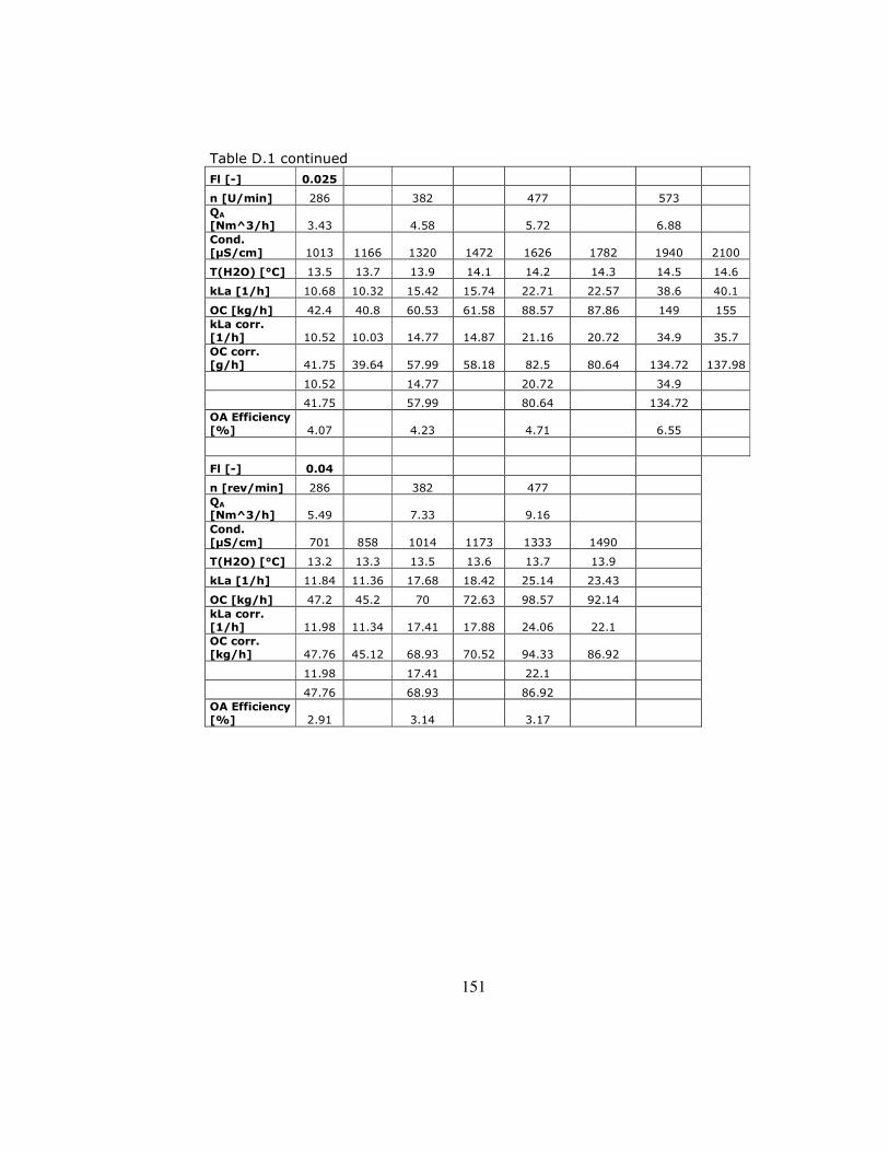
151
Table D.1 continued
Fl [-] 0.025
n [U/min] 286 382 477 573 QA [Nm^3/h] 3.43 4.58 5.72 6.88 Cond. [µS/cm] 1013 1166 1320 1472 1626 1782 1940 2100
T(H2O) [°C] 13.5 13.7 13.9 14.1 14.2 14.3 14.5 14.6
kLa [1/h] 10.68 10.32 15.42 15.74 22.71 22.57 38.6 40.1
OC [kg/h] 42.4 40.8 60.53 61.58 88.57 87.86 149 155 kLa corr. [1/h] 10.52 10.03 14.77 14.87 21.16 20.72 34.9 35.7 OC corr. [g/h] 41.75 39.64 57.99 58.18 82.5 80.64 134.72 137.98
10.52 14.77 20.72 34.9
41.75 57.99 80.64 134.72 OA Efficiency [%] 4.07 4.23 4.71 6.55
Fl [-] 0.04
n [rev/min] 286 382 477 QA [Nm^3/h] 5.49 7.33 9.16 Cond. [µS/cm] 701 858 1014 1173 1333 1490
T(H2O) [°C] 13.2 13.3 13.5 13.6 13.7 13.9
kLa [1/h] 11.84 11.36 17.68 18.42 25.14 23.43
OC [kg/h] 47.2 45.2 70 72.63 98.57 92.14 kLa corr. [1/h] 11.98 11.34 17.41 17.88 24.06 22.1 OC corr. [kg/h] 47.76 45.12 68.93 70.52 94.33 86.92
11.98 17.41 22.1
47.76 68.93 86.92 OA Efficiency [%] 2.91 3.14 3.17

152
Table D.2 Experimental Aeration Data of Generation 6 Hyperboloid Mixer
Fl [-] 0.01
n [rev/min] 286 382 477 573
QA [Nm^3/h] 1.37 1.83 2.29 2.75 Cond. [µS/cm] 915 1070 1226 1383 1542 1697 1854 2010
T(H2O) [°C] 18.4 18.5 18.6 18.7 18.8 18.9 19 19.1
kLa [1/h] 13.3 13.55 21.8 22.2 32.82 33 49.63 50.13
OC [kg/h] 47 47.5 76 77.33 114.55 114.55 172.5 173.75 kLa corr. [1/h] 13.21 13.28 21.06 21.15 30.81 30.53 45.24 45.01 OC corr. [kg/h] 46.69 46.54 73.44 73.67 107.53 105.99 157.25 156.04
13.31 21.15 30.81 45.24
46.69 73.67 107.53 157.25 OA Efficiency [%] 11.37 13.44 15.71 19.12
Fl [-] 0.025
n [rev/min] 286 382 477 573
QA [Nm^3/h] 3.43 4.58 5.72 6.88 Cond. [µS/cm] 1004 1161 1316 1470 1625 1779 1939 2090
T(H2O) [°C] 13.8 14 14.2 14.3 14.5 14.6 14.8 15
kLa [1/h] 14.15 13.75 22.07 22.27 32.18 32.36 53.13 52.75
OC [kg/h] 55.5 53.5 86 86.67 124.55 124.55 203.75 201.25 kLa corr. [1/h] 13.95 13.36 21.15 21.04 29.98 29.71 48.04 47 OC corr. [kg/h] 54.7 52 82.42 81.9 116.02 114.35 184.24 179.33
13.95 21.04 29.71 47
54.7 81.9 114.35 179.33 OA Efficiency [%] 5.33 5.98 6.68 8.72

153
Table D.2 continued Q [-] 0.04
n [rev/min] 286 382 477
QA [Nm^3/h] 5.49 7.33 9.16 Cond. [µS/cm] 860 1016 1172 1330 1484 1641
T(H2O) [°C] 13.3 13.4 13.6 13.8 14 14.1
kLa [1/h] 17.35 16.95 24.07 29.2 40.73 41
OC [kg/h] 69 67 95.33 114.67 159.09 160 kLa corr. [1/h] 17.32 16.69 23.37 27.95 38.44 38.14 OC corr. [kg/h] 68.87 65.96 92.56 109.76 150.15 148.82
17.32 23.37 38.14
68.87 92.56 148.82 OA Efficiency [%] 4.19 4.22 5.43

154
APPENDIX E
ANALYSIS OF TORQUE AND ROTATIONAL SPEED DATA
Torque was measured as 04.0=T Nm for hydrofoil 1 impeller at a rotational
speed of 783 RPM. Following calculations were done to obtain Ne and Re from
these data:
))(60
783(2 rpsπω = (E.1)
rps00.82=ω
ωTP = (E.2)
00.82*04.0=P
28.3=P Watt
35 ** nd
PNe
ρ= (E.3)
( ) ( ) ( )3
3
55
3 60
783*)1.0(*1000
28.3
rpsmm
kg
WattNe
=
15.0=Ne
)(
*Re
2
T
nd
υ= (E.4)
)/(10
))(60/783(*)()1.0(Re
26
22
sm
rpsm−
=
130505Re =

155
APPENDIX F
DISSOLVED OXYGEN MEASUREMENT PROCEDURE
The dissolved oxygen that exists in water is removed before the aeration
measurements by combining it chemically with sodium sulphite according to the
reaction given in Equation F.1.
422322
1SONaOSONa →+ (F.1)
The amount of sodium sulphite required for one experiment depends on the
dissolved oxygen amount in water and on the requirement for a suitable lag time
for admixture. The volume of the tank used in the experiment was 0.365 m3 and
the DO concentration of the tank at 10.8 °C was C =11.08 mg/L. The oxygen
transfer capacity, (the highest OC value ever measured, i.e. the saturation
value of the oxygen solubility) at this temperature was 8.10OC =97.36 g/h =
0.097 kg/h. With a lag time of 15 sec the following is calculated:
Na2SO3 for DO bonding: gkg 32032.08*01108.0*365.0 == (F.2)
Na2SO3 for lag time: gkg 23.300323.08*)3600/15(*097.0 == . (F.3)
So, the total sodium sulphite requirement for one test end in a total of 35.23 g
and to be on the safe side 45 g of sodium sulphite was used for one test
measurement. The amount of water required to dissolve the 45 g of sodium
sulphite was taken from the mixing tank so that exactly the same amount of
water is preserved.

156
The oxidation of sodium sulphite accelerates in the presence of cobalt salt since
it catalyses the reaction. Therefore before beginning the experiment a certain
amount of CoCl2.6H2O was added to ensure a minimum concentration of cobalt
ions in water. 0.2 g of cobalt salt was added before beginning the experiment.
The mixer and the air flow rate were adjusted to required value by the switches
on the right side of the mixing tank.
The process of oxygen saturation is determined with the DO-sensor which was
placed always at the same place, to the left corner of the tank. The signals
coming from the sensor were sent to the measurement amplifier and then to the
interphase card in the PC. The measured signals were visualized in the screen
with the help of a measured data processing program and the ASCII data, where
the concentration value per second, were recorded at the same time.
The aeration is started and the oxygen transfer (absorption) curve is drawn with
the data obtained by the measurements of the oxygen transfer electrodes.
The akL is determined from the slope of the absorption curve through the
program OCA which uses the exponential regression method to obtain the best
fit line to the data.
The increased salt content in water affects the measured values on the basis that
the increasing bubble polarity decreases the normal coalescence. The water in
the tank requires to be changed when a salt content of 2000 mg/L is reached
since this can lead up to a deviation of 10 %. This value can be controlled with a
conductivity measurement probe.
As the oxygen in air dissolve in water, the oxygen amount increases according to
the saturation function:
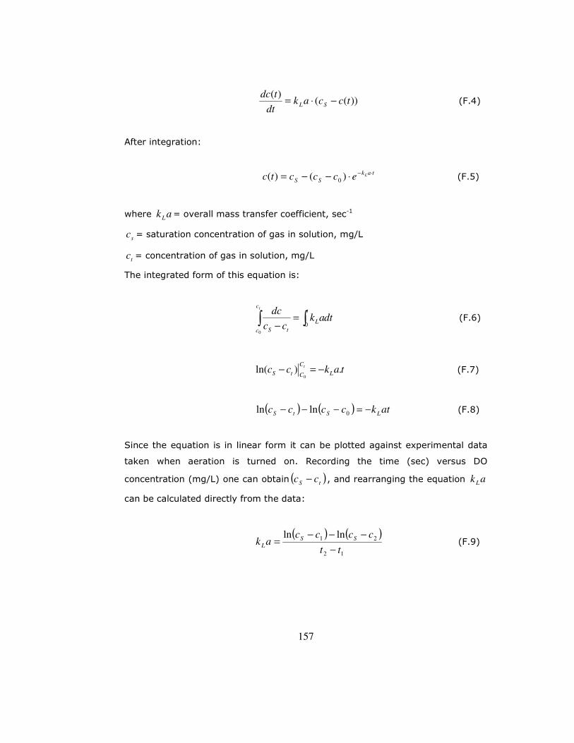
157
))(()(
tccakdt
tdcSL −⋅= (F.4)
After integration:
tak
SSLeccctc
⋅−⋅−−= )()( 0 (F.5)
where akL = overall mass transfer coefficient, sec-1
sc = saturation concentration of gas in solution, mg/L
tc = concentration of gas in solution, mg/L
The integrated form of this equation is:
dtakcc
dctc
c
t
L
tS
∫ ∫=−
0
0 (F.6)
takcc L
C
CtS
t
.)ln(0
−=− (F.7)
( ) ( ) atkcccc LStS −=−−− 0lnln (F.8)
Since the equation is in linear form it can be plotted against experimental data
taken when aeration is turned on. Recording the time (sec) versus DO
concentration (mg/L) one can obtain ( )tS cc − , and rearranging the equation akL
can be calculated directly from the data:
( ) ( )
12
21 lnln
tt
ccccak SS
L−
−−−= (F.9)

158
Drawing the graph of the ( )tS cc −ln versus time and using the slope of the
linear fit to this data one can obtain the overall mass transfer coefficient (oxygen
transfer coefficient), akL in (h-1).
After obtaining the akL , the oxygen transfer capacity in clean water, OC [kg/h]
can be determined. OC is the oxygen supply, that is the mass [kg] of oxygen
transferred by an aeration system in one hour in a tank of certain size filled with
clean water at DO of C =0 mg/L, a water temperature of 20 °C and normal
atmospheric pressure (1013 hPa). The following applies:
1000
20,20 SL cakVOC
∗∗= (F.10)
where
V= Tank volume; 20,Sc =measured DO saturation concentration from the
estimation of a clean water test; 20akL is the oxygen transfer coefficient at clean
water at 20 °C.
Different characteristic numbers provide a comparison between different system
parameters regarding the oxygen transfer efficiency e.g. OCA,h [g/(m3N/m)] and
OAh [%/m] :
1000**
,
wA
hAhQ
OCOC = (F.11)
hAOC , is the specific oxygen supply where AQ is the absorbed air [m3/s] with an
oxygen concentration of 0.299 kg/m3 and wh is the water height [m]. hOA is the
specific oxygen utilization efficiency and defined as follows:

159
)299.0*(*
*100
Aw
hQh
OCOA = (F.12)
For the evaluation of the aeration experiment, the program of the firma
Aquadata was used. The program conforms to the guidelines in ATV-M 209E and
uses the algorithm given above. The program requests the tank volume, the
temperature measured during the experiment and the air injection height ( wh )
of the aerator and the volumetric air flow ( AQ ) as well as the )(tc , t data pair.
The program gives the 20OC value besides the akL value. For the
characterisation of the quality of the measurements, the residues were
calculated by the program and shown graphically. The residues show the
deviation of the each calculated value from the real measured value. A random
distribution of the residues indicates a proper measurement while a waveform
distribution of them means a wrong start of the experiment such as an
incomplete mixing of the tank content or a late sulphide oxidation. By adjusting
the starting time the calculation can be corrected (Frey, 1999).