experimental investigation of twt …aarti/pubs/msthesis_asingh.pdfexperimental investigation of twt...
TRANSCRIPT

EXPERIMENTAL INVESTIGATION OF TWT NONLINEARITIES
AND DISTORTION SUPPRESSION BY SIGNAL INJECTION
Aarti Singh
A thesis submitted in partial fulfillment of the
requirements for the degree of
Master of Science
(Electrical and Computer Engineering)
at the
University of Wisconsin – Madison
2003

i
Acknowledgement
I am indebted to my advisors Prof. J. E. Scharer and Prof. J. H. Booske for the
motivation, support and guidance they have provided for this research. Prof. Scharer’s
expert advising helped me develop a wider perspective to the problem, while paying
equal attention to the intricacies involved. Apart from being a great researcher, Prof.
Scharer is an excellent advisor. I am grateful to him for his caring attitude and
encouragement for both professional and personal development. Prof. Booske is a great
motivator with an admirable zeal for research and exploring new ideas. His advice and
guidance always helped me see clearly through hard problems and experimental issues. I
thank him for all his support.
I also wish to thank my co-researcher and friend, John Wöhlbier who, through the
many discussions we had, helped me develop not only a good understanding but a right
attitude towards research in general. I appreciate his effort and patience in explaining
things over and over and helping me at each step.
I am indebted to Mike Wirth for getting me started on this research work and
always taking out time to help me with both work and personal problems. His invaluable
friendly advice is deeply appreciated.
Mark Converse, Sudeep Bhattacharjee, John Welter and Chad Marchewka, my
co-researchers, have always offered support and advice with lab problems. I thank them
for their cooperation and help.
Last, but not the least, I am indebted to my family for their unselfish nature and
the support and encouragement they provide for everything I wish to achieve.

ii
TABLE OF CONTENTS
Page
LIST OF FIGURES . . . . . . . . . . . . . . . . . . . . . . . . . . . . . . . . . . . . . . . . . . . . . . . . . . . . . . . iv
ABSTRACT . . . . . . . . . . . . . . . . . . . . . . . . . . . . . . . . . . . . . . . . . . . . . . . . . . . . . . . . . . . . . viii
Chapter I – Introduction . . . . . . . . . . . . . . . . . . . . . . . . . . . . . . . . . . . . . . . . . . . . . . . . . . . 1
1.1 Motivation . . . . . . . . . . . . . . . . . . . . . . . . . . . . . . . . . . . . . . . . . . . . . . . . . 1
1.1.1 Nonlinear Distortions . . . . . . . . . . . . . . . . . . . . . . . . . 1
1.1.2 Multitone Problem . . . . . . . . . . . . . . . . . . . . . . . . . . . . 3
1.1.3 Traveling Wave Tube – Nonlinearity considerations . . 4
1.2 Literature Review . . . . . . . . . . . . . . . . . . . . . . . . . . . . . . . . . . . . . . . . . . . 6
1.2.1 TWT Linearization Schemes – Overview . . . . . . . . . . 6
1.2.2 Injection Schemes . . . . . . . . . . . . . . . . . . . . . . . . . . . . 8
1.3 Contribution of this thesis . . . . . . . . . . . . . . . . . . . . . . . . . . . . . . . . . . . . 12
Chapter II – Experimental TWT and Setup . . . . . . . . . . . . . . . . . . . . . . . . . . . . . . . . . . 14
2.1 Experimental tube – the XWING TWT . . . . . . . . . . . . . . . . . . . . . . . . . 14
2.2 NorthStar Power Supply and Control software . . . . . . . . . . . . . . . . . . . . 16
2.3 Vacuum System . . . . . . . . . . . . . . . . . . . . . . . . . . . . . . . . . . . . . . . . . . . . 19
2.4 Solenoid focusing . . . . . . . . . . . . . . . . . . . . . . . . . . . . . . . . . . . . . . . . . . 20
2.5 Current sensing and TWT alignment . . . . . . . . . . . . . . . . . . . . . . . . . . . 21
2.6 XWING start-up Procedure . . . . . . . . . . . . . . . . . . . . . . . . . . . . . . . . . . . 23
2.7 Switching system for output selection . . . . . . . . . . . . . . . . . . . . . . . . . . . 26
2.8 RF Sources and Diagnostic Equipment . . . . . . . . . . . . . . . . . . . . . . . . . . 27
2.9 Experimental Set-up for Suppression using Signal Injection . . . . . . . . . 33
2.10 Discussion of Experimental Errors . . . . . . . . . . . . . . . . . . . . . . . . . . . . . 36
Chapter III – Nonlinear Nature of the Traveling Wave Tube and Characterization . . 38
3.1 Basic Operation . . . . . . . . . . . . . . . . . . . . . . . . . . . . . . . . . . . . . . . . . . . . 38
3.2 Nonlinear Nature and Characterization . . . . . . . . . . . . . . . . . . . . . . . . . . . 39
3.2.1 AM/AM and AM/PM characterization . . . . . . . . . . . . . 40
3.2.2 MUSE (Multi-frequency Spectral Eulerian) model . . . 44
3.3 Experimental characterization of the XWING nonlinearities . . . . . . . . . 48
iii
3.3.1 Gain vs. frequency . . . . . . . . . . . . . . . . . . . . . . . . . . . . 49
3.3.2 Single-tone drive curve characterization . . . . . . . . . . . . 51
3.3.3 Two-tone drive curve characterization . . . . . . . . . . . . . 53
3.3.4 Small-signal Spatial growth-rate characterization . . . . 57
3.3.5 Growth of nonlinear products . . . . . . . . . . . . . . . . . . . . 61
Chapter IV – Signal Injection schemes for TWT Linearization . . . . . . . . . . . . . . . . . . . 68
4.1 Physics of Signal Injection in a TWT amplifier . . . . . . . . . . . . . . . . . . . 68
4.2 Second-harmonic Suppression by Second-harmonic Injection . . . . . . . . 71
4.3 Fundamental Enhancement by Second-Harmonic Injection . . . . . . . . . . 77
4.4 3IM Suppression by Second-harmonic Injection . . . . . . . . . . . . . . . . . . . 82
4.5 3IM Suppression by IM3 Injection . . . . . . . . . . . . . . . . . . . . . . . . . . . . . 90
4.6 Sensitivity of the Injection schemes . . . . . . . . . . . . . . . . . . . . . . . . . . . . . 93
4.7 3IM Suppression by Two-frequency (3IM + Second-Harmonic)
Injection . . . . . . . . . . . . . . . . . . . . . . . . . . . . . . . . . . . . . . . . . . . . . . . . . 95
4.8 Bandwidth of Suppression . . . . . . . . . . . . . . . . . . . . . . . . . . . . . . . . . . . 99
4.9 Comparison of the schemes . . . . . . . . . . . . . . . . . . . . . . . . . . . . . . . . . . 100
Chapter V – Summary . . . . . . . . . . . . . . . . . . . . . . . . . . . . . . . . . . . . . . . . . . . . . . . . . . . . 103
5.1 Conclusion . . . . . . . . . . . . . . . . . . . . . . . . . . . . . . . . . . . . . . . . . . . . . . . 103
5.2 Future Work . . . . . . . . . . . . . . . . . . . . . . . . . . . . . . . . . . . . . . . . . . . . . . 106
APPENDICES
Appendix A XWING TWT Specifications . . . . . . . . . . . . . . . . . . . . . . . . . . . . . . 109
Appendix B Tap Coupling measurements . . . . . . . . . . . . . . . . . . . . . . . . . . . . . . 110
Appendix C Computer control of NorthStar - Troubleshooting and Blanking . . . 112
Signal Generation
Appendix D Suggestions on gate-valve mechanism improvement. . . . . . . . . . . . 115
Appendix E Cathode Conditioning Procedure. . . . . . . . . . . . . . . . . . . . . . . . . . . 117
Appendix F Flexible and semi-rigid coax cable losses. . . . . . . . . . . . . . . . . . . . . 118
Appendix G Amplitude Correction Table for Output and Tap path. . . . . . . . . . . . 119
REFERENCES . . . . . . . . . . . . . . . . . . . . . . . . . . . . . . . . . . . . . . . . . . . . . . . . . . . . . . . . . . .120
iv
LIST OF FIGURES
Figure Page
1.1 Spectral distortion produced by a nonlinear system for (a) single-tone (b) multi- tone inputs. . . . . . . . . . . . . . . . . . . . . . . . . . . . . . . . . . . . . . . . . . . . . . . . . . . . . . . . . 1-2
1.2 In Communication applications, spectral regrowth causes (a) In-band distortion and (b) Cross-talk. . . . . . . . . . . . . . . . . . . . . . . . . . . . . . . . . . . . . . . . . . . . . . . . . . . . . 2
1.3 Multiple-access techniques that maximize time-frequency space utilization. . . . . . . . 3
1.4 Close carrier spacing in techniques like OFDM necessitates need to contain spectral regrowth due to nonlinear distortions. . . . . . . . . . . . . . . . . . . . . . . . . . . . . . . 4
1.5 Prevalent linearization schemes: (a) Predistortion (b) Feedback and (c) Feed- forward linearization. . . . . . . . . . . . . . . . . . . . . . . . . . . . . . . . . . . . . . . . . . . . . . . . . 6-7
1.6 Block diagram of LINC architecture for linearizing TWT response. . . . . . . . . . . . . . 7
2.1 Experimental device – the custom-modified research TWT, XWING. . . . . . . . . . . . 14
2.2 Schematic diagram of the XWING tube assembly. . . . . . . . . . . . . . . . . . . . . . . . . . . 15
2.3 Picture of (a) the LabView Interface (b) the NorthStar pulse modulator. . . . . . . . . . 16
2.4 Oscilloscope trace showing cathode voltage pulse (trace 1, scale 1V:1kV) and synchronized TTL pulse (trace 4). . . . . . . . . . . . . . . . . . . . . . . . . . . . . . . . . . . . . . . . 18
2.5 Vacuum system configuration for XWING. . . . . . . . . . . . . . . . . . . . . . . . . . . . . . . . 19
2.6 Solenoid magnet focusing for the electron beam. The XWING is placed at the centre of the solenoids. . . . . . . . . . . . . . . . . . . . . . . . . . . . . . . . . . . . . . . . . . . . . . . . . . . . . . 20
2.7 (a) Solenoid positions and optimum current values (b) Measured axial magnetic field profile for XWING. . . . . . . . . . . . . . . . . . . . . . . . . . . . . . . . . . . . . . . . . . . . . . . 21
2.8 High-voltage distribution box with cathode, collector current sensors and high- voltage cathode pulse connections to the tube. . . . . . . . . . . . . . . . . . . . . . . . . . . . . . 22
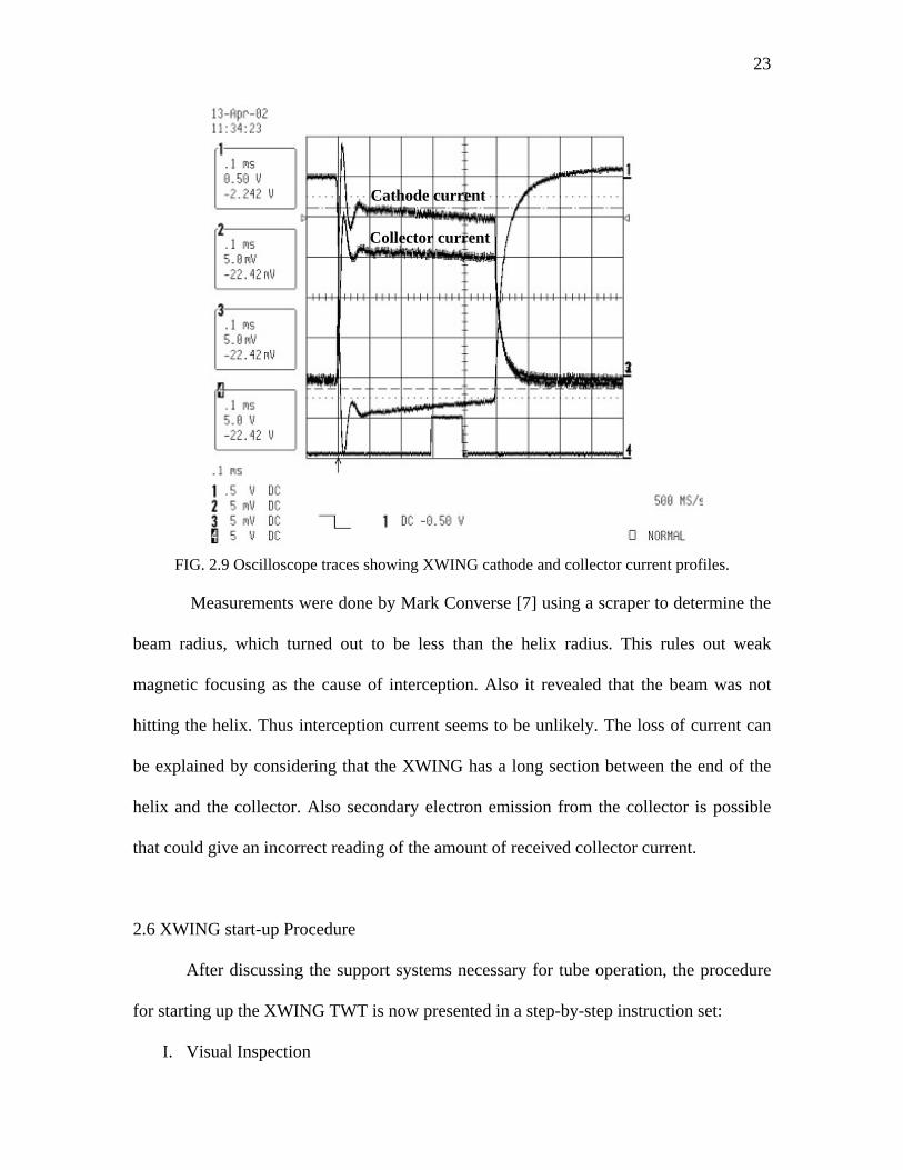
2.9 Oscilloscope traces showing XWING cathode and collector current profiles. . . . . . 23
2.10 (a) Schematic of output switching network (b) Picture of switching assembly and (c) Switch control board. . . . . . . . . . . . . . . . . . . . . . . . . . . . . . . . . . . . . . . . . . . . 26-27
2.11 Photo of primary laboratory RF diagnostic equipment. . . . . . . . . . . . . . . . . . . . . . . . 28
2.12 Output power (trace 4) and hence gain variation over the pulse duration due to voltage droop at 4 GHz. . . . . . . . . . . . . . . . . . . . . . . . . . . . . . . . . . . . . . . . . . . . . . . . 30
2.13 Block diagram of a time-gated spectrum analyzer. . . . . . . . . . . . . . . . . . . . . . . . . . . . 31
2.14 Experimental set-up for XWING linearization using simultaneous injection of second-harmonic and 3IM along with the two fundamental drive tones. . . . . . . . . . . 33
3.1 Simple diagram of the TWT structure. . . . . . . . . . . . . . . . . . . . . . . . . . . . . . . . . . . . . 37

v
3.2 Formation of electron bunches (color shows the intensity of the bunches) and growth of EM wave. . . . . . . . . . . . . . . . . . . . . . . . . . . . . . . . . . . . . . . . . . . . . . . . . . 38
3.3 Nonlinear characterization of an amplifier using (a) Amplitude distortion A[r(t)] curve or AM/AM curve (b) Phase distortion ∆Ф[r(t)] curve or AM/PM curve. . . . . 39
3.4 Voltage transfer curves (a) AM/AM (odd-function) and (b) AM/PM (even function) . . . . . . . . . . . . . . . . . . . . . . . . . . . . . . . . . . . . . . . . . . . . . . . . . . . . . . . . . . . 41
3.5 Circuit voltage and electron beam current showing presence of harmonic content in the beam prior to voltage saturation. (Simulations done using IBC code). . . . . . . 43
3.6 MUSE simulation showing that harmonic generation, and not dc reduction of beam velocity, is the primary cause of phase distortion in TWTs. . . . . . . . . . . . . . . 46
3.7 (a) Phase evolution of the wave for two different input power levels, and (b) Spatial evolution of the beam velocity for the same power levels. . . . . . . . . . . . 46
3.8 Characterization of XWING Gain vs. frequency for three input powers: -10, 0 and 15 dBm. . . . . . . . . . . . . . . . . . . . . . . . . . . . . . . . . . . . . . . . . . . . . . . . . . . . . . . . . . . . 48
3.9 Small-signal gain comparison of the XWING TWT. . . . . . . . . . . . . . . . . . . . . . . . . . 49
3.10 Single-tone drive curve (AM/AM) characterization of the XWING TWT. . . . . . . . . 50
3.11 Drive curves for 4 GHz as input and 4 GHz as second-harmonic with 2 GHz drive. The curves show that same frequency (4 GHz) has different growth rates as a second-order product and as a driven term. . . . . . . . . . . . . . . . . . . . . . . . . . . . . . . . . 52
3.12 Two-tone drive-curve characterization of (a) Output power vs. input power (b) Gain vs. input power for 50 MHz spacing between the tones (1.95 GHz and 2.00 GHz). . . . . . . . . . . . . . . . . . . . . . . . . . . . . . . . . . . . . . . . . . . . . . . . . . . . . . . 53
3.13 Comparison of drive curves for single-tone input at 2.00 GHz and total power in the two fundamentals for a two-tone input at 1.95 and 2.00 GHz. . . . . . . . . . . . . . . 54
3.14 Two-tone drive-curve characterization of (a) Output power vs. input power (b) Gain vs. input power for 500 MHz spacing between the tones (2.00 GHz and 2.50 GHz). . . . . . . . . . . . . . . . . . . . . . . . . . . . . . . . . . . . . . . . . . . . . . . . . . . . . . . 55
3.15 Comparison of two-tone drive curves with 50 MHz and 500 MHz spacing between the carriers. . . . . . . . . . . . . . . . . . . . . . . . . . . . . . . . . . . . . . . . . . . . . . . . . . . . . . . . . . 56
3.16 Single-tone spatial growth-rate of frequencies in the XWING TWT for small-signal 0 dBm drive. . . . . . . . . . . . . . . . . . . . . . . . . . . . . . . . . . . . . . . . . . . . . . . . . . . . . . 57-58
3.17 Harmonic growth-rate for fundamental drives of (a) 1 GHz, (b) 2 GHz and (c) 3 GHz. . . . . . . . . . . . . . . . . . . . . . . . . . . . . . . . . . . . . . . . . . . . . . . . . . . . . . . . 59-60
3.18 Evolution of harmonic distortion with input power. . . . . . . . . . . . . . . . . . . . . . . . . . 61
3.19 Spatial evolution of second-harmonic for 2 GHz, 15 dBm drive. (Note that the spacing shown between the taps shown here is only representative and not the actual distance). . . . . . . . . . . . . . . . . . . . . . . . . . . . . . . . . . . . . . . . . . . . . . . . . . . . . . 61
vi
3.20 Output spectrum of the XWING for two-tone excitation at 1.90 and 1.95 GHz and drive levels of 15 and 18 dBm/tone. . . . . . . . . . . . . . . . . . . . . . . . . . . . . . . . . . . . . . 62
3.21 Spatial evolution of nonlinear distortion components for two-tone excitation at 1.90 and 1.95 GHz with 15 dBm/tone. . . . . . . . . . . . . . . . . . . . . . . . . . . . . . . . . . . . . . . . . . . . . . . . . . 63-64
3.22 Comparison of Experimental measurements for spatial evolution of nonlinear products with LATTE simulations. . . . . . . . . . . . . . . . . . . . . . . . . . . . . . . . . . . . . . . . . . . . . . . . . . . . . . 65-66
4.1 Earlier hypothesis of mechanism of cancellation by harmonic injection. Similar to Fig. 4 of Ref. [13]. In this view, the injected harmonic cancels the nonlinearly
generated harmonic at all positions along the TWT. . . . . . . . . . . . . . . . . . . . . . . . . . . . . . . . . . . . . . 68
4.2 Illustration of second harmonic suppression by second harmonic injection in a TWT using the analytic solution given in Eq. (4.3). Destructive interference of the driven and nonlinear harmonic wave modes results in cancellation of the total solution at a single axial location. The two modes and their sum is shown in (a) on a linear scale while (b) shows component and sum envelope magnitudes on a log scale. . . . . . . . . . . . . . . . . . . . . . . . . . . . . . . . . . . . . . . . . . . 71-72
4.3 Experimentally observed suppression of second harmonic by 28.8 dB by second- harmonic injection. The fundamental input was kept at 2 GHz, 15 dBm while the injected harmonic at 4 GHz was varied in amplitude and phase to obtain maximum suppression. . . . . . . . . . . . . . . . . . . . . . . . . . . . . . . . . . . . . . . . . . . . . . . . . . . . . . . . . 73
4.4 Experimental and numerical evolution of second-harmonic (a) without injection, (b) with harmonic injection obtaining 29 dB suppression at output, and (c) with harmonic injection obtaining 31 dB suppression at sensor 4. . . . . . . . . . . . . . . . . . . 74
4.5 Variation of output fundamental and harmonic power with second-harmonic injection depicted on (a) log scale and (b) linear scale showing that second-harmonic injection provides not only suppression of the second-harmonic but also improves the fundamental output. . . . . . . . . . . . . . . . . . . . . . . . . . . . . . . . . . . . . . . . . . . . . . . . 77
4.6 Harmonic suppression and fundamental enhancement at XWING output for 1.5 GHz, 15 dBm drive on (a) log scale and (b) linear scale. . . . . . . . . . . . . . . . . . . . . . 79
4.7 Harmonic suppression and fundamental enhancement at sensor 1 of XWING for 2.0 GHz, 15 dBm drive on (a) log scale and (b) linear scale. (Note: The axes for fundamental and harmonic power levels are separate due to smaller levels of harmonic at sensor 1). . . . . . . . . . . . . . . . . . . . . . . . . . . . . . . . . . . . . . . . . . . . . . . . . 80
4.8 Envelope magnitudes of the injected and nonlinear component modes, and total solution for 3IM suppression by harmonic injection. . . . . . . . . . . . . . . . . . . . . . . . . 82
4.9 Output spectra without and with optimum injection of upper second-harmonic to suppress upper 3IM for fundamental inputs of 15dBm/tone. . . . . . . . . . . . . . . . . . . 84
4.10 Output spectra without and with optimum injection of upper second-harmonic to suppress upper 3IM for fundamental inputs of 18dBm/tone. . . . . . . . . . . . . . . . . . . 85
4.11 Spatial evolution of the relevant spectral frequencies at (a) sensor 1, (b) sensor 4, (c) sensor 5, (d) sensor 6 and (e) output for harmonic injection to suppress upper

vii
3IM. . . . . . . . . . . . . . . . . . . . . . . . . . . . . . . . . . . . . . . . . . . . . . . . . . . . . . . . . . . . 86-87
4.12 Spatial evolution of frequency spectrum along TWT axis for suppression of both 3IMs by injection of second-harmonics. . . . . . . . . . . . . . . . . . . . . . . . . . . . . . . . 87-88
4.13 Envelope magnitudes of the injected and nonlinear component modes, and total solution for 3IM suppression by 3IM injection. . . . . . . . . . . . . . . . . . . . . . . . . . . . . 90
4.14 Output spectra without and with optimum injection of upper 3IM frequency to suppress upper 3IM for fundamental inputs of 15dBm/tone. . . . . . . . . . . . . . . . . . . 91
4.15 Output spectra without and with optimum injection of upper second-harmonic to suppress upper 3IM for fundamental inputs of 18dBm/tone. . . . . . . . . . . . . . . . . . . 92
4.16 Sensitivity of suppression of signal injection to injected amplitude and phase. The case shown here is for second-harmonic injection for fundamentals 1.90 and 1.95 GHz at 18 dBm/tone. . . . . . . . . . . . . . . . . . . . . . . . . . . . . . . . . . . . . . . . . . . . . . . . . . 93
4.17 Phasor diagram at TWT output for the different modes in a two-frequency (3IM + second-harmonic) injection scheme. The resultant of the two modes due to injected harmonic and 3IM can cancel the naturally produced 3IM by adjusting the length or amplitude of the phasors as long as the phase of the two injected modes lie above the dashed line. . . . . . . . . . . . . . . . . . . . . . . . . . . . . . . . . . . . . . . . . . . . . . . . . 95
4.18 Output spectra without and with simultaneous injection of upper second-harmonic and upper 3IM to suppress upper 3IM by adjusting injected amplitudes only. . . . . . 96
4.19 Spatial evolution of upper 3IM with simultaneous injection of second-harmonic and upper 3IM frequency at 15 dBm/tone obtaining 30.5 dB suppression at the output. . . . . . . . . . . . . . . . . . . . . . . . . . . . . . . . . . . . . . . . . . . . . . . . . . . . . . . . . . . . . 97
4.20 Simulation results confirming that two-frequency injection can be used to suppress a distortion product by adjusting only injected amplitudes and eliminates precise phase control required by other techniques. . . . . . . . . . . . . . . . . . . . . . . . . . . . . . . . 97
4.21 Sensitivity of upper 3IM suppression to lower fundamental frequency variation for second-harmonic injection scheme. Injection was optimized for fa = 1.90 GHz. . . . 98
4.22 Spatial evolution of 3IM for harmonic injection and two-frequency injection schemes for 3IM suppression optimized at output. . . . . . . . . . . . . . . . . . . . . . . . . . 101
B.1 Frequency dependent coupling loss between output and (a) Tap 1, (b) Tap 4, (c) Tap 5 and (d) Tap 6. . . . . . . . . . . . . . . . . . . . . . . . . . . . . . . . . . . . . . . . . . . 109-110
C.1 PCB Circuit used for generating external Blanking signal. . . . . . . . . . . . . . . . . . . . 113
D.1 A possible circuit to improve gate-valve and turbo closing scheme. . . . . . . . . . . . 114
F.1 Dispersion loss characterization of (a) 3 ft. flexible and (b) semi-rigid coax. . . . . 117
G.1 Frequency dependent losses of output path and tap path. . . . . . . . . . . . . . . . . . . . . 118

viii
Abstract
Traveling Wave Tube (TWT) amplifiers are high power, often broadband
microwave amplifiers used extensively in satellite communications and electronic
countermeasures. While the high-power outputs and wide gain-bandwidths make TWTs
ideally suited for these purposes, the nonlinearity of these devices results in amplitude,
phase and spectral distortion. Nonlinear distortion products appear as harmonics and for
multi-carrier operation also as intermodulation products, at the output of the amplifier
thus limiting the usable bandwidth of the amplifier and degrading fundamental efficiency.
This spectral growth also causes spill-over of one channel’s signal into adjacent
frequency channels, as well as distorts the signal within the same frequency band causing
inter-symbol interference. Thus, suppression of harmonics and intermodulation
frequencies in the output spectra of TWT amplifiers is desirable for reliable and high
data-rate multi-carrier communication.
This thesis presents an experimental investigation of the nonlinear behavior of a
traveling wave tube amplifier. Preliminary computational modeling results are also
shown using the LATTE/MUSE/S-MUSE numerical suite. This understanding is crucial
to develop and explore linearization techniques for the TWT. In particular, signal
injection schemes are investigated for suppressing nonlinear distortion products eg.
Second-harmonic suppression by second-harmonic injection and third-order
intermodulation suppression by injection of second-harmonic or/and third-order
intermodulation frequency. It is shown that by injecting a small amount (15 dBc or less)
of properly phased harmonic or intermod signal at the input, the TWT nonlinearity can be
utilized to suppress the distortion signal produced naturally at the output. Experimental
ix
evidence is provided to support a new understanding of the physical mechanism
responsible for suppression by signal injection. The concepts examined and
experimentally measured open the possibility to develop several related schemes for
distortion suppression in TWT amplifiers and have an enormous potential to enhance
efficiency, bandwidth and data-rates for satellite communication and electronic
countermeasure applications.
1
Chapter I
Introduction
1.1 Motivation
Traveling Wave Tubes (TWTs) are microwave amplifiers widely used in satellite
communication (as broadcast amplifiers) and electronic countermeasures or ECM (for
radar jamming and spoofing). While these amplifiers remain unmatched in their high-
power capabilities and broad gain-bandwidths, the nonlinearity of these devices has been
a limiting factor. This section describes the distortions induced by a nonlinear amplifier,
the linearity requirements of current multi-tone modulation techniques and the limitations
imposed by TWT nonlinearity in its use for communication and ECM applications.
1.1.1 Nonlinear Distortions
Nonlinear amplification of a signal leads to spectral distortion that also results in
amplitude and phase deformation. Spectral regrowth occurs in the form of harmonics and
intermodulation products (IMPs) and thus distorts the output spectrum of the amplified
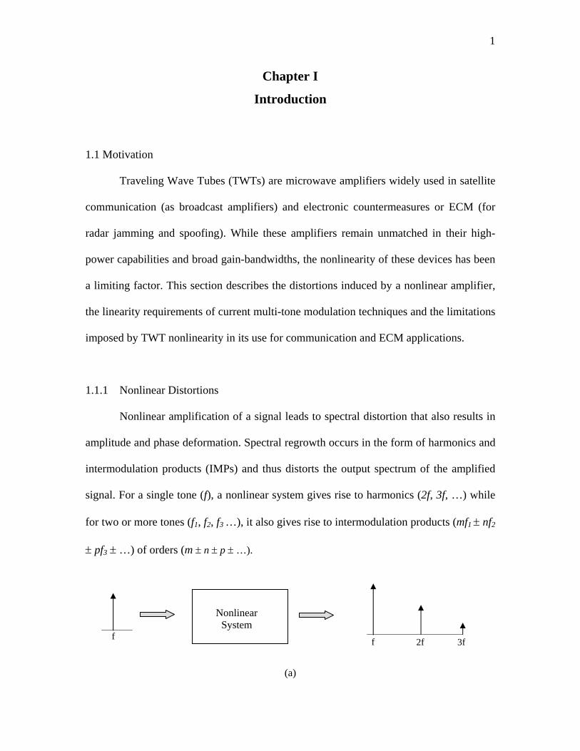
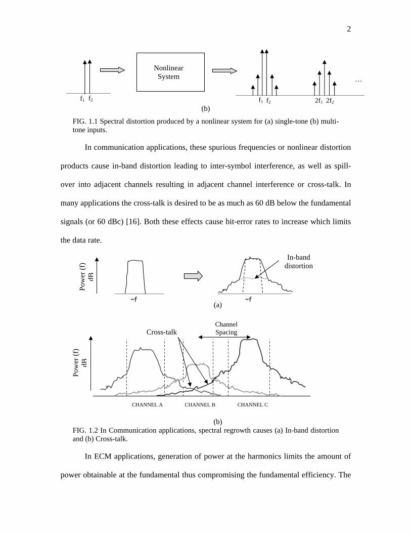
signal. For a single tone (f), a nonlinear system gives rise to harmonics (2f, 3f, …) while
for two or more tones (f1, f2, f3 …), it also gives rise to intermodulation products (mf1 ± nf2
± pf3 ± …) of orders (m ± n ± p ± …).
(a)
f f 2f 3f
NonlinearSystem
2
(b)
FIG. 1.1 Spectral distortion produced by a nonlinear system for (a) single-tone (b) multi-tone inputs.
In communication applications, these spurious frequencies or nonlinear distortion
products cause in-band distortion leading to inter-symbol interference, as well as spill-
over into adjacent channels resulting in adjacent channel interference or cross-talk. In
many applications the cross-talk is desired to be as much as 60 dB below the fundamental
signals (or 60 dBc) [16]. Both these effects cause bit-error rates to increase which limits
the data rate.
(a)
(b)
FIG. 1.2 In Communication applications, spectral regrowth causes (a) In-band distortion and (b) Cross-talk.
In ECM applications, generation of power at the harmonics limits the amount of
power obtainable at the fundamental thus compromising the fundamental efficiency. The
CHANNEL A CHANNEL B CHANNEL C
Channel Spacing Cross-talk
f1 f2 f1 f2
…
2f22f1
NonlinearSystem
~f ~f
In-band distortion
Pow
er (f
) dB
Pow
er (f
) dB

3
TWT is generally operated at or close to saturation to provide maximum power output.
However, spectral regrowth becomes more pronounced as the amplifier is driven harder
and this requires the tube to be operated a few dB “backed-off” from saturation to reduce
nonlinear effect, thus compromising device efficiency.
1.1.2 Multitone Problem
While it is possible to filter out the harmonic content, the intermodulation
products around the fundamental are too close to be filtered out without affecting the
fundamental. Thus nonlinear effects impose a greater problem for multi-tone excitation.
However, multi-carrier operation is indispensable for high data rate and secure
communications.
High data rate implies high bandwidth and since the available bandwidth is
limited, the goal is to pack as many users as possible in the same frequency band by
multiplexing them in time (TDMA – Time Division Multiple Access), frequency (FDMA
– Frequency Division Multiple Access) or both (FH-CDMA – Frequency Hopping Code
Division Multiple Access) [23].
FIG. 1.3 Multiple-access techniques that maximize time-frequency space utilization.
The need to pack many users in same frequency band causes even closer carrier spacing
and thus distortion due to intermodulation products becomes more pronounced.
TDMA time
band
wid
th
1 2 … N
FDMA
time
band
wid
th 1 2 … N
time
band
wid
th
FH-CDMA

4
Techniques like Orthogonal Frequency-Division Multiplexing (OFDM) overlap the user
spectra by placing the carriers orthogonally, imposing more demands on linearity.
FIG. 1.4 Close carrier spacing in techniques like OFDM necessitates need to contain spectral regrowth due to nonlinear distortions.
Spread spectrum (DSSS-CDMA – Direct Sequence Spread Spectrum Code
Division Multiple Access) and pseudo-noise signaling techniques for ECM and covert
communications use a broadband signal that has multiple frequency content. Thus
operation of an amplifier under multi-tone excitation is necessary even in this case.
Modulation techniques like OFDM and CDMA tend to have high peak-to-average
power ratios (PAR) due to phasing effects between multiple signals. This high PAR
causes amplifier to go into saturation frequently and requires the amplifier’s operation at
more backoff from saturation. The problem is aggravated even further since multiple
carrier operation causes saturation to occur at lower drive levels and thus needs even
more backoff, compromising the device efficiency. This issue is discussed in more detail
in Chapter 3.
1.1.3 Traveling Wave Tube – Nonlinearity considerations
Satellite communication requires high power amplification of the signals at the
satellite repeater/broadcast amplifier to overcome the losses encountered by the signal in
OFDM spectra
Channel BW
f
5
traversing the atmosphere. Also it requires using minimum number of amplifiers to keep
the cost and weight at the satellite low. TWTs offer high power outputs and also broader
bandwidths of amplification, implying amplification of many channels using one
amplifier. Thus, TWTs are well-suited for satellite communications. However, with the
limited frequency spectrum available and the ever-increasing demand for more and more
channels, communication systems are now desired to transmit as many channels as
possible in an allocated frequency band. This requires communication amplifiers to have
minimum nonlinearity to reduce spectral regrowth and spilling into adjacent channels.
In ECM or Electronic CounterMeasure applications, spoofing for enhanced
security requires using spread spectrum (eg. Frequency hopping) and pseudo-noise
signaling techniques that need broadband amplifiers. Also high-power is desired for radar
jamming. While TWTs are ideally suited for these applications too, nonlinearity limits
the usable bandwidth of these devices, particularly when the harmonics of the signal
being amplified lie within the gain-bandwidth of the amplifier, compromising the
fundamental efficiency.
One way to reduce the amplifier’s nonlinear effects is to operate the amplifier
backed-off from saturation. However, this limits the maximum output power available
and compromises the device’s power efficiency. Thus, linearization of TWT amplifiers is
necessary for improving both the spectral efficiency and power efficiency of these
devices.
6
1.2 Literature Review
This section provides an overview of linearization schemes for a Traveling Wave
Tube amplifier. It also presents in some detail a review of the literature and progress
made in investigating signal injection schemes.
1.2.1 TWT Linearization Schemes - Overview
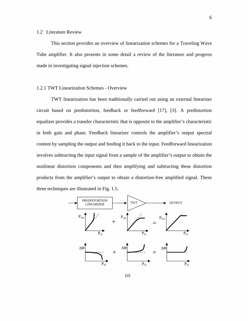
TWT linearization has been traditionally carried out using an external linearizer
circuit based on predistortion, feedback or feedforward [17], [3]. A predistortion
equalizer provides a transfer characteristic that is opposite to the amplifier’s characteristic
in both gain and phase. Feedback linearizer controls the amplifier’s output spectral
content by sampling the output and feeding it back to the input. Feedforward linearization
involves subtracting the input signal from a sample of the amplifier’s output to obtain the
nonlinear distortion components and then amplifying and subtracting these distortion
products from the amplifier’s output to obtain a distortion-free amplified signal. These
three techniques are illustrated in Fig. 1.5.
(a)
PREDISTORTION LINEARIZER TWT OUTPUT
∆Φ ∆Φ
Pin
∆Φ
Pin
Pout
=
Pout
Pout
Pin
Pin Pin
+
+ =
Pin
7
(b) (c)
FIG. 1.5 Prevalent linearization schemes: (a) Predistortion (b) Feedback and (c) Feedforward linearization.
A lot of literature is available on these techniques, including references of [17],
[3]. Some other techniques and variations include adaptive predistortion, envelope
estimation and restoration and Cartesian feedback.
Another technique called LInear amplification using Nonlinear Components
(LINC) has been proposed and is of current interest [6], [8]. LINC involves separating the
input signal into two constant-amplitude signals that can be amplified distortion-free by
two identical nonlinear amplifiers and then combined together to get an amplified version
of the input signal.
FIG. 1.6 Block diagram of LINC architecture for linearizing TWT response.
A novel linearization technique [5] has been recently proposed for TWTs that is
based on the physics of the device. It involves varying the beam energy/velocity by
modulating the cathode or helix voltage and beam current by varying the grid or focus
electrode voltage, using direct feed or feedback loop to compensate for nonlinear
distortion.
TWT
FEEDBACK NETWORK
TWT φ Σ
φ Σ
+
+-
-
+
QMOD
QMOD
+
Baseband Input
Constant amplitude signal Component
Separator
Frequency up-conversion
Matched TWT
amplifiers
Power combiner
8
While many of these techniques have been widely used for TWT linearization,
they are plagued with various issues. Predistortion requires a good estimate of the
amplifier’s amplitude and phase characteristics over the device bandwidth and tuning to
match these parameters. Also predistortion equalizers designed to suppress lower order
intermods, are known to aggravate the higher order distortion products. This is discussed
further in Chapter 4. Feedback, feedforward and helix voltage modulation schemes suffer
from bandwidth limitations due to delays in lines and feedback loops as well as stability
and drift problems. LINC on the other hand requires matched modulators and amplifiers.
Also signal separation and low loss, high isolation power combining is difficult. This
necessitates the need for exploring more linearization techniques that are simple,
broadband and provide more effective linearization. This thesis investigates various
signal injection techniques and evaluates their performance in suppressing nonlinear
distortions.
1.2.2 Injection Schemes
Signal injection techniques involve conditioning the spectra at the output of the
amplifier by injecting signal(s) of proper amplitude and/or phase to cancel nonlinear
distortion product(s). While many signal injection schemes have been proposed for solid-
state amplifiers, their application to traveling wave tubes has not been completely
explored and understood.
Harmonic generation in broadband TWTs was investigated by Dionne [9] who
observed that “Tubes which are driven by a signal with appreciable harmonic content …
have an output performance which varies widely depending on the phase of the input

9
signals.” He further explained using simulations that the input second harmonic phase
can either cause premature deceleration and hence early saturation, or assist the beam
bunching leading to efficiency improvement. This phenomenon where the wrong-type of
injected second-harmonic input could seriously degrade the power output at the
fundamental frequency, while correct amount of a properly-phased second-harmonic will
increase the fundamental power output and suppress the second harmonic at the output of
the tube, became widely known. Based on Dionne’s work, Hamilton and Zavadil [15]
developed a “Harmonically-Enhanced Two-Octave TWT” that used a gain equalizer and
phase compensator to condition and inject a harmonic signal from a driver TWT. For the
lower frequencies, this resulted in increased fundamental power and suppression of
harmonics to 8 dB or more below the fundamentals.
The first hypothesis for the physical mechanism of suppression by harmonic
injection was given by Mendel [18]. He suggested that harmonic injection can be
described as a process of cancellation “…whereby the injected second-harmonic signal is
such that it is 180° out of phase with the second harmonic signal generated by the
nonlinear processes inherent in the interaction mechanism.”
This view was supported by Garrigus and Glick [13] who state “If a second
harmonic wave of proper amplitude and phase … were to be injected at the input of the
amplifier, it would minimize the harmonic developed in the tube …” and even speculated
what the harmonic signal components might look like internal to the TWT. They report a
9 dB increase in power output with harmonic conditioning at the low end of the gain-
bandwidth. Their sensitivity studies reveal that varying the input phase by 30-60° and the

10
input amplitude by 2-3dB resulted in only 1 dB loss in power output. Ref. [13] also
presents guidelines for designing a harmonic conditioner.
Suppression of third-order intermods (3IMs) by second harmonic injection in a
TWT was demonstrated by Sauseng et al [25]. A backed off wideband driver tube was
used to generate the injected harmonic signals and improvements of upto 6-7 dB were
reported at saturation for two-tone input. For four-tone input at saturation, a reduction of
3-7 dB in third-order intermodulation as well as 5-13 dB reduction in second harmonics
and second-order intermodulation were reported. Also the fundamental signals were
boosted by 3.5 dB. Thus, unlike predistortion linearizer, harmonic injection appears to
suppress all nonlinear products. Sauseng et al. also investigated the dynamic range of
intermodulation improvement. They claim that improvement can be achieved about ±6dB
from the optimized drive level and that amount of suppression obtained changes by
roughly 3dB/dB. They also state that reoptimizing injection at a different drive level
yields approximately the same intermodulation distortion improvement. It should be
noted that varying the drive level changes both the fundamental and second harmonic
input power. In Ref. [25], Sauseng et al. state that “One would expect that the second
harmonic contents of the beam modulation become significantly reduced with harmonic
injection.” However, they observed that large signal analysis predicts that such harmonic
reduction of the beam modulation is not very pronounced and occurs close to saturation
(where the injection was optimized). In Section 4.1, we provide an explanation for their
seemingly contradictory results.
Recently, suppression of up to 24 dB was reported in a paper by M. Wirth et al.
[27, 28] for second harmonic injection to suppress 3IM. Sensitivity studies of suppression

11
for injected amplitude and phase levels indicate an increase in harmonic power by
~7dB/dB and ~7dB/5° deviation from optimum amplitude and phase. This higher
sensitivity compared to that reported in [13, 25] is expected due to increase in the amount
of suppression obtained. Also it was observed that higher suppression is obtained when
the device is operated closer to saturation, as against Ref. [25]. However, it should be
noted that the amount of suppression recorded in [25] was much less than the amount of
suppression reported in [28].
Work by Dionne [9] and later by Datta et al. [10, 11] predicted the phenomena of
suppression by harmonic injection in TWTs using large signal codes. However, these
models could not support the view of the second harmonic being made up of two
components since the wave in these models could not be resolved into different
components. Recently a frequency domain TWT model called MUSE was proposed [29,
32] which shows that the harmonic in the tube with injection is made up of two modes – a
naturally generated harmonic due to nonlinearity and an imposed mode due to the
injected signal. This model is briefly described in Section 3.2.2 and has been used to
explain the physics of various signal injection schemes [29, 31], most of which is
presented in this thesis along with more experimental results.
This summarizes the work done in applying and understanding signal injection
schemes for TWT linearization. In addition, a lot of literature is available on signal
injection for suppression of nonlinear distortion products in solid-state amplifiers. Work
by Aitchison et al. [2] suggests and compares second-harmonic and difference-frequency
injection techniques for reducing third-order intermodulation. Difference frequency
injection is also discussed in [20]. Another technique involving injection of second

12
harmonics and second-order intermodulation products for multicarrier operation is
presented in [19]. While these techniques are very sensitive to the phase precision, Ref
[12] proposes a scheme based on simultaneous injection of harmonic and baseband
(difference frequency) signals that requires no precise phase adjustment.
1.3 Contribution of this thesis
This thesis contributes to a better understanding of the nonlinear nature of a
broadband TWT and provides a detailed investigation of various signal injection schemes
for TWT linearization. Specifically, characterization of nonlinear behavior of a
customized research tube for single-tone and multi-tone operation is discussed. It is
observed, for example, that saturation occurs earlier with multiple tones than with a
single tone input. This implies that nonlinear effects occur much earlier with multi-tone
operation. Signal injection techniques explored include second harmonic suppression by
second harmonic injection and third-order intermodulation suppression by second-
harmonic injection, 3IM injection, and simultaneous injection of second harmonic and
3IM that requires only amplitude adjustments. Experimental data and results are
presented and attempt is made to explain these observations with simulations and theory
based on the frequency domain MUSE model [29, 32]. These techniques are compared
for their effectiveness in suppressing all nonlinear products and ease of implementation.
Chapter II explains the experimental device, equipment and the set-up used to
perform signal injection. Chapter III presents basic TWT operation and its nonlinear
nature. Experimental characterization of the nonlinearities and growth of nonlinear
products is also presented. Chapter IV presents the physics of signal injection,

13
experimental results and supporting theory and simulation results of the various injection
schemes investigated. Chapter V summarizes the results and offers guidelines for future
work.
14
Chapter II
Experimental TWT and Setup
This Chapter describes the experimental device and supporting set-up. The
research TWT is modified to provide experimental flexibility and is described here along
with the lab equipment used. Experimental set-up used to perform linearization with
signal injection is also presented.
2.1 Experimental tube – the XWING TWT
The Traveling Wave Tube used for this experimental research is a custom-
modified helical TWT named XWING (eXperimental WIsconsin Northrop Grumman),
as it was built by Northrop Grumman in collaboration with the University of Wisconsin.
Appendix A lists the company-specified parameters for the tube. The XWING is a low
voltage (2.9 kV) high space-charge TWT with a broadband gain (2-6 GHz) and a single
sever to prevent reflections and backward wave oscillations. Fig. 2.1 shows a picture of
the XWING tube.
FIG. 2.1 Experimental device – the custom-modified research TWT, XWING
The tube is customized to offer numerous experimental opportunities. The
XWING is unique in having sensors along the helix that enable study of the spatial

15
evolution of the microwave signal as it propagates down the tube and is amplified. There
are six sensors, of which four are functional – 1, 4, 5 and 6. Sensor 1 is located soon after
the sever, while 4, 5 and 6 are placed close together near the output spanning the tube
azimuthally to allow hot phase velocity measurements [7]. These functional sensors are
coupled capacitively to the helix at ~ 40 dB to avoid significant perturbation of the circuit
fields. (Appendix B). Also, it is modified to be open-ended i.e. it has no fixed collector
that could accommodate spent-beam analysis. Additionally, it has no permanent magnet
focusing; instead it is equipped with a variable solenoid focusing that provides further
experimental flexibility. The following figure shows a schematic of the tube assembly,
along with some supporting circuitry.
FIG. 2.2 Schematic diagram of the XWING tube assembly.
The tube is enclosed in a vacuum chamber. A NorthStar power supply (not shown
here) provides the cathode beam voltage (Vbeam) and heater and focus-electrode voltages
that float on top of the cathode voltage. The heater heats up the cathode that is coated
with a temperature-sensitive electron emitting material and is called a dispenser cathode.
The anode and collector in the tube are at ground potential. Applying a negative voltage
to the cathode causes an electron beam to propagate down the tube. The beam is focused

16
with the focusing electrode (F.E.) and the solenoid magnets (not shown here) present
along the length of the TWT. Pearson current monitors are used to sense the cathode and
collector currents. The support systems required for the tube are described in the
following sections in some detail. Further details are provided in Chapter 2 of Ref. [27].1
2.2 NorthStar Power Supply and Control Software
The XWING tube is operated in pulsed mode due to stringent cooling
requirements and the risk of maintaining DC high voltage for continuous operation. The
negative high-voltage cathode pulse is generated using a pulse modulator provided by
NorthStar Research Corporation. The device is connected to a PC, via fiber optic lines,
and is controlled with a LabView interface. Figure 2.3 shows a picture of the NorthStar
unit and the LabView interface.
(a) (b)
FIG. 2.3 Picture of (a) the LabView Interface (b) the NorthStar pulse modulator.
1If there are any differences in the content of this thesis and [27], the reader should follow this thesis since some changes have been made since [27] was written. However, if the reader seeks any detail missing in this thesis [27] should be referred to.

17
NorthStar Pulse modulator
The supply module consists of a Xantrex 600 V power supply that is powered by
the line voltage at 110/120 V. The Xantrex charges up the IGBT (Insulated Gate Bipolar
Transistor) switch module that contains energy storage capacitance. To generate a pulse,
an optical pulse is sent from the computer control system to the the IGBT gate drive
circuit which closes the IGBT and applies a pulse to the primary of a high-voltage
transformer. The primary voltage is transformed into a 0-20 kV negative pulse. The beam
voltage, pulse width and pulse repetition frequency can be adjusted up to 20 kV, 0.5 ms
and 15 Hz, respectively using the computer control. The pulse generator is also modified
to provide a 15V DC focus electrode supply and a 15V DC heater supply. These three
voltages are distributed to the TWT via high-voltage cables, shielded with copper
braiding.
Computer Control Unit
The pulse modulator is controlled by fiber optic signals generated from the
computer using a LabView software interface. The program ‘Lanl&Mer’ is a pre-
compiled software provided by NorthStar that uses an input deck file ‘controls.ini’ and
allows the user to specify the pulse voltage, width, delay, repetition interval and blanking
current setting. (Recently, the software generated blanking signal was lost and has been
replaced by an externally generated optical signal. Refer Appendix C for details). The
controls.ini file contains other system parameters that are set during initial calibration
which control the transformation ratio of optical signal parameters to electrical
parameters in the NorthStar unit. The computer has a National Instruments PC-TIO-10

18
board inside that has counters which are controlled by the Lanl&Mer to generate
electrical pulse trains which are converted to optical signals via a NorthStar Fiber Optic
Interface board (NSFOI). The NFSOI board is plugged into the PC-TIO-10 port available
outside the computer cabinet.
More details abut the system and troubleshooting advice is given in
Appendix C. The front of the NorthStar unit provides oscilloscope output to monitor the
voltage pulse and is calibrated to 1V/kV. A typical pulse to the XWING at -2.9 kV is
shown in Figure 2.4.
FIG. 2.4 Oscilloscope trace showing cathode voltage pulse (trace 1, scale 1V:1 kV) and synchronized TTL pulse (trace 4).
The voltage shows some transient ringing due to impedance mismatches. It can be
seen that the negative pulse is not exactly constant in value. Thus, the cathode voltage
changes from -2.9 kV to -2.75 kV over the steady-state portion of the pulse. Also shown
in the graph is a TTL trigger pulse of same duration synchronized with the cathode pulse.
The TTL signal is generated using the Modulator trigger fiber optic signal from a TTL
pulser box, located outside the NorthStar unit. This trigger is used for gating the analysis
equipment as explained in Section 2.8.

19
2.3 Vacuum System
The XWING tube assembly is enclosed in a high vacuum chamber. A roughing
pump is used to bring the pressure down to ~1 milliTorr. A final pressure of about
0.5±0.5x10⁻⁸ Torr is maintained using a high-speed Varian turbo pump. Vacuum quality
was improved by performing an initial bake-out of the vacuum vessel. The following
figure depicts the vacuum system configuration for the XWING.
FIG. 2.5 Vacuum system configuration for XWING.
An ion gauge is used to sense and monitor the pressure on a controller. The ion-
gauge controller has two set-points for vacuum check that turn off the gauge if the
pressure level exceeds the vacuum level set using the set-points. Two air-pressure
operated gate valves have been installed that close automatically on power failure and
can also be closed manually to keep the tube assembly under some vacuum while the
pumps are not in operation. The valves open automatically when power is restored.2
2 This feature needs to be improved so that the gate valves should be opened manually instead of automatically, to prevent the risk of raising the pressure in the tube on opening the gate valves after long power failure. Suggestions on implementing this are given in Appendix D.

20
2.4 Solenoid focusing
As mentioned earlier, the tube does not have a permanent magnet focusing for the
electron beam. Instead, the beam is focused by an array of five water-cooled solenoid
electromagnets and a “bucking-coil” of opposite polarity. The bucking-coil along with a
steel canister located around the cathode protects the cathode and heater from fringing
magnetic fields. Also, two steel plates are placed at the ends of the solenoid array to
confine the magnetic fields in the region of the experiment as depicted in Fig. 2.6.
FIG. 2.6 Solenoid magnet focusing for the electron beam. The XWING is placed at the centre of the solenoids.
The optimum currents and location of the solenoid coils were determined by
simulations. The final magnetic field profile was fine-tuned using an axial magnetic field
probe and translator. Fig. 2.7 shows the spacing between the magnets along with the
optimum current values and the actual magnetic field profile.
(a)

21
(b)
FIG. 2.7 (a) Solenoid positions and optimum current values (b) Measured axial magnetic field profile for XWING.
The bucking coil, also called gun-coil, requires the HP supply to be set to 2.35 V
to achieve the desired current. The next magnet is powered with a 4.5 V supply that
attached to one of the larger magnet supplies. These two magnet supplies power a series
combination of magnets 2, 5 and 3, 4; and need to be set to 18.2 V and 22.1 V
respectively to achieve the optimum current requirements.
2.5 Current sensing and TWT alignment
The XWING tube was aligned within the solenoid array to minimize any
interception current (resulting from part of electron beam hitting the helix or side-walls of
the tube instead of reaching the collector). Interception of beam current can occur in the
XWING if the tube axis is not aligned with the magnetic axis, resulting in a slanted beam
within the tube, or if the magnetic focusing is not strong enough to confine the beam.
Tube alignment was accomplished by monitoring the cathode and collector currents to
see the amount of transmission from one end to other, while mechanically adjusting the
tube orientation. Also the solenoid currents were adjusted to provide optimal focusing.
0.00
0.40
0.80
1.20
1.60
-10 0 10 20 30 40
Axial Position (inches)
Axi
al B
-Fie
ld (k
G)
22
Pearson model 411 current monitors are placed on the cathode and collector leads
to sense the currents and give out proportional voltages (0.1V/A) that can be monitored
on the oscilloscope.3 These current monitors are placed in a high-voltage distribution box
shown in Fig. 2.8 close to the XWING. The box also contains the cathode voltage, heater
and focus electrode leads from the NorthStar and their connections to the tube.
FIG. 2.8 High-voltage distribution box with cathode, collector current sensors and high-voltage cathode pulse connections to the tube.
With the best practically obtainable beam and magnet alignment, a transmission
of ~78% is achieved. Figure 2.9 shows the cathode and collector current traces on a
Lecroy 9354TM Oscilloscope. The maximum steady-state cathode and collector currents
are approximately 0.22 A and 0.17 A respectively. There is a slight droop on the currents
which is attributed primarily to the voltage profile. (The current sensors’ have negligible
droop.) The difference between the two currents typically represents the interception
current. However this is a small fraction of the total cathode current. Furthermore,
operation of the current in low duty-cycle pulse mode prevents any heating of the tube
due to any possible interception.
3 Pearson model 4100 current monitors used earlier were replaced by model 411 due to lesser droop of these sensors (0.0009%/µsec) instead of (0.09%/µsec).
23
FIG. 2.9 Oscilloscope traces showing XWING cathode and collector current profiles.
Measurements were done by Mark Converse [7] using a scraper to determine the
beam radius, which turned out to be less than the helix radius. This rules out weak
magnetic focusing as the cause of interception. Also it revealed that the beam was not
hitting the helix. Thus interception current seems to be unlikely. The loss of current can
be explained by considering that the XWING has a long section between the end of the
helix and the collector. Also secondary electron emission from the collector is possible
that could give an incorrect reading of the amount of received collector current.
2.6 XWING start-up Procedure
After discussing the support systems necessary for tube operation, the procedure
for starting up the XWING TWT is now presented in a step-by-step instruction set:
I. Visual Inspection
Cathode current
Collector current

24
− Verify that the NorthStar internal connections are secure and the XWING
is connected to the high voltage transformer output. (Open back door of
NorthStar module with key).
− Check vacuum pressure on ion-gauge controller. (<10-7 Torr)
− Verify connections in the high voltage distribution box are secure.
− Magnet cables should be secure and the region should be free of magnetic-
material debris and tools that may interfere with the set-up as the magnets
are turned on.
II. Cathode warm-up
− Turn on the NorthStar power supply unit by pressing the green ON/OFF
button.
− Slowly ramp up the heater voltage by turning the black rheostat dial on the
Xantrex power supply to 13.5 V, 0.4 A. (The heater voltage and current
monitors are located on top of the NorthStar unit).
− Focus-electrode voltage should also come up.
Wait 20-30 mins for the cathode to warm-up 4 before pulsing.
III. Turn on Magnet Cooling water
− Turn on the water for solenoid cooling by turning the valve CCW about
60°. (Valve is located on wall in northwest corner of lab).
− Verify the water inlet pressure to be 30-35 lbs. (gauge located below H.V.
distribution box)
− Check for leaks below magnets. 4 Under certain conditions, cathode conditioning may be required the procedure for which is given in Appendix E.

25
Wait a few minutes until magnets are cool to touch before turning them on.
IV. Turn on Magnet Power Supplies
− Turn on the magnet power supplies and slowly ramp up magnet voltages
to 4.5 V, 18.2 V and 22.1 V on the three supplies.
− Turn on “bucking-coil” supply and set to 2.35 V.
Wait a few minutes for supplies to stabilize.
− Fine adjust main magnet supply voltages.
− Verify currents on each coil with clamp meter if desired or when operating
for long periods.
V. Set and start high voltage pulse
− Apply a 5 V, 1-5 kHz square pulse train to the blanking signal input on the
TTL pulser box.
− Open “Lanl&Mer” program, located on the desktop of the PC.
− Click “Stop Pulsing” and input some file name to log data history.
− Set the high-voltage value to 2.9 kV.
− Set Rep rate (max 15 Hz) and Pulse width. (Ignore other parameters)
− Close interlocks by turning red Abort button CW and pressing orange
interlock reset.
− Verify the “HV ON” indicator is lit and the Xantrex power supply reads
about 75 V. (This voltage is the primary on the HV transformer)
− Click “One Shot” or “Start Pulsing” to apply the high voltage pulse to the
XWING. (When using “One Shot” mode, a glitch in the program prevents

26
the transformer from recharging after a single shot. Lower the HV and
then raise it back to 2.9 kV)
VI. Shutdown
− Click “Stop-pulsing” and/or press red Abort button on the NorthStar. Turn
down the heater voltage and turn off the NorthStar supply.
− Ramp down magnet supply voltages. (Let cooling fans run for 5-10 mins)
− Turn off magnet supplies.
− Shut off magnet cooling water.
After starting the tube, RF signals are injected at the TWT input port and
meaningful data observed at the output or other axial sensors. Next we discuss the
switching mechanism to choose the observation point – output or other axial sensor. Also
described is the RF diagnostic equipment used to generate and observe the RF signals.
2.7 Switching system for output selection
A series of RF switches are used to select between the various axial sensors for
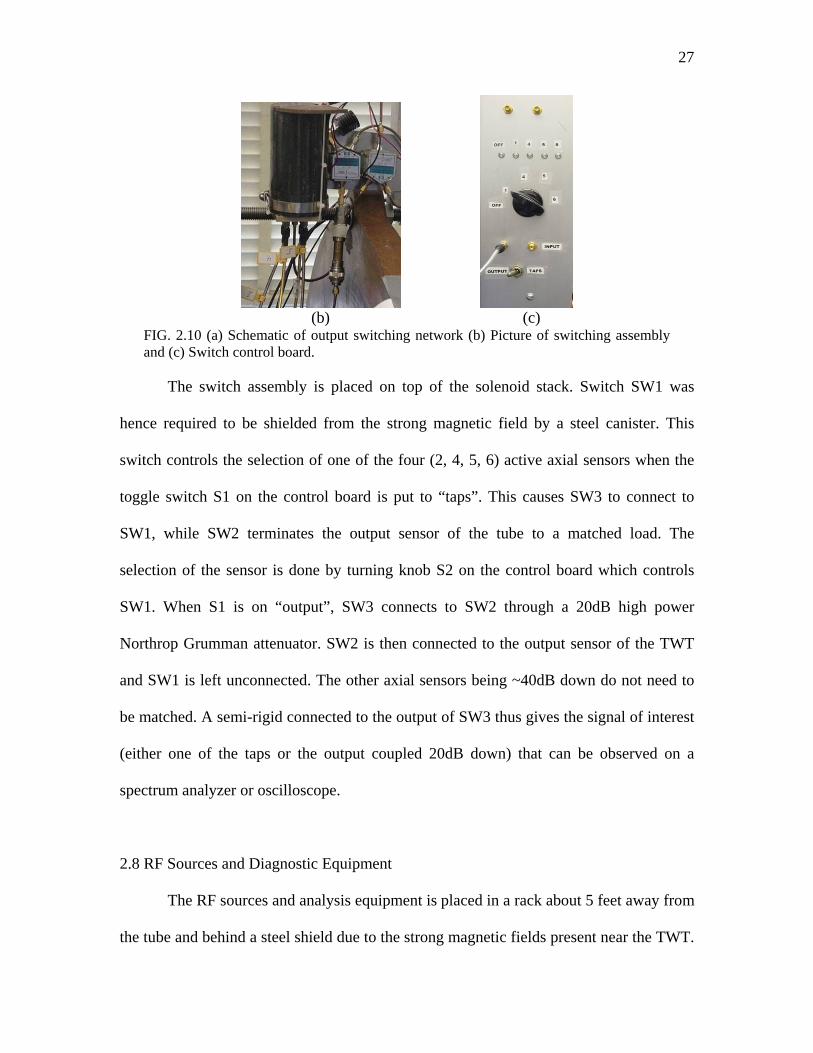
monitoring the output signals. Figure 2.10 shows the switching configuration and the
control board.
(a)
--2200ddBB AAttttnn..
27
(b) (c)
FIG. 2.10 (a) Schematic of output switching network (b) Picture of switching assembly and (c) Switch control board.
The switch assembly is placed on top of the solenoid stack. Switch SW1 was
hence required to be shielded from the strong magnetic field by a steel canister. This
switch controls the selection of one of the four (2, 4, 5, 6) active axial sensors when the
toggle switch S1 on the control board is put to “taps”. This causes SW3 to connect to
SW1, while SW2 terminates the output sensor of the tube to a matched load. The
selection of the sensor is done by turning knob S2 on the control board which controls
SW1. When S1 is on “output”, SW3 connects to SW2 through a 20dB high power
Northrop Grumman attenuator. SW2 is then connected to the output sensor of the TWT
and SW1 is left unconnected. The other axial sensors being ~40dB down do not need to
be matched. A semi-rigid connected to the output of SW3 thus gives the signal of interest
(either one of the taps or the output coupled 20dB down) that can be observed on a
spectrum analyzer or oscilloscope.
2.8 RF Sources and Diagnostic Equipment
The RF sources and analysis equipment is placed in a rack about 5 feet away from
the tube and behind a steel shield due to the strong magnetic fields present near the TWT.

28
The rack containing the primary equipment used for experimental measurements on the
XWING is shown below in Fig. 2.11.
FIG. 2.11 Photo of primary laboratory RF diagnostic equipment.
The RF sources include two Agilent 83626B digital frequency synthesizers. These
signal generators can provide a signal ranging from 10 MHz - 20 GHz and up to 25 dBm
output power. These generators can be frequency-locked by sharing a 10MHz reference
signal.5 Thus there is provision for two-tone excitation of the TWT. Additional input
signals can be generated by using frequency doublers and mixers.
RF analysis equipment available includes primarily a power meter, two digital
oscilloscopes and a spectrum analyzer. The HP 437B power meter with an 8482A power
sensor is used for continuous power measurements to measure actual input power,
characterize losses etc. However, to measure accurate spectral distribution of power, a
spectrum analyzer must be used.
5 Frequency-locking does not essentially imply phase-locking. Though the phases from the two frequency-locked generators trace closely, there is a certain phase drift with time.
29
The LeCroy 9354TM digital oscilloscope is a DC - 500 MHz scope with sampling
rate up to 2 Gs/sec. It is used to monitor the cathode voltage pulse as well as cathode and
collector currents, and other low frequency signals.
For higher frequency pulsed measurements, it may be of interest to look at the RF
signal during the steady-state part of the pulse duration only. This requires gating feature
on the analysis equipment. The lab is equipped with a time-gated Agilent 86100A
wideband oscilloscope for time-domain measurements and a time-gated HP 8563EC
spectrum analyzer for frequency-domain measurements. The 86100A oscilloscope has
two plug-in modules with 20 and 50 GHz bandwidth with sample speeds up to 40 Gb/sec.
The HP 8563EC Spectrum analyzer works for 30 Hz – 26.5 GHz signals and can be gated
by an externally applied trigger. The gate delay and gate width can be specified in the
spectrum analyzer, and no external trimming circuit is needed to look at part of a pulse.
Significance of time-gating:
The ability to time-gate the instrument allows data acquisition only during part of
the pulse duration when a valid steady-state signal is present. Sufficient data is acquired
over several hundred pulses to recreate a continuous representation of the waveform. As
seen in Figs. 2.4 and 2.9, the XWING cathode voltage and currents vary slightly over the
duration of the pulse. This variation is significant for this tube as XWING is fairly
sensitive to detuning (difference between beam velocity and cold-circuit phase velocity).
This causes the device response to vary in time, causing variations in the small-signal
gain, saturated gain etc over the pulse duration and making characterization of the tube
difficult. To illustrate the effects of this droop in voltage Fig. 2.12 shows a Lecroy trace

30
of the output power as a function of time for a steady state 4.00 GHz signal at 10 dBm.
The trace was obtained by mixing the XWING output with a 4.02 GHz signal. The output
of the mixer at 20 MHz is proportional to the output power of the tube. Clearly, the
output power and gain vary over the pulse duration.
FIG. 2.12 Output power (trace 4) and hence gain variation over the pulse duration due to voltage droop at 4 GHz.
To address this issue, a gate delay of 300 µs and a gate width of 100 µs is used (as
shown in Fig. 2.9, trace 4) for XWING pulsed measurements to remove ringing effects
and collect data during a relatively constant portion of the voltage pulse. In this region,
based on similar instantaneous measurements, the gain of various frequencies was found
to be relatively constant for frequencies from 1-6 GHz.
Setting Parameters for time-gate measurement on the HP 8563EC Spectrum Analyzer
Time-gated data acquisition on the Spectrum Analyzer requires understanding
some other inter-dependent parameters that need to be set right. These parameters include
resolution bandwidth (RBW), video bandwidth (VBW), span and sweep time. Figure
2.13 shows a Block diagram of the Spectrum analyzer with time-gating.

31
FIG. 2.13 Block diagram of a time-gated spectrum analyzer.
The IF resolution bandwidth filter determines the minimum spacing between two
closely spaced signals that can be resolved on the spectrum analyzer. However, setting
the RBW too narrow may cause the power at a frequency to read lower since the filters
may not be able to charge to the proper value since:
Charge time of the RB filter RBW/1∝
For good time-gated data acquisition, the gate delay should be enough to allow the RB
filter to charge up and hence,
Gate delay > RBW/2
Usually the gate delay is limited by the actual pulse shape and duration and hence a good
rule of thumb is to keep the RBW at the maximum value that still allows the frequencies
of interest to be resolved.
The video bandwidth filter smoothes or averages the signal to reduce noise. To
ensure that a true peak value is obtained before the gate goes off, the video filter must
have a charge time of less than the gate length.
Gate length > RBW/1
∼ DISPLAY LOGIC
MIXER
IF LOG AMPLIFIER
ENVELOPE DETECTOR (IF to VIDEO)
GATE
VIDEO BANDWIDTH FILTER
PEAK/ SAMPLE DETECTOR
LOCAL OSCILLATOR
SCAN GENERATOR
DISPLAY
IF RESOLUTION BANDWIDTH FILTER
RF INPUT ATTENUATOR
RF INPUT
ANALOG/ DIGITAL CONVERTER
32
Again, a good rule of thumb is to keep the VBW maximum and reduce it gradually until a
drop in power level is observed.
The span value setting also controls the obtainable resolution and accuracy of
power level at a particular frequency. If the span is wide, a large number of sample points
are desired to obtain the correct power reading. This implies longer sweep times. If sweep
time is too low, the spectral peaks may be reduced. In any case, the sweep time should be
greater than 601 times the pulse repetition interval to ensure that the gate is on at least
once during each of the 601 digital trace points.
Sweep time > 601 x PRI (pulse repetition interval)
Ideally, the sweep time should be kept high and then reduced until an acceptable drop in
power level is obtained.
To obtain accurate power level readings, the reference level should be kept close
to the level of the input signal. Signals measured much below the reference level have
some inherent error in amplitude reading. Also very low-level signals may be lost in the
noise floor of the spectrum analyzer. Changing reference level changes the input
attenuator causing the low-level signals to be visible. On the other hand, high-level
signals may cause internal spectrum analyzer distortion products to corrupt the readings.
So care must be taken in setting the input attenuator or the signal should be externally
attenuated. Multi-tone input signals that vary widely in amplitude, eg. intermodulation
spectra and fundamental frequencies, present another problem. Accurate amplitude
measurements for this case require that either each frequency be focused in turn and
reference level adjusted, or a delta-marker measurement be used to characterize
intermodulation amplitude as a dBc (dB below carrier) of the fundamental.

33
2.9 Experimental Set-up for Suppression using Signal Injection
This section explains the experimental set-up required for observing suppression
of spectral content at a frequency by an input signal injected along with the fundamental
tones. A block diagram of the set-up is presented in Fig. 2.14 for the case of exciting the
XWING with two fundamental tones (fa, fb) and two injection signals – a harmonic (say
2fb) and a third-order intermodulation signal (say 2fb-fa). This case presents ideas for
investigating all other signal injection schemes.
FIG. 2.14 Experimental set-up for XWING linearization using simultaneous injection of second-harmonic and 3IM along with the two fundamental drive tones. (For second-harmonic injection, only the second-harmonic is combined with the fundamentals at the high-power combiner while the 3IM from the mixer is terminated with a matched impedance, and vice-versa for 3IM injection only.)
x2
f1 1.90 GHz f2 1.95 GHz
Solid State Amplifiers
High-powerCombiner
Phase shifter
Variable Attenuators
Semi RigidCoax
TWT
Gated Spectrum Analyzer
X
Mixer
Frequency doubler
LO RF
IF

34
The two fundamental signals fa at 1.90 and fb at 1.95 GHz are generated using the
two Agilent 83623B signal generators. These two generators are frequency-locked by
sharing a 10MHz reference to avoid any frequency jitter. The harmonic signal 2fb at 3.90
GHz is generated from the fundamental f2 using a frequency doubler.6 The 3IM 2fb-fa at
2.00 GHz is generated by mixing the harmonic 2fb and fundamental fa.
Power levels on the Agilent generators are determined by the input power
specifications to the frequency doubler and the mixer. Thus attenuators are needed to
control the fundamentals’ power level input to the TWT. The harmonic and 3IM are
adjusted in amplitude by a series of two attenuators – a coarse 1 dB step attenuator
followed by a multi-turn dial fine attenuator. The phase is adjusted using two Narda 1-5
GHz phase shifters with 0.2°/GHz resolution. Since varying the attenuators also causes
the phase shift through them to change slightly, achieving a precise amplitude and phase
shift requires a careful iteration of both elements. Also as doublers and mixers are
nonlinear devices, the output signal from these devices are verified for presence of
undesired frequencies. This may require adjusting the input power level to these devices.
This set-up is placed away from the strong magnetic fields surrounding the tube.
These four signals are then taken close to the TWT input using semi-rigid coax. Losses in
the cables and components weaken the signal strength and thus these need to be boosted
using solid-state preamplifiers. However, care is taken to operate the pre-amplifiers in
back-off to reduce any nonlinear products in the preamps’ outputs. Four solid-state
preamplifiers are available in the lab. Two of these are identical HD Comm. 19340
amplifiers over 0.8-2.5 GHz with 15 W of max saturated output power, 42 dB gain that
6 Earlier a separate frequency generator was used to obtain the second harmonic, however phase drifts between the fundamental and harmonic generators resulted in lower suppression [28].
35
are used for amplifying the fundamental signals, and are sufficient to drive the XWING
all the way to saturation. A ZHL-42W Minicircuits 10 MHz - 4.2 GHz, 30 dB gain
amplifer is used for amplifying the harmonic, while a ZHL-1042J Minicircuits 10 MHz -
4.2 GHz, 25 dB gain amplifier is used for the 3IM. These amplifiers were tested to have
harmonic and spurious frequency content < 20 dB below the frequency being amplified.
These four signals are then combined using a high-power combiner and fed to the
XWING input. Since the two fundamentals will be at much higher power levels than the
amount of injected harmonic and 3IM needed, isolators may need to be used to prevent
any fundamental signals from feeding back into the harmonic and 3IM paths and
disturbing the performance of other components. Due to dispersion effects in the coax
and cables (Appendix F) and insertion losses of the various components, the input
spectrum to the TWT should be verified and adjusted by observing the combiner’s output
on the spectrum analyzer using a 2 ft. flexible cable similar to the one that feeds to the
XWING input.
The output signal from the tube is chosen by the switching assembly. A coax
cable conveys the signal from the switch assembly on top of the solenoids to the switch
control board located on top of the equipment rack. The output signal is now monitored
on a spectrum analyzer. The time-gating signal for the spectrum analyzer is obtained
from the TTL pulser box connected to the NorthStar pulse generator. Loss in the output
semi-rigid and switching assembly was also characterized (Appendix G) and accounted
for either manually or feeding as an amplitude correction table in the spectrum analyzer.
An attenuator may be needed at the input to the spectrum analyzer to prevent generation
of nonlinear products from the spectrum analyzer’s internal mixer that may corrupt the
36
measurements. Also, the maximum input power to the spectrum analyzer is limited at 30
dBm.
2.10 Discussion of Experimental Errors
Experimental errors arise from a variety of sources including day-to-day
variations in operating conditions, built-in error of analysis equipment, fluctuations in
attenuation or phase at GHz frequencies with slight movement of cables/tightening of
screws and variation of quantities like magnetic field and preamplifier gain due to slight
heating while running for long times. Characterizing and understanding these
experimental errors is crucial to the extraction of meaningful data and precise
measurements.
There are two kinds of experimental errors that need to be mentioned. One set is
due to day-to-day variations in cathode conditioning and operating conditions such as
temperature and pressure that reflect as changes in gain. These errors are determined to
be ±1 dB for the XWING tube. However, these variations affect all frequencies equally
and the relative levels are found to be accurate within the second set of errors. The
second set includes shot-to-shot variation in power levels, inaccuracies of spectrum
analyzer in characterizing low level signals, heating effects, variation in attenuation and
phase with the tightening of adjustment screws, cable movement and small phase drifts in
the output of the synthesizers. Attempts are made to keep these errors small e.g.
preventing heating by cooling techniques, keeping the input signals’ power level close to
the reference in the spectrum analyzer and frequency locking the synthesizers).
Nevertheless, some errors such as shot-to-shot variation, spectrum analyzer inaccuracies

37
in reading correct power levels even when reference level is low enough, and inability to
precisely tune the correct amplitude and phase combination using manual phase-shifters
and attenuators cannot be avoided. The power measurements shown in Chapters 3 and 4
were taken by focusing on a single frequency and keeping the reference level close to the
power level being measured. The frequency span was kept at 50 MHz to get a fine
resolution of ~ 0.1 MHz/point (= 50 MHz/601 pts per sweep). With a cathode pulse
repetition rate of 5 Hz, at least one shot per frequency point requires 0.2 secs/point or 120
secs/sweep. Thus, the sweep time was kept at 150 secs to ensure at least one cathode
voltage pulse occurring per frequency point. While it is desirable to get an average power
measurement over more than a single shot, excessive sweep times are required. Thus it is
crucial to characterize the error due to shot-to-shot variations.
Characterization of these unavoidable errors shows that typical shot-to-shot (i.e.
over several cathode voltage pulses) variation in power level is typically ±0.2 dB for high
power levels and increases (up to ±0.7 dB) for power levels close to the noise floor. For
the cases considered in this thesis, the fundamental power levels are typically within ±0.2
dB, second-harmonics and 3IMs are within ±0.3 dB and 5IMs are within ±0.5 dB. With
injection, the power levels at the suppressed frequencies are very small and drifts in
phase and amplitude also contribute to the error resulting in typically ±1 dB error in the
amount of suppression obtained. In most cases, these errors are negligible compared to
the quantities of interest. However, we mention the error bars for each case. The error
bars quoted are of the second set when we are comparing quantities measured on same
day to reveal the relative pattern, since the day-to-day variations affect all frequencies
equally.
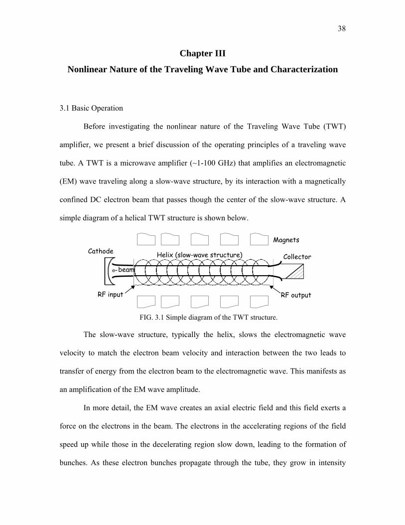
38
Chapter III
Nonlinear Nature of the Traveling Wave Tube and Characterization
3.1 Basic Operation
Before investigating the nonlinear nature of the Traveling Wave Tube (TWT)
amplifier, we present a brief discussion of the operating principles of a traveling wave
tube. A TWT is a microwave amplifier (~1-100 GHz) that amplifies an electromagnetic
(EM) wave traveling along a slow-wave structure, by its interaction with a magnetically
confined DC electron beam that passes though the center of the slow-wave structure. A
simple diagram of a helical TWT structure is shown below.
FIG. 3.1 Simple diagram of the TWT structure.
The slow-wave structure, typically the helix, slows the electromagnetic wave
velocity to match the electron beam velocity and interaction between the two leads to
transfer of energy from the electron beam to the electromagnetic wave. This manifests as
an amplification of the EM wave amplitude.
In more detail, the EM wave creates an axial electric field and this field exerts a
force on the electrons in the beam. The electrons in the accelerating regions of the field
speed up while those in the decelerating region slow down, leading to the formation of
bunches. As these electron bunches propagate through the tube, they grow in intensity
Collector Helix (slow-wave structure)
RF input RF output
e- beam
Cathode Magnets

39
and start losing energy to the EM wave leading to exponential growth of the wave. When
the electrons have lost sufficient energy, they slow down and slip into the decelerating
regions now taking back energy from the wave and leading to reduction in wave
amplitude. This phenomenon is called saturation. The amplifier provides maximum
amplification when the TWT amplifier output is taken just before onset of saturation.
Figure 3.2 illustrates the formation of electron bunches and the growth of the EM wave
through saturation.
FIG. 3.2 Formation of electron bunches (color shows the intensity of the bunches) and growth of EM wave.
Only a brief overview of TWT operation is presented here. A more complete
discussion of the TWT theory can be found in several books eg. by Pierce [22] and
Gilmour [14].
3.2 Nonlinear Nature and Characterization
The nonlinearity of a system manifests as amplitude, phase and spectral distortion
in the output signal. As discussed in Section 1.1.1, for single-tone inputs nonlinearity
leads to generation of harmonics, and for multi-tone inputs it leads to both harmonics and
Bunch formation Exponential gain Saturation Electron bunches
Wave Amplitude

40
intermodulation distortion products. Apart from frequency-domain spectral distortion, the
more apparent time-domain distortions are in the amplitude and phase of the output
signal. Hence, traditionally an amplifier’s nonlinearity has been specified in terms of its
amplitude and phase distortion transfer functions.
3.2.1 AM/AM and AM/PM characterization
If the input to a nonlinear amplifier is a single-tone given as
(3.1)
then the output signal can be written as
(3.2)
where A[r(t)] is the amplitude distortion and ∆Ф[r(t)] is the phase distortion. Therefore,
nonlinear amplifiers are generally characterized in terms of an amplitude distortion
(AM/AM) curve and a phase distortion (AM/PM) curve based on the envelope of the
input signal as shown below.
FIG. 3.3 Nonlinear characterization of an amplifier using (a) Amplitude distortion A[r(t)] curve or AM/AM curve (b) Phase distortion ∆Ф[r(t)] curve or AM/PM curve.
The AM/AM curve depicts that the output power is a linear function of the input
power for small drive levels. As the amplifier is driven harder (more input power), the
Pin Pin
∆Φ
A[r(t)] ∆Φ[r(t)]
Pout
( ) [ ] [ ][ ])(cos)( trttrAtV cout ∆Φ+= ω
( ) ( )ttrtV cin ωsco)(=
(a) (b)

41
function becomes nonlinear and the device goes to saturation. For a TWT saturation kicks
in as the electrons slow down and slip in phase with respect to the electromagnetic wave,
taking back energy from the wave. Thus with over-drive, the output power reduces for a
TWT amplifier. (This is unlike solid-state amplifiers where the output power remains
constant after saturation.)
The AM/PM curve represents the phase shift of the output signal wrt to the input
signal. While the phase difference remains constant for lower drives, phase of the output
signal distorts as the input power is increased. This phase deviation is attributed
traditionally to the average slowing down of electrons as the tube is driven harder [14].
More recently, it has been shown [29, 30] that the generation of second-harmonic and not
the DC slowing down of the electrons is the primary cause of phase distortion, as
explained in section 3.2.2. It should be noted that the phase distortion occurs much before
the onset of nonlinearity due to the AM/AM curve. Hence, phase distortion is primarily
responsible for nonlinearity of the TWT amplifier.
The AM/AM and AM/PM curves model the nonlinear amplifier’s transfer
function at a particular frequency. Saleh [24] provided a similar model for TWTs where
he proposed the following two-parameter formulas:
21)(
rrrAa
a
βα+
= and 2
2
1)(
rr
rφ
φ
βα+
=∆Φ (3.3)
These curves specify the amplifier’s output as a function of the envelope of the input
signal, rather than its instantaneous value. While such a single-frequency transfer curve
characterization is valid for most solid-state amplifiers, it does not explain the broadband
TWT nonlinearities completely. Dispersion or memory-effects in the TWTs cause the
shape of the AM/AM and AM/PM curves to change with frequency. While this can be

42
taken into account by making the parameters αa, βa, αφ and βφ frequency-dependent as
suggested in [24], the resulting analysis for multi-tone excitation is not difficult and
incorrect. However, if the multiple input tones are closely spaced, the same AM/AM and
AM/PM transfer curves can be used to derive the output signal content. Assuming r to be
time-varying, a two-tone input can be written as
(3.4)
( )( ) ( )( )[ ] coscos2a tt mcmc ωωωω −++=
As long as cm ωω << , the output signal can be written as
(3.5)
The AM/AM and AM/PM curves in terms of voltage actually look like the following:
(a) (b)
FIG. 3.4 Voltage transfer curves (a) AM/AM (odd-function) and (b) AM/PM (even function).
Hence, A(r) and ∆Ф(r) are odd-order and even-order functions respectively. Using this
condition, we see that the output voltage contains all intermodulation frequencies spaced
2ωm apart. Considering only AM/AM distortion,
(3.6)
which contains terms at frequencies ωc ± (2k+1)ωm. Similarly, considering AM/AM to be
linear it can be seen the phase distortion AM/PM produces intermodulation products in a
similar fashion.
A(r)
r r
∆Φ(r)
( ) ( ) ( ) ( )ttattrtV cmcin ωωω coscoscos)( ==
( ) ( )[ ] ( )[ ][ ]tattaAtV mcmout ωωω coscoscos ∆Φ+=
( ) ( ) [ ]00
1212 coscos φωω += ∑=
++ ttatV c
M
km
kkout

43
(3.7)
Thus, AM/AM and AM/PM curves can be used to predict intermodulation
products around the fundamentals for closely spaced tones. However, as the spacing
between the drive tones increases, the AM/AM and AM/PM curves do not predict the
correct values for power at the intermodulation frequencies. Section 5.3 of Ref [29]
presents a good comparison of the predicted power for varying tone-separation using
these curves and the MUSE model. The latter is a TWT model based on the physics of
the device and is described in the next section.
Further, it should be noted that the AM/AM and AM/PM curves provide
information about frequencies lying around the fundamentals but do not predict the
generation of harmonics, which are essential for describing the nonlinearity of a TWT
amplifier. As shown in the next section, second harmonic frequency influences the phase
distortion at the fundamental frequency through an intermodulation process.
These curves also fail to justify the presence of harmonics in the so-called linear
region of these curves for a TWT. Experimental measurements presented in Section 3.3
show that harmonics are present in the output spectrum even for drive levels much below
saturation. This phenomenon can be explained on the basis of the device physics.
Simulation done using IBC, a 1D time-domain TWT code [21], show that even while the
circuit voltage grows exponentially i.e. linearly on a dB scale, the e- beam bunching is
clearly non-sinusoidal showing the presence of harmonics in the output voltage prior to
saturation.
( ) ( ) ⎥⎦
⎤⎢⎣
⎡+= ∑
=
N
km
kkcmout tattatV
1
22 )(coscoscos ωωω

44
Circ
uit
volta
gez=0 z=LAxial position
Circ
uit
volta
gez=0 z=LAxial position
Axial position z=Lz=0
Beam
cur
rent
Axial position z=Lz=0
Beam
cur
rent
FIG. 3.5 Circuit voltage and electron beam current showing presence of harmonic content in the beam prior to voltage saturation. (Simulations done using IBC code [21]).
Thus, while AM/AM and AM/PM curves characterize some aspects of the
nonlinear behavior, they do not provide a complete view of the nonlinear distortion
mechanism in a traveling wave tube.
3.2.2 MUSE (MUlti-frequency Spectral Eulerian) model
The inability of the AM/AM and AM/PM curves to predict the presence of
harmonic distortion in the TWT output spectra necessitates the use of a model based on
the basic equations governing the device physics. A spectral domain TWT model is
preferred since it gives a better understanding of the spectral distortions characterizing
the TWT nonlinearity. MUSE [29, 32] is a 1-D nonlinear frequency-domain TWT model,
based on a spectral analysis of the transmission line equations used to represent the slow-
wave circuit and Eulerian electron beam equations, is well-suited for this purpose. S-
MUSE, a simplified analytically solvable version of the MUSE model obtained by
neglecting certain nonlinearities [29], is used in this thesis to provide the physical

45
mechanism responsible for various experimental observations. However, for comparison
with experimental data a similar Lagrangian “large-signal code”, LAgrangian TWT
Equations or LATTE, based on the same starting equations is used. This model is more
appropriate for this comparison, so that experimental details such as an attenuating sever
between two sections of the helix can be accounted for. Also LATTE can predict
saturation effects while MUSE and S-MUSE do not include electron overtaking and
hence cannot predict saturation. However, these models agree well before saturation. See
Ref. [29, 32] for details of these models.
MUSE (as well as S-MUSE) is a system of ordinary differential equations for the
spatially dependent complex Fourier coefficients of the five quantities in the TWT
description: transmission line voltage ( )zV~ , transmission line current ( )zI~ , space
charge electric field ( )zE~ , electron beam velocity ( )zv~ , and electron beam charge
density ( )zρ~ , where is a frequency index and z is the axial distance. The model is
steady-state and assumes that all frequencies are integer-multiples of a base frequency ω0.
Each frequency fl (actually flω0)1 is viewed as a nonlinear distortion product of order K
for input frequencies f1, f2, …, fp:
fl = r1f1 + r2f2 + … + rpfp (3.8)
where rjs are integers (possibly zero) and K = |r1| + |r2| + … + |rp|.
This structure represents input quantities if all rjs are zero except one which is
equal to 1 and hence is a first-order product. Harmonics are represented by all rjs being
1 A multiplying factor of ω0 should be assumed for this model even if not explicitly stated. A frequency of fk is actually a misnomer and refers to frequency of flω0.
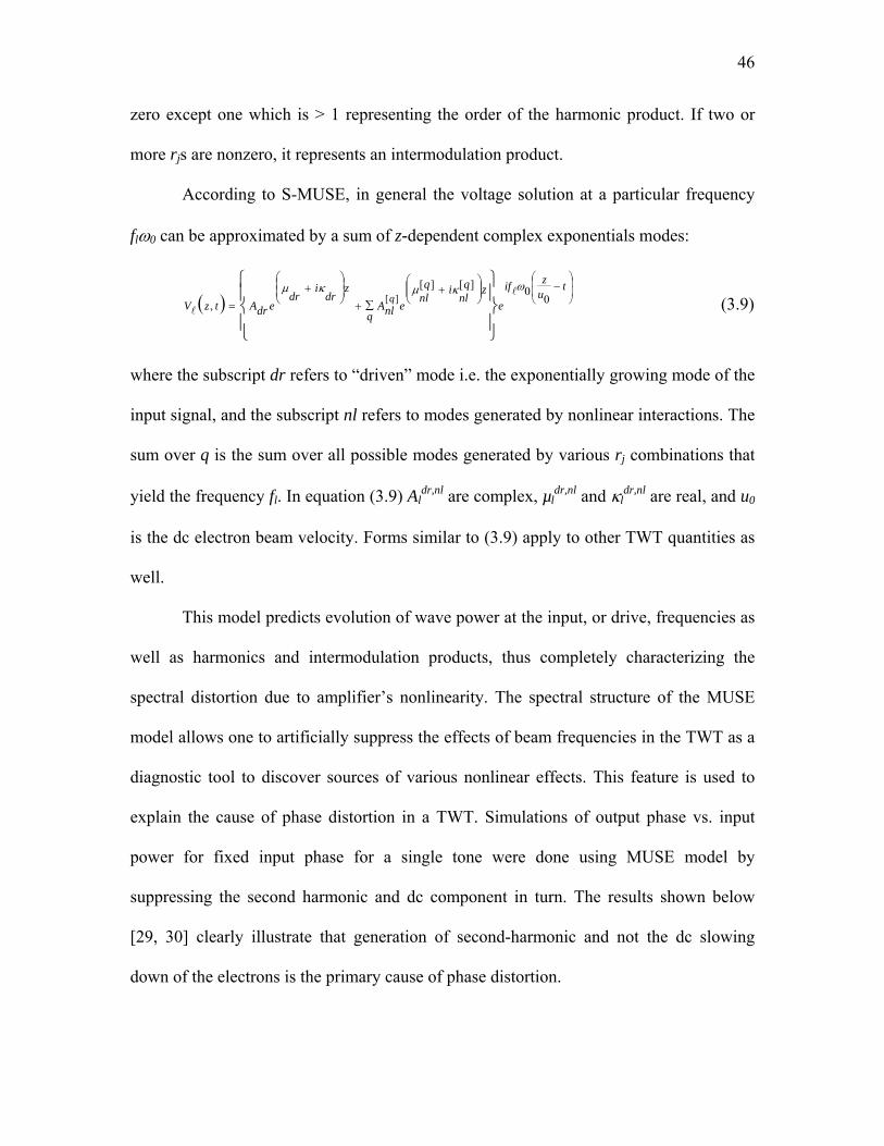
46
zero except one which is > 1 representing the order of the harmonic product. If two or
more rjs are nonzero, it represents an intermodulation product.
According to S-MUSE, in general the voltage solution at a particular frequency
flω0 can be approximated by a sum of z-dependent complex exponentials modes:
( )⎟⎟
⎠
⎞
⎜⎜
⎝
⎛−
∑⎟⎟⎠
⎞⎜⎜⎝
⎛+
+⎟⎟⎠
⎞⎜⎜⎝
⎛+
=
⎪⎭
⎪⎬
⎫
⎪⎩
⎪⎨
⎧ tuzif
eq
zqnl
iqnl
enlAz
dri
dredrAtzV
q 00][][
,][
ωκµκµ (3.9)
where the subscript dr refers to “driven” mode i.e. the exponentially growing mode of the
input signal, and the subscript nl refers to modes generated by nonlinear interactions. The
sum over q is the sum over all possible modes generated by various rj combinations that
yield the frequency fl. In equation (3.9) Aldr,nl are complex, µl
dr,nl and κldr,nl are real, and u0
is the dc electron beam velocity. Forms similar to (3.9) apply to other TWT quantities as
well.
This model predicts evolution of wave power at the input, or drive, frequencies as
well as harmonics and intermodulation products, thus completely characterizing the
spectral distortion due to amplifier’s nonlinearity. The spectral structure of the MUSE
model allows one to artificially suppress the effects of beam frequencies in the TWT as a
diagnostic tool to discover sources of various nonlinear effects. This feature is used to
explain the cause of phase distortion in a TWT. Simulations of output phase vs. input
power for fixed input phase for a single tone were done using MUSE model by
suppressing the second harmonic and dc component in turn. The results shown below
[29, 30] clearly illustrate that generation of second-harmonic and not the dc slowing
down of the electrons is the primary cause of phase distortion.
47
FIG. 3.6 MUSE simulation from Ref. [29, 30] showing that harmonic generation, and not dc reduction of beam velocity, is the primary cause of phase distortion in TWTs.
In the case shown above, dc slowing down can account for only ~13% of the
observed phase distortion (1.3° out of 10°). Fig. 3.7 shows the phase evolution for two
different power levels. Spatial evolution of the beam velocity for these power levels also
shows that the dc level changes very slightly while the harmonic content is significant.
(a) (b)
FIG. 3.7 (a) Phase evolution of the wave for two different input power levels, and (b) Spatial evolution of the beam velocity for the same power levels. (from Ref. [29,30])
As seen in Fig. 3.7(a), phase distortion occurs due to a change in the wavelength,
which is due to change in the phase velocity with drive power for the same frequency.
This change in phase velocity can be explained by the MUSE model if we consider all the

48
modes contributing to that frequency. Apart from the driven mode at the fundamental
frequency, there exists a nonlinear third-order mode due to beating of nonlinearly
generated second-harmonic with the fundamental and similarly, a fifth-order mode due to
beating of the third-harmonic with the second-harmonic and so on.
(3.10)
All these modes have different phase velocities and wavelengths, leading to a
change in net phase velocity for the fundamental frequency. This is the primary cause of
phase distortion. Since harmonics are present in the output spectrum much before
saturation, the phase distortion occurs much earlier than amplitude distortion.
3.3 Experimental characterization of the XWING nonlinearities
It is important to understand the nonlinear behavior of the tube before
linearization schemes can be explored. Experimental measurements were conducted to
characterize the frequency dependent behavior and the nonlinearities of the customized
research TWT – the XWING.
Unless otherwise stated most of the experimental data (power readings) have been
measured using the HP 8563EC gated spectrum analyzer. The spectrum analyzer allows
the measurement of the spectral distribution of power by isolating the frequency of
interest from other frequencies. On the other hand, devices like the power meter and
diode detector give a time-averaged power across the device bandwidth. Time-gating
enables measurement of pulsed output power as explained in Chapter 2. Also, care was
taken to keep the Ref level on the spectrum analyzer constant by varying an external
...]5[]3[ ≠≠≠ nlnldr κκκ
( ) ( ) ( ) ( ) ...,]5[]5[]3[]3[ ]5[]3[
1 +++= +++ zinl
zinl
zidr
nlnlnlnldrdr eAeAeAtzV κµκµκµ

49
precision attenuator at the input to the spectrum analyzer. This prevents any distortion
products internal to the spectrum analyzer from corrupting the results due to differential
driving of the input mixer.
3.3.1 Gain vs. frequency
The output power and gain vs. frequency were measured for three different input
powers -10 dBm, 0 dBm and 15 dBm for frequencies from 1-7 GHz. The power
measurements were done on the spectrum analyzer and frequency dependent cable losses
were accounted for. Figure 3.8 shows the results. Measurement error is estimated to be
±1dB, which is primarily attributed to day-to-day variations in cathode conditioning and
operating conditions as discussed in Section 2.10.
-5
0
5
10
15
20
25
30
35
1 2 3 4 5 6 7
Frequency (GHz)
Gai
n (d
B)
-10 dBm0 dBm15 dBm
FIG. 3.8 Characterization of XWING Gain vs. frequency for three input powers: -10, 0 and 15 dBm.
50
Clearly the XWING TWT amplifier produces gain for frequencies even beyond
the specified 2-6 GHz range. The gain of the tube peaks at ~30 dB for a frequency
slightly less than 4 GHz. Thus the tube is broadband, a little less than 2 octaves wide, and
offers a large bandwidth for investigating nonlinear distortions such as harmonics.
Instantaneous (time-domain) gain measurements similar to Fig. 2.12 were also
taken by characterizing the mixer, to verify the accuracy of the data. Both set of readings
agreed within 1dB.
Simulations were done using LATTE to compare the model against experimental
data. Some simulation parameters were required to be adjusted to obtain a good fit and
are discussed in Chapter 4 of Ref. [7]. Figure 3.9 shows the comparison for 0dBm input
power. Though the simulation does not always lie within the error bars (±1 dB), it a
reasonable fit given that the model is 1D and does not include 3D effects present in the
high-space charge XWING TWT. The discrepancy at 6 GHz can be understood by
looking at the drive curves discussed in the next section.
-5
0
5
10
15
20
25
30
35
1 2 3 4 5 6 7
Frequency (GHz)
Gai
n (d
B)
0 dBm Simulation0 dBm Experiment
FIG. 3.9 Small-signal gain comparison of the XWING TWT.
51
3.3.2 Single-tone drive curve characterization
Drive curves were obtained for 1-7 GHz within the gain bandwidth of the
XWING TWT. The tube was driven with a single tone and input power was swept from -
10 dBm to ~ +30 dBm, depending on the maximum power available from the pre-
amplifiers. The corresponding output power was recorded on a spectrum analyzer to yield
drive curves similar to an AM/AM characterization at each frequency.2
-30
-20
-10
0
10
20
30
40
50
-20 -15 -10 -5 0 5 10 15 20 25 30Pin (dBm)
Pout
(dB
m)
1 GHz 2 GHz3 GHz 4 GHz5 GHz 6 GHz7 GHz
FIG. 3.10 Single-tone drive curve (AM/AM) characterization of the XWING TWT. (Error bars are characterized to be ±1 dB (Section 2.10) and are too small to be visible on the graph)
Figure 3.10 shows that XWING is capable of providing maximum output power >
48 dBm or ~ 65 W at 4 GHz. All frequencies show a linear Gain upto input powers of ~ 2 An AM/PM curve characterization was not done due to experimental difficulties of extracting precise phase information from pulsed measurements at high frequency. Pulsed measurements on the high frequency Agilent scope require time-gating. Droop on the cathode voltage during the gating period distorts the waveform on the oscilloscope, rendering phase information useless. However, acceptable amplitude information can still be obtained on a gated spectrum analyzer or by downconverting the frequency. Homodyning is one possibility that can be explored to measure phase, though it requires precise characterization of the mixer characteristics.

52
15 dBm, after which gain compression starts as evidenced by the decrease in slopes.
While the onset of saturation depends on the frequency, the tube is in saturation for input
power > 25 dBm. A sudden decrease in output power is noticeable for frequencies 5, 6
and 7 GHz between 15 – 25 dBm input power. The exact reason for this behavior is not
clear yet, but could be attributed to a resonance in the interaction region or destructive
wave reflection. The behavior of the tube at these frequencies is not very clear and may
explain the difference in simulation and experimental gain observed in Fig. 3.9.
However the curves in Fig. 3.10 only represent the linear growth rate at each
frequency. As explained in the previous section, the growth rate exhibited by a frequency
is different depending on whether it is a driven (or input) mode or is nonlinearly
generated by a kth order interaction. In general, a set of growth rates as shown above
measured with the frequency of interest as a fundamental input (driven mode),
characterize the so-called ‘linear’ growth rate at that frequency. If the frequency of
interest is a second-order product, it has a growth rate approximately twice that of the
linear growth rate for that frequency [29, 33]. In fact for a two-tone drive case, the
growth rate at a frequency mfa±nfb is given as m times the linear growth rate of fa plus n
times the linear growth rate of fb:
]1[]1[][baba ff
nmnfmf nm µµµ +=+
± (3.11)
Experimental measurements were taken to verify this concept. The power at
second-harmonic, 4 GHz was recorded while driving the XWING with a fundamental
input at 2 GHz. Fig 3.11 shows the output powers for both the fundamental and the
second harmonic. The 4 GHz curve for 2 GHz drive is also compared to the drive curve
obtained by driving the tube at 4 GHz.

53
-25
-10
5
20
35
50
-10 -5 0 5 10 15 20 25 30
Pin TWT (dBm)
Pout
TW
T (d
Bm
)
4 GHz2 GHz4 GHz (for 2 GHz input)
FIG. 3.11 Drive curves for 4 GHz as input and 4 GHz as second-harmonic with 2 GHz drive. The curves show that same frequency (4 GHz) has different growth rates as a second-order product and as a driven term. (Error bars: ±1 dB, refer Sec. 2.10)
Clearly, the growth rate at 4 GHz harmonic while driving at 2 GHz is greater than
the linear growth rate at 4 GHz. Also since the 4 GHz harmonic is a second-order
product, its growth rate in the linear region before saturation is approximately twice the
linear growth rate of the 4 GHz drive.
3.3.3 Two-tone drive curve characterization
A single tone characterization of the tube gives an idea of the dispersive nature of
the tube and its frequency-dependent gain. However, a single-drive characterization does
not present a complete picture of the device’s nonlinear behavior for multi-carrier
operation. To gain a better understanding of the XWING nonlinearities, a two-tone drive
curve characterization was carried out. The two drive frequencies were chosen near 2
GHz with a 50 MHz spacing in one case and 500 MHz in another.

54
50 MHz spacing:
In this case, the two drive tones were chosen to be 1.95 and 2.00 GHz. Drive
curves at the two frequencies were obtained for simultaneous injection of the two, by
resolving the tones on the spectrum analyzer. Figure 3.12 presents the results. The figure
also shows a single-tone 2.00 GHz curve for comparison.
14.0
18.0
22.0
26.0
30.0
34.0
38.0
42.0
46.0
-7.0 -2.0 3.0 8.0 13.0 18.0 23.0 28.0 33.0
Pin (dBm)
Pout
(dB
m)
1.95 GHz (two-tone)
2.00 GHz (two-tone)
2.00 GHz (single-tone)
(a)
4.0
6.0
8.0
10.0
12.0
14.0
16.0
18.0
20.0
22.0
-7.0 -2.0 3.0 8.0 13.0 18.0 23.0 28.0 33.0
Pin (dBm)
Gai
n (d
B)
1.95 GHz (two-tone)
2.00 GHz (two-tone)
2.00 GHz (single-tone)
(b)
FIG. 3.12 Two-tone drive-curve characterization of (a) Output power vs. input power (b) Gain vs. input power for 50 MHz spacing between the tones (1.95 GHz and 2.00 GHz). (Error bars: ±0.2 dB (Section 2.10) and are too small to be visible on the graphs).

55
It can be seen that the 2.00 GHz drive curve with single-tone is quite different
from the 2.00 GHz drive curve with two-tone drive. The curves agree for low input
powers but as the tube is driven harder, the presence of another tone results in
intermodulation distortion. The spectrum is now rich in spurious frequencies that rob
power from the fundamentals causing early onset of saturation. In fact, it is not surprising
that for two-tone case the input power/tone required to saturate the tube is ~ 3 dB less (ie
half) than that for single-tone.
In fact, a curve with the total power at two fundamentals vs. total input power,
shown in Figure 3.13 is pretty close to the single-tone drive curve. It is speculated that
curves accounting for total power in the two cases (fundamentals + harmonics +
intermods for two-tone and fundamentals + harmonics for the single tone) will be almost
identical.
14.0
18.0
22.0
26.0
30.0
34.0
38.0
42.0
46.0
-7.0 -2.0 3.0 8.0 13.0 18.0 23.0 28.0 33.0
Pin (dBm)
Pout
(dB
m)
2.00 GHz (single-tone)
1.95 + 2.00 GHz (two-tone)
FIG. 3.13 Comparison of drive curves for single-tone input at 2.00 GHz and total power in the two fundamentals for a two-tone input at 1.95 and 2.00 GHz. (Error bars are estimated to be ±0.2 dB (Section 2.10) and are too small to be visible on the graphs).
56
500 MHz spacing:
In this case, the two drive tones were chosen to be 2.00 and 2.50 GHz.
Experimental results are shown in Fig. 3.14 for two-tone drive as well as for single-tone
drive at these frequencies separately.
14.0
19.0
24.0
29.0
34.0
39.0
44.0
49.0
-7.0 -2.0 3.0 8.0 13.0 18.0 23.0 28.0 33.0
Pin (dBm)
Pout
(dB
m)
2.50 GHz (two-tone)
2.00 GHz (two-tone)
2.50 GHz (single tone)
2.00 GHz (single tone)
(a)
4.00
9.00
14.00
19.00
24.00
29.00
-7.0 -2.0 3.0 8.0 13.0 18.0 23.0 28.0 33.0Pin (dBm)
Gai
n (d
B)
2.50 GHz (two-tone)
2.00 GHz (two-tone)
2.50 GHz (single-tone)
2.00 GHz (single tone)
(b)
FIG. 3.14 Two-tone drive-curve characterization of (a) Output power vs. input power (b) Gain vs. input power for 500 MHz spacing between the tones (2.00 GHz and 2.50 GHz). (Error bars: ±0.2 dB (Section 2.10) are too small to be visible on the graphs).
57
Thus, multi-carrier operation causes saturation, and hence nonlinear distortions, to
occur much earlier. This requires that the tube be operated more backed-off for linear
operation, thus limiting the power efficiency of the device. The closer the spacing of the
two tones, the higher is the interaction and stronger intermods are produced. Thus it is
expected that closer carrier separation causes earlier saturation. A comparison of the 50
MHz separation case with the 500 MHz separation is shown in Fig. 3.15. (In our choice
of frequencies, this difference is not very conspicuous since 2.5 GHz, the 500 MHz
separation carrier has larger gain than the 1.95 GHz carrier for 50 MHz separation case.)
This necessitates the need for linearization even more since effective frequency-space
utilization requires the carriers to be packed as close as possible.
14.0
18.0
22.0
26.0
30.0
34.0
38.0
42.0
-7.0 -2.0 3.0 8.0 13.0 18.0 23.0 28.0 33.0
Pin (dBm)
Pout
(dB
m)
2.00 GHz (two-tone 50 MHz spacing)
2.00 GHz (two-tone 500 MHz spacing)
FIG. 3.15 Comparison of two-tone drive curves with 50 MHz and 500 MHz spacing between the carriers. (Error bars are estimated to be ±0.2 dB (Section 2.10) and are too small to be visible on the graphs).
3.3.4 Small-signal Spatial growth-rate characterization
The unique feature of the XWING, namely the axial sensors, allows measurement
of the spatial growth of frequencies as the wave grows along the tube. This helps to
observe the spatial evolution and growth-rate of various frequencies in the tube.
58
Experiments were done with a single-tone input of 1-7 GHz (the gain-bandwidth
frequencies). The input drive was kept at 0 dBm to ensure small-signal operation. These
measurements are presented in Fig. 3.16 and also serve as a benchmark to evaluate the
LMSuite code [1] for comparison with experimental data. Since no tap coupling loss data
was available for 1 GHz, the loss included in 1 GHz data is actually at 2 GHz.
-25
-15
-5
5
15
25
35
0.0 2.0 4.0 6.0 8.0 10.0 12.0 14.0
axial distance, z (cm)
Pow
er (d
Bm
)
SimulationExperiment
(a) Fundamental at 1 GHz
-25
-15
-5
5
15
25
35
0.0 2.0 4.0 6.0 8.0 10.0 12.0 14.0axial distance, z (cm)
Pow
er (d
Bm
)
SimulationExperiment
(b) Fundamental at 2 GHz
-25
-15
-5
5
15
25
35
0.0 2.0 4.0 6.0 8.0 10.0 12.0 14.0
axial distance, z (cm)
Pow
er (d
Bm
)
SimulationExperiment
(c) Fundamental at 3 GHz

59
-25
-15
-5
5
15
25
35
0.0 2.0 4.0 6.0 8.0 10.0 12.0 14.0axial distance, z (cm)
Pow
er (d
Bm
))
SimulationExperiment
(d) Fundamental at 4 GHz
-25
-15
-5
5
15
25
35
0.0 2.0 4.0 6.0 8.0 10.0 12.0 14.0axial distance, z (cm)
Pow
er (d
Bm
)
SimulationExperiment
(e) Fundamental at 5 GHz
-25
-15
-5
5
15
25
35
0.0 2.0 4.0 6.0 8.0 10.0 12.0 14.0
axial distance, z (cm)
Pow
er (d
Bm
))
SimulationExperiment
(f) Fundamental at 6 GHz
-25
-15
-5
5
15
25
35
0.0 2.0 4.0 6.0 8.0 10.0 12.0 14.0axial distance, z (cm)
Pow
er (d
Bm
)
SimulationExperiment
(g) Fundamental at 7 GHz
FIG. 3.16 Single-tone spatial growth-rate of frequencies in the XWING TWT for small-signal 0 dBm drive.
60
Capturing more than one shot/frequency point with a 5 Hz cathode pulse
repetition rate (0.2 secs/pulse), requires excessive sweep times > 0.2*601freqency points
or 120 secs. However, experimental error bars for shot-to-shot variation are estimated to
be ±0.2-0.7 dB depending on the power level of the signal to be measured (See Sec.
2.10), which are negligible on the scale of the graphs.
It can be seen that the simulations for higher frequencies agree fairly well with the
experimental data, while the lower frequencies deviate specially at sensor 1. Except for 1
GHz which does not follow the trend, this may suggest incorrect modeling of the sever
loss for lower frequencies since sensor 1 lies just after the sever. Accurate tap coupling
measurements are also required at 1 GHz before drawing any conclusions. In this thesis,
we have used the same simulation parameters used for generating Fig. 3.16 since these
yield output gain fairly close to the experimental as seen in Fig. 3.9. However, further
attempt to match the simulation and experimental results was not done and is a topic yet
to be investigated.
The harmonic frequency power was also recorded along with the fundamental
drive for the previous experiment and is shown in Fig. 3.17 only for the lower
frequencies due to unavailability of losses and dispersion data at higher frequencies.
-80
-60
-40
-20
0
20
0.0 2.0 4.0 6.0 8.0 10.0 12.0 14.0axial distance, z (cm)
Pow
er (d
Bm
)
SimulationExperimental
(a) Harmonic at 2 GHz

61
-80
-60
-40
-20
0
20
0.0 2.0 4.0 6.0 8.0 10.0 12.0 14.0axial distance, z (cm)
Pow
er (d
Bm
))
SimulationExperimental
(b) Harmonic at 4 GHz
-80
-60
-40
-20
0
20
0.0 2.0 4.0 6.0 8.0 10.0 12.0 14.0axial distance, z (cm)
Pow
er (d
Bm
)
SimulationExperimental
(c) Harmonic at 6 GHz
FIG. 3.17 Harmonic growth-rate for fundamental drives of (a) 1 GHz, (b) 2 GHz and (c) 3 GHz. Experimental error bars are estimated to be ±0.2-0.7 dB depending on the power level of the signal to be measured as discussed in Sec. 2.10.
The agreement between experimental data and LATTE simulations is again found
to be reasonable except at sensor 1 as for the fundamental. The initial level of harmonic is
as measured at the TWT input and could come from preamplifiers or the signal generator
itself.
3.3.5 Growth of nonlinear products
A characterization of nonlinear distortion products is presented here for the cases
studied in this thesis – a single tone drive at 2 GHz and two-tone drive at 1.90 and 1.95
GHz. These frequencies are used for investigating the various signal injection schemes.
Evolution of distortion products with input power and along the tube axis is measured.

62
For a single tone input at 2 GHz, the harmonic spectral content was found to
increases dramatically as the power increased from 0 dBm to 30 dBm. Since 2 GHz lies
in the lower part of the gain bandwidth, the second harmonic at 4 GHz has higher gain.
The power at 4 GHz becomes comparable to the power at 2 GHz for higher drive levels.
-10 0 15 25 30-30
-20
-10
0
10
20
30
40
50O
utpu
t Pow
er (d
Bm
)
Input Power at 2GHz (dBm)
4 GHz2 GHz
FIG. 3.18 Evolution of harmonic distortion with input power. (Day to day variations exhibit ±1 dB error bars (Sec. 2.10), which are insignificant here).
Spatial evolution of the second-harmonic was also recorded and shows a similar
behavior. Fig. 3.19 shows the power measured at the sensors along the helix in XWING
for 2 GHz, 15 dBm input. Essentially increasing the drive power at the input is equivalent
to moving forward along the axis in terms of nonlinear distortion growth.
input tap 1 tap 4 output-50-40-30-20-10
01020304050
Out
put P
ower
(dB
m)
Input drive at 2GHz (dBm)
4 GHz2 GHz
FIG. 3.19 Spatial evolution of second-harmonic for 2 GHz, 15 dBm drive. (Note that the spacing between the taps shown here is only representative and not the actual distance). (Day to day variations exhibit ±1 dB error bars (Sec. 2.10), which are insignificant here)
63
Measurements were also taken of the relevant nonlinear distortion products for
two-tone drive with 1.90 and 1.95 GHz fundamentals. Two cases, 15 dBm/tone
(beginning of gain compression) and 18 dBm/tone (onset of saturation) are considered as
these power levels were used to test signal injection schemes. Figure 3.20 shows the
results.
IM5- IM3- f1 f2 IM3+ IM5+ 2f1 2f2-20
-10
0
10
20
30
40
Pow
er (d
Bm
)
Spectral frequency
15dBm/tone18dBm/tone
FIG. 3.20 Output spectrum of the XWING for two-tone excitation at 1.90 and 1.95 GHz and drive levels of 15 and 18 dBm/tone. (Experimental error bars are estimated to be ±0.2-0.7 dB depending on the power level of the signal to be measured, refer Sec. 2.10.)
The harmonics are about 15-16 dB below the fundamentals in both cases, while
the third-order intermods are at 27 dBc for 15 dBm/tone and 23 dBc for 18 dBm/tone.
The fifth-order intermods grow much faster by 5-7 dB with increased drive. Thus the
output spectrum gets richer in content as the drive power is increased and higher-order
distortion products become significant.
Spatial evolution of the input tones and nonlinear products generated in the
output spectra of the tube was also measured for the same set of frequencies at 15
dBm/tone or approximately 1 dB gain compression point. The power levels recorded at
the various sensors are shown below.

64
-60
-40
-20
0
20
40
IM5- IM3- f1 f2 IM3+ IM5+ 2f1 2f2Po
wer
(dB
m)
(a) Input
-60
-40
-20
0
20
40
IM5- IM3- f1 f2 IM3+ IM5+ 2f1 2f2
Pow
er (d
Bm
)
(b) Sensor 1
-60
-40
-20
0
20
40
IM5- IM3- f1 f2 IM3+ IM5+ 2f1 2f2
Pow
er (d
Bm
)
(c) Sensor 4
-60
-40
-20
0
20
40
IM5- IM3- f1 f2 IM3+ IM5+ 2f1 2f2
Pow
er (d
Bm
)
(d) Sensor 5

65
-60
-40
-20
0
20
40
IM5- IM3- f1 f2 IM3+ IM5+ 2f1 2f2
Pow
er (d
Bm
)
(e) Sensor 6
-60
-40
-20
0
20
40
IM5- IM3- f1 f2 IM3+ IM5+ 2f1 2f2
Pow
er (d
Bm
)
(f) Output
FIG. 3.21 Spatial evolution of nonlinear distortion components for two-tone excitation at 1.90 and 1.95 GHz with 15 dBm/tone. (Error bars are ±0.2dB for fundamentals, ±0.3dB for 3IMs and second-harmonics and ±0.5dB for 5IMs due to reasons discussed in (Section 2.10) and are insignificant)
The distortion frequencies in the input spectrum arise from the preamplifiers and
are < 30 dBc at the input. A comparison of the two-tone spatial evolution was also done
with LATTE simulations and is shown in Fig 3.22. The simulations and experiment agree
qualitatively, though exact quantitative agreement was not obtained with simple
simulation runs, specially for sensor 1. Part of the reason is the mismatch between the
code and experiment near 2 GHz for small-signal single-tone growth rate sensor 1 as
discussed before.
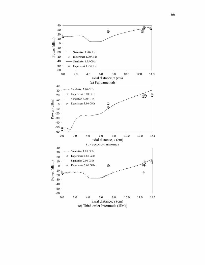
66
-60-50-40-30-20-10
010203040
0.0 2.0 4.0 6.0 8.0 10.0 12.0 14.0axial distance, z (cm)
Pow
er (d
Bm
)Simulation 1.90 GHzExperiment 1.90 GHz
Simulation 1.95 GHzExperiment 1.95 GHz
(a) Fundamentals
-60-50-40-30-20-10
010203040
0.0 2.0 4.0 6.0 8.0 10.0 12.0 14.0axial distance, z (cm)
Pow
er (d
Bm
)
Simulation 3.80 GHzExperiment 3.80 GHz
Simulation 3.90 GHzExperiment 3.90 GHz
(b) Second-harmonics
-60-50-40-30-20-10
010203040
0.0 2.0 4.0 6.0 8.0 10.0 12.0 14.0axial distance, z (cm)
Pow
er (d
Bm
)
Simulation 1.85 GHzExperiment 1.85 GHz
Simulation 2.00 GHzExperiment 2.00 GHz
(c) Third-order Intermods (3IMs)

67
-60-50-40-30-20-10
010203040
0.0 2.0 4.0 6.0 8.0 10.0 12.0 14.0axial distance, z (cm)
Pow
er (d
Bm
)
Simulation 1.80 GHzExperiment 1.80 GHz
Simulation 2.05 GHzExperiment 2.05 GHz
(d) Fifth-order Intermods (5IMs)
FIG 3.22 Comparison of Experimental measurements for spatial evolution of nonlinear products with LATTE simulations. (Experimental error bars are estimated to be ±0.2-0.7 dB depending on the power level of the signal to be measured as discussed in Sec. 2.10 and are too small to be visible on the graphs).
Thus, quantitative agreement between code and experiment requires further
work. A first step would be to adjust the fudge-factors like beam radius and sever loss
with frequency to match the small-signal single-tone growth rate measurements.

68
Chapter IV
Signal Injection schemes for TWT Linearization
This chapter covers the various signal injection schemes and resulting nonlinear
distortion suppression. A general theory of signal injection based on the S-MUSE model
[29, 32] is presented and applied to each scheme to understand some of the physics of the
cancellation mechanisms. Experimentally recorded data is then presented for each
injection scheme and is compared with theory and simulation results to explain the
observations.
Linearization using signal injection involves modifying the output spectrum of the
amplifier by injecting amplitude and phase optimized signal(s) at the input in addition to
the fundamental tones, to suppress the nonlinear distortion frequencies. The injected
signal can either be at the same frequency as the one to be suppressed, or the injected
signal(s) may beat with other frequencies to produce the suppression frequency, utilizing
the nonlinearity of the tube itself. The various signal injection schemes discussed here
include second harmonic suppression by second harmonic injection and 3IM suppression
by second harmonic injection, 3IM injection and simultaneous harmonic and 3IM
injection.
4.1 Physics of Signal Injection in a TWT amplifier
As mentioned in Section 1.2.2, Mendel [18] and Garrigus and Glick [13]
presented a possible explanation regarding the physical mechanism responsible for
harmonic suppression by harmonic injection. They state that the suppression is a result of

69
injected harmonic canceling the nonlinearly generated harmonic, thus minimizing any
harmonic in the tube. Also in Ref. [25] it is postulated that “harmonic contents of the
beam modulation become significantly reduced with harmonic injection”. Thus, from
Refs [13], [18] and [25], one might conclude that the earlier ideas of harmonic injection
are that the harmonic is cancelled at all positions along the TWT. Their views are
illustrated in Fig. 4.1, which is similar to Fig. 4 of Ref [13].
FIG. 4.1 Earlier hypothesis of mechanism of cancellation by harmonic injection. Similar to Fig. 4 of Ref. [13]. In this view, the injected harmonic cancels the nonlinearly generated harmonic at all positions along the TWT.
Using the S-MUSE model discussed in Section 3.2.2, it can be shown that
suppression by signal injection is indeed a consequence of the complex interaction
between the different driven and nonlinear modes at the frequency of interest. Eq. 3.9,
restated here shows that according to S-MUSE, the voltage solution at frequency flω0 can
be approximated by a sum of complex exponentials modes:
( )⎟⎟
⎠
⎞
⎜⎜
⎝
⎛−
∑⎟⎟⎠
⎞⎜⎜⎝
⎛+
+⎟⎟⎠
⎞⎜⎜⎝
⎛+
=
⎪⎭
⎪⎬
⎫
⎪⎩
⎪⎨
⎧ tuzif
eq
zqnl
iqnl
enlAz
dri
dredrAtzV
q 00][][
,][
ωκµκµ (4.1)
Nonlinear modesDriven mode

70
where the superscript dr refers to “driven” or (exponentially growing) input mode and the
superscript nl refers to modes generated by “nonlinear” interactions.
The principle for all signal injection schemes is to adjust the amplitudes and
phases of the inputs such that at the frequency of interest fl, the bracketed term in Eq.
(4.1) is minimized at z = L, the TWT output. For this, the sum of the driven and nonlinear
modes due to the injected signals at the output should be equal in amplitude and opposite
in phase to the naturally generated nonlinear mode.
According to the view illustrated in Fig. 4.1, when the undesired signal is
suppressed at z = L, the signal is also canceled at all points along the length of the TWT.
As shown by Eq. (4.1) and supporting experiments, however, this is not the correct
physical description. The various driven and nonlinear modes have different growth-rates
(µ) and wavelengths (2π/(κ+flω0u0-1) and thus are unable to sum to zero for all z i.e. all
along the length of the TWT.
and (4.2)
It was also previously shown experimentally in Fig. 3.11 that the driven mode at 4 GHz,
indeed, has a different growth rate than the nonlinearly generated 4 GHz with 2 GHz
drive. Thus, cancellation by signal injection can occur only at a single axial location,
which is determined by the input amplitude and phase of the injected signals.
This also explains the seemingly contradictory simulation results observed in Ref.
[25] that reveal that a reduction of harmonic content of beam modulation occurred only
close to saturation (the point for which suppression is optimized) and not throughout the
tube.
[...]nldr µµ ≠ [...]
nldr κκ ≠
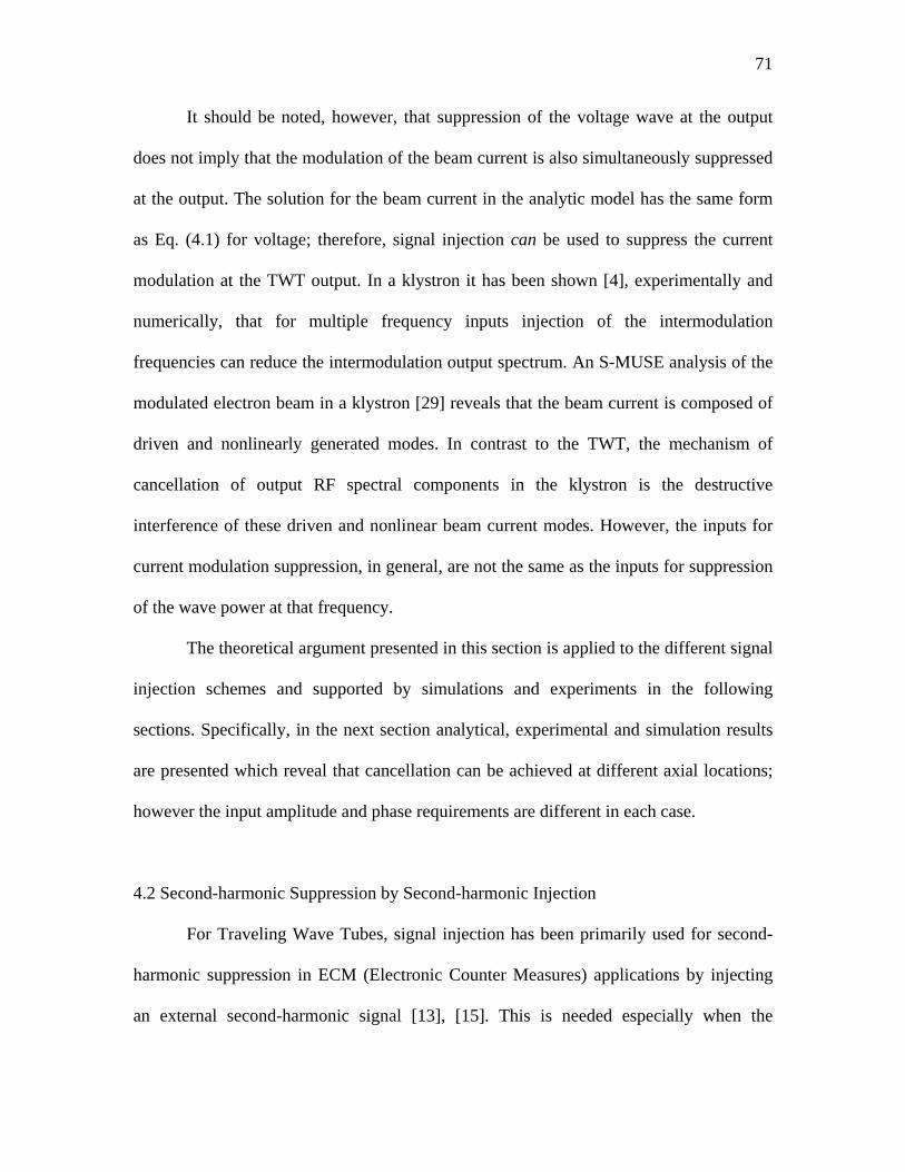
71
It should be noted, however, that suppression of the voltage wave at the output
does not imply that the modulation of the beam current is also simultaneously suppressed
at the output. The solution for the beam current in the analytic model has the same form
as Eq. (4.1) for voltage; therefore, signal injection can be used to suppress the current
modulation at the TWT output. In a klystron it has been shown [4], experimentally and
numerically, that for multiple frequency inputs injection of the intermodulation
frequencies can reduce the intermodulation output spectrum. An S-MUSE analysis of the
modulated electron beam in a klystron [29] reveals that the beam current is composed of
driven and nonlinearly generated modes. In contrast to the TWT, the mechanism of
cancellation of output RF spectral components in the klystron is the destructive
interference of these driven and nonlinear beam current modes. However, the inputs for
current modulation suppression, in general, are not the same as the inputs for suppression
of the wave power at that frequency.
The theoretical argument presented in this section is applied to the different signal
injection schemes and supported by simulations and experiments in the following
sections. Specifically, in the next section analytical, experimental and simulation results
are presented which reveal that cancellation can be achieved at different axial locations;
however the input amplitude and phase requirements are different in each case.
4.2 Second-harmonic Suppression by Second-harmonic Injection
For Traveling Wave Tubes, signal injection has been primarily used for second-
harmonic suppression in ECM (Electronic Counter Measures) applications by injecting
an external second-harmonic signal [13], [15]. This is needed especially when the
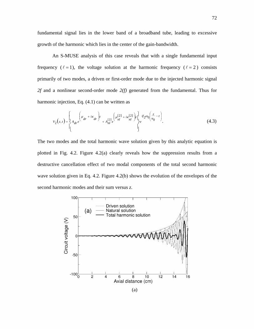
72
fundamental signal lies in the lower band of a broadband tube, leading to excessive
growth of the harmonic which lies in the center of the gain-bandwidth.
An S-MUSE analysis of this case reveals that with a single fundamental input
frequency ( 1= ), the voltage solution at the harmonic frequency ( 2= ) consists
primarily of two modes, a driven or first-order mode due to the injected harmonic signal
2f and a nonlinear second-order mode 2(f) generated from the fundamental. Thus for
harmonic injection, Eq. (4.1) can be written as
( )⎟⎟
⎠
⎞
⎜⎜
⎝
⎛−⎟⎟
⎠
⎞⎜⎜⎝
⎛+
+⎟⎟⎠
⎞⎜⎜⎝
⎛+
=
⎪⎭
⎪⎬
⎫
⎪⎩
⎪⎨
⎧ tuzif
ez
nli
nlenlA
zdr
idr
edrAtzV 002]2[]2[
,2]2[
ωκµκµ. (4.3)
The two modes and the total harmonic wave solution given by this analytic equation is
plotted in Fig. 4.2. Figure 4.2(a) clearly reveals how the suppression results from a
destructive cancellation effect of two modal components of the total second harmonic
wave solution given in Eq. 4.2. Figure 4.2(b) shows the evolution of the envelopes of the
second harmonic modes and their sum versus z.
(a)

73
(b)
FIG. 4.2 Illustration of second harmonic suppression by second harmonic injection in a TWT using the analytic solution given in Eq. (4.3). Destructive interference of the driven and nonlinear harmonic wave modes results in cancellation of the total solution at a single axial location. The two modes and their sum is shown in (a) on a linear scale while (b) shows component and sum envelope magnitudes on a log scale.
The nonlinear mode has a larger growth rate, approximately twice that of the
driven term [33]. Hence, it can be seen that the driven mode dominates the solution prior
to cancellation, while the nonlinearly generated (or natural) mode dominates after the
cancellation position. A plot of circuit voltage phase would show an abrupt change of
180° at the cancellation point [29]. Clearly, due to different growth rates and wavelengths
of the two modes, these terms are unable to sum to zero for all axial positions.
Experiments to validate this theory were conducted on the XWING tube. A single
fundamental frequency at 2 GHz with 15 dBm of input power was used to drive the tube.
The second harmonic for this frequency, 4 GHz, lies almost in the center of the gain-
bandwidth (Fig. 3.9) for the XWING TWT. With choice of this input frequency, the
output power (with no injection) was 36 dBm for 2 GHz and 24 dBm for 4 GHz. When
an external 4 GHz signal was injected and its amplitude and phase optimized for
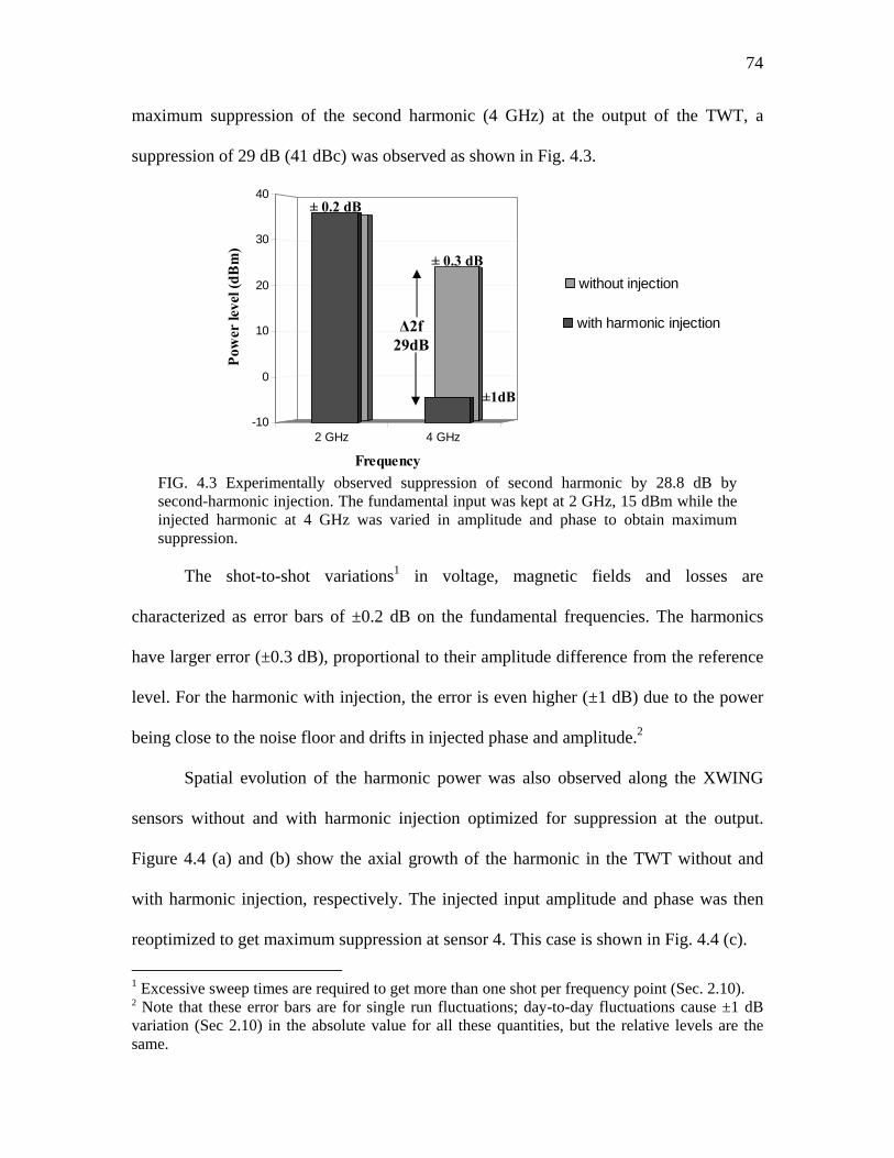
74
maximum suppression of the second harmonic (4 GHz) at the output of the TWT, a
suppression of 29 dB (41 dBc) was observed as shown in Fig. 4.3.
2 GHz 4 GHz
harm
onic
ectio
n
-10
0
10
20
30
40
Pow
er le
vel (
dBm
)
Frequency FIG. 4.3 Experimentally observed suppression of second harmonic by 28.8 dB by second-harmonic injection. The fundamental input was kept at 2 GHz, 15 dBm while the injected harmonic at 4 GHz was varied in amplitude and phase to obtain maximum suppression.
The shot-to-shot variations1 in voltage, magnetic fields and losses are
characterized as error bars of ±0.2 dB on the fundamental frequencies. The harmonics
have larger error (±0.3 dB), proportional to their amplitude difference from the reference
level. For the harmonic with injection, the error is even higher (±1 dB) due to the power
being close to the noise floor and drifts in injected phase and amplitude.2
Spatial evolution of the harmonic power was also observed along the XWING
sensors without and with harmonic injection optimized for suppression at the output.
Figure 4.4 (a) and (b) show the axial growth of the harmonic in the TWT without and
with harmonic injection, respectively. The injected input amplitude and phase was then
reoptimized to get maximum suppression at sensor 4. This case is shown in Fig. 4.4 (c).
1 Excessive sweep times are required to get more than one shot per frequency point (Sec. 2.10). 2 Note that these error bars are for single run fluctuations; day-to-day fluctuations cause ±1 dB variation (Sec 2.10) in the absolute value for all these quantities, but the relative levels are the same.
∆2f 29dB
± 0.2 dB
±1dB
± 0.3 dB
with harmonic injection
with
h inj
without injection

75
(a)
(b)
(c)
FIG. 4.4 Experimental and numerical evolution of second-harmonic (a) without injection, (b) with harmonic injection obtaining 29 dB suppression at output, and (c) with harmonic injection obtaining 31 dB suppression at sensor 4.
76
In Fig. 4.4, experimental data are also compared to predictions from the LATTE
“large signal code” [29, 32] which is based on the same starting equations as the
analytically solvable S-MUSE model. It is more appropriate to use LATTE rather than
the analytical solution to S-MUSE for this comparison; so that experimental details such
as an attenuating sever between two sections of the helix slow-wave circuit may be
accounted for.
Comparable suppressions were obtained at the output (29 dB) and at sensor 4 (31
dB). While measurements of injected phase could not be done easily for this pulsed high
frequency wave, the optimum injected amplitudes were recorded as 0.1 dBm and -2.4
dBm respectively. Therefore, ~2.5 dB higher power was required to suppress the
harmonic at the output than at sensor 4, which is in agreement with the gain between the
two taps (~3 dB) as seen in Fig. 4.4(a). The experimental results reveal that maximum
suppression is achieved at only a single axial location, and that the optimum injected
amplitude and phase requirements are different for suppression at the different axial
locations. Thus, the experiments confirm the theoretical principle of Eq. (4.3) that the
resultant harmonic wave consists of two modes with different growth rates and
wavelengths.
The amount of suppression achieved experimentally is limited by the resolution
bandwidths of the synthesizers and detectors, and the precision to which injected
amplitude and phase can be tuned to match the optimum values. A sensitivity analysis of
signal injection schemes is presented in Section 4.5. Theoretically and in simulations, a
much higher suppression can be obtained by fine-tuning the input parameters. Note
however that complete cancellation is still not possible since the complete solution [29]

77
also contains additional non-dominant (not exponentially growing) wave solution modes
at the harmonic frequency. In Fig. 4.4 simulations, precision of input amplitude and
phase was limited to match the amount of suppression observed experimentally.
The differences between the experimental measurements and the theoretical
curves produced by LATTE in Fig. 4.4 are readily accounted for by the fact that LATTE
is a 1-D code. The XWING TWT has a high space charge beam and several other
features that make it sensitive to three-dimensional effects. These effects can include
beam scalloping, radial expansion of bunches, and beam rotational velocity. Further,
repeated runs revealed that error allowances of approximately ±1 dB should be assumed
for the experimental data values, due to day-to-day variations in cathode conditioning. In
spite of these factors, the experiment and theory are in very good qualitative agreement.
4.3 Fundamental Enhancement by Second-Harmonic Injection
While optimized harmonic injection can suppress the second harmonic at the
output, earlier work [13], [15] and ECM applications focus on enhancing fundamental
power and efficiency with second-harmonic injection. This is also expected from the S-
MUSE model since the fundamental frequency also has a solution similar to Eq. (4.3) for
second-harmonic that can be written as
( )⎟⎟
⎠
⎞
⎜⎜
⎝
⎛−⎟⎟
⎠
⎞⎜⎜⎝
⎛+
+⎟⎟⎠
⎞⎜⎜⎝
⎛+
=
⎪⎭
⎪⎬
⎫
⎪⎩
⎪⎨
⎧ tuzif
ez
nli
nlenlA
zdr
idr
edrAtzV 001]2[]2[
,1]2[
ωκµκµ (4.4)
The fundamental solution essentially consists of the driven mode (f) and a second-order
nonlinear mode formed by beating of the injected harmonic with the driven fundamental
(2f) – (f). Thus, the amplitude and phase of the injected harmonic can be adjusted to
78
obtain constructive interference of the two modes and increase the power at the
fundamental.
Experimental investigations were done by varying the harmonic phase and
observing the fundamental and second-harmonic output levels. The input fundamental
was again set at 2 GHz, 15 dBm and the second harmonic at 4 GHz. Figure 4.5 shows
this relation on a log and linear scale.
-10.0
-5.0
0.0
5.0
10.0
15.0
20.0
25.0
30.0
35.0
40.0
0 60 120 180 240 300 360Relative Injected Harmonic phase (deg)
Out
put p
ower
(dB
m)
2 GHz with injection4 GHz with injection2 GHz w/o injection4 GHz w/o injection
(a)
0.0
0.5
1.0
1.5
2.0
2.5
3.0
3.5
0 60 120 180 240 300 360Relative Injected Harmonic phase (deg)
Out
put p
ower
(W)
2 GHz with injection4 GHz with injection2 GHz w/o injection4 GHz w/o injection
(b)
FIG. 4.5 Variation of output fundamental and harmonic power with second-harmonic injection depicted on (a) log scale and (b) linear scale showing that second-harmonic injection provides not only suppression of the second-harmonic but also improves the fundamental output.
79
Clearly, the fundamental power also varies with injected second harmonic phase.
Thus, harmonic injection not only suppresses the second harmonic at the output, but also
boosts the fundamental efficiency. The fundamental power was boosted by ~8% in the
experiment. Thus, second-harmonic injection is capable of enhancing fundamental power
and efficiency. Optimization of both injected amplitude and phase may lead to further
efficiency improvement.
It should also be noted that since in this experiment the injected harmonic
amplitude is fixed at the optimum suppression value, its value should be approximately
the same as the nonlinearly generated harmonic. This also implies that the maximum
increase in the harmonic power level with phase should be ~6dB (twice the voltage and
four times the power without harmonic injection). This is found to be the case as
observed in Fig. 4.5(a).
The experimental results also reveal that the fundamental power is maximized for
approximately the same injected harmonic phase that causes maximum suppression in the
output second harmonic. Though this would be a desired feature and may seem
intuitively correct, the S-MUSE model for the two cases predicts that in general, the input
phase requirement for maximum suppression of the second-harmonic may not necessarily
correspond to the phase required for maximum increase in fundamental. This is because
simultaneous minimization of (4.3) and maximization of (4.4) with one amplitude and
phase may not be possible as the terms involved have different growth rates and phase
velocities.
To verify that the experimental observation is not unique to the choice of our
frequencies, the same experiment was repeated for a 1.5 GHz, 15 dBm fundamental input

80
with 3.0 GHz second-harmonic injection. With -10.1 dBm of injected harmonic power,
maximum harmonic suppression of 31dB was obtained at the output. However, output
power vs. injected phase results shown in Fig. 4.6 still show discrepancy between the
experimental observations and theory since maximum harmonic suppression and
fundamental enhancement are obtained for same value of injected phase.
-20
-15
-10
-5
0
5
10
15
20
25
30
0 60 120 180 240 300 360
Relative Injected Harmonic phase (degs)
Out
put p
ower
(dB
m)
1.5 GHz with injection3.0 GHz with injection1.5 GHz w/o injection3.0 GHz w/o injection
(a)
0
0.1
0.2
0.3
0.4
0.5
0 60 120 180 240 300 360
Relative Injected Harmonic phase (degs)
Out
put p
ower
(W)
1.5 GHz with injection3.0 GHz with injection1.5 GHz w/o injection3.0 GHz w/o injection
(b)
FIG. 4.6 Harmonic suppression and fundamental enhancement at XWING output for 1.5 GHz, 15 dBm drive on (a) log scale and (b) linear scale.
81
A similar measurement was then taken to suppress the second-harmonic at sensor
1 with 2 GHz, 15 dBm input. Since the harmonic power level at sensor 1 is pretty low,
limitations imposed by the resolution and noise floor of the spectrum analyzer allowed a
maximum harmonic suppression of 21dB at this location. Phase sensitivity measurements
shown in Fig. 4.7 reveal that the conditions for suppressing second-harmonic and
enhancing the fundamental are indeed different for this axial location.
20
21
22
23
24
25
26
27
28
0 60 120 180 240 300 360Relative Injected Harmonic phase (degs)
Out
put p
ower
f (d
Bm
)
-20
-15
-10
-5
0
5
10
15
20
Output pow
er 2f (dBm
)2 GHz with injection2 GHz w/o injection4 GHz with injection4 GHz w/o injection
(a)
0
0.1
0.2
0.3
0.4
0.5
0.6
0 60 120 180 240 300 360
Relative Injected Harmonic phase (degs)
Out
put p
ower
f (W
)
0.0
0.5
1.0
1.5
2.0
2.5
3.0
3.5
4.0
4.5
Output pow
er 2f (mW
)2 GHz with injection2 GHz w/o injection4 GHz with injection4 GHz w/o injection
(b)
FIG. 4.7 Harmonic suppression and fundamental enhancement at sensor 1 of XWING for 2.0 GHz, 15 dBm drive on (a) log scale and (b) linear scale. (Note: The axes for fundamental and harmonic power levels are separate due to smaller levels of harmonic at sensor 1).

82
Thus, in general, the injected harmonic amplitude and phase required for
suppressing harmonic and for boosting the fundamental are different. Depending on the
application, one or other can be achieved or an optimum set of parameters can be chosen
to satisfy both to some extent. In the XWING somehow the parameters match up to yield
same amplitude and phase requirement for suppression of harmonic and fundamental
enhancement at the output. However, it is sensitive to the axial location.
While the principle has been addressed here, the simulations using LATTE were
not found to agree in phase with the experimental data. Many issues need to be addressed
here including 3D or other effects missing in the LATTE model, uniformity of phase shift
introduced by the phase shifter, actual phase shift seen by the beam due to any unforeseen
capacitive coupling etc.
4.4 3IM Suppression by Second-harmonic Injection
Apart from suppressing harmonics, intermodulation suppression is important
primarily for multi-carrier communication applications. The intermodulation products
lead to spectral regrowth around the fundamentals thus causing in-band distortion and
cross-talk between adjacent channels. Linearization of the amplifier primarily aims to
suppress the third-order products or 3IMs since these lie closest to the fundamentals and
are also the strongest.
Second-harmonic injection can also be used to suppress the 3IMs. For a two-tone
case, injection of harmonics of the two fundamentals leads to generation of additional
modes at the 3IM frequencies (2fa-fb, 2fb-fa) due to nonlinear beating of the injected
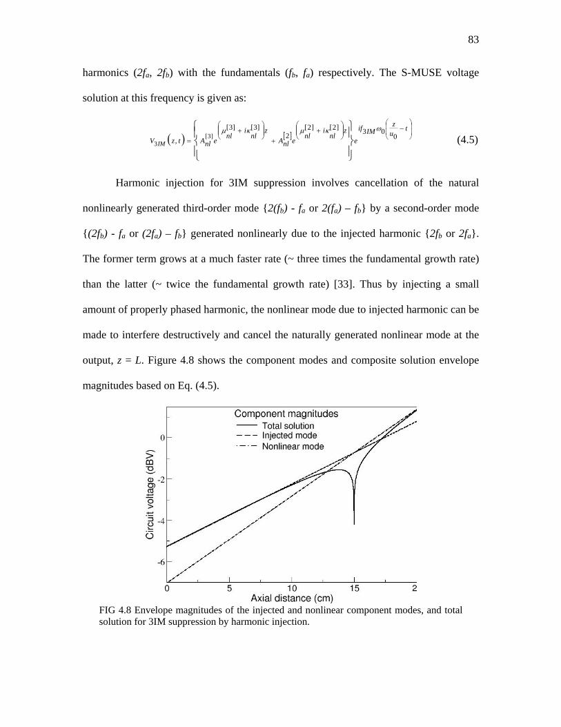
83
harmonics (2fa, 2fb) with the fundamentals (fb, fa) respectively. The S-MUSE voltage
solution at this frequency is given as:
( ) [ ] ⎟⎟
⎠
⎞
⎜⎜
⎝
⎛−⎟⎟
⎠
⎞⎜⎜⎝
⎛+
+⎟⎟⎠
⎞⎜⎜⎝
⎛+
=
⎪⎭
⎪⎬⎫
⎪⎩
⎪⎨⎧ t
uz
IMif
ez
nli
nlenlA
znl
inl
enlAtzV IM0
03]2[]2[2
]3[]3[
,]3[
3
ωκµκµ (4.5)
Harmonic injection for 3IM suppression involves cancellation of the natural
nonlinearly generated third-order mode 2(fb) - fa or 2(fa) – fb by a second-order mode
(2fb) - fa or (2fa) – fb generated nonlinearly due to the injected harmonic 2fb or 2fa.
The former term grows at a much faster rate (~ three times the fundamental growth rate)
than the latter (~ twice the fundamental growth rate) [33]. Thus by injecting a small
amount of properly phased harmonic, the nonlinear mode due to injected harmonic can be
made to interfere destructively and cancel the naturally generated nonlinear mode at the
output, z = L. Figure 4.8 shows the component modes and composite solution envelope
magnitudes based on Eq. (4.5).
FIG 4.8 Envelope magnitudes of the injected and nonlinear component modes, and total solution for 3IM suppression by harmonic injection.
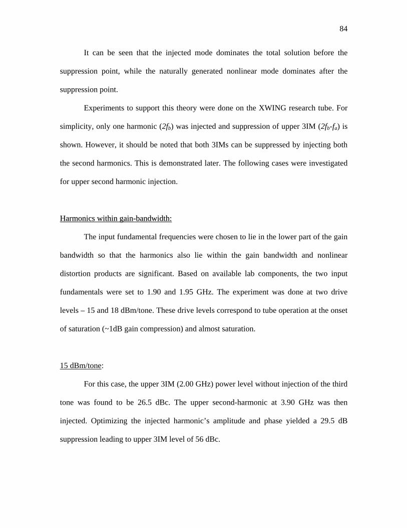
84
It can be seen that the injected mode dominates the total solution before the
suppression point, while the naturally generated nonlinear mode dominates after the
suppression point.
Experiments to support this theory were done on the XWING research tube. For
simplicity, only one harmonic (2fb) was injected and suppression of upper 3IM (2fb-fa) is
shown. However, it should be noted that both 3IMs can be suppressed by injecting both
the second harmonics. This is demonstrated later. The following cases were investigated
for upper second harmonic injection.
HHaarrmmoonniiccss wwiitthhiinn ggaaiinn--bbaannddwwiiddtthh::
The input fundamental frequencies were chosen to lie in the lower part of the gain
bandwidth so that the harmonics also lie within the gain bandwidth and nonlinear
distortion products are significant. Based on available lab components, the two input
fundamentals were set to 1.90 and 1.95 GHz. The experiment was done at two drive
levels – 15 and 18 dBm/tone. These drive levels correspond to tube operation at the onset
of saturation (~1dB gain compression) and almost saturation.
15 dBm/tone:
For this case, the upper 3IM (2.00 GHz) power level without injection of the third
tone was found to be 26.5 dBc. The upper second-harmonic at 3.90 GHz was then
injected. Optimizing the injected harmonic’s amplitude and phase yielded a 29.5 dB
suppression leading to upper 3IM level of 56 dBc.
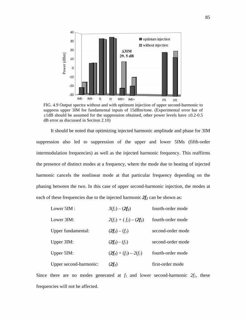
85
IM5- IM3- f1 f2 IM3+ IM5+ 2f1 2f2
-30
-20
-10
0
10
20
30
40
Pow
er (d
Bm
)
optimum injectionwithout injection
FIG. 4.9 Output spectra without and with optimum injection of upper second-harmonic to suppress upper 3IM for fundamental inputs of 15dBm/tone. (Experimental error bar of ±1dB should be assumed for the suppression obtained, other power levels have ±0.2-0.5 dB error as discussed in Seciton 2.10)
It should be noted that optimizing injected harmonic amplitude and phase for 3IM
suppression also led to suppression of the upper and lower 5IMs (fifth-order
intermodulation frequencies) as well as the injected harmonic frequency. This reaffirms
the presence of distinct modes at a frequency, where the mode due to beating of injected
harmonic cancels the nonlinear mode at that particular frequency depending on the
phasing between the two. In this case of upper second-harmonic injection, the modes at
each of these frequencies due to the injected harmonic 2f2 can be shown as:
Lower 5IM : 3(f1) – (2f2) fourth-order mode
Lower 3IM: 2(f1) + ( f2) – (2f2) fourth-order mode
Upper fundamental: (2f2) – (f2) second-order mode
Upper 3IM: (2f2) – (f1) second-order mode
Upper 5IM: (2f2) + (f2) – 2(f1) fourth-order mode
Upper second-harmonic: (2f2) first-order mode
Since there are no modes generated at f1 and lower second-harmonic 2f1, these
frequencies will not be affected.
∆3IM 29. 5 dB
86
Thus, the injected amplitude and phase can be optimized to either achieve
maximum suppression at a particular frequency or to obtain some desired suppression at
multiple frequencies.
18 dBm/tone:
With 18 dBm/tone, the upper 3IM level was 23dBc without injection. Injection of
the upper second-harmonic in this case reduced the 3IM power at the output by 32.4 dB.
IM5- IM3- f1 f2 IM3+ IM5+ 2f1 2f2
-30
-20
-10
0
10
20
30
40
Pow
er (d
Bm
)
optimum injectionwithout injection
FIG. 4.10 Output spectra without and with optimum injection of upper second-harmonic to suppress upper 3IM for fundamental inputs of 18dBm/tone. (Experimental error bar of ±1dB should be assumed for the suppression obtained, other power levels have ±0.2-0.5 dB error as discussed in Section 2.10)
The suppression obtained is higher in this case since the initial level without injection
was higher with higher drive, while the minimum obtainable power is still limited by the
resolution of the synthesizer and spectrum analyzer, and the initial 3IM level at TWT
input from preamplifiers. Again, some suppression of both 5IMs as well as the upper
harmonic is obtained.
Spatial evolution of the all the relevant spectral frequencies without injection and
with optimum injection was measured along the axial sensors in the XWING TWT for
the 15 dBm/tone case.
∆3IM 32. 4 dB
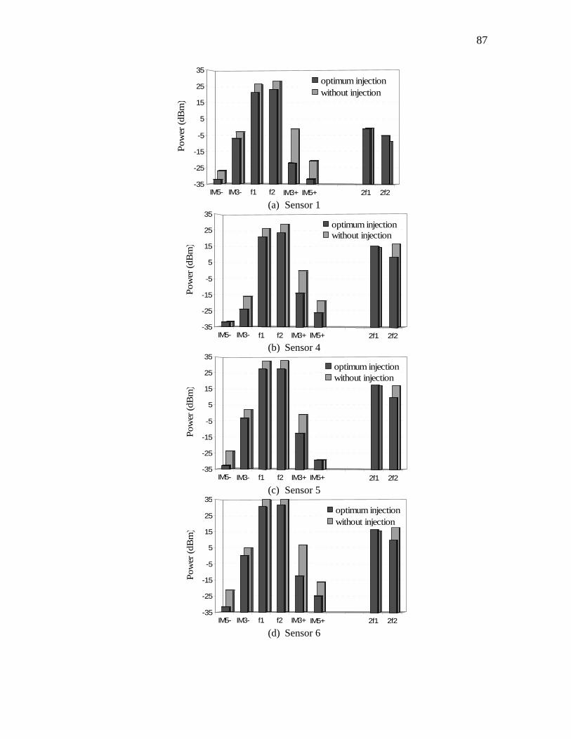
87
IM5- IM3- f1 f2 IM3+ IM5+ 2f1 2f2-35
-25
-15
-5
5
15
25
35
Pow
er (d
Bm
)
optimum injectionwithout injection
(a) Sensor 1
IM5- IM3- f1 f2 IM3+ IM5+ 2f1 2f2-35
-25
-15
-5
5
15
25
35
Pow
er (d
Bm
)
optimum injectionwithout injection
(b) Sensor 4
IM5- IM3- f1 f2 IM3+ IM5+ 2f1 2f2-35
-25
-15
-5
5
15
25
35
Pow
er (d
Bm
)
optimum injectionwithout injection
(c) Sensor 5
IM5- IM3- f1 f2 IM3+ IM5+ 2f1 2f2-35
-25
-15
-5
5
15
25
35
Pow
er (d
Bm
)
optimum injectionwithout injection
(d) Sensor 6
88
IM5- IM3- f1 f2 IM3+ IM5+ 2f1 2f2-35
-25
-15
-5
5
15
25
35
Pow
er (d
Bm
)
optimum injectionwithout injection
(e) Output
FIG. 4.11 Spatial evolution of the relevant spectral frequencies at (a) sensor 1, (b) sensor 4, (c) sensor 5, (d) sensor 6 and (e) output for harmonic injection to suppress upper 3IM.
The spatial evolution shows both constructive and destructive effects of the
nonlinear modes at the various frequencies due to injected signal beating with the
naturally generated nonlinear and driven modes.
While only the upper 3IM was examined in the previous experiments, it is
possible to suppress both upper and lower 3IMs by simultaneous injection of upper and
lower second-harmonic. Experimental measurements were taken for input frequencies of
1.90 and 1.95 GHz at 15 dBm/tone. Optimized injection of harmonics at 3.80 and 3.90
GHz resulted in 28.4 dB and 31.4 dB of suppression respectively for the lower and upper
3IMs at the output. The spectra measured at each sensor are shown in Fig. 4.12.
IM5- IM3- f1 f2 IM3+ IM5+ 2f1 2f2-30
-20
-10
0
10
20
30
40
Pow
er (d
Bm
)
optimum injectionwithout injection
(a) Input
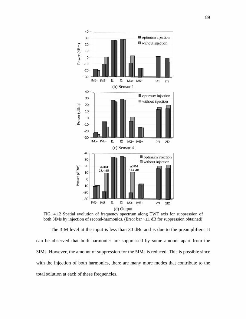
89
IM5- IM3- f1 f2 IM3+ IM5+ 2f1 2f2-30
-20
-10
0
10
20
30
40
Pow
er (d
Bm
)
optimum injectionwithout injection
(b) Sensor 1
IM5- IM3- f1 f2 IM3+ IM5+ 2f1 2f2-30
-20
-10
0
10
20
30
40
Pow
er (d
Bm
)
optimum injectionwithout injection
(c) Sensor 4
IM5- IM3- f1 f2 IM3+ IM5+ 2f1 2f2-30
-20
-10
0
10
20
30
40
Pow
er (d
Bm
)
optimum injectionwithout injection
(d) Output
FIG. 4.12 Spatial evolution of frequency spectrum along TWT axis for suppression of both 3IMs by injection of second-harmonics. (Error bar ~±1 dB for suppression obtained)
The 3IM level at the input is less than 30 dBc and is due to the preamplifiers. It
can be observed that both harmonics are suppressed by some amount apart from the
3IMs. However, the amount of suppression for the 5IMs is reduced. This is possible since
with the injection of both harmonics, there are many more modes that contribute to the
total solution at each of these frequencies.
∆3IM 31.4 dB
∆3IM 28.4 dB

90
Thus, it has been established that both the 3IMs can be suppressed by injecting
the corresponding harmonics. However for simplicity of set-up and equipment
limitations, the rest of the techniques investigated experimentally focus on suppression of
the upper 3IM only.
4.5 3IM Suppression by 3IM Injection
Injection of a second-harmonic signal to suppress the 3IM frequency suggests the
more obvious scheme of injecting the 3IM frequency itself. In fact, the conventional
predistortion linearizer works on this principle and can be thought of as a generator of
IMD (Inter-Modulation Distortion) products whose amplitudes and phases are adjusted
according to an inverse transfer characteristic to cancel the nonlinearly generated IMDs
[17]. Thus, it is insightful to investigate this scheme and compare with second-harmonic
injection for 3IM suppression.
For a two-tone input at fa, fb with injection of one or both 3IMs at 2fb-fa and/or 2fa-
fb, the S-MUSE solution at the 3IM frequencies is given as:
( ) [ ] ⎟⎟
⎠
⎞
⎜⎜
⎝
⎛−⎟⎟
⎠
⎞⎜⎜⎝
⎛+
+⎟⎟⎠
⎞⎜⎜⎝
⎛+
=
⎪⎭
⎪⎬
⎫
⎪⎩
⎪⎨
⎧ tuz
IMif
ez
nli
nlenlA
zdr
idr
edrAtzV IM0
03]3[]3[3
,3
ωκµκµ (4.6)
3IM injection for 3IM suppression involves cancellation of the natural nonlinearly
generated third-order mode 2(fb) - fa or 2(fa) – fb by a first-order injected mode 2fb - fa
or 2fa – fb due to injected signal at the 3IM frequency. Again, the growth rate of the
third-order natural mode (approximately three times the fundamental) is greater than the
first-order driven mode (~ same as the fundamental). Figure 4.13 shows the magnitudes
of the component modes and total solution of the circuit voltage envelope.
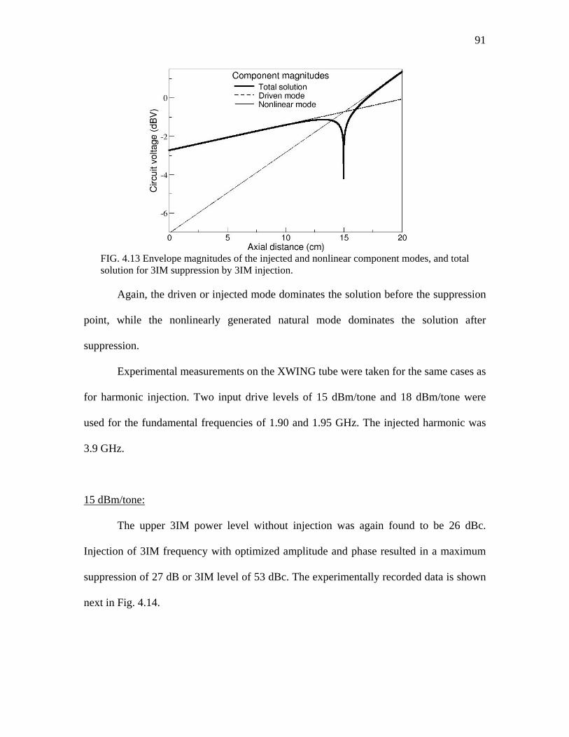
91
FIG. 4.13 Envelope magnitudes of the injected and nonlinear component modes, and total solution for 3IM suppression by 3IM injection.
Again, the driven or injected mode dominates the solution before the suppression
point, while the nonlinearly generated natural mode dominates the solution after
suppression.
Experimental measurements on the XWING tube were taken for the same cases as
for harmonic injection. Two input drive levels of 15 dBm/tone and 18 dBm/tone were
used for the fundamental frequencies of 1.90 and 1.95 GHz. The injected harmonic was
3.9 GHz.
15 dBm/tone:
The upper 3IM power level without injection was again found to be 26 dBc.
Injection of 3IM frequency with optimized amplitude and phase resulted in a maximum
suppression of 27 dB or 3IM level of 53 dBc. The experimentally recorded data is shown
next in Fig. 4.14.

92
IM5- IM3- f1 f2 IM3+ IM5+ 2f1 2f2-30
-20
-10
0
10
20
30
40
Pow
er (d
Bm
)
optimum injectionwithout injection
FIG. 4.14 Output spectra without and with optimum injection of upper 3IM frequency to suppress upper 3IM for fundamental inputs of 15 dBm/tone. (Experimental error bar of ±1dB should be assumed for the suppression obtained, other power levels have ±0.2-0.5 dB error as discussed in Seciton 2.10)
In this case in addition to the suppression of the upper 3IM, the upper 5IM is also
suppressed. However, none of the harmonic is suppressed and the lower 5IM in fact
comes up. This destructive and constructive cancellation at the various frequencies is
explainable since there is a mode at each of these frequencies formed by beating of the
injected 3IM signal as shown below:
Lower 5IM: 2(f1) – (2f2 – f1) third-order mode
Upper 3IM: (2f2 – f1) first-order mode
Upper 5IM: (2f2 – f1) + (f2) – (f1) third-order mode
The phasing relationship between the modes due to the injected signal and the naturally
generated modes determines the nature of the effect – destructive or constructive. In
general, it has been found [17] that the predistortion equalizers, which work by injecting
3IMs, usually cause the higher-order intermods to increase. This is observed
experimentally for atleast one of the 5IMs for the 15 dBm/tone case, while the upper
second-harmonic is found to come up for 18 dBm/tone as shown next.
∆3IM 27 dB
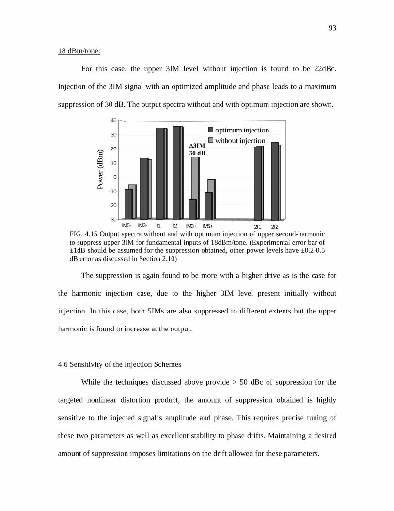
93
18 dBm/tone:
For this case, the upper 3IM level without injection is found to be 22dBc.
Injection of the 3IM signal with an optimized amplitude and phase leads to a maximum
suppression of 30 dB. The output spectra without and with optimum injection are shown.
IM5- IM3- f1 f2 IM3+ IM5+ 2f1 2f2-30
-20
-10
0
10
20
30
40
Pow
er (d
Bm
)
optimum injectionwithout injection
FIG. 4.15 Output spectra without and with optimum injection of upper second-harmonic to suppress upper 3IM for fundamental inputs of 18dBm/tone. (Experimental error bar of ±1dB should be assumed for the suppression obtained, other power levels have ±0.2-0.5 dB error as discussed in Section 2.10)
The suppression is again found to be more with a higher drive as is the case for
the harmonic injection case, due to the higher 3IM level present initially without
injection. In this case, both 5IMs are also suppressed to different extents but the upper
harmonic is found to increase at the output.
4.6 Sensitivity of the Injection Schemes
While the techniques discussed above provide > 50 dBc of suppression for the
targeted nonlinear distortion product, the amount of suppression obtained is highly
sensitive to the injected signal’s amplitude and phase. This requires precise tuning of
these two parameters as well as excellent stability to phase drifts. Maintaining a desired
amount of suppression imposes limitations on the drift allowed for these parameters.
∆3IM 30 dB

94
Experimental measurements were taken to study the sensitivity of the suppression
to injected amplitude and phase. This was done for second-harmonic injection with
fundamental frequencies of 1.90 and 1.95 GHz at 18 dBm/.tone. Since changing injected
amplitude by adjusting attenuator causes the phase to also change, a phase sweep was
done at each injected amplitude level.
FIG. 4.16 Sensitivity of suppression of signal injection to injected amplitude and phase. The case shown here is for second-harmonic injection for fundamentals 1.90 and 1.95 GHz at 18 dBm/tone.
As can be seen, the amount of suppression obtained is very sensitive to the
precision of injected amplitude and phase. While a suppression of ~ 20 dB is guaranteed
for variations < +/-1dB in amplitude and up to 5° in phase, further suppression depends
on fine tuning of these parameters. Sensitivity measurements with other signal injection
schemes also exhibit similar behavior.
Relative Injected Harmonic Phase (degrees)
Relative Injected Harmonic Amplitude (dBm)
IM3 Power w/o inj 13.5 dBm

95
One experimental difficulty here is that changing the input amplitude by varying
the attenuator also changes the phase of the injected signal. Thus, phase has to be
reoptimized every time amplitude is changed. With the given equipment, this presents a
challenge to the fine tuning of these parameters and thus the amount of suppression
achieved.
4.7 3IM Suppression by Two-frequency (3IM + Second-Harmonic) Injection
The previous section describes the sensitivity of suppression to injected signal’s
amplitude and phase. While some desired suppression can be obtained by limiting the
drifts in amplitude and phase to a small range of values, obtaining and maintaining a high
level of suppression requires precise control and stability of the two parameters. In
practice high phase precision may be difficult to achieve, particularly at GHz frequencies.
To avoid the need of precise phase control, a scheme based on simultaneous injection of
second-harmonic and 3IM is presented. This scheme allows the phase of the two injected
tones to be arbitrary fixed value (within a certain wide range), while their amplitudes are
adjusted to obtain suppression.
For this two-frequency injection scheme with injection of second-harmonic 2fb
(and/or 2fa) and 3IM 2fb – fa (and/or 2fa – fb), the S-MUSE solution at the 3IM frequency
2fb – fa (and/or 2fa – fb) is given as
( ) [ ] [ ] ⎟⎟
⎠
⎞
⎜⎜
⎝
⎛−⎟⎟
⎠
⎞⎜⎜⎝
⎛+
+⎟⎟⎠
⎞⎜⎜⎝
⎛+
+⎟⎟⎠
⎞⎜⎜⎝
⎛+
=
⎪⎭
⎪⎬
⎫
⎪⎩
⎪⎨
⎧ tuz
IMif
ez
nli
nlenlA
znl
inl
enlAz
dri
dredrAtzV IM
003]3[]3[
3]2[]2[
2,3
ωκµκµκµ (4.7)
Thus, two-frequency injection involves cancellation of the third-order naturally
generated nonlinear mode 2(fb) – fa or 2(fa) – fb with a combination of a second-order

96
nonlinear mode due to injected second-harmonic (2fb) – fa or (2fa) – fb and a first-order
or driven mode due to injected 3IM 2fb – fa or 2fa – fb.
To understand the concept better, these three modes are plotted in a phasor
diagram at the output of the TWT.
FIG. 4.17 Phasor diagram at TWT output for the different modes in a two-frequency (3IM + second-harmonic) injection scheme. The resultant of the two modes due to injected harmonic and 3IM can cancel the naturally produced 3IM by adjusting the length or amplitude of the phasors as long as the phase of the two injected modes lie above the dashed line.
As can be seen from Fig. 4.17, cancellation of the naturally produced 3IM with the
resultant 3IM requires them to be equal in amplitude and opposite in phase. The resultant
3IM can be adjusted in both magnitude and phase by adjusting only the amplitudes of the
two component modes due to injected harmonic and injected 3IM. This is possible as
long as the phases of the two injected modes are fixed and lie above the dashed line in
Fig. 4.17 i.e within 90° of the desired resultant direction. A better range would be ~60°
since larger angles imply more injected power. This range is also suggested in [12].
Notice that suppression can still be obtained if one injected mode lies above and the other
below the dashed line in the opposite quadrant and within 180°, but would again require
high injected powers.
IInnjjeecctteedd 33IIMM
RReessuullttaanntt 33IIMM
33IIMM dduuee ttoo iinnjjeecctteedd hhaarrmmoonniicc
NNaattuurraallllyy pprroodduucceedd 33IIMM
IImm
RRee
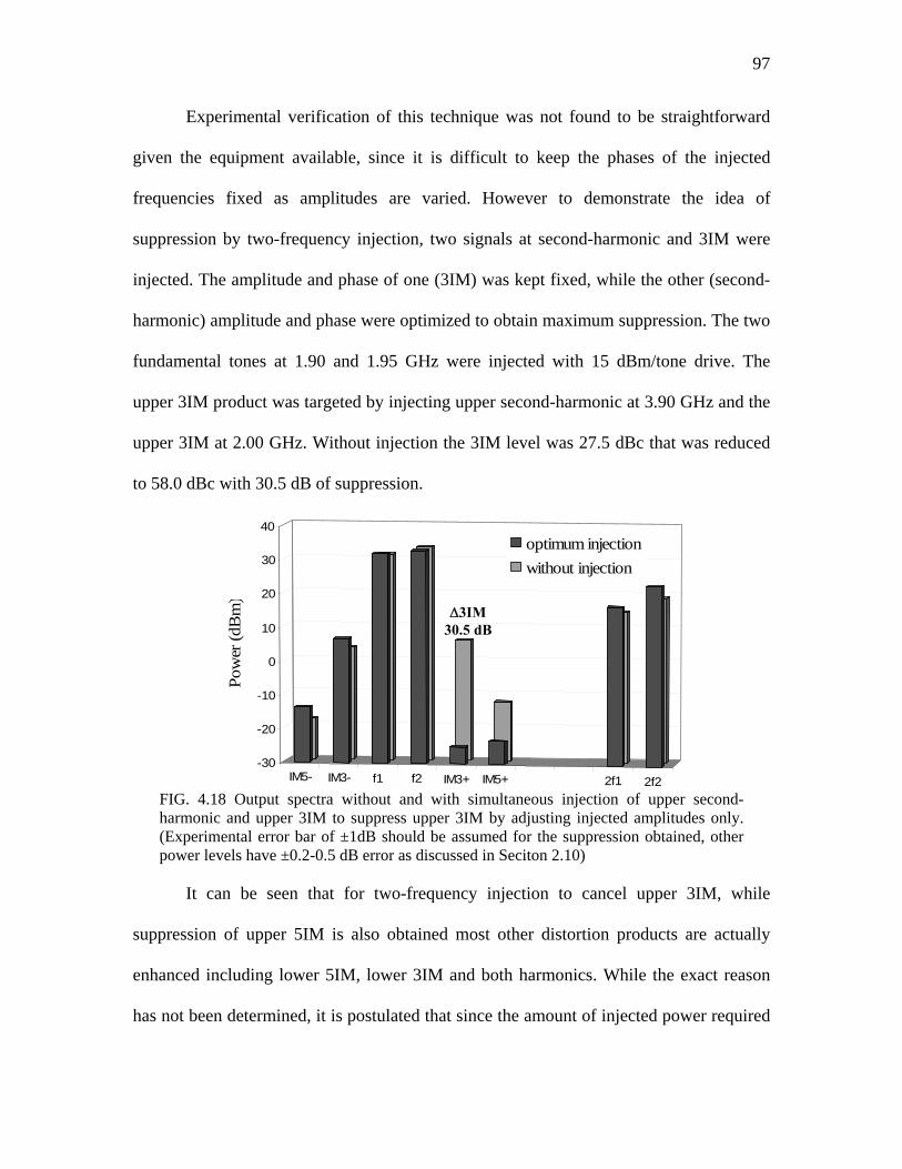
97
Experimental verification of this technique was not found to be straightforward
given the equipment available, since it is difficult to keep the phases of the injected
frequencies fixed as amplitudes are varied. However to demonstrate the idea of
suppression by two-frequency injection, two signals at second-harmonic and 3IM were
injected. The amplitude and phase of one (3IM) was kept fixed, while the other (second-
harmonic) amplitude and phase were optimized to obtain maximum suppression. The two
fundamental tones at 1.90 and 1.95 GHz were injected with 15 dBm/tone drive. The
upper 3IM product was targeted by injecting upper second-harmonic at 3.90 GHz and the
upper 3IM at 2.00 GHz. Without injection the 3IM level was 27.5 dBc that was reduced
to 58.0 dBc with 30.5 dB of suppression.
IM5- IM3- f1 f2 IM3+ IM5+ 2f1 2f2-30
-20
-10
0
10
20
30
40
Pow
er (d
Bm
)
optimum injectionwithout injection
FIG. 4.18 Output spectra without and with simultaneous injection of upper second-harmonic and upper 3IM to suppress upper 3IM by adjusting injected amplitudes only. (Experimental error bar of ±1dB should be assumed for the suppression obtained, other power levels have ±0.2-0.5 dB error as discussed in Seciton 2.10)
It can be seen that for two-frequency injection to cancel upper 3IM, while
suppression of upper 5IM is also obtained most other distortion products are actually
enhanced including lower 5IM, lower 3IM and both harmonics. While the exact reason
has not been determined, it is postulated that since the amount of injected power required
∆3IM 30.5 dB
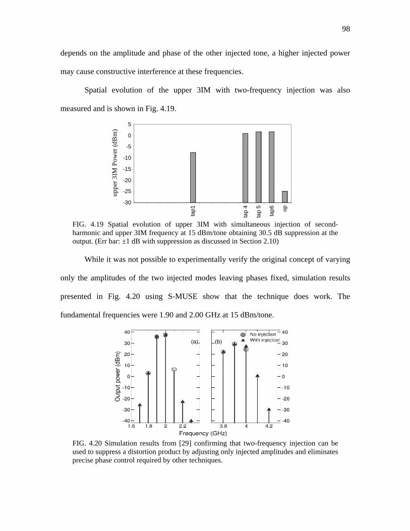
98
depends on the amplitude and phase of the other injected tone, a higher injected power
may cause constructive interference at these frequencies.
Spatial evolution of the upper 3IM with two-frequency injection was also
measured and is shown in Fig. 4.19.
tap1
tap
4
tap
5
tap6 op
-30
-25
-20
-15
-10
-5
0
5
uppe
r 3IM
Pow
er (d
Bm
)
FIG. 4.19 Spatial evolution of upper 3IM with simultaneous injection of second-harmonic and upper 3IM frequency at 15 dBm/tone obtaining 30.5 dB suppression at the output. (Err bar: ±1 dB with suppression as discussed in Section 2.10)
While it was not possible to experimentally verify the original concept of varying
only the amplitudes of the two injected modes leaving phases fixed, simulation results
presented in Fig. 4.20 using S-MUSE show that the technique does work. The
fundamental frequencies were 1.90 and 2.00 GHz at 15 dBm/tone.
FIG. 4.20 Simulation results from [29] confirming that two-frequency injection can be used to suppress a distortion product by adjusting only injected amplitudes and eliminates precise phase control required by other techniques.

99
4.8 Bandwidth of Suppression
It is instructive to determine the bandwidth over which suppression is effective. A
higher bandwidth is desired since it implies that suppression is not too influenced by
frequency drifts or small changes in carrier frequency.
Experimental measurement of frequency sensitivity of suppression was done for
the second harmonic injection scheme by varying the frequency fa and keeping fb fixed,
and injecting 2fb to suppress upper 3IM 2fb - fa. Injection was optimized for the
fundamental frequencies of 1.90 and 1.95 GHz with injection of a 3.90 GHz harmonic.
The fundamental at 1.90 GHz was then varied over a wide range and the suppression
observed. Experimental data for two trials is shown in Fig. 4.21.
-35
-30
-25
-20
-15
-10
-5
0
1.00 1.15 1.30 1.45 1.60 1.75 1.90 2.05 2.20 2.35 2.50
fa frequency (GHz)
uppe
r 3IM
Sup
pres
sion
n (d
B)
Trial 1Trial 2
FIG. 4.21 Sensitivity of upper 3IM suppression to lower fundamental frequency variation for second-harmonic injection scheme. Injection was optimized for fa = 1.90 GHz. (Experimental error bars are estimated to be ±1 dB with suppression (Section 2.10))
It can be seen that though maximum suppression is obtained at the optimization
frequency, the overall bandwidth of effective suppression is pretty high. A suppression of
> 20 dB is possible over almost a GHz change in the lower fundamental frequency. While
a theoretical investigation and reasoning is necessary to draw any final conclusions, this
fb (1.95 GHz) fa (1.90 GHz)
100
observation suggests that the second-harmonic is mainly responsible for generating
distortion products. While the suppression is quite sensitive to injected harmonic
amplitude and phase (section 4.6), as long as the second-harmonic remains fixed, the
suppression is relatively insensitive to drifts in the fundamental frequency it beats with to
form intermodulation distortion products.
4.9 Comparison of the Schemes
The experimental results indicate that comparable suppression of up to ~30 dB is
possible at a single frequency using any of the signal injection schemes discussed in this
chapter. The choice of the injection scheme depends on various factors including the
effect on higher-order intermods, power requirements, simplicity and ease of
implementation. The experimental measurements provide some guidelines in this respect.
While more detailed investigations are needed to draw general conclusions, some
hypothesis based on observations from experimental data and theoretical arguments is
presented here.
It was observed that for 3IM injection scheme, some higher order intemods and
harmonics are adversely affected while trying to suppress third-order intermods (Figs.
4.14 and 4.15). This is also a general observation for predistortion equalizers that work
on the principle of 3IM injection [17]. On the other hand, harmonic injection results in
some suppression of higher-order intermods as well as the harmonics (Figs. 4.9 and
4.10). This is desired for communication applications since, although we want to target
the third-order intermods that are strongest amongst all intermods and closest to the
fundamentals, the overall spurious frequency content also needs to be low. The two-
frequency injection scheme involving simultaneous injection of second-harmonic and
101
3IM proved to be the worst in effecting other frequencies adversely, however a judicious
choice of the fixed injected phases might improve this behavior by reducing the amount
of injected amplitude required. While the amount of suppression achieved for higher-
order intermods and harmonics will depend on the phasing between the different
frequencies and modes, the fact that similar observations are reported for equalizers [17]
suggests that it may be a general phenomenon and is not unique to the XWING tube.
Another supporting notion for the second-harmonic injection not affecting the higher-
order intermods as much as 3IM injection, is that the order of the injected mode at a
higher-order intermod frequency is lower for 3IM injection than for second-harmonic
injection. For example, the injected modes at lower and upper 5IMs are fourth-order
modes 3(f1) – (2f2), (2f2) + (f2) – 2(f1) for second-harmonic injection and third-order
modes 2(f1) – (2f2 – f1), (2f2 – f1) + (f2) – (f1) for 3IM injection. Since a higher-order
mode is weaker in magnitude than a lower-order mode, second harmonic injection should
not affect the higher-order intermod frequencies as much as 3IM injection.
The amount of injected power required to suppress the 3IM may also be a
deciding factor in the choice of the injection scheme. It was seen that for second-
harmonic injection, the mode at the 3IM frequency responsible for canceling the naturally
generated mode is a second-order mode (Eq. (4.5); on the other hand for 3IM injection,
the mode responsible for cancellation is a first-order mode (Eq. (4.6). Since a first-order
mode grows at a rate approximately half than a second-order mode, more injected power
will be needed for 3IM injection than for second-harmonic injection. This is also evident
by comparing Figs. 4.8 and 4.13. Unfortunately, experimental data to support this was not
recorded. For two-frequency injection, the amount of injected power depends not only on

102
the order of the modes causing cancellation but also the initial fixed phase values as
discussed in Section 4.7. For the experiments conducted, a comparison of the 3IM level
in the tube with harmonic injection and two-frequency (second-harmonic + 3IM)
injection reveals that the overall 3IM level in the tube is higher for two-frequency
injection as shown in Fig. 4.22.
tap1
tap
4
tap
5
tap6 op
-30
-25
-20
-15
-10
-5
0
5
10
uppe
r 3IM
Pow
er (d
Bm
) Harmonic injectionTwo-frequency injection
FIG. 4.22 Spatial evolution of 3IM for harmonic injection and two-frequency injection schemes for 3IM suppression optimized at output. (Experimental error bars ~1dB as discussed in Section 2.10)
Even with better choice of initial fixed phases, it is expected that the 3IM level for
two-frequency injection scheme will be higher than second harmonic or 3IM injection
since with three modes at the 3IM frequency, the chances of constructive interference
along the tube are higher.
The second-harmonic injection method is simpler than the 3IM injection or two-
frequency injection schemes in that it requires a frequency doubler rather than a mixer
which produces much more spurious frequency content. However, in terms of practical
implementation issues the two-frequency injection scheme may prove to be easier,
provided equipment is available that allows amplitude to be varied at GHz frequencies
without phase changes.

103
Chapter V
Summary
5.1 Conclusion
This thesis presents a different approach to understanding the nonlinearities of the
Traveling Wave Tube amplifier and makes a strong case for further investigation and use
of Signal Injection schemes to suppress nonlinear distortion frequencies in the amplified
output spectra. High suppression, insensitivity to frequency drifts and simplicity of these
schemes makes a strong case for implementing signal injection for TWT linearization
which leads to efficiency improvement and broader gain-bandwidth. These features
provide cost savings and enable reliable, high data-rate transmission with lesser bit errors
for satellite communication and ECM applications.
Chapter 3 illustrates the inadequacy of the conventional AM/AM and AM/PM
model in characterizing the nonlinearity of the TWT amplifier. While these models work
well for solid-state amplifiers, they cannot predict the presence of harmonics in the output
of a TWT, which is typically a broadband device. Also, the AM/AM and AM/PM models
are memoryless i.e. are not frequency-dependent and fail to predict correct power levels
of intermodulation frequencies for widely spaced tones. This necessitates the use of
device-physics based nonlinear TWT models. We use the spectral domain S-MUSE
model in this thesis to explain our results since it not only predicts correct harmonics and
intermodulation products, but also gives a clear picture of the spectral components and
their axial evolution and interaction prior to saturation. Thus this model is very attractive

104
for understanding TWT nonlinearities, growth of distortion products and signal injection
schemes.
A custom-modified research TWT, XWING, is used as the experimental device.
Chapter 3 presents a characterization of the tube in terms of Gain vs. frequency, single
and two-tone drive curves, small signal spatial growth and single and two-tone growth of
nonlinear products with drive and spatially. It is observed that nonlinear characteristics of
the traveling wave tube under single-tone excitation are not enough to predict the
behavior with multi-tone excitation. Specifically, the experimental drive-curve results
show that saturation occurs earlier with two-tone drive than with a single-tone. Also, the
growth rate of a particular frequency is not the same always. In fact, the growth rate is
higher (by approximately n times) if the frequency is a nonlinearly generated product of
order n than if it is a drive/input frequency. This is supported by the S-MUSE model
predictions. While the simulation is found to agree closely with the experimental output
gain data, precise quantitative agreement at all of the axial sensors still needs more work.
Nevertheless, the experimental data agrees qualitatively with the simulation.
Based on understanding of the spatial growth of nonlinear distortion frequencies,
various signal injection schemes are investigated to suppress this spectral regrowth in the
amplified output spectra. It is shown that injecting a small amount (< 15 dBc) of a
properly phased second harmonic can suppress either/both the second harmonic and the
3IM, also 3IM can be suppressed by injecting the 3IM frequency itself or a combination
of both second-harmonic and 3IM with only amplitude optimizations keeping phases
fixed. Experimental results presented in Chapter 4 show that about 30 dB suppression can
be obtained for the targeted frequency using any of the signal injection schemes alone.

105
This is equivalent to > 40 dBc suppression for harmonics and > 55 dBc suppression for
third-order intermods. This is very attractive from a communications perspective since
many applications desire the cross-talk between adjacent channels to be 60 dBc [16].
Further, preliminary results for harmonic injection indicate that the effective bandwidth
of 3IM suppression by signal injection appears to be quite broad, with suppression of 20
dB or ~ 45 dBc maintained over a frequency variation of nearly a GHz. This is very
attractive since it shows the effectiveness of the technique against frequency-drifts.
The optimum choice of the injection scheme depends on various factors including
the effect on higher-order intermods, power requirements, simplicity and ease of
implementation. For 3IM suppression, second harmonic injection is most effective in
reducing overall spurious frequency content, requires the least injected amplitude and is
simpler to implement; requiring a frequency doubler and phase shifter. On the other hand,
the 3IM injection scheme used in conventional predistortion equalizers, causes an
increase in higher-order products, requires a higher injected amplitude and a mixer for
implementation that produces more distortion products. However, both these schemes are
sensitive to injected phase. The two-frequency injection scheme offers an alternative that
needs only amplitude adjustments keeping phases fixed, provided equipment is available
that allows amplitude to be varied at GHz frequencies without phase changes. However,
the effect on other intermods and injected amplitude requirements for this scheme depend
on the initial judicious choice of fixed phase values.
Chapter 4 also presents experimental evidence to support the notion that the
targeted frequency consists of two modes – a mode (nonlinear or driven) due to the
injected signal and a naturally generated nonlinear mode. Destructive interference

106
between these modes causes suppression at a particular axial location. Further, maximum
suppression can be obtained at different axial locations for different injected amplitudes
and phases. This new understanding of the physical mechanism responsible for
suppression by signal injection can be used to better understand the nonlinear behavior of
TWTs and other electron-beam microwave amplifiers as well as devising better injection
schemes for linearization. For example, one may inject multiple tones (second and higher
harmonic injection) with fixed phases to suppress the second-harmonic with amplitude
adjustments only, or a combination of second-harmonic with difference frequency
injection to suppress the 3IM or higher-order products. Thus, the work presented here is
just a beginning to explore the signal injection schemes for distortion suppression. One
may explore many other possibilities, some of which are listed in the next section on
future work.
5.2 Future work
This thesis introduces many new ideas and a different approach to understanding
and minimizing TWT nonlinearities. Thus it has opened up new directions that need to be
further explored and realized. Suggestions for future work mentioned here include
currently known topics as well as new investigations.
Lab issues:
- The cathode and collector currents exhibit oscillations when the XWING is driven
with two tones at higher frequencies in the gain-bandwidth. These oscillations are
more pronounced for some carrier spacings than others. This issue needs to be
resolved before doing any high frequency two-tone experiments.

107
- Since the blanking signal for NorthStar pulse generator was lost and is being fed
externally, it is worthwhile to try and get the recently purchased FOTGEN
software and fiber optic board running.
- The gate-valve mechanism needs to be improved. (Suggestions on how to do this
are given in Appendix D).
Tuning code parameters and matching simulation results to experiment:
- Currently, the lmsuite code parameters are tuned to obtain good gain vs.
frequency match with the experimental data. As shown in Section 3.3.4, this does
not ensure a match for the complete spatial evolution. Thus, one should try to
adjust code parameters eg. Sever loss at low frequencies, beam radius to agree
with small-signal spatial data.
- After obtaining a good spatial fit for all frequencies, one can simulate and
compare the intermods and harmonics with two fundamental inputs.
- Then one can move on to signal injection schemes and reproduce suppression
results, spatial growth with injection, sensitivity and bandwidth measurements.
More experimental work on Signal injection:
- New schemes to try include a difference frequency (f2 – f1) injection [20] to
suppress 3IM and simultaneous injection of second and third harmonics with
fixed phases to suppress the second harmonic by adjusting amplitudes alone.
- Recording and comparing injected powers required for the different schemes.

108
- Finding and verifying theoretical arguments for the effect of signal injection
schemes on higher-order intermods and harmonics.
- Investigating the bandwidth of suppression for all schemes and better
reproducibility of results.
- Try harmonic injection with the fundamental at the higher end of the gain-
bandwidth so that harmonic lies out of band and looking at injected power
required.
- Repeating signal injection schemes for different drive levels up to saturation and
also with different carrier spacing.
- Try signal injection schemes with more than two fundamental tone drives to
suppress first and second type of 3IMs.

109
Appendix A
XWING TWT Specifications
* Certain parameters remain confidential and cannot be released due to company policies.
Manufacturer’s Specifications*
Gain Bandwidth 2-6 GHz
Beam Voltage -2900 V
Beam Current 0.22 A
Perveance 1.4 µP
Impedance 12-100 Ω
Severs 1
Focus Electrode Bias -4.5 V
Heater Voltage 12.6 V
Heater Current 0.40 A

110
Appendix B
Tap Coupling measurements
To account for tap (or sensor) coupling losses in experimental data, loss
measurements were taken by M. Wirth [27] using a Network Analyzer. This was done by
injecting a signal at the output of the tube rather than the input due to the sever. The
attenuation curves shown here include losses in the output cable, tap cable and any output
coupling loss as these cables are an integral part of the system. A corrected set of curves
is reproduced here since, based on spatial gain measurements, it was realized that sensor
4 and 5 labeling had been reversed.
-70
-65
-60
-55
-50
-45
-40
-35
2.0E+09 4.0E+09 6.0E+09 8.0E+09 1.0E+10 1.2E+10
Frequency (GHz)
Atte
nuat
ion
(dB
)
(a) Frequency dependent coupling between Tap 1 and output
-70
-65
-60
-55
-50
-45
-40
-35
2.0E+09 4.0E+09 6.0E+09 8.0E+09 1.0E+10 1.2E+10
Frequency (GHz)
Atte
nuat
ion
(dB
)
(b) Frequency dependent coupling between Tap 4 and output

111
-70
-65
-60
-55
-50
-45
-40
-35
2.0E+09 4.0E+09 6.0E+09 8.0E+09 1.0E+10 1.2E+10
Frequency (GHz)
Atte
nuat
ion
(dB
)
(c) Frequency dependent coupling between Tap 5 and output
-70
-65
-60
-55
-50
-45
-40
-35
2.0E+09 4.0E+09 6.0E+09 8.0E+09 1.0E+10 1.2E+10
Frequency (GHz)
Atte
nuat
ion
(dB
)
(d) Frequency dependent coupling between Tap 6 and output
FIG. B.1 Frequency dependent coupling loss between output and (a) Tap 1, (b) Tap 4, (c) Tap 5 and (d) Tap 6.
Note: These measurements were verified at 2 GHz on a spectrum analyzer by injecting a
high power signal at output, tap 1 and 4 to explain the difference in simulation and
experimental gain at tap 1 as shown in Fig. 4.4. The two results agree within 1 dB.
112
Appendix C
Computer control of NorthStar - Troubleshooting and Blanking Signal Generation
As mentioned in Chapter II, the NorthStar unit is controlled by computer through
optical signals generated using PC-TIO-10 and NSFOI boards. The following signals are
required between the computer and NorthStar:
Input to NorthStar from Computer –
VSET IN Specifies the desired amplitude of the high voltage pulse.
TRIGGER IN Trigger input
BLANK IN Specifies the blanking current value. It is the max current
value which the NorthStar will allow, if exceeded
discharges the high voltage.
BLANK DURATION: Specifies the duration of the blanking signal.
Output from NorthStar to Computer –
VTYP OUT Typical output voltage.
I TYP OUT Typical output current.
INTERLOCK STAT Conveys the interlock status to the computer. Interlock is a
safety feature that does not allow high voltage to build up if
the interlock is set. The interlock can be reset by an orange
button on the front panel of the NorthStar. It is set
automatically if the abort button is pressed or the door is
open.
113
The signals are generated by a NSFOI (NorthStar Fiber Optic Interface) board
present outside the computer. The light from the gray optical transmitters and into the
blue receivers is visible to the eye for normal settings and can be used to verify the
generation of these signals. The electrical to optical conversion involves a voltage to
frequency conversion and vice versa. Thus, the frequency of the optical signal represents
the value of the signal being transmitted.
The NSFOI board is plugged into a National Instrument’s DAQ (DAta
acQuistion) board PC-TIO-10 that is inside the computer. The PC-TIO-10 has counters
that generate pulse trains. This board can be tested in MAX (Measurement and
Automation eXplorer) software provided by National Instruments. The correspondence
between the counter number and the fiber optic signals is as follows:
VSET IN Counter 8
TRIGGER IN Counter 6
BLANK IN Counter 9
Enabling a counter causes the corresponding optical cable to show light signal and can be
used for troubleshooting. Refer PC-TIO-10 manual (available online) and NorthStar
pulse generator manual for details.
Installation tips - The first step is to install the PC-TIO-10 board with a compatible
NIDAQ driver (5.0 or 6.0). This also installs the MAX. Then connect the NSFOI board
and test the boards using MAX. If both boards are working fine, install Lan&Mer, the
Labview interface software used to pulse the NorthStar (A copy of the software was
obtained from NorthStar Research Corporation and installation files are present on the lab

114
computer). The program ‘Lanl&Mer’ is a pre-compiled software that uses an input deck
file ‘controls.ini’ and allows the user to specify the pulse voltage, width, delay, repetition
interval and blanking current setting. The controls.ini file also contains other system
parameters that are set during initial calibration which control the transformation ratio of
optical signal parameters to electrical parameters in the NorthStar unit. These parameters
may need to be changed to get the right amplitudes of signals. A current copy of this file
may be saved before beginning a new install.
Recently the BLANK IN signal was lost and could not be generated from the
computer software. In the absence of this signal, the NorthStar assumes the max safe
current to be zero and discharges every pulse. Hence, the signal is being externally
generated. A TTL pulse 5 V, 1-5 kHz is obtained from a Tekronix signal generator. This
pulse is converted to optical signal used as the BLANK IN for the NorthStar using a
“homemade” PCB circuit housed inside the TTL pulser box. The PCB circuit is as shown
below.
FIG. C.1 PCB Circuit used for generating external Blanking signal.
5V, 1-5 kHz pulse
Vcc 51 Ω
4.7 µF+ -
1 2 3 4
8
5
HFBR 1521
DS75451N
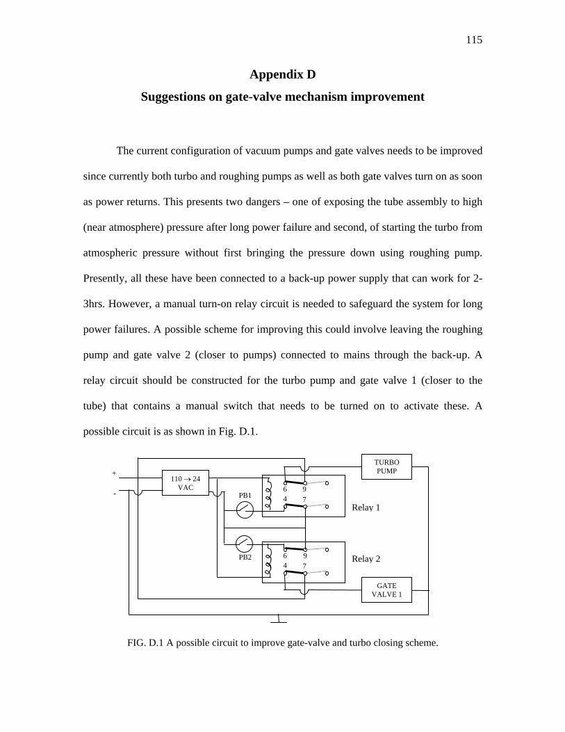
115
Appendix D
Suggestions on gate-valve mechanism improvement
The current configuration of vacuum pumps and gate valves needs to be improved
since currently both turbo and roughing pumps as well as both gate valves turn on as soon
as power returns. This presents two dangers – one of exposing the tube assembly to high
(near atmosphere) pressure after long power failure and second, of starting the turbo from
atmospheric pressure without first bringing the pressure down using roughing pump.
Presently, all these have been connected to a back-up power supply that can work for 2-
3hrs. However, a manual turn-on relay circuit is needed to safeguard the system for long
power failures. A possible scheme for improving this could involve leaving the roughing
pump and gate valve 2 (closer to pumps) connected to mains through the back-up. A
relay circuit should be constructed for the turbo pump and gate valve 1 (closer to the
tube) that contains a manual switch that needs to be turned on to activate these. A
possible circuit is as shown in Fig. D.1.
FIG. D.1 A possible circuit to improve gate-valve and turbo closing scheme.
110 → 24 VAC
TURBO PUMP
GATE VALVE 1
+
- 6 974
964 7
PB1
PB2
Relay 1
Relay 2

116
Under normal conditions, when power is present the two relays are closed i.e. for
each relay 9 is connected to 6 and 7 is connected to 4. Thus the electromagnets are
charged (getting ground through 7-4 connection and the gate valve 1 is closed and turbo
active through 9-6 connection. When power goes out, the electromagnets are no longer
charged and the relays open i.e. 6 and 4 are open (not connected to 9 and 7 respectively).
When power now returns, 4 is still not grounded through 7 and the two pushbuttons (PB1
and PB2) are open so the electromagnets are not charged. A manual push to the
pushbuttons is required to charge the electromagnets by providing the path to ground and
closing the relays again 9-6 and 7-4. Thus this circuit prevents gate valve 1 and turbo
pump from turning on as soon as power returns. The pushbutton can be used to manually
turn these on, first the turbo pump after ensuring that roughing pump has created pressure
~1 milliTorr and then gate valve 1 when the pressure is back to normal operating
conditions of 0.7-0.8x10⁻⁵.

117
Appendix E
Cathode Conditioning Procedure
If the TWT is not used for a long time, the cathode may need to be conditioned to
restore normal operation. If the cathode is not conditioned properly, the cathode current
keeps dropping and cannot be maintained at normal value. Conditioning involves heating
the cathode for long periods (6-7 hrs) to restore the cathode properties and correct beam
current.
Normal operation of the cathode is at ~1000° C temperature achieved with ~13 V
and 0.4 A. Starting with these values, keep the heater on for 2-3 hrs. Apply high voltage
to the cathode in pulses and watch beam current. If the current is still low, heater current
can be increased to 0.433 A (~1100° C) for a few (2-3) hrs maximum to push fresh
barium to the cathode surface. This should be done while pulsing the beam and
monitoring improvement in beam current. Also the system pressure should be monitored
to make sure that a lot of gas is not generated. The beam current should continue to
increase with time until the standard operating beam current is drawn from the cathode.
Now decreasing the filament current to normal operating value of 0.4 A should not
decrease the beam current, which should stay at the space charge limited value, if the
cathode has been conditioned.
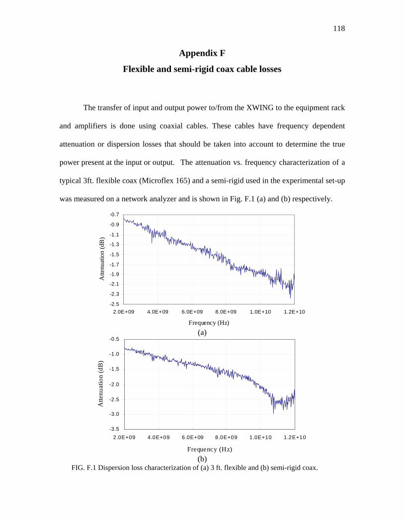
118
Appendix F
Flexible and semi-rigid coax cable losses
The transfer of input and output power to/from the XWING to the equipment rack
and amplifiers is done using coaxial cables. These cables have frequency dependent
attenuation or dispersion losses that should be taken into account to determine the true
power present at the input or output. The attenuation vs. frequency characterization of a
typical 3ft. flexible coax (Microflex 165) and a semi-rigid used in the experimental set-up
was measured on a network analyzer and is shown in Fig. F.1 (a) and (b) respectively.
-2.5
-2.3
-2.1
-1.9
-1.7
-1.5
-1.3
-1.1
-0.9
-0.7
2.0E+09 4.0E+09 6.0E+09 8.0E+09 1.0E+10 1.2E+10
Frequency (Hz)
Atte
nuat
ion
(dB
)
(a)
-3.5
-3.0
-2.5
-2.0
-1.5
-1.0
-0.5
2.0E+09 4.0E+09 6.0E+09 8.0E+09 1.0E+10 1.2E+10
Frequency (Hz)
Atte
nuat
ion
(dB
)
(b)
FIG. F.1 Dispersion loss characterization of (a) 3 ft. flexible and (b) semi-rigid coax.

119
Appendix G
Amplitude Correction Table for Output and Tap path
The frequency dependent losses in the output and tap path loss were characterized
and are shown in Table G.1. The output path includes the losses from the XWING output
to the output port on the switch control board assembly (Fig. 2.10) and includes output
semi-rigid, high power 20 dB attenuator, switching assembly and the semi-rigid S4
connecting the switch output to the control board. The tap path loss similarly includes tap
flexible cable from XWING, switching assembly and the semi-rigid from switch output
to control board. These losses are used to correct observed amplitude values.
Frequency
(GHz)
Output path loss
(dB)
Tap path loss
(dB)
0.5 21.2 1.3
1 21.7 1.8
2 22.6 2.6
3 23.3 3.3
4 24.0 3.8
5 24.5 4.4
6 25.3 5.0
7 25.6 5.3
8 26.3 5.9
9 26.8 6.5
10 27.8 7.2
11 27.4 7.3
12 28.2 7.3
TABLE G.1 Frequency dependent losses of output path and tap path.
120
REFERENCES
[1] The code can be obtained from http://www.lmsuite.org.
[2] C.S. Aitchison, M. Mbabele, M.R. Moazzam, D. Budimir and F. Ali,
“Improvement of Third-Order Intermodulation Product of RF and Microwave
Amplifiers by Injection”, IEEE Trans. on Microwave Theory and Techniques,
vol. 49, No. 6, pp. 1148-1154, June 2001.
[3] Aldo N. D’Andrea, V. Lottici and R. Reggiannini, “RF Power Amplifier
Linearization Through Amplitude and Phase Predistortion”, IEEE Trans. on
Comm., vol. 44, No. 11, pp. 1477-84, Nov. 1996.
[4] S. Bhattacharjee, C. Marchewka, J. Welter, R. Kowalczyk, C. B. Wilsen, Y. Y.
Lau, J. H. Booske, A. Singh, J. E. Scharer, R. M. Gilgenbach, M. J. Neumann,
and M. W. Keyser, “Suppression of third-order intermodulation in a klystron by
third-order injection”, Phys. Rev. Letter, 90, 2003. Article 098303.
[5] T. Chen, Y. Goren, C. Jensen, P. Lally and D. Gagne, “A Novel Technology for
Linearizing Traveling Wave Tube Amplifiers”, 2002 IEEE MTT-S International
Microwave Symposium Digest, vol. 2, pp. 773-776, 2002.
[6] A. Choffrut, B.D. Van Veen and J.H. Booske, “Traveling wave tube-based
LINC transmitters”, IEEE Trans. Electron Devices, vol. 50, No. 5, pp. 1405-07,
May 2003.
[7] M. Converse, “Investigation of the Mechanisms of Pulse Amplification in
Helical Traveling Wave Tubes”, PhD Thesis, University of Wisconsin –
Madison, 2003.
121
[8] D.C. Cox, “Linear Amplification with Nonlinear Components”, IEEE Trans. on
Comm., pp. 1942-45, Dec. 1974.
[9] N. J. Dionne, “Harmonic Generation in Octave Bandwidth Traveling-Wave
Tubes”, IEEE Trans. on Electron Devices, vol. 17, No. 4, pp. 365-372, April
1970.
[10] S.K. Dutta, P.K. Jain and B.N. Basu, “Control of IM3 distortion in helix TWTs
by harmonic injection – an Eulerian hydrodynamical study”, IEEE Trans.
Electron Devices, vol. 48, No. 1, pp. 62-66, 2001.
[11] S.K. Dutta, P.K. Jain, M.D. Rajnarayan and B.N. Basu, “Eulerian analysis for
harmonic generation in a helix travelling-wave tube”, Int. J. Electronics, vol. 85,
No. 3, pp. 377-395, 1998.
[12] Chun-Wah Fan, and K.M. Cheng, “Amplifier Linearization Using Simultaneous
Harmonic and Baseband Injection”, IEEE Microwaves and Wireless Comm.
Letters, vol. 11, No. 10, pp. 404-406, Oct. 2001.
[13] W.E. Garrigus and M.L. Glick, “Multi-octave high-power TWT operation”,
Microwave Journal, vol. 18, pp. 35-40, 1975.
[14] A.S. Gilmour, Jr., Principles of Traveling Wave Tubes, Artech House, Boston,
1994.
[15] J. J. Hamilton and D. Zavadil, “Harmonically-Enhanced Two-Octave TWTA”,
Microwave Journal, vol. 15, pp. 24-25, 1972.
[16] D.J. Jennings, A. Bateman and J.P. McGeehan, “Adjacent channel power and
error-vector magnitude performance of reduced complexity CALLUM
systems”, IEE Proc. Comm., vol 146, No. 5, pp. 297-302, Oct. 1999.
122
[17] Allen Katz, www.lintech.com/infodown.htm.
[18] J. T. Mendel, “Helix and Coupled-Cavity Traveling-Wave Tubes”, Proceedings
of the IEEE, vol. 61, No. 3, pp. 280-288, March 1973.
[19] B. Milovanovic, N. Males-Ilic and D. Budimir, “A multicarrier amplifier design
linearized through second harmonics and second-order IM feedback”, 5th
International Conference on Telecommunications in Modern Satellite, Cable
and Broadcasting Service, Nis, Yugoslavia, vol. 1, pp. 19-21, Sept.2001.
[20] M. Modeste, D. Budimir, M.R. Moazzam and C.S. Aitchison, “Analysis and
practical performance of a Difference frequency technique for improving the
multicarrier IMD performance of RF Amplifiers”, IEEE MTT-S Technol.
Wireless Applicant. Symp. Digest, Vancouver, BC, Canada, pp. 53-56, Feb.
1999.
[21] I. J. Morey and C. K. Birdsall, “Traveling-Wave-Tube Simulation: The IBC
Code”, IEEE Trans. Plasma Sci., vol. 18, No. 3, June 1990.
[22] J.R. Pierce, Traveling Wave Tubes, Van Nostrand, Princeton, N.J., 1950.
[23] J.G. Proakis, Digital Communications, McGraw-Hill, 4th edition, 2001.
[24] A.A.M. Saleh, “Frequency-independent and frequency-dependent nonlinear
models of TWT amplifiers”, IEEE Trans. Comm., COM-29, 11, pp. 1715-1720,
Nov. 1981.
[25] O. Sauseng, M.A. Huisjen and W.E. Garrigus, “Reduction of intermodulation
distortion with harmonic injection for wideband traveling-wave tubes”, IEDM
Technical Digest, pp. 411-414, 1975.
123
[26] A. Singh, J.G. Wöhlbier, J.H. Booske and J. E. Scharer, “Suppressing nonlinear
distortions in traveling-microwave tubes by harmonic injection”, Submitted to
Phys. Rev. Letters, 2003.
[27] M.A. Wirth, “Experimental Investigations of a Custom-made, Helical Traveling
Wave Tube Amplifier”, Master’s Thesis, University of Wisconsin – Madison,
2002.
[28] M.A. Wirth, A. Singh, J.E. Scharer and J.H. Booske, “Third-order
intermodulation reduction by harmonic injection in a TWT amplifier”, IEEE
Trans. Electron Devices, vol. 49, No. 6, pp. 1082-1084, 2002.
[29] J. G. Wöhlbier, “Nonlinear distortion and suppression in traveling wave tubes –
Insights and Methods”, PhD Thesis, University of Wisconsin – Madison, 2003.
[30] J. G. Wöhlbier and J.H. Booske, “Mechanisms for Phase Distortion in a
Traveling Wave Tube”, Submitted to Phys. Rev E, April 2003.
[31] J. G. Wöhlbier, J.H. Booske and I. Dobson, “On the Physics of Harmonic
Injection in a Traveling Wave Tube”, Submitted to IEEE Trans. Plasma Sci.,
May 2003.
[32] J. G. Wöhlbier, J.H. Booske and I. Dobson, “The Multifrequency Spectral
Eulerian (MUSE) model of a traveling wave tube”, IEEE Trans. Plasma Sci.,
vol. 30, No. 3, pp. 1063-1075, 2002.
[33] J. G. Wöhlbier, I. Dobson and J.H. Booske, “Generation and growth rates of
nonlinear distortions in a traveling wave tube”, Phys. Rev E, 66, 2002. Article
56504.