Research ArticleExperimental Investigation on Nonlinear Flow AnisotropyBehavior in Fracture Media

Chun Zhu ,1,2,3 Xiaoding Xu ,1,2 Xiuting Wang,3,4 Feng Xiong ,3,5 Zhigang Tao ,2

Yun Lin ,3,6 and Jing Chen2

1College of Construction Engineering, Jilin University, Changchun 130026, China2State Key Laboratory for Geomechanics & Deep Underground Engineering Beijing, China University of Mining & Technology,Beijing 100083, China3School of Civil, Environmental and Mining Engineering, The University of Adelaide, Adelaide, SA 5005, Australia4School of Civil Engineering and Architecture, Anhui University of Science and Technology, Huainan 232000, China5School of Civil Engineering, Wuhan University, Hubei 430072, China6School of Resource and Safety Engineering, Central South University, Changsha, Hunan 410083, China

Correspondence should be addressed to Feng Xiong; whufengx@163.com and Zhigang Tao; zhigangtao_cumtb@126.com

Received 26 February 2019; Accepted 9 June 2019; Published 24 June 2019

Guest Editor: Frédéric Nguyen

Copyright © 2019 Chun Zhu et al. This is an open access article distributed under the Creative Commons Attribution License,which permits unrestricted use, distribution, and reproduction in any medium, provided the original work is properly cited.

A series of flow experiments were performed on matched fractures to study the problem of non-Darcy flow in fractured media. Fiverock fractures of different roughness were generated using indirect tensile tests, and their surface topographies were measured usinga stereo topometric scanning system. The fracture was assumed to be a self-affine surface, and its roughness and anisotropy werequantified by the fractal dimension. According to the flow tortuosity effect, the nonlinear flow was characterized by hydraulictortuosity and surface tortuosity power law relationships based on Forchheimer’s law. Fracture seepage experiments conductedwith two injection directions (0° and 90°) showed that Forchheimer’s law described the nonlinear flow well. Both the proposedmodel and Chen’s double-parameter model gave similar results to the experiment, but the match was closer with the proposedmodel. On this basis, a new formula for the critical Reynolds number is proposed, which serves to distinguish linear flow andForchheimer flow.

1. Introduction

A long history of geological and human activities has causedmost rock masses to be cut by a large number of faults andfractures [1–5]. These discontinuities form the main chan-nels for groundwater flow, which control the permeabilitycharacteristics of the rock mass. In the study of rock masshydrology, discontinuities are usually generalized into twosmooth parallel plates, and the famous cubic law is henceobtained through theory and experiment. A variety of correc-tion models [6–11] has been proposed to account for fractureroughness, contact, or filling.

Some engineering projects involve a high hydraulic gra-dient, for example, dam construction in the deep weak over-burden of a river valley, exploitation of low-permeability oil

and gas wells, and coal mine gas outbursts [12–16]. Underthis condition, fluid flow through fractures is not linear,and the use of the cubic law or related modified modelswould cause large deviations. The well-known Forchheimerlaw is used to describe this flow behavior:

∇P = AQ + BQ2, 1

where ∇P is the pressure gradient between the inlet and out-let of the fracture, Q is the flow rate through the fracture, andA and B are the coefficients of viscosity and inertia, respec-tively. Zimmerman et al. [17] observed the Forchheimer flowphenomena of rough fractures when the Reynolds numberRe > 20 through experiments and numerical methods. Zhangand Nemcik [18] discussed the linear and nonlinear flow

HindawiGeofluidsVolume 2019, Article ID 5874849, 9 pageshttps://doi.org/10.1155/2019/5874849

characteristics of rough fractures under different confiningpressures. Zhou et al. [19] explained the physical significanceof the Forchheimer flow coefficients A and B and the internaltransition mechanism on the basis of water pressure testsunder different confining pressures. However, the effects offracture roughness on flow were not explained in detail. Jinet al. (2013) pointed out that the influence of a rough geom-etry on fracture flow is manifested in three aspects: the fric-tional effect in the fluid, the tortuous effect of the fracturesurface, and a local roughness effect. Tsang [20] consideredthat the roughness of the fracture surface would lead to flowtortuosity, and Xiao et al. [21] introduced a tortuosity factorto describe the tortuosity of flow. Watanabe et al. [22] carriedout fluid flow experiments in fractures with shear displace-ments and found that the nonlinear flow effect decreases asshear increases.

Fractal geometrywasfirst put forwardbyB.B.Mandelbrot.Xie and Wang [23] introduced it into the description offracture roughness and then used it to describe fluid flowcharacteristics at rock fracture surfaces. Murata and Saito[24] studied the influence of fractal parameters on the tortu-osity effect, and Wang et al. [25] put forward a flow modelusing fractal parameters. Ju et al. [26] carried out flow exper-iments on rough single fractures with different fractaldimensions. These flow tests clarified the influence of arough structure on seepage flow. Develi and Babadagli [27]carried out saturated seepage tests on seven kinds of artifi-cial tensional fracture surfaces, describing the roughness ofthe fractures by means of the fractal dimension and discuss-ing the influences of roughness, anisotropy, and normalstress on seepage characteristics.

In this paper, a nonlinear fractal model for rough frac-tures is deduced based on the tortuous effect and the self-affine fractal characteristics of the fracture surface. The lawand anisotropy of Forchheimer flow are analyzed, and thenew model is verified by seepage tests.

2. Nonlinear Fractal Model for Rough-WalledRock Fractures

Forchheimer’s law is composed of a linear part AQ and anonlinear part BQ2. When the flow rate is low, a cubic lawcan be used to describe the relationship of the flow rate andpressure. Hence, A can be expressed as

A = 12μwe3h

, 2

where μ is the dynamic coefficient of viscosity of the fluid andw is the width of the fracture. eh is the hydraulic aperture,which can be calculated as eh = 12μQ/w/▽P 1/3.

The coefficient B represents the degree that the seep-age curve deviates from that in the linear stage. Schraufand Evans [28] put forward a form of B using dimen-sional analysis:

B = bDρ

e3hw2 , 3

where ρ is the fluid density and bD is a parameter relatedto the roughness of the fracture surface. Chen et al. [6]used the peak asperity height to describe fracture rough-ness and obtained a two-parameter model for bD:

bD = aξ

2eh

b

, 4

where a and b are fitting parameters, respectively. How-ever, the peak asperity height does not account for flowtortuosity and anisotropy. Chen et al. [6] also usednumerical simulation to study non-Darcy behavior in frac-ture flow. The results showed that the rougher the surfacewas, the more tortuous the flow would be, and eddy cur-rents and recirculation would occur at high velocity,which would increase the inertial resistance. In order tocharacterize the effect of flow tortuosity, the followingpower law relations are proposed by Murata and Saito[24] and Ji et al. (2015):

bD = cτaτbs , 5

where a, b, and c are fitting parameters. τ is the hydrolog-ical curvature, which is defined as the ratio of the actuallength Lt of the seepage path to the horizontal length Lcalong the pressure gradient of the fracture. τs is the curva-ture of the surface, which is defined as the ratio of thesurface area to the projection area of the fracture surface.

For fractal fractures, the relationship between measureF δ and measurement scale δ is as follows:

F δ = F0δα, 6

where α is a parameter related to the fractal dimension D andD is in the range 1-3. F0 is the apparent measurement. Basedon this, the relationship between the fracture surface area Asand a square mesh with dimension δ1 is as follows:

As = F1δ2−Ds1 , 7

where Ds is the fractal dimension of the fracture area. For asquare fracture, when δ1 is equal to Lc and equation (7) issubstituted into As Lc = Ac, F1 can be obtained as follows:

F1 = AcDs/2 8

Hence, τs can be obtained:

τs =As δ1Ac

= δ21Ac

2−Ds

9

In addition, the fractal relationship of the length of theseepage path Lt and measure δ2 is as follows:

Lt δ2 = F2δ1−DT2 , 10

2 Geofluids

where DT is the fractal dimension of the seepage path.When δ2 is equal to Lc and equation (10) is substituted intoLt Lc = Lc, F2 can be obtained as

F2 = LDTc 11

Hence, τ can be obtained:

τ = Lt δ2Lc

= δ2Lc

1−DT

12

Mandelbrot, the founder of fractal theory, suggestedthat the fractal dimension of the surface could be calcu-lated by adding the dimension of a surface profile to 1.Therefore, the relationship between the fractal dimensionof the profile length and the fractal dimension of the areais as follows:

Ds =Dl + 1 13

Jin et al. [29] considered Dl as equal to DT . Hence, bDcan be obtained by substituting equation (9) and equation(12) into equation (5):

bD = cδ2Lc

a 1−Dl δ21Ac

b 1−Dl

14

When δ1 and δ2 are eh, equation (1) becomes

bD = cehLc

a+b 1−Dl

15

Hence, a new model of parameter B in Forchheimer’slaw can be obtained:

B = aehLc

b 1−Dl ρ

e3hw2 , 16

where a and b are constants that can be determined withfracture permeability tests. Firstly, the fractal dimension iscalculated from fracture surface data. The curve relatingflow to pressure gradient is then obtained through fracturepermeability tests, and this is used to obtain a and b.

3. Fracture Surface Measurement

3.1. Rock Fracture Preparation. The effect of fracture surfaceroughness on fluid flow was studied by way of saturated seep-age tests of rock fracture surfaces of different roughness. Anatural fracture surface is difficult to obtain, so artificial ten-sion fracture specimens were used to study the characteristicsof fluid flow in fractures. In this study, natural graniteselected from a quarry in Sichuan Province was processedinto 150mm × 150mm × 150mm square specimens in thelaboratory, and then, the specimens were split using theBrazilian splitting test method to obtain artificial tensional

joint specimens. Finally, five groups of fracture surfaces (F1,F2, F3, F4, and F5) with different roughness were prepared.

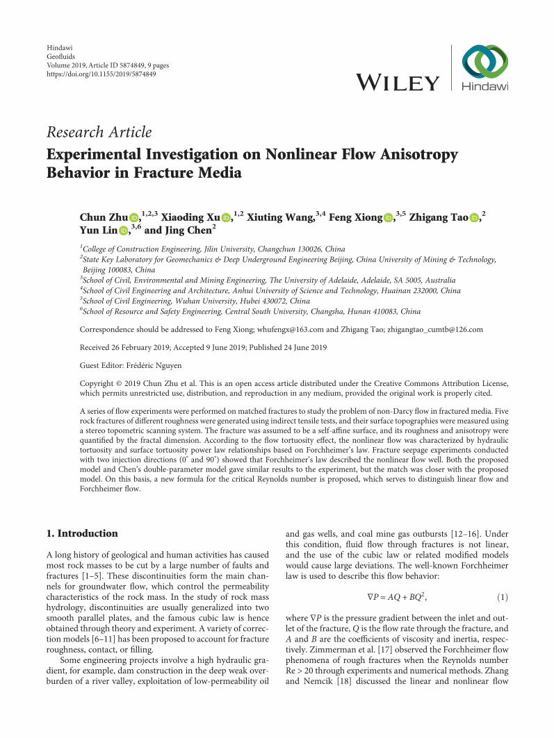
3.2. Measurement Procedure. A portable 3D optical three-dimensional scanning system was used to measure thethree-dimensional morphology of the fracture surface(Figure 1). The system broadly comprises a scanning controlunit, scanning lens, turn table, and tripod. The scanning lensis placed on the tripod, which can rotate freely and adjust itsposition conveniently. The other components are connectedvia USB. The system acquires a visible grating image pro-jected onto the surface of the object then accurately deter-mines the spatial coordinates (X, Y , Z) of each point usingthe phase and triangulation methods according to the shapeof fringe curvature change, forming a three-dimensionalpoint cloud data. This approach has the benefits of beingfast, high precision (measuring accuracy 25 μm), and allow-ing noncontact measurement.

In the actual measurement process, features of the mea-surement environment (light, dust, etc.) and the measure-ment methods will have an impact on the accuracy of thethree-dimensional topographic data. Therefore, after acquir-ing the three-dimensional data for a fracture surface, thepoint cloud data were processed by using the self-containedsoftware CloudForm to reduce noise, remove irrelevantpoints, filter data ripples, and patch. Additionally, theoriginal point cloud of the fracture surface is composed ofhundreds of thousands of discrete points with an averagespacing of 0.025mm, which amount to a huge amount of dis-ordered data. Data analysis was facilitated by compiling theprogram with MATLAB software to delete and reorder themeasured points. The newly obtained fracture surface has atotal of 22801 points at an average spacing of 1mm. Themeasured topographic parameters of the fracture surfacesshown in Figure 2 are listed in Table 1.

4. Calculation of Fractal Dimension

There are many methods for calculating the fractal dimen-sion of a rough fracture surface. Clarke [30] first proposed

Fracture specimen

Rotary table

Figure 1: Stereo topometric scanning system.

3Geofluids

0 20 40 60 80 100 120 1400

20

40

60

80

100

120

140

x (mm)

y (m

m)

9.750

11.76

13.76

15.77

17.77

19.78

21.79

23.79

25.80

z (mm)

(a) F1

0 20 40 60 80 100 120 1400

20

40

60

80

100

120

140

y (m

m)

x (mm)

z (mm)

3.550

5.269

6.988

8.706

10.43

12.14

13.86

15.58

17.30

(b) F2

0 20 40 60 80 100 120 1400

20

40

60

80

100

120

140

y (m

m)

x (mm)

z (mm)

6.900

9.281

11.66

14.04

16.43

18.81

21.19

23.57

25.95

(c) F3

0 20 40 60 80 100 120 1400

20

40

60

80

100

120

140

y (m

m)

x (mm)

z (mm)

6.100

7.619

9.137

10.66

12.18

13.69

15.21

16.73

18.25

(d) F4

0 20 40 60 80 100 120 1400

20

40

60

80

100

120

140

z (mm)

y (m

m)

x (mm)

5.700

8.400

11.10

13.80

16.50

19.20

21.90

24.60

27.30

(e) F5

Figure 2: Surfaces topographies of fractures (lower surfaces).

Table 1: Geometrical details of fractures.

Specimen Length L (mm) Width w (mm) Peak asperity height ξ (mm) Variance Rrms (mm2) Average Rm (mm) JRC

F1 149.9 150.1 3.74 2.06 1.58 11.3

F2 150.1 150.0 3.65 2.07 1.55 11.0

F3 150.1 150.1 3.97 4.14 3.52 12.8

F4 150.2 149.9 4.89 5.16 4.39 16.9

F5 150.1 149.9 3.27 3.87 3.29 13.9

4 Geofluids

the triangular prism surface area method, which takes thespatial surface area as the variable and a square grid asthe measure scale. Later, Xie and Wang [23] proposed aprojection coverage method. These two methods can be cat-egorized as driver methods. The dimension calculated bythese two methods is a similar fractal dimension, not a geo-metric fractal dimension. Zhou et al. [19] proposed box-counting methods for calculating the fractal dimension of athree-dimensional surface, including a cube coverage methodand an improved cube coverage method. The above compu-tational theories are based on statistical self-similarity. How-ever, Brown [31] and Kulatilake et al. [32, 33] argue thatrough rock fracture surfaces conform to the characteristicsof a self-affine model.

Kulatilake et al. [32] put forward a variogram methodas a self-affine model to determine the fractal dimension.This takes the variogram function 2γ x, h of the profile asa variable and the interval distance h as the measure scale.

The detailed method is as follows:

Step 1.Generation of two-dimensional contour data in differ-ent directions. Firstly, the fracture surface data are meshedinto 1mm × 1mm grids. 2D profiles are divided from thefracture surface data in accordance with the directions θ =15 × k k = 1, 2,⋯, 11 . The height data Z x, y of a direc-tional line is then calculated. The height data ZQ of the coor-dinate Q x, y is found on the 15-degree directional line P.The height of the coordinate radius within a 1mm range iscalculated according to equation (17). The profile data arethen obtained cyclically. The next set of profile data with adistance of 10mm is obtained by the same method. Finally,the profile data in each direction are obtained by repeatedcyclic calculation.

Z x, y = ∑ni=1Zi/ri

∑ni=11/ri

, 17

where Zi is the height of the point within a radius of1mm from point Q and ri is the distance from point i topoint Q.

Step 2. Calculation of the fractal dimension of all of the direc-tional lines. The variogram function is defined as

2γ h = 1N〠N

i=1Zi+1 − Zi

2, 18

where γ h L2 is the semivariogram, Zi L and Zi+1 Lare the heights of the 2D profile from the baseline, andN is the number of pairs of Z at a lag distance hbetween them. γ h can be simplified as a power-law func-tion in the self-affine profile as h→ 0:

2γ h = Kvh2H , 19

where Kv is a proportionality constant and H is the Hurstexponent, which is related to the fractal dimension by Dv =

2 −H. However, equation (18) and equation (19) cannot beused to calculate Dv directly. Dv should be written in the log-arithmic form

log 2γ h = 2 2 −Dv log h + log Kv , 20

so that Dv can be obtained by linear regression analysis. Atleast seven variance functions at different intervals h arecalculated for each profile line, and fractal dimension D isobtained by fitting equation (20). The fractal dimension Dof all of the profiles in one direction is averaged, and thefractal dimension D in that direction is obtained.

To make the anisotropic characteristics of fracture sur-face roughness more intuitive, Table 2 presents rose dia-grams of the fractal dimensions of five different fracturesurfaces (F1–F5). The fractal dimension is randomly distrib-uted in all directions, and the fracture surfaces are charac-terized by an irregular anisotropic roughness structure.The fractal dimension of the fracture surface of F4 is largerthan that of the others and is the highest, 1.60, in the 90°

direction. Therefore, F4 has the greatest roughness of thefracture surfaces.

It is noted that the fractal dimension D does not take thedifference between forward and backward on the 2D profileinto consideration. For example, the fractal dimension ofthe 0° profile is the same as that of 180°. Hence, equation(20) is correct when assuming there is the same nonlinearflow in the θ and θ + 180° directions.

5. Nonlinear Flow Behavior of Rough-WalledRock Fractures

5.1. Seepage Tests of Rough-Walled Rock Fractures. The fivegroups of rock fracture surfaces (F1–F5) mentioned in theprevious section were prepared for flow testing with a self-designed device. A detailed description of the device is givenin Xiong et al. [7]. Two flow directions (0° and 90°) weretested for each group of fractures, as shown in Figure 3.The pressure difference P under different flow rates Q wasrecorded during the test process; flow rates were in the range0–100ml/s during the tests.

5.2. Nonlinear Flow Behavior. Figures 4 and 5 show the rela-tionship between the flow rate Q and the pressure gradient∇P of each fracture in the 0° and 90° directions. When theflow rate is small (Q < 10ml/s), the pressure gradientincreases linearly with the flow rate. When the flow rateincreases, the pressure gradient increases nonlinearly, show-ing an increase in the inertia effect. In order to describe thisrelationship, the Forchheimer formula was used to fit the testdata for the 0° and 90° directions. The fitting results areshown in Table 3. These results indicate that Forchheimer’slaw (equation (1)) is able to quantitatively describe the non-linear flow behavior, which is consistent with Zimmermanet al. [17].

In order to analyze the anisotropic characteristics of flowin a rock fracture, a new parameter describing anisotropy is

5Geofluids

proposed: the ratio of the difference between the 90° and 0°

pressure gradients and the 90° pressure gradient.

anisotropy = ∇P90°−∇P0°∇P90°

, 21

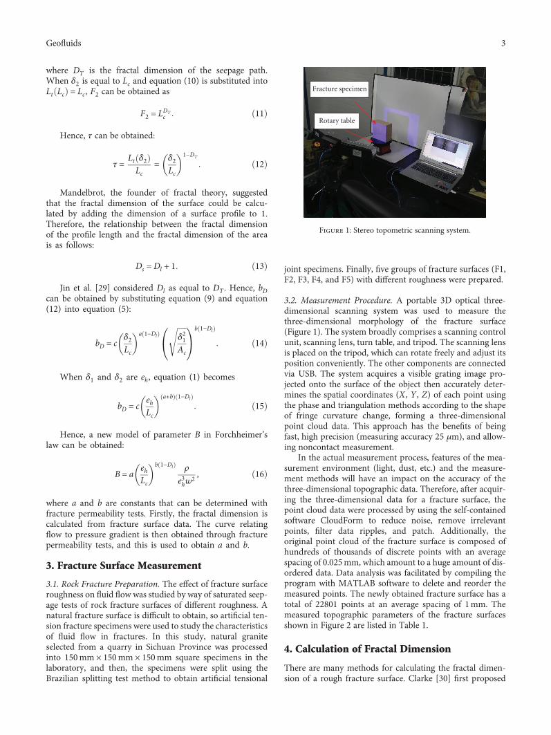
where ∇P90° is the pressure gradient in the 90° direction and∇P0° is the pressure gradient in the 0° direction. Figure 6shows the variation of anisotropy with flow rate. The anisot-

ropy values differ between the different groups, which indi-cate that the anisotropy of fracture flow exists and is relatedto the fracture morphology and aperture distribution.

Normalized transmissivity (Ta/T0) is determined byZimmerman et al. [17] in the following form:

Ta

T0= 11 + β Re , 22

where Ta is the apparent transmissivity and T0 is a specialapparent transmissivity in Darcy’s flow state and is typicallycalled intrinsic transmissivity. According to experimentaldata, the values of β are listed in Table 2. The relationshipof bD and β is plotted in Figure 7. It can be seen from the fig-ure that as bD increases, β linearly increases. And β is about12 times than bD, which is consistent with Zimmermanet al. [17].

5.3. Verification of the Nonlinear Flow Model Based onFractal Theory. In order to solve the undetermined constantsa and b, fracture morphology data were first obtained for F1,F2, and F3, and the fractal dimension was then calculatedaccording to the method detailed in Section 4. Then, theseepage test results were fitted according to the Levenberg-Marquardt method, and the parameters a and b were foundto be 0.246 and -0.964, respectively.

In order to verify the model, the nonlinear fractal modelis compared with the seepage test data and Chen’s two-parameter model [6].

For fractures F4 and F5, pressure gradients were calcu-lated according to the proposed model and the Chen model,respectively, and the results were compared with the experi-mental values, as shown in Figure 8. It can be seen that theresults calculated with the nonlinear fractal model are closeto the measured values, and the relative errors are mostlywithin 20%. This shows that the nonlinear fractal model givesa better description of nonlinear seepage in fractured media

Table 2: The fractal dimensions at different directions.

Directions (°) F_1 F_2 F_3 F_4 F_5

0 1.422 1.497 1.421 1.418 1.475

30 1.398 1.486 1.391 1.426 1.426

60 1.431 1.477 1.417 1.486 1.435

90 1.542 1.503 1.434 1.600 1.436

120 1.478 1.466 1.471 1.489 1.389

150 1.425 1.459 1.370 1.424 1.407

180 1.422 1.497 1.421 1.418 1.475

210 1.398 1.486 1.391 1.426 1.426

240 1.431 1.477 1.417 1.486 1.435

270 1.542 1.503 1.434 1.600 1.436

300 1.478 1.466 1.471 1.489 1.389

330 1.425 1.459 1.370 1.424 1.407

Lower specimen

Upper specimen

Flow direction (0º)

Flow direction (90º)

Figure 3: Different directions of flow (0° and 90°) in a rock fracture.

0 10 20 30 40 50 60 70 80 90 100 1100

1500

3000

4500

6000

7500

9000

10500

▽P

(Pa/

m)

Q (mm3/s)F1F2F3

F4F5

Figure 4: Relationship between pressure gradient and flowrate inthe 0° direction.

▽P

(Pa/

m)

0 20 40 60 80 1000

1500

3000

4500

6000

7500

Q (mm3/s)

F1F2F3

F4F5

Figure 5: Relationship between pressure gradient and flowrate inthe 90° direction.

6 Geofluids

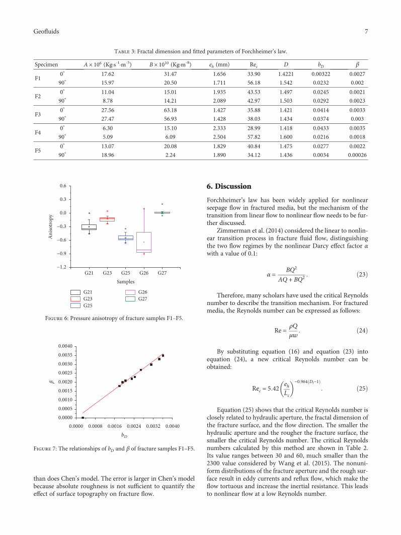
than does Chen’s model. The error is larger in Chen’s modelbecause absolute roughness is not sufficient to quantify theeffect of surface topography on fracture flow.

6. Discussion

Forchheimer’s law has been widely applied for nonlinearseepage flow in fractured media, but the mechanism of thetransition from linear flow to nonlinear flow needs to be fur-ther discussed.

Zimmerman et al. (2014) considered the linear to nonlin-ear transition process in fracture fluid flow, distinguishingthe two flow regimes by the nonlinear Darcy effect factor αwith a value of 0.1:

α = BQ2

AQ + BQ2 23

Therefore, many scholars have used the critical Reynoldsnumber to describe the transition mechanism. For fracturedmedia, the Reynolds number can be expressed as follows:

Re = ρQμw

24

By substituting equation (16) and equation (23) intoequation (24), a new critical Reynolds number can beobtained:

Rec = 5 42 ehLc

−0 964 Dl−125

Equation (25) shows that the critical Reynolds number isclosely related to hydraulic aperture, the fractal dimension ofthe fracture surface, and the flow direction. The smaller thehydraulic aperture and the rougher the fracture surface, thesmaller the critical Reynolds number. The critical Reynoldsnumbers calculated by this method are shown in Table 2.Its value ranges between 30 and 60, much smaller than the2300 value considered by Wang et al. (2015). The nonuni-form distributions of the fracture aperture and the rough sur-face result in eddy currents and reflux flow, which make theflow tortuous and increase the inertial resistance. This leadsto nonlinear flow at a low Reynolds number.

Table 3: Fractal dimension and fitted parameters of Forchheimer’s law.

Specimen A × 106 (Kg·s-1·m-5) B × 1010 (Kg·m-8) eh (mm) Rec D bD β

F10° 17.62 31.47 1.656 33.90 1.4221 0.00322 0.0027

90° 15.97 20.50 1.711 56.18 1.542 0.0232 0.002

F20° 11.04 15.01 1.935 43.53 1.497 0.0245 0.0021

90° 8.78 14.21 2.089 42.97 1.503 0.0292 0.0023

F30° 27.56 63.18 1.427 35.88 1.421 0.0414 0.0033

90° 27.47 56.93 1.428 38.03 1.434 0.0374 0.003

F40° 6.30 15.10 2.333 28.99 1.418 0.0433 0.0035

90° 5.09 6.09 2.504 57.82 1.600 0.0216 0.0018

F50° 13.07 20.08 1.829 40.84 1.475 0.0277 0.0022

90° 18.96 2.24 1.890 34.12 1.436 0.0034 0.00026

G21 G23 G25 G26 G27−1.2

−0.9

−0.6

−0.3

0.0

0.3

0.6

Ani

sotr

opy

G21G23G25

G26G27

Samples

Figure 6: Pressure anisotropy of fracture samples F1–F5.

0.0000 0.0008 0.0016 0.0024 0.0032 0.00400.00000.00050.00100.0015

𝛽 0.00200.00250.00300.00350.0040

bD

Figure 7: The relationships of bD and β of fracture samples F1–F5.

7Geofluids

7. Conclusions

This paper discusses the effect of roughness on nonlinearflow in a rock fracture based on previous research and anal-ysis of physical laboratory experiments. The main conclu-sions are as follows:

(1) A new nonlinear seepage model for rough fractures,equation (16), is proposed according to flow tortuos-ity in the fracture and the fractal characteristics of thefracture

(2) The 3D optical three-dimensional scanning systemwas used to acquire point cloud data from fracturesurfaces. The self-affine fractal dimension calculationmethod proposed by Kulatilake et al. [32] was used toanalyze the anisotropic characteristics of the rough-ness of the fracture surface

(3) Five different kinds of rough fractures were tested inseepage experiments in the 0° and 90° directions. Theresults show that fracture flow conforms to Forchhei-mer’s law and has clear isotropic characteristics. Thenew model generates results that are closer to thosefrom the experiment than does Chen’s two-parameter model

(4) According to the new model, a new expression of thecritical Reynolds number (equation (25)) for distin-guishing Darcy flow from Forchheimer flow is pro-posed. It shows that the critical Reynolds number isclosely related to hydraulic aperture, the roughnessof the fracture surface, and the flow direction

Data Availability

The data are all available and have been explained in thisarticle; readers can access the data supporting the conclusionsof the study.

Conflicts of Interest

The authors declare that they have no conflicts of interest

Authors’ Contributions

Chun Zhu and Yun Lin contributed equally to this work.

Acknowledgments

This work was supported by the Key Research and Develop-ment Project of Zhejiang Province (Grant No. 2019C03104)and the Special Funds of Fundamental Research Funds forCentral Universities (2015QB02). The first author is gratefulto the Chinese Scholarship Council and the University ofAdelaide for providing an opportunity to conduct thisresearch as a joint Ph.D. student.

References

[1] W. P. Huang, C. Li, L. W. Zhang, Q. Yuan, Y. S. Zheng, andY. Liu, “In situ identification of water-permeable fracturedzone in overlying composite strata,” International Journal ofRock Mechanics and Mining Sciences, vol. 105, pp. 85–97,2018.

[2] Y. Li, S. Zhang, and X. Zhang, “Classification and fractal char-acteristics of coal rock fragments under uniaxial cyclic loadingconditions,” Arabian Journal of Geosciences, vol. 11, no. 9,p. 201, 2018.

[3] X.Wang and L. Tian, “Mechanical and crack evolution charac-teristics of coal–rock under different fracture-hole conditions:a numerical study based on particle flow code,” EnvironmentalEarth Sciences, vol. 77, no. 8, p. 297, 2018.

[4] Z. Wu, H. Sun, and L. N. Y. Wong, “A cohesive element-basednumerical manifold method for hydraulic fracturing model-ling with voronoi grains,” Rock Mechanics and Rock Engineer-ing, pp. 1–25, 2019.

[5] S. C. Zhang, Y. Y. Li, B. T. Shen, X. Sun, and L. Gao, “Effectiveevaluation of pressure relief drilling for reducing rock bursts

0 20 40 60 80 1000

300600900

120015001800210024002700

▽P

(Pa/

m)

Q (mm3/s)Experiment ExperimentProposed model Proposed modelChen model Chen model

(a) F4

0 20 40 60 80 1000

500

1000

1500

2000

2500

3000

3500

4000

▽P

(Pa/

m)

Q (mm3/s)

Experiment ExperimentProposed model Proposed modelChen model Chen model

(b) F5

Figure 8: Comparison of results from equation (21), equation (22), and experimental measurements (open point is flow test along the0° direction and solid point is flow test along the 90° direction; dashed line and solid line are proposed and the Chen model in 0° and90° directions, respectively).

8 Geofluids

and its application in underground coal mines,” InternationalJournal of Rock Mechanics and Mining Sciences, vol. 114,pp. 7–16, 2019.

[6] Y. F. Chen, J. Q. Zhou, S. H. Hu, R. Hu, and C. B. Zhou, “Eval-uation of Forchheimer equation coefficients for non-Darcyflow in deformable rough-walled fractures,” Journal of Hydrol-ogy, vol. 529, pp. 993–1006, 2015.

[7] F. Xiong, Q. Jiang, Z. Ye, and X. Zhang, “Nonlinear flowbehavior through rough-walled rock fractures: the effect ofcontact area,” Computers and Geotechnics, vol. 102, pp. 179–195, 2018.

[8] F. Xiong, Q. Jiang, C. Xu, X. Zhang, and Q. Zhang, “Influencesof connectivity and conductivity on nonlinear flow behavioursthrough three-dimension discrete fracture networks,” Com-puters and Geotechnics, vol. 107, pp. 128–141, 2019.

[9] C. Yao, C. He, J. Yang, Q. Jiang, J. Huang, and C. Zhou, “Anovel numerical model for fluid flow in 3D fractured porousmedia based on an equivalent matrix-fracture network,” Geo-fluids, vol. 2019, Article ID 9736729, 13 pages, 2019.

[10] Z. Ye, Q. Jiang, C. Yao et al., “The parabolic variationalinequalities for variably saturated water flow in heterogeneousfracture networks,” Geofluids, vol. 2018, Article ID 9062569,16 pages, 2018.

[11] R. W. Zimmerman and G. S. Bodvarsson, “Hydraulic conduc-tivity of rock fractures,” Transport in Porous Media, vol. 23,no. 1, pp. 1–30, 1996.

[12] S. Gentier, D. Hopkins, and J. Riss, “Role of fracture geometryin the evolution of flow paths under stress,” in Dynamics ofFluids in the Fractured Rock, pp. 169–184, American Geophys-ical Union, 2000.

[13] T. Ishibashi, N. Watanabe, N. Hirano, A. Okamoto, andN. Tsuchiya, “Beyond-laboratory-scale prediction for channel-ing flows through subsurface rock fractures with heterogeneousaperture distributions revealed by laboratory evaluation,” Jour-nal of Geophysical Research: Solid earth, vol. 120, no. 1, pp. 106–124, 2014.

[14] Q. Jiang and C. Zhou, “A rigorous solution for the stability ofpolyhedral rock blocks,” Computers and Geotechnics, vol. 90,pp. 190–201, 2017.

[15] T. Zhigang, Z. Chun, W. Yong, W. Jiamin, H. Manchao,and Z. Bo, “Research on stability of an open-pit mine dumpwith fiber optic monitoring,” Geofluids, vol. 2018, Article ID9631706, 20 pages, 2018.

[16] P. A. Witherspoon, “Investigation at Berkeley on fractureflow in rocks: from the parallel plate model to chaotic systems,”in Dynamics of Fluid in Fractured Rocks, B. Faybishenko, S.Benson, and P. Witherspoon, Eds., pp. 1–58, American Geo-physical Union, Washington, DC, USA, 2000.

[17] R. W. Zimmerman, A. al-Yaarubi, C. C. Pain, and C. A.Grattoni, “Nonlinear regimes of fluid flow in rock frac-tures,” International Journal of Rock Mechanics and MiningSciences, vol. 41, no. 3, pp. 163–169, 2004.

[18] Z. Zhang and J. Nemcik, “Fluid flow regimes and nonlinearflow characteristics in deformable rock fractures,” Journal ofHydrology, vol. 477, no. 1, pp. 139–151, 2013.

[19] J.-Q. Zhou, S.-H. Hu, S. Fang, Y.-F. Chen, and C.-B. Zhou,“Nonlinear flow behavior at low Reynolds numbers throughrough-walled fractures subjected to normal compressive load-ing,” International Journal of Rock Mechanics and Mining Sci-ences, vol. 80, pp. 202–218, 2015.

[20] Y. W. Tsang, “The effect of tortuosity on fluid flow through asingle fracture,” Water Resources Research, vol. 20, no. 9,pp. 1209–1215, 1984.

[21] W. Xiao, C. Xia, W. Wang, and Y. Bian, “Study on calculationof fluid flow through a single rough joint by considering flowtortuosity effect,” Chinese Journal of Rock Mechanics and Engi-neering, vol. 30, no. 9, pp. 2416–2425, 2011.

[22] N. Watanabe, N. Hirano, and N. Tsuchiya, “Diversity ofchanneling flow in heterogeneous aperture distributioninferred from integrated experimental‐numerical analysis onflow through shear fracture in granite,” Journal of GeophysicalResearch, vol. 114, pp. 115–123, 2009.

[23] H. Xie and J. Wang, “Direct fractal measurement of fracturesurfaces,” International Journal of Solids and Structures,vol. 36, no. 20, pp. 3073–3084, 1999.

[24] S. Murata and T. Saito, “Estimation of tortuosity of fluid flowthrough a single fracture,” Journal of Canadian PetroleumTechnology, vol. 42, no. 12, pp. 39–45, 2003.

[25] G. Wang, N. Huang, Y. Jiang, B. Li, W. Xuezhen, andX. Zhang, “Seepage calculation model for rough joint surfaceconsidering fracture characteristics,” Chinese Journal of RockMechanics and Engineering, vol. 33, pp. 3397–3405, 2014.

[26] Y. Ju, Q. G. Zhang, Y. M. Yang, H. P. Xie, F. Gao, and H. J.Wang, “An experimental investigation on the mechanism offluid flow through single rough fracture of rock,” Science ChinaTechnological Sciences, vol. 56, no. 8, pp. 2070–2080, 2013.

[27] K. Develi and T. Babadagli, “Experimental and visual analysisof single-phase flow through rough fracture replicas,” Interna-tional Journal of Rock Mechanics and Mining Sciences, vol. 73,pp. 139–155, 2015.

[28] T. W. Schrauf and D. D. Evans, “Laboratory studies of gas flowthrough a single natural fracture,” Water Resources Research,vol. 22, no. 7, pp. 1038–1050, 1986.

[29] Y. Jin, J. L. Zheng, J. B. Dong, C. H. Huang, X. Li, and Y. Wu,“Fractal seepage law characterizing fluid flow through a singlerough cleat composed of self-affine surfaces,” Chinese ScienceBulletin, vol. 60, no. 21, pp. 2036–2047, 2015.

[30] K. C. Clarke, “Computation of the fractal dimension of topo-graphic surfaces using the triangular prism surface areamethod,” Computers and Geosciences, vol. 12, no. 5, pp. 713–722, 1986.

[31] S. R. Brown, “Fluid flow through rock joints: the effect of sur-face roughness,” Journal of Geophysical Research: Solid Earth,vol. 92, no. B2, pp. 1337–1347, 1987.

[32] P. H. S. W. Kulatilake, P. Balasingam, J. Park, and R. Morgan,“Natural rock joint roughness quantification through fractaltechniques,” Geotechnical and Geological Engineering, vol. 24,no. 5, pp. 1181–1202, 2006.

[33] P. H. S. W. Kulatilake, J. Park, P. Balasingam, and R. Morgan,“Quantification of aperture and relations between aperture,normal stress and fluid flow for natural single rock fractures,”Geotechnical and Geological Engineering, vol. 26, no. 3,pp. 269–281, 2008.

9Geofluids

Hindawiwww.hindawi.com Volume 2018

Journal of

ChemistryArchaeaHindawiwww.hindawi.com Volume 2018

Marine BiologyJournal of

Hindawiwww.hindawi.com Volume 2018

BiodiversityInternational Journal of

Hindawiwww.hindawi.com Volume 2018

EcologyInternational Journal of

Hindawiwww.hindawi.com Volume 2018

Hindawiwww.hindawi.com

Applied &EnvironmentalSoil Science

Volume 2018

Forestry ResearchInternational Journal of

Hindawiwww.hindawi.com Volume 2018

Hindawiwww.hindawi.com Volume 2018

International Journal of

Geophysics

Environmental and Public Health

Journal of

Hindawiwww.hindawi.com Volume 2018

Hindawiwww.hindawi.com Volume 2018

International Journal of

Microbiology

Hindawiwww.hindawi.com Volume 2018

Public Health Advances in

AgricultureAdvances in

Hindawiwww.hindawi.com Volume 2018

Agronomy

Hindawiwww.hindawi.com Volume 2018

International Journal of

Hindawiwww.hindawi.com Volume 2018

MeteorologyAdvances in

Hindawi Publishing Corporation http://www.hindawi.com Volume 2013Hindawiwww.hindawi.com

The Scientific World Journal

Volume 2018Hindawiwww.hindawi.com Volume 2018

ChemistryAdvances in

Scienti�caHindawiwww.hindawi.com Volume 2018

Hindawiwww.hindawi.com Volume 2018

Geological ResearchJournal of

Analytical ChemistryInternational Journal of

Hindawiwww.hindawi.com Volume 2018

Submit your manuscripts atwww.hindawi.com