ExperimentalMathematics:Examples, Methods andImplicationsDavid H. Bailey and Jonathan M. Borwein

502 NOTICES OF THE AMS VOLUME 52, NUMBER 5

The object of mathematical rigor is tosanction and legitimize the conquestsof intuition, and there was never anyother object for it.

—Jacques Hadamard1

If mathematics describes an objectiveworld just like physics, there is no rea-son why inductive methods should notbe applied in mathematics just the sameas in physics.

—Kurt Gödel2

IntroductionRecent years have seen the flowering of “experi-mental” mathematics, namely the utilization ofmodern computer technology as an active tool inmathematical research. This development is not

limited to a handful of researchers nor to a handful of universities, nor is it limited to one particular field of mathematics. Instead, it involveshundreds of individuals, at many different insti-tutions, who have turned to the remarkable newcomputational tools now available to assist in theirresearch, whether it be in number theory, algebra,analysis, geometry, or even topology. These toolsare being used to work out specific examples, generate plots, perform various algebraic and calculus manipulations, test conjectures, and ex-plore routes to formal proof. Using computer toolsto test conjectures is by itself a major timesaverfor mathematicians, as it permits them to quicklyrule out false notions.

Clearly one of the major factors here is the development of robust symbolic mathematics software. Leading the way are the Maple and Math-ematica products, which in the latest editions arefar more expansive, robust, and user-friendly thanwhen they first appeared twenty to twenty-fiveyears ago. But numerous other tools, some of whichemerged only in the past few years, are also play-ing key roles. These include: (1) the Magma com-putational algebra package, developed at the University of Sydney in Australia; (2) Neil Sloane’sonline integer sequence recognition tool, availableat http://www.research.att.com/njas/sequences; (3) the inverse symbolic calculator (anonline numeric constant recognition facility), avail-able at http://www.cecm.sfu.ca/projects/ISC;(4) the electronic geometry site at http://www.eg-models.de ; and numerous others. See

David H. Bailey is at the Lawrence Berkeley National Laboratory, Berkeley, CA 94720. His email address isdhbailey@lbl.gov. This work was supported by the Director, Office of Computational and Technology Re-search, Division of Mathematical, Information, and Com-putational Sciences of the U.S. Department of Energy,under contract number DE-AC03-76SF00098.

Jonathan M. Borwein is Canada Research Chair in Col-laborative Technology and Professor of Computer Scienceand of Mathematics at Dalhousie University, Halifax, NS,B3H 2W5, Canada. His email address isjborwein@cs.dal.ca. This work was supported in partby NSERC and the Canada Research Chair Programme.1Quoted at length in E. Borel, Leçons sur la theorie desfonctions, 1928.2Kurt Gödel, Collected Works, Vol. III, 1951.

MAY 2005 NOTICES OF THE AMS 503

http://www.experimentalmath.info for a morecomplete list, with links to their respective websites.

We must of course also give credit to the com-puter industry. In 1965 Gordon Moore, before heserved as CEO of Intel, observed:

The complexity for minimum compo-nent costs has increased at a rate ofroughly a factor of two per year. . . . Cer-tainly over the short term this rate canbe expected to continue, if not to in-crease. Over the longer term, the rate ofincrease is a bit more uncertain, al-though there is no reason to believe itwill not remain nearly constant for atleast 10 years. [29]

Nearly forty years later, we observe a record ofsustained exponential progress that has no peer inthe history of technology. Hardware progress alonehas transformed mathematical computations thatwere once impossible into simple operations thatcan be done on any laptop.

Many papers have now been published in the ex-perimental mathematics arena, and a full-fledgedjournal, appropriately titled Experimental Mathe-matics, has been in operation for twelve years.Even older is the AMS journal Mathematics of Com-putation, which has been publishing articles in thegeneral area of computational mathematics since1960 (since 1943 if you count its predecessor).Just as significant are the hundreds of other recentarticles that mention computations but which oth-erwise are considered entirely mainstream work.All of this represents a major shift from when thepresent authors began their research careers, whenthe view that “real mathematicians don’t compute”was widely held in the field.

In this article, we will summarize some of thediscoveries and research results of recent years, byourselves and by others, together with a brief de-scription of some of the key methods employed.We will then attempt to ascertain at a more fun-damental level what these developments mean forthe larger world of mathematical research.

Integer Relation DetectionOne of the key techniques used in experimentalmathematics is integer relation detection, which ineffect searches for linear relationships satisfiedby a set of numerical values. To be precise, givena real or complex vector (x1, x2, · · · , xn), an inte-ger relation algorithm is a computational schemethat either finds the n integers (ai) , not all zero,such that a1x1 + a2x2 + · · ·anxn = 0 (to withinavailable numerical accuracy) or else establishesthat there is no such integer vector within a ball of radius A about the origin, where the metric is the Euclidean norm: A = (a2

1 + a22 + · · · + a2

n)1/2 .

Integer relation computations require very high

precision in the input vector x to obtain numeri-cally meaningful results—at least dn-digit precision,where d = log10A . This is the principal reason forthe interest in very high-precision arithmetic inexperimental mathematics. In one recent integer re-lation detection computation, 50,000-digit arith-metic was required to obtain the result [9].

At the present time, the best-known integer relation algorithm is the PSLQ algorithm [26] ofmathematician-sculptor Helaman Ferguson, who,together with his wife, Claire, received the 2002Communications Award of the Joint Policy Boardfor Mathematics (AMS-MAA-SIAM). Simple formu-lations of the PSLQ algorithm and several variantsare given in [10]. The PSLQ algorithm, togetherwith related lattice reduction schemes such as LLL,was recently named one of ten “algorithms of thecentury” by the publication Computing in Scienceand Engineering [4]. PSLQ or a variant is imple-mented in current releases of most computer al-gebra systems.

Arbitrary Digit Calculation FormulasThe best-known application of PSLQ in experi-mental mathematics is the 1995 discovery, bymeans of a PSLQ computation, of the “BBP” formulafor π :

π =∞∑k=0

116k

(4

8k+ 1− 2

8k+ 4− 1

8k+ 5− 1

8k+ 6

).

(1)

This formula permits one to directly calculate bi-nary or hexadecimal digits beginning at the n-thdigit, without needing to calculate any of the firstn− 1 digits [8], using a simple scheme that re-quires very little memory and no multiple-precisionarithmetic software.

It is easiest to see how this individual digit-calculating scheme works by illustrating it for a sim-ilar formula, known at least since Euler, for log 2:

log 2 =∞∑n=1

1n2n

.

Note that the binary expansion of log 2 beginningafter the first d binary digits is simply {2d log 2} ,where by {·} we mean fractional part. We can write

(2)

{2d log 2} =

∞∑n=1

2d−n

n

=

d∑n=1

2d−n

n

+

∞∑n=d+1

2d−n

n

=

d∑n=1

2d−n mod nn

+

∞∑n=d+1

2d−n

n

,

where we insert “mod n” in the numerator of the first term of (2), since we are interested onlyin the fractional part after division by n. Now theexpression 2d−n mod n may be evaluated veryrapidly by means of the binary algorithm for ex-ponentiation, where each multiplication is reduced

504 NOTICES OF THE AMS VOLUME 52, NUMBER 5

modulo n. The entire scheme indicated by formula (2) can beimplemented on a computer usingordinary 64-bit or 128-bit arith-metic; high-precision arithmeticsoftware is not required. The re-sulting floating-point value, whenexpressed in binary format, givesthe first few digits of the binary expansion of log 2 begin-ning at position d + 1. Similar calculations applied to each of thefour terms in formula (1) yield asimilar result for π . The largestcomputation of this type to dateis binary digits of π beginning atthe quadrillionth (1015-th) binarydigit, performed by an interna-tional network of computers organized by Colin Percival.

The BBP formula for π has even found a prac-tical application: it is now employed in the g95Fortran compiler as part of transcendental functionevaluation software.

Since 1995 numerous other formulas of thistype have been found and proven using a similarexperimental approach. Several examples include:

“Figure Eight Knot Complement”;3 see Figure 1),which is given by

V = 2√

3∞∑n=1

1

n(

2nn

) 2n−1∑k=n

1k

= 2.029883212819307250042405108549 . . . ,

has been identified in terms of a BBP-type formulaby application of Ferguson’s own PSLQ algorithm.In particular, British physicist David Broadhurstfound in 1998, using a PSLQ program, that

V =√

39

∞∑n=0

(−1)n

27n

×[

18(6n+ 1)2

− 18(6n+ 2)2

− 24(6n+ 3)2

− 6(6n+ 4)2

+ 2(6n+ 5)2

].

This result is proven in [15, Chap. 2, Prob. 34].

Does Pi Have a Nonbinary BBP Formula?Since the discovery of the BBP formula for π in1995, numerous researchers have investigated, bymeans of computational searches, whether thereis a similar formula for calculating arbitrary digitsof π in other number bases (such as base 10). Alas,these searches have not been fruitful.

Recently, one of the present authors (JMB), to-gether with David Borwein (Jon’s father) and WilliamGalway, established that there is no degree-1 BBP-type formula for π for bases other than powers oftwo (although this does not rule out some otherscheme for calculating individual digits). We willsketch this result here. Full details and some relatedresults can be found in [20].

In the following, �(z) and �(z) denote the realand imaginary parts of z , respectively. The integerb > 1 is not a proper power if it cannot be writtenas cm for any integers c and m > 1. We will use thenotation ordp(z) to denote the p-adic order of therational z ∈ Q. In particular, ordp(p) = 1 for primep , while ordp(q) = 0 for primes q ≠ p , andordp(wz) = ordp(w)+ ordp(z) . The notation νb(p)will mean the order of the integer b in the multi-plicative group of the integers modulo p. We willsay that p is a primitive prime factor of bm − 1 ifm is the least integer such that p|(bm − 1). Thus pis a primitive prime factor of bm − 1 providedνb(p) =m. Given the Gaussian integer z ∈ Q[i] andthe rational prime p ≡ 1 (mod 4), let θp(z) denoteordp(z)− ordp(z), where p and p are the two con-jugate Gaussian primes dividing p and where werequire 0 < �(p) < �(p) to make the definition ofθp unambiguous. Note that

θp(wz) = θp(w )+ θp(z).(8)

Given κ ∈ R, with 2 ≤ b ∈ Z and b not a properpower, we say that κ has a Z-linear or Q -linear

π√

3 = 932

∞∑k=0

164k

(16

6k+ 1− 8

6k+ 2− 2

6k+ 4− 1

6k+ 5

),

(3)

π2 = 18

∞∑k=0

164k

[144

(6k+ 1)2− 216

(6k+ 2)2− 72

(6k+ 3)2− 54

(6k+ 4)2+ 9

(6k+ 5)2

],

(4)

π2 = 227

∞∑k=0

1729k

[243

(12k+ 1)2− 405

(12k+ 2)2− 81

(12k+ 4)2− 27

(12k+ 5)2

− 72(12k+ 6)2

− 9(12k+ 7)2

− 9(12k+ 8)2

− 5(12k+ 10)2

+ 1(12k+ 11)2

],

(5)

3Reproduced by permission of the sculptor.

√3 arctan

(√3

7

)=

∞∑k=0

127k

(3

3k+ 1+ 1

3k+ 2

),(6)

252

log

781

256

(57− 5

√5

57+ 5√

5

)√5 = ∞∑

k=0

155k

(5

5k+ 2+ 1

5k+ 3

).

(7)

Figure 1. Ferguson’s “FigureEight Knot Complement”

sculpture.

Formulas (3) and (4) permit arbitrary-position binary digits to be calculated for π

√3 and π2.

Formulas (5) and (6) permit the same for ternary(base-3) expansions of π2 and

√3 arctan(

√3/7).

Formula (7) permits the same for the base-5 ex-pansion of the curious constant shown. A com-pendium of known BBP-type formulas, with references, is available at [5].

One interesting twist here is that the hyperbolicvolume of one of Ferguson’s sculptures (the

MAY 2005 NOTICES OF THE AMS 505

Machin-type BBP arctangent formula to the base bif and only if κ can be written as a Z-linear or Q -linear combination (respectively) of generators ofthe form

arctan(

1bm

)= � log

(1+ i

bm

)

= bm∞∑k=0

(−1)k

b2mk(2k+ 1).(9)

We shall also use the following result, first provedby Bang in 1886:

Theorem 1. The only cases where bm − 1 has noprimitive prime factor(s) are when b = 2, m = 6,bm − 1 = 32 · 7 or when b = 2N − 1,N ∈ Z, m = 2,bm − 1 = 2N+1(2N−1 − 1) .

We can now state the main result:

Theorem 2. Given b > 2 and not a proper power,there is no Q-linear Machin-type BBP arctangent for-mula for π .

Proof: It follows immediately from the definitionof a Q -linear Machin-type BBP arctangent formulathat any such formula has the form

π = 1n

M∑m=1

nm� log(bm − i),(10)

where n > 0 ∈ Z , nm ∈ Z, and M ≥ 1, nM ≠ 0. Thisimplies that

M∏m=1

(bm − i)nm ∈ eniπQ× = Q×.(11)

For any b > 2 and not a proper power, it followsfrom Bang’s Theorem that b4M − 1 has a primitiveprime factor, say p. Furthermore, p must be odd,since p = 2 can only be a primitive prime factor ofbm − 1 when b is odd and m = 1. Since p is a prim-itive prime factor, it does not divide b2M − 1, andso p must divide b2M + 1 = (bM + i)(bM − i) . Wecannot have both p|bM + i and p|bM − i, since thiswould give the contradiction that p|(bM + i)−(bM − i) = 2i. It follows that p ≡ 1 (mod 4) and thatp factors as p = pp over Z[i], with exactly one ofp, p dividing bM − i. Referring to the definition ofθ, we see that we must have θp(bM − i) ≠ 0. Fur-thermore, for any m < M , neither p nor p can di-vide bm − i , since this would imply p | b4m − 1,4m < 4M , contradicting the fact that p is a primi-tive prime factor of b4M − 1. So for m < M, we haveθp(bm − i) = 0. Referring to equation (10) and usingequation (8) and the fact that nM ≠ 0, we get thecontradiction

(12)

0 ≠ nMθp(bM − i)

=M∑m=1

nmθp(bm − i) = θp(Q×) = 0.

Thus our assumption that there was a b-ary Machin-type BBP arctangent formula for π must be false.

Normality Implications of the BBP FormulasOne interesting (and unanticipated) discovery is thatthe existence of these computer-discovered BBP-type formulas has implications for the age-oldquestion of normality for several basic mathe-matical constants, including π and log 2. What’smore, this line of research has recently led to a full-fledged proof of normality for an uncountably in-finite class of explicit real numbers.

Given a positive integer b, we will define a realnumber α to be b-normal if every m-long string ofbase-b digits appears in the base-b expansion ofα with limiting frequency b−m. In spite of the ap-parently stringent nature of this requirement, it iswell known from measure theory that almost all realnumbers are b-normal, for all bases b. Nonetheless,there are very few explicit examples of b-normalnumbers, other than the likes of Champernowne’sconstant 0.123456789101112131415 . . .. In par-ticular, although computations suggest that virtu-ally all of the well-known irrational constants ofmathematics (such as π, e, γ, log 2,

√2, etc.) are

normal to various number bases, there is not asingle proof—not for any of these constants, notfor any number base.

Recently one of the present authors (DHB) andRichard Crandall established the following result.

Let p(x) and q(x) be integer-coefficient polyno-mials, with degp < degq , and q(x) having no zeroes for positive integer arguments. By an equidis-tributed sequence in the unit interval we mean asequence (xn) such that for every subinterval (a, b),the fraction #[xn ∈ (a, b)]/n tends to b − a in thelimit. The result is as follows:

Theorem 3. A constant α satisfying the BBP-typeformula

α =∞∑n=1

p(n)bnq(n)

is b-normal if and only if the associated sequencedefined by x0 = 0 and, for n ≥ 1 , xn ={bxn−1 + p(n)/q(n)} (where {·} denotes fractionalpart as before), is equidistributed in the unit in-terval.

For example, log 2 is 2-normal if and only if thesimple sequence defined by x0 = 0 and{xn = 2xn−1 + 1/n} is equidistributed in the unit in-terval. For π , the associated sequence is x0 = 0 and

xn ={

16xn−1 +120n2 − 89n+ 16

512n4 − 1024n3 + 712n2 − 206n+ 21

}.

Full details of this result are given in [11] [15, Section 3.8].

It is difficult to know at the present time whetherthis result will lead to a full-fledged proof of nor-mality for, say, π or log 2. However, this approach

506 NOTICES OF THE AMS VOLUME 52, NUMBER 5

has yielded a solid normality proof for anotherclass of reals: Given r ∈ [0,1), let rn be the n-th binary digit of r . Then for each r in the unit inter-val, the constant

αr =∞∑n=1

13n23n+rn(13)

is 2-normal and transcendental [12]. What’s more,it can be shown that whenever r ≠ s , then αr ≠ αs.Thus (13) defines an uncountably infinite class ofdistinct 2-normal, transcendental real numbers. Asimilar conclusion applies when 2 and 3 in (13) arereplaced by any pair of relatively prime integersgreater than 1.

Here we will sketch a proof of normality for oneparticular instance of these constants, namelyα0 =

∑n≥1 1/(3n23n ). Its associated sequence can be

seen to be x0 = 0 and xn = {2xn−1 + cn} , wherecn = 1/n if n is a power of 3, and zero otherwise.This associated sequence is a very good approxi-mation to the sequence ({2nα0}) of shifted binaryfractions of α0. In fact, |{2nα0} − xn| < 1/(2n). Thefirst few terms of the associated sequence are

where ζ(s) =∑n≥1 n−s is the Riemann zeta func-tion. Au-Yeung had computed the sum in (14) to500,000 terms, giving an accuracy of five or six dec-imal digits. Suspecting that his discovery wasmerely a modest numerical coincidence, Borweinsought to compute the sum to a higher level of pre-cision. Using Fourier analysis and Parseval’s equa-tion, he wrote

12π

∫ π0

(π − t)2 log2(2 sint2

)dt =∞∑n=1

(∑nk=1

1k )2

(n+ 1)2.

(15)

The series on the right of (15) permits one to eval-uate (14), while the integral on the left can be com-puted using the numerical quadrature facility ofMathematica or Maple. When he did this, Borweinwas surprised to find that the conjectured identity(14) holds to more than 30 digits. We should addhere that by good fortune, 17/360 = 0.047222 . . .has period one and thus can plausibly be recognizedfrom its first six digits, so that Au-Yeung’s nu-merical discovery was not entirely far-fetched.

Borwein was not aware at the time that (14) fol-lows directly from a 1991 result due to De Doelderand had even arisen in 1952 as a problem in theAmerican Mathematical Monthly. What’s more, itturns out that Euler considered some related sum-mations. Perhaps it was just as well that Borweinwas not aware of these earlier results—and indeedof a large, quite deep and varied literature [21]—because pursuit of this and similar questions hadled to a line of research that continues to the pre-sent day.

First define the multi-zeta constant

ζ(s1, s2, · · · , sk) :=∑

n1>n2>···>nk>0

k∏j=1

n−|sj |j σ−njj ,

where the s1, s2, . . . , sk are nonzero integers andthe σj := signum(sj ). Such constants can be con-sidered as generalizations of the Riemann zetafunction at integer arguments in higher dimen-sions.

The analytic evaluation of such sums has reliedon fast methods for computing their numericalvalues. One scheme, based on Hölder Convolution,is discussed in [22] and implemented in EZFace+,an online tool available at http://www.cecm.sfu.ca/projects/ezface+. We will illustrate its ap-plication to one specific case, namely the analyticidentification of the sum

S2,3 =∞∑k=1

(1− 1

2+ · · · + (−1)k+1 1

k

)2

(k+ 1)−3.

(16)

Expanding the squared term in (16), we have

0, 0, 0,13,

23,

13,

23,

13,

23,

49,

89,

79,

59,

19,

29,

49,

89,

79,

59,

19,

29,

49,

89,

79,

59,

19,

29,

1327,

2627,

2527,

2327,

1927,

1127,

2227,

1727,

727,

1427,

127,

227,

427,

827,

1627,

527,

1027,

2027,

1327,

2627,

2527,

2327,

1927,

1127,

2227,

1727,

727,

1427,

127,

227,

427,

827,

1627,

527,

1027,

2027,

1327,

2627,

2527,

2327,

1927,

1127,

2227,

1727,

727,

1427,

127,

227,

427,

827,

1627,

527,

1027,

2027,

and so forth. The clear pattern is that of triply re-peated segments, each of length 2 · 3m, where thenumerators range over all integers relatively primeto and less than 3m+1.

Note the very even manner in which this se-quence fills the unit interval. Given any subinter-val (c, d) of the unit interval, it can be seen that thissequence visits this subinterval no more than3n(d − c)+ 3 times, among the first n elements,provided that n > 1/(d − c) . It can then be shownthat the sequence ({2jα}) visits (c, d) no more than8n(d − c) times, among the first n elements of thissequence, so long as n is at least 1/(d − c)2. The 2-normality of α0 then follows from a result givenin [28, p. 77]. Further details on these results aregiven in [15, Sec. 4.3], [6], [12].

Euler’s Multi-Zeta SumsIn April 1993, Enrico Au-Yeung, an undergraduateat the University of Waterloo, brought to the at-tention of one of us (JMB) the curious result

(14)

∞∑k=1

(1+ 1

2+ · · · + 1

k

)2

k−2

= 4.59987 . . . ≈ 174ζ(4) = 17π4

360

MAY 2005 NOTICES OF THE AMS 507

∑0<i,j<kk>0

(−1)i+j+1

ijk3 = −2ζ(3,−1,−1)+ ζ(3,2).(17)

Evaluating this in EZFace+, we quickly obtain

S2,3 = 0.1561669333811769158810359096879

8819368577670984030387295752935449707

5037440295791455205653709358147578. . . .

Given this numerical value, PSLQ or some other integer-relation-finding tool can be used to see if this constant satisfies a rational linear relation of certain constants. Our experi-ence with these evaluations has suggested that likely terms would include: π5, π4log(2),π3log2(2), π2log3(2), π log4(2), log5(2), π2ζ(3),π log(2)ζ(3), log2(2)ζ(3), ζ(5), Li5(1/2). The result is quickly found to be:

S2,3 = 4 Li5

(12

)− 1

30log5(2)− 17

32ζ(5)

− 11720

π4 log(2)+ 74ζ(3) log2(2)

+ 118π2 log3(2)− 1

8π2ζ(3).

This result has been proven in various ways, bothanalytic and algebraic. Indeed, all evaluations ofsums of the form ζ(±a1,±a2, · · · ,±am) withweight w :=∑k am, for k < 8, as in (17) are estab-lished.

One general result that is reasonably easily ob-tained is the following, true for all n:

ζ({3}n) = ζ({2,1}n).(18)

On the other hand, a general proof of

ζ({2,1}n) ?= 23n ζ({−2,1}n)(19)

remains elusive. There has been abundant evidenceamassed to support the conjectured identity (19)since it was discovered experimentally in 1996.The first eighty-five instances of (19) were recentlyaffirmed in calculations by Petr Lisonek to 1000 dec-imal place accuracy. Lisonek also checked the casen = 163, a calculation that required ten hours runtime on a 2004-era computer. The only proof knownof (18) is a change of variables in a multiple inte-gral representation that sheds no light on (19) (see[21]).

Evaluation of IntegralsThis same general strategy of obtaining a high-precision numerical value, then attempting by means of PSLQ or other numeric-constant recognition facilities to identify the result as an analytic expression, has recently been applied with significant success to the age-old problem ofevaluating definite integrals. Obviously Maple and

Mathematica have some rather effective integrationfacilities, not only for obtaining analytic resultsdirectly, but also for obtaining high-precision numeric values. However, these products do havelimitations, and their numeric integration facili-ties are typically limited to 100 digits or so, beyondwhich they tend to require an unreasonable amountof run time.

Fortunately, some new methods for numericalintegration have been developed that appear to be effective for a broad range of one-dimensionalintegrals, typically producing up to 1000 digit accuracy in just a few seconds’ (or at most a fewminutes’) run time on a 2004-era personal computer,and that are also well suited for parallel process-ing [13], [14], [16, p. 312]. These schemes are basedon the Euler-Maclaurin summation formula [3, p. 180], which can be stated as follows: Let m ≥ 0and n ≥ 1 be integers, and define h = (b − a)/nand xj = a+ jh for 0 ≤ j ≤ n. Further assume thatthe function f (x) is at least (2m+ 2)-times contin-uously differentiable on [a, b]. Then

(20)

∫ baf (x)dx = h

n∑j=0

f (xj )−h2

(f (a)+ f (b))

−m∑i=1

h2iB2i

(2i)!

(f (2i−1)(b)− f (2i−1)(a)

)− E(h),

where B2i denote the Bernoulli numbers, and

E(h) = h2m+2(b − a)B2m+2f 2m+2(ξ)(2m+ 2)!

for some ξ ∈ (a, b) . In the circumstance where thefunction f (x) and all of its derivatives are zero atthe endpoints a and b (as in a smooth, bell-shapedfunction), the second and third terms of the Euler-Maclaurin formula (20) are zero, and we concludethat the error E(h) goes to zero more rapidly thanany power of h.

This principle is utilized by transforming the in-tegral of some C∞ function f (x) on the interval[−1,1] to an integral on (−∞,∞) using the changeof variable x = g(t). Here g(x) is some monotonic,infinitely differentiable function with the propertythat g(x) → 1 as x→∞ and g(x) → −1 as x→ −∞,and also with the property that g′(x) and all higherderivatives rapidly approach zero for large positiveand negative arguments. In this case we can write,for h > 0,

∫ 1

−1f (x)dx =

∫∞−∞f (g(t))g′(t)dt

= h∞∑

j=−∞wjf (xj )+ E(h),

508 NOTICES OF THE AMS VOLUME 52, NUMBER 5

where xj = g(hj) and wj = g′(hj) are abscissas andweights that can be precomputed. If g′(t) and itsderivatives tend to zero sufficiently rapidly forlarge t , positive and negative, then even in caseswhere f (x) has a vertical derivative or an integrablesingularity at one or both endpoints, the resultingintegrand f (g(t))g′(t) is, in many cases, a smoothbell-shaped function for which the Euler-Maclaurin formula applies. In these cases, the errorE(h) in this approximation decreases faster thanany power of h.

Three suitable g functions are g1(t) = tanh t,g2(t) = erf t, and g3(t) = tanh(π/2 · sinh t) . Amongthese three, g3(t) appears to be the most effectivefor typical experimental math applications. Formany integrals, “tanh-sinh” quadrature, as the re-sulting scheme is known, achieves quadratic con-vergence: reducing the interval h in half roughlydoubles the number of correct digits in the quad-rature result. This is another case where we havemore heuristic than proven knowledge.

As one example, recently the present authors,together with Greg Fee of Simon Fraser Universityin Canada, were inspired by a recent problem in theAmerican Mathematical Monthly [2]. They found byusing a tanh-sinh quadrature program, togetherwith a PSLQ integer relation detection program, thatif C(a) is defined by

C(a) =∫ 1

0

arctan(√x2 + a2)dx√

x2 + a2(x2 + 1),

then

C(0) = π log 2/8+G/2,C(1) = π/4−π

√2/2+ 3 arctan(

√2)/√

2,

C(√

2) = 5π2/96.

Here G =∑k≥0(−1)k/(2k+ 1)2 is Catalan’s con-stant—the simplest number whose irrationality isnot established but for which abundant numericalevidence exists. These experimental results then ledto the following general result, rigorously estab-lished, among others:

∫∞0

arctan(√x2 + a2)dx√

x2 + a2(x2 + 1)

= π2√a2 − 1

[2 arctan(

√a2 − 1)− arctan(

√a4 − 1)

].

As a second example, recently the present au-thors empirically determined that

2√3

∫ 1

0

log6(x) arctan[x√

3/(x− 2)]x+ 1

dx = 181648

[−229635L3(8)

+ 29852550L3(7) log 3− 1632960L3(6)π2 + 27760320L3(5)ζ(3)

− 275184L3(4)π4 + 36288000L3(3)ζ(5)− 30008L3(2)π6

− 57030120L3(1)ζ(7) ] ,

where L3(s) =∑∞n=1 [1/(3n− 2)s − 1/(3n− 1)s ] .

Based on these experimental results, general resultsof this type have been conjectured but not yet rig-orously established.

A third example is the following:

247√

7

∫ π/2π/3

log

∣∣∣∣∣ tan t +√7tan t −√7

∣∣∣∣∣dt ?= L−7(2)(21)

where

L−7(s) =∞∑n=0

[1

(7n+ 1)s+ 1

(7n+ 2)s− 1

(7n+ 3)s

+ 1(7n+ 4)s

− 1(7n+ 5)s

− 1(7n+ 6)s

].

The “identity” (21) has been verified to over 5000decimal digit accuracy, but a proof is not yet known.It arises from the volume of an ideal tetrahedronin hyperbolic space, [15, pp. 90–1]. For algebraictopology reasons, it is known that the ratio of theleft-hand to the right-hand side of (21) is rational.

A related experimental result, verified to 1000digit accuracy, is

0?= −2J2 − 2J3 − 2J4 + 2J10 + 2J11 + 3J12 + 3J13 + J14 − J15

−J16 − J17 − J18 − J19 + J20 + J21 − J22 − J23 + 2J25,

where Jn is the integral in (21), with limits nπ/60and (n+ 1)π/60.

The above examples are ordinary one-dimensional integrals. Two-dimensional integralsare also of interest. Along this line we present amore recreational example discovered experimen-tally by James Klein—and confirmed by MonteCarlo simulation. It is that the expected distancebetween two random points on different sides ofa unit square is

23

∫ 1

0

∫ 1

0

√x2 + y2 dxdy + 1

3

∫ 1

0

∫ 1

0

√1+ (u− v)2 dudv

= 19

√2+ 5

9log(

√2+ 1)+ 2

9,

and the expected distance between two randompoints on different sides of a unit cube is

45

∫ 1

0

∫ 1

0

∫ 1

0

∫ 1

0

√x2 + y2 + (z −w )2 dw dxdy dz

+15

∫ 1

0

∫ 1

0

∫ 1

0

∫ 1

0

√1+ (y − u)2 + (z −w )2 dudw dy dz

= 475+ 17

75

√2− 2

25

√3− 7

75π

+ 725

log(1+

√2)+ 7

25log

(7+ 4

√3).

See [7] for details and some additional examples.It is not known whether similar closed forms existfor higher-dimensional cubes.

MAY 2005 NOTICES OF THE AMS 509

Ramanujan’s AGM Continued FractionGiven a, b, η > 0, define

Rη(a, b) = a

η+ b2

η+ 4a2

η+ 9b2

η+ ...

.

This continued fraction arises in Ramanujan’s Note-books. He discovered the beautiful fact that

Rη (a, b)+ Rη (b, a)2

= Rη(a+ b

2,√ab).

The authors wished to record this in [15] andwished to computationally check the identity. A firstattempt to numerically compute R1 (1,1) directlyfailed miserably, and with some effort only threereliable digits were obtained: 0.693 . . .. With hind-sight, the slowest convergence of the fraction oc-curs in the mathematically simplest case, namelywhen a = b. Indeed R1 (1,1) = log 2, as the firstprimitive numerics had tantalizingly suggested.

Attempting a direct computation of R1(2,2)using a depth of 20000 gives us two digits. Thuswe must seek more sophisticated methods. Fromformula (1.11.70) of [16] we see that for 0 < b < a,

(22)

R1(a, b)

= π2

∑n∈Z

aK(k)K2(k)+ a2n2π2 sech

(nπ

K(k′)K(k)

),

where k = b/a = θ22/θ2

3 , k′ =√

1− k2. Here θ2, θ3

are Jacobian theta functions and K is a completeelliptic integral of the first kind.

Writing the previous equation as a Riemannsum, we have

(23)

R(a) := R1(a,a) =∫∞

0

sech(πx/(2a))1+ x2

dx

= 2a∞∑k=1

(−1)k+1

1+ (2k− 1)a,

where the final equality follows from the Cauchy-Lindelof Theorem. This sum may also be written

as R(a) = 2a1+aF

(1

2a +12 ,1; 1

2a +32 ;−1

). The latter

form can be used in Maple or Mathematica to determine

R(2) = 0.974990988798722096719900334529 . . . .

This constant, as written, is a bit difficult torecognize, but if one first divides by

√2, one can

obtain, using the Inverse Symbolic Calculator, anonline tool available at the URL http://www.cecm.sfu.ca/projects/ISC/ISCmain.html, thatthe quotient is π/2− log(1+

√2). Thus we con-

clude, experimentally, that

R(2) =√

2[π/2− log(1+√

2)].

Indeed, it follows (see [19]) that

R(a) = 2∫ 1

0

t1/a

1+ t2 dt.

Note that R(1) = log 2. No nontrivial closed formis known for R(a, b) with a ≠ b, although

R1

(1

4πβ(

14,14

),√

28π

β(

14,14

))= 1

2

∑n∈Z

sech(nπ )1+ n2

is close to closed. Here β denotes the classical Betafunction. It would be pleasant to find a direct proofof (23). Further details are to be found in [19], [17],[16].

Study of these Ramanujan continued fractionshas been facilitated by examining the closely relateddynamical system t0 = 1, t1 = 1, and

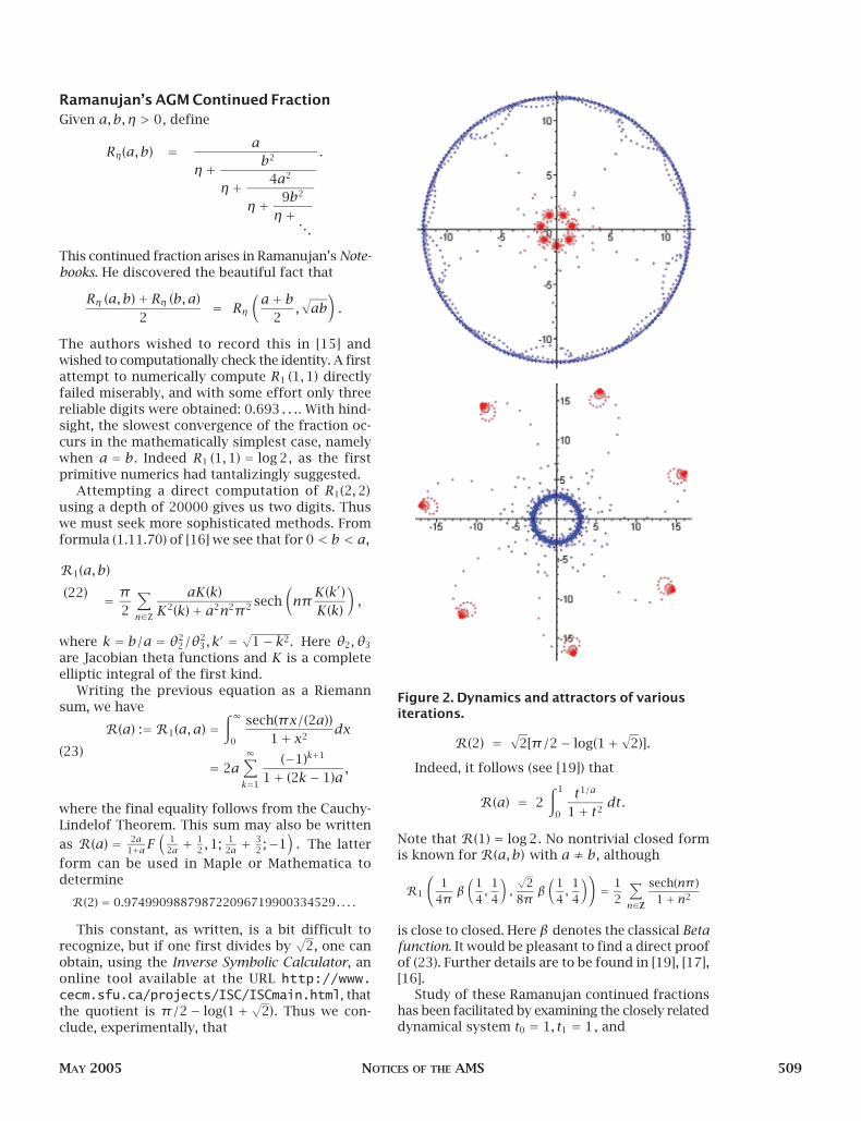
Figure 2. Dynamics and attractors of variousiterations.

510 NOTICES OF THE AMS VOLUME 52, NUMBER 5

tn := tn(a, b) = 1n+ωn−1

(1− 1

n

)tn−2,(24)

where ωn = a2 or b2 (from the Ramanujan con-tinued fraction definition), depending on whethern is even or odd.

If one studies this based only on numerical val-ues, nothing is evident; one only sees that tn → 0fairly slowly. However, if we look at this iterationpictorially, we learn significantly more. In particu-lar, if we plot these iterates in the complex planeand then scale by

√n and color the iterations blue

or red depending on odd or even n, then some re-markable fine structures appear; see Figure 2. Withassistance of such plots, the behavior of these it-erates (and the Ramanujan continued fractions) isnow quite well understood. These studies haveventured into matrix theory, real analysis, and eventhe theory of martingales from probability theory[19], [17], [18], [23].

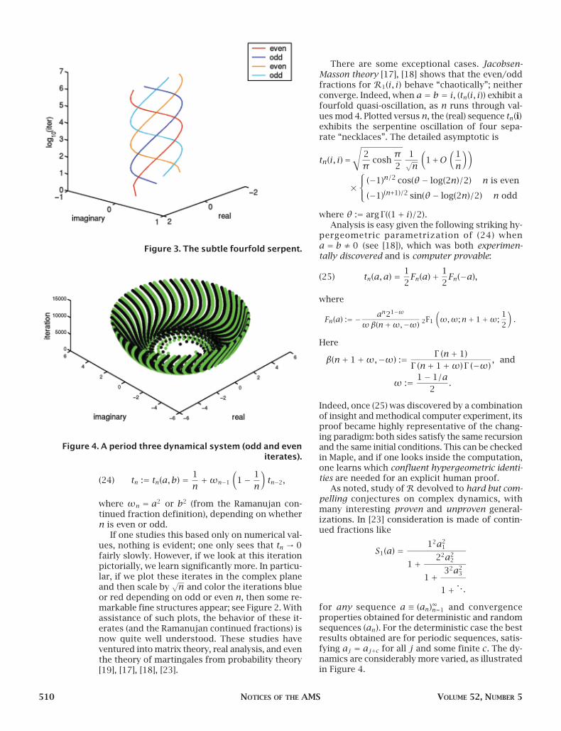
There are some exceptional cases. Jacobsen-Masson theory [17], [18] shows that the even/oddfractions for R1(i, i) behave “chaotically”; neitherconverge. Indeed, when a = b = i, (tn(i, i)) exhibit afourfold quasi-oscillation, as n runs through val-ues mod 4. Plotted versus n, the (real) sequence tn(i)exhibits the serpentine oscillation of four sepa-rate “necklaces”. The detailed asymptotic is

Figure 3. The subtle fourfold serpent.

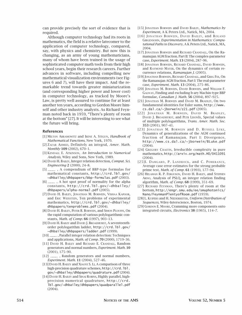
Figure 4. A period three dynamical system (odd and eveniterates).

tn(i, i) =

√2π

coshπ2

1√n

(1 +O

(1n

))

×

(−1)n/2 cos(θ − log(2n)/2) n is even

(−1)(n+1)/2 sin(θ − log(2n)/2) n odd

where θ := arg Γ ((1+ i)/2).Analysis is easy given the following striking hy-

pergeometric parametrization of (24) whena = b ≠ 0 (see [18]), which was both experimen-tally discovered and is computer provable:

tn(a,a) = 12Fn(a)+ 1

2Fn(−a),(25)

where

Fn(a) := − an21−ω

ωβ(n+ω,−ω) 2F1

(ω,ω;n+ 1+ω;

12

).

Here

β(n+ 1+ω,−ω) := Γ (n+ 1)Γ (n+ 1+ω) Γ (−ω)

, and

ω := 1− 1/a2

.

Indeed, once (25) was discovered by a combinationof insight and methodical computer experiment, itsproof became highly representative of the chang-ing paradigm: both sides satisfy the same recursionand the same initial conditions. This can be checkedin Maple, and if one looks inside the computation,one learns which confluent hypergeometric identi-ties are needed for an explicit human proof.

As noted, study of R devolved to hard but com-pelling conjectures on complex dynamics, withmany interesting proven and unproven general-izations. In [23] consideration is made of contin-ued fractions like

S1(a) = 12a21

1+ 22a22

1+ 32a23

1+ . . .

for any sequence a ≡ (an)∞n=1 and convergenceproperties obtained for deterministic and randomsequences (an). For the deterministic case the bestresults obtained are for periodic sequences, satis-fying aj = aj+c for all j and some finite c. The dy-namics are considerably more varied, as illustratedin Figure 4.

MAY 2005 NOTICES OF THE AMS 511

Coincidence and FraudCoincidences do occur, and such examples drivehome the need for reasonable caution in this en-terprise. For example, the approximations

π ≈ 3√163

log(640320), π ≈√

298014412

occur for deep number theoretic reasons: the firstgood to fifteen places, the second to eight. By con-trast

eπ −π = 19.999099979189475768 . . . ,

most probably for no good reason. This seemedmore bizarre on an eight-digit calculator. Likewise,as spotted by Pierre Lanchon recently,

e = 10.10110111111000010101000101100 . . .

while

π = 11.0010010000111111011010101000 . . .

have 19 bits agreeing in base two—with one readingright to left. More extended coincidences are almostalways contrived, as illustrated by the following:

∞∑n=1

[n tanh(π/2)]10n

≈ 181,

∞∑n=1

[n tanh(π )]10n

≈ 181.

The first holds to 12 decimal places, while the sec-ond holds to 268 places. This phenomenon can beunderstood by examining the continued fraction ex-pansion of the constants tanh(π/2) and tanh(π ):the integer 11 appears as the third entry of the first,while 267 appears as the third entry of the second.

Bill Gosper, commenting on the extraordinary ef-fectiveness of continued-fraction expansions to“see” what is happening in such problems, de-clared, “It looks like you are cheating God some-how.”

A fine illustration is the unremarkable decimalα = 1.4331274267223117583 . . . whose contin-ued fraction begins [1,2,3,4,5,6,7,8,9 . . .] and somost probably is a ratio of Bessel functions. Indeed,I0(2)/I1(2) was what generated the decimal. Simi-larly, π and e are quite different as continued frac-tions, less so as decimals.

A more sobering example of high-precision“fraud” is the integral

π2 :=∫∞

0cos(2x)

∞∏n=1

cos(xn

)dx.(26)

The computation of a high-precision numericalvalue for this integral is rather challenging, due inpart to the oscillatory behavior of

∏n≥1 cos(x/n)

(see Figure 2), but mostly due to the difficulty ofcomputing high-precision evaluations of the inte-grand function. Note that evaluating thousands ofterms of the infinite product would produce only

a few correct digits. Thus it is necessary to rewritethe integrand function in a form more suitable forcomputation. This can be done by writing

f (x) = cos(2x)

m∏

1

cos(x/k)

exp(fm(x)),(27)

where we choose m > x , and where

fm(x) =∞∑

k=m+1

log cos(xk

).(28)

The log cos evaluation can be expanded in a Tay-lor series [1, p. 75], as follows:

log cos(xk

)=

∞∑j=1

(−1) j22j−1(22j − 1)B2j

j(2j)!

(xk

)2j,

where B2j are Bernoulli numbers. Note that sincek > m > x in (28), this series converges. We can nowwrite

fm(x) =∞∑

k=m+1

∞∑j=1

(−1) j22j−1(22j − 1)B2j

j(2j)!

(xk

)2j

= −∞∑j=1

(22j − 1)ζ(2j)jπ2j

∞∑k=m+1

1k2j

x2j

= −∞∑j=1

(22j − 1)ζ(2j)jπ2j

ζ(2j)−

m∑k=1

1k2j

x2j .

This can now be written in a compact form for com-putation as

fm(x) = −∞∑j=1

ajbj,mx2j ,(29)

where

(30)

aj =(22j − 1)ζ(2j)

jπ2j ,

bj,m = ζ(2j)−m∑k=1

1/k2j .

n=2n=5n=10

C(x)

–0.2

0

0.2

0.4

0.6

0.8

1

1 2 3 4x

Figure 5. First few terms of ∏n≥1 cos(x/k) .

512 NOTICES OF THE AMS VOLUME 52, NUMBER 5

Computation of these b coefficients must be doneto a much higher precision than that desired forthe quadrature result, since two very nearly equalquantities are subtracted here.

The integral can now be computed using, for ex-ample, the tanh-sinh quadrature scheme. The first60 digits of the result are the following:

0.3926990816987241548078304229099

37860524645434187231595926812 . . . .At first glance, this appears to be π/8. But a care-ful comparison with a high-precision value of π/8,namely

0.3926990816987241548078304229099

37860524646174921888227621868 . . . ,

reveals that they are not equal: the two values dif-fer by approximately 7.407× 10−43. Indeed, thesetwo values are provably distinct. The reason is governed by the fact that

∑55n=1 1/(2n+ 1) > 2 >∑54

n=1 1/(2n+ 1). See [16, Chap. 2] for additionaldetails.

A related example is the following. Recall the sincfunction

sinc(x) := sinxx.

Consider the seven highly oscillatory integralsbelow.

I1 :=∫∞

0sinc(x)dx = π

2,

I2 :=∫∞

0sinc(x)sinc

(x3

)dx = π

2,

I3 :=∫∞

0sinc(x)sinc

(x3

)sinc

(x5

)dx = π

2,

. . .

I6 :=∫∞

0sinc(x)sinc

(x3

)· · · sinc

( x11

)dx = π

2,

I7 :=∫∞

0sinc(x)sinc

(x3

)· · · sinc

( x13

)dx = π

2.

However,

I8 :=∫∞

0sinc(x)sinc

(x3

)· · · sinc

( x15

)dx

= 467807924713440738696537864469935615849440640907310521750000

π

≈ 0.499999999992646π.

When this was first found by a researcher using awell-known computer algebra package, both heand the software vendor concluded there was a“bug” in the software. Not so! It is easy to see thatthe limit of these integrals is 2π1, where

π1 :=∫∞

0cos(x)

∞∏n=1

cos(xn

)dx.(31)

This can be seen via Parseval’s theorem, whichlinks the integral

IN :=∫∞

0sinc(a1x)sinc (a2x) · · · sinc (aNx) dx

with the volume of the polyhedron PN given by

PN := {x : |N∑k=2

akxk| ≤ a1, |xk| ≤ 1,2 ≤ k ≤ N},

where x := (x2, x3, · · · , xN ). If we let

CN := {(x2, x3, · · · , xN ) : −1 ≤ xk ≤ 1,2 ≤ k ≤ N},then

IN = π2a1

Vol(PN )Vol(CN )

.

Thus, the value drops precisely when the con-straint

∑Nk=2 akxk ≤ a1 becomes active and bites

the hypercube CN . That occurs when ∑Nk=2 ak > a1.

In the above, 13 +15 + · · · +

113 < 1, but on addition

of the term 115, the sum exceeds 1, the volume

drops, and IN = π2 no longer holds. A similar analy-

sis applies to π2. Moreover, it is fortunate that webegan with π1 or the falsehood of the identity anal-ogous to that displayed above would have beenmuch harder to see.

Further Directions and ImplicationsIn spite of the examples of the previous section, itmust be acknowledged that computations can inmany cases provide very compelling evidence formathematical assertions. As a single example, re-cently Yasumasa Kanada of Japan calculated π toover one trillion decimal digits (and also to over onetrillion hexadecimal digits). Given that such com-putations—which take many hours on large, state-of-the-art supercomputers—are prone to manytypes of error, including hardware failures, systemsoftware problems, and especially programmingbugs, how can one be confident in such results?

In Kanada’s case, he first used two differentarctangent-based formulas to evaluate π to overone trillion hexadecimal digits. Both calculations

Figure 6. Advanced Collaborative Environment in Vancouver.

MAY 2005 NOTICES OF THE AMS 513

agreed that the hex expansion beginning at position 1,000,000,000,001 is B4466E8D215388C4E014. He then applied a variant of the BBPformula for π , mentioned in Section 3, to calculatethese hex digits directly. The result agreed exactly.Needless to say, it is exceedingly unlikely that three different computations, each using a com-pletely distinct computational approach, would all perfectly agree on these digits unless all threeare correct.

Another, much more common, example is theusage of probabilistic primality testing schemes.Damgard, Landrock, and Pomerance showed in1993 that if an integer n has k bits, then the prob-ability that it is prime, provided it passes the mostcommonly used probabilistic test, is greater than1− k242−

√k , and for certain k is even higher [25].

For instance, if n has 500 bits, then this probabil-ity is greater than 1− 1/428m . Thus a 500-bit integer that passes this test even once is prime with prohibitively safe odds: the chance of a falsedeclaration of primality is less than one part in Avo-gadro’s number (6× 1023) . If it passes the test forfour pseudorandomly chosen integers a, then thechance of false declaration of primality is less thanone part in a googol (10100) . Such probabilities aremany orders of magnitude more remote than thechance that an undetected hardware or softwareerror has occurred in the computation. Such meth-ods thus draw into question the distinction be-tween a probabilistic test and a “provable” test.

Another interesting question is whether theseexperimental methods may be capable of discov-ering facts that are fundamentally beyond the reachof formal proof methods, which, due to Gödel’s re-sult, we know must exist; see also [24].

One interesting example, which has arisen in ourwork, is the following. We mentioned in Section 3the fact that the question of the 2-normality of πreduces to the question of whether the chaotic it-eration x0 = 0 and

xn ={

16xn−1 +120n2 − 89n+ 16

512n4 − 1024n3 + 712n2 − 206n+ 21

},

where {·} denotes fractional part, are equidistrib-uted in the unit interval.

It turns out that if one defines the sequenceyn = �16xn� (in other words, one records which ofthe 16 subintervals of (0,1), numbered 0 through15, xn lies in), that the sequence (yn), when inter-preted as a hexadecimal string, appears to pre-cisely generate the hexadecimal digit expansion ofπ . We have checked this to 1,000,000 hex digits andhave found no discrepancies. It is known that (yn)is a very good approximation to the hex digits ofπ , in the sense that the expected value of the num-ber of errors is finite [15, Section 4.3] [11]. Thusone can argue, by the second Borel-Cantelli lemma,that in a heuristic sense the probability that there

is any error among the remaining digits after thefirst million is less than 1.465× 10−8 [15, Section4.3]. Additional computations could be used tolower this probability even more.

Although few would bet against such odds, thesecomputations do not constitute a rigorous proofthat the sequence (yn) is identical to the hexadec-imal expansion of π . Perhaps someday someonewill be able to prove this observation rigorously.On the other hand, maybe not—maybe this observation is in some sense an “accident” of mathematics, for which no proof will ever be found. Perhaps numerical validation is all we canever achieve here.

ConclusionWe are only now beginning to digest some very oldideas:

Leibniz’s idea is very simple and veryprofound. It’s in section VI of the Dis-cours [de métaphysique]. It’s the obser-vation that the concept of law becomesvacuous if arbitrarily high mathemati-cal complexity is permitted, for thenthere is always a law. Conversely, if thelaw has to be extremely complicated,then the data is irregular, lawless, ran-dom, unstructured, patternless, andalso incompressible and irreducible. Atheory has to be simpler than the datathat it explains, otherwise it doesn’t ex-plain anything. —Gregory Chaitin [24]

Chaitin argues convincingly that there are manymathematical truths which are logically and com-putationally irreducible—they have no good reasonin the traditional rationalist sense. This in turnadds force to the desire for evidence even whenproof may not be possible. Computer experiments

Figure 7. Polyhedra in an immersive environment.

514 NOTICES OF THE AMS VOLUME 52, NUMBER 5

can provide precisely the sort of evidence that isrequired.

Although computer technology had its roots inmathematics, the field is a relative latecomer to theapplication of computer technology, compared,say, with physics and chemistry. But now this ischanging, as an army of young mathematicians,many of whom have been trained in the usage ofsophisticated computer math tools from their highschool years, begin their research careers. Furtheradvances in software, including compelling newmathematical visualization environments (see Fig-ures 6 and 7), will have their impact. And the re-markable trend towards greater miniaturization(and corresponding higher power and lower cost)in computer technology, as tracked by Moore’sLaw, is pretty well assured to continue for at leastanother ten years, according to Gordon Moore him-self and other industry analysts. As Richard Feyn-man noted back in 1959, “There’s plenty of roomat the bottom” [27]. It will be interesting to see whatthe future will bring.

References[1] MILTON ABRAMOWITZ and IRENE A. STEGUN, Handbook of

Mathematical Functions, New York, 1970.[2] ZAFAR AHMED, Definitely an integral, Amer. Math.

Monthly 109 (2002), 670–1.[3] KENDALL E. ATKINSON, An Introduction to Numerical

Analysis, Wiley and Sons, New York, 1989.[4] DAVID H. BAILEY, Integer relation detection, Comput. Sci.

Engineering 2 (2000), 24–8.[5] ——— , A compendium of BBP-type formulas for

mathematical constants, http://crd.lbl.gov/~dhbailey/dhbpapers/bbp-formulas.pdf (2003).

[6] ——— , A hot spot proof of normality for the alpha constants, http://crd.lbl.gov/~dhbailey/dhbpapers/alpha-normal.pdf (2005).

[7] DAVID H. BAILEY, JONATHAN M. BORWEIN, VISHAA KAPOOR, and ERIC WEISSTEIN, Ten problems of experimental mathematics, http://crd.lbl.gov/~dhbailey/dhbpapers/tenproblems.pdf (2004).

[8] DAVID H. BAILEY, PETER B. BORWEIN, and SIMON PLOUFFE, Onthe rapid computation of various polylogarithmic con-stants, Math. of Comp. 66 (1997), 903–13.

[9] DAVID H. BAILEY and DAVID J. BROADHURST, A seventeenth-order polylogarithm ladder, http://crd.lbl.gov/~dhbailey/dhbpapers/ladder.pdf (1999).

[10] ——— , Parallel integer relation detection: Techniquesand applications, Math. of Comp. 70 (2000), 1719–36.

[11] DAVID H. BAILEY and RICHARD E. CRANDALL, Randomgenerators and normal numbers, Experiment. Math. 10(2001), 175–90.

[12] ——— , Random generators and normal numbers, Experiment. Math. 11 (2004), 527–46.

[13] DAVID H. BAILEY and XIAOYE S. LI, A comparison of threehigh-precision quadrature schemes, http://crd.lbl.gov/~dhbailey/dhbpapers/quadrature.pdf (2004).

[14] DAVID H. BAILEY and SINAI ROBINS, Highly parallel, high-precision numerical quadrature, http://crd.lbl.gov/~dhbailey/dhbpapers/quadparallel.pdf(2004).

[15] JONATHAN BORWEIN and DAVID BAILEY, Mathematics byExperiment, A K Peters Ltd., Natick, MA, 2004.

[16] JONATHAN BORWEIN, DAVID BAILEY, and ROLAND

GIRGENSOHN, Experimentation in Mathematics: Compu-tational Paths to Discovery, A K Peters Ltd., Natick, MA,2004.

[17] JONATHAN BORWEIN and RICHARD CRANDALL, On the Ra-manujan AGM fraction. Part II: The complex-parametercase, Experiment. Math. 13 (2004), 287–96.

[18] JONATHAN BORWEIN, RICHARD CRANDALL, DAVID BORWEIN,and RAYMOND MAYER, On the dynamics of certain re-currence relations, Ramanujan J. (2005).

[19] JONATHAN BORWEIN, RICHARD CRANDALL, and GREG FEE, Onthe Ramanujan AGM fraction. Part I: The real-parametercase, Experiment. Math. 13 (2004), 275–86.

[20] JONATHAN M. BORWEIN, DAVID BORWEIN, and WILLIAM F. GALWAY, Finding and excluding b-ary Machin-type BBPformulae, Canadian J. Math. 56 (2004), 897–925.

[21] JONATHAN M. BORWEIN and DAVID M. BRADLEY, On twofundamental identities for Euler sums, http://www.cs.dal.ca/~jborwein/z21.pdf (2005).

[22] JONATHAN M. BORWEIN, DAVID M. BRADLEY, DAVID J. BROADHURST, and PETR LISONEK, Special valuesof multiple polylogarithms, Trans. Amer. Math. Soc.353 (2001), 907–41.

[23] JONATHAN M. BORWEIN and D. RUSSELL LUKE, Dynamics of generalizations of the AGM continuedfraction of Ramanujan. Part I: Divergence,http://www.cs.dal.ca/~jborwein/BLuke.pdf(2004).

[24] GREGORY CHAITIN, Irreducible complexity in pure mathematics, http://arxiv.org/math.HO/0411091(2004).

[25]I. DAMGARD, P. LANDROCK, and C. POMERANCE, Average case error estimates for the strong probableprime test, Math. of Comp. 61 (1993), 177–94.

[26] HELAMAN R. P. FERGUSON, DAVID H. BAILEY, and STEPHEN

ARNO, Analysis of PSLQ, an integer relation finding algorithm, Math. of Comp. 68 (1999), 351–69.

[27] RICHARD FEYNMAN, There’s plenty of room at the bottom, http://engr.smu.edu/ee/smuphotonics/Nano/FeynmanPlentyofRoom.pdf (1959).

[28] L. KUIPERS and H. NIEDERREITER, Uniform Distribution ofSequences, Wiley-Interscience, Boston, 1974.

[29] GORDON E. MOORE, Cramming more components ontointegrated circuits, Electronics 38 (1965), 114–7.