experimental measurement of dielectric properties of
TRANSCRIPT

Graduate Theses, Dissertations, and Problem Reports
2019
Experimental Measurement of Dielectric Properties of Powdery Experimental Measurement of Dielectric Properties of Powdery
Materials using a Coaxial Transmission Line Materials using a Coaxial Transmission Line
Robert Tempke [email protected]
Follow this and additional works at: https://researchrepository.wvu.edu/etd
Part of the Mechanical Engineering Commons, and the Other Materials Science and Engineering
Commons
Recommended Citation Recommended Citation Tempke, Robert, "Experimental Measurement of Dielectric Properties of Powdery Materials using a Coaxial Transmission Line" (2019). Graduate Theses, Dissertations, and Problem Reports. 3933. https://researchrepository.wvu.edu/etd/3933
This Thesis is protected by copyright and/or related rights. It has been brought to you by the The Research Repository @ WVU with permission from the rights-holder(s). You are free to use this Thesis in any way that is permitted by the copyright and related rights legislation that applies to your use. For other uses you must obtain permission from the rights-holder(s) directly, unless additional rights are indicated by a Creative Commons license in the record and/ or on the work itself. This Thesis has been accepted for inclusion in WVU Graduate Theses, Dissertations, and Problem Reports collection by an authorized administrator of The Research Repository @ WVU. For more information, please contact [email protected].
Experimental Measurement of Dielectric Properties of Powdery Materials using a Coaxial
Transmission Line
Robert Sean Tempke
Thesis submitted
to the Benjamin M. Statler College of
Engineering and Mineral Resources
at West Virginia University
in partial fulfillment of the requirements for the degree of
Master of Science
in
Mechanical Engineering
Terence Musho, Ph.D., Chair
Edward Sabolsky, Ph.D.
Christina Wildfire, Ph.D.
Department of Mechanical and Aerospace Engineering
Morgantown, West Virginia
May 2019
Keywords: Composite, Dielectric Constant, Microwave, Paraffin, Standardized Method,
Dielectric Properties
Copyright 2019 Robert Sean Tempke
ABSTRACT
Experimental Measurement of Dielectric Properties of Powdery Materials using a Coaxial
Transmission Line
Robert Tempke
This study proposes a standard methodology for coaxial dielectric property measurements of
powdery materials (1-10GHz) using a coaxial transmission line. Four powdery materials with
dielectric constants ranging from 3.5 to 70 (SiO2, Al2O3, CeO2, and TiO2) were experimentally
investigated at varying volume loading fractions in a paraffin mixture. A statistically significant
number of paraffin heterogeneous-mixtures was synthesized for all dielectric powders. The
dielectric properties of the constitutive materials were determined using appropriate mixture
equations. The sensitivity of the equations dielectric prediction to volume loading is discussed
with guidance on selecting the best mixing equation. It was determined that low volume loadings
of less than 10% was ideal for a general case where little to nothing is known about the sample. If
the general range of the dielectric constant is known different mixture equations were found to be
optimal for specific ranges. Furthermore, there was not a single mixing equation that proved best
over the entire range of dielectrics studied. To this end, a standard testing procedure for powdery
materials is justified, with guidelines for selection of an appropriate mixture equation. The
justification is based on the ratio of the dielectric constant of the powder to that of the paraffin.
These findings provide a baseline procedure for determining dielectric properties of new powdery
materials that have applications in the area of microwave catalysis.

iii
To my family the ones I was born with and the ones I chose.
Thank you to Rhiannon Schmitt for all the support and love you have shown me while I worked
late into the night.
iv
ACKNOWLEDGMENTS
First and foremost, I would like to thank my advisor and mentor Dr. Terence D. Musho for
all his support and guidance in leading me through my research. His guidance and advice were
paramount to my success and growth over these last few years. I look forward to continuing out
work together as we move forward on new and exciting projects.
I would also like to give special thanks to Dr. Christina Wildfire who mentored me and
showed me the importance of experimental lab work. I made frequent use of her open door to ask
her a constant barrage of questions which she tirelessly answered. If not for her I would still be in
the lab trying to figure out what was going on.
A special thanks is required for all my colleagues at NETL, who despite some less than
conventional motivational methods were of great help in all my research. One thing I would like
to remember is donuts are not free.
v
Table of Contents
LIST OF FIGURES ................................................................................................................................... ix
LIST OF TABLES ................................................................................................................................... xiii
CHAPTER 1: INTRODUCTION .............................................................................................................. 1
1.1 Background ..................................................................................................................................... 1
1.2 Objective .......................................................................................................................................... 2
1.3 Significance ...................................................................................................................................... 3
CHAPTER 2: TECHNOLOGY AND THEORY ..................................................................................... 4
2.1 Microwave Technology ............................................................................................................... 4
2.1.1 Microwaves .......................................................................................................................... 4
2.2 Microwave Material Interactions .............................................................................................. 5
2.2.1 Permittivity .......................................................................................................................... 7
2.2.2 Permeability ......................................................................................................................... 8
2.2.3 Microscopic, Local and Macroscopic Fields ..................................................................... 9
2.2.4 Local Electromagnetic Fields in Materials ....................................................................... 9
2.3 Measurement Models for Material Properties ....................................................................... 10
2.3.1 Transmission/Reflection measurement techniques for lossy materials ........................ 10
2.3.2 Scattering Parameters ...................................................................................................... 10
2.4 Instrumentation ......................................................................................................................... 11
2.4.1 Coaxial Line ....................................................................................................................... 11
2.4.2 Waveguide ......................................................................................................................... 12
2.4.3 Free Space .......................................................................................................................... 13
2.4.4 Coaxial Probe Method ...................................................................................................... 14
2.4.5 Network Analyzers ............................................................................................................ 15
2.5 Error........................................................................................................................................... 16
2.5.1 Random Uncertainties and Error .................................................................................... 16
2.5.2 Systematic Uncertainties .................................................................................................. 16
2.5.3 Corrections to Data ........................................................................................................... 16
2.6 Permeability and Permittivity Calculations ........................................................................... 17
2.6.1 Nicolson-Ross-Weir ........................................................................................................... 17
2.6.2 Nicolson-Ross-Weir Polynomial Method ........................................................................ 17
2.6.3 NIST Iterative Solution .................................................................................................... 17
2.6.4 NIST Non-Iterative ........................................................................................................... 17
2.6.5 Short Circuit Line ............................................................................................................. 18
vi
2.7 Microwave Heating ................................................................................................................... 18
2.8 Powdery Materials .................................................................................................................... 18
2.9 Specimen Preparations for Powdery Material ....................................................................... 19
2.9.1 Sintering ............................................................................................................................. 19
2.9.2 Pressing .............................................................................................................................. 19
2.9.3 Paraffin Matrix ................................................................................................................. 20
2.10 Mixture equations for Two Phase Homogenous Composites ................................................ 21
2.10.1 Parallel Mixing Equation ................................................................................................. 21
2.10.2 Series Mixing Equation .................................................................................................... 21
2.10.3 Logarithmic Mixing Equation ......................................................................................... 22
2.10.4 Lichtenecker Mixing Equation ........................................................................................ 22
2.10.5 Looyenga Mixing Equation .............................................................................................. 22
2.10.6 Birchak Mixing Equation ................................................................................................. 22
2.10.7 Poon-Shin Mixing Equation ............................................................................................. 22
2.10.8 Effective Medium Theory Mixing Equation ................................................................... 23
2.10.9 Maxwell-Garnet Mixing Equation .................................................................................. 23
2.10.10 Jayasundere-Smith Mixing Equation .......................................................................... 23
2.11 Dielectric Constant Bounds ...................................................................................................... 24
2.11.1 Wiener Bounds .................................................................................................................. 24
2.11.2 Hashin-Shtrikman Bounds ............................................................................................... 24
CHAPTER 3: EXPERIMENTAL TESING OF POWDERY MATERIALS ..................................... 26
3.1 Powder Selection ....................................................................................................................... 26
3.2 Sample Preparation .................................................................................................................. 26
3.2.1 Casting Mold Creation ..................................................................................................... 26
3.2.2 Volume Loading Selection ................................................................................................ 27
3.2.3 Composite Mixing ............................................................................................................. 27
3.2.4 Curing Process................................................................................................................... 28
3.3 Testing Parameters ................................................................................................................... 28
3.4 Sample Testing .......................................................................................................................... 28
3.4.1 Testing Cell Preparation .................................................................................................. 28
3.4.2 Sample Loading in Coaxial Test Cell .............................................................................. 28
3.4.3 Testing Initiation ............................................................................................................... 29
3.5 CT Imaging ................................................................................................................................ 30
3.5.1 Dispersion Verification ..................................................................................................... 30
3.5.2 Volume Loading Verification ........................................................................................... 31

vii
CHAPTER 4: EXPERIMENTAL DIELECTRIC TESTING RESULTS ........................................... 33
4.1 Silicon Dioxide Composite Testing Results ............................................................................. 33
4.1.1 Theoretical Parallel Mixing Equation Results for SiO2 ................................................. 33
4.1.2 Theoretical Series Mixing Equation Results for SiO2 .................................................... 35
4.1.3 Theoretical Logarithmic Mixing Equation Results for SiO2 ......................................... 36
4.1.4 Theoretical Lichtenecker Mixing Equation for SiO2 ..................................................... 37
4.1.5 Theoretical Looyenga Mixing Equation for SiO2 ........................................................... 38
4.1.6 Theoretical Birchak Mixing Equation for SiO2 .............................................................. 39
4.1.7 Theoretical Poon-Shin Mixing Equation for SiO2 .......................................................... 40
4.1.8 Theoretical Effective Medium Theory Mixing Equation for SiO2................................ 41
4.1.9 Theoretical Maxwell-Garnett Mixing Equation for SiO2 .............................................. 42
4.1.10 Theoretical Jayasundere-Smith Mixing Equation for SiO2 .......................................... 43
4.2 Aluminum Oxide Dioxide Composite Testing Results ........................................................... 44
4.2.1 Theoretical Parallel Mixing Equation Results for Al2O3 ............................................... 44
4.2.2 Theoretical Series Mixing Equation Results for Al2O3 .................................................. 46
4.2.3 Theoretical Logarithmic Mixing Equation Results for Al2O3 ....................................... 47
4.2.4 Theoretical Lichtenecker Mixing Equation for Al2O3 ................................................... 48
4.2.5 Theoretical Looyenga Mixing Equation for Al2O3 ......................................................... 49
4.2.6 Theoretical Birchak Mixing Equation for Al2O3 ............................................................ 50
4.2.7 Theoretical Poon-Shin Mixing Equation for Al2O3 ........................................................ 51
4.2.8 Theoretical Effective Medium Theory Mixing Equation for Al2O3 .............................. 52
4.2.9 Theoretical Maxwell-Garnet Mixing Equation for Al2O3 ............................................. 53
4.2.10 Theoretical Jayasundere-Smith Mixing Equation for Al2O3 ........................................ 54
4.3 Cerium Dioxide Composite Testing Results ........................................................................... 55
4.3.1 Theoretical Parallel Mixing Equation Results for CeO2 ............................................... 55
4.3.2 Theoretical Series Mixing Equation Results for CeO2 .................................................. 57
4.3.3 Theoretical Logarithmic Mixing Equation Results for CeO2 ....................................... 58
4.3.4 Theoretical Lichtenecker Mixing Equation for CeO2 .................................................... 59
4.3.5 Theoretical Looyenga Mixing Equation for CeO2 ......................................................... 60
4.3.6 Theoretical Birchak Mixing Equation for CeO2 ............................................................ 61
4.3.7 Theoretical Poon-Shin Mixing Equation for CeO2 ........................................................ 62
4.3.8 Theoretical Effective Medium Theory Mixing Equation for CeO2 .............................. 63
4.3.9 Theoretical Maxwell-Garnet Mixing Equation for CeO2 .............................................. 64
4.3.10 Theoretical Jayasundere-Smith Mixing Equation for CeO2 ......................................... 65
4.4 Titanium Dioxide Composite Testing Results ........................................................................ 66
viii
4.4.1 Theoretical Parallel Mixing Equation Results for TiO2 ................................................ 66
4.4.2 Theoretical Series Mixing Equation Results for TiO2 ................................................... 68
4.4.3 Theoretical Logarithmic Mixing Equation Results for TiO2 ........................................ 69
4.4.4 Theoretical Lichtenecker Mixing Equation for TiO2 ..................................................... 70
4.4.5 Theoretical Looyenga Mixing Equation for TiO2 .......................................................... 71
4.4.6 Theoretical Birchak Mixing Equation for TiO2 ............................................................. 72
4.4.7 Theoretical Poon-Shin Mixing Equation for TiO2 ......................................................... 73
4.4.8 Theoretical Effective Medium Theory Mixing Equation for TiO2 ............................... 74
4.4.9 Theoretical Maxwell-Garnett Mixing Equation for TiO2.............................................. 75
4.4.10 Theoretical Jayasundere-Smith Mixing Equation for TiO2 .......................................... 76
CHAPTER 5: CONCLUSION ................................................................................................................. 77
5.1 Summary of Research ............................................................................................................... 77
5.2 Future Directions ...................................................................................................................... 79
References .................................................................................................................................................. 80
ix
LIST OF FIGURES
Figure 2.1: Electromagnetic spectrum with a visualization of the visible spectrum
shown as a subset of electromagnetic radiation ......................................................................... 4
Figure 2.2: An electromagnetic wave propagating in the +z direction through a homogenous,
isotropic, dissipationless medium. The wave is linearly polarized, where the electric field is
shown in blue and the magnetic field is shown in red. The electric field oscillates in the ±x
direction while the magnetic field oscillates in the ±y direction ............................................... 5
Figure 2.3: a: electrical conducting material, b: insulating material, c: dielectric material16. . .7
Figure 2.4: Dielectric permittivity spectrum over a wide range of frequencies. Various processes
are labeled on the image: ionic and dipolar relaxation, atomic and electronic resonances at higher
energies67.................................................................................................................................... 8
Figure 2.5 Single wave in a two-port electrical-element. Simple representation of a standard 2
port measurement for S-parameters31 ........................................................................................ 11
Figure 2.6: Keysight Network high precision coaxial airline. Used to measure the scattering
parameters and calculate the associated material properties. Example of a testable material is
shown as the composite34 ........................................................................................................... 12
Figure 2.7: Waveguides for use in vector network analyzer, shown are both a circular and
rectangular waveguide68............................................................................................................. 13
Figure 2.8: Illustration of the Free space method during testing of material properties30 ........ 14
Figure 2.9: Standard Keysight High Temperature Coaxial Probe, used to collect scattering
parameters from a material so a VNA can calculate the material properties28 .......................... 15
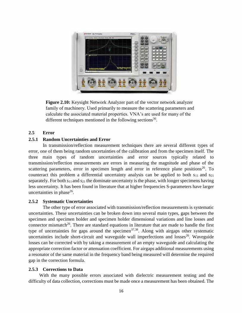
Figure 2.10: Keysight Network Analyzer part of the vector network analyzer family of
machinery. Used primarily to measure the scattering parameters and calculate the associated
material properties. VNA’s are used for many of the different techniques mentioned in the
following sections34 ................................................................................................................... 16
Figure 2.11: (a) Alumina pellet with individual grains, (b) well sintered pellet with defined
cleavage plans at 1580 ºC48 ........................................................................................................ 19
Figure 2.12: Effects of particle size on both hot isostatic pressing and cold isostatic
pressing51.................................................................................................................................... 20
Figure 2.13: The maximum effective permittivity for a given volume fraction of inclusions
manifest if the inclusions are in the direction of the flux as shown on the left side. The minimum
effective permittivity for a given volume fraction of inclusions corresponds to when the flux is
forced to pass through the phase with lower permittivity56 ....................................................... 24
Figure 2.14: Wiener bounds and Hashin-Shtrikman bounds for dielectric constant of a mixture
with a dielectric inclusion of 1024 .............................................................................................. 25
x
Figure 3.1: (A) 3-D rendering of casting mold for paraffin composite mixtures. The molds are
reusable and provide consistency from batch to batch production. (B) The final 3D printed
product with a composite mold attached for visualization ........................................................ 27
Figure 3.2: Paraffin-powder material composite plug loaded into the precision airline. The plug
fills all the space between the center electrode and the outer electrode to ensure no airgaps
exist ............................................................................................................................................ 29
Figure 3.3: VNA setup for high precision coaxial airline testing. Two port VNA with a 10 CM
testing line .................................................................................................................................. 30
Figure 3.4: Cross sectional view of an Al2O3 that allows for a visual confirmation of powder
distribution within the paraffin matrix. The lines on the bottom are a consequence of beam
hardening in the CT scanner66 .................................................................................................... 31
Figure 3.5: 3D rendering from CT images of a CeO2 30% volume loading composite.
Reconstruction was preformed using FIJI and volume loading was verified using there built in
software66 ................................................................................................................................... 32
Figure 4.1: Theoretical Parallel Mixture equation for SiO2 mapped against experimental scatter
plot data for four different volume loadings .............................................................................. 34
Figure 4.2: Theoretical Series Mixture equation for SiO2 mapped against experimental scatter
plot data for four different volume loadings .............................................................................. 35
Figure 4.3: Theoretical Logarithmic Mixture equation for SiO2 mapped against experimental
scatter plot data for four different volume loadings ................................................................... 36
Figure 4.4: Theoretical Lichtenecker mixture equation for SiO2 mapped against experimental
scatter plot data for four different volume loadings ................................................................... 37
Figure 4.5: Theoretical Looyenga mixture equation for SiO2 mapped against experimental
scatter plot data for four different volume loadings ................................................................... 38
Figure 4.6: Theoretical Birchak mixture equation for SiO2 mapped against experimental scatter
plot data for four different volume loadings .............................................................................. 39
Figure 4.7: Theoretical Poon-Shin Mixture equation for SiO2 mapped against experimental
scatter plot data for four different volume loadings ................................................................... 40
Figure 4.8: Theoretical EMT mixture equation for SiO2 mapped against experimental scatter
plot data for four different volume loadings .............................................................................. 41
Figure 4.9: Theoretical Maxwell-Garnett mixture equation for SiO2 mapped against
experimental scatter plot data for four different volume loadings ............................................. 42
Figure 4.10: Theoretical Jayasundere-Smith mixture equation for SiO2 mapped against
experimental scatter plot data for four different volume loadings ............................................. 43
xi
Figure 4.11: Theoretical Parallel Mixture equation for Al2O3 mapped against experimental
scatter plot data for four different volume loadings ................................................................... 45
Figure 4.12: Theoretical Series Mixture equation for Al2O3 mapped against experimental
scatter plot data for four different volume loadings ................................................................... 46
Figure 4.13: Theoretical Logarithmic Mixture equation for Al2O3 mapped against experimental
scatter plot data for four different volume loadings ................................................................... 47
Figure 4.14: Theoretical Lichtenecker mixture equation for Al2O3 mapped against experimental
scatter plot data for four different volume loadings ................................................................... 48
Figure 4.15: Theoretical Looyenga mixture equation for Al2O3 mapped against experimental
scatter plot data for four different volume loadings ................................................................... 49
Figure 4.16: Theoretical Birchak mixture equation for Al2O3 mapped against experimental
scatter plot data for four different volume loadings ................................................................... 50
Figure 4.17: Theoretical Poon-Shin Mixture equation for Al2O3 mapped against experimental
scatter plot data for four different volume loadings ................................................................... 51
Figure 4.18: Theoretical EMT mixture equation for Al2O3mapped against experimental scatter
plot data for four different volume loadings .............................................................................. 52
Figure 4.19: Theoretical Maxwell-Garnett mixture equation for Al2O3mapped against
experimental scatter plot data for four different volume loadings ............................................. 53
Figure 4.20: Theoretical Jayasundere-Smith mixture equation for Al2O3mapped against
experimental scatter plot data for four different volume loadings ............................................. 54
Figure 4.21: Theoretical Parallel Mixture equation for CeO2 mapped against experimental
scatter plot data for four different volume loadings ................................................................... 56
Figure 4.22: Theoretical Series Mixture equation for CeO2 mapped against experimental scatter
plot data for four different volume loadings .............................................................................. 57
Figure 4.23: Theoretical Logarithmic Mixture equation for CeO2 mapped against experimental
scatter plot data for four different volume loadings ................................................................... 58
Figure 4.24: Theoretical Lichtenecker mixture equation for CeO2 mapped against experimental
scatter plot data for four different volume loadings ................................................................... 59
Figure 4.25: Theoretical Looyenga mixture equation for CeO2 mapped against experimental
scatter plot data for four different volume loadings ................................................................... 60
Figure 4.26: Theoretical Birchak mixture equation for CeO2 mapped against experimental
scatter plot data for four different volume loadings ................................................................... 61
Figure 4.27: Theoretical Poon-Shin Mixture equation for CeO2 mapped against experimental
scatter plot data for four different volume loadings ................................................................... 62
xii
Figure 4.28: Theoretical EMT mixture equation for CeO2 mapped against experimental scatter
plot data for four different volume loadings .............................................................................. 63
Figure 4.29: Theoretical Maxwell-Garnett mixture equation for CeO2 mapped against
experimental scatter plot data for four different volume loadings ............................................. 64
Figure 4.30: Theoretical Jayasundere-Smith mixture equation for CeO2 mapped against
experimental scatter plot data for four different volume loadings ............................................. 65
Figure 4.31: Theoretical Parallel Mixture equation for CeO2 mapped against experimental
scatter plot data for four different volume loadings ................................................................... 67
Figure 4.32: Theoretical Series Mixture equation for CeO2 mapped against experimental scatter
plot data for four different volume loadings .............................................................................. 68
Figure 4.33: Theoretical Logarithmic Mixture equation for CeO2 mapped against experimental
scatter plot data for four different volume loadings ................................................................... 69
Figure 4.34: Theoretical Lichtenecker mixture equation for CeO2 mapped against experimental
scatter plot data for four different volume loadings ................................................................... 70
Figure 4.35: Theoretical Looyenga mixture equation for CeO2 mapped against experimental
scatter plot data for four different volume loadings ................................................................... 71
Figure 4.36: Theoretical Birchak mixture equation for CeO2 mapped against experimental
scatter plot data for four different volume loadings ................................................................... 72
Figure 4.37: Theoretical Poon-Shin Mixture equation for CeO2 mapped against experimental
scatter plot data for four different volume loadings ................................................................... 73
Figure 4.38: Theoretical EMT mixture equation for CeO2 mapped against experimental scatter
plot data for four different volume loadings .............................................................................. 74
Figure 4.39: Theoretical Maxwell-Garnett mixture equation for CeO2 mapped against
experimental scatter plot data for four different volume loadings ............................................. 75
Figure 4.40: Theoretical Jayasundere-Smith mixture equation for CeO2 mapped against
experimental scatter plot data for four different volume loadings ............................................. 76
xiii
LIST OF TABLES
Table 3.1: Powders used in the study to determine the accuracy of the mixture equations for two-
phase homogenous composites. Associated relevant information such as the supplier, density and
dielectric constant ......................................................................................................................... 26
Table 4.1: Absolute Percent Error for SiO2 composites using Parallel mixing equation ............ 34
Table 4.2: Absolute Percent Error for SiO2 composites using Series mixing equation ............... 35
Table 4.3: Absolute Percent Error for SiO2 composites using Logarithmic mixing equation ..... 36
Table 4.4: Absolute Percent Error for SiO2 composites using Lichtenecker mixing equation .... 37
Table 4.5: Absolute Percent Error for SiO2 composites using Looyenga mixing equation......... 38
Table 4.6: Absolute Percent Error for SiO2 composites using Birchak mixing equation ............ 39
Table 4.7: Absolute Percent Error for SiO2 composites using Poon-Shin mixing equation ........ 40
Table 4.8: Absolute Percent Error for SiO2 composites using EMT mixing equation ................ 41
Table 4.9: Absolute Percent Error for SiO2 composites using Maxwell-Garnett mixing equation
....................................................................................................................................................... 42
Table 4.10: Absolute Percent Error for SiO2 composites using Jayasundere-Smith mixing equation
....................................................................................................................................................... 43
Table 4.11: Absolute Percent Error for Al2O3 composites using Parallel mixing equation ........ 44
Table 4.12: Absolute Percent Error for Al2O3 composites using Series mixing equation ........... 46
Table 4.13: Absolute Percent Error for Al2O3 composites using Logarithmic mixing equation
....................................................................................................................................................... 47
Table 4.14: Absolute Percent Error for Al2O3 composites using Lichtenecker mixing equation
....................................................................................................................................................... 48
Table 4.15: Absolute Percent Error for Al2O3 composites using Looyenga mixing equation ..... 49
Table 4.16: Absolute Percent Error for Al2O3 composites using Birchak mixing equation ........ 50
Table 4.17: Absolute Percent Error for Al2O3 composites using Poon-Shin mixing equation .... 51
Table 4.18: Absolute Percent Error for Al2O3 composites using EMT mixing equation ............ 52
Table 4.19: Absolute Percent Error for Al2O3 composites using Maxwell-Garnett mixing equation
....................................................................................................................................................... 53
Table 4.20: Absolute Percent Error for Al2O3 composites using Jayasundere-Smith mixing
equation ......................................................................................................................................... 54

xiv
Table 4.21: Absolute Percent Error for CeO2 composites using Parallel mixing equation ......... 56
Table 4.22: Absolute Percent Error for CeO2 composites using Series mixing equation ............ 57
Table 4.23: Absolute Percent Error for CeO2 composites using Logarithmic mixing equation .. 58
Table 4.24: Absolute Percent Error for CeO2 composites using Lichtenecker mixing equation
....................................................................................................................................................... 59
Table 4.25: Absolute Percent Error for CeO2 composites using Looyenga mixing equation ..... 60
Table 4.26: Absolute Percent Error for CeO2 composites using Birchak mixing equation ......... 61
Table 4.27: Absolute Percent Error for CeO2 composites using Poon-Shin mixing equation..... 62
Table 4.28: Absolute Percent Error for CeO2 composites using EMT mixing equation ............. 63
Table 4.29: Absolute Percent Error for CeO2 composites using Maxwell-Garnett mixing equation
....................................................................................................................................................... 64
Table 4.30: Absolute Percent Error for CeO2 composites using Jayasundere-Smith mixing
equation ......................................................................................................................................... 65
Table 4.31: Absolute Percent Error for TiO2 composites using Parallel mixing equation .......... 67
Table 4.32: Absolute Percent Error for TiO2 composites using Series mixing equation ............. 68
Table 4.33: Absolute Percent Error for TiO2 composites using Logarithmic mixing equation ... 69
Table 4.34: Absolute Percent Error for TiO2 composites using Lichtenecker mixing equation . 70
Table 4.35: Absolute Percent Error for TiO2 composites using Looyenga mixing equation ...... 71
Table 4.36: Absolute Percent Error for TiO2 composites using Birchak mixing equation .......... 72
Table 4.37: Absolute Percent Error for TiO2 composites using Poon-Shin mixing equation ..... 73
Table 4.38: Absolute Percent Error for TiO2 composites using EMT mixing equation .............. 74
Table 4.39: Absolute Percent Error for TiO2 composites using Maxwell-Garnett mixing equation
....................................................................................................................................................... 75
Table 4.40: Absolute Percent Error for TiO2 composites using Jayasundere-Smith mixing equation
....................................................................................................................................................... 76
Table 5.1: The best mixing equation for each powdery material studied and the associated
averaged error over the volume fractions studied between the equation and the experimental
values. The EMT mixing equation is recommended over the Maxwell-Garnett for simplicity
despite a statistically insignificant improvement of error when using the latter equation............ 78
Table 5.2: Suggested mixing equation based on the ratio of powder’s dielectric properties to
matrix material’s dielectric properties .......................................................................................... 78
1
CHAPTER 1: INTRODUCTION
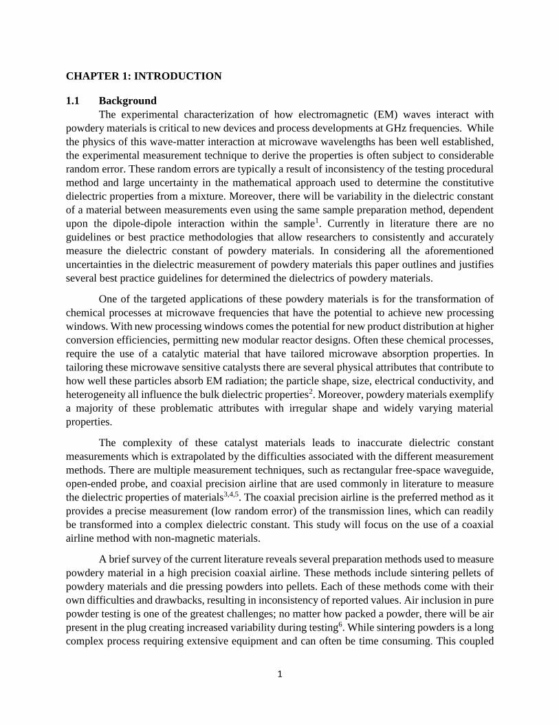
1.1 Background
The experimental characterization of how electromagnetic (EM) waves interact with
powdery materials is critical to new devices and process developments at GHz frequencies. While
the physics of this wave-matter interaction at microwave wavelengths has been well established,
the experimental measurement technique to derive the properties is often subject to considerable
random error. These random errors are typically a result of inconsistency of the testing procedural
method and large uncertainty in the mathematical approach used to determine the constitutive
dielectric properties from a mixture. Moreover, there will be variability in the dielectric constant
of a material between measurements even using the same sample preparation method, dependent
upon the dipole-dipole interaction within the sample1. Currently in literature there are no
guidelines or best practice methodologies that allow researchers to consistently and accurately
measure the dielectric constant of powdery materials. In considering all the aforementioned
uncertainties in the dielectric measurement of powdery materials this paper outlines and justifies
several best practice guidelines for determined the dielectrics of powdery materials.
One of the targeted applications of these powdery materials is for the transformation of
chemical processes at microwave frequencies that have the potential to achieve new processing
windows. With new processing windows comes the potential for new product distribution at higher
conversion efficiencies, permitting new modular reactor designs. Often these chemical processes,
require the use of a catalytic material that have tailored microwave absorption properties. In
tailoring these microwave sensitive catalysts there are several physical attributes that contribute to
how well these particles absorb EM radiation; the particle shape, size, electrical conductivity, and
heterogeneity all influence the bulk dielectric properties2. Moreover, powdery materials exemplify
a majority of these problematic attributes with irregular shape and widely varying material
properties.
The complexity of these catalyst materials leads to inaccurate dielectric constant
measurements which is extrapolated by the difficulties associated with the different measurement
methods. There are multiple measurement techniques, such as rectangular free-space waveguide,
open-ended probe, and coaxial precision airline that are used commonly in literature to measure
the dielectric properties of materials3,4,5. The coaxial precision airline is the preferred method as it
provides a precise measurement (low random error) of the transmission lines, which can readily
be transformed into a complex dielectric constant. This study will focus on the use of a coaxial
airline method with non-magnetic materials.
A brief survey of the current literature reveals several preparation methods used to measure
powdery material in a high precision coaxial airline. These methods include sintering pellets of
powdery materials and die pressing powders into pellets. Each of these methods come with their
own difficulties and drawbacks, resulting in inconsistency of reported values. Air inclusion in pure
powder testing is one of the greatest challenges; no matter how packed a powder, there will be air
present in the plug creating increased variability during testing6. While sintering powders is a long
complex process requiring extensive equipment and can often be time consuming. This coupled
2
with bulk changes to the materials dielectric properties and density make it a less than ideal method
for the testing of complex powders7,8. A better approach that retains the morphology of the powders
is to cast the sample into a paraffin matrix. In addition to retaining the morphology, this method is
less expensive, easier, and faster than sintering pellets. Moreover, it avoids any concern with
transformation of the materials crystalline phase by post-heating or partial annealing of the sample
during sintering. This makes it the preferred method, which is corroborated by many other studies
in the literature.
1.2 Objective
The main objective of this study is to create a quick, easy, and cheap methodology for the
dielectric testing of powdery materials in the frequency range of 1-10 GHz that is accurate and
repeatable. This study looks to use the paraffin composite method to test the powders dielectric
constant without the need for extensive preprocessing and to avoid any changes to the structure of
the powdery materials. Casting the powder in paraffin adds an additional phase to the transmission
line measurement making it a composite. There are several mathematical expressions that can be
used to calculate the composite properties of homogenous mixtures and can then be solved using
the inverse of the mixing equation for the powder’s dielectric properties. Though this is a well-
cited practice, there is a lack of information on the procedural method of how to process these
paraffin composites and select the correct mixing equation to achieve a high precision, low random
error result 9,10,11.
In order to provide clarity on this problem the study focused on two aims. The first aim
was to determine if there is an ideal volume loading of powdery material into the paraffin matrix.
This aim was achieved by analyzing the accuracy of 10 common two-phase mixture equations in
calculating the dielectric constant of different volume loadings, using powdery materials of known
dielectric constants. A look at the absolute percent error between the predictive values of the
mixture equations and the measured dielectric constant of a composite can reveal what volume
loadings range is more accurate for all mixing equations.
The second aim was to determine which equation was most accurate for a specific range
of dielectric constants. Four different powdery materials with known frequency independent (in
the microwave range) dielectric constants ranging from 2-100 were analyzed at four different
volume loadings and analyzed with the same 10 mixing equations. Once again, the absolute
percent error of each equation was calculated based on the output of the equations and the
measured dielectric constant of the composite. This allows for a conclusion on which equation to
use if the general range of the dielectric constant of the powder is known.
3
1.3 Significance
The lack of a standard method in testing powdery materials is leading to an overabundance of
studies being published that can’t be compared to one another or researchers are incorrectly
comparing studies that are fundamentally different. This study will provide researchers a
standardized method of material preparation and measurement of a powder’s dielectric properties
that will decrease measurement error and provide a platform for research comparison. It will also
lead to more accurate measurements of complex materials such as magnetic, paramagnetic, and
heterogeneous/mixed-phase powders with a simple preparation method that will not alter the
morphology of the material.
4
CHAPTER 2: TECHNOLOGY AND THEORY
2.1 Microwave Technology
2.1.1 Microwaves
Microwaves are a form of electromagnetic radiation with a varying range of wavelengths
from 3 m to 3 mm possessing frequencies of 1 GHz to 100 GHz. Microwaves unlike radio
frequencies travel by line of sight rather than as ground waves or as reflections from the
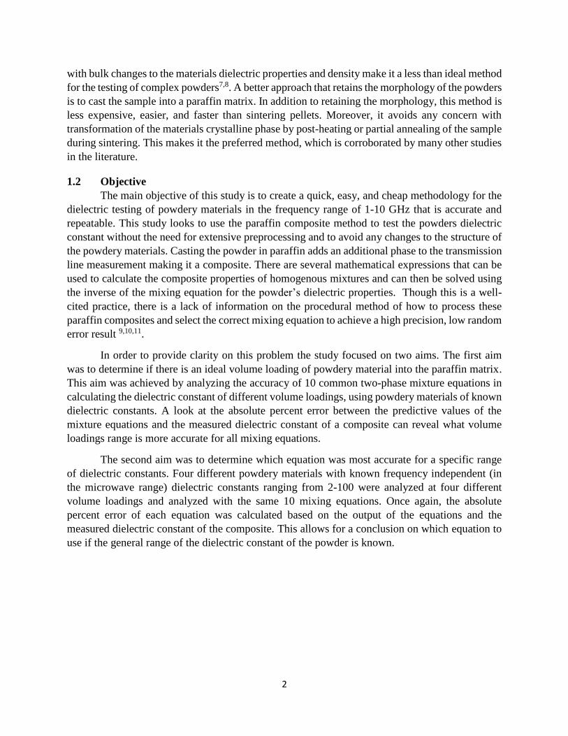
ionosphere12. Microwaves fall within the inferred and radio waves in the electromagnetic spectrum
which is shown in Figure 2.113.
Figure 2.1: Electromagnetic spectrum with a visualization of the visible spectrum shown as a
subset of electromagnetic radiation13.
Microwaves are used in a wide variety of applications such as point-to-point
communication links, wireless networks, microwave radio relay networks, radar, medical
diathermy, cancer treatments, remote sensing, satellite communication, spacecraft communication,
radio astronomy, spectroscopy, industrial heating, collision avoidance systems, particle
accelerators, garage door openers and keyless entry systems, and for cooking food in microwave
ovens14.
Microwaves consist of electromagnetic waves made up of two components, an electric
field and a magnetic field. Microwaves are synchronized oscillations of the electric and magnetic
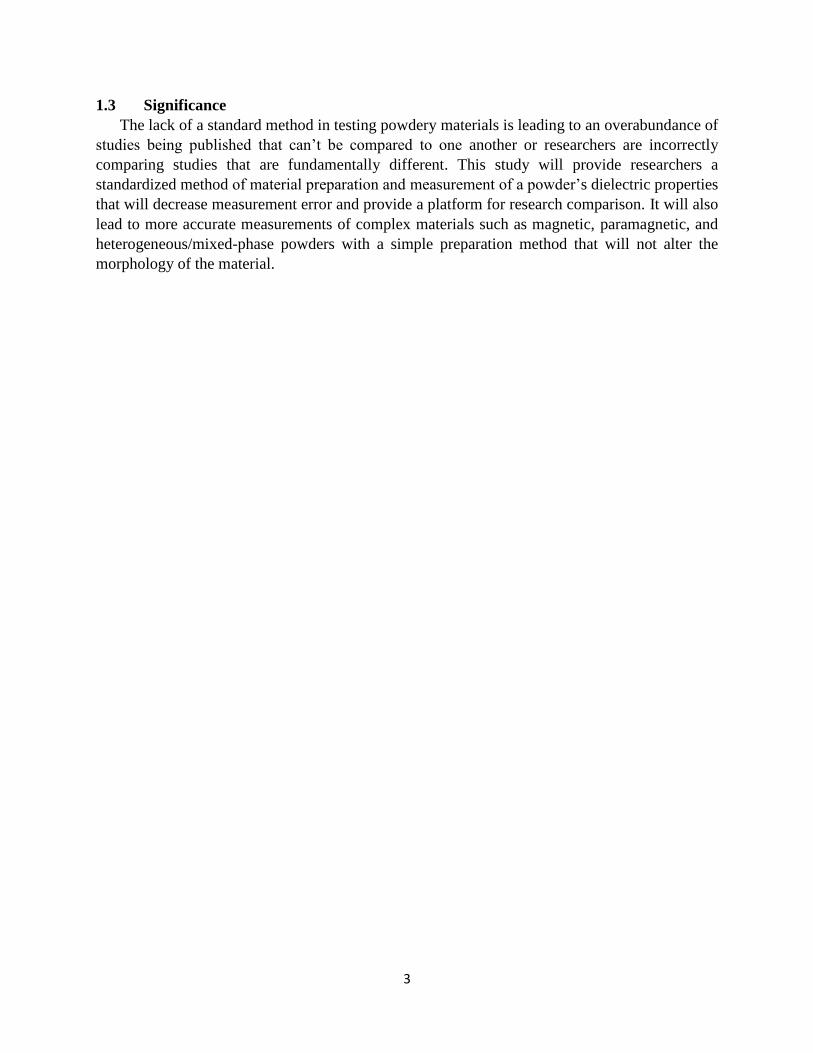
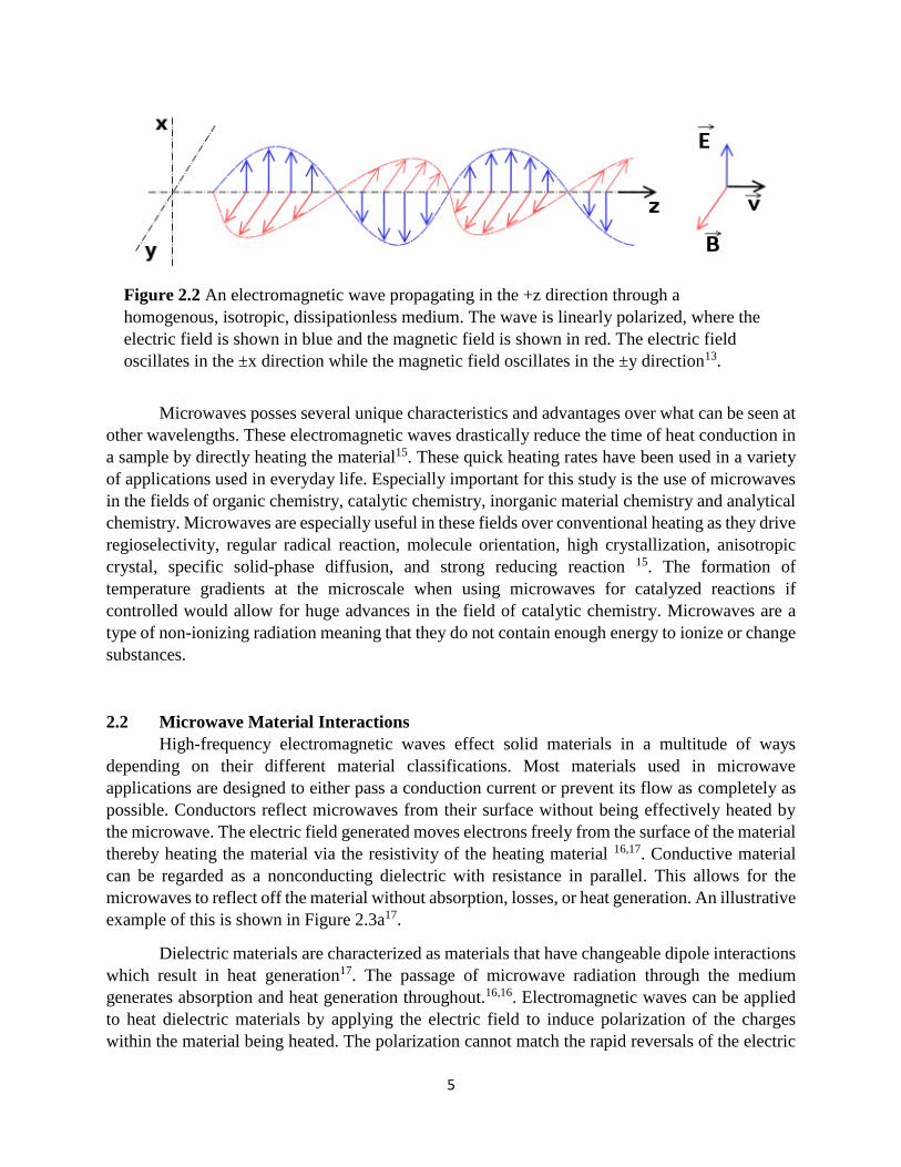
fields both of which propagate at the speed of light. These two waves are commonly perpendicular
to one another and to the direction of the energy, with this perpendicular wave propagation forming
a transverse wave, this is shown in Figure 2.213.
5
Microwaves posses several unique characteristics and advantages over what can be seen at
other wavelengths. These electromagnetic waves drastically reduce the time of heat conduction in
a sample by directly heating the material15. These quick heating rates have been used in a variety
of applications used in everyday life. Especially important for this study is the use of microwaves
in the fields of organic chemistry, catalytic chemistry, inorganic material chemistry and analytical
chemistry. Microwaves are especially useful in these fields over conventional heating as they drive
regioselectivity, regular radical reaction, molecule orientation, high crystallization, anisotropic
crystal, specific solid-phase diffusion, and strong reducing reaction 15. The formation of
temperature gradients at the microscale when using microwaves for catalyzed reactions if
controlled would allow for huge advances in the field of catalytic chemistry. Microwaves are a
type of non-ionizing radiation meaning that they do not contain enough energy to ionize or change
substances.
2.2 Microwave Material Interactions
High-frequency electromagnetic waves effect solid materials in a multitude of ways
depending on their different material classifications. Most materials used in microwave
applications are designed to either pass a conduction current or prevent its flow as completely as
possible. Conductors reflect microwaves from their surface without being effectively heated by
the microwave. The electric field generated moves electrons freely from the surface of the material
thereby heating the material via the resistivity of the heating material 16,17. Conductive material
can be regarded as a nonconducting dielectric with resistance in parallel. This allows for the
microwaves to reflect off the material without absorption, losses, or heat generation. An illustrative
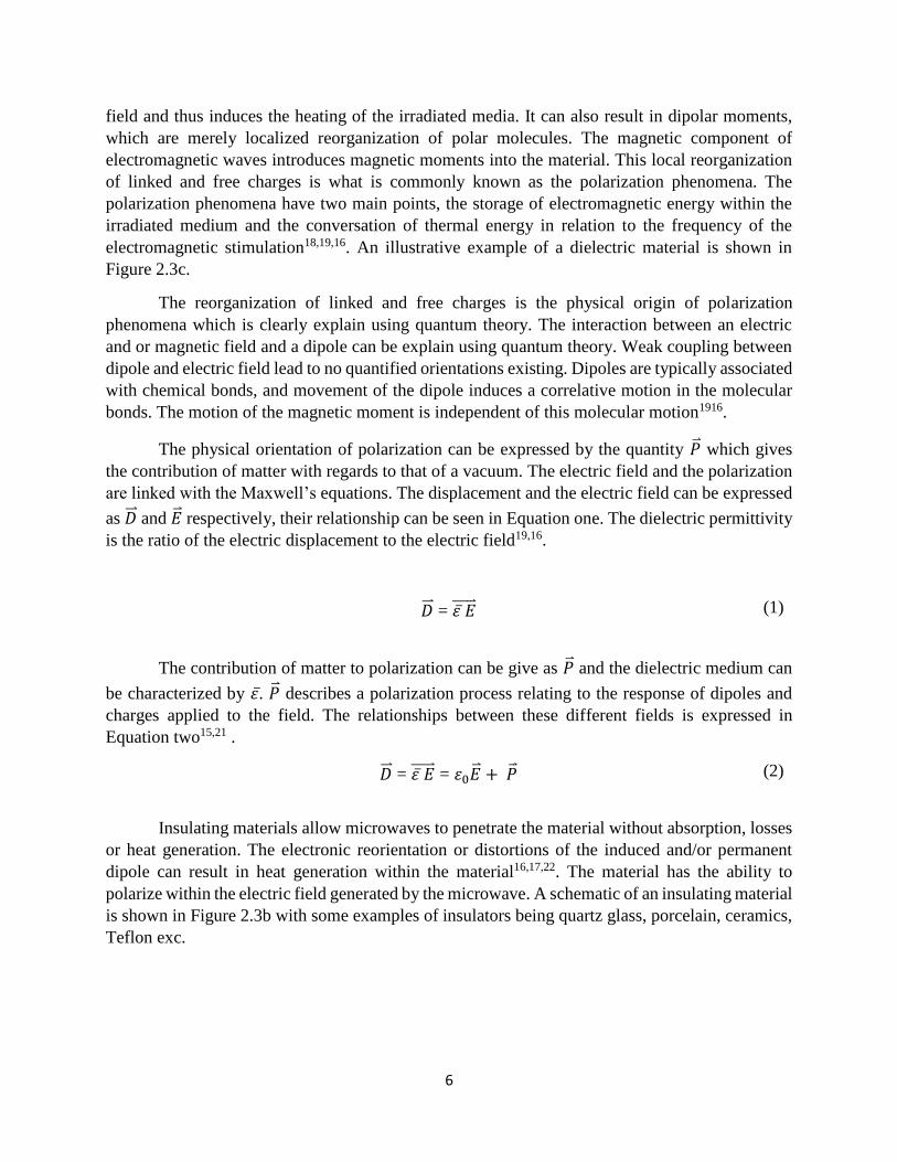
example of this is shown in Figure 2.3a17.
Dielectric materials are characterized as materials that have changeable dipole interactions
which result in heat generation17. The passage of microwave radiation through the medium
generates absorption and heat generation throughout.16,16. Electromagnetic waves can be applied
to heat dielectric materials by applying the electric field to induce polarization of the charges
within the material being heated. The polarization cannot match the rapid reversals of the electric
Figure 2.2 An electromagnetic wave propagating in the +z direction through a
homogenous, isotropic, dissipationless medium. The wave is linearly polarized, where the
electric field is shown in blue and the magnetic field is shown in red. The electric field
oscillates in the ±x direction while the magnetic field oscillates in the ±y direction13.
6
field and thus induces the heating of the irradiated media. It can also result in dipolar moments,
which are merely localized reorganization of polar molecules. The magnetic component of
electromagnetic waves introduces magnetic moments into the material. This local reorganization
of linked and free charges is what is commonly known as the polarization phenomena. The
polarization phenomena have two main points, the storage of electromagnetic energy within the
irradiated medium and the conversation of thermal energy in relation to the frequency of the
electromagnetic stimulation18,19,16. An illustrative example of a dielectric material is shown in
Figure 2.3c.
The reorganization of linked and free charges is the physical origin of polarization
phenomena which is clearly explain using quantum theory. The interaction between an electric
and or magnetic field and a dipole can be explain using quantum theory. Weak coupling between
dipole and electric field lead to no quantified orientations existing. Dipoles are typically associated
with chemical bonds, and movement of the dipole induces a correlative motion in the molecular
bonds. The motion of the magnetic moment is independent of this molecular motion1916.
The physical orientation of polarization can be expressed by the quantity �⃑� which gives
the contribution of matter with regards to that of a vacuum. The electric field and the polarization
are linked with the Maxwell’s equations. The displacement and the electric field can be expressed
as �⃑⃑� and �⃑� respectively, their relationship can be seen in Equation one. The dielectric permittivity
is the ratio of the electric displacement to the electric field19,16.
�⃑⃑� = 휀 ̅𝐸⃑⃑ ⃑⃑ ⃑ (1)
The contribution of matter to polarization can be give as �⃑� and the dielectric medium can
be characterized by 휀.̅ �⃑� describes a polarization process relating to the response of dipoles and
charges applied to the field. The relationships between these different fields is expressed in
Equation two15,21 .
�⃑⃑� = 휀 ̅𝐸⃑⃑ ⃑⃑ ⃑ = 휀0�⃑� + �⃑� (2)
Insulating materials allow microwaves to penetrate the material without absorption, losses
or heat generation. The electronic reorientation or distortions of the induced and/or permanent
dipole can result in heat generation within the material16,17,22. The material has the ability to
polarize within the electric field generated by the microwave. A schematic of an insulating material
is shown in Figure 2.3b with some examples of insulators being quartz glass, porcelain, ceramics,
Teflon exc.
7
2.2.1 Permittivity
The capacitance encountered in the formation of an electric field of a medium is denoted
as the absolute permittivity. This can be expressed as the amount of charge needed to generate one
unit of electric flux in the medium being studied. Permittivity in essence is a materials ability to
store an electric field in the polarization of the medium19. A material’s dielectric medium usually
is expressed as the relative permittivity of the material, this term is commonly called the dielectric
constant in literature2,23. It can be expressed as kappa κ which is the ratio of the absolute
permittivity to the electric constant. Dielectric constant is not typically constant, it varies with
position in the medium, the frequency of the field applied, humidity, temperature, and other
parameters. In a nonlinear medium the dielectric constant can vary with the strength of the applied
electric field19.
κ = 휀𝑟 = 𝜀
𝜀0 (3)
The dielectric constant is directly proportional to the electric susceptibility χ, which is a
measurement of how easily a dielectric polarizes in response to an electric field. The relation of
these terms is given in equations 4 and 5.
χ = κ - 1 (4)
휀 = 휀𝑟휀0 = (1+ χ) 휀0 (5)
The two main points of wave-matter interactions can be expressed by the two components
of the dielectric constant.
휀 = 휀′ − 𝑗휀′′ = 휀0휀𝑟′ − 𝑗휀0휀𝑟
′′ (6)
Where 휀′, 휀′′, 휀𝑟′ , and 휀𝑟
′′ are the real and imaginary parts of the complex dielectric
permittivity and the real and imaginary parts of the relative complex dielectric permittivity. The
ability of a material to store electromagnetic energy is expressed as the real part and the thermal
Figure 2.3: Subfigure a: electrical conducting material, subfigure b: insulating material,
subfigure c: dielectric material17.
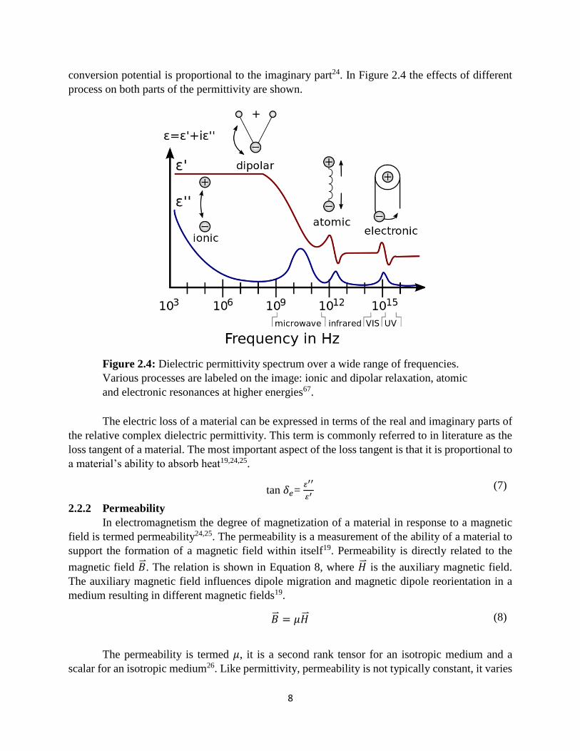
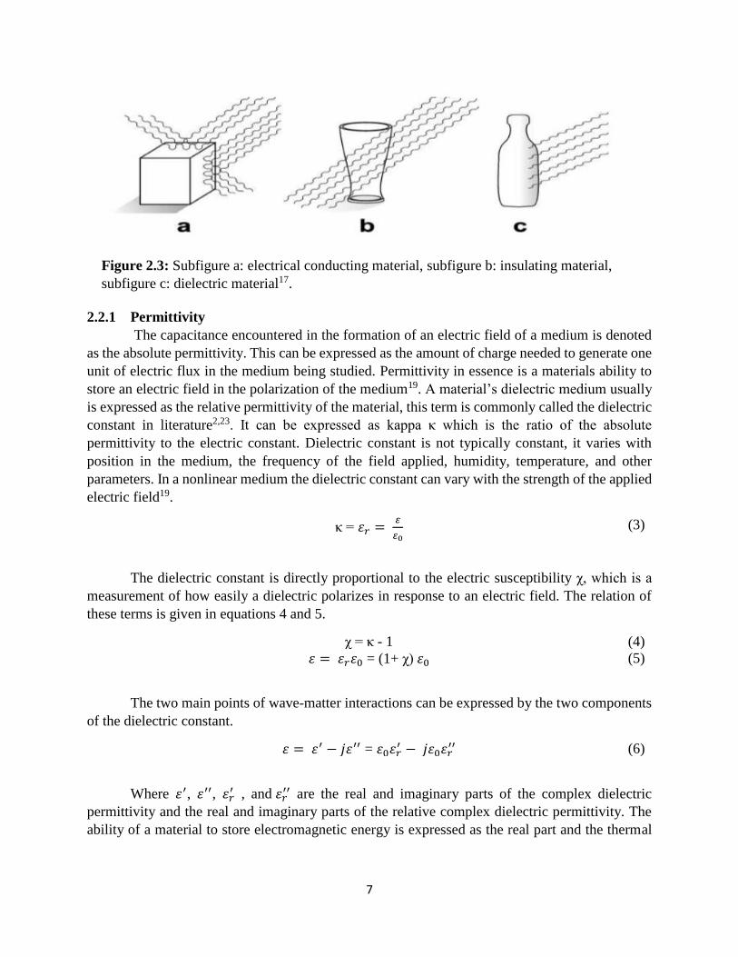
8
conversion potential is proportional to the imaginary part24. In Figure 2.4 the effects of different
process on both parts of the permittivity are shown.
The electric loss of a material can be expressed in terms of the real and imaginary parts of
the relative complex dielectric permittivity. This term is commonly referred to in literature as the
loss tangent of a material. The most important aspect of the loss tangent is that it is proportional to
a material’s ability to absorb heat19,24,25.
tan 𝛿𝑒= 𝜀′′
𝜀′ (7)
2.2.2 Permeability
In electromagnetism the degree of magnetization of a material in response to a magnetic
field is termed permeability24,25. The permeability is a measurement of the ability of a material to
support the formation of a magnetic field within itself19. Permeability is directly related to the
magnetic field �⃑� . The relation is shown in Equation 8, where �⃑⃑� is the auxiliary magnetic field.
The auxiliary magnetic field influences dipole migration and magnetic dipole reorientation in a
medium resulting in different magnetic fields19.
�⃑� = 𝜇�⃑⃑� (8)
The permeability is termed 𝜇, it is a second rank tensor for an isotropic medium and a
scalar for an isotropic medium26. Like permittivity, permeability is not typically constant, it varies
Figure 2.4: Dielectric permittivity spectrum over a wide range of frequencies.
Various processes are labeled on the image: ionic and dipolar relaxation, atomic
and electronic resonances at higher energies67.

9
with position in the medium, the frequency of the field applied, humidity, temperature, and other
parameters. In a nonlinear medium the dielectric constant can vary with the strength of the applied
magnetic field27,28,29.
Like permittivity, there is a relative permeability that is merely the ratio of the permeability
of a specific medium to the permeability of a free space. The relative permeability is directly
related to the magnetic susceptibility19.
𝜇𝑟 = 𝜇
𝜇0 (9)
𝜒𝑚 = 𝜇𝑟 − 1 (10)
The relative permeability has both a real and imaginary portion just like that of the
dielectric constant. Where the real part is the magnetic permeability and the imaginary part is the
magnetic loss. The ratio of which is a measure of how much power is lost in a material versus how
much is stored19. The losses of a material are induced by the domain walls and from the electron
spin resonance12,19,30. The material can be placed at the magnetic field maxima in order to allow
for maximum absorption of microwave energy12,19,30.
𝜇 = 𝜇′ − 𝑗𝜇′′ = 𝜇0𝜇𝑟′ − 𝑗𝜇0𝜇𝑟
′′ (11)
tan 𝛿𝑚= 𝜇′′
𝜇′ (12)
2.2.3 Microscopic, Local and Macroscopic Fields
When a semi-infinite medium has an electromagnetic field applied the material will show
effects from the particle back-reaction field and the applied field19. This results in charges and
spins inside the medium which react with the local fields but not directly with the applied field. In
the case of a dielectric material, the surface-charge dipole-depolarization fields that oppose the
applied field will change the macroscopic and local fields in the material when interacting with an
electromagnetic field19. This relationship grows more complex as consideration is made for the
time-dependent high-frequency fields. In this circumstance the dipole orientations and thus the
electromagnetic fields can be affected by a number of factors, including depolarization,
demagnetization, thermal expansion, exchange, and anisotropy interactions12,19,30.
When modeling the relationships between the applied, macroscopic, local, and microscopic
fields a special attention must be payed to where the fields originate from and their interactions
with one another. External charges generate the applied fields, while the macroscopic fields are
merely the averaged quantities in the medium. The macroscopic fields can be implicitly defined
through the constitutive relationships with boundary conditions.
2.2.4 Local Electromagnetic Fields in Materials
The effective local field is commonly defined as the Lorentz field in literature, where the
Lorentz field is defined as the field in a cavity that is varved out of a material around a specific
10
site. The local field for a Lorentz spherical cavity can be defined as the sum of the applied (𝐸𝑎),
depolarization (𝐸𝑑𝑒𝑝), Lorentz (𝐸𝐿𝑜𝑟𝑒𝑛𝑡𝑧) , and atomic fields (𝐸𝑎𝑡𝑜𝑚) as shown in Equation
1316,19,30.
𝐸𝑙 = 𝐸𝑎 + 𝐸𝑑𝑒𝑝 + 𝐸𝐿𝑜𝑟𝑒𝑛𝑡𝑧 + 𝐸𝑎𝑡𝑜𝑚 (13)
Where for a cubic lattice in the sphere the applied field can be related to the macroscopic
field and polarization by Equation 1416.
𝐸𝑙 = 𝐸 +
1
3휀0𝑃
(14)
This polarization field (P) for a molecule is expressed as a function of the local field (E), which
can in turn be expressed as a function of the macroscopic field. These relationships can be seen in
equations 15 and 1616.
𝑝 ≈ 𝛼𝐸𝑙 (15)
𝐸𝑙 = 𝛽𝐸 (16)
The relationship is between the fields is difficult to calculate, this is due to the local field’s
relationship to the macroscopic field, the polarizabilities, permittivity, and permeability absorb
parts of the local field.
2.3 Measurement Models for Material Properties
2.3.1 Transmission/Reflection measurement techniques for lossy materials
The characterization of microwave material interactions can be defined as a mathematical
model, where the waves that are reflected and transmitted through the material at a certain
frequency are measured. In a transmission/reflection (TR) measurement, a material is placed into
a waveguide or coaxial line and subjected to a microwave with a known frequency26. The material
reflects part of that wave while allowing for some of it to pass through. The study of this effect
revels the specimen’s dielectric properties. The reflection and transmission data are known as
scattering data. The scattering data must be solved using the electromagnetic boundary-value
problem in order to determine the materials properties26.
2.3.2 Scattering Parameters
Scattering parameters (S-parameters) are a type of small-signal AC commonly used to
characterize RF components. S-parameters establish small-signal characteristics of a device at a
specific bias and temperature31. They are measured by making the measuring device impeded
between a 50-ohm load and a source, drastically reducing the chance of oscillations to occur. S-
parameters have the distinct advantage of not varying in magnitude at points along a lossless
transmission line because they are traveling waves not terminal voltages31. A signal wave for a
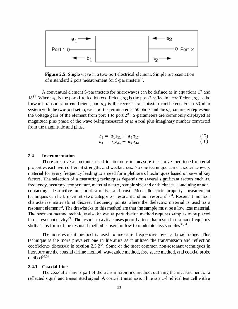
two-port electrical-element is represented in Figure 2.5, where a1 is the wave into port 1, a2 is the
wave into port 2, b1 is the wave out of port 1, and b2 is the wave out of port 2.
11
A conventual element S-parameters for microwaves can be defined as in equations 17 and
1818. Where s11 is the port-1 reflection coefficient, s22 is the port-2 reflection coefficient, s21 is the
forward transmission coefficient, and s12 is the reverse transmission coefficient. For a 50 ohm
system with the two-port setup, each port is terminated at 50 ohms and the s21 parameter represents
the voltage gain of the element from port 1 to port 232. S-parameters are commonly displayed as
magnitude plus phase of the wave being measured or as a real plus imaginary number converted
from the magnitude and phase.
𝑏1 = 𝑎1𝑠11 + 𝑎2𝑎12 (17)
𝑏2 = 𝑎1𝑠21 + 𝑎2𝑎22 (18)
2.4 Instrumentation
There are several methods used in literature to measure the above-mentioned material
properties each with different strengths and weaknesses. No one technique can characterize every
material for every frequency leading to a need for a plethora of techniques based on several key
factors. The selection of a measuring techniques depends on several significant factors such as,
frequency, accuracy, temperature, material nature, sample size and or thickness, containing or non-
contacting, destructive or non-destructive and cost. Most dielectric property measurement
techniques can be broken into two categories; resonant and non-resonant33,34. Resonant methods
characterize materials at discreet frequency points where the dielectric material is used as a
resonant element33. The drawbacks to this method are that the sample must be a low loss material.
The resonant method technique also known as perturbation method requires samples to be placed
into a resonant cavity33,. The resonant cavity causes perturbations that result in resonant frequency
shifts. This form of the resonant method is used for low to moderate loss samples33,34.
The non-resonant method is used to measure frequencies over a broad range. This
technique is the more prevalent one in literature as it utilized the transmission and reflection
coefficients discussed in section 2.3.233. Some of the most common non-resonant techniques in
literature are the coaxial airline method, waveguide method, free space method, and coaxial probe
method33,34.
2.4.1 Coaxial Line
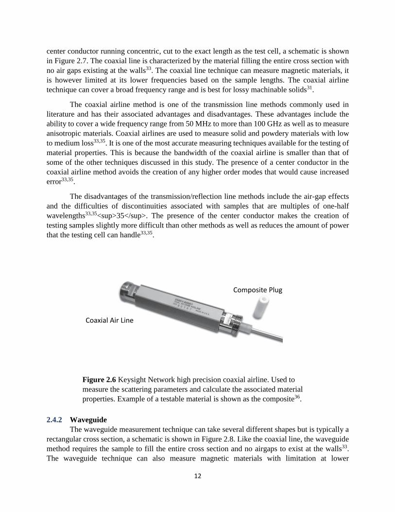
The coaxial airline is part of the transmission line method, utilizing the measurement of a
reflected signal and transmitted signal. A coaxial transmission line is a cylindrical test cell with a
Figure 2.5: Single wave in a two-port electrical-element. Simple representation
of a standard 2 port measurement for S-parameters32.
12
center conductor running concentric, cut to the exact length as the test cell, a schematic is shown
in Figure 2.7. The coaxial line is characterized by the material filling the entire cross section with
no air gaps existing at the walls33. The coaxial line technique can measure magnetic materials, it
is however limited at its lower frequencies based on the sample lengths. The coaxial airline
technique can cover a broad frequency range and is best for lossy machinable solids31.
The coaxial airline method is one of the transmission line methods commonly used in
literature and has their associated advantages and disadvantages. These advantages include the
ability to cover a wide frequency range from 50 MHz to more than 100 GHz as well as to measure
anisotropic materials. Coaxial airlines are used to measure solid and powdery materials with low
to medium loss33,35. It is one of the most accurate measuring techniques available for the testing of
material properties. This is because the bandwidth of the coaxial airline is smaller than that of
some of the other techniques discussed in this study. The presence of a center conductor in the
coaxial airline method avoids the creation of any higher order modes that would cause increased
error33,35.
The disadvantages of the transmission/reflection line methods include the air-gap effects
and the difficulties of discontinuities associated with samples that are multiples of one-half
wavelengths33,35<sup>35</sup>. The presence of the center conductor makes the creation of
testing samples slightly more difficult than other methods as well as reduces the amount of power
that the testing cell can handle33,35.
2.4.2 Waveguide
The waveguide measurement technique can take several different shapes but is typically a
rectangular cross section, a schematic is shown in Figure 2.8. Like the coaxial line, the waveguide
method requires the sample to fill the entire cross section and no airgaps to exist at the walls33.
The waveguide technique can also measure magnetic materials with limitation at lower
Figure 2.6 Keysight Network high precision coaxial airline. Used to
measure the scattering parameters and calculate the associated material
properties. Example of a testable material is shown as the composite36.
Composite Plug
Coaxial Air Line
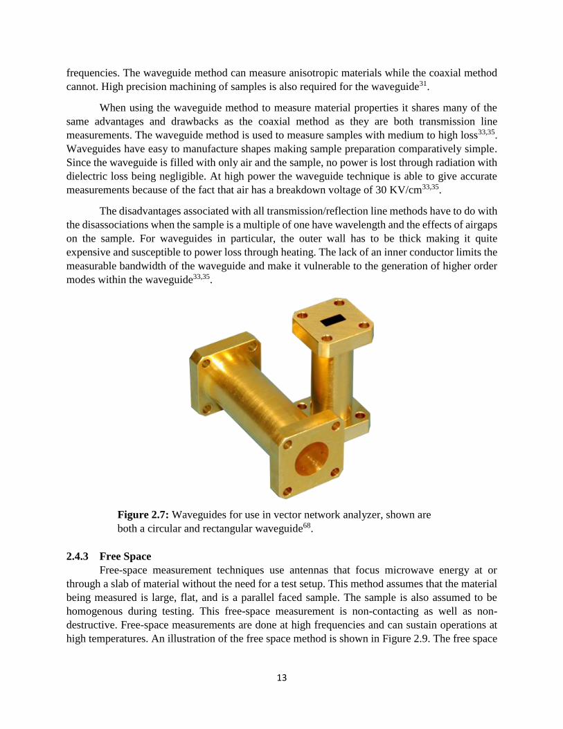
13
frequencies. The waveguide method can measure anisotropic materials while the coaxial method
cannot. High precision machining of samples is also required for the waveguide31.
When using the waveguide method to measure material properties it shares many of the
same advantages and drawbacks as the coaxial method as they are both transmission line
measurements. The waveguide method is used to measure samples with medium to high loss33,35.
Waveguides have easy to manufacture shapes making sample preparation comparatively simple.
Since the waveguide is filled with only air and the sample, no power is lost through radiation with
dielectric loss being negligible. At high power the waveguide technique is able to give accurate
measurements because of the fact that air has a breakdown voltage of 30 KV/cm33,35.
The disadvantages associated with all transmission/reflection line methods have to do with
the disassociations when the sample is a multiple of one have wavelength and the effects of airgaps
on the sample. For waveguides in particular, the outer wall has to be thick making it quite
expensive and susceptible to power loss through heating. The lack of an inner conductor limits the
measurable bandwidth of the waveguide and make it vulnerable to the generation of higher order
modes within the waveguide33,35.
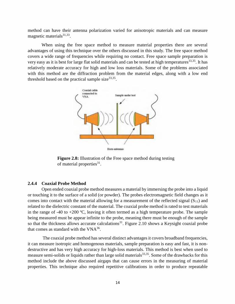
2.4.3 Free Space
Free-space measurement techniques use antennas that focus microwave energy at or
through a slab of material without the need for a test setup. This method assumes that the material
being measured is large, flat, and is a parallel faced sample. The sample is also assumed to be
homogenous during testing. This free-space measurement is non-contacting as well as non-
destructive. Free-space measurements are done at high frequencies and can sustain operations at
high temperatures. An illustration of the free space method is shown in Figure 2.9. The free space
Figure 2.7: Waveguides for use in vector network analyzer, shown are
both a circular and rectangular waveguide68.
14
method can have their antenna polarization varied for anisotropic materials and can measure
magnetic materials31,33.
When using the free space method to measure material properties there are several
advantages of using this technique over the others discussed in this study. The free space method
covers a wide range of frequencies while requiring no contact. Free space sample preparation is
very easy as it is best for large flat solid materials and can be tested at high temperatures33,35. It has
relatively moderate accuracy for high and low loss materials. Some of the problems associated
with this method are the diffraction problem from the material edges, along with a low end
threshold based on the practical sample size33,35.
2.4.4 Coaxial Probe Method
Open ended coaxial probe method measures a material by immersing the probe into a liquid
or touching it to the surface of a solid (or powder). The probes electromagnetic field changes as it
comes into contact with the material allowing for a measurement of the reflected signal (S11) and
related to the dielectric constant of the material. The coaxial probe method is rated to test materials
in the range of -40 to +200 ºC, leaving it often termed as a high temperature probe. The sample
being measured must be appear infinite to the probe, meaning there must be enough of the sample
so that the thickness allows accurate calculations31. Figure 2.10 shows a Keysight coaxial probe
that comes as standard with the VNA36.
The coaxial probe method has several distinct advantages it covers broadband frequencies,
it can measure isotropic and homogenous materials, sample preparation is easy and fast, it is non-
destructive and has very high accuracy for high-loss materials. This method is best when used to
measure semi-solids or liquids rather than large solid materials33,35. Some of the drawbacks for this
method include the above discussed airgaps that can cause errors in the measuring of material
properties. This technique also required repetitive calibrations in order to produce repeatable
Figure 2.8: Illustration of the Free space method during testing
of material properties31.
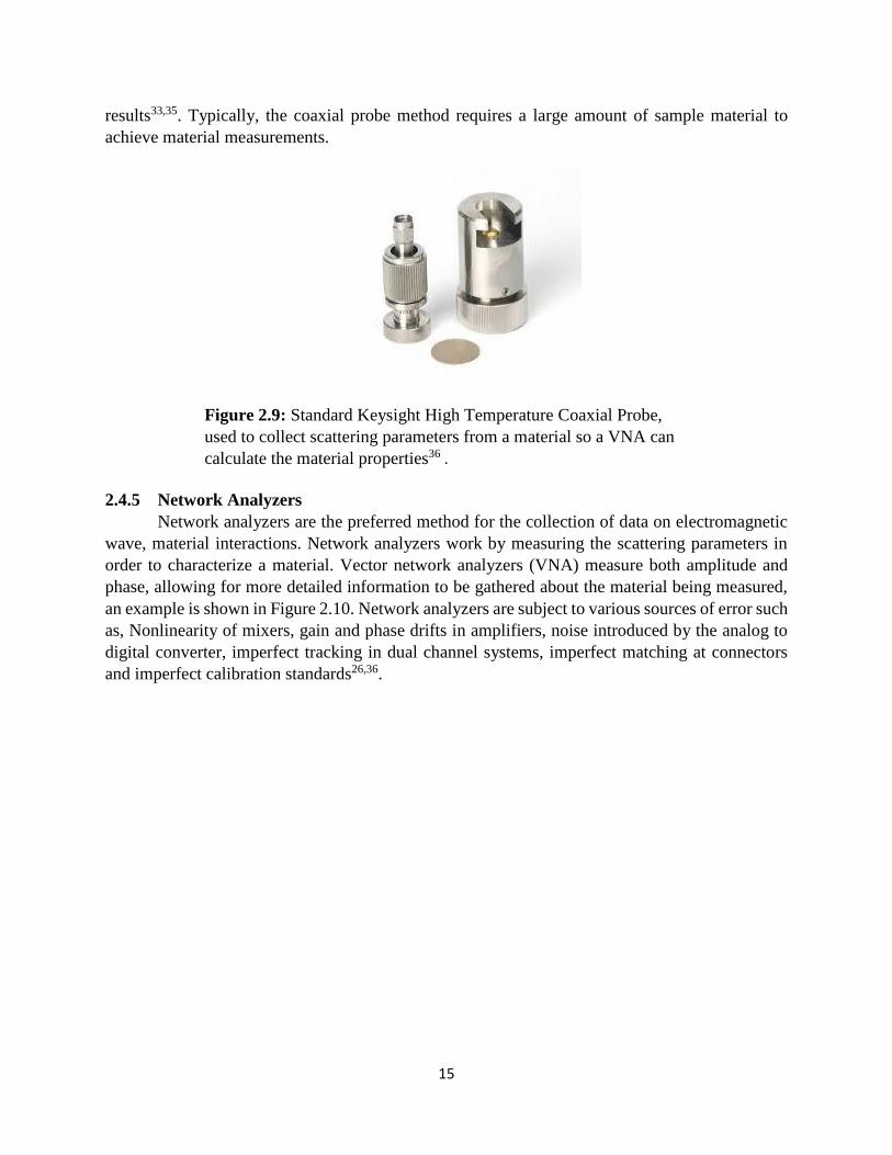
15
results33,35. Typically, the coaxial probe method requires a large amount of sample material to
achieve material measurements.
2.4.5 Network Analyzers
Network analyzers are the preferred method for the collection of data on electromagnetic
wave, material interactions. Network analyzers work by measuring the scattering parameters in
order to characterize a material. Vector network analyzers (VNA) measure both amplitude and
phase, allowing for more detailed information to be gathered about the material being measured,
an example is shown in Figure 2.10. Network analyzers are subject to various sources of error such
as, Nonlinearity of mixers, gain and phase drifts in amplifiers, noise introduced by the analog to
digital converter, imperfect tracking in dual channel systems, imperfect matching at connectors
and imperfect calibration standards26,36.
Figure 2.9: Standard Keysight High Temperature Coaxial Probe,
used to collect scattering parameters from a material so a VNA can
calculate the material properties36 .
16
2.5 Error
2.5.1 Random Uncertainties and Error
In transmission/reflection measurement techniques there are several different types of
error, one of them being random uncertainties of the calibration and from the specimen itself. The
three main types of random uncertainties and error sources typically related to
transmission/reflection measurements are errors in measuring the magnitude and phase of the
scattering parameters, error in specimen length and error in reference plane positions26. To
counteract this problem a differential uncertainty analysis can be applied to both s11 and s21
separately. For both s11 and s21 the dominate uncertainty is the phase, with longer specimens having
less uncertainty. It has been found in literature that at higher frequencies S-parameters have larger
uncertainties in phase26.
2.5.2 Systematic Uncertainties
The other type of error associated with transmission/reflection measurements is systematic
uncertainties. These uncertainties can be broken down into several main types, gaps between the
specimen and specimen holder and specimen holder dimensional variations and line losses and
connector mismatch26. There are standard equations in literature that are made to handle the first
type of uncertainties for gaps around the specimen37,38. Along with airgaps other systematic
uncertainties include short-circuit and waveguide wall imperfections and losses26. Waveguide
losses can be corrected with by taking a measurement of an empty waveguide and calculating the
appropriate correction factor or attenuation coefficient. For airgaps additional measurements using
a resonator of the same material in the frequency band being measured will determine the required
gap in the correction formula.
2.5.3 Corrections to Data
With the many possible errors associated with dielectric measurement testing and the
difficulty of data collection, corrections must be made once a measurement has been obtained. The
Figure 2.10: Keysight Network Analyzer part of the vector network analyzer
family of machinery. Used primarily to measure the scattering parameters and
calculate the associated material properties. VNA’s are used for many of the
different techniques mentioned in the following sections36.

17
corrections must account for the systematic uncertainties and if possible the random uncertainties
and error. Known uncertainties associated with transmission/reflection measurements are airgaps
around the sample, wall imperfections, and losses. Airgap corrections are most important when
considering the coaxial method of testing with particular emphasis on the center conductor26. For
both coaxial and waveguide method, airgap correction are particularly important in whichever
region has the strongest electromagnetic field 37,38. Both waveguides and coaxial lines at ambient
temperature will experience some power loss because they are not perfectly conducting. The
different propagation modes will be attenuated to some degree because of this power loss 26.
2.6 Permeability and Permittivity Calculations
2.6.1 Nicolson-Ross-Weir
The most widely used method for calculating permittivity and permeability from S-
parameters is the Nicolson, Ross, Weir method (NRW)39,29. This method is applicable over the
range of 100 MHz to 18 GHz when using a computer-controlled network analyzer. However it is
subject to singularities when the specimen length is a multiple of one-half wavelength in the
material26. This is especially prevalent for low-loss materials as it is impossible to measure the
phase of S11 accurately. NRW takes measurements in the frequency domain rather than the time
domain24,25 which avoids the need of using a Fourier transform to calculate permittivity and
permeability. The NRW method works for both waveguides and coaxial lines using discrete
frequencies in less than 20 kHz steps29.
2.6.2 Nicolson-Ross-Weir Polynomial Method
The NRW polynomial method is an iterative technique to fit material properties to a
polynomial. This method increments the method of the polynomial until the difference between S-
parameters calculated from the polynomial and the measured S-parameters are less than the
expected system performance. This method can also be done using a user specified maximum
order for the polynomial23,40.
2.6.3 NIST Iterative Solution
For a general iterative solution if the material being tested has a known length and reference
plane it is possible to use an iterative solution to solve for the permittivity and permeability. Using
various linear combinations of the scattering equations and solving them iteratively will result in
a stable solution for permetivity26. This iterative method however can be unstable when solving
for both permittivity and permeability, with integrals of one-half wavelength causing the instability
due to the TEM mode resonance. The NIST iterative solution is only suitable for permittivity
calculations as it assumes the permeability is equal to one. A solution is obtained using a Newton-
Raphson’s root finding method35. The common inaccuracy peaks associated with the NRW method
are avoid when using the NIST iterative method, making it suitable for long samples and low loss
materials35. However, a disadvantage of this method is the need for a good initial guess.
2.6.4 NIST Non-Iterative
The NIST non-iterative method like the iterative method is only applicable for permittivity
calculations as it also assumes the permeability of one. The non-iterative method is similar to the
NRW method but with a different formulation of equation based on the assumption of permeability
of one. Unlike NRW this method is stable over the whole range of frequencies for any sample
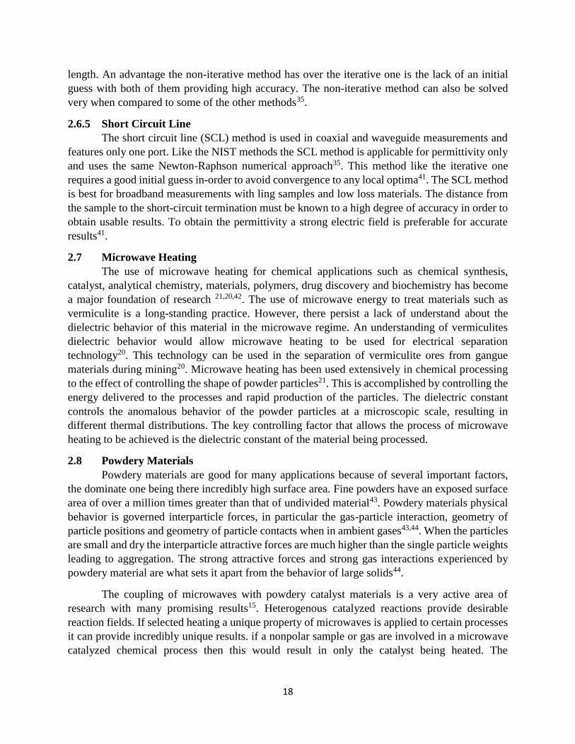
18
length. An advantage the non-iterative method has over the iterative one is the lack of an initial
guess with both of them providing high accuracy. The non-iterative method can also be solved
very when compared to some of the other methods35.
2.6.5 Short Circuit Line
The short circuit line (SCL) method is used in coaxial and waveguide measurements and
features only one port. Like the NIST methods the SCL method is applicable for permittivity only
and uses the same Newton-Raphson numerical approach35. This method like the iterative one
requires a good initial guess in-order to avoid convergence to any local optima41. The SCL method
is best for broadband measurements with ling samples and low loss materials. The distance from
the sample to the short-circuit termination must be known to a high degree of accuracy in order to
obtain usable results. To obtain the permittivity a strong electric field is preferable for accurate
results41.
2.7 Microwave Heating
The use of microwave heating for chemical applications such as chemical synthesis,
catalyst, analytical chemistry, materials, polymers, drug discovery and biochemistry has become
a major foundation of research 21,20,42. The use of microwave energy to treat materials such as
vermiculite is a long-standing practice. However, there persist a lack of understand about the
dielectric behavior of this material in the microwave regime. An understanding of vermiculites
dielectric behavior would allow microwave heating to be used for electrical separation
technology20. This technology can be used in the separation of vermiculite ores from gangue
materials during mining20. Microwave heating has been used extensively in chemical processing
to the effect of controlling the shape of powder particles21. This is accomplished by controlling the
energy delivered to the processes and rapid production of the particles. The dielectric constant
controls the anomalous behavior of the powder particles at a microscopic scale, resulting in
different thermal distributions. The key controlling factor that allows the process of microwave
heating to be achieved is the dielectric constant of the material being processed.
2.8 Powdery Materials
Powdery materials are good for many applications because of several important factors,
the dominate one being there incredibly high surface area. Fine powders have an exposed surface
area of over a million times greater than that of undivided material43. Powdery materials physical
behavior is governed interparticle forces, in particular the gas-particle interaction, geometry of
particle positions and geometry of particle contacts when in ambient gases43,44. When the particles
are small and dry the interparticle attractive forces are much higher than the single particle weights
leading to aggregation. The strong attractive forces and strong gas interactions experienced by
powdery material are what sets it apart from the behavior of large solids44.
The coupling of microwaves with powdery catalyst materials is a very active area of
research with many promising results15. Heterogenous catalyzed reactions provide desirable
reaction fields. If selected heating a unique property of microwaves is applied to certain processes
it can provide incredibly unique results. if a nonpolar sample or gas are involved in a microwave
catalyzed chemical process then this would result in only the catalyst being heated. The
19
understanding of heterogenous powdery catalyst can greatly increase the possible reactions used
in a multitude of fields.
2.9 Specimen Preparations for Powdery Material
2.9.1 Sintering
Powdery sample preparation for many different procedures requiring a process called
sintering to form the desired shape and material characteristics. Sintering involves heating a
powder at high temperatures any typically also involves pressing a powder into a desired
temperature. Sintering effects many different physical attributes of powders including porosity and
grain size resulting in changes to hardness, yield stress, compressive strength, and wear
resistance45. For most powders as sintering temperature increases grain size increases while
porosity is reduced45, this makes finding a balance between them to maximize mechanical behavior
an important factor in powder processing. It has also been found in literature that sintering has a
direct effect on density and lattice structure46. These effects can have repercussions on the
dielectric constant and other parameters affecting them in unknown and uncontrollable ways.
Sandi et al. shows a direct correlation between sintering temperature and dielectric constant47.
Sintering can help in many processes to form the desired shape, but sintering can also have
unknown and unpredictable consequences on internal material parameters. As figure 2.11 shows
sintering has a drastic effect on particle morphology48, this is especially true for multi-phase
powders like catalyst. These changes in morphology as a result of sintering would render most
catalyst useless.
2.9.2 Pressing
Pressing uses pressure to form powder into the desired shape, either using hot or cold
pressing49. Hot pressing involves packing a powder into the desired shape at an elevated
temperature. This technique is usually coupled with sintering to achieve the desired shape. Cold
pressing is accomplished by applying pressure on a loose column of powders in a closed die to
form a compact powder50. It can be further classified into two more types of pressing, axial
pressing or isostatic pressing. The effects of pressure on powders is highly dependent on their
particle size, shape, composition, and size distribution49. Pressing powders has several drawbacks
Figure 2.11: (a) Alumina pellet with individual grains, (b) well sintered pellet
with defined cleavage plans at 1580 ºC48.
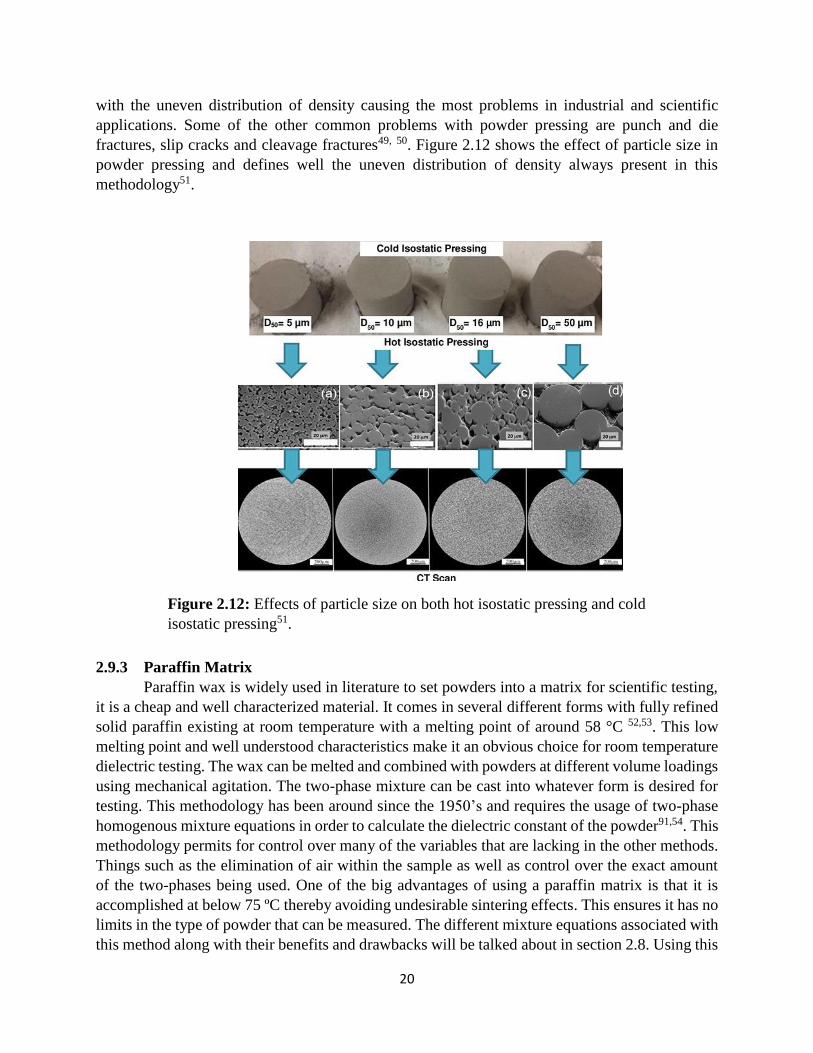
20
with the uneven distribution of density causing the most problems in industrial and scientific
applications. Some of the other common problems with powder pressing are punch and die
fractures, slip cracks and cleavage fractures49, 50. Figure 2.12 shows the effect of particle size in
powder pressing and defines well the uneven distribution of density always present in this
methodology51.
2.9.3 Paraffin Matrix
Paraffin wax is widely used in literature to set powders into a matrix for scientific testing,
it is a cheap and well characterized material. It comes in several different forms with fully refined
solid paraffin existing at room temperature with a melting point of around 58 °C 52,53. This low
melting point and well understood characteristics make it an obvious choice for room temperature
dielectric testing. The wax can be melted and combined with powders at different volume loadings
using mechanical agitation. The two-phase mixture can be cast into whatever form is desired for
testing. This methodology has been around since the 1950’s and requires the usage of two-phase
homogenous mixture equations in order to calculate the dielectric constant of the powder91,54. This
methodology permits for control over many of the variables that are lacking in the other methods.
Things such as the elimination of air within the sample as well as control over the exact amount
of the two-phases being used. One of the big advantages of using a paraffin matrix is that it is
accomplished at below 75 ºC thereby avoiding undesirable sintering effects. This ensures it has no
limits in the type of powder that can be measured. The different mixture equations associated with
this method along with their benefits and drawbacks will be talked about in section 2.8. Using this
Figure 2.12: Effects of particle size on both hot isostatic pressing and cold
isostatic pressing51.

21
methodology allows for the reduction of unknown variables resulting in more accurate test results
then the other methods presented in this paper.
2.10 Mixture equations for Two Phase Homogenous Composites
The process of determining the dielectric constant is a complex process with no exact
solution existing. There are several equations in literature that attempt to take the dielectric
constant of two different materials and predict their combined dielectric constant. These equations
are of use in the paraffin composite methodology as they can be set to solve for the dielectric
constant of the constitutive material with the composites dielectric constant being experimentally
tested. These equations are almost exclusively based on only four variables, the dielectric constant
of the powder and its volume loading, the dielectric constant of the inclusion matrix and its volume
loading and the dielectric constant of the two-phase composite. The EMT mixture equation
discussed in section 2.8.8 has an additional variable of a shape factor constant. The equations all
aim to predict the behavior of the dipole-dipole interactions between the different phases of the
materials, with varying degrees of success19. The difficulty in predicting the dielectric constant of
a two-phase homogenous composite lies in the fact that no exact solution existing for the
electrostatic problem in a random heterogenous geometry1. This study focuses on measuring the
dielectric constant of the two-phase mixture and back-calculating the dielectric constant of
powders dielectric constant.
2.10.1 Parallel Mixing Equation
One of the standard equations for predicting the dielectric constant of a two-phase
homogenous composite is the parallel mixing equation. Equation 19 shows the parallel mixing
equation also sometimes called the linear law, it is part of a family of predictive equations called
the power law family. This formula is abdicable if the theoretical configuration of the mixture is
formed of plates or other types of inclusion where no depolarization is induced 55. This mixture
equation is made to mimic that of a parallel plate capacitor. The following sections use the same
nomenclature where 휀𝑚𝑖𝑥, 휀𝑚, and 휀𝑝 stand for the dielectric constant of the mixture composite,
matrix material (paraffin), and powdery material respectively. 𝑉𝑝 is the volume loading of the
powder and 𝑉𝑚 is the volume loading of the paraffin1.
휀𝑚𝑖𝑥 = 𝑉𝑝휀𝑝 + 𝑉𝑚휀𝑚 (19)
2.10.2 Series Mixing Equation
Another equation for predicting the dielectric constant of a composite is the series mixing
equation. Equation 20 is setup so that the dielectric constant of the components behave like that of
a series capacitor54.
(휀𝑚𝑖𝑥)−1 = 𝑉𝑝(휀𝑝)
−1 + 𝑉𝑚(휀𝑚𝑖𝑥)−1 (20)

22
2.10.3 Logarithmic Mixing Equation
The Logarithmic mixture equation can be shown to be derive from the famous Maxwell-
Garnet equations56. It is another empirical equation that aims to predict the behavior of two
intermixed dielectric constants. The formula was obtained by further assuming a random
distribution of shapes and orientations for each component enabling the charge density at any
position to be replaced by the mean charge density of the mixture56.
ln(휀𝑚𝑖𝑥) = 𝑉𝑝ln (휀𝑝) + 𝑉𝑚ln (휀𝑚) (21)
2.10.4 Lichtenecker Mixing Equation
The Lichtenecker mixing equation is another of the power-law family of equations. This
equation averages the logarithms of the permittivity’s in order to mathematically predict the
dielectric constant of the mixture55.
휀𝑚𝑖𝑥 = 휀𝑝
𝑉𝑝 ∗ 휀𝑚𝑉𝑚 (22)
2.10.5 Looyenga Mixing Equation
The Looyenga mixture equation is one of the differential mixing models available in
literate. It attempts to mathematically predict the internal microstructure interaction between
dipoles. These equations are derived based on differential analysis rather than on first principle
calculations. This equation is considered to be similar to the Bruggeman family of equations
because of the symmetry between matrix and inclusion1.
휀𝑚𝑖𝑥1/3 = 𝑉𝑚휀𝑚
1/3 + 𝑉𝑝휀𝑝1/3
(23)
2.10.6 Birchak Mixing Equation
The Birchak mixing equation is also part of the power-law family of equations were the
permittivity is averaged by volume weights. For this formula the square roots of each components
permittivity add up to the square root of the mixtures permittivity. This mathematical model also
can be used to state that the refractive index of a mixture’s nonmagnetic gases is the volume
average of the indices of each component a useful tool in optical physics1.
휀𝑚𝑖𝑥1/2 = 𝑉𝑚휀𝑚
1/2 + 𝑉𝑝휀𝑝1/2
(24)
2.10.7 Poon-Shin Mixing Equation
The Poon-Shin Mixture equation is derived from the polarization of each inclusion related
to the electric field along with the electrical displacement as a function of electrical field and
polarization. The Poon-Shin model revolves around the idea of the displacement field as a function
of a single particle’s sum forces. Those forces are broken down to the medium and the polarization
of the particles that are embedded in the medium5754. This equation is desired for when the
23
dielectric constant of the inclusion particle is greater than that of the matrix material, for our
application this translates to 휀𝑝 < 휀𝑚57.
휀𝑚𝑖𝑥 = 휀𝑚 [1 + 𝑉𝑃(
휀𝑝
휀𝑚− 1)
𝑉𝑃 + (𝑉𝑚3 ) [
휀𝑝
휀𝑚𝑉𝑚 + 𝑉𝑝 + 2]
]
(25)
2.10.8 Effective Medium Theory Mixing Equation
The Effective Medium Theory mixing equation (EMT) is one of the Maxwell-Garnet
family of equations. It is an algebraic formula were the mixtures dielectric constant is calculated
as a function of the constituent permittivity’s their volume fraction and a shape factor denoted n.
This model attempts to idealize the geometry and model the microstructure using simple forms30,54.
The EMT mixing equation is designed to include first-order scattering effects of the inclusions.
The contribution to the imaginary part of the effective permittivity is estimated by calculating the
energy that the electric dipoles radiate30,55. Where n acts in the equation as a depolarization factor.
휀𝑚𝑖𝑥 = 휀𝑚 [1 +
𝑉𝑝(휀𝑝 − 휀𝑚)
휀𝑚 + 𝑛𝑉𝑝(휀𝑝 − 휀𝑚)]
(26)
2.10.9 Maxwell-Garnet Mixing Equation
The Maxwell-Garnet Mixing equation is one of the oldest and most popular mixture
equations for two-phase dielectric composites. The equation was derived based on ignoring the
associated density fluctuations about a mean value and instead focusing on the dipole character of
scattering1,58. This approach can be used to include the finite-size effects of scattering, with the
main limitation being the lack of discrimination between two random media. This is especially
true when the media has the same density of scattering but have different statistical
distributions1,55,59,30. It is commonly claimed that weak particle interaction is a condition of the
Maxwell-Garnet theory.
휀𝑚𝑖𝑥 = 휀𝑚 + 3 ∗ 𝑉𝑝휀𝑚 (
휀𝑝 − 휀𝑚
휀𝑝 + 2휀𝑚 − 𝑉𝑝(휀𝑝 − 휀𝑚))
(27)
2.10.10 Jayasundere-Smith Mixing Equation
The Jayasundere-Smith Mixing equation was derived in order to predict the dielectric
constant of binary piezoelectric0-3 composites. Jaysundere and Smith derived their expression by
modifying Kerner’s expression. Which focused on the interactions of isolated dielectric spheres in
a dielectric continuum. The system that this equation is design to handle is composed of
piezoelectric sphere with a dielectric sphere dispersed in a constant medium. Where the spheres
dielectric is always greater than that of the medium60.
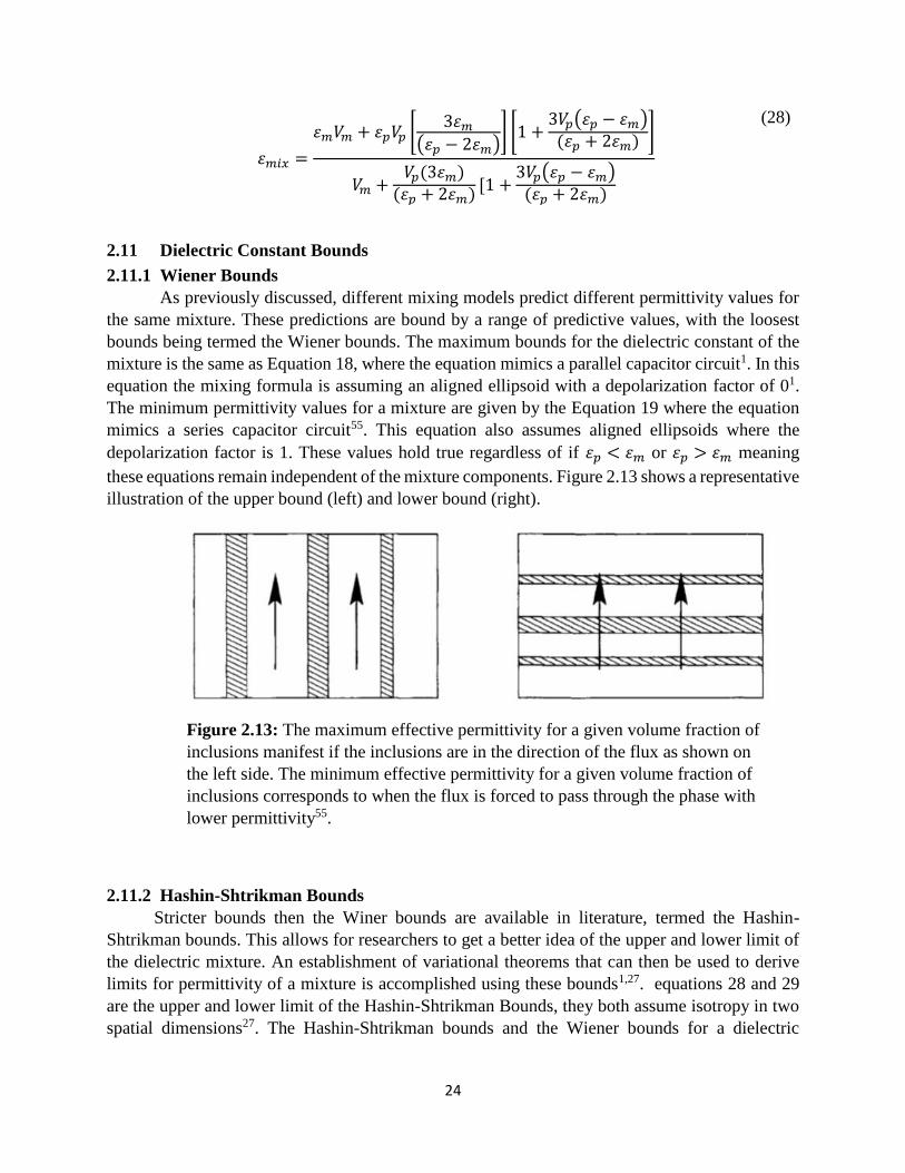
24
휀𝑚𝑖𝑥 =
휀𝑚𝑉𝑚 + 휀𝑝𝑉𝑝 [3휀𝑚
(휀𝑝 − 2휀𝑚)] [1 +
3𝑉𝑝(휀𝑝 − 휀𝑚)(휀𝑝 + 2휀𝑚)
]
𝑉𝑚 +𝑉𝑝(3휀𝑚)
(휀𝑝 + 2휀𝑚)[1 +
3𝑉𝑝(휀𝑝 − 휀𝑚)(휀𝑝 + 2휀𝑚)
(28)
2.11 Dielectric Constant Bounds
2.11.1 Wiener Bounds
As previously discussed, different mixing models predict different permittivity values for
the same mixture. These predictions are bound by a range of predictive values, with the loosest
bounds being termed the Wiener bounds. The maximum bounds for the dielectric constant of the
mixture is the same as Equation 18, where the equation mimics a parallel capacitor circuit1. In this
equation the mixing formula is assuming an aligned ellipsoid with a depolarization factor of 01.
The minimum permittivity values for a mixture are given by the Equation 19 where the equation
mimics a series capacitor circuit55. This equation also assumes aligned ellipsoids where the
depolarization factor is 1. These values hold true regardless of if 휀𝑝 < 휀𝑚 or 휀𝑝 > 휀𝑚 meaning
these equations remain independent of the mixture components. Figure 2.13 shows a representative
illustration of the upper bound (left) and lower bound (right).
2.11.2 Hashin-Shtrikman Bounds
Stricter bounds then the Winer bounds are available in literature, termed the Hashin-
Shtrikman bounds. This allows for researchers to get a better idea of the upper and lower limit of
the dielectric mixture. An establishment of variational theorems that can then be used to derive
limits for permittivity of a mixture is accomplished using these bounds1,27. equations 28 and 29
are the upper and lower limit of the Hashin-Shtrikman Bounds, they both assume isotropy in two
spatial dimensions27. The Hashin-Shtrikman bounds and the Wiener bounds for a dielectric
Figure 2.13: The maximum effective permittivity for a given volume fraction of
inclusions manifest if the inclusions are in the direction of the flux as shown on
the left side. The minimum effective permittivity for a given volume fraction of
inclusions corresponds to when the flux is forced to pass through the phase with
lower permittivity55.
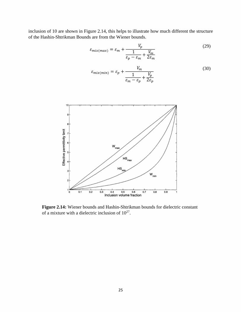
25
inclusion of 10 are shown in Figure 2.14, this helps to illustrate how much different the structure
of the Hashin-Shtrikman Bounds are from the Wiener bounds.
휀𝑚𝑖𝑥(𝑚𝑎𝑥) = 휀𝑚 +
𝑉𝑝1
휀𝑝 − 휀𝑚+
𝑉𝑚2휀𝑚
(29)
휀𝑚𝑖𝑥(𝑚𝑖𝑛) = 휀𝑝 +
𝑉𝑚1
휀𝑚 − 휀𝑝+
𝑉𝑝2휀𝑝
(30)
Figure 2.14: Wiener bounds and Hashin-Shtrikman bounds for dielectric constant
of a mixture with a dielectric inclusion of 1027.
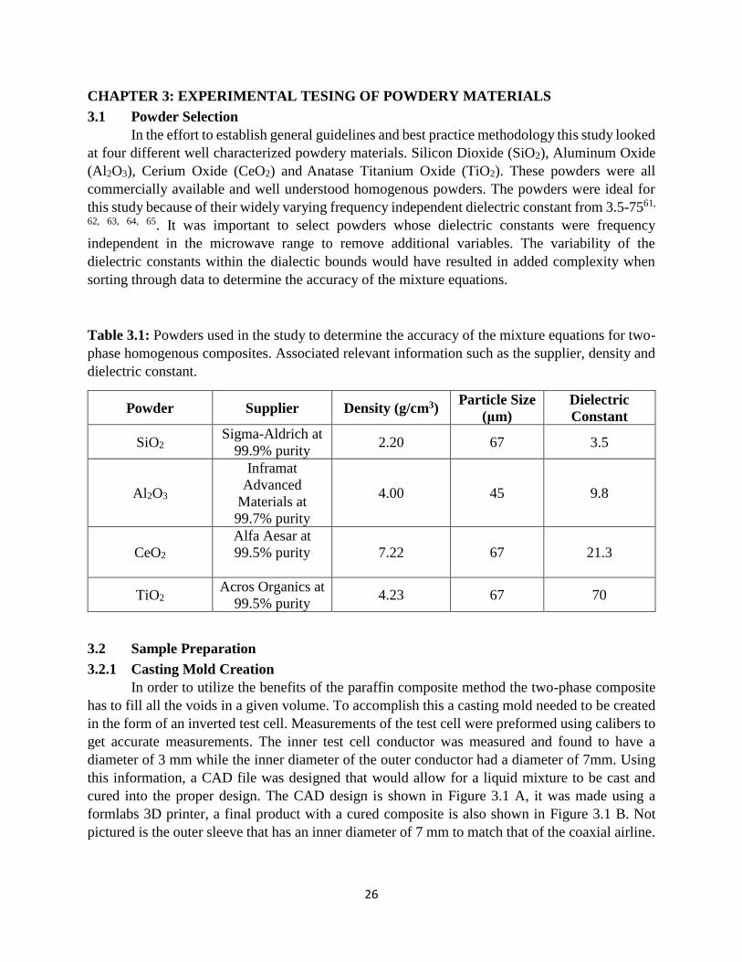
26
CHAPTER 3: EXPERIMENTAL TESING OF POWDERY MATERIALS
3.1 Powder Selection
In the effort to establish general guidelines and best practice methodology this study looked
at four different well characterized powdery materials. Silicon Dioxide (SiO2), Aluminum Oxide
(Al2O3), Cerium Oxide (CeO2) and Anatase Titanium Oxide (TiO2). These powders were all
commercially available and well understood homogenous powders. The powders were ideal for
this study because of their widely varying frequency independent dielectric constant from 3.5-7561,
62, 63, 64, 65. It was important to select powders whose dielectric constants were frequency
independent in the microwave range to remove additional variables. The variability of the
dielectric constants within the dialectic bounds would have resulted in added complexity when
sorting through data to determine the accuracy of the mixture equations.
Table 3.1: Powders used in the study to determine the accuracy of the mixture equations for two-
phase homogenous composites. Associated relevant information such as the supplier, density and
dielectric constant.
Powder Supplier Density (g/cm3) Particle Size
(μm)
Dielectric
Constant
SiO2 Sigma-Aldrich at
99.9% purity 2.20 67 3.5
Al2O3
Inframat
Advanced
Materials at
99.7% purity
4.00 45 9.8
CeO2
Alfa Aesar at
99.5% purity
7.22 67 21.3
TiO2 Acros Organics at
99.5% purity 4.23 67 70
3.2 Sample Preparation
3.2.1 Casting Mold Creation
In order to utilize the benefits of the paraffin composite method the two-phase composite
has to fill all the voids in a given volume. To accomplish this a casting mold needed to be created
in the form of an inverted test cell. Measurements of the test cell were preformed using calibers to
get accurate measurements. The inner test cell conductor was measured and found to have a
diameter of 3 mm while the inner diameter of the outer conductor had a diameter of 7mm. Using
this information, a CAD file was designed that would allow for a liquid mixture to be cast and
cured into the proper design. The CAD design is shown in Figure 3.1 A, it was made using a
formlabs 3D printer, a final product with a cured composite is also shown in Figure 3.1 B. Not
pictured is the outer sleeve that has an inner diameter of 7 mm to match that of the coaxial airline.
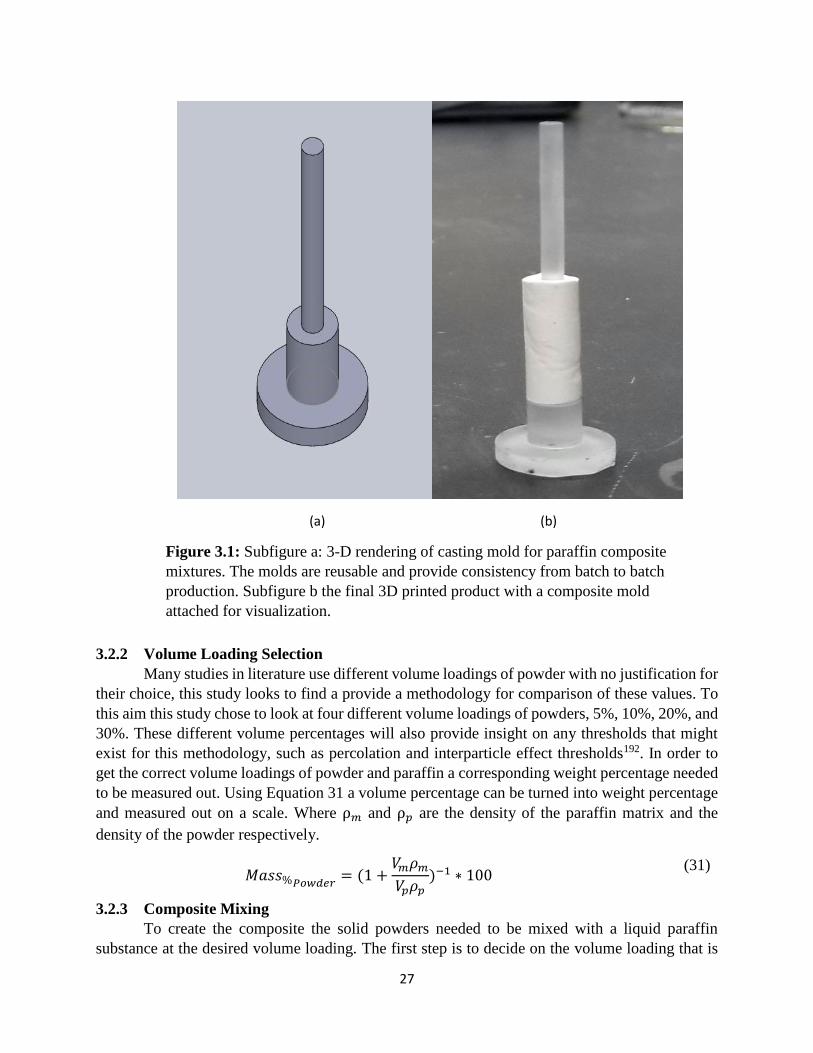
27
3.2.2 Volume Loading Selection
Many studies in literature use different volume loadings of powder with no justification for
their choice, this study looks to find a provide a methodology for comparison of these values. To
this aim this study chose to look at four different volume loadings of powders, 5%, 10%, 20%, and
30%. These different volume percentages will also provide insight on any thresholds that might
exist for this methodology, such as percolation and interparticle effect thresholds192. In order to
get the correct volume loadings of powder and paraffin a corresponding weight percentage needed
to be measured out. Using Equation 31 a volume percentage can be turned into weight percentage
and measured out on a scale. Where ρ𝑚 and ρ𝑝 are the density of the paraffin matrix and the
density of the powder respectively.
𝑀𝑎𝑠𝑠%𝑃𝑜𝑤𝑑𝑒𝑟
= (1 +𝑉𝑚𝜌𝑚
𝑉𝑝𝜌𝑝)−1 ∗ 100
(31)
3.2.3 Composite Mixing
To create the composite the solid powders needed to be mixed with a liquid paraffin
substance at the desired volume loading. The first step is to decide on the volume loading that is
(a) (b)
Figure 3.1: Subfigure a: 3-D rendering of casting mold for paraffin composite
mixtures. The molds are reusable and provide consistency from batch to batch
production. Subfigure b the final 3D printed product with a composite mold
attached for visualization.
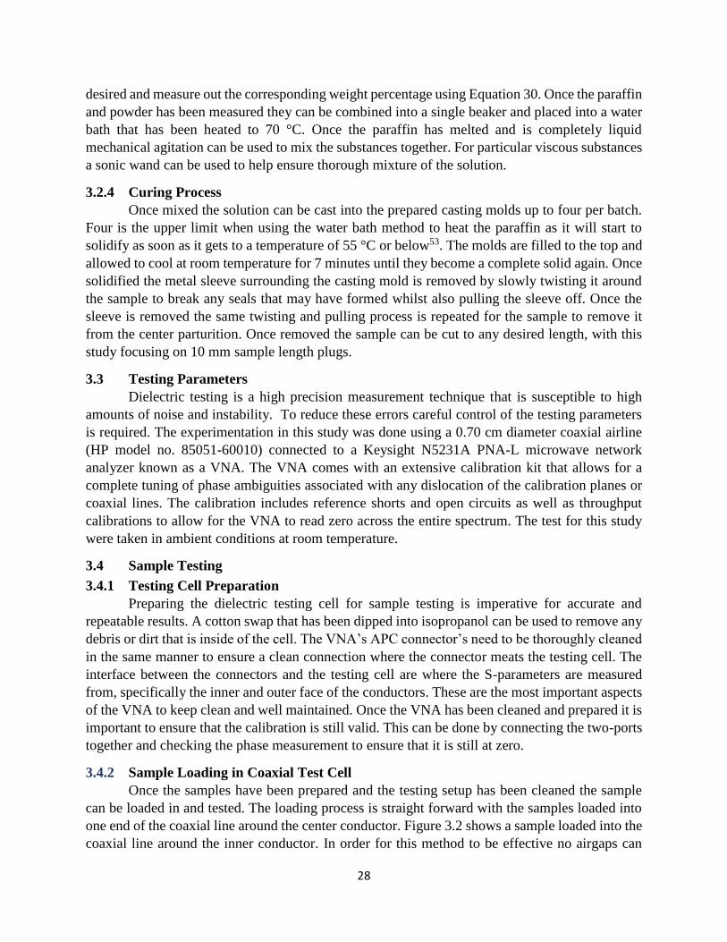
28
desired and measure out the corresponding weight percentage using Equation 30. Once the paraffin
and powder has been measured they can be combined into a single beaker and placed into a water
bath that has been heated to 70 °C. Once the paraffin has melted and is completely liquid
mechanical agitation can be used to mix the substances together. For particular viscous substances
a sonic wand can be used to help ensure thorough mixture of the solution.
3.2.4 Curing Process
Once mixed the solution can be cast into the prepared casting molds up to four per batch.
Four is the upper limit when using the water bath method to heat the paraffin as it will start to
solidify as soon as it gets to a temperature of 55 °C or below53. The molds are filled to the top and
allowed to cool at room temperature for 7 minutes until they become a complete solid again. Once
solidified the metal sleeve surrounding the casting mold is removed by slowly twisting it around
the sample to break any seals that may have formed whilst also pulling the sleeve off. Once the
sleeve is removed the same twisting and pulling process is repeated for the sample to remove it
from the center parturition. Once removed the sample can be cut to any desired length, with this
study focusing on 10 mm sample length plugs.
3.3 Testing Parameters
Dielectric testing is a high precision measurement technique that is susceptible to high
amounts of noise and instability. To reduce these errors careful control of the testing parameters
is required. The experimentation in this study was done using a 0.70 cm diameter coaxial airline
(HP model no. 85051-60010) connected to a Keysight N5231A PNA-L microwave network
analyzer known as a VNA. The VNA comes with an extensive calibration kit that allows for a
complete tuning of phase ambiguities associated with any dislocation of the calibration planes or
coaxial lines. The calibration includes reference shorts and open circuits as well as throughput
calibrations to allow for the VNA to read zero across the entire spectrum. The test for this study
were taken in ambient conditions at room temperature.
3.4 Sample Testing
3.4.1 Testing Cell Preparation
Preparing the dielectric testing cell for sample testing is imperative for accurate and
repeatable results. A cotton swap that has been dipped into isopropanol can be used to remove any
debris or dirt that is inside of the cell. The VNA’s APC connector’s need to be thoroughly cleaned
in the same manner to ensure a clean connection where the connector meats the testing cell. The
interface between the connectors and the testing cell are where the S-parameters are measured
from, specifically the inner and outer face of the conductors. These are the most important aspects
of the VNA to keep clean and well maintained. Once the VNA has been cleaned and prepared it is
important to ensure that the calibration is still valid. This can be done by connecting the two-ports
together and checking the phase measurement to ensure that it is still at zero.
3.4.2 Sample Loading in Coaxial Test Cell
Once the samples have been prepared and the testing setup has been cleaned the sample
can be loaded in and tested. The loading process is straight forward with the samples loaded into
one end of the coaxial line around the center conductor. Figure 3.2 shows a sample loaded into the
coaxial line around the inner conductor. In order for this method to be effective no airgaps can

29
exist between the sample and the inner or outer conductor. It is also important to ensure no debris
from the paraffin composite are blocking the testing interfaces. Straight smooth edges will allow
for more accurate measurements of the S-parameters. Once the sample is loaded compressed air
can be used to remove any excess debris from the testing setup.
3.4.3 Testing Initiation
Once the sample has been loaded and is securely in place with no debris a testing procedure
can be conducted. Both ends of the airline need to be securely fashioned to the APC connectors in
the same orientation that the calibration was performed at. In Figure 3.3 a loaded test cell is shown
that is prepared for testing. Once the test cell has been loaded a mathematical model (section 2.3)
needs to be selected that transform the S-parameters into the permittivity and permeability. This
study used the NRW polynomial method to calculate the permittivity of the composite plugs in
order to avoid any discontinuities associated with one half wavelength measurements. Once the
model has been selected, the user must define the testing range and number of measurement points.
For this study the dielectric properties from 1-10 GHz were investigated using 1601 equally spaced
points. Once the model has been selected the VNA will begin measuring and computing until all
the designated measurements have been achieved.
Figure 3.2: Paraffin-powder material composite plug loaded into the precision
airline. The plug fills all the space between the center electrode and the outer
electrode to ensure no airgaps exist.
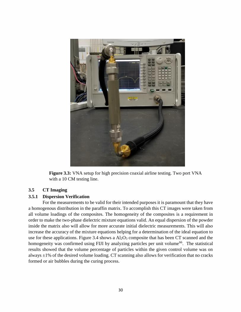
30
3.5 CT Imaging
3.5.1 Dispersion Verification
For the measurements to be valid for their intended purposes it is paramount that they have
a homogenous distribution in the paraffin matrix. To accomplish this CT images were taken from
all volume loadings of the composites. The homogeneity of the composites is a requirement in
order to make the two-phase dielectric mixture equations valid. An equal dispersion of the powder
inside the matrix also will allow for more accurate initial dielectric measurements. This will also
increase the accuracy of the mixture equations helping for a determination of the ideal equation to
use for these applications. Figure 3.4 shows a Al2O3 composite that has been CT scanned and the
homogeneity was confirmed using FIJI by analyzing particles per unit volume66. The statistical
results showed that the volume percentage of particles within the given control volume was on
always ±1% of the desired volume loading. CT scanning also allows for verification that no cracks
formed or air bubbles during the curing process.
Figure 3.3: VNA setup for high precision coaxial airline testing. Two port VNA
with a 10 CM testing line.
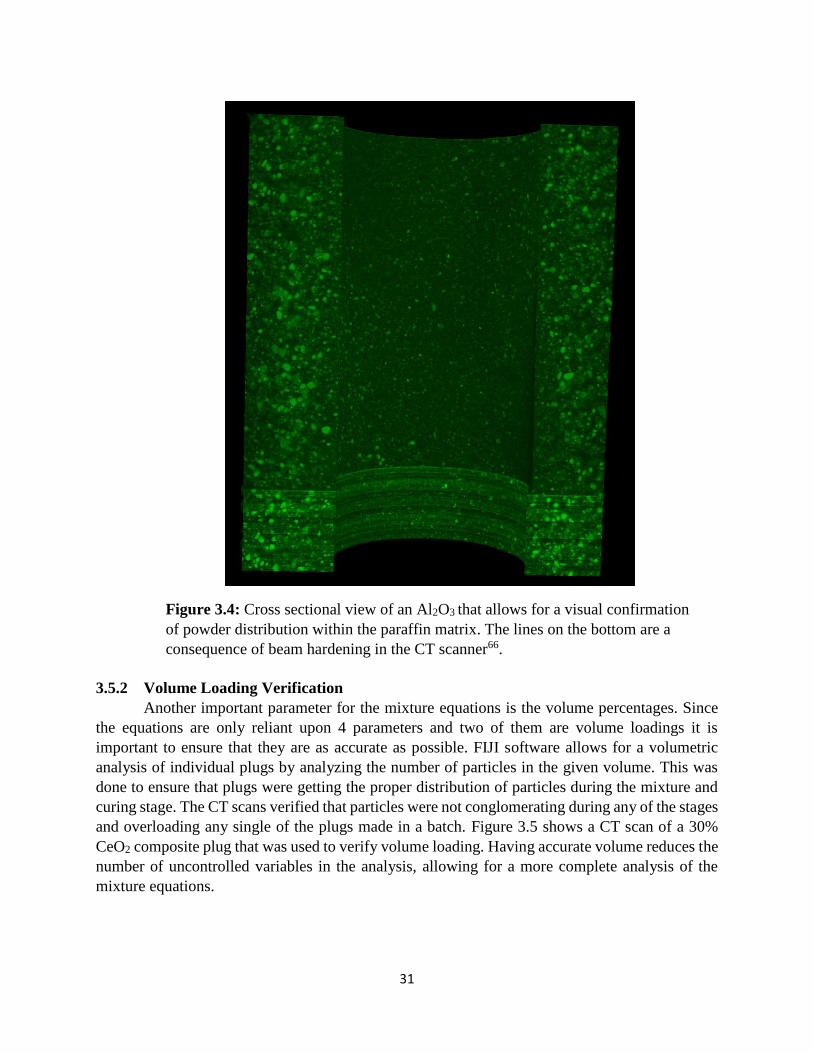
31
3.5.2 Volume Loading Verification
Another important parameter for the mixture equations is the volume percentages. Since
the equations are only reliant upon 4 parameters and two of them are volume loadings it is
important to ensure that they are as accurate as possible. FIJI software allows for a volumetric
analysis of individual plugs by analyzing the number of particles in the given volume. This was
done to ensure that plugs were getting the proper distribution of particles during the mixture and
curing stage. The CT scans verified that particles were not conglomerating during any of the stages
and overloading any single of the plugs made in a batch. Figure 3.5 shows a CT scan of a 30%
CeO2 composite plug that was used to verify volume loading. Having accurate volume reduces the
number of uncontrolled variables in the analysis, allowing for a more complete analysis of the
mixture equations.
Figure 3.4: Cross sectional view of an Al2O3 that allows for a visual confirmation
of powder distribution within the paraffin matrix. The lines on the bottom are a
consequence of beam hardening in the CT scanner66.
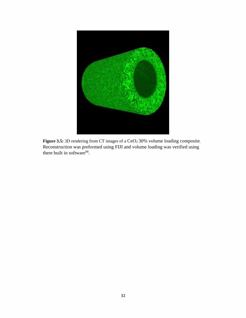
32
Figure 3.5: 3D rendering from CT images of a CeO2 30% volume loading composite.
Reconstruction was preformed using FIJI and volume loading was verified using
there built in software66.
33
CHAPTER 4: EXPERIMENTAL DIELECTRIC TESTING RESULTS
For the purpose of investigating the aims of this study, the theoretical output of the mixture
equations are compared to the experimentally measured composite values. In this chapter each
powder’s dielectric constant from literature are used to solve the individual mixture equations for
volume loadings of 1-50%. These results are mapped against a scatter plot of the experimental
values obtained using the coaxial airline method for volume loadings of 5%, 10%, 20%, and 30%.
The scatter plots are comprised of the 1601 data points taken from 1-10 GHz for each of the 24
individual composites, with 6 composites being tested at each volume loading. The scatter plots
show the averaged dielectric constant for each of the volume loading along with an associated t-
distribution error bar that shows their range of values corresponding to the unique volume loadings.
This is a necessary distribution because of the variability of the dipole-dipole interactions from
one measurement to the next55.
The absolute percent error for individual volume loadings are calculated to obtain a better
understanding of volume loadings effect on each mixture equations precision. The absolute percent
error is calculated based on the difference between the average dielectric constant of the mixture
and the output of the mixture equation at the corresponding volume loading. This numerical
analysis helps to validate what is seen graphically and to help isolate the study of each volume
loading. While the graphical results can be used mainly to study the trends of the equations as
volume loading increases and to a lesser extent the individual accuracy of each volume loading.
With specific focus paid to how the dielectric inclusion ratio (휀𝑝/휀𝑚) for powder to paraffin affects
equation accuracy, for both volume loadings and mixture equation.
4.1 Silicon Dioxide Composite Testing Results
The theoretical outcomes of the mixture equations as a function of volume loading are
graphed against the experimental scatter plot data in Figures 4.1-4.10 for SiO2. The mixture
equation uses the dielectric constant of SiO2 (휀𝑝 = 3.5) from literate and the measured dielectric
constant of paraffin (휀𝑚 = 2.3) to calculate the output. These compounds were found to have a
dielectric inclusion ration of 휀𝑝/휀𝑚 =1.5. The absolute percent error between the different
measured SiO2 composite and the theoretical output of each mixture equation are represented in
Tables 4.1-4.10.
4.1.1 Theoretical Parallel Mixing Equation Results for SiO2
The Parallel Mixing equation is the first equation looked at for SiO2, an analysis of its
accuracy across volume loadings can be obtained relatively easily. It had a calculated average
percent error across all volume loadings of 1.73% within never more than 3.04% error for any
single volume loading. It should be noted from Figure 4.1 that the equation varies outside of the t-
distribution at high volume loadings (>20%) Even though when the prediction does vary outside
of the t-distribution at high volume loadings the absolute error still remains less than 5%.
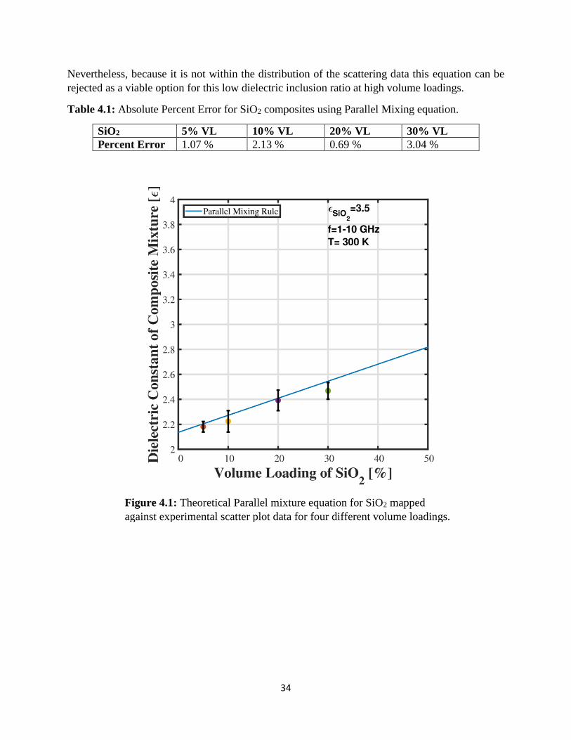
34
Nevertheless, because it is not within the distribution of the scattering data this equation can be
rejected as a viable option for this low dielectric inclusion ratio at high volume loadings.
Table 4.1: Absolute Percent Error for SiO2 composites using Parallel Mixing equation.
SiO2 5% VL 10% VL 20% VL 30% VL
Percent Error 1.07 % 2.13 % 0.69 % 3.04 %
Figure 4.1: Theoretical Parallel mixture equation for SiO2 mapped
against experimental scatter plot data for four different volume loadings.
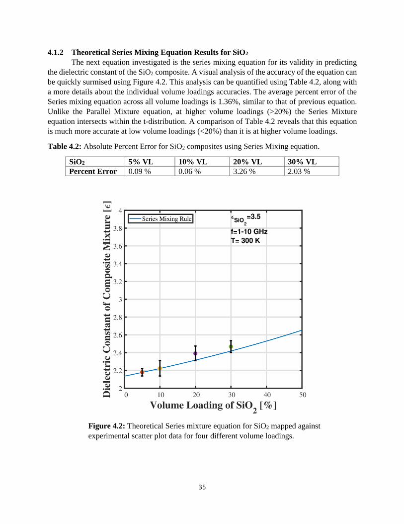
35
4.1.2 Theoretical Series Mixing Equation Results for SiO2
The next equation investigated is the series mixing equation for its validity in predicting
the dielectric constant of the SiO2 composite. A visual analysis of the accuracy of the equation can
be quickly surmised using Figure 4.2. This analysis can be quantified using Table 4.2, along with
a more details about the individual volume loadings accuracies. The average percent error of the
Series mixing equation across all volume loadings is 1.36%, similar to that of previous equation.
Unlike the Parallel Mixture equation, at higher volume loadings (>20%) the Series Mixture
equation intersects within the t-distribution. A comparison of Table 4.2 reveals that this equation
is much more accurate at low volume loadings (<20%) than it is at higher volume loadings.
Table 4.2: Absolute Percent Error for SiO2 composites using Series Mixing equation.
SiO2 5% VL 10% VL 20% VL 30% VL
Percent Error 0.09 % 0.06 % 3.26 % 2.03 %
Figure 4.2: Theoretical Series mixture equation for SiO2 mapped against
experimental scatter plot data for four different volume loadings.
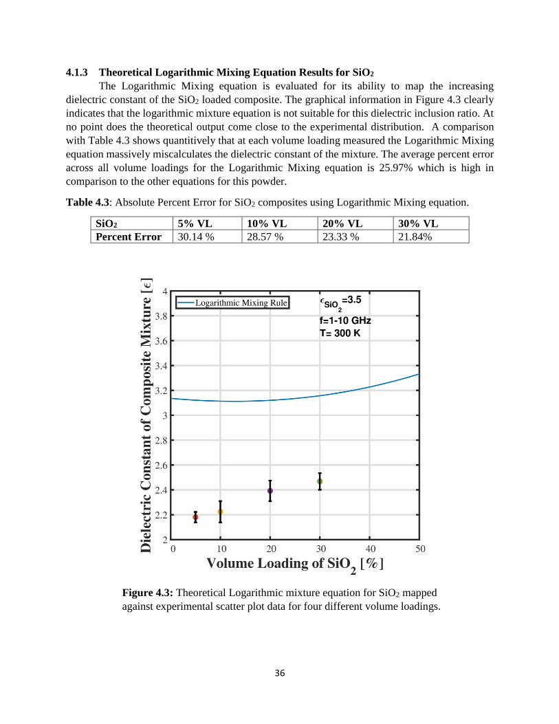
36
4.1.3 Theoretical Logarithmic Mixing Equation Results for SiO2
The Logarithmic Mixing equation is evaluated for its ability to map the increasing
dielectric constant of the SiO2 loaded composite. The graphical information in Figure 4.3 clearly
indicates that the logarithmic mixture equation is not suitable for this dielectric inclusion ratio. At
no point does the theoretical output come close to the experimental distribution. A comparison
with Table 4.3 shows quantitively that at each volume loading measured the Logarithmic Mixing
equation massively miscalculates the dielectric constant of the mixture. The average percent error
across all volume loadings for the Logarithmic Mixing equation is 25.97% which is high in
comparison to the other equations for this powder.
Table 4.3: Absolute Percent Error for SiO2 composites using Logarithmic Mixing equation.
SiO2 5% VL 10% VL 20% VL 30% VL
Percent Error 30.14 % 28.57 % 23.33 % 21.84%
Figure 4.3: Theoretical Logarithmic mixture equation for SiO2 mapped
against experimental scatter plot data for four different volume loadings.
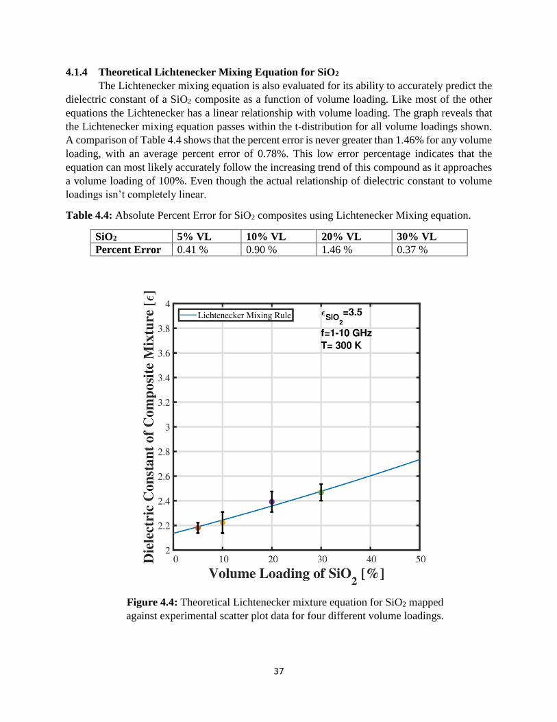
37
4.1.4 Theoretical Lichtenecker Mixing Equation for SiO2
The Lichtenecker mixing equation is also evaluated for its ability to accurately predict the
dielectric constant of a SiO2 composite as a function of volume loading. Like most of the other
equations the Lichtenecker has a linear relationship with volume loading. The graph reveals that
the Lichtenecker mixing equation passes within the t-distribution for all volume loadings shown.
A comparison of Table 4.4 shows that the percent error is never greater than 1.46% for any volume
loading, with an average percent error of 0.78%. This low error percentage indicates that the
equation can most likely accurately follow the increasing trend of this compound as it approaches
a volume loading of 100%. Even though the actual relationship of dielectric constant to volume
loadings isn’t completely linear.
Table 4.4: Absolute Percent Error for SiO2 composites using Lichtenecker Mixing equation.
SiO2 5% VL 10% VL 20% VL 30% VL
Percent Error 0.41 % 0.90 % 1.46 % 0.37 %
Figure 4.4: Theoretical Lichtenecker mixture equation for SiO2 mapped
against experimental scatter plot data for four different volume loadings.
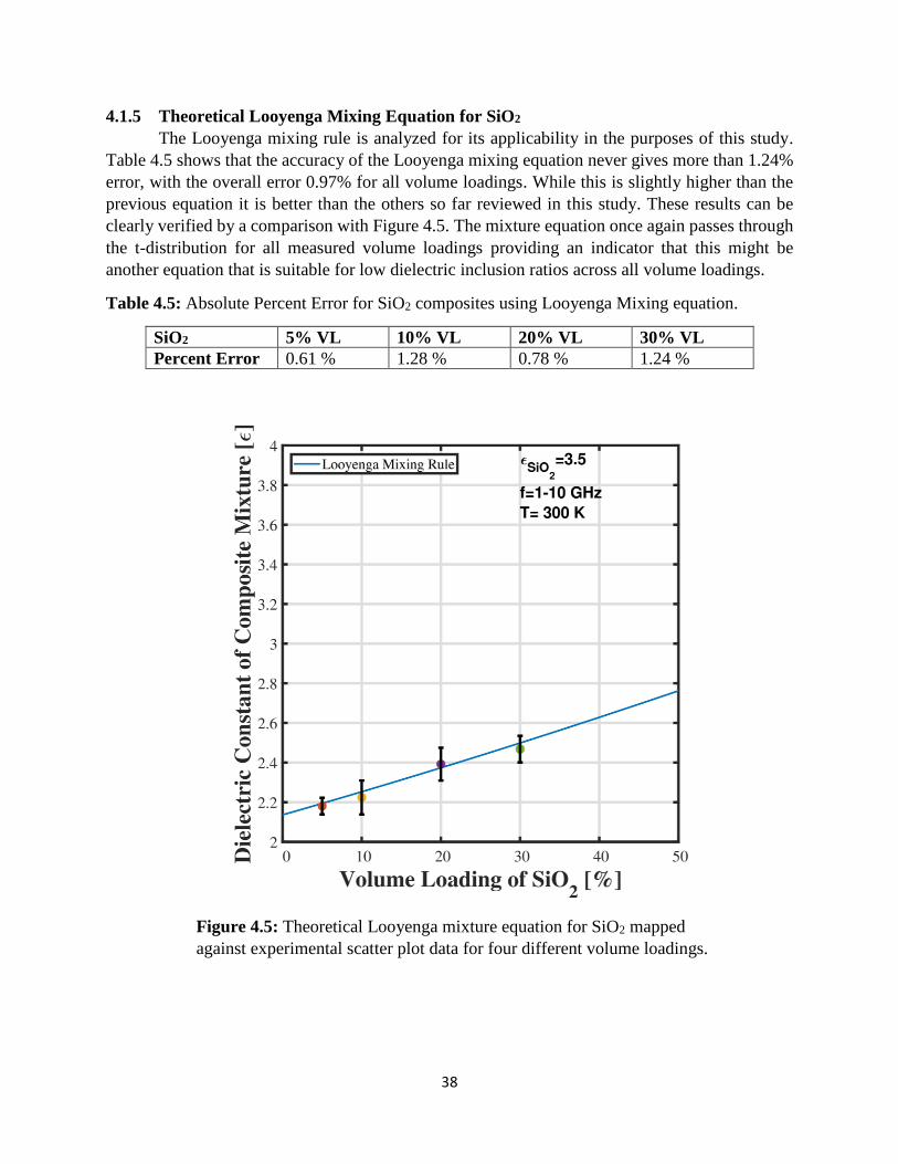
38
4.1.5 Theoretical Looyenga Mixing Equation for SiO2
The Looyenga mixing rule is analyzed for its applicability in the purposes of this study.
Table 4.5 shows that the accuracy of the Looyenga mixing equation never gives more than 1.24%
error, with the overall error 0.97% for all volume loadings. While this is slightly higher than the
previous equation it is better than the others so far reviewed in this study. These results can be
clearly verified by a comparison with Figure 4.5. The mixture equation once again passes through
the t-distribution for all measured volume loadings providing an indicator that this might be
another equation that is suitable for low dielectric inclusion ratios across all volume loadings.
Table 4.5: Absolute Percent Error for SiO2 composites using Looyenga Mixing equation.
SiO2 5% VL 10% VL 20% VL 30% VL
Percent Error 0.61 % 1.28 % 0.78 % 1.24 %
Figure 4.5: Theoretical Looyenga mixture equation for SiO2 mapped
against experimental scatter plot data for four different volume loadings.
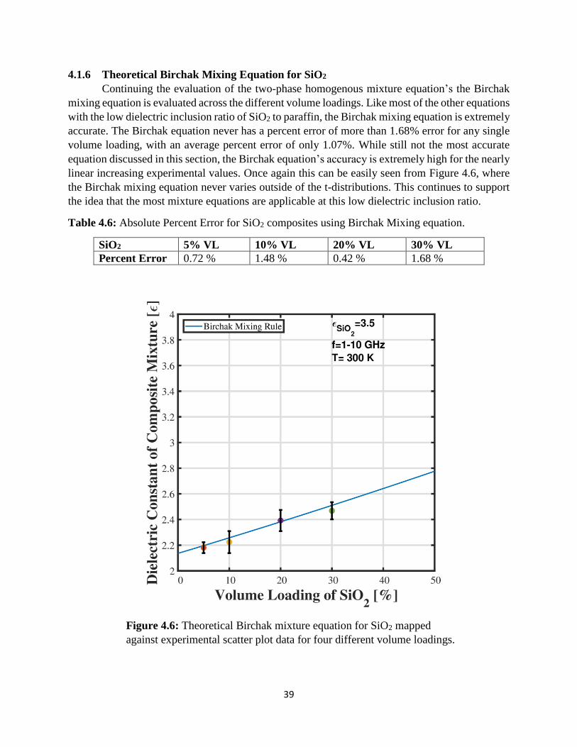
39
4.1.6 Theoretical Birchak Mixing Equation for SiO2
Continuing the evaluation of the two-phase homogenous mixture equation’s the Birchak
mixing equation is evaluated across the different volume loadings. Like most of the other equations
with the low dielectric inclusion ratio of SiO2 to paraffin, the Birchak mixing equation is extremely
accurate. The Birchak equation never has a percent error of more than 1.68% error for any single
volume loading, with an average percent error of only 1.07%. While still not the most accurate
equation discussed in this section, the Birchak equation’s accuracy is extremely high for the nearly
linear increasing experimental values. Once again this can be easily seen from Figure 4.6, where
the Birchak mixing equation never varies outside of the t-distributions. This continues to support
the idea that the most mixture equations are applicable at this low dielectric inclusion ratio.
Table 4.6: Absolute Percent Error for SiO2 composites using Birchak Mixing equation.
SiO2 5% VL 10% VL 20% VL 30% VL
Percent Error 0.72 % 1.48 % 0.42 % 1.68 %
Figure 4.6: Theoretical Birchak mixture equation for SiO2 mapped
against experimental scatter plot data for four different volume loadings.
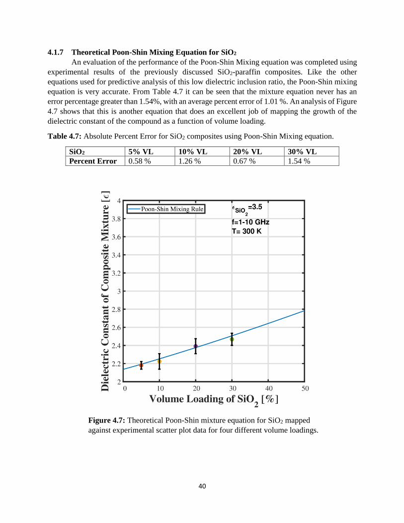
40
4.1.7 Theoretical Poon-Shin Mixing Equation for SiO2
An evaluation of the performance of the Poon-Shin Mixing equation was completed using
experimental results of the previously discussed SiO2-paraffin composites. Like the other
equations used for predictive analysis of this low dielectric inclusion ratio, the Poon-Shin mixing
equation is very accurate. From Table 4.7 it can be seen that the mixture equation never has an
error percentage greater than 1.54%, with an average percent error of 1.01 %. An analysis of Figure
4.7 shows that this is another equation that does an excellent job of mapping the growth of the
dielectric constant of the compound as a function of volume loading.
Table 4.7: Absolute Percent Error for SiO2 composites using Poon-Shin Mixing equation.
SiO2 5% VL 10% VL 20% VL 30% VL
Percent Error 0.58 % 1.26 % 0.67 % 1.54 %
Figure 4.7: Theoretical Poon-Shin mixture equation for SiO2 mapped
against experimental scatter plot data for four different volume loadings.

41
4.1.8 Theoretical Effective Medium Theory Mixing Equation for SiO2
The EMT mixing equation is assessed for its capability to correctly predict the dielectric
constant of SiO2 composites. Unlike most of the other equations the EMT has a slightly parabolic
relationship with volume loading, this is a factor of the added shape factor variable in the EMT
equation. The graph in Figure 4.8, reveals that the EMT mixing equation passes within the t-
distribution for all volume loadings shown despite this more parabolic shape. A comparison of
Table 4.4 shows that the percent error is never greater than 1.76% for any volume loading, with
an average percent error of 0.94%. This low error percentage indicates that the equation can
accurately follow the increasing trend of this compound as it approaches the pure powder value.
Table 4.8: Absolute Percent Error for SiO2 composites using EMT Mixing equation.
SiO2 5% VL 10% VL 20% VL 30% VL
Percent Error 0.98 % 1.76 % 0.65 % 0.36 %
Figure 4.8: Theoretical EMT mixture equation for SiO2 mapped
against experimental scatter plot data for four different volume
loadings.
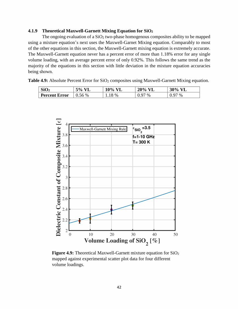
42
4.1.9 Theoretical Maxwell-Garnett Mixing Equation for SiO2
The ongoing evaluation of a SiO2 two-phase homogenous composites ability to be mapped
using a mixture equation’s next uses the Maxwell-Garnet Mixing equation. Comparably to most
of the other equations in this section, the Maxwell-Garnett mixing equation is extremely accurate.
The Maxwell-Garnett equation never has a percent error of more than 1.18% error for any single
volume loading, with an average percent error of only 0.92%. This follows the same trend as the
majority of the equations in this section with little deviation in the mixture equation accuracies
being shown.
Table 4.9: Absolute Percent Error for SiO2 composites using Maxwell-Garnett Mixing equation.
SiO2 5% VL 10% VL 20% VL 30% VL
Percent Error 0.56 % 1.18 % 0.97 % 0.97 %
Figure 4.9: Theoretical Maxwell-Garnett mixture equation for SiO2
mapped against experimental scatter plot data for four different
volume loadings.

43
4.1.10 Theoretical Jayasundere-Smith Mixing Equation for SiO2
The final equation examined was the Jayasundere-Smith mixing equation, Table 4.10
shows that the accuracy of the Looyenga mixing equation never becomes more than 2.6% error.
With the overall error 1.18% for all volume loadings, these results can be clearly clarified by a
comparison with Figure 4.10. The mixture equation once again passes through the t-distribution
for all measured volume loadings providing an indicator that this might be another equation that
is suitable for low dielectric inclusion ratios. However, at high volume loadings (>30%) the
equation is barely inside the t-distribution, indicating that this equation might not be suitable for
high volume loadings.
Table 4.10: Absolute Percent Error for SiO2 composites using Jayasundere-Smith Mixing
equation.
SiO2 5% VL 10% VL 20% VL 30% VL
Percent Error 0.62 % 1.42 % 0.12 % 2.54 %
Figure 4.10: Theoretical Jayasundere-Smith mixture equation for
SiO2 mapped against experimental scatter plot data for four different
volume loadings.
44
4.2 Aluminum Oxide Dioxide Composite Testing Results
After evaluating all the mixture equations for the low dielectric inclusion ration of 1.5 for
SiO2 to paraffin the study next looks at a Al2O3 as the inclusion powder. The higher dielectric
constant of Al2O3 (휀𝑝 = 9.8) results in a dielectric inclusion ratio of 휀𝑝/휀𝑚 =4.3. The theoretical
outcomes of the mixture equations as a function of volume loading are graphed against the
experimental scatter plot data in Figures 4.11-4.20 for Al2O3. The absolute percent error between
the different measured Al2O3composite and the theoretical output of each mixture equation are
represented in Tables 4.11-4.20.
4.2.1 Theoretical Parallel Mixing Equation Results for Al2O3
The results of the of the Parallel Mixing equation’s ability to predict Al2O3 compounds
dielectric constant are discussed in this section. The Parallel Mixing equation was found to have
an average percent error across all volume loadings of 14.82% this is an increase from the previous
constitutive powder by 13.09%. Figure 4.11 and Table 4.11 shows that the parallel mixing rule
does a terrible job of predicting the behavior of the composites dielectric constant as volume
loading increases. It can be seen from the Figure that the behavior of the measured composite’s
dielectric constant no longer behaves linearly. This is a direct consequence of the dielectric
inclusion ratio. The increase in inclusion ratio corresponds to the large increase in error seen from
the previous section.
Table 4.11: Absolute Percent Error for Al2O3 composites using the Parallel Mixing equation.
Al2O3 5% VL 10% VL 20% VL 30% VL
Percent Error 4.78 % 7.37 % 19.44 % 27.68 %
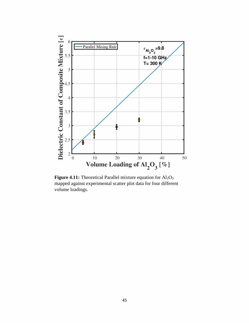
45
Figure 4.11: Theoretical Parallel mixture equation for Al2O3
mapped against experimental scatter plot data for four different
volume loadings.
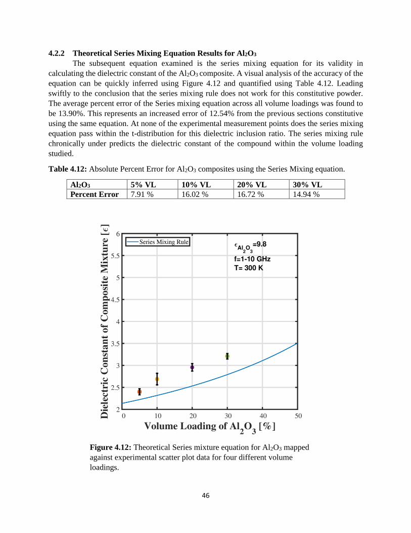
46
4.2.2 Theoretical Series Mixing Equation Results for Al2O3
The subsequent equation examined is the series mixing equation for its validity in
calculating the dielectric constant of the Al2O3 composite. A visual analysis of the accuracy of the
equation can be quickly inferred using Figure 4.12 and quantified using Table 4.12. Leading
swiftly to the conclusion that the series mixing rule does not work for this constitutive powder.
The average percent error of the Series mixing equation across all volume loadings was found to
be 13.90%. This represents an increased error of 12.54% from the previous sections constitutive
using the same equation. At none of the experimental measurement points does the series mixing
equation pass within the t-distribution for this dielectric inclusion ratio. The series mixing rule
chronically under predicts the dielectric constant of the compound within the volume loading
studied.
Table 4.12: Absolute Percent Error for Al2O3 composites using the Series Mixing equation.
Al2O3 5% VL 10% VL 20% VL 30% VL
Percent Error 7.91 % 16.02 % 16.72 % 14.94 %
Figure 4.12: Theoretical Series mixture equation for Al2O3 mapped
against experimental scatter plot data for four different volume
loadings.
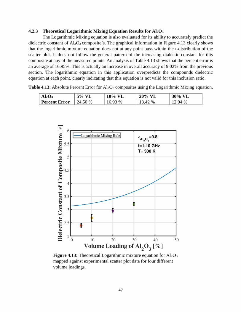
47
4.2.3 Theoretical Logarithmic Mixing Equation Results for Al2O3
The Logarithmic Mixing equation is also evaluated for its ability to accurately predict the
dielectric constant of Al2O3 composite’s. The graphical information in Figure 4.13 clearly shows
that the logarithmic mixture equation does not at any point pass within the t-distribution of the
scatter plot. It does not follow the general pattern of the increasing dialectic constant for this
composite at any of the measured points. An analysis of Table 4.13 shows that the percent error is
an average of 16.95%. This is actually an increase in overall accuracy of 9.02% from the previous
section. The logarithmic equation in this application overpredicts the compounds dielectric
equation at each point, clearly indicating that this equation is not valid for this inclusion ratio.
Table 4.13: Absolute Percent Error for Al2O3 composites using the Logarithmic Mixing equation.
Al2O3 5% VL 10% VL 20% VL 30% VL
Percent Error 24.50 % 16.93 % 13.42 % 12.94 %
Figure 4.13: Theoretical Logarithmic mixture equation for Al2O3
mapped against experimental scatter plot data for four different
volume loadings.

48
4.2.4 Theoretical Lichtenecker Mixing Equation for Al2O3
Continuing the evaluation of Al2O3 two-phase homogenous composites, the Lichtenecker
mixing equation is assessed. Like most of the other equations in this section, the Lichtenecker
mixing equation struggles to map the behavior of the changes in dielectric constant as a function
of volume loading. It is still relatively accurate despite predicting a higher dielectric constant rate
of change then what is seen experimentally. The Lichtenecker equation has an average percent
error of 4.77% an increase of only 3.99%. Figure 4.14 shows that despite this good accuracy
(<5%) the Lichtenecker mixing equation only passes through the t-distribution at the 20% volume
loading. This continues to support the idea that increasing the dielectric inclusion ratio leads to
more difficulty in predicting the behavior of the composite.
Table 4.14: Absolute Percent Error for Al2O3 composites using the Lichtenecker Mixing equation.
Al2O3 5% VL 10% VL 20% VL 30% VL
Percent Error 4.07 % 8.08 % 2.02 % 4.92 %
Figure 4.14: Theoretical Lichtenecker mixture equation for Al2O3
mapped against experimental scatter plot data for four different
volume loadings.
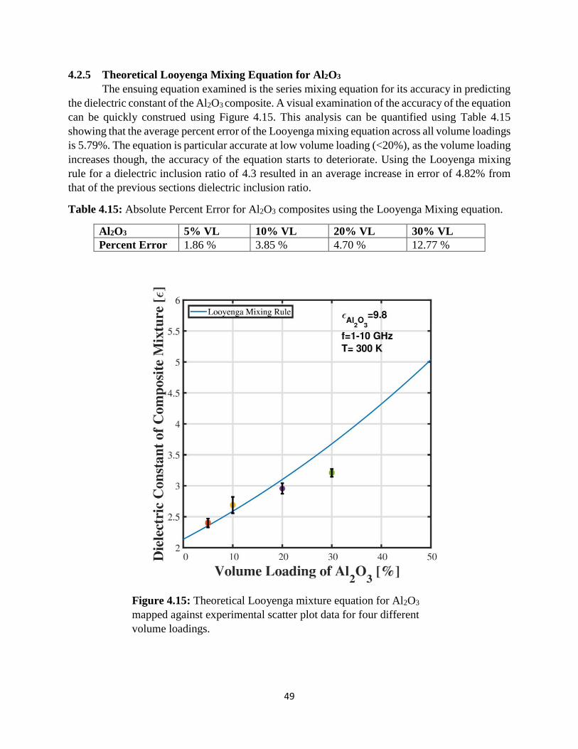
49
4.2.5 Theoretical Looyenga Mixing Equation for Al2O3
The ensuing equation examined is the series mixing equation for its accuracy in predicting
the dielectric constant of the Al2O3 composite. A visual examination of the accuracy of the equation
can be quickly construed using Figure 4.15. This analysis can be quantified using Table 4.15
showing that the average percent error of the Looyenga mixing equation across all volume loadings
is 5.79%. The equation is particular accurate at low volume loading (<20%), as the volume loading
increases though, the accuracy of the equation starts to deteriorate. Using the Looyenga mixing
rule for a dielectric inclusion ratio of 4.3 resulted in an average increase in error of 4.82% from
that of the previous sections dielectric inclusion ratio.
Table 4.15: Absolute Percent Error for Al2O3 composites using the Looyenga Mixing equation.
Al2O3 5% VL 10% VL 20% VL 30% VL
Percent Error 1.86 % 3.85 % 4.70 % 12.77 %
Figure 4.15: Theoretical Looyenga mixture equation for Al2O3
mapped against experimental scatter plot data for four different
volume loadings.
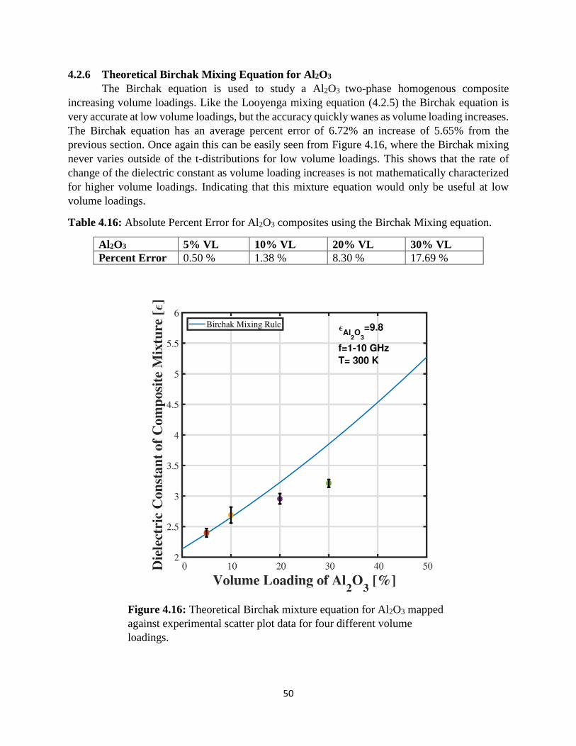
50
4.2.6 Theoretical Birchak Mixing Equation for Al2O3
The Birchak equation is used to study a Al2O3 two-phase homogenous composite
increasing volume loadings. Like the Looyenga mixing equation (4.2.5) the Birchak equation is
very accurate at low volume loadings, but the accuracy quickly wanes as volume loading increases.
The Birchak equation has an average percent error of 6.72% an increase of 5.65% from the
previous section. Once again this can be easily seen from Figure 4.16, where the Birchak mixing
never varies outside of the t-distributions for low volume loadings. This shows that the rate of
change of the dielectric constant as volume loading increases is not mathematically characterized
for higher volume loadings. Indicating that this mixture equation would only be useful at low
volume loadings.
Table 4.16: Absolute Percent Error for Al2O3 composites using the Birchak Mixing equation.
Al2O3 5% VL 10% VL 20% VL 30% VL
Percent Error 0.50 % 1.38 % 8.30 % 17.69 %
Figure 4.16: Theoretical Birchak mixture equation for Al2O3 mapped
against experimental scatter plot data for four different volume
loadings.

51
4.2.7 Theoretical Poon-Shin Mixing Equation for Al2O3
Using the Poon-Shin Mixing equation experimental results of the previously discussed
Al2O3-paraffin composites are studied. Like the other equations used for predictive analysis of this
dielectric inclusion ratio, the Poon-Shin mixing equation is not extremely accurate. From Table
4.7 it can be seen that the mixture equation’s accuracy is good at 5 and 20 percent but poor at 10
and 30 percent, with an average percent error of 5.50 %, which is an increase of 4.49% from the
same analysis with SiO2. An analysis of Figure 4.17 shows that this is another equation that does
a decent job of mapping the growth of the dielectric constant. While some of the other equation
discussed in this study are only good at lower volume loadings, the Poon-Shin equation
comparatively predicts slightly lesser values for the dielectric constant at low volume loading and
slightly greater values at higher volume loadings.
Table 4.17: Absolute Percent Error for Al2O3 composites using the Poon-Shin Mixing equation.
Al2O3 5% VL 10% VL 20% VL 30% VL
Percent Error 3.39 % 6.46 % 1.62 % 10.54 %
Figure 4.17: Theoretical Poon-Shin mixture equation for Al2O3
mapped against experimental scatter plot data for four different
volume loadings.

52
4.2.8 Theoretical Effective Medium Theory Mixing Equation for Al2O3
The EMT mixing equation is evaluated for its ability to accurately predict the dielectric
constant of a Al2O3 composite as a function of volume loading. Unlike the other equations the
EMT’s shape factor variable allows it to take unique mathematical rates of change, with slower
rates of change being expressed at higher volume loadings. The graph in Figure 4.18, reveals that
the EMT mixing equation passes within the t-distribution for all volume loadings shown. This is a
significant change from the other equations shown in this section. A comparison of Table 4.14
shows that the percent error stays consistently low for all volume loading, with an average percent
error of 1.16%. This low error percentage indicates that the equation can accurately follow the
increasing trend of this compound within the parameters studied.
Table 4.18: Absolute Percent Error for Al2O3 composites using the EMT Mixing equation.
Al2O3 5% VL 10% VL 20% VL 30% VL
Percent Error 2.43 % 0.16 % 1.82 % 0.24 %
Figure 4.18: Theoretical EMT mixture equation for Al2O 3 mapped
against experimental scatter plot data for four different volume
loadings.
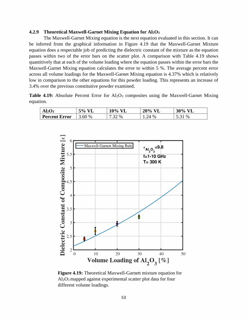
53
4.2.9 Theoretical Maxwell-Garnet Mixing Equation for Al2O3
The Maxwell-Garnet Mixing equation is the next equation evaluated in this section. It can
be inferred from the graphical information in Figure 4.19 that the Maxwell-Garnet Mixture
equation does a respectable job of predicting the dielectric constant of the mixture as the equation
passes within two of the error bars on the scatter plot. A comparison with Table 4.19 shows
quantitively that at each of the volume loading where the equation passes within the error bars the
Maxwell-Garnet Mixing equation calculates the error to within 5 %. The average percent error
across all volume loadings for the Maxwell-Garnet Mixing equation is 4.37% which is relatively
low in comparison to the other equations for this powder loading. This represents an increase of
3.4% over the previous constitutive powder examined.
Table 4.19: Absolute Percent Error for Al2O3 composites using the Maxwell-Garnet Mixing
equation.
Al2O3 5% VL 10% VL 20% VL 30% VL
Percent Error 3.60 % 7.32 % 1.24 % 5.31 %
Figure 4.19: Theoretical Maxwell-Garnett mixture equation for
Al2O3 mapped against experimental scatter plot data for four
different volume loadings.
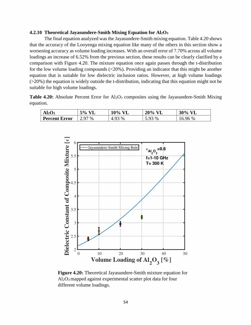
54
4.2.10 Theoretical Jayasundere-Smith Mixing Equation for Al2O3
The final equation analyzed was the Jayasundere-Smith mixing equation. Table 4.20 shows
that the accuracy of the Looyenga mixing equation like many of the others in this section show a
worsening accuracy as volume loading increases. With an overall error of 7.70% across all volume
loadings an increase of 6.52% from the previous section, these results can be clearly clarified by a
comparison with Figure 4.20. The mixture equation once again passes through the t-distribution
for the low volume loading compounds (<20%). Providing an indicator that this might be another
equation that is suitable for low dielectric inclusion ratios. However, at high volume loadings
(>20%) the equation is widely outside the t-distribution, indicating that this equation might not be
suitable for high volume loadings.
Table 4.20: Absolute Percent Error for Al2O3 composites using the Jayasundere-Smith Mixing
equation.
Al2O3 5% VL 10% VL 20% VL 30% VL
Percent Error 2.97 % 4.93 % 5.93 % 16.96 %
Figure 4.20: Theoretical Jayasundere-Smith mixture equation for
Al2O3 mapped against experimental scatter plot data for four
different volume loadings.
55
4.3 Cerium Dioxide Composite Testing Results
The study next looked at a CeO2 as the inclusion powder to ascertain the accuracy of the
mixture equations for this work. The higher dielectric constant of CeO2 (휀𝑝 = 21.3) results in a
dielectric inclusion ratio of 휀𝑝/휀𝑚 =10. The theoretical outcomes of the mixture equations as a
function of volume loading are graphed against the experimental scatter plot data in Figures 4.21-
4.30 for CeO2. The absolute percent error between the different measured CeO2 composite and the
theoretical output of each mixture equation are represented in Tables 4.21-4.30.
4.3.1 Theoretical Parallel Mixing Equation Results for CeO2
Like the previous section the first equation evaluated in the Parallel Mixing equation. The
Parallel Mixing equation has an average percent error across all volume loadings of 27.99%. This
is an increase of 13.77% error from the same equation using Al2O3 as the constitutive material.
Figure 4.21 and Table 4.21 shows that the parallel mixing rule does a terrible job of predicting the
behavior of the composites dielectric constant as volume loading increases just like for the
previously studied powder. It can be seen from the Figure that the behavior of the measured
composite’s dielectric constant behaves exponentially whilst the parallel mixture equation only
predicts a linear growth. The effects of the increased dielectric inclusion ratio on the accuracy of
the mixture equations can clearly be seen in this section.
Table 4.21: Absolute Percent Error for CeO2 composites using the Parallel Mixing equation.
CeO2 5% VL 10% VL 20% VL 30% VL
Percent Error 17.71 % 27.70 % 33.01 % 33.54 %
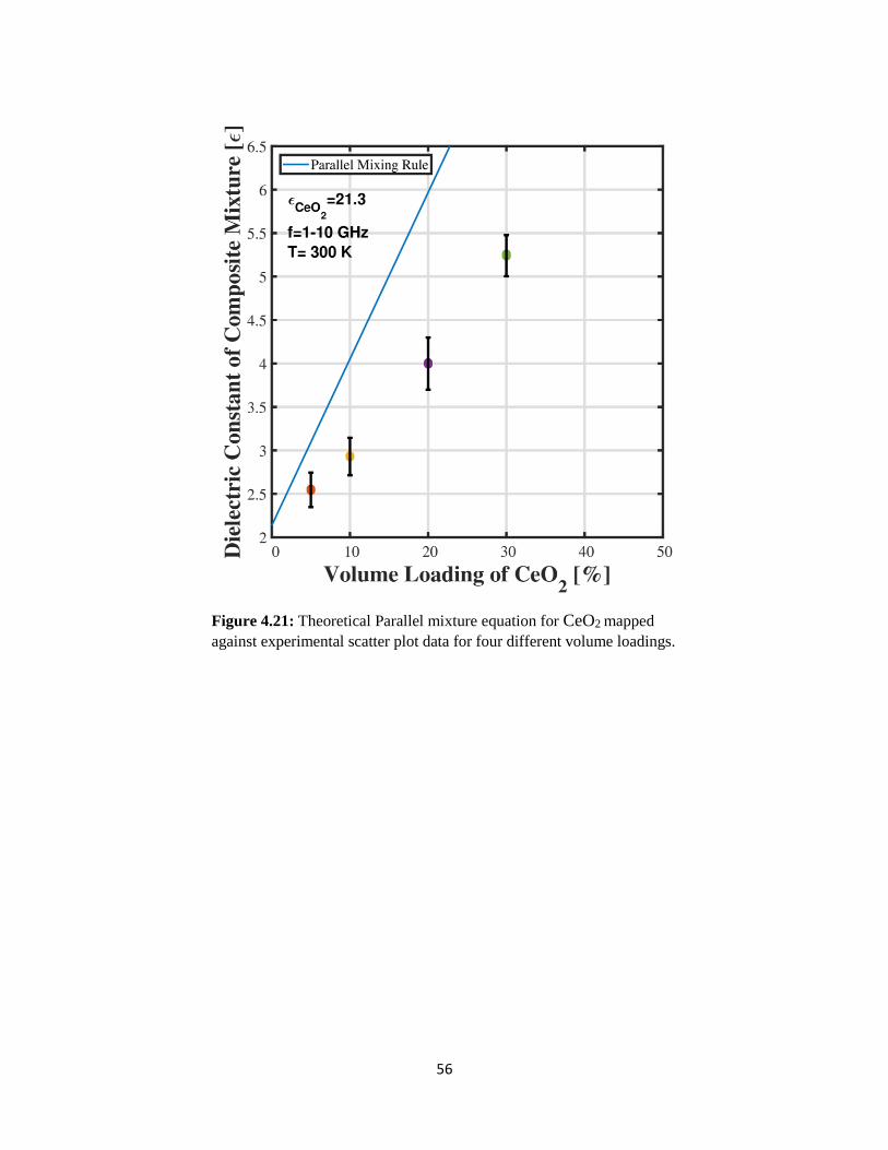
56
Figure 4.21: Theoretical Parallel mixture equation for CeO2 mapped
against experimental scatter plot data for four different volume loadings.
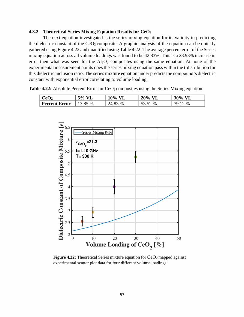
57
4.3.2 Theoretical Series Mixing Equation Results for CeO2
The next equation investigated is the series mixing equation for its validity in predicting
the dielectric constant of the CeO2 composite. A graphic analysis of the equation can be quickly
gathered using Figure 4.22 and quantified using Table 4.22. The average percent error of the Series
mixing equation across all volume loadings was found to be 42.83%. This is a 28.93% increase in
error then what was seen for the Al2O3 composites using the same equation. At none of the
experimental measurement points does the series mixing equation pass within the t-distribution for
this dielectric inclusion ratio. The series mixture equation under predicts the compound’s dielectric
constant with exponential error correlating to volume loading.
Table 4.22: Absolute Percent Error for CeO2 composites using the Series Mixing equation.
CeO2 5% VL 10% VL 20% VL 30% VL
Percent Error 13.85 % 24.83 % 53.52 % 79.12 %
Figure 4.22: Theoretical Series mixture equation for CeO2 mapped against
experimental scatter plot data for four different volume loadings.
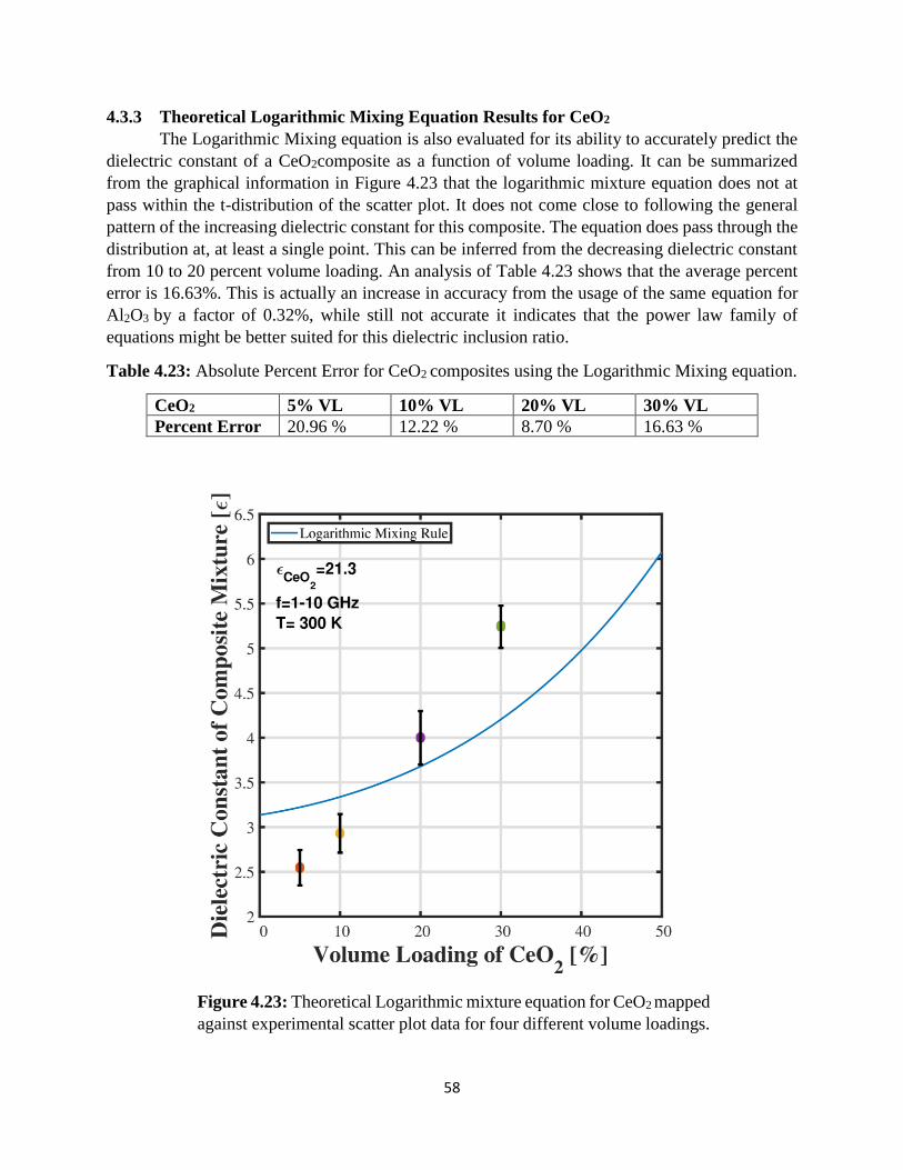
58
4.3.3 Theoretical Logarithmic Mixing Equation Results for CeO2
The Logarithmic Mixing equation is also evaluated for its ability to accurately predict the
dielectric constant of a CeO2composite as a function of volume loading. It can be summarized
from the graphical information in Figure 4.23 that the logarithmic mixture equation does not at
pass within the t-distribution of the scatter plot. It does not come close to following the general
pattern of the increasing dielectric constant for this composite. The equation does pass through the
distribution at, at least a single point. This can be inferred from the decreasing dielectric constant
from 10 to 20 percent volume loading. An analysis of Table 4.23 shows that the average percent
error is 16.63%. This is actually an increase in accuracy from the usage of the same equation for
Al2O3 by a factor of 0.32%, while still not accurate it indicates that the power law family of
equations might be better suited for this dielectric inclusion ratio.
Table 4.23: Absolute Percent Error for CeO2 composites using the Logarithmic Mixing equation.
CeO2 5% VL 10% VL 20% VL 30% VL
Percent Error 20.96 % 12.22 % 8.70 % 16.63 %
Figure 4.23: Theoretical Logarithmic mixture equation for CeO2 mapped
against experimental scatter plot data for four different volume loadings.
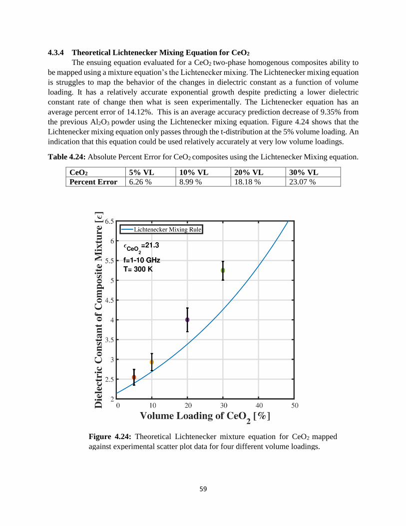
59
4.3.4 Theoretical Lichtenecker Mixing Equation for CeO2
The ensuing equation evaluated for a CeO2 two-phase homogenous composites ability to
be mapped using a mixture equation’s the Lichtenecker mixing. The Lichtenecker mixing equation
is struggles to map the behavior of the changes in dielectric constant as a function of volume
loading. It has a relatively accurate exponential growth despite predicting a lower dielectric
constant rate of change then what is seen experimentally. The Lichtenecker equation has an
average percent error of 14.12%. This is an average accuracy prediction decrease of 9.35% from
the previous Al2O3 powder using the Lichtenecker mixing equation. Figure 4.24 shows that the
Lichtenecker mixing equation only passes through the t-distribution at the 5% volume loading. An
indication that this equation could be used relatively accurately at very low volume loadings.
Table 4.24: Absolute Percent Error for CeO2 composites using the Lichtenecker Mixing equation.
CeO2 5% VL 10% VL 20% VL 30% VL
Percent Error 6.26 % 8.99 % 18.18 % 23.07 %
Figure 4.24: Theoretical Lichtenecker mixture equation for CeO2 mapped
against experimental scatter plot data for four different volume loadings.

60
4.3.5 Theoretical Looyenga Mixing Equation for CeO2
The Looyenga rule is next evaluated and compared to the previous sections results. A
graphical examination of the mixing equation can be quickly construed via Figure 4.25. The
average percent error of the Looyenga mixing equation across all volume loadings was found to
be 0.76%. This represents an extremely accurate equation for this application with the theoretical
output almost exactly predicting the compound’s experimental measurements. This analysis can
be quantified using Table 4.25. The usage of the Looyenga mixing rule in predicting the output of
the CeO2 compound represents an increase of 5.03 from the previous section. The Looyenga
mixing rule is able to exactly match the correlation between volume loading and dielectric
constant.
Table 4.25: Absolute Percent Error for CeO2 composites using the Looyenga Mixing equation.
CeO2 5% VL 10% VL 20% VL 30% VL
Percent Error 0.77 % 1.11 % 0.48 % 0.67 %
Figure 4.25: Theoretical Looyenga mixture equation for CeO2 mapped
against experimental scatter plot data for four different volume loadings.
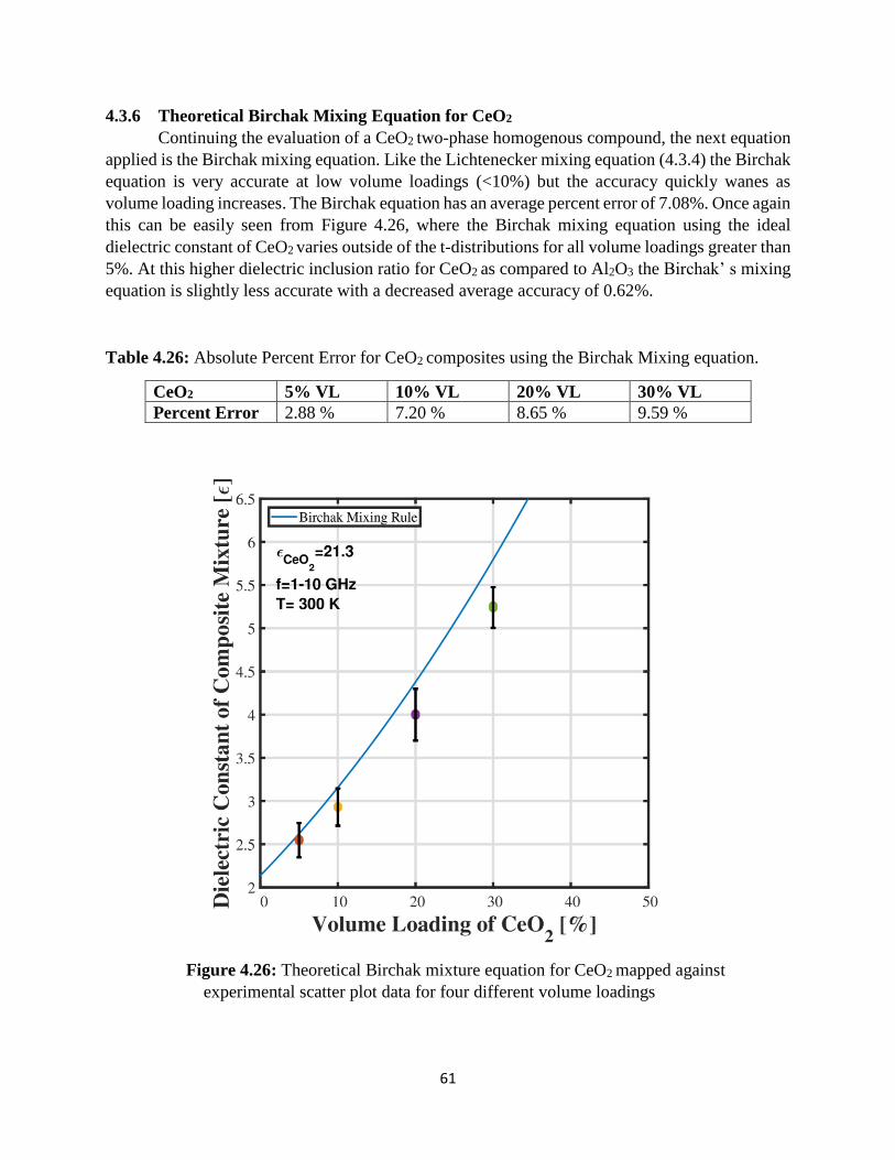
61
4.3.6 Theoretical Birchak Mixing Equation for CeO2
Continuing the evaluation of a CeO2 two-phase homogenous compound, the next equation
applied is the Birchak mixing equation. Like the Lichtenecker mixing equation (4.3.4) the Birchak
equation is very accurate at low volume loadings (<10%) but the accuracy quickly wanes as
volume loading increases. The Birchak equation has an average percent error of 7.08%. Once again
this can be easily seen from Figure 4.26, where the Birchak mixing equation using the ideal
dielectric constant of CeO2 varies outside of the t-distributions for all volume loadings greater than
5%. At this higher dielectric inclusion ratio for CeO2 as compared to Al2O3 the Birchak’ s mixing
equation is slightly less accurate with a decreased average accuracy of 0.62%.
Table 4.26: Absolute Percent Error for CeO2 composites using the Birchak Mixing equation.
CeO2 5% VL 10% VL 20% VL 30% VL
Percent Error 2.88 % 7.20 % 8.65 % 9.59 %
Figure 4.26: Theoretical Birchak mixture equation for CeO2 mapped against
experimental scatter plot data for four different volume loadings
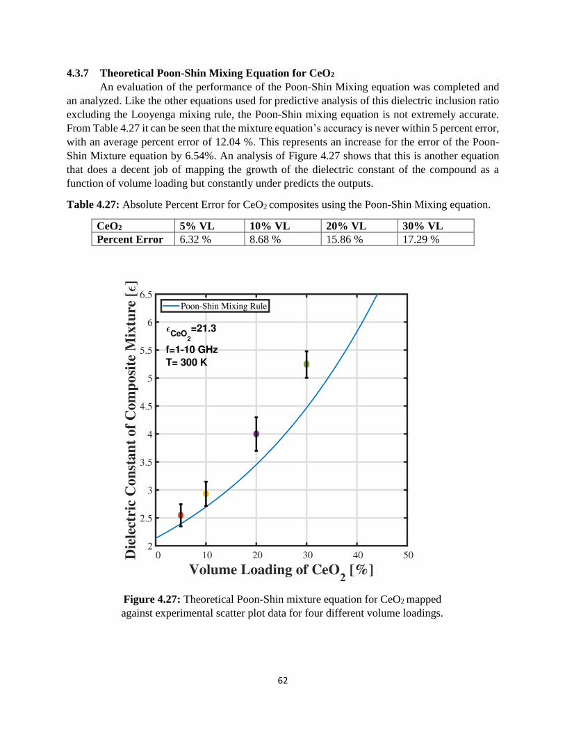
62
4.3.7 Theoretical Poon-Shin Mixing Equation for CeO2
An evaluation of the performance of the Poon-Shin Mixing equation was completed and
an analyzed. Like the other equations used for predictive analysis of this dielectric inclusion ratio
excluding the Looyenga mixing rule, the Poon-Shin mixing equation is not extremely accurate.
From Table 4.27 it can be seen that the mixture equation’s accuracy is never within 5 percent error,
with an average percent error of 12.04 %. This represents an increase for the error of the Poon-
Shin Mixture equation by 6.54%. An analysis of Figure 4.27 shows that this is another equation
that does a decent job of mapping the growth of the dielectric constant of the compound as a
function of volume loading but constantly under predicts the outputs.
Table 4.27: Absolute Percent Error for CeO2 composites using the Poon-Shin Mixing equation.
CeO2 5% VL 10% VL 20% VL 30% VL
Percent Error 6.32 % 8.68 % 15.86 % 17.29 %
Figure 4.27: Theoretical Poon-Shin mixture equation for CeO2 mapped
against experimental scatter plot data for four different volume loadings.
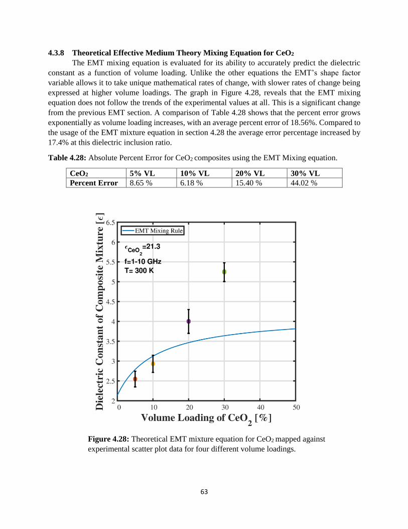
63
4.3.8 Theoretical Effective Medium Theory Mixing Equation for CeO2
The EMT mixing equation is evaluated for its ability to accurately predict the dielectric
constant as a function of volume loading. Unlike the other equations the EMT’s shape factor
variable allows it to take unique mathematical rates of change, with slower rates of change being
expressed at higher volume loadings. The graph in Figure 4.28, reveals that the EMT mixing
equation does not follow the trends of the experimental values at all. This is a significant change
from the previous EMT section. A comparison of Table 4.28 shows that the percent error grows
exponentially as volume loading increases, with an average percent error of 18.56%. Compared to
the usage of the EMT mixture equation in section 4.28 the average error percentage increased by
17.4% at this dielectric inclusion ratio.
Table 4.28: Absolute Percent Error for CeO2 composites using the EMT Mixing equation.
CeO2 5% VL 10% VL 20% VL 30% VL
Percent Error 8.65 % 6.18 % 15.40 % 44.02 %
Figure 4.28: Theoretical EMT mixture equation for CeO2 mapped against
experimental scatter plot data for four different volume loadings.
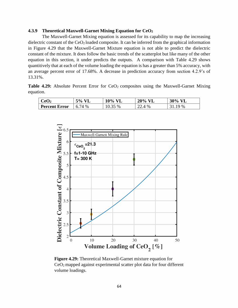
64
4.3.9 Theoretical Maxwell-Garnet Mixing Equation for CeO2
The Maxwell-Garnet Mixing equation is assessed for its capability to map the increasing
dielectric constant of the CeO2 loaded composite. It can be inferred from the graphical information
in Figure 4.29 that the Maxwell-Garnet Mixture equation is not able to predict the dielectric
constant of the mixture. It does follow the basic trends of the scatterplot but like many of the other
equation in this section, it under predicts the outputs. A comparison with Table 4.29 shows
quantitively that at each of the volume loading the equation is has a greater than 5% accuracy, with
an average percent error of 17.68%. A decrease in prediction accuracy from section 4.2.9’s of
13.31%.
Table 4.29: Absolute Percent Error for CeO2 composites using the Maxwell-Garnet Mixing
equation.
CeO2 5% VL 10% VL 20% VL 30% VL
Percent Error 6.74 % 10.35 % 22.4 % 31.19 %
Figure 4.29: Theoretical Maxwell-Garnet mixture equation for
CeO2 mapped against experimental scatter plot data for four different
volume loadings.
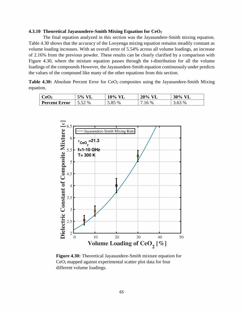
65
4.3.10 Theoretical Jayasundere-Smith Mixing Equation for CeO2
The final equation analyzed in this section was the Jayasundere-Smith mixing equation.
Table 4.30 shows that the accuracy of the Looyenga mixing equation remains steadily constant as
volume loading increases. With an overall error of 5.54% across all volume loadings, an increase
of 2.16% from the previous powder. These results can be clearly clarified by a comparison with
Figure 4.30, where the mixture equation passes through the t-distribution for all the volume
loadings of the compounds However, the Jayasundere-Smith equation continuously under predicts
the values of the compound like many of the other equations from this section.
Table 4.30: Absolute Percent Error for CeO2 composites using the Jayasundere-Smith Mixing
equation.
CeO2 5% VL 10% VL 20% VL 30% VL
Percent Error 5.52 % 5.85 % 7.16 % 3.63 %
Figure 4.30: Theoretical Jayasundere-Smith mixture equation for
CeO2 mapped against experimental scatter plot data for four
different volume loadings.
66
4.4 Titanium Dioxide Composite Testing Results
The last constitutive powder the study looked at was TiO2 for the purpose of ascertaining
the accuracy of the mixture equations for this work. The higher dielectric constant of TiO2 (휀𝑝 =
70) results in a dielectric inclusion ratio of 휀𝑝/휀𝑚 =30. The theoretical outcomes of the mixture
equations as a function of volume loading are graphed against the experimental scatter plot data in
Figures 4.31-4.40 for CeO2. The absolute percent error between the different measured CeO2
composite and the theoretical output of each mixture equation are represented in Tables 4.31-4.40.
4.4.1 Theoretical Parallel Mixing Equation Results for TiO2
The study once again takes a look at the Parallel Mixing equation to ascertain its accuracy
at this new dielectric inclusion ratio. The Parallel Mixing equation was found to have an average
percent error across all volume loadings of 56.78%. This is an increase of 28.79% error from the
same equation using CeO2 as the filler material, a direct consequence of the increased dielectric
inclusion ratio. Figure 4.31 and Table 4.31 shows that the parallel mixing rule does a terrible job
of predicting the behavior of the composites dielectric constant as volume loading increases. It can
be seen from the Figure that the behavior of the measured composite’s dielectric constant behaves
exponentially whilst the parallel mixture equation only predicts a linear growth.
Table 4.31: Absolute Percent Error for TiO2 composites using the Parallel Mixing equation.
CeO2 5% VL 10% VL 20% VL 30% VL
Percent Error 51.09 % 61.06 % 60.38 % 54.58 %

67
Figure 4.31: Theoretical Parallel mixture equation for TiO2
mapped against experimental scatter plot data for four different
volume loadings.

68
4.4.2 Theoretical Series Mixing Equation Results for TiO2
The next equation investigated is the series mixing equation for its validity in predicting
the dielectric constant of the TiO2 composite. A visual scrutiny of the precision of the equation can
be quickly surmised using Figure 4.32. This analysis can be quantified using Table 4.32, along
with more details about the individual volume loadings accuracies. The average percent error of
the Series mixing equation across all volume loadings was found to be 110.36%. This is a 67.53%
increase in error then what was seen for the CeO2 composites using the same equation. At none of
the experimental measurement points does the series mixing equation pass within the t-distribution
for this dielectric inclusion ratio.
Table 4.32: Absolute Percent Error for TiO2 composites using the Series Mixing equation.
CeO2 5% VL 10% VL 20% VL 30% VL
Percent Error 20.47 % 46.88 % 134.89 % 239.18 %
Figure 4.32: Theoretical Series mixture equation for TiO2 mapped
against experimental scatter plot data for four different volume
loadings.
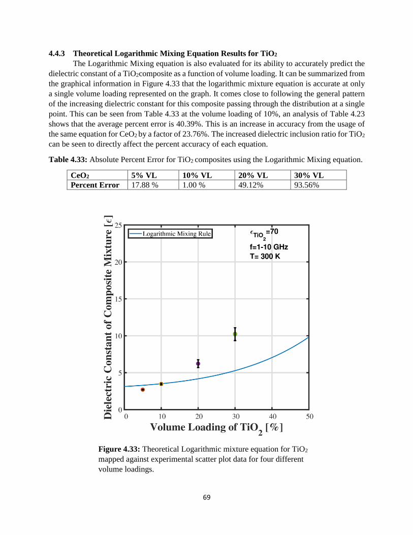
69
4.4.3 Theoretical Logarithmic Mixing Equation Results for TiO2
The Logarithmic Mixing equation is also evaluated for its ability to accurately predict the
dielectric constant of a TiO2composite as a function of volume loading. It can be summarized from
the graphical information in Figure 4.33 that the logarithmic mixture equation is accurate at only
a single volume loading represented on the graph. It comes close to following the general pattern
of the increasing dielectric constant for this composite passing through the distribution at a single
point. This can be seen from Table 4.33 at the volume loading of 10%, an analysis of Table 4.23
shows that the average percent error is 40.39%. This is an increase in accuracy from the usage of
the same equation for CeO2 by a factor of 23.76%. The increased dielectric inclusion ratio for TiO2
can be seen to directly affect the percent accuracy of each equation.
Table 4.33: Absolute Percent Error for TiO2 composites using the Logarithmic Mixing equation.
CeO2 5% VL 10% VL 20% VL 30% VL
Percent Error 17.88 % 1.00 % 49.12% 93.56%
Figure 4.33: Theoretical Logarithmic mixture equation for TiO2
mapped against experimental scatter plot data for four different
volume loadings.
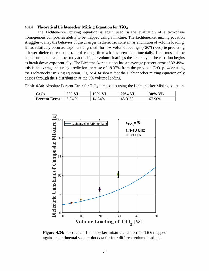
70
4.4.4 Theoretical Lichtenecker Mixing Equation for TiO2
The Lichtenecker mixing equation is again used in the evaluation of a two-phase
homogenous composites ability to be mapped using a mixture. The Lichtenecker mixing equation
struggles to map the behavior of the changes in dielectric constant as a function of volume loading.
It has relatively accurate exponential growth for low volume loadings (<20%) despite predicting
a lower dielectric constant rate of change then what is seen experimentally. Like most of the
equations looked at in the study at the higher volume loadings the accuracy of the equation begins
to break down exponentially. The Lichtenecker equation has an average percent error of 33.49%,
this is an average accuracy prediction increase of 19.37% from the previous CeO2 powder using
the Lichtenecker mixing equation. Figure 4.34 shows that the Lichtenecker mixing equation only
passes through the t-distribution at the 5% volume loading.
Table 4.34: Absolute Percent Error for TiO2 composites using the Lichtenecker Mixing equation.
CeO2 5% VL 10% VL 20% VL 30% VL
Percent Error 6.34 % 14.74% 45.01% 67.90%
Figure 4.34: Theoretical Lichtenecker mixture equation for TiO2 mapped
against experimental scatter plot data for four different volume loadings.
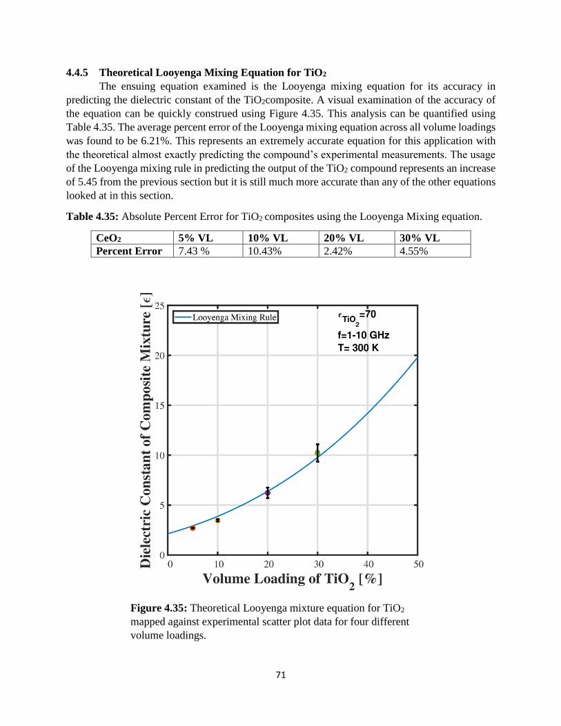
71
4.4.5 Theoretical Looyenga Mixing Equation for TiO2
The ensuing equation examined is the Looyenga mixing equation for its accuracy in
predicting the dielectric constant of the TiO2composite. A visual examination of the accuracy of
the equation can be quickly construed using Figure 4.35. This analysis can be quantified using
Table 4.35. The average percent error of the Looyenga mixing equation across all volume loadings
was found to be 6.21%. This represents an extremely accurate equation for this application with
the theoretical almost exactly predicting the compound’s experimental measurements. The usage
of the Looyenga mixing rule in predicting the output of the TiO2 compound represents an increase
of 5.45 from the previous section but it is still much more accurate than any of the other equations
looked at in this section.
Table 4.35: Absolute Percent Error for TiO2 composites using the Looyenga Mixing equation.
CeO2 5% VL 10% VL 20% VL 30% VL
Percent Error 7.43 % 10.43% 2.42% 4.55%
Figure 4.35: Theoretical Looyenga mixture equation for TiO2
mapped against experimental scatter plot data for four different
volume loadings.

72
4.4.6 Theoretical Birchak Mixing Equation for TiO2
Another evaluation of the CeO2 two-phase homogenous mixture equation’s is
accomplished using Birchak mixing equation the Birchak equation has an average percent error of
20.81%. Once again this can be seen in Figure 4.36, where the Birchak mixing equation using
varies outside of the t-distributions for all volume loadings. The Birchak equation does a good job
of predicting the growth of the dielectric constant of the mixture but overpredicts the value at each
of the measured points. At this higher dielectric inclusion ratio for TiO2 as compared to CeO2 the
Birchak mixing equation is less accurate with a decreased average accuracy of 13.73%.
Table 4.36: Absolute Percent Error for TiO2 composites using the Birchak Mixing equation.
CeO2 5% VL 10% VL 20% VL 30% VL
Percent Error 17.16% 24.98% 22.97% 18.15%
Figure 4.36: Theoretical Birchak mixture equation for TiO2
mapped against experimental scatter plot data for four different
volume loadings.
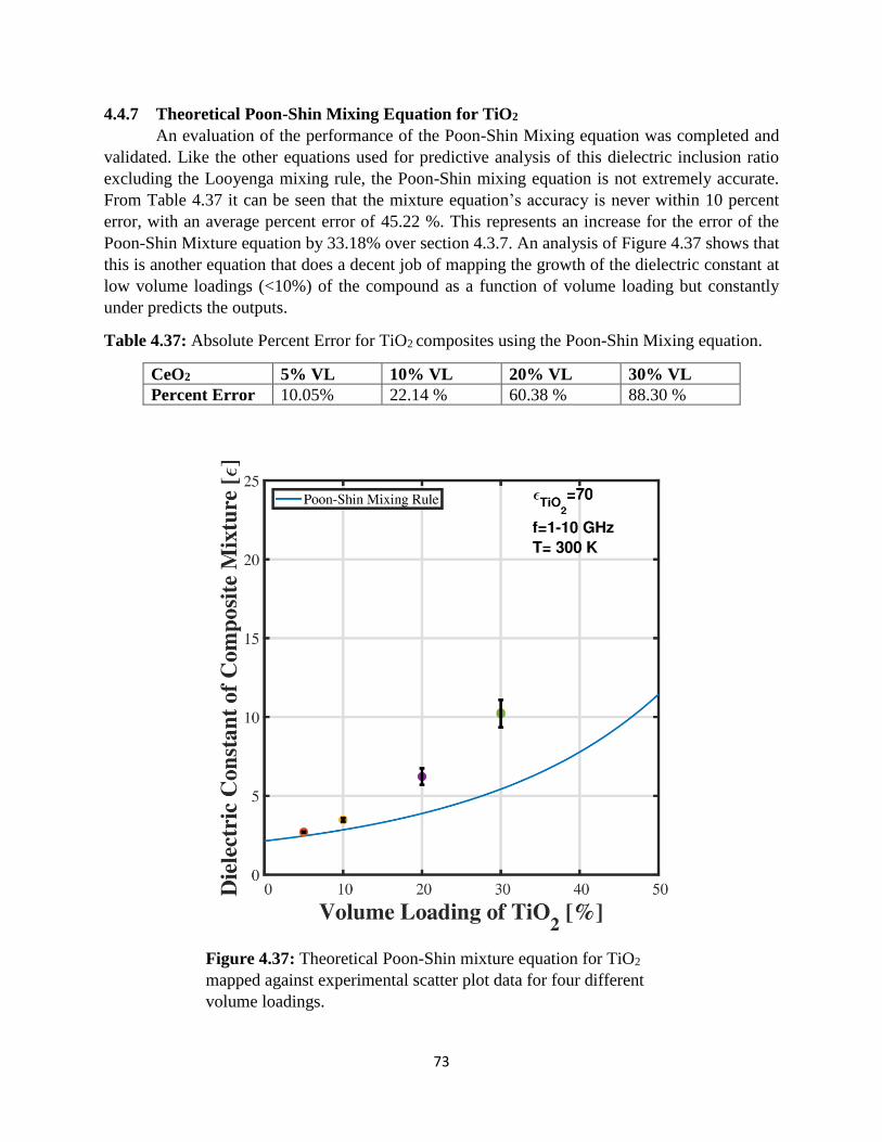
73
4.4.7 Theoretical Poon-Shin Mixing Equation for TiO2
An evaluation of the performance of the Poon-Shin Mixing equation was completed and
validated. Like the other equations used for predictive analysis of this dielectric inclusion ratio
excluding the Looyenga mixing rule, the Poon-Shin mixing equation is not extremely accurate.
From Table 4.37 it can be seen that the mixture equation’s accuracy is never within 10 percent
error, with an average percent error of 45.22 %. This represents an increase for the error of the
Poon-Shin Mixture equation by 33.18% over section 4.3.7. An analysis of Figure 4.37 shows that
this is another equation that does a decent job of mapping the growth of the dielectric constant at
low volume loadings (<10%) of the compound as a function of volume loading but constantly
under predicts the outputs.
Table 4.37: Absolute Percent Error for TiO2 composites using the Poon-Shin Mixing equation.
CeO2 5% VL 10% VL 20% VL 30% VL
Percent Error 10.05% 22.14 % 60.38 % 88.30 %
Figure 4.37: Theoretical Poon-Shin mixture equation for TiO2
mapped against experimental scatter plot data for four different
volume loadings.
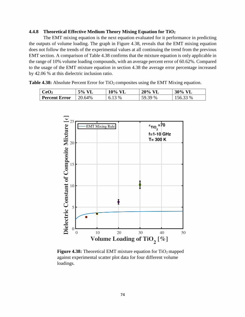
74
4.4.8 Theoretical Effective Medium Theory Mixing Equation for TiO2
The EMT mixing equation is the next equation evaluated for it performance in predicting
the outputs of volume loading. The graph in Figure 4.38, reveals that the EMT mixing equation
does not follow the trends of the experimental values at all continuing the trend from the previous
EMT section. A comparison of Table 4.38 confirms that the mixture equation is only applicable in
the range of 10% volume loading compounds, with an average percent error of 60.62%. Compared
to the usage of the EMT mixture equation in section 4.38 the average error percentage increased
by 42.06 % at this dielectric inclusion ratio.
Table 4.38: Absolute Percent Error for TiO2 composites using the EMT Mixing equation.
CeO2 5% VL 10% VL 20% VL 30% VL
Percent Error 20.64% 6.13 % 59.39 % 156.33 %
Figure 4.38: Theoretical EMT mixture equation for TiO2 mapped
against experimental scatter plot data for four different volume
loadings.
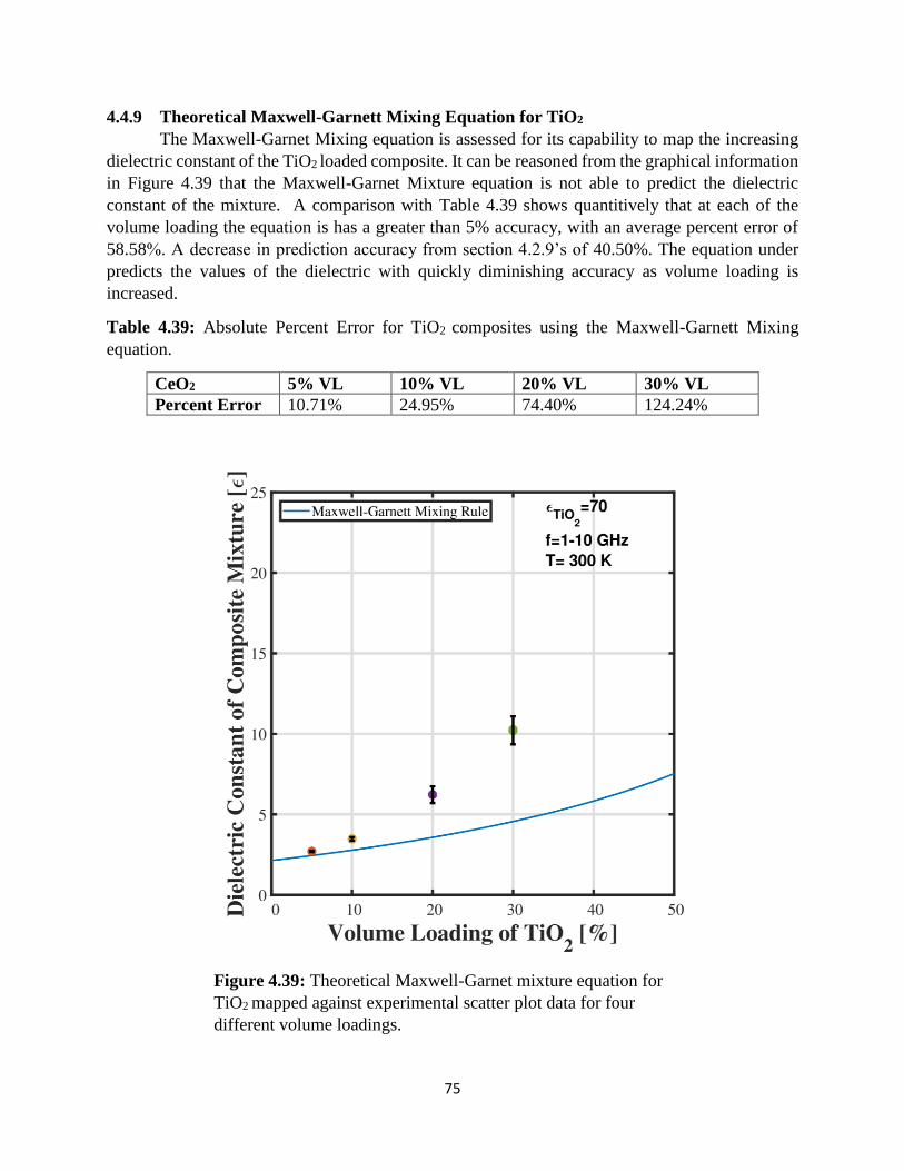
75
4.4.9 Theoretical Maxwell-Garnett Mixing Equation for TiO2
The Maxwell-Garnet Mixing equation is assessed for its capability to map the increasing
dielectric constant of the TiO2 loaded composite. It can be reasoned from the graphical information
in Figure 4.39 that the Maxwell-Garnet Mixture equation is not able to predict the dielectric
constant of the mixture. A comparison with Table 4.39 shows quantitively that at each of the
volume loading the equation is has a greater than 5% accuracy, with an average percent error of
58.58%. A decrease in prediction accuracy from section 4.2.9’s of 40.50%. The equation under
predicts the values of the dielectric with quickly diminishing accuracy as volume loading is
increased.
Table 4.39: Absolute Percent Error for TiO2 composites using the Maxwell-Garnett Mixing
equation.
CeO2 5% VL 10% VL 20% VL 30% VL
Percent Error 10.71% 24.95% 74.40% 124.24%
Figure 4.39: Theoretical Maxwell-Garnet mixture equation for
TiO2 mapped against experimental scatter plot data for four
different volume loadings.

76
4.4.10 Theoretical Jayasundere-Smith Mixing Equation for TiO2
The final equation analyzed in this section was the Jayasundere-Smith mixing equation.
Table 4.40 shows that the accuracy of the Looyenga mixing equation decreases steadily as volume
loading increases, like practically all the equations evaluated in this section. The Jayasundere-
Smith equation has an overall error of 32.33% across all volume loadings, an increase of 26.79%
from the previous powder. These results can be clearly clarified by a comparison with Figure 4.40,
where the mixture equation diverges from the measured values increasingly at high volume
loadings. For this higher dielectric inclusion ratio, the Jayasundere-Smith equation constantly
under predicts the value of the compound.
Table 4.40: Absolute Percent Error for TiO2 composites using the Jayasundere-Smith Mixing
equation.
CeO2 5% VL 10% VL 20% VL 30% VL
Percent Error 8.95% 17.57% 43.78% 59.13%
Figure 4.40: Theoretical Jayasundere-Smith mixture equation for
TiO2 mapped against experimental scatter plot data for four
different volume loadings.
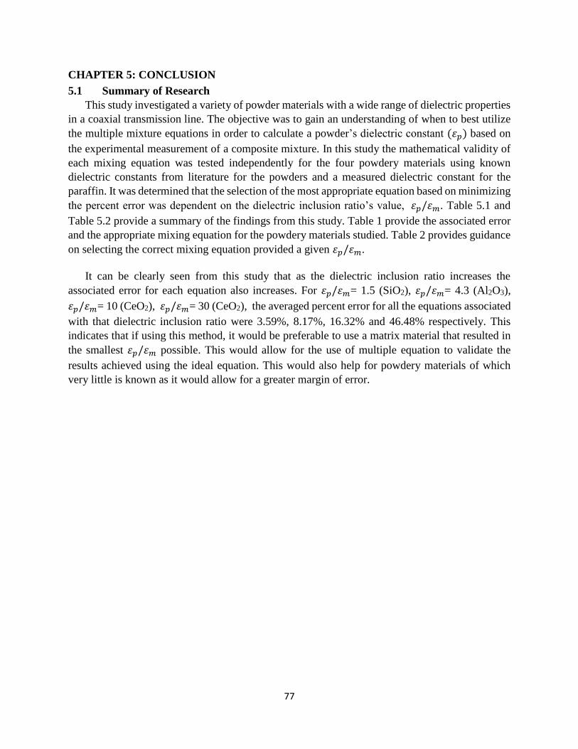
77
CHAPTER 5: CONCLUSION
5.1 Summary of Research
This study investigated a variety of powder materials with a wide range of dielectric properties
in a coaxial transmission line. The objective was to gain an understanding of when to best utilize
the multiple mixture equations in order to calculate a powder’s dielectric constant (휀𝑝) based on
the experimental measurement of a composite mixture. In this study the mathematical validity of
each mixing equation was tested independently for the four powdery materials using known
dielectric constants from literature for the powders and a measured dielectric constant for the
paraffin. It was determined that the selection of the most appropriate equation based on minimizing
the percent error was dependent on the dielectric inclusion ratio’s value, 휀𝑝/휀𝑚. Table 5.1 and
Table 5.2 provide a summary of the findings from this study. Table 1 provide the associated error
and the appropriate mixing equation for the powdery materials studied. Table 2 provides guidance
on selecting the correct mixing equation provided a given 휀𝑝/휀𝑚.
It can be clearly seen from this study that as the dielectric inclusion ratio increases the
associated error for each equation also increases. For 휀𝑝/휀𝑚= 1.5 (SiO2), 휀𝑝/휀𝑚= 4.3 (Al2O3),
휀𝑝/휀𝑚= 10 (CeO2), 휀𝑝/휀𝑚= 30 (CeO2), the averaged percent error for all the equations associated
with that dielectric inclusion ratio were 3.59%, 8.17%, 16.32% and 46.48% respectively. This
indicates that if using this method, it would be preferable to use a matrix material that resulted in
the smallest 휀𝑝/휀𝑚 possible. This would allow for the use of multiple equation to validate the
results achieved using the ideal equation. This would also help for powdery materials of which
very little is known as it would allow for a greater margin of error.
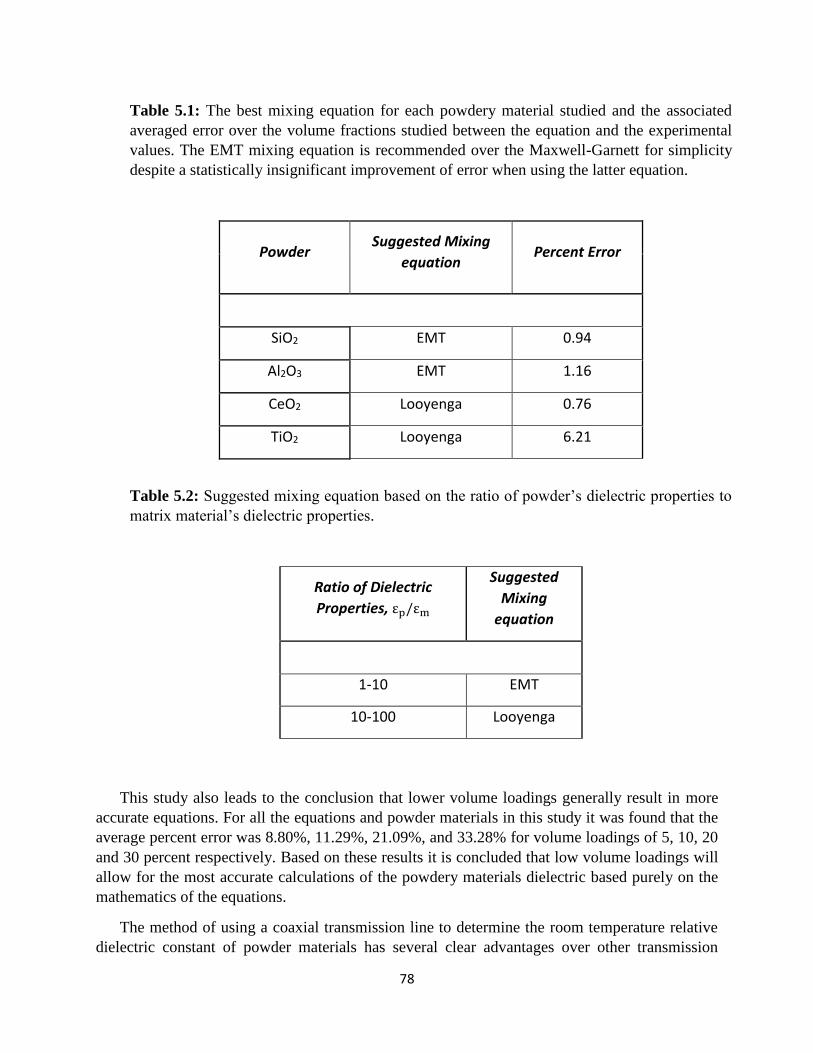
78
This study also leads to the conclusion that lower volume loadings generally result in more
accurate equations. For all the equations and powder materials in this study it was found that the
average percent error was 8.80%, 11.29%, 21.09%, and 33.28% for volume loadings of 5, 10, 20
and 30 percent respectively. Based on these results it is concluded that low volume loadings will
allow for the most accurate calculations of the powdery materials dielectric based purely on the
mathematics of the equations.
The method of using a coaxial transmission line to determine the room temperature relative
dielectric constant of powder materials has several clear advantages over other transmission
Table 5.1: The best mixing equation for each powdery material studied and the associated
averaged error over the volume fractions studied between the equation and the experimental
values. The EMT mixing equation is recommended over the Maxwell-Garnett for simplicity
despite a statistically insignificant improvement of error when using the latter equation.
Powder Suggested Mixing
equation Percent Error
SiO2 EMT 0.94
Al2O3 EMT 1.16
CeO2 Looyenga 0.76
TiO2 Looyenga 6.21
Table 5.2: Suggested mixing equation based on the ratio of powder’s dielectric properties to
matrix material’s dielectric properties.
Ratio of Dielectric
Properties, εp/εm
Suggested
Mixing
equation
1-10 EMT
10-100 Looyenga
.

79
methods. The approach has clear advantages over surface probe methods that are susceptible to
differential pressures and free space methods that required complicated calibration considerations,
to permit powdery materials that are electrically conductivity to be measured using a coaxial
method the powders were incorporating with non-conductive paraffin mixture. By keeping the
volume loading within the state range and forming coaxial plugs in the manor described within the
study, it is proposed that reliable dielectric measurements can be made with greater certainty than
other methods.
It was found during testing that several material and preparation factors helped to improve the
accuracy of the dielectric testing. Smaller particle sizes (<65 μm) were preferred for composite
preparations. Particle size of 30 μm had the best distribution within the paraffin matrix as well as
typically having the most accurate volume loadings. The smaller particle sizes helped to avoid any
particle clustering that would have interfered with the dielectric constant of the mixture.
To avoid airgaps between the sample and inner/outer conductor special attention had to be paid
to the effects of thermal expansion on the composites. As the paraffin composites cooled they
experienced an expansion away from the center probe mold and into the outer sleeve of the casting
mold. This resulted in the need to make the 3-D printed center conductor’s diameter smaller than
that of the actual conductor by 0.1 nm. Having the samples outer diameter be slightly larger than
that of the testing cell helped to ensure no airgaps existed between the sample and conducting
walls. Since paraffin in soft, inserting the sample into the test cell shaved off excess paraffin
resulted in a sample with the exact dimensions of the test cell.
5.2 Future Directions
This study looks to continue applying the methodology developed in the study of more
complex materials. The same methodology can be applied to powders that are frequency dependent
allowing for the same calculation to be done at each frequency of interest. This will allow for a
more robust usage of this methodology as most material’s dielectric constants are frequency
dependent. The study will also begin to look at magnetic materials using this same method of
paraffin-powder composites. Special work will have to be done to ensure no conglomeration of
particles during the curing process, but no significant changes will need to be made to
accommodate magnetic powders. Another direction of research will be high temperature dielectric
testing of powders, as most materials dielectric constants are temperature dependent as well as
frequency dependent.
80
References
(1) Sihvola, A. Electromagnetic Mixing Formulas and Applications; 1999.
(2) Musho, T. D.; Wildfire, C.; Houlihan, N. M.; Sabolsky, E. M.; Shekhawat, D. Study of
Cu2O Particle Morphology on Microwave Field Enhancement. Materials Chemistry and
Physics. 2018, pp 278–284. 2018
(3) Sphicopoulos, T.; Teodoridis, V.; Gardiol, F. Simple Nondestructive Method for the
Measurement of Material Permittivity. J. Microw. Power 1985, 20 (3), 165–172.
(4) Stuchly, M. A.; Stuchly, S. S. Coaxial Line Reflection Methods for Measuring Dielectric
Properties of Biological Substances at Radio and Microwave Frequencies—A Review. J.
Microw. Power 1980, 43 (3), 165–172.
(5) Baker-jarvis, J.; Janezic, M. D.; Domich, P. D.; Geyer, R. G. Analysis of an Open-Ended
Coaxial Probe with Lift-Off for Nondestructive Testing. 1994, 43 (5), 1–8.
(6) Wildfire, C.; Sabolsky, E. M.; Spencer, M. J.; Shekhawat, D. Solid-State Synthesis of YAG
Powders through Microwave Coupling of Oxide/Carbon Particulate Mixtures. Ceramics
International. 2017, pp 11455–11462. 2017
(7) Chung-Lun, L.; Jenq-Gong, D.; Bi-Shiou, C.; Wen-Hsi, L. Low-Temperature Sintering and
Microwave Dielectric Properties of Anorthite-Based Glass-Ceramics. J. Eur. Ceram. Soc.
2002, 95 (8), 2230–2235.
(8) Alford, N. M. N.; Penn, S. J. Sintered Alumina with Low Dielectric Loss. J. Appl. Phys.
1996, 80 (10), 5895–5898.
(9) Higasi, K. Dielectric Investigation on Coals. II. Mixture of Coal Powder and Paraffin Wax.
1957, 30 (5), 546.
(10) Dionne, G. F.; Fitzgerald, J. F.; Aucoin, R. C. Dielectric Constants of Paraffin-Wax-TiO2
Mixtures. J. Appl. Phys. 1976, 47 (4), 1708–1709.
(11) Kelly, J. M.; Stenoien, J. O.; Isbell, D. E. Wave-Guide Measurements in the Microwave
Region on Metal Powders Suspended in Paraffin Wax. J. Appl. Phys. 1953, 24 (3), 258–
262.
(13) GNU Free Documentation Licese, Version 1.2, Free Software Foundation. 2019
(12) Vainshtein, L. A. Electromagnetic Waves. Izd. Radio i Sviaz 1988, 00, 440.
(14) Purcell, E. M. Electricity and Magnetism, Second.; McGraw-Hill Book Company: New
York, 1985.
(15) Horikoshi, S.; Schiffmann, R. F.; Fukushima, J.; Serpone, N. Microwave Chemical and
Materials Processing: A Tutorial; 2017.
(16) Stuerga, D. Microwave-Material Interactions and Dielectric Properties, Key Ingredients
for Mastery of Chemical Microwave Processes; 2008; Vol. 1.
81
(17) Surati, M. A.; Jauhari, S.; Desai, K. R. A Brief Review : Microwave Assisted Organic
Reaction. Arch. Appl. Sci. Res. 2012, 4 (1), 645–661.
(18) Fung, A. K.; Chen, K.-S.; Schutzer, and D. Microwave Scattering and Emission Models
for Users, 1st ed.; Artech House: Norwood, 2010.
(19) Zangwill, A. Modern Electrodynamics; 2013.
(20) Katrib, J.; Folorunso, O.; Dodds, C.; Dimitrakis, G.; Kingman, S. W. Improving the Design
of Industrial Microwave Processing Systems through Prediction of the Dielectric Properties
of Complex Multi-Layered Materials. J. Mater. Sci. 2015.
(21) Sugawara, H.; Kashimura, K.; Hayashi, M.; Matsumuro, T.; Watanabe, T.; Mitani, T.
Temperature Dependence and Shape Effect in High-Temperature Mi- Crowave Heating of
Nickel Oxide Powders. Phys. B Phys. Condens. Matter 2015, 458, 35–39.
(22) Mishra, R. R.; Sharma, A. K. Microwave-Material Interaction Phenomena: Heating
Mechanisms, Challenges and Opportunities in Material Processing. Composites Part A:
Applied Science and Manufacturing. 2016, pp 78–97.
(23) Bartley, P. G.; Begley, S. B. A New Technique for the Determination of the Complex
Permittivity and Permeability of Materials. 2010 IEEE Int. Instrum. Meas. Technol. Conf.
I2MTC 2010 - Proc. 2010, 54–57.
(24) Arthur R. Von Hipple. Dielectric Materals and Applications; Arthur R. Von Hipple, Ed.;
The MIT Press, 1952.
(25) Arthur R. Von Hipple, S. Ramo, J. R. W. Dielectrics and Waves. Fields and Waves in
Mordern Radio 1955, 8 (2).
(26) Geyer, R. G.; Grosvenor, C. A.; Holloway, C. L.; Janezic, M. D.; Johk, R. T.; Kabos, P.;
Baker-Jarvis, J. Measuring the Permittivity and Permeability of Lossy Materials :; 2005.
(27) Hashin, Z.; Shtrikman, S. A Variational Approach to the Theory of the Effective Magnetic
Permeability of Multiphase Materials. J. Appl. Phys. 1962, 33 (10), 3125–3131.
(28) Ebara, H.; Inoue, T.; Hashimoto, O. Measurement Method of Complex Permittivity and
Permeability for a Powdered Material Using a Waveguide in Microwave Band. Sci.
Technol. Adv. Mater. 2006, 7 (1 SPEC. ISS.), 77–83.
(29) Blakney, T. L.; Weir, W. B. Automatic Measurement of Complex Dielectric Constant and
Permeability at Microwave Frequencies. Proc. IEEE 1975, 63 (1), 203–205.
(30) Choy, T. C. Effective Medium Theory: Principles and Applications, 2nd ed.; Oxford
University Press, 2015.
(31) Anderson, R. W. S-Parameter Techniques For Faster, More Accurate Network Design;
1967.
(32) Agilent Technologies. Advanced Design System 1.5 Circuit Simulatione; Palo Alto, 2000.
(33) Jilani, M. T.; Rehman, M. Z. ur; Khan, A. M.; Khan, M. T.; Ali, S. M. A Brief Review of
Measuring Techniques for Characterization of Dielectric Materials. Int. J. Inf. Technol.
82
Electr. Eng. 2012, 1 (1), 1–5.
(34) Venkatesh, M. S.; Raghavan, G. S. V. An Overview of Dielectric Properties Measuring
Techniques. J. Can. Soc. Bioeng. 2005, 47 (40), 7.15-7.30.
(35) Yaw, K. C. Measurement of Dielectric Material Properties Application Note, Rohde &
Schwarz. Meas. Tech. 2006, 1–35.
(36) Technologies, K. N5231A PNA-L Microwave Network Analyzer, 13.5 GHz
(37) Bussey, H. E. Measurement of RF Properties of Materials A Survey. Proc. IEEE 1967, 55
(6).
(38) Busseyt, H. E. Measurement and Standardization of DieIectric Sam&; 1962, No. 4, 4–7.
(39) Nicolson, A. M.; Ross, G. F. Measurement of the {Intrinsic} {Properties} of {Materials}
by {Time}-{Domain} {Techniques}. IEEE Trans. Instrum. Meas. 1970, 19 (4), 377–382.
(40) Agilent Technologies. Models in the 85071E Materials Measurement Software.
(41) Baker-Jarvis, J.; Janezic, M. D.; Grosvenor Jr, J. H.; Geyer, R. G. Transmission/Reflection
and Short-Circuit Line Methods for Measuring Permittivity and Permeability; OFFICE, U.
S. G. P., Ed.; Washington D.C., 1992.
(42) Catalá-civera, J. M.; Member, S.; Canós, A. J.; Plaza-gonzález, P.; Gutiérrez, J. D.; García-
baños, B.; Peñaranda-foix, F. L.; Member, S. Dynamic Measurement of Dielectric
Properties of Materials at High Temperature During Microwave Heating in a Dual Mode
Cylindrical Cavity. 2015, 63 (9), 2905–2914.
(43) Thommes, M.; Shields, J. E.; Thomas, M. A. Characterization of Porous Solids and
Powders: Surface Area, Pore Size and Density, 1st ed.; Shields, J. E., Thomas, M. A.,
Lowell, S., Eds.; Springer Science & Buisness Media, 2004.
(44) Castellanos, A. The Relationship between Attractive Interparticle Forces and Bulk
Behaviour in Dry and Uncharged Fine Powders; 2005; Vol. 54.
(45) Javanbakht, M.; Salahinejad, E.; Hadianfard, M. J. The Effect of Sintering Temperature on
the Structure and Mechanical Properties of Medical-Grade Powder Metallurgy Stainless
Steels. Powder Technol. 2016, 289, 37–43.
(46) Ahmad, S. I.; Koteshwar Rao, P.; Syed, I. A. Sintering Temperature Effect on Density,
Structural and Morphological Properties of Mg- and Sr-Doped Ceria. J. Taibah Univ. Sci.
2016, 10 (3), 381–385.
(47) Sandi, D.; Supriyanto, A.; Jamaluddin, A.; Iriani, Y. The Effects of Sintering Temperature
on Dielectric Constant of Barium Titanate (BaTiO3). IOP Conf. Ser. Mater. Sci. Eng. 2016,
107 (1), 1–7.
(48) Costa, A. M. L. M.; Baroni, D. B.; Lucas, C. S.; Bittencourt, M. S. Q. ULTRASONIC
ANALYSIS OF SINTERED ALUMINA PELLETS. 2016, No. May.
(49) Vattur Sundaram, M. Processing Methods for Reaching Full Density Powder Metallurgical
Materials. 2017, 39.
83
(50) Donachie Jr., M. J.; Burr, M. F. Effects of Pressing on Metal Powders. J. Met. 1963, 14,
849–850.
(51) Essa, K.; Jamshidi, P.; Zou, J.; Attallah, M. M.; Hassin, H. Porosity Control in 316L
Stainless Steel Using Cold and Hot Isostatic Pressing. Mater. Des. 201AD, 138 (15), 21–
29.
(52) Taylor, P.; Himran, S.; Suwono, A.; Mansoori, G. A. L. I. Characterization of Alkanes and
Paraffin Waxes for Application as Phase Change Energy Storage Medium Characterization
of Alkanes and Paraf ’ Fin Waxes for Application as Phase Change Energy Storage
Medium. 1994, 16 (August 2014), 37–41.
(53) Gasia, J.; Miró, L.; de Gracia, A.; Barreneche, C.; Cabeza, L. F. Experimental Evaluation
of a Paraffin as Phase Change Material for Thermal Energy Storage in Laboratory
Equipment and in a Shell-and-Tube Heat Exchanger. Appl. Sci. 2016, 6 (5).
(54) Chen, W. S.; Hsieh, M. Y. Dielectric Constant Calculation Based on Mixture Equations of
Binary Composites at Microwave Frequency. Ceram. Int. 2017.
(55) Sihvola, A. Mixing Rules with Complex Dielectric Coefficients. Subsurf. Sens. Technol.
Appl. 2000, 1 (4), 393–515.
(56) Simpkin, R. Derivation of Lichtenecker’s Logarithmic Mixture Formula from Maxwell’s
Equations. IEEE Trans. Microw. Theory Tech. 2010, 58 (3), 545–550.
(57) Poon, Y. M.; Shin, F. G. A Simple Explicit Formula for the Effective Dielectric Constant
of Binary 0-3 Composites. J. Mater. Sci. 2004, 39 (4), 1277–1281.
(58) Mallet, P.; Guérin, C. A.; Sentenac, A. Maxwell-Garnett Mixing Rule in the Presence of
Multiple Scattering: Derivation and Accuracy. Phys. Rev. B - Condens. Matter Mater. Phys.
2005, 72 (1), 1–9.
(59) Tuhkala, M.; Juuti, J.; Jantunen, H. Method to Characterize Dielectric Properties of
Powdery Substances. J. Appl. Phys. 2013, 114 (1).
(60) Jayasundere, N.; Smith, B. V. Dielectric Constant for Binary Piezoelectric 0-3 Composites.
J. Appl. Phys. 1993, 73 (5), 2462–2466.
(61) Sigma-Aldrich. SiO2, 2017
(62) Samsonov, G. V. The Oxide Handbook, 2nd ed.; New York, 1982.
(63) Inframat. Al2O3, 2016
(64) Hayat, A.; Andreescu, D.; Bulbul, G.; Andreescu, S. Redox Reactivity of Cerium Oxide
Nanoparticles against Dopamine. J. Colloid Interface Sci. 2014, 418, 240–245.
(65) Scientific, F. Titanium(IV) oxide, AeroxideTM P25, ACROS OrganicsTM , 2017
(66) Schindelin, J.; Arganda-Carreras, I.; Frise. Fiji: An Open-Source Platform for Biological-
Image Analysi. Nat. Methods 2012, 9 (7), 676–682.
(67) Mauritz, K. Dielectric Spectroscopy. PSRC.edu, 2012
84
(68) Smiths Interconnect. Linear-circular Polarizers and Circular-to-rectangular Waveguide,
2017