experimental quantification of the seismoelectric transfer ... · pdf filethe documents may...
TRANSCRIPT

HAL Id: hal-01386943https://hal.archives-ouvertes.fr/hal-01386943
Submitted on 24 Oct 2016
HAL is a multi-disciplinary open accessarchive for the deposit and dissemination of sci-entific research documents, whether they are pub-lished or not. The documents may come fromteaching and research institutions in France orabroad, or from public or private research centers.
L’archive ouverte pluridisciplinaire HAL, estdestinée au dépôt et à la diffusion de documentsscientifiques de niveau recherche, publiés ou non,émanant des établissements d’enseignement et derecherche français ou étrangers, des laboratoirespublics ou privés.
Distributed under a Creative Commons Attribution - NonCommercial - ShareAlike| 4.0International License
Experimental quantification of the seismoelectrictransfer function and its dependence on conductivity
and saturation in loose sandJulia Holzhauer, Daniel Brito, Clarisse Bordes, Yèble Brun, Bertrand
Guatarbes
To cite this version:Julia Holzhauer, Daniel Brito, Clarisse Bordes, Yèble Brun, Bertrand Guatarbes. Experimental quan-tification of the seismoelectric transfer function and its dependence on conductivity and saturationin loose sand. Geophysical Prospecting, Wiley, 2016, 000, pp.0 - 0. <10.1111/1365-2478.12448>.<hal-01386943>

Geophysical Prospecting (0000) 000, 000–000
Experimental quantification of the seismoelectric transfer functionand its dependence on conductivity and saturation in loose sand
J. Holzhauer, D. Brito, C. Bordes, Y. Brun and B. GuatarbesUniv. Pau & Pays Adour, CNRS, TOTAL - UMR 5150 - LFC-RLaboratoire des Fluides Complexes et leurs RéservoirsBP 1155 - PAU, F-64013, France
[email protected],[email protected],[email protected],[email protected],[email protected]
24 October 2016

2 J. Holzhauer et al.
SUMMARYUnder certain circumstances, seismic propagation within porous media may be associated toa conversion of mechanical into electromagnetical energy known as a seismoelectromagneticphenomemon. The propagation of fast compressional P -waves is more specifically associatedto manifestations of a seismoelectric field linked to fluid flow within the pores. The analysisof seismoelectric phenomena, which requires combining the theory of electrokinetics to Biot’stheory of poroelasticity, provides us with a transfer function noted E/u that links the coseismicseismoelectric field E to the seismic acceleration u. In order to measure the transfer function,we have developed an experimental set-up enabling seismoelectric laboratory observation inunconsolidated quartz sand within the kilohertz range. The investigation focused on the im-pact of fluid conductivity and water saturation over the coseismic seismoelectric field. Duringthe experiment, special attention was given to the accuracy of electric field measurements. Weconcluded that, in order to obtain a reliable estimate of the electric field amplitude, the dipolefrom which the potential differences are measured should be of much smaller length than thewavelength of the propagating seismic field. Time-lapse monitoring of the seismic velocitiesand seismoelectric transfer functions were performed during imbibition and drainage experi-ments. In all cases, the quantitative analysis of the seismoelectric transfer function E/u was ingood agreement with theoretical predictions. While investigating saturation variations from theresidual water saturation to full saturation, we showed that the E/u ratio undergoes a switchin polarity at a particular saturation S∗, also implying a sign change of the filtration, traduc-ing a reversal of the relative fluid displacement with respect to the frame. This sign change atcritical saturation S∗ stresses a particular behaviour of the poroelastic medium: the droppingof the coseismic electric field to zero traduces the absence of relative pore/fluid displacementsrepresentative of a Biot dynamically compatible medium. We concluded from our experimentalstudy in loose sand that measurements of the coseismic seismoelectric coupling may provideinformation on fluid distribution within the pores, and that the reversal of the seismoelectricfield may be used as an indicator of the dynamically compatible state of the medium.

Experimental quantification of the seismoelectric transfer function 3
Key words: Seismics, Monitoring, Reservoir Geophysics, Acoustics, Electromagnetics

4 J. Holzhauer et al.
1 INTRODUCTION
Seismoelectromagnetic effects may be observed when a seismicwave propagates within a porous medium formed from a solidframe filled with a fluid of low to moderate electrical conductiv-ity.Under such conditions, an electrical double layer forms at themineral-solution interface due to cations adsorption, thus enablingthe setting of an electrokinetic coupling. The mechanically drivenmovements of the electrolyte relatively to the frame consequentlyresult in a charge separation, producing a propagating electromag-netic (EM) field said to be "coseismic". According to the nature ofthe original seismic excitation, the propagating coseismic field maybe overwhelmingly electric or magnetic; P-waves for instance areusually associated to coseismic seismoelectric (SE) fields. In anycases, seismoelectromagnetic manifestations will propagate simi-larly to the supporting seismic wave and will be affected by theproperties - of either hydraulic, mechanical or electrical nature -characterizing the medium in its close vicinity. When the incidentacoustic wave meets a discontinuity affecting the pore space in anygeometrical or chemical manner (should it be a change in matrixdensity or a brutal variation of fluid conductivity), seismoelectro-magnetic effects of a second kind, referred to as "interfacial" andpropagating at EM-speed, might be generated. Such effects havebeen reported at field scale (Haines et al. 2007; Dupuis et al. 2007)and mesoscopic scale (Jougnot et al. 2013; Monachesi et al. 2015;Grobbe & Slob 2016). Note that as any physical coupling, seismo-electrics has a counter-effect known as electroosmosis, in which theapplication of an EM field induces a seismic propagation within aporous medium (Jouniaux & Zyserman 2016). This phenomenonwas first reproduced at field-scale by Thompson & Gist (1993) be-fore being observed at lab-scale by Zhu et al. (1999).
The possibility of combining seismic and electric surveys(electric field monitoring during seismic excitation) has been ad-dressed as early as the 1930s. Following observations by Blau &Statham (1936), Thompson (1936) suggested using their combi-nation as an exploration tool (producing what he refers to as theseismic-electric effect). A few years later Ivanov (1939, 1940), hav-ing run similar experiments in the field, suspected the observed sig-nals to result from an electrokinetic coupling effect that he calledseismic-electric effect of the second kind in distinction to piezo-electricity.
Frenkel (1944), attempted to develop a quantitative theory toexplain Ivanov’s observations. He formulated the first complete setof equations governing the acoustics of isotropic porous media. Yetit was Biot who, a decade later, achieved the first fully valid theoryof poroelasticity. Biot (1956a,b) divided his treatment of the lin-ear theory of porous media acoustics into two distinct frequency-domains, delimited with regard to the validity of Poiseuille flowassumption by introducing the Biot critical frequency fBiot. Hestated the existence of one rotational (S − type) and two dilata-tional (P − type) waves, subsequently referred to as P − fastand P − slow, the latter being highly dispersive and diffusive. Ina later paper Biot (1962) would emphasize the role this slow wavecould play in electrokinetics, as it enhances fluid velocity within thepores. The next theoretical step to couple Biot’s theory with elec-trokinetics while accounting for Onsager’s reciprocity was taken byNeev & Yeatts (1989). Yet, in accordance with Frenkel’s approach,they did not consider the full set of Maxwell’s equation, leadingthem to ignore seismomagnetic effect. The breakthrough of seis-moelectromagnetics was finally enabled by Pride’s formulation ofthe underlying theory.
The theoretical background for seismoelectromagnetic phe-
nomena was proposed by Pride (1994) as a set of equations basedon Biot’s original theory including the electrokinetic coupling aswell as Maxwell’s equations. In the light of this complete theory,the first dynamic transfer functions for the coseismic seismoelectricfield were proposed a few years later by Pride & Haartsen (1996)for both transverse and longitudinal waves. Using low-frequencyassumptions, Garambois & Dietrich (2001) proposed a linear ex-pression linking the coseismic electric field to seismic accelera-tion of P -waves, applicable in particular to field measurementsat seismic frequencies. Lately, seismic interferometry methods us-ing Green functions (Wapenaar et al. 2006; Wapenaar & Fokkema2006; Slob & Wapenaar 2007) have been adapted to provide the im-pulsive seismoelectric response of the porous medium equivalent tousual transfer functions. This method was first implemented for in-terfacial (Wapenaar et al. 2008; De Ridder et al. 2009) and coseis-mic (Schoemaker et al. 2012) seismoelectric before being extendedby Gao & Hu (2010) to the seismomagnetic aspects.
Pride’s theory being originally formulated for a fully-saturatedporous medium, its adaptation to partially saturated conditions con-stitutes an important development offering new perspectives. WhileBiot’s poroelasticity relations may be adjusted by defining effec-tive fluid properties (Wood 1955; Teja & Rice 1981; Brie et al.1995), saturation-dependence of electrokinetics is still discussed. Ithas been the subject of numerous theoretical developments initiallyproposed for the continuous spontaneous potential, some based onvolume-averaging methods (Linde et al. 2007; Revil et al. 2007)others on capillary models (Jackson 2008, 2010), the former high-lighting the role of the electrolyte wettability while the latter fo-cuses on the thickness of the electrical double layer. Yet, to ac-count for experimental observations, further empirical laws are of-ten required (Guichet et al. 2003; Allègre et al. 2012). Eventually,the question of partial saturation has been directly broached undera seismoelectric angle either based on Pride’s classical approach(Warden et al. 2013), or on an alternative reformulation using elec-trokinetic couplings as a function of charge density (Revil & Jar-dani 2010; Revil & Mahardika 2013; Revil et al. 2013).
The first seismoelectric laboratory experiments dealt withthe impact of fluid properties on seismoelectric observations(Parkhomenko et al. 1964; Parkhomenko 1971; Parkhomenko &Gaskarov 1971). These types of laboratory experiments were even-tually resumed by Ageeva et al. (1999) who introduced additionalfrequency variations. They observed at various frequencies that theratio of the electric field to the liquid-phase pressure changed di-rectly with water content and residual saturation on the one hand,and inversely with salinity, porosity and permeability on the other.In the meanwhile, an innovative laboratory apparatus of boreholegeometry, involving Stoneley waves, enabled to observe coseis-mic and interfacial seismoelectric signals as well as electroosmo-sis (Zhu et al. 1999). On their borehole laboratory model, Zhu& Toksöz (2005) finally reported the observation of seismomag-netic coseismic signals using a Hall-effect sensor. Contemporane-ously, quantitative measurements led by Bordes (2005) in an un-derground low-noise laboratory confirmed experimentally the ex-istence of the coseismic seismomagnetic field and its dependenceon shear-waves, as predicted by Pride’s theory (Bordes et al. 2006,2008).
After Zhu et al. (2000) and Zhu & Toksöz (2003) had inves-tigated experimentally the dependence of coseismic electric am-plitudes to fluid conductivity, Block & Harris (2006) confirmedthe expected tendency of electric amplitudes to diminish with in-creasing conductivity on a sand column experiment. Finally Zhu& Toksöz (2013) conducted extensive and quantitative dynamic

Experimental quantification of the seismoelectric transfer function 5
measurements of seismoelectric coupling coefficients under vary-ing conductivities (0.1 − 0.3 S · m−1): the seismoelectric cou-pling would decrease with increasing conductivity and increasingfrequency. According to recent extensive measurements by Bordeset al. (2015) regarding the dependence of the coseismic seismo-electric signal on water saturation within the range [0.3 − 0.9], theseismoelectric ratio E/u showed a rather stable behaviour, despitelarge saturation changes expected to induce correspondingly largevariations of the medium bulk conductivity.
Hence, in spite of its electrokinetic nature, seismoelectric ef-fects have generally been expected to show some aptitudes for hy-draulic characterization of porous media (Revil et al. 2015). Con-sequently, as part of the developing geophysical methods, seismo-electrics may eventually become a tool for reservoir characteriza-tion combining seismic and electric imaging abilities. Such per-spective requires a comprehensive understanding of the underlyingphenomena and their dependence to the involved medium param-eters, as well as the preliminary development of a reliable quan-titative measuring procedure. With this prospect, the goal of thepresent study is to perform quantitative measurements of the co-seismic seismoelectric field for comparison to theoretical predic-tions, that is the study of the dynamic transfer function E/u.
Following the fundamental studies by Pride (1994) and Pride& Haartsen (1996), developments by Warden et al. (2013) and Bor-des et al. (2015) extended the original formulation of the seismo-electric dynamic transfer function, initially written for saturatedmedia, to partially saturated states. This step was taken by introduc-ing the model for electrokinetic coupling dependence on saturationdeveloped by Jackson (2010), along with a mechanical characteri-zation of the biphasic fluid as a bulk effective fluid (the first topichas been discussed by Bordes et al. (2015), while the second willbe more largely exposed in this article). This led to the relation be-tween the acceleration u due to fast P -waves, and its associatedcoseismic electric field E:
E
u(ω, Sw, σf , . . .) = i
ρL
ωε
Hs2 − ρCs2 − ρf
(1)
where ω is the angular frequency, Sw is the water saturation, σf isthe fluid conductivity, ρ is the effective density, L is the dynamicseismoelectric coupling coefficient, ε is the effective electric per-mittivity, H and C are poroelastic moduli of the medium, s is theslowness of the fast compressional P -wave, ρ is the bulk density ofthe porous medium and ρf is the effective fluid density. For the sakeof clarity, the parameters dependence as a function of (ω, Sw, . . . )is not explicitly written on the right hand side of eq. (1). Note thatthe original seismoelectric transfer function and the electrokineticadjustment to partial saturation resulting in eq. (1) were both basedon the assumption of an electrical double layer much thinner thanthe pore section (Pride 1994).
As detailed in Bordes et al. (2015), we considered thefrequency-dependent transfer function E/u as expressed in eq. (1)to depend on several parameters of the medium: some of themare related to the fluid phase, others depend on the solid phaseand finally further parameters characterize the frame. Our presentpurpose is to quantitatively evaluate E/u in a medium where theparameters can be inferred, either from direct experimental mea-surements or from theoretical estimations. We have therefore cho-sen to develop a metric sandbox experiment after initial works byBarrière et al. (2012) and Bordes et al. (2015). With its moderatepropagation velocity under sub-saturated conditions and a granu-lar matrix easily described by models, unconsolidated quartz sandappears particularly adapted to our purpose (Holzhauer 2015). Yet,
from a practical point of view, wavelengths being decimetric in sub-saturated sand will grow metric in a fully-saturated medium. Thecharacteristics of the experiment, as well as the physical propertiesof the sand are described in Part 2.
With all parameters of the medium involved in eq. (1) beingreasonably known, our quantification attempt of the coseismic seis-moelectric transfer function further requires high accuracy in accel-eration u and electric field E measurements at any given point ofthe sandbox. In this prospect, we have used calibrated accelerome-ters, and combined their results to those obtained on appropriatelyreconstructed dipoles which geometry is described in Part 3. Goodknowledge of the sand physical parameters coupled to a reliablemeasurements routine will provides us with a precise estimation ofthe ratio E/u for a given set of parameters during an experiment.
In order to validate our experimental approach in Part 4, wecompare our measurements to theoretical predictions while vary-ing the fluid conductivity σf , a key parameter for the amplitudeof E/u, the other parameters remaining roughly constant through-out the experiments. Having concluded to the agreement betweenmeasurements and model predictions, we vary a more challengingparameter regarding experimental conditions, namely water satura-tion Sw. Related imbibition and drainage experiments are reportedin Part 5. Part 6 eventually summarizes our results and concludeson our quantitative approach of the dynamic transfer function.

6 J. Holzhauer et al.
2 A MONITORED SEISMOELECTRIC EXPERIMENT
2.1 Description of the global set-up
We conceived a cubic sandbox from sealed plywood elements; ahole disposed on one side of the box allows the punch of a pneu-matic seismic source to pass through. The inside is accessible bythe open top. We arranged 3 cm-thick acoustic foam slabs at thebottom as well as on the opposed and lateral walls to the source inorder to prevent boundary reflection effects. The dimension of thesandbox is 53 × 50 cm2. It is filled with a 50 cm high sand-layer;the emission point of the seismic source is located at the center ofa 50 × 50 cm2 panel. Four injection wells placed at each cornerof the sandbox allow for bottom imbibition. These wells are con-nected to elevated water barrels in an attempt to improve saturationdegree by an increased water column. The average quantity of wa-ter required for initial imbibition would range by 60 liters. A globalview of the experiment is given in Fig. 1a).
[Figure 1 about here.]
Since preliminary seismoelectric measurements demonstratedthat the coseismic seismoelectric E field would be barely assess-able for offsets much larger than 20 cm, all our captors were placedwithin a distance of 30 cm to the source. By this choice of offsets,we notably differed from previous seismic (Barrière et al. 2012)and seismoelectric (Bordes et al. 2015) laboratory analysis. Whileenabling high captor density (20 accelerometers within a maxi-mal distance of 30 cm to the source), this receiver distribution re-quired disposing the transducers on two parallel lines. A thin cen-tral space, aligned with the source, was left free to host an elec-trode array of 30 electrodes created in agreement with the specificoffset-requirements. On this central line, electrodes were placed be-tween offsets of 3 cm and 30 cm. Accelerometers were implantedon either side of this central line with a centimetric lateral offset assketched in Fig. 2. Each accelerometer was systematically placedin regard to an electrode (see Fig. 1b) and Fig. 2). The sandbox wasfurther equipped with moisture sensors surrounding the measure-ment line, with the purpose of recollecting saturation information.
[Figure 2 about here.]
2.2 The porous medium
The loose sand we used in our experiment is the same material asthe one presented in the studies by Barrière et al. (2012) and Bor-des et al. (2015): namely pure silica sand (SiO2 content superiorto 98%) showing unidisperse granulometry of 250 µm and graindensity around 2635− 2660 kg ·m−3. While hydraulic properties(as porosity, formation factor and permeability) were directly mea-sured on small sand probes, other parameters, of electrical or me-chanical nature, have been inferred from models or previous stud-ies. The whole set of parameters and properties used in the presentstudy is listed in Table 1 and follows the notations defined in ap-pendices A and B from Bordes et al. (2015).
We estimated the zeta potential ζ, a parameter characterizingthe electrical double layer, by extrapolating an experimental obser-vation while using a ζ model depending on concentration C0. Onthe one hand, Pride & Morgan (1991) showed the dependence ofζ vs log(C0) to be linear, referring to various laboratory measure-ments in quartz sands. We then noticed that the slopes obtainedfrom the different datasets were close to an averaged value of about0.026mV.l.mol−1 whereas the ζ(0) seemed to be a specific prop-erty of the medium. On the other hand, measurements by Nazarova-
Cherrière (2014) showed the zeta potential in saturated Landes sandto be ζ = −35 mV (NaCl electrolyte, σf ' 8.8 mS.m−1). Even-tually, we used the relation ζ(C0) = 0.044+0.026 logC0 (inmV )obtained by combining both model and measurements (see Table 1for details).
[Table 1 about here.]
2.3 Pneumatic seismic source
The home-made pneumatic source was specifically designed to in-vestigate the frequency range for which the medium should be mostaffected by Biot’s losses, corresponding to the vicinity of the Biotfrequency:
fBiot =φηf
2πγ0ρfk0(2)
estimated at approximately 2 kHz under sub-saturated conditions.In eq. (2) φ, γ0, k0 are respectively the porosity, the tortuosity andthe permeability of the porous medium, while ηf and ρf stand cor-respondingly for the viscosity and density of the effective fluid.This source was made of a piston supplied with compressed air forone part, and a fixed frame that maintains the steel hitting plate byfour screws equipped with shock-absorbers for another part (seeFig. 1a) and 1b) ). The hitting punch showed by 0.5 cm within thebox through the hole arranged on one side of the sandbox to trans-mit the impulsion from the pneumatic source to the medium. Asan example of typical accelerations measured at the hitting plate(usually ranging from 1 km · s−2 up to 5 km · s−2), Fig. 3 showsa seismic record, yet only remotely indicative of the energy trans-mitted to the sand. This figure also demonstrates the excellent re-producibility of the seismic source during a given experiment, forwhich the stack of 25 consecutive pulses remains extremely closeto the signal generated by one single shot. In Fig. 3b) we may alsoappreciate the wide frequency spectrum content of the pneumaticsource around the kilohertz. The resonance frequency, observed atthe source in both time and frequency records at approximately19 kHz, is related to a characteristic frequency of the source sys-tem; that high-frequency component is not observed on the ac-celerometers buried within the sand. The original impulse in Fig. 3,filtered by a low-frequency Butterworth filter of degree 8 and cutofffrequency 25 kHz that eliminates the high frequency component,offers a more realistic view of the signal efficiently propagatingwithin the sand.
[Figure 3 about here.]
2.4 Accelerometers, electrode array and moisture sensors
Our experiments involved two distinct types of accelerometers. Asingle DJB accelerometer of sensitivity 1 mV · m−1 · s2 (typeA/124/E), was glued to the punching plate in order to measureaccelerations at the source. Brüel & Kjær IEPE accelerometers oftype “4513 − 001" and “4513 − 002" (1.27 cm diameter and a1.56 cm length) were used for the sandbox instrumentation. Theseaccelerometers claim average sensitivity of respectively 10 mV ·m−1 ·s2 and 50mV ·m−1 ·s2 within the [0.1−10 kHz] frequencyrange.
In our attempt to compare coseismic electric data to their cor-responding seismic arrivals, special attention was given to spacialprecision for measurements of both types. This concern steered the
Experimental quantification of the seismoelectric transfer function 7
conception of a suitable electrode array, designed to improve pre-cision on electric measurement localisation. This array was assem-bled from 30 stainless steel rods of equal length, acting as elec-trodes. In conformity with previous field-scale seismoelectric stud-ies using stainless steel electrodes (Beamish 1999; Strahser et al.2007, 2011), we verified that polarisation effects did not affectseismoelectric measurements. Control measurements conducted atsimilar fluid conductivity and saturation degree within a one-weekinterval, showed that we did not experience noticeable drift of theelectric field, thus validating our choice of electrodes.
In order to keep the terminal connections out of the medium,chosen rods were of 50 cm length. Rigidifying units for the elec-trode array were kept away from the measurement plane to avoidthe apparition of any guided waves. Each rod was then covered witha heat shrink tube on its whole length except for 0.5 cm at each ofits ends, one end being the measuring tip while the other authorizedthe electric potential to be transmitted to the acquisition device.We decided to record each potential difference relatively to the fur-thest electrode of the array taken as a common reference (see thedifference in electric potential measurement Vi − Vref in Fig. 2);this procedure validated by Bordes (2005), would ultimately facil-itate the reconstruction of dipoles of any given length. We took thesmallest electrode inter-trace we could manage in order to allow forvery small dipoles, the smallest dipole-length being here of 0.9 cm.Finally, the relative position of accelerometers and electrode wasanticipated as to match the offset of each accelerometer either withthe center or with the tip of an electric dipole.
Accelerometers length being of 1.56 cm, we spaced our ac-celerometers by 3.6 cm and implanted them on either side of thecentral line with a lateral offset of 1 cm (see Fig. 2). The electrodearray of length 27 cm, was surrounded by 7 water sensors, 2 ofthem arranged vertically at the middle of the horizontal planes lo-cated 10 cm beneath and 10 cm above the measuring plane, while5 further captors were disposed within the measuring plane at a dis-tance of approximately 10 cm from the measuring line, as indicatedin Fig. 2. These captors, acting as capacitance probes, are sensitiveto the dielectric permittivity of the surrounding medium on a vol-ume of approximately 12 cm3 with a precision of ±3 to ±5 %.The sensors have been calibrated for unconsolidated Landes sand;calibration methodology can be found in Barrière (2011). Finally,in our experiments, water saturation values Sw were obtained byaveraging the synchronous measurements of the 7 water moistureprobes.
2.5 The acquisition chain
The acquisition chain was composed of a dynamic signal acqui-sition device providing 32 simultaneous 24-bits analog inputs, 13channels being dedicated to seismic recording while the remain-ing 19 channels were reserved for electric measurements. Electricrecording procedure was completed by a home-made preamplifierof input impedance 1 GΩ, meant to enable reliable measurementsof electric potentials. This preamplifier also applied a high-pass fil-ter cutting the recordings at 10 Hz. Saturation information wererecorded thanks to an auxiliary device.
3 MEASURING ACCURATELY THE COSEISMICELECTRIC FIELD
3.1 General points and assumptions on the electric field
In coseismic seismoelectric field studies, we are dealing with a tran-sient electric field, propagating concomitantly to its seismic sup-port. In our experiments we consider the usual electric measure-ment derived from a potential difference between two points, uponthe relation E = −∇V where E is the vectorial electric field and Vis the electric potential. Thus, ∆Vij is measured between two elec-trodes ei and ej as ∆Vij = (Vi−Vref )− (Vj −Vref ) = Vi−Vj ,forming the so-called dipole, the potential at each point being mea-sured with respect to common reference Vref (see Fig. 2). ∆Vij isthen divided by the dipole-length ldip to retrieve the electric fieldaccording to the relation:
Eij = −∆Vij/ldip. (3)
Our experiment was precisely designed to investigate the stabil-ity of electric field measurements obtained from potential differ-ences. During the experiments, potentials Vi were measured as afunction of time at each electrode with respect to the commonelectrode. While electric acquisitions relatively to a common ref-erence enabled us to reconstruct dipoles of any possible length, su-pernumerary electrodes offered the chance to translate a dipole ofgiven length relatively to its corresponding accelerometer. In orderto identify which dipole geometry was most appropriate as to ac-curately quantify the electric field at any given point, we checkedthe characteristics of the measured electric potential difference ∆Vat a given point against some characteristics of the inducing seis-mic field. Due to the coseismic origin of the seismoelectric field(eq. (1)), and the linear relation of E to the potential (eq. (3)), it isexpected that:
• the first signal in electric records should coincide in time withthe first arrival in corresponding seismic records;• the frequency contents characterizing seismic and seismoelec-
tric fields should be relatively close, since dynamic effects are neg-ligible within the kilohertz range (Bordes et al. 2015);• the amplitude of the reconstructed electric field at any given
point of the medium should ideally not depend on the selecteddipole-length.
3.2 Effect of dipole geometry on electric potential waveform
The effect of dipole geometry on the measurement of seismoelec-tric fields has been a pending issue ever since this phenomenonregained attention in the 90’s. Various authors (Beamish 1999;Strahser et al. 2007) investigated, at a given point, what influ-ence the spacial distribution of electrodes may have on the esti-mate of electric field amplitudes. Regarding our experiment, weinvestigated the potential differences measured for two distinctdipole geometries as represented in Fig. 4a) and 4b) for the elec-trode e5.8 cm located at offset 5.8 cm: the electrode array allowsto investigate both the effect of dipole-length and dipole geome-try relatively to the associated accelerometer located also at offset5.8 cm. We have distinguished two cases of dipole reconstructions:in Fig. 4a) dipoles involving common mid-point geometry ∆VM
(reconstructed symmetrically to the mid-point electrode e5.8 cm)and in Fig. 4b) dipoles involving common first electrode ∆VF
(all dipoles having the electrode e5.8 cm as their first electrode).Dipoles associated to ∆VM and ∆VF are then varied in length ac-cording to the value of ldip.
8 J. Holzhauer et al.
Raw measurements of electric potentials ∆VM and ∆VF
given by both dipole geometries of varying lengths are comparedrespectively in Fig. 4c) and 4d) where the electric potentials arerepresented as a function of time at offset 5.8 cm. For the com-mon mid-point geometry, both the voltage and the time locationof the maxima are highly dependent on dipole-length as seen inFig. 4c). In this aspect, the electric signal behaves as expectedsince the larger the mid-point dipole we consider, the closer to theseismic source the first electrode will be. Conversely, for the first-electrode geometry in Fig. 4d), we note that the envelope of thefirst electric signal evolves significantly in shape and in amplitudeonly as the dipole-length ldip increases from 0.9 cm to 2.7 cm. Forldip ≥ 2.7 cm the waveform of the first electric arrival remainsvery similar.
In Fig. 4e) and 4f), we considered the same records as in 4c)and 4d) and compared them to their seismic counterpart umeasuredat the middle location of the dipole (common mid-point geometry)or at the first electrode (first-electrode geometry), their locationscorresponding both to offset 5.8 cm. In this representation, seismicand electric signals are both normalized to 1 at the location of theirrespective maximum as to facilitate their comparison. It appearsclearly that the best agreement in arrival-time for seismic and elec-tric signals is found for the common mid-point geometry, shownin Fig. 4e). Regarding the frequency content, the shorter the dipolelength ldip, the closer the electric waveform will be to that of theseismic first arrival for both common mid-point and first-electrodegeometries (see Fig. 4e) and 4f) respectively.)
[Figure 4 about here.]
3.3 Role of dipole-length with relation to dominant seismicwavelength
In order to generalize to all offsets the observations performed atoffset 5.8 cm in Fig. 4, we focused on a chosen experiment per-formed at Sw = 0.94 and σf = 2.5mS ·m−1 from which we sys-tematically picked the first maximum in electric records ∆VM,F
for offsets within [3 cm - 11.2 cm] and for reconstructed dipolelengths 0.9 cm ≤ ldip ≤ 11.2 cm. We then expressed ldip rel-atively to a local wavelength value λ = Vp/fnom estimated fromthe seismic first-arrival velocity VP , and from the central frequencyfnom of the first seismic arrival. The averaged wavelengths λ forour sub-saturated experiments is approximately of 17 ± 3 cm.
Results for the mid-point dipole geometry are shown on theleft column in Fig. 5a), 5c) and 5e). As previously observed at off-set 5.8 cm in Fig. 4c), the maximum of the electric potential ∆VM
increases nearly as a function of the dipole length ldip/λ for alloffsets. The electric field |EM | in Fig. 5c) derived from ∆VM inFig. 5a) seems to be relatively constant as a function of ldip/λ forall offsets, meaning eq. (3) is well-satisfied. Hence, the mid-pointdipole geometry appears suitable to derive a stable electric field atany given point. Finally, in Fig. 5e), we first picked the time for themaximum amplitude of the electric and the seismic signals respec-tively, and then represented the ratio tmax(∆V )/tmax(u). Sincethe electric field is supposed to be coseismic, tmax(∆V )/tmax(u)should be very close to a value of 1. It appears in Fig. 5e) that if onewants to study a pure coseismic electric field, i.e. electric and seis-mic time records evolving in phase, then one must favour mid-pointelectric dipole of length ldip/λ ≤ 1/5.
Distinctly, the same approach on first-electrode geometry inFig. 5b), 5d) and 5f) leads to different conclusions. ∆VF in Fig. 5b)first increases linearly as a function of ldip/λ before reaching a
plateau for ldip ≥ λ/5. In both cases, the derived electric field |EF |in Fig. 5d) strongly varies as a function of ldip/λ, for all consid-ered offsets. Finally, Fig. 5f) demonstrates that the first-electrodegeometry is not best suited to obtain an electric field coinciding intime with the seismic field, since tmax(∆V )/tmax(u) differs no-ticeably from 1 at any given offset and for any dipole-length.
[Figure 5 about here.]
3.4 Definition of the reference dipole geometry
To conclude on the most appropriate dipole for punctual electricfield measurement in our experimental set-up, we compiled theelectric field derived from the maxima in potential differences ob-tained over a variety of experiments in the first-electrode configu-ration with ldip = 0.9 cm (smallest in the experiment) and in themid-point dipole case with ldip = 1.8 cm (being the smallest ofits sort as well). In Fig. 6, the experimental data points remarkablyalign along the identity slope over two orders of magnitude of elec-tric field variations. It supports the idea that, with regards to the soleamplitude of the electric field at any given point, it is equivalent touse the first-electrode dipole or the common mid-point dipole aslong as we remain within the range of very limited dipole-lengths.
[Figure 6 about here.]
We conclude that the best match between seismic and seismo-electric waveforms is obtained for relatively small dipole-lengthsof any geometry conforming with ldip ≤ λ/5. Yet characteris-tic arrival-times in seismic signals are in better agreement withthose observed for the smallest mid-point dipoles rather than forthe smallest first-electrode dipole. We accordingly choose to con-sider the common mid-point geometry. As a consequence, for therest of our investigations the electric field will be determined onthe smallest mid-point dipole, i.e. a dipole of length 1.8 cm and ofmid-point geometry.

Experimental quantification of the seismoelectric transfer function 9
4 EFFECT OF FLUID CONDUCTIVITY ON TRANSFERFUNCTIONS
A sensitivity analysis performed over the various mechanical,electrical and hydraulic properties of the medium showed thatone of the most important effect on the amplitude of thedynamic seismoelectric transfer function presented in eq. (1),|E/u(ω, Sw, σf , . . .)|, was produced by a change in fluid conduc-tivity (Holzhauer 2015). Transfer functions |E/u(Sw, ω)| obtainedfor a saturation of Sw = 0.95 and three different conductivities σf
are shown in Fig. 7 as a function of frequency, all other parametersof Table 1 remaining constant. As expected (Garambois & Dietrich2001; Bordes et al. 2015) a low-frequency plateau is followed by agradual decrease of the transfer function in the vicinity of the Biotfrequency. Fig. 7 confirms that a slight change in fluid conductivityσf impacts significantly the amplitude of the transfer function.
[Figure 7 about here.]
The fluid conductivity also happens to be the most adjustableparameter within a sandbox experiment: as a fluid property, itschange demands no great operation but to patiently equilibrate themedium towards the wanted conductivity value by continuous wa-ter circulation. In the following, we focus on measuring that seis-moelectric transfer function during the experiments, in an attemptto characterize the variation of this function as fluid conductivityσf is changing.
As soon as the 70’s, Parkhomenko & Gaskarov (1971) notedin their conclusions that “as the degree of mineralization of the so-lution saturating the rock increases, the magnitude of the E-effect isreduced approximately exponentially" for experiments conductedon partially saturated sand having NaCl conductivities rangingfrom 47 mS · m−1 to 19 S · m−1. This effect was particularlybrought to light in the low-frequency approximation of the coseis-mic transfer function given by Garambois & Dietrich (2001), whichproved the dependence of the coseismic transfer function to be in-versely proportional to fluid conductivity. Within the last decade,further similar studies have been conducted either on sand and glassbeads (Block & Harris 2006) or on Berea sandstone (Zhu & Toksöz2013) for frequencies reaching some tens of kilohertz.
In our experiment, investigation of the transfer function de-pendence on fluid conductivity was conducted following initial im-bibition. The medium was first equilibrated with demineralized wa-ter for a couple of hours, eventually giving the measurement at alowest value of σf = 1.7 mS ·m−1. Fluid conductivity was thencontrolled by progressive addition of NaCl salts to eventually coverfluid conductivities ranging from 2.5 mS ·m−1 to 10 mS ·m−1.Throughout this process, the conductivity of the fluid was repeat-edly measured with a conductimeter within the four injection wellsat the corners of the sandbox; the homogeneity of the fluid conduc-tivity within the box was verified by another measurement at the atthe top of the sand layer. In Fig. 8, we present three acquisitionsrealized within some days after initial imbibition of the medium.Beside stacking, the sole treatment applied to these data consists inelectric reconstruction of the 1.8 cm mid-point dipoles. Each elec-tric record in Fig. 8 is compared to its synchronous seismic, bothsignals being scaled relatively to one another in order to be com-pared.
From the less to the most saline experiment, water saturationstayed within the 0.95 ± 0.02 range, the P -wave velocity rangingby 165±20m ·s−1. Some discrepancies remain however betweenthe seismoelectric and seismic velocities, the latter being alwaysslightly higher than the former when determined on first-arrival ba-
sis. Yet, the most interesting observation in Fig. 8 is that, while seis-mic remains mostly invariant in amplitudes throughout the experi-ments, electric amplitudes decrease drastically, almost by one orderof magnitude, as fluid conductivity increases from 1.7mS ·m−1 to7.7mS ·m−1. We also note that our experimental values of |E/u|evolves as expected with respect to the fluid conductivity σf : asawaited the coseismic ratio decreases as conductivity increases.
[Figure 8 about here.]
Fig. 9 presents a comparison between the measured ra-tio |E/u(Sw, ω)| and the corresponding theoretical conductivity-dependent dynamic transfer function, computed after eq. (1). For agiven conductivity, experimental |E/u| values are shown at variousoffsets together with their corresponding averaged values and stan-dard deviations. Like in Bordes et al. (2015), values of |E/u| varynoticeably as a function of offsets, although these variations are notpredicted from the theoretical expression of the coseismic electricfield as presented in eq. (1). This dispersion of amplitude ratiosmight therefore be seen as an experimental bias, being eventuallyused for the estimation of uncertainties by standard deviation.
The frequency signature of the first seismic and electric sig-nals being grossly encompassed within the [0.5 − 2 kHz] range,in Fig. 9 we represented the dynamic transfer function for thesetwo bounding frequencies at a saturation Sw = 0.95. Althoughthe error bars on experimental data are quite significant, the agree-ment between averaged experimental and theoretical points is con-vincing; in particular, the decreasing trend of |E/u| vs σf is well-retrieved from experimental data.
We finally added to Fig. 9 an averaged value of the experi-mental transfer function measured in Bordes et al. (2015) at furtheroffsets than in the present study, i.e. at offsets of 20, 30 and 40 cm.These measurements were performed with first-electrode geometryand a value of ldip/λ ' 0.4 (λ being the typical wavelength de-fined from the central frequency and apparent velocity of the seis-mic first arrival in time records). Based on previous study regardingthe dipole lengths (Part 3), more specifically focusing on the first-electrode measurements shown in Fig 5 d), we can infer that theelectric amplitude related to the point shown in Fig. 9 taken fromBordes et al. (2015) could be underestimated by a factor between2 and 4. Based upon that correction, the point from Bordes et al.(2015) would match the trend of |E/u| vs σf established in Fig. 9of the present study .
[Figure 9 about here.]
As a conclusion, the mid-point geometry, when associated tovery short dipoles, provides some |E/u| measurements very closeto theoretical predictions based on Pride’s theory generalised to ef-fective medium under partial saturation conditions. Eventually, thechosen dipole geometry seems to enable accurate and quantitativemeasurements of the transfer functions whatever the fluid conduc-tivity.
5 THE ROLE OF WATER CONTENT ON COSEISMICSEISMOELECTRIC TRANSFER FUNCTIONS: A FULLSATURATION RANGE ANALYSIS
5.1 Experimental observations
Part 4 having validated the use of eq. (1) to estimate the seismo-electric transfer function |E/u| by varying one influent parameterσf , we now address its validity with respect to a further parame-ter of important impact: the water saturation degree Sw. Our study

10 J. Holzhauer et al.
relies on three rounds of experiments during which saturation vari-ations were closely monitored. These three rounds are representedin terms of measured P -wave velocities in Fig. 10. First, we ac-quired data related to an initial imbibition starting from dry sand:it provided us with seismic properties of the medium under dryand sub-saturated conditions. The medium was then put to a restfor one month, with occasional fluid re-equilibrations by water cir-culation. The achievement of full saturation launched the secondround of experiments, consisting in a monitored drainage processfrom Sw = 1 to Sw ' 0.3 over 11 hours. The medium was sub-sequently submitted to a rapid and poorly documented cycle ofimbibition-drainage, not reported here, in a failed attempt to re-reach immediate full saturation before the medium had rested long.Eventually, this failed attempt was followed by a third experimentalround monitoring re-imbibition with progressive addition of waterfrom the residual water saturation Sw0 ' 0.25 to Sw ' 0.9.
[Figure 10 about here.]
A series of velocity values describing this set of three exper-iments is to be found in Fig. 10. These velocity values were es-timated by linear regression on basis of first-arrival time-pickingbetween offsets 10 to 23 cm. As a striking feature of Fig. 10, wenote the hysteretic behaviour of the measured seismic velocitiesduring the three experiments. Indeed, while low-saturation veloc-ities for the drainage and secondary imbibition tend to superpose,they do not converge towards the initial dry sand velocity valuepreceding first imbibition. Similarly, for higher saturation degreessuch as Sw > 0.5, drainage velocity values tend to be greaterthan those for imbibition at comparable saturation degrees. Thistype of behaviour has repeatedly been reported in literature, testi-fying of higher velocities while draining than while imbibing. Wal-ton (1987) and Barrière et al. (2012) associated this phenomenonto a weakening of the frame when injecting fluid during imbibi-tion. Alternatively, Knight & Nolen-Hoeksema (1990) and Cadoretet al. (1995) attributed this discrepancy to a homogeneity loss ofthe effective fluid (air+water) while drying, in comparison to thehomogeneity level experienced during imbibition (often under de-pressurization). According to them, while fluid and gas can coexistwithin a pore during the imbibition phase and favour homogene-ity of the medium, drainage would rather see that a pore is eitherfilled with or emptied from its water, according to its aspect ratio.Characteristics of the effective fluid were indeed involved under theform of an adaptive effective fluid modulus Kf in the calculationof the corresponding velocity models presented as solid and dashedlines in Fig. 10 (respectively standing for the best fits and misfitsof 10%). These models are resulting from least-square joint inver-sion of the VP (Sw) data in question, and their related saturation-dependent E/u ratios (see Fig. 12 to come) in the context of thethe partially saturated seismoelectric model presented in eq. (1);the models for effective-fluid-modulus description will be furtherexplained in this last section.
The evolution of seismic and electric records with water sat-uration during the time-lapse monitored drainage, second of thethree cycles of experiments, is now presented in Fig. 11. A signinversion of the coseismic electric field with respect to the seismicacceleration was observed during that drainage. In our experimen-tal data, while the seismic waveform evolves much with saturation,the first arrival remains always negative as recorded by accelerome-ters and as expected for an initial compression. On the contrary, theelectric field appears to reverse its sign during the drainage course,leading to a sign inversion of the experimentally measured E/u.
Despite large errors due to a poor signal-to-noise ratio and
a possible DC shift of the electric field with respect to the zerobaseline, we could determine that the sign change happens forSw ' 0.6 on observations made at offsets 3.9 cm and 5.8 cm. Atfurther offsets (> 5.8 cm) the limited number of available stacks(from 5 to 25), imposed by the time-lapse nature of the experiment,was unfortunately not sufficient to provide reliable information onthe coseismic seismoelectric signals.
[Figure 11 about here.]
In order to gain some insights into the origin of the signinversion of the dynamic transfer function, we focused on thesign of E/u at offset 3.9 cm, that offset being the best-documented throughout the whole time-lapse monitored experi-ment. In Fig. 12, we consider all data associated to a saturationinformation (drainage or imbibition) by representing the E/u ra-tio vs water saturation Sw. This compilation encompasses data ac-quired at various conductivities during initial imbibition, as well asdata acquired at constant conductivity σf = 7.2 mS · m−1 dur-ing the drainage phase and a following re-imbibition. In order tobe studied relatively to their saturation dependence, E/u ratios de-termined for initial imbibition, while varying conductivity σf , wererescaled into their expected values at 7.2mS ·m−1 by using eq. (1).
[Figure 12 about here.]
5.2 Determination of the effective fluid moduli and relationto homogeneity degree
Having determined VP vs Sw (Fig. 10 at offset 3.9 cm) and E/uvs Sw (Fig. 12) during the time-lapse monitored experiments, weintended to understand these measurements in the context of dy-namic transfer functions under partial saturation conditions. First,we noticed that the velocity variations shown for the three cycles inFig. 10, call for a necessary change in the properties of the effec-tive fluid during the experiments, combined to a modification in thesolid frame consolidation of the porous medium. These changes in-volve the incompressibility of the drained solid frame KD and theeffective fluid modulus model Kf (Sw) .
Concerning the bulk modulus KD , the initial value of25.5 MPa proposed by Barrière et al. (2012), deduced from Wal-ton (1987) developments on grain-contact theory, is well-adaptedto account for initial imbibition, for which low-saturation velocityplateau was estimated at 170± 5m·s−1, based on measured veloc-ities at extreme saturation degrees Sw = 0 and Sw = [0.9− 0.95].For drainage and re-imbibition data, this well-monitored velocityhas increased to 230 ± 10 m · s−1. To reproduce such plateauvalue, bulk modulus KD had to be increased to 50 MPa. A pos-sible explanation to this increase between the initial imbibition andthe following cycles could involve a consolidation process of theporous frame as residual water produces surface tension (Gallipoliet al. 2003).
Regarding the effective fluid modulus variations with satura-tion Kf (Sw), we considered two models. The first model is theso-called Reuss average (Wood 1955), classically associated toisostress conditions (Mavko et al. 2003) and hence adapted to ahomogeneous effective fluid:
1
Kf (Sw)=
1
KR(Sw)=
1− Sw
Kg+Sw
Kw(4)
where Kw and Kg are respectively the liquid water-phase andgaseous air-phase elastic moduli (see Table 1). The Reuss modelis particularly suited to well-homogenized porous media, for which

Experimental quantification of the seismoelectric transfer function 11
heterogeneities are small in comparison to the wavelength. The sec-ond model, identified as the Brie model, is calculated as a saturationpower-law of chosen exponent e (Brie et al. 1995):
Kf (Sw) = KB e(Sw) = (Kw −Kg)Swe +Kg (5)
This adaptable empirical law has been used with moderate eexponent (e . O(10)) to account for inhomogeneous fluid con-ditions: in this respect, a parallel to patchy saturation was drawnin Carcione et al. (2006) and Dvorkin et al. (1999), Brie’s modeloffering the advantage of being very straightforward as its imple-mentation requires no preliminary knowledge on patches size anddistribution. Interestingly, we note that a Brie model with exponente = 1 corresponds to the Voigt arithmetic average (Voigt 1928),particularly suited to characterize isostrain conditions (Mavko et al.2003). It defines a upper bound for modulus of the multiphasicfluids, despite being poorly adapted to their description. High val-ues of the e exponent on the other hand (e ' O(100)) are best-suited to model homogeneous medium. Note that as e increasestowards higher values,KB e(Sw) comes closer to the Reuss modelKR(Sw) before eventually surpassing it.
We have tested Pride’s model for velocity and seismoelectrictransfer function using the Reuss definition for effective fluid mod-ulus KR(Sw) coupled with the properties listed in Table 1. Theresults, mapped as black plain lines in Fig. 10 and Fig. 12, revealsthat the cycle which is better described as an homogeneous effec-tive fluid of Reuss type is the initial imbibition represented in bothfigures as blue data points. Using KD = 2.5 × 10⁷ Pa (see Ta-ble 1), the Reuss model offers a fair estimate of our experimentalvelocities (Barrière et al. 2012). In Fig. 12 however, the E/u datarelated to the first imbibition cycle are not that well-explained bythe Reuss model.
In an attempt to gain more information on the homogeneitydegree of the medium during these time-lapse monitored experi-ments realized in three periods, we inverted jointly seismic veloci-ties VP and local estimates of the coseismic seismoelectric transferfunction E/u respectively presented in Fig. 10 and Fig. 12. Thisleast-square inversion was led in the theoretical context of the par-tial saturation model evoked in eq. (1). The inversion was run takingthe Brie exponent e as the only free parameter, all further physicalproperties being given in Table 1. Results of the least-square inver-sion are presented in Fig. 10 and Fig. 12 for each monitored cycle.In those figures, each best-inverted solution (plain line) is brack-eted by a couple of functions (dashed lines) giving solutions witha 10% error in the misfit function compared to the best solution.The inverted models, although failing in following precisely thedata, seem to qualitatively account for the three types of behaviourencountered in VP and E/u during the three cycles. As a result,the inverted e exponent appeared much more sensitive to the E/udata rather than to acceleration measurements; that high sensitiv-ity to electric measurement is explained by the high variability ofthe E/u function vs Sw with respect to the variable exponent e,whereas the change of the VP function vs Sw with e are less im-portant and consequently less discriminant regarding the inversionprocess.
The inversion of first imbibition data confirms a high homo-geneity level of the medium during initial imbibition since the in-verted exponent is e = 61 ± 11. It is important however to stressthat this inversion is rather poorly constrained given that the E/uvalues were only measured at very high saturation Sw. A Brie ex-ponent of e = 9 ± 2 was obtained for the inversion regarding thedrainage, that case being the most-constrained with the maximumof data in Fig. 10 and Fig. 12, resulting in a very small variation
of the inverted exponent. The quite low value of the inverted e ex-ponent reveals a relatively heterogeneous medium during drainage.The Brie model for the effective fluid modulus Kf = KB9 fitsthe E/u experimental data particularly well, inclusive of the signinversion occurring around Sw ' 0.6. The inversion of the sec-ond imbibition data lead to an exponent e = 32 ± 5, intermediatebetween the initial imbibition and the drainage, traducing an homo-geneity increase of the effective fluid (Knight & Nolen-Hoeksema1990; Cadoret et al. 1995), yet not as good as when starting fromdry material. This might be due to the trapping of air bubbles withinsmall pores during the refilling process. For this case correspondingto e = 32, the change in sign would be expected for a saturationdegree approaching 0.9. Though we might identify an onset of thissign change when looking at experimental points over 0.8 satura-tion, we were never able to reach the saturation break point, despitehow long we waited and how often we put the fluid to circulate.
5.3 Investigation on the origin of the sign change in E/u
Finally, the sign change of the transfer function visible in Fig. 12was fully experienced only once during the drainage phase, whileinitial imbibition resulting in Sw > 0.95 offered strictly negativeratios and secondary imbibition jamming at Sw = 0.88 gave over-whelmingly positive ratios. We have investigated the origin of thesign change by considering eq. (1) as a function of Sw. This equa-tion can also be rewritten as:
E
u(ω, Sw, σf , . . .) =
(ρL
iωε
)β = −
(ρL
iωε
)(H(Sw)s2(Sw, ω)− ρ(Sw)
C(Sw)s2(Sw, ω)− ρf (Sw)
),
(6)where the new β-term is a mechanical coupling related to thefluid/matrix displacement ratio (Pride & Haartsen 1996). That β-term of sheer mechanical origin is the only term to change sign asa function of saturation in eq. (6).This change of sign occurs at a particular saturation S∗ where, fromeq. (6),
H(S∗)s2(S∗, ω)− ρ(S∗) = 0. (7)
It means that the phase velocity of the fast P -wave should be:
VP (S∗) = 1/s(S∗) =
√H(S∗)
ρ(S∗), (8)
an expression valid at all frequencies, no frequency-dependence be-ing observed.
Since β = 0 at S∗, there should be no fluid/matrix relativemotion, and the energy dissipation of the "Biot" type induced bymacroscopic fluid flow should vanish. In Fig. 13a), we computedthe inverse of the seismic quality factor Q−1(Sw) with regard tothe Reuss and Brie models for effective fluid modulus Kf (Sw).As expected, for all curves Q−1 is put to zero at critical saturationS∗, thus confirming that dissipation and attenuation effects van-ish at that particular point. The eventuality of such manifestationshad been theoretically addressed by Hu et al. (2002) in the contextof seismoelectrics. In their parametrical study, they considered afully saturated porous medium of varying porosity and identifieda porosity degree for which no mechanical losses were expected.That particular fluid/solid association was acknowledged as a dy-namically compatible medium, as defined by Biot (1956a).
[Figure 13 about here.]
To complete our investigation on the origin of the sign change,
12 J. Holzhauer et al.
we studied the relation between fluid and frame displacements (re-spectively uf and u) within the porous medium. As defined byPride (1994), the filtration w = φ (uf − u) characterizes the rela-tive motion between phases and is related to the frame displacementby w = −βu. Hence, the fluid and frame component of the dis-placements in the direction of the seismic propagation are linkedby the relation:
uf
u= 1− β
φ. (9)
Fig. 13b) displays the uf/u ratio vs Sw for the same modelsas presented in Fig. 13a). Not surprisingly, uf/u reaches unity atcritical saturation S∗. At this point, uf is strictly equal to u and thefiltration disappears, the frame being displaced in phase with thefluid as the seismic wave propagates: neither attenuation, dispersionnor seismoelectromagnetic coupling can occur. For Sw < S∗, thefluid displacement is greater than the frame displacement inducedby seismic wave propagation (uf/u > 1 and w > 0); for Sw > S∗
instead, the absolute fluid displacement is shorter than that of theframe (uf/u < 1 and w < 0). As the sign of the filtration term wdetermines the sign of the potential difference ∆V , it ultimatelygoverns the sign of the dynamic transfer function E/u.
Although the singular value Sw = S∗ is observed distinctlythrough an electrokinetic measurement, the origin of the filtrationreversal is to be found in mechanical properties. When we considerpartially saturated sand, mechanical properties change indeed dra-matically with Sw. In such medium, KD KS and the undrainedmodulus can be reasonably approximated by (Pride 2005):
KU (Sw) ' KD +Kf (Sw)
φ(10)
Hence, the P -wave modulus can be expressed as:
H(Sw) = KU (Sw) +4
3G ' (KD +
4
3G) +
Kf (Sw)
φ. (11)
From this equation, we define two P -wave moduli Hfr and Hf ,respectively associated to the frame and fluid contributions:
Hfr = KD +4
3G and Hf (Sw) =
Kf (Sw)
φ. (12)
H , Hfr and Hf (Sw) are computed vs Sw in Fig. 13c) foronly two of the models presented in Fig. 13a) and 13b), with thepurpose of clarity. For the lowest saturation degrees, H is dom-inated by Hfr since the saturating fluid is mostly a very com-pressible gas. When saturation progressively increases, the modu-lus Hf increases as well, following the rapid evolution of Kf (Sw)expressed by the Brie effective models in Fig. 13c). The criticalsaturations S∗, denoted as stars in Fig. 13, are always reached inclose vicinity to a saturation degree where Hfr and Hf equallycontribute to H . For larger saturation degrees, the P -wave modu-lus H is dominated by the fluid contribution Hf .
5.4 Results
Our analysis involving poromechanical moduli gives conclusive ev-idences about the origin of the polarity shift observed in seismo-electric transfer functions: the shift occurs at a critical saturationdegree S∗ marking a transition between two different mechanicalregimes. The first regime, corresponding to relatively low water sat-urations, is characterized by a dominant incompressibility of theframe, implying a bigger displacement of the fluid with respect tothe frame (w > 0) as the seismic wave propagates. Conversely,
at relatively larger saturation degrees, the incompressibility of thefluid overtakes that of the frame, causing the frame displacement tobecome larger than that of the fluid (w < 0) as the seismic wave-front passes.
It is of importance to note that this change in polarity E/uis very specific to unconsolidated porous media filled with gas-water mixture, combining a highly variable effective fluid modu-lus Kf (Sw) with a very low frame modulus such as KD KS .It would be hardly observable in a consolidated medium such assandstone for which fluid and frame moduli monotonously verifyKf (Sw) KD . Nor would it occur in unconsolidated sand filledby an effective fluid such as an oil-water mixture, for which thefluid modulus would remain relatively stable while Sw varies. De-spite these restrictions, our study offers an experimental evidencefor what has been defined by Biot (1956a) as the "dynamic compat-ibility condition", which has long been considered as a theoreticalobject of study (Burridge & Vargas 1979; Simon et al. 1984; Mes-gouez et al. 2005), yet had, to our knowledge, never been directlyobserved. Further questions remain as how to find a theoretical ex-planation unifying our observations with the projections from Huet al. (2002), the first requiring partial saturation while the otherassumed a fully saturated media. The answer stands possibly in re-lation to the thermodynamics of capillary pressure in porous mediaas developed by Wei & Muraleetharan (2002a,b).

Experimental quantification of the seismoelectric transfer function 13
6 CONCLUSION
The purpose of our study was to achieve high spatial and tempo-ral resolution while measuring the seismoelectric coupling on amedium submitted to important changes in fluid conductivity andsaturation, up to saturation completion. Special attention was givento acceleration and electric potential measurements in order to de-rive accurate estimations of the dynamic transfer function E/u.Experimental measurements, performed at frequencies in the kilo-hertz range, were compared to the theoretical framework for coseis-mic seismoelectric established by Pride (1994) and Pride & Haart-sen (1996) and extended to partial saturation conditions by Wardenet al. (2013) and Bordes et al. (2015).
The high-resolution electrode array placed in our sandbox ledto convincing conclusions regarding the relevant dipole length ldipfor electric field measurements. We clearly showed that ldip shouldnecessarily be of maximum length λ/5, λ being the wavelength ofthe propagating seismic wave. Should this condition not be satis-fied, the value of the local electric field derived as -∆V/ldip maybe underestimated, thus impacting the transfer function determina-tion. We also demonstrated that the best-suited dipole geometry forcoseismic transfer function estimation should be centered on thepoint where the corresponding seismic acceleration is measured. Adirect comparison of seismic and electric field waveforms showedthat, for first-electrode dipole geometry, we may observe a trade-off between seismic and electric arrival-times, although not alter-ing the amplitudes of the electric voltage with respect to the seis-mic field. While these experimental results on dipole geometry arerather conclusive, a numerical study would be particularly relevantto test other possible geometries of electrodes (e.g. multipoles) atlaboratory and field scales.
From the theory, we expected fluid conductivity σf to have astrong impact on the amplitude of the seismoelectric transfer func-tion. Therefore we performed a set of experiments under varyingconductivities while all other parameters, in particular saturationdegree Sw, remained fixed. We thus checked a well-establishedresult that is the decrease of the seismoelectric transfer functionE/u as fluid conductivity increases. Quantitatively, the experimen-tal points measured at saturation degrees close to Sw ' 0.95,for various conductivities, were quite remarkably predicted bythe coseismic seismoelectric model at partial saturation involvingthe saturation-dependent electrokinetic coupling model of Jackson(2010). That positive agreement between experimental data andtheory legitimated our further use of the transfer function adaptedto partially saturated conditions under an effective fluid approach.
Saturation degree Sw being another key parameter, we moni-tored the same experimental set-up under varying water content andperformed a full saturation range monitoring over a couple of im-bibition and drainage sequences. The time-picking of seismic firstarrivals led to hysteretic observations classical for unconsolidatedmedia: seismic velocity values VP from imbibition and drainagedo not superpose, an effect we attributed to changing mechanicalproperties of the partially saturated sand. During those imbibition-drainage cycles, we simultaneously compiled the measurements ofE/u vs Sw taken at the closest offset to the source. We then pro-ceeded to the joint inversion of the saturation-dependent VP andE/u values in the least-square sense on basis of eq. (1). The ad-justable variable during this inversion was Brie’s effective fluidmodulus KB e through its exponent e, as it traduces the degreeof homogeneity of the multiphasic fluid within the porous medium.The VP and E/u measurements were satisfactorily explained bythe inversion, yet the inverted coefficient e seemed to be much bet-
ter constrained by the electric data than by the velocity measure-ments. The first imbibition, starting from dry sand, appeared to beachieved under highly homogeneous fluid distribution as attestedby the fitting effective modulus (high e exponent). On the contrary,the drainage revealed to be quite heterogeneous (low e exponent),possibly indicating preferred paths and patches during the drainingprocess. Eventually, the following imbibition testified from a morehomogeneous medium as compared to the drainage.
We reported a peculiar observation during the drainage phase:for a saturation value S∗ close to Sw ' 0.5, the function E/u ex-perienced a sign change, also predicted by our calculations. Search-ing for the origin of that event, we concluded that it arises from apurely mechanical cause rather than from an electrokinetic phe-nomenon. At this critical saturation degree S∗, we showed that theP -wave modulusH is equally supported by the frame and the fluidphase, implying that frame displacement equals fluid displacementas the seismic wave goes through, causing the seismic attenuationof the "Biot" type and the coseismic seimoelectric field to vanishin the absence of filtration. This effect long known as "Biot’s dy-namic compatibility" has often been considered as an hypotheticalobject of study: the present saturation-dependent analysis in par-tially saturated sand constitutes a very original observation of thisphenomenon. Further computations predicted that for a given ma-terial, critical saturation S∗ would change according to imbibitionand drainage phases, hence participating to the observed hysteresisin link with its connection to fluid homogeneity issues.
Considering that the shift in the polarity of E/u coincideswith a non-attenuated seismic wave, we expect the monitoring ofboth the seismoelectric field and the seismic attenuation to be capa-ble of detecting critical saturation S∗. Interestingly, the coseismicseismoelectric signal may provide better access to fluid distribu-tion than seismic attenuation does, and that for two reasons. First,the seismoelectric analysis requires simple time-picking to monitorthe polarity of first arrivals, while attenuation calculation needs fur-ther assumptions on propagation geometry and geometrical spread-ing. Second, the change in coseismic seismoelectric signals is moremarked (sign change) than that observed in seismic attenuation data(gradual decrease and increase with no sign change), hence facili-tating its observability.
Finally, this study shows that propagating coseismic seismo-electric fields may be accurately measured by potential differencesand might be strongly influenced by fluid heterogeneity. On thislast topic, experimental apparatus comparable to our sandbox ex-periment could be more systematically used to gain further datasetswith broader scope, as to investigate the effect of different hetero-geneities types. The achievement of a joint spectral analysis onboth seismic and seismoelectric fields would constitute a strongimprovement towards the dynamic interpretation of seismoelectricmeasurements. However, further experimental studies demand ad-ditional theoretical and numerical developments, including a betterunderstanding of the role patchy saturation may play in seismoelec-tric couplings (Müller et al. 2010; Rubino & Holliger 2012; Dupuy& Stovas 2013; Jougnot et al. 2013).
7 ACKNOWLEDGMENTS
JH thanks the French Ministry of Higher Education and Researchfor providing a PhD funding (2011-2014). The authors thankTotal for providing an additional grant during the PhD thesis. Thisstudy has also benefited from the ANR programme of the FrenchGovernment, especially via the TRANSEK project. The authors
14 J. Holzhauer et al.
thank S. Garambois (ISTerre, France), J. Cresson (LMAP, Pau),V. Poydenot and P. Sénéchal (LFC-R, Pau) for their constructivediscussions.
REFERENCES
Ageeva, O., Svetov, B., Sherman, G., & Shipulin, S., 1999. E-effect inrocks (data from laboratory experiments), Russian Geology and Geo-physics c/c of Geologiia i Geofizika, 40(8), 1232–1237.
Allègre, V., Lehmann, F., Ackerer, P., Jouniaux, L., & Sailhac, P., 2012.A 1-D modelling of streaming potential dependence on water contentduring drainage experiment in sand, Geophysical Journal International,189(1), 285–295.
Barrière, J., 2011. Atténuation et dispersion des ondes P en milieu par-tiellement saturé : approche expérimentale, Ph.D. thesis, Université dePau et des Pays de l’Adour, France.
Barrière, J., Bordes, C., Brito, D., Sénéchal, P., & Perroud, H., 2012. Lab-oratory monitoring of P waves in partially saturated sand, GeophysicalJournal International, 191(3), 1152–1170.
Beamish, D., 1999. Characteristics of near-surface electrokinetic cou-pling, Geophysical Journal International, 137(1), 231–242.
Biot, M., 1956a. Theory of propagation of elastic waves in a fluid-saturated porous solid. i. low-frequency range, Journal of Acoustical So-ciety of America, 28(2), 168–178.
Biot, M., 1956b. Theory of propagation of elastic waves in a fluid-saturated porous solid. ii. higher frequency range, Journal of AcousticalSociety of America, 28(2), 179–191.
Biot, M., 1962. Generalized theory of acoustic propagation in porous dis-sipative media, Journal of Acoustical Society of America, 34(9), 1254–1264.
Blau, L. & Statham, L., 1936. Method and apparatus for seismic.Block, G. & Harris, J., 2006. Conductivity dependence of seismoelectric
wave phenomena in fluid-saturated sediments, Journal of GeophysicalResearch, 111, B01304.
Bordes, C., 2005. Etude expérimentale des phénomènes transitoiressismo-électromagnétiques: Mise en oeuvre au Laboratoire Souterrain deRustrel, Pays d’Apt, Ph.D. thesis, Université de Grenoble 1, France.
Bordes, C., Jouniaux, L., Dietrich, M., Pozzi, J., & Garambois, S., 2006.First laboratory measurements of seismo-magnetic conversions in fluid-filled Fontainebleau sand, Geophysical Research Letters, 33, L01302.
Bordes, C., Jouniaux, L., Garambois, S., Dietrich, M., Pozzi, J., & Gaffet,S., 2008. Evidence of the theoretically predicted seismo-magnetic con-version, Geophysical Journal International, 174(2), 489–504.
Bordes, C., Sénéchal, P., Barrière, J., Brito, D., Normandin, E., & Joug-not, D., 2015. Impact of water saturation on seismoelectric transfer func-tions: a laboratory study of coseismic phenomenon, Geophysical JournalInternational, 200(3), 1317–1335.
Brie, A., Pampuri, F., Marsala, A., & Meazza, O., 1995. Shear sonic in-terpretation in gas-bearing sands, in SPE Annual Technical Conference,vol. 30595, pp. 701–710.
Burridge, R. & Vargas, C., 1979. The fundamental solution in dynamicporoelasticity, Geophysical Journal International, 58(1), 61–90.
Cadoret, T., Marion, D., & Zinszner, B., 1995. Influence of frequencyand fluid distribution on elastic wave velocities in partially saturatedlimestones, Journal of Geophysical Research: Solid Earth (1978–2012),100(B6), 9789–9803.
Carcione, J., Picotti, S., Gei, D., & Rossi, G., 2006. Physics and seismicmodeling for monitoring CO2 storage, Pure and Applied Geophysics,163(1), 175–207.
De Ridder, S., Slob, E., & Wapenaar, K., 2009. Interferometric seismo-electric Green’s function representations, Geophysical Journal Interna-tional, 178(3), 1289–1304.
Doussan, C. & Ruy, S., 2009. Prediction of unsaturated soil hydraulic con-ductivity with electrical conductivity, Water Resources Research, 45(10).
Dupuis, J., Butler, K., & Kepic, A., 2007. Seismoelectric imaging of thevadose zone of a sand aquifer, Geophysics, 72(6), A81.
Dupuy, B. & Stovas, A., 2013. Influence of frequency and saturation onavo attributes for patchy saturated rocks, Geophysics, 79(1), B19–B36.
Dvorkin, J., Moos, D., Packwood, J., & Nur, A., 1999. Identifying patchysaturation from well logs, Geophysics, 64(6), 1756–1759.
Frenkel, J., 1944. Orientation and rupture of linear macromolecules indilute solutions under the influence of viscous flow, Acta PhysicochimicaURSS, 19(1), 51–76.
Gallipoli, D., Gens, A., Sharma, R., & Vaunat, J., 2003. An elasto-plasticmodel for unsaturated soil incorporating the effects of suction and degreeof saturation on mechanical behaviour., Géotechnique., 53(1), 123–136.
Gao, Y. & Hu, H., 2010. Seismoelectromagnetic waves radiated by a dou-ble couple source in a saturated porous medium, Geophysical JournalInternational, 181(2), 873–896.
Garambois, S. & Dietrich, M., 2001. Seismoelectric wave conversions inporous media: Field measurements and transfer function analysis, Geo-physics, 66(5), 1417–1430.
Grobbe, N. & Slob, E., 2016. Seismo-electromagnetic thin-bed responses:Natural signal enhancements?, Journal of Geophysical Research: SolidEarth, 121(4), 2460–2479.
Guichet, X., Jouniaux, L., & Pozzi, J., 2003. Streaming potential of asand column in partial saturation conditions, Journal of Geophysical Re-search, 108(B3).
Haartsen, M. & Pride, S., 1997. Electroseismic waves from point sourcesin layered media, Journal of Geophysical Research, 102(B11), 24745–24769.
Haines, S., Pride, S., Klemperer, S., & Biondi, B., 2007. Seismoelectricimaging of shallow targets, Geophysics, 72(2), G9.
Holzhauer, J., 2015. Seismic and seismoelectric monitoring of an uncon-solidated porous medium, Ph.D. thesis, Université de Pau et des Pays del’Adour, France.
Hu, H., Liu, J., & Wang, K., 2002. Attenuation and seismoelectric charac-teristics of dynamically compatible porous media, in 2002 SEG AnnualMeeting, Expanded Abstracts, Society of Exploration Geophysicists.
Ivanov, A., 1939. Effect of electrization of earth layers by elastic wavespassing through them, Comptes Rendus (Doklady) de l’Academie desSciences de L’URRS, 24, 42–45.
Ivanov, A., 1940. The seismoelectric effect of the second kind, in ProcAcademy of Sciences USSR series of geography and geophysics, vol. 4,pp. 699–726.
Jackson, M., 2008. Characterization of multiphase electrokinetic cou-pling using a bundle of capillary tubes model, Journal of GeophysicalResearch: Solid Earth, 113(B4).
Jackson, M., 2010. Multiphase electrokinetic coupling: Insights into theimpact of fluid and charge distribution at the pore scale from a bundleof capillary tubes model, Journal of Geophysical Research: Solid Earth,115(B7).
Jougnot, D., Rubino, J., Carbajal, M., Linde, N., & Holliger, K., 2013.Seismoelectric effects due to mesoscopic heterogeneities, GeophysicalResearch Letters, 40(10), 2033–2037.
Jouniaux, L. & Zyserman, F., 2016. A review on electrokinetically in-duced seismo-electrics, electro-seismics, and seismo-magnetics for earthsciences, Solid Earth, 7(1), 249.
Knight, R. & Nolen-Hoeksema, R., 1990. A laboratory study of the de-pendence of elastic wave velocities on pore scale fluid distribution, Geo-physical Research Letters, 17(10), 1529–1532.
Linde, N., Jougnot, D., Revil, A., Matthäi, S., Arora, T., Renard, D., &Doussan, C., 2007. Streaming current generation in two-phase flow con-ditions, Geophysical Research Letters, 34(3).
Mavko, G., Mukerji, T., & Dvorkin, J., 2003. The rock physics handbook:Tools for seismic analysis of porous media, Cambridge University Press.
Mesgouez, A., Lefeuve-Mesgouez, G., & Chambarel, A., 2005. Transientmechanical wave propagation in semi-infinite porous media using a finiteelement approach, Soil Dynamics and Earthquake Engineering, 25(6),421–430.
Monachesi, L., Rubino, J., Rosas-Carbajal, M., Jougnot, D., Linde, N.,Quintal, B., & Holliger, K., 2015. An analytical study of seismoelec-tric signals produced by 1-D mesoscopic heterogeneities, GeophysicalJournal International, 201(1), 329–342.
Experimental quantification of the seismoelectric transfer function 15
Müller, T., Gurevich, B., & Lebedev, M., 2010. Seismic wave attenuationand dispersion resulting from wave-induced flow in porous rocks - Areview, Geophysics, 75(5), 75A147–75A164.
Nazarova-Cherrière, M., 2014. Wettability study through X-ray micro-CT pore space imaging in EOR applied to LSB recovery process, Ph.D.thesis, Université de Pau et des Pays de l’Adour, France.
Neev, J. & Yeatts, F., 1989. Electrokinetic effects in fluid-saturated poroe-lastic media, Physical Review B, 40(13), 9135.
Parkhomenko, E., 1971. Electrification phenomena in rocks, PleunumPress.
Parkhomenko, E. & Gaskarov, I., 1971. Borehole and laboratory studiesof the seismoelectric effect of the second kind in rocks, Izv. Akad. Sci.USSR, Physics Solid Earth, 9, 663–666.
Parkhomenko, I., Tsze-San, C., & Chien-San, C., 1964. A study of theinfluence of moisture on the magnitude of the seismoelectric effect insedimentary rocks by a laboratory method, Bull.(Izv.) Acad. Sci., USSR,Geophys. Ser, 2, 115–118.
Phillips, S., Ozbek, H., & Otto, R., 1978. Basic energy properties of elec-trolytic solutions database, in 6th Int. CODATA Conference.
Pride, S., 1994. Governing equations for the coupled electromagnetics andacoustics of porous media, Physical Review B, 50(21), 15678–15696.
Pride, S., 2005. Relationships between seismic and hydrological proper-ties, in Hydrogeophysics, pp. 253–290, Springer.
Pride, S. & Haartsen, M., 1996. Electroseismic wave properties, Journalof the Acoustical Society of America, 100(3), 1301–1315.
Pride, S. & Morgan, F., 1991. Electrokinetic dissipation induced by seis-mic waves, Geophysics, 56(7), 914–925.
Revil, A. & Jardani, A., 2010. Seismoelectric response of heavy oil reser-voirs: theory and numerical modelling, Geophysical Journal Interna-tional, 180(2), 781–797.
Revil, A. & Mahardika, H., 2013. Coupled hydromechanical and electro-magnetic disturbances in unsaturated porous materials, Water resourcesresearch, 49(2), 744–766.
Revil, A., Linde, N., Cerepi, A., Jougnot, D., Matthäi, S., & Finsterle, S.,2007. Electrokinetic coupling in unsaturated porous media, Journal ofColloid and Interface Science, 313(1), 315–327.
Revil, A., Barnier, G., Karaoulis, M., Sava, P., Jardani, A., & Kulessa,B., 2013. Seismoelectric coupling in unsaturated porous media: theory,petrophysics, and saturation front localization using an electroacousticapproach, Geophysical Journal International, 196(2), 867–884.
Revil, A., Jardani, A., Sava, P., & Haas, A., 2015. The SeismoelectricMethod: Theory and Application, John Wiley & Sons.
Rubino, J. & Holliger, K., 2012. Seismic attenuation and velocity dis-persion in heterogeneous partially saturated porous rocks, GeophysicalJournal International, 188(3), 1088–1102.
Schoemaker, F., Grobbe, N., Schakel, M., De Ridder, S., Slob, E., &Smeulders, D., 2012. Experimental validation of the electrokinetictheory and development of seismoelectric interferometry by cross-correlation, International Journal of Geophysics, 2012.
Simon, B., Zienkiewicz, O., & Paul, D., 1984. An analytical solution forthe transient response of saturated porous elastic solids, InternationalJournal for Numerical and Analytical Methods in Geomechanics, 8(4),381–398.
Slob, E. & Wapenaar, K., 2007. Electromagnetic Green’s functions re-trieval by cross-correlation and cross-convolution in media with losses,Geophysical Research Letters, 34(5).
Strahser, M., Rabbel, W., & Schildknecht, F., 2007. Polarisation and slow-ness of seismoelectric signals: a case study, Near Surface Geophysics,5(2), 97–114.
Strahser, M., Jouniaux, L., Sailhac, P., Matthey, P., & Zillmer, M., 2011.Dependence of seismoelectric amplitudes on water content, GeophysicalJournal International.
Teja, A. & Rice, P., 1981. Generalized corresponding states method forthe viscosities of liquid mixtures, Industrial & Engineering ChemistryFundamentals, 20(1), 77–81.
Thompson, A. & Gist, G., 1993. Geophysical applications of electroki-netic conversion, The Leading Edge, 12, 1169.
Thompson, R., 1936. The seismic electric effect, Geophysics, 1(3), 327.
Voigt, W., 1928. Textbook of crystal physics, BB Teubner, Leipzig.Walton, K., 1987. The effective elastic moduli of a random packing of
spheres, Journal of the Mechanics and Physics of Solids, 35(2), 213–226.
Wapenaar, K. & Fokkema, J., 2006. Green’s function representations forseismic interferometry, Geophysics, 71(4), SI33–SI46.
Wapenaar, K., Slob, E., & Snieder, R., 2006. Unified Green’s functionretrieval by cross correlation, Physical Review Letters, 97(23), 234301.
Wapenaar, K., Slob, E., & Snieder, R., 2008. Seismic and electromag-netic controlled-source interferometry in dissipative media, GeophysicalProspecting, 56(3), 419–434.
Warden, S., Garambois, S., Jouniaux, L., Brito, D., Sailhac, P., & Bor-des, C., 2013. Seismoelectric wave propagation numerical modelling inpartially saturated materials, Geophysical Journal International, 194(3),1498–1513.
Wei, C. & Muraleetharan, K., 2002a. A continuum theory of porous mediasaturated by multiple immiscible fluids: I. linear poroelasticity, Interna-tional Journal of Engineering Science, 40(16), 1807–1833.
Wei, C. & Muraleetharan, K., 2002b. A continuum theory of porous me-dia saturated by multiple immiscible fluids: Ii. lagrangian descriptionand variational structure, International Journal of Engineering Science,40(16), 1835–1854.
Wood, A., 1955. A textbook of sound, G. Bell and sons.Zhu, Z. & Toksöz, M., 2003. Effects of saturant conductivity on seismo-
electric conversion, Tech. rep., Massachusetts Institute of Technology.Earth Resources Laboratory.
Zhu, Z. & Toksöz, M., 2005. Seismoelectric and seismomagnetic mea-surements in fractured borehole models, Geophysics, 70, F45.
Zhu, Z. & Toksöz, M., 2013. Experimental measurements of the streamingpotential and seismoelectric conversion in Berea sandstone, GeophysicalProspecting, 61(3), 688–700.
Zhu, Z., Haartsen, M., & Toksöz, M., 1999. Experimental studies of elec-trokinetic conversions in fluid-saturated borehole models, Geophysics,64(5), 1349.
Zhu, Z., Haartsen, M., & Toksöz, M., 2000. Experimental studies of seis-moelectric conversions in fluid-saturated porous media, Journal of Geo-physical Research, 105(B12), 28055–28.

16 J. Holzhauer et al.
LIST OF FIGURES
1 Pictures of the experimental set-up. a) Global view of the sandbox with pneumatic source (hold by the red frame). b) Detailof the pneumatic source. The piston on the right hand side is moved forward towards the hitting plate, where a transducer, in theupper left, records the acceleration. c) Partial emptying of the sandbox after a measuring campaign: half of the measuring planeis covered in a 25 cm thick sand-layer while the other half is visible. In particular, one sees the vertical electrodes measuring theelectric field in the same horizontal plane where the accelerometers, also visible though buried in the sand, measure the seismicfield while the other half is covered by a 25 cm thick sand-layer
2 Schematic view of the sandbox from above. The hitting-plate of the pneumatic source is pictured in dark gray at the right sideof the sandbox. The electrode array, in line with the hitting plate, is shown as a series of 30 aligned blue circles, saving the yellowcolour for the common reference electrode. The electric potential at position i is measured with respect to the common reference asVi−Vref . The 20 accelerometers disposed on two parallel lines are visible as small red rectangles. ui is the acceleration measure-ment at position i. A last accelerometer is placed on the punch for direct recording of the source acceleration. The experimentalset-up also includes 4 injections wells pictured as large circles in the corners of the sandbox as well as 7 water sensors, from which5 lay within the measuring plane sketched as blue rectangles and further 2 belong to the vertical plane (not seen here).
3 a) Acceleration measurements u vs time recorded at the hitting plate during a series of shots by the home-made pneumaticsource. The 25 superimposed shots were obtained for Sw = 0.95 and σf = 2.5 mS ·m−1. In red, the averaged signal in timefiltered by a low pass Butterworth filter of degree 8 and cutoff frequency 25 kHz. b) In black, the corresponding 25 spectraassociated to the signals shown in a). In red, the averaged spectrum subjected to the same filtering process as in a).
4 a) and b): Schematic representations of electric and seismic acquisition arrays in the experimental sandbox, for two geome-tries of dipole reconstruction at offset 5.8 cm. Each electrode rod is sketched as a blue circle. In a), electric potential differences∆V are reconstructed from dipoles of varying dipole-length ldip, all centered on e5.8 cm. These dipoles representing the mid-pointgeometry are labeled ∆VM . In b), dipoles share e5.8 cm as a common first electrode and are labeled ∆VF ; the last electrodein yellow is the common reference electrode. c) and d): Experimental dataset of potential differences ∆VM and ∆VF at offset5.8 cm measured vs time, for varying dipole length ldip. e) and f): Same experimental electric dataset as in c) and d) normalizedin order to compare electric potentials ∆VM and ∆VF with respect to seismic acceleration u recorded at the same offset 5.8 cm.Corresponding colours in thick lines traduce identical dipole lengths in electric data through a) to f).
5 a) and b): Maximum of electric potential difference ∆V as a function of ldip/λ. a) presents mid-point potential ∆VM atvarious offsets while b) shows first-point potential ∆VF . c) and d): Electric field amplitudes deduced from potential differencesshown in a) and b) using eq. (3), and giving respectively |EM | and |EF |. e) and f): Representation of time tmax(∆V ), pickedat maximum amplitude of the electric signal, divided by time tmax(u), picked at maximum amplitude of the seismic signal, as afunction of ldip/λ. Mid-point potentials ∆VM are used in e) whereas first-point potential ∆VF are used in f).
6 Electric field amplitudes |EM | calculated on mid-point dipoles of length ldip = 1.8 cm vs electric field amplitudes values|EF | computed on first-electrode dipole of ldip = 0.9 cm length, at corresponding offsets. These data come from a variety ofexperiments performed at various saturation rates Sw and various fluid conductivity σf : each symbol in the legend corresponds toa couple of parameters (Sw, σf ) whereas the colour of the symbol gives the offset where the electric field has been measured. Thedashed line represents the identity function.
7 Modulus of the transfer function |E/u| as a function of frequency f computed from eq. (1), according to the mediumparameters given in Table 1. The transfer function is computed for three various fluid conductivities at full saturation Sw = 1. TheBiot frequency is shown as a red dotted line.
8 Acceleration u (a to c) and electric field EM , (d to f) data, averaged on about 50 shots, obtained at various offsets forexperiments performed under different fluid conductivities σf , and represented vs time. Corresponding colours in thick linestraduce corresponding offsets in seismic and seismoelectric figures. Relative amplitudes are preserved as to give 50 m · s−2 pervertical division for the seismic field and 0.5 V ·m−1 per division for the electric field. For the sake of data readability, electriccurves were flipped in polarity.
9 Experimental and theoretical values |E/u| represented vs fluid conductivity σf . Experimental values of |E/u| are shownwith coloured dots for various offsets at a given fluid conductivity σf . The averaged values and their standard deviation arerepresented as black crosses. Error bars on conductivity were estimated to be of the order 0.5mS ·m−1. The dashed and continuouslines correspond to the dynamic seismoelectric transfer function from eq. (1), respectively computed for (Sw = 0.95, f =0.5 kHz) and (Sw = 0.95, f = 2 kHz), all further physical properties matching those. An additional data point displayed at aconductivity value of 11.7 mS ·m−1 was obtained from averaging experimental values taken from Bordes et al. (2015).
10 P -wave velocities VP deduced from time-picking of the first seismic arrival during time-lapse monitored experimentswith varying saturation Sw. The measurements were performed during initial imbibition, subsequent drainage and following re-imbibition. Velocity time-picking was performed between offsets 10 to 23 cm. Error bars in velocity amplitudes were calculatedfrom a linear regression of the time-picking vs offsets on a 80% confidence interval. The velocity models are represented by solidand dashed lines matching the colour of the corresponding experimental points. They were jointly obtained by least-square inver-sion on these VP data and on the E/u data from Fig. 12, while adapting the effective fluid modulus Kf . All the velocity modelsare computed at a frequency f = 1.5 kHz.

Experimental quantification of the seismoelectric transfer function 17
11 Evolution of seismic (blue) and electric (red) signals vs time as a function of changes in water saturation Sw, for a set ofexperimental data acquired during drainage. Note that while water saturation is determined by the origin ordinate of each seismiccurve, the vertical divisions on this same axis enable to get back to the signals amplitudes. The scale is of 10 m · s−2 per verticaldivision for the seismic field, and 0.025 V ·m−1 per vertical division for the electric field. The origin on the time axis coincideswith the initial punch of the pneumatic source. Seismic signals were taken for the first and second receivers at respective offsets a)4.8 cm and b) 5.8 cm; electric signals were was taken for the mid-point dipole of length 1.8 cm placed at offset a) 3.9 cm andb) 5.8 cm. Seismic signals in blue result from a stack 25. Electric signals in bold, dashed and light lines result respectively fromstacks 50, 25 and 5.12 Experimental values of local E/u ratio estimated during time-lapse monitored experiments with varying saturation Sw. Themeasurements -performed during initial imbibition, subsequent drainage and following re-imbibition - are represented for a fluidconductivity of 7.2mS ·m−1. We considered electric data acquired at offset 3.9 cm, combined to seismic amplitudes extrapolatedto a corresponding offset. Systematic error bars on the amplitude ofE/u are of the order of 1 V ·s2 ·m−2 based on the uncertaintiesin electric and seismic pickings. The horizontal error bars on saturation are computed from the difference between the minimumand maximum values of the recorded saturation by the capacitance probes. The estimates of the transfer function are representedby solid and dashed lines matching the colour of the corresponding experimental points. They were jointly obtained by least-squareinversion on these E/u ratios and on the associated VP data from Fig. 10, while adapting the effective fluid modulus Kf . Modelsbased on an effective fluid modulus of the Brie type with exponent e are notedKB e, whileKR points at an effective fluid modulusbased on the Reuss average. Since the dynamic transfer functions eq. (1) is complex, the theoretical functions in the present figureare drawn as sign(real(E/u))× | E/u |. All model predictions are computed at a frequency f = 1.5 kHz.13 a) Inverse of the seismic quality factor Q−1 vs Sw, computed from eq. (1) using properties given in Table 1. Curves areobtained for four distinct estimations of the effective fluid modulus Kf (Sw), as KR and KB e with e = [9, 32, 61]. For each casea star, matching the curve in colour, gives the exact location of the critical saturation S∗ for which attenuation vanishes. b) Ratioof the fluid over frame displacements uf/ u vs saturation Sw. Filtration velocity w is positive when uf/u > 1 and negative whenuf/u < 1. The displacements are computed for the same models as in a); note that corresponding critical saturations S∗ coincidewith uf/u = 1 for which there is no filtration. c) H(Sw), Hfr and Hf (Sw) vs Sw computed for two distinct models of effectivefluid modulus KB 9 and KB 61. Corresponding stars give the exact location of critical saturation S∗.

18 J. Holzhauer et al.
Figure 1. Pictures of the experimental set-up. a) Global view of the sandbox with pneumatic source (hold by the red frame). b) Detail of the pneumatic source.The piston on the right hand side is moved forward towards the hitting plate, where a transducer, in the upper left, records the acceleration. c) Partial emptyingof the sandbox after a measuring campaign: half of the measuring plane is covered in a 25 cm thick sand-layer while the other half is visible. In particular, onesees the vertical electrodes measuring the electric field in the same horizontal plane where the accelerometers, also visible though buried in the sand, measurethe seismic field while the other half is covered by a 25 cm thick sand-layer
.

Experimental quantification of the seismoelectric transfer function 19
Sand
25 cm
23 cm
25 cm
30 cm
SandAcoustic foam
uiVi-Vref
Figure 2. Schematic view of the sandbox from above. The hitting-plate of the pneumatic source is pictured in dark gray at the right side of the sandbox. Theelectrode array, in line with the hitting plate, is shown as a series of 30 aligned blue circles, saving the yellow colour for the common reference electrode.The electric potential at position i is measured with respect to the common reference as Vi − Vref . The 20 accelerometers disposed on two parallel lines arevisible as small red rectangles. ui is the acceleration measurement at position i. A last accelerometer is placed on the punch for direct recording of the sourceacceleration. The experimental set-up also includes 4 injections wells pictured as large circles in the corners of the sandbox as well as 7 water sensors, fromwhich 5 lay within the measuring plane sketched as blue rectangles and further 2 belong to the vertical plane (not seen here).

20 J. Holzhauer et al.
0 5 10
x 10−4
−6000
−4000
−2000
0
2000
Time (s)
u(m
.s−2)
102
103
104
100
102
104
106
f (Hz)
Spectralamplitu
de
b)a)
Figure 3. a) Acceleration measurements u vs time recorded at the hitting plate during a series of shots by the home-made pneumatic source. The 25
superimposed shots were obtained for Sw = 0.95 and σf = 2.5 mS ·m−1. In red, the averaged signal in time filtered by a low pass Butterworth filter ofdegree 8 and cutoff frequency 25 kHz. b) In black, the corresponding 25 spectra associated to the signals shown in a). In red, the averaged spectrum subjectedto the same filtering process as in a).

Experimental quantification of the seismoelectric transfer function 21
u
VFVM
ua) b) e5.8 cm e5.8 cm
ldip = 1.8 cm
ldip = 3.6 cm
ldip = 5.4 cm
2.7 cm3.6 cm
4.5 cm
9 cm
24.2 cm
0.9 cm1.8 cm
0 1 2 3
x 10−3
−20
−15
−10
−5
0
5
10
15
20
∆VM
(mV)
Time (s)
ldip = 1.8 cm
ldip = 3.6 cm
ldip = 5.4 cm
c) Offset = 5.8 cm
0 1 2 3
x 10−3
20
15
10
5
0
−5
−10
−15
−20
Time (s)
∆VF(m
V)
ldip = 0.9 cm
ldip = 1.8 cm
ldip = 2.7 cm
ldip = 3.6 cm
ldip = 4.5 cm
ldip = 9 cm
ldip = 24.2 cm
d) Offset = 5.8 cm
0 1 2 3
x 10−3
−0.5
0
0.5
1
1.5
Norm
alizedamplitu
de,
uand∆VM
Time (s)
uldip = 1.8 cm
ldip = 3.6 cm
ldip = 5.4 cm
Offset = 5.8 cme)
0 1 2 3
x 10−3
−0.5
0
0.5
1
1.5
Norm
alizedamplitude,
uand∆VF
Time (s)
u
0.9 cm
1.8 cm
2.7 mm
3.6 cm
4.5 cm
9 cm
24.2 cm
f )
Offset = 5.8 cm
Figure 4. a) and b): Schematic representations of electric and seismic acquisition arrays in the experimental sandbox, for two geometries of dipole recon-struction at offset 5.8 cm. Each electrode rod is sketched as a blue circle. In a), electric potential differences ∆V are reconstructed from dipoles of varyingdipole-length ldip, all centered on e5.8 cm. These dipoles representing the mid-point geometry are labeled ∆VM . In b), dipoles share e5.8 cm as a commonfirst electrode and are labeled ∆VF ; the last electrode in yellow is the common reference electrode. c) and d): Experimental dataset of potential differences∆VM and ∆VF at offset 5.8 cm measured vs time, for varying dipole length ldip. e) and f): Same experimental electric dataset as in c) and d) normalizedin order to compare electric potentials ∆VM and ∆VF with respect to seismic acceleration u recorded at the same offset 5.8 cm. Corresponding colours inthick lines traduce identical dipole lengths in electric data through a) to f).

22 J. Holzhauer et al.
a)
0 0.2 0.4 0.6 0.80
0.005
0.01
0.015
ldip/λ
∆VM
(V)
4.8 cm5.8 cm6.7 cm7.6 cm8.6 cm9.5 cm
a)
b)
0 0.2 0.4 0.6 0.80
0.005
0.01
0.015
ldip/λ
∆VF(V
)
3 cm3.9 cm4.8 cm5.8 cm6.7 cm
b)
c)
0 0.2 0.4 0.6 0.80
0.2
0.4
0.6
0.8
1
ldip/λ
|EM|(V
/m)
4.8 cm5.8 cm6.7 cm7.6 cm8.6 cm9.5 cm
c)
d)
0 0.2 0.4 0.6 0.80
0.2
0.4
0.6
0.8
1
ldip/λ
|EF|(V
/m)
3 cm3.9 cm4.8 cm5.8 cm6.7 cm
d)
e)
0 0.2 0.4 0.6 0.80.6
0.8
1
1.2
ldip/λ
t max(∆
VM)/t m
ax(u)
4.8 cm5.8 cm7.6 cm10.4 cm11.4 cm
e)
f)
0 0.2 0.4 0.6 0.80.6
0.8
1
1.2
ldip/λ
t max(∆
VF)/t m
ax(u)
3 cm4.8 cm5.8 cm7.6 cm10.4 cm11.4 cm
f )
Figure 5. a) and b): Maximum of electric potential difference ∆V as a function of ldip/λ. a) presents mid-point potential ∆VM at various offsets whileb) shows first-point potential ∆VF . c) and d): Electric field amplitudes deduced from potential differences shown in a) and b) using eq. (3), and givingrespectively |EM | and |EF |. e) and f): Representation of time tmax(∆V ), picked at maximum amplitude of the electric signal, divided by time tmax(u),picked at maximum amplitude of the seismic signal, as a function of ldip/λ. Mid-point potentials ∆VM are used in e) whereas first-point potential ∆VF areused in f).

Experimental quantification of the seismoelectric transfer function 23
10−2
10−1
100
10−2
10−1
100
∣
∣EF, ldip = 0.9 cm
∣
∣ (V/m)
∣ ∣
EM
,l d
ip=
1.8
cm
∣ ∣
(V/m)
Sw = 0.94, σf = 1.7 mS/m
Sw = 0.94, σf = 2.5 mS/m
Sw = 0.95, σf = 5.6 mS/m
Sw = 0.96, σf = 7.7 mS/m
Sw = 0.96, σf = 6.6 mS/m
Sw = 0.97, σf = 8.5 mS/m
Sw = 1, σf = 7.5 mS/m
Sw = 1, σf = 7.2 mS/m
3.9 cm4.8 cm5.8 cm6.7 cm7.6 cm8.6 cm9.5 cm10.4 cm
Offsets
Figure 6. Electric field amplitudes |EM | calculated on mid-point dipoles of length ldip = 1.8 cm vs electric field amplitudes values |EF | computed onfirst-electrode dipole of ldip = 0.9 cm length, at corresponding offsets. These data come from a variety of experiments performed at various saturation ratesSw and various fluid conductivity σf : each symbol in the legend corresponds to a couple of parameters (Sw, σf ) whereas the colour of the symbol gives theoffset where the electric field has been measured. The dashed line represents the identity function.

24 J. Holzhauer et al.
100
101
102
103
104
0
0.002
0.004
0.006
0.008
0.01
0.012
0.014
0.016
f (Hz)
|E/u|(V
·s2
·m
−2)
σf = 2 mS/m
σf = 5 mS/m
σf = 8 mS/m
fBiot
Figure 7. Modulus of the transfer function |E/u| as a function of frequency f computed from eq. (1), according to the medium parameters given in Table 1.The transfer function is computed for three various fluid conductivities at full saturation Sw = 1. The Biot frequency is shown as a red dotted line.
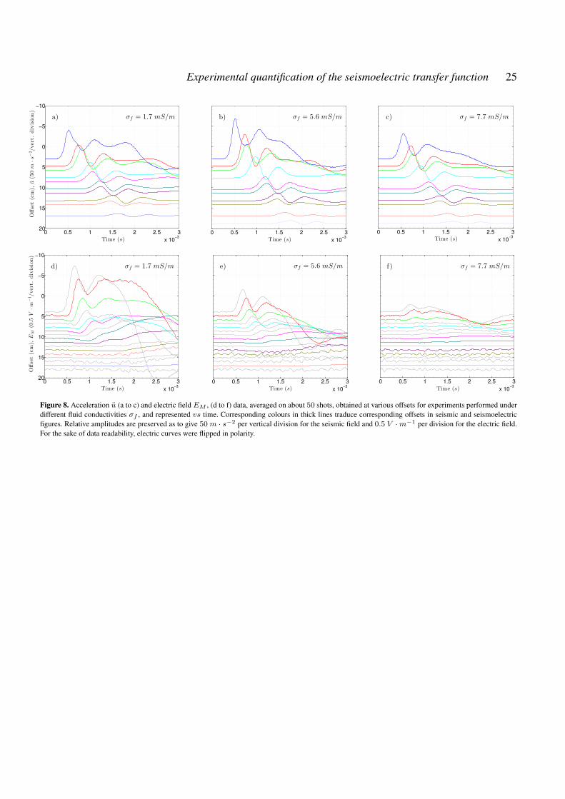
Experimental quantification of the seismoelectric transfer function 25
0 0.5 1 1.5 2 2.5 3
x 10−3
−10
−5
0
5
10
15
20
Offset(cm),
u(50m
·s−
2/vert.
division)
Time (s)
σf = 1.7 mS/ma)
0 0.5 1 1.5 2 2.5 3
x 10−3
Time (s)
σf = 5.6 mS/mb)
0 0.5 1 1.5 2 2.5 3
x 10−3Time (s)
σf = 7.7 mS/mc)
0 0.5 1 1.5 2 2.5 3
x 10−3
−10
−5
0
5
10
15
20
Offset(cm),
EM
(0.5
V·m
−1/vert.
division)
Time (s)
σf = 1.7 mS/md)
0 0.5 1 1.5 2 2.5 3
x 10−3Time (s)
σf = 5.6 mS/me)
0 0.5 1 1.5 2 2.5 3
x 10−3
Time (s)
σf = 7.7 mS/mf )
Figure 8. Acceleration u (a to c) and electric field EM , (d to f) data, averaged on about 50 shots, obtained at various offsets for experiments performed underdifferent fluid conductivities σf , and represented vs time. Corresponding colours in thick lines traduce corresponding offsets in seismic and seismoelectricfigures. Relative amplitudes are preserved as to give 50 m · s−2 per vertical division for the seismic field and 0.5 V ·m−1 per division for the electric field.For the sake of data readability, electric curves were flipped in polarity.
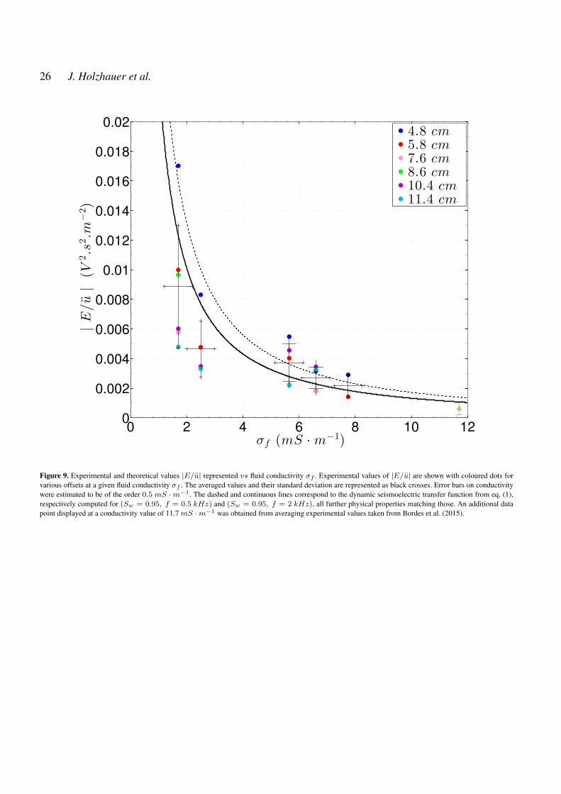
26 J. Holzhauer et al.
0 2 4 6 8 10 120
0.002
0.004
0.006
0.008
0.01
0.012
0.014
0.016
0.018
0.02
σf (mS · m−1)
|E/u|(V
2.s
2.m
−2)
4.8 cm5.8 cm7.6 cm8.6 cm10.4 cm11.4 cm
Figure 9. Experimental and theoretical values |E/u| represented vs fluid conductivity σf . Experimental values of |E/u| are shown with coloured dots forvarious offsets at a given fluid conductivity σf . The averaged values and their standard deviation are represented as black crosses. Error bars on conductivitywere estimated to be of the order 0.5 mS ·m−1. The dashed and continuous lines correspond to the dynamic seismoelectric transfer function from eq. (1),respectively computed for (Sw = 0.95, f = 0.5 kHz) and (Sw = 0.95, f = 2 kHz), all further physical properties matching those. An additional datapoint displayed at a conductivity value of 11.7 mS ·m−1 was obtained from averaging experimental values taken from Bordes et al. (2015).

Experimental quantification of the seismoelectric transfer function 27
0 0.2 0.4 0.6 0.8 110
2
103
Sw
VP(m
/s)
First imbibitionDrainageSecond imbibitionKf = KR
Kf = KB 61
Kf = KB 9
Kf = KB 32
Figure 10. P -wave velocities VP deduced from time-picking of the first seismic arrival during time-lapse monitored experiments with varying saturation Sw .The measurements were performed during initial imbibition, subsequent drainage and following re-imbibition. Velocity time-picking was performed betweenoffsets 10 to 23 cm. Error bars in velocity amplitudes were calculated from a linear regression of the time-picking vs offsets on a 80% confidence interval.The velocity models are represented by solid and dashed lines matching the colour of the corresponding experimental points. They were jointly obtainedby least-square inversion on these VP data and on the E/u data from Fig. 12, while adapting the effective fluid modulus Kf . All the velocity models arecomputed at a frequency f = 1.5 kHz.

28 J. Holzhauer et al.
−1 −0.5 0 0.5 1 1.5 2
x 10−3
0.2
0.4
0.6
0.8
1
Time (s)
Sw
Offset 3.9 cm
a)
−1 −0.5 0 0.5 1 1.5 2
x 10−3
0.2
0.4
0.6
0.8
1
Time (s)
Sw
Offset 5.8 cm
b)
Figure 11. Evolution of seismic (blue) and electric (red) signals vs time as a function of changes in water saturation Sw , for a set of experimental data acquiredduring drainage. Note that while water saturation is determined by the origin ordinate of each seismic curve, the vertical divisions on this same axis enableto get back to the signals amplitudes. The scale is of 10 m · s−2 per vertical division for the seismic field, and 0.025 V ·m−1 per vertical division for theelectric field. The origin on the time axis coincides with the initial punch of the pneumatic source. Seismic signals were taken for the first and second receiversat respective offsets a) 4.8 cm and b) 5.8 cm; electric signals were was taken for the mid-point dipole of length 1.8 cm placed at offset a) 3.9 cm and b)5.8 cm. Seismic signals in blue result from a stack 25. Electric signals in bold, dashed and light lines result respectively from stacks 50, 25 and 5.

Experimental quantification of the seismoelectric transfer function 29
0.4 0.6 0.8 1−5
−4
−3
−2
−1
0
1
2
3x 10
−3
Sw
E/u(V
·s2·m
−2)
First imbibitionDrainageSecond imbibitionKf = KR
Kf = KB 61
Kf = KB 9
Kf = KB 32
Figure 12. Experimental values of local E/u ratio estimated during time-lapse monitored experiments with varying saturation Sw . The measurements -performed during initial imbibition, subsequent drainage and following re-imbibition - are represented for a fluid conductivity of 7.2mS ·m−1. We consideredelectric data acquired at offset 3.9 cm, combined to seismic amplitudes extrapolated to a corresponding offset. Systematic error bars on the amplitude of E/uare of the order of 1 V · s2 · m−2 based on the uncertainties in electric and seismic pickings. The horizontal error bars on saturation are computed fromthe difference between the minimum and maximum values of the recorded saturation by the capacitance probes. The estimates of the transfer function arerepresented by solid and dashed lines matching the colour of the corresponding experimental points. They were jointly obtained by least-square inversion onthese E/u ratios and on the associated VP data from Fig. 10, while adapting the effective fluid modulus Kf . Models based on an effective fluid modulus ofthe Brie type with exponent e are notedKB e, whileKR points at an effective fluid modulus based on the Reuss average. Since the dynamic transfer functionseq. (1) is complex, the theoretical functions in the present figure are drawn as sign(real(E/u))× | E/u |. All model predictions are computed at a frequencyf = 1.5 kHz.
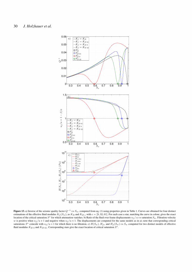
30 J. Holzhauer et al.
0.3 0.4 0.5 0.6 0.7 0.8 0.9 10
0.01
0.02
0.03
0.04
0.05
0.06
Sw
Q−1
Kf = KR
Kf = KB 61
Kf = KB 9
Kf = KB 32
S∗
R
S∗
B 61S∗
B 9S∗
B 32
a)
0.3 0.4 0.5 0.6 0.7 0.8 0.9 10.5
1
1.5
Sw
uf/u=
1−
β/φ
Kf = KR
Kf = KB 61
Kf = KB 9
Kf = KB 32
S∗
RS∗
B 61S∗
B 9S∗
B 32
b)
0.3 0.4 0.5 0.6 0.7 0.8 0.9 110
5
106
107
108
109
1010
X: 0.56
Y: 9e+07
Sw
H(S
w),H
fr,H
f(S
w)(P
a)
HB61HB9Hf rB61
HfB61
Hf rB9
HfB9
S∗
B61S∗
B9
c)
Figure 13. a) Inverse of the seismic quality factor Q−1 vs Sw , computed from eq. (1) using properties given in Table 1. Curves are obtained for four distinctestimations of the effective fluid modulus Kf (Sw), as KR and KB e with e = [9, 32, 61]. For each case a star, matching the curve in colour, gives the exactlocation of the critical saturation S∗ for which attenuation vanishes. b) Ratio of the fluid over frame displacements uf/ u vs saturation Sw . Filtration velocityw is positive when uf/u > 1 and negative when uf/u < 1. The displacements are computed for the same models as in a); note that corresponding criticalsaturations S∗ coincide with uf/u = 1 for which there is no filtration. c) H(Sw), Hfr and Hf (Sw) vs Sw computed for two distinct models of effectivefluid modulus KB 9 and KB 61. Corresponding stars give the exact location of critical saturation S∗.

Experimental quantification of the seismoelectric transfer function 31
LIST OF TABLES
1 Properties of the experimental porous medium constituted of Landes sand saturated by a water-gas fluid mixture. The listedparameters are divided into four main classes of properties concerning the fluid, the grain, the frame and the fluid-solid interface.They all intervene within the model computation of the coseismic seismoelectric phenomena presented in eq. (1), a model originallydescribed in Pride & Haartsen (1996), before being extended to partial saturation in Warden et al. (2013) and Bordes et al. (2015).Note that the electrolyte used in this Table is aNaCl solution: for that mixture we used the following relation between conductivityσf and concentration C0 (Haartsen & Pride (1997)): σf (C0) = e2 (bNa +bCl)C0NA×1000 ' C0×9.3 where e = 1.6×10⁻¹⁹
C is the elementary electric charge, bNa = bCl = 3 × 10¹¹ m · s−1 · N−1 are the ionic mobilities of cations and anions andNA = 6.022× 10²³mol−1 is the Avogadro number. The expression of L(Sw, ω) corresponds to a simplified expression given inBordes et al. (2015) where ωc(Sw) = 2πfBiot(Sw), where fBiot(Sw) is the critical pulsation defined upon the properties of theeffective fluid.

32 J. Holzhauer et al.
Parameter Notation and units Values Comments
Fluid Water density ρw (kg.m−3) 998 reference water valueWater viscosity ηw (Pa.s) 9.91× 10⁻⁴ Phillips et al. (1978)
Water permittivity εw 80 reference water valueWater modulus Kw (Pa) 2.2× 10⁹ reference water valueConductivity σf (mS.m−1) [1.7 − 10] measuredAir density ρg (kg.m−3) 1.2 reference air value
Air viscosity ηg (Pa.s) 1.8× 10⁻⁵ reference air valueAir modulus Kg (Pa) 1.5× 10⁵ reference air value
Effective Water saturation Sw [0.25 − 1] measuredfluid Residual saturation Sw0 0.25 measured
Fluid density ρf (kg.m−3) ρf (Sw) =ρg(1− Sw) + ρwSw −
Fluid viscosity ηf (Pa.s) ηf (Sw) =
ηg
(ηw
ηg
)Sw
Teja & Rice (1981)
Grain Solid density ρS (kg.m−3) 2650 reference silica valueGrain modulus KS (Pa) 3.6× 10¹⁰ reference silica value
Frame Porosity φ 0.42± 0.02 measuredPermeability k0 (m2) 2× 10⁻¹¹ measured
Tortuosity γ0 1.65± 0.15 Holzhauer (2015)Bulk modulus KD (Pa) 2.55× 10⁷ Barrière (2011) from Walton (1987)
5× 10⁷ (for drainage and second imbibition)Shear modulus G (Pa) 1.53× 10⁷ Barrière (2011) from Walton (1987)
3× 10⁷ (for drainage and second imbibition)Pore geometry factor mP 6 Pride (1994)2nd Archie param. n 2.58 Doussan & Ruy (2009); Bordes et al. (2015)
Fluid-solid Zeta potential ζ (mV ) 0.044 + 0.026 log[C0] adapted from Pride & Morgan (1991)interface
Electrokinetic coef.saturated
Cek(Sw = 1) =ε0εwζ
ηfσf
Cek (V · Pa−1) 7.14× 10⁻⁷ ζ(σf )
σfBordes et al. (2015)
Electrokinetic coef.Cek(Sw) =
Cek(Sw = 1)× f(Sw)− f(Sw) =
Sw − Sw0
1− Sw0S−nw from Jackson (2010)
Bordes et al. (2015)
Static SE coupling coef. L0(Sw) L0(Sw) = from Bordes et al. (2015)
(m2 · s−1 · V −1) −φ
γ0σfS
nwCek(Sw)
Dynamic SE coupling coef. L(Sw, ω) L (Sw, ω) = L0(Sw)× from Bordes et al. (2015)
(m2 · s−1 · V −1)
[1− i
ω
ωc(Sw)
mP
4
]−1/2
Table 1. Properties of the experimental porous medium constituted of Landes sand saturated by a water-gas fluid mixture. The listed parameters are dividedinto four main classes of properties concerning the fluid, the grain, the frame and the fluid-solid interface. They all intervene within the model computationof the coseismic seismoelectric phenomena presented in eq. (1), a model originally described in Pride & Haartsen (1996), before being extended to partialsaturation in Warden et al. (2013) and Bordes et al. (2015). Note that the electrolyte used in this Table is a NaCl solution: for that mixture we used thefollowing relation between conductivity σf and concentration C0 (Haartsen & Pride (1997)): σf (C0) = e2 (bNa + bCl)C0NA × 1000 ' C0 × 9.3where e = 1.6 × 10⁻¹⁹ C is the elementary electric charge, bNa = bCl = 3 × 10¹¹ m · s−1 · N−1 are the ionic mobilities of cations and anions andNA = 6.022× 10²³mol−1 is the Avogadro number. The expression of L(Sw, ω) corresponds to a simplified expression given in Bordes et al. (2015) whereωc(Sw) = 2πfBiot(Sw), where fBiot(Sw) is the critical pulsation defined upon the properties of the effective fluid.