experimental quantum computation with nuclear …luciano.stanford.edu/thesis/vandersypen.pdf ·...
TRANSCRIPT
EXPERIMENTAL QUANTUM COMPUTATION WITH
NUCLEAR SPINS IN LIQUID SOLUTION
a dissertation
submitted to the department of electrical engineering
and the committee on graduate studies
of stanford university
in partial fulfillment of the requirements
for the degree of
doctor of philosophy
Lieven M. K. Vandersypen
July 2001

ii

c© Copyright by Lieven M. K. Vandersypen 2001
All Rights Reserved
iii

iv

I certify that I have read this dissertation and that in my
opinion it is fully adequate, in scope and quality, as a disser-
tation for the degree of Doctor of Philosophy.
James S. Harris(Principal adviser)
I certify that I have read this dissertation and that in my
opinion it is fully adequate, in scope and quality, as a disser-
tation for the degree of Doctor of Philosophy.
Isaac L. Chuang(Co-adviser)
I certify that I have read this dissertation and that in my
opinion it is fully adequate, in scope and quality, as a disser-
tation for the degree of Doctor of Philosophy.
Yoshihisa Yamamoto
Approved for the University Committee on Graduate Studies:
v

vi

Abstract
Quantum computation offers the extraordinary promise of solving mathematical and phys-
ical problems which are simply beyond the reach of classical computers. However, the
experimental realization of quantum computers is extremely challenging, because of the
need to initialize, manipulate and measure the state of a set of coupled quantum systems
while maintaining fragile quantum coherence.
In this thesis work, we have taken significant steps towards the realization of a prac-
tical quantum computer: using nuclear spins and magnetic resonance techniques at room
temperature, we provided proof of principle of quantum computing in a series of experi-
ments which culminated in the implementation of the simplest instance of Shor’s quantum
algorithm for prime factorization (15 = 3 × 5), using a seven-spin molecule. This algo-
rithm achieves an exponential advantage over the best known classical factoring algorithms
and its implementation represents a milestone in the experimental exploration of quantum
computation.
These remarkable successes have been made possible by the synthesis of suitable molecules
and the development of many novel techniques for initialization, coherent control and read-
out of the state of multiple coupled nuclear spins. Furthermore, we devised and implemented
a model to simulate both unitary and decoherence processes in these systems, in order to
study and quantify the impact of various technological as well as fundamental sources of
errors.
In summary, this work has given us a much needed practical appreciation of what it
takes to build a quantum computer. Furthermore, while liquid NMR quantum computing
has well-understood scaling limitations, many of the techniques that originated from this
research may find use in other, perhaps more scalable quantum computer implementations.
vii

Preface
A long, long time ago, in a land far away, a man was sentenced to death. The man requested
to speak to the King, and the King agreed to hear him. “If you let me live for one more
year,” offered the man, “I promise to make your horse fly high above the land.” The
King realized that a flying horse would be quite unique, and took immense pleasure in the
prospect of possesing the only flying horse in the land. He agreed to set the man free and
let him live one more year.
When the man came home and told his wife what he had promised the King, she
exclaimed in anguish: “But you’ll never be able to make the King’s horse fly!”. “Well,”
said the man, “I know that, and you know that, but in the meantime many things can
happen. The country may go to war, the King may die, or the King’s horse may die, but I
will still be alive for another year.” 1
Now, can we build a quantum computer ? And should we promise to build one ? These
are the broad and ambitious questions underlying this thesis work. The final verdict is not1Free after James Harris. Thanks to for Nico for the drawing of the flying horse.
viii

in yet, and fortunately we are given more than one year. However, it is for certain that
only by studying quantum computation experimentally, can we begin to understand and
appreciate at a practical level what it would take to turn the dream of quantum computation
into reality. This is the purpose of my work.
ix
Acknowledgements
As a mechanical engineering sophomore at the Katholieke Universiteit Leuven, I took a great
and inspiring class in quantum mechanics with Guido Langouche. It was the beginning of
a profound interest in quantum mechanics, and a fascination which continues to this day.
Later, a second interest developed: to build mechanical systems on a very small scale. Two
other great courses, with Hendrik Van Brussel and Willy Sansen, gave me the opportunity
to further explore this area.
When I came to Stanford University for graduate school, I was looking for a project
to combine these two interests, for example by studying if and how quantum mechani-
cal effects could be observed in micromachined structures. For one quarter, I worked on
microcantilevers in the most stimulating group of Yoshihisa Yamamoto.
Then I talked to Jim Harris, who suggested I try to microfabricate components for an
NMR quantum computer. Soon after I talked Ike Chuang, the initiator of this project (then
at Los Alamos, later at IBM Almaden), and started reading about quantum computing, I
became increasingly fascinated by quantum computing itself. I knew this is what I wanted
to work on!
It was the beginning of an extraordinary four years, four years I am very thankful for.
The fact that this has been such a wonderful time is due to many great people.
Jim Harris, my advisor and “coach”, has generously introduced me to the right people to
make my work a success, and strongly supported me in many ways, in and outside research.
His view on life and on what is really important is a true inspiration to me. Ike Chuang,
my co-advisor, gave me both guidance and independence, at the right times. He taught me
how to present my work and put it in perspective, and also to think positive and creatively
(to say “what would it take to make this work” instead of “this won’t work”). Also, Coach’s
and Ike’s strong support and belief in my abilities, as well as their encouragement for my
non-research activities, have been invaluable to me.
x

Matthias Steffen worked very closely with me for about two years and a half, first as an
apprentice, but increasingly as a great co-worker. He brought in many useful ideas and did
a lot of the work in the later experiments. Xinlan Zhou kindly helped me out with many
theoretical questions throughout the past years.
Nino Yannoni discovered most of the molecules we have used, and also provided me with
many wise words. Mark Sherwood has greatly contributed for concepts and techniques in
NMR and for molecule selection. Greg Breyta gave us a lot of the time he didn’t have, to
synthesize the five and seven spin molecules.
I am very grateful to my other co-authors, in particular Richard Cleve, with whom I
worked so pleasantly. I am also indepted to the many colleagues from whom I’ve learnt and
with whom I had such nice interactions (especially Dorit Aharonov, Michael Nielsen, David
DiVincenzo and Ray Freeman).
My close colleagues Anne Verhulst and Oskar Liivak have contributed to a great working
environment and provided many useful discussions. So have the many summer students in
the group.
Lois Durham made her NMR lab available for my early experiments, and we have had
a fruitful collaboration with the people at Varian NMR.
At Stanford, I have particularly enjoyed Tom Cover’s lectures on information theory.
He gave me a deep apprecation for this beautiful field, which is now being revisited in the
context of quantum information. Similarly, Rajeev Motwani’s course on classical complexity
theory and automata helped me put quantum computation in perspective.
Patricia Ryan, coach of the Stanford Improvisors, has affected my life in a very positive
way. I say “yes” more often now, I have more adventures, and I learnt it’s ok if things
don’t always work out. Philip Zimbardo’s course on psychology has been an inspiration for
teaching and a lesson for life.
The financial support of a Francqui Fellowship of the Belgian-American Educational
Foundation, a Yansouni Family Stanford Graduate Fellowship, DARPA, and IBM Research,
have given me the opportunity to freely pursue my interests.
The warm support of my parents, family, friends (especially PS, EV and PC) and
roommates has done me much good, especially in the days when things didn’t go so well. I
cherish the many good moments I shared with all of them.
xi
Contents
Abstract vii
Preface viii
Acknowledgements x
1 Introduction 1
1.1 Historical background . . . . . . . . . . . . . . . . . . . . . . . . . . . . . . 1
1.2 Purpose of my work . . . . . . . . . . . . . . . . . . . . . . . . . . . . . . . 4
1.3 Organization of the dissertation . . . . . . . . . . . . . . . . . . . . . . . . . 5
1.4 Literature . . . . . . . . . . . . . . . . . . . . . . . . . . . . . . . . . . . . . 6
2 Theory of quantum computation 9
2.1 Fundamental concepts . . . . . . . . . . . . . . . . . . . . . . . . . . . . . . 9
2.1.1 Quantum bits . . . . . . . . . . . . . . . . . . . . . . . . . . . . . . . 9
2.1.2 Computation using quantum systems . . . . . . . . . . . . . . . . . . 14
2.1.3 Quantum parallellism . . . . . . . . . . . . . . . . . . . . . . . . . . 17
2.1.4 Quantum algorithms . . . . . . . . . . . . . . . . . . . . . . . . . . . 22
2.1.5 Correcting quantum errors . . . . . . . . . . . . . . . . . . . . . . . 24
2.2 Quantum gates and circuits . . . . . . . . . . . . . . . . . . . . . . . . . . . 26
2.2.1 Directly implementable quantum gates . . . . . . . . . . . . . . . . . 27
2.2.2 Universality . . . . . . . . . . . . . . . . . . . . . . . . . . . . . . . . 31
2.2.3 Remarks on unitary operators . . . . . . . . . . . . . . . . . . . . . . 32
2.2.4 Multi-qubit gates . . . . . . . . . . . . . . . . . . . . . . . . . . . . . 34
2.3 Quantum algorithms . . . . . . . . . . . . . . . . . . . . . . . . . . . . . . . 35
2.3.1 The Deutsch-Jozsa algorithm . . . . . . . . . . . . . . . . . . . . . . 35
xii
2.3.2 Grover’s algorithm . . . . . . . . . . . . . . . . . . . . . . . . . . . . 39
2.3.3 Order-finding and Shor’s algorithm . . . . . . . . . . . . . . . . . . . 42
2.3.4 Quantum simulations . . . . . . . . . . . . . . . . . . . . . . . . . . 50
2.3.5 Other quantum algorithms and perspectives . . . . . . . . . . . . . . 51
2.4 Quantum error correction . . . . . . . . . . . . . . . . . . . . . . . . . . . . 52
2.4.1 The two-qubit phase error detection code . . . . . . . . . . . . . . . 53
2.4.2 Error correction codes and fault-tolerancy . . . . . . . . . . . . . . . 56
2.5 Summary . . . . . . . . . . . . . . . . . . . . . . . . . . . . . . . . . . . . . 57
3 Implementation of quantum computers 58
3.1 Requirements . . . . . . . . . . . . . . . . . . . . . . . . . . . . . . . . . . . 58
3.1.1 Qubits . . . . . . . . . . . . . . . . . . . . . . . . . . . . . . . . . . . 59
3.1.2 Quantum gates . . . . . . . . . . . . . . . . . . . . . . . . . . . . . . 60
3.1.3 Initialization . . . . . . . . . . . . . . . . . . . . . . . . . . . . . . . 65
3.1.4 Read-out . . . . . . . . . . . . . . . . . . . . . . . . . . . . . . . . . 68
3.1.5 Coherence . . . . . . . . . . . . . . . . . . . . . . . . . . . . . . . . . 71
3.2 State of the art . . . . . . . . . . . . . . . . . . . . . . . . . . . . . . . . . . 77
3.2.1 Trapped ions . . . . . . . . . . . . . . . . . . . . . . . . . . . . . . . 77
3.2.2 Neutral atoms . . . . . . . . . . . . . . . . . . . . . . . . . . . . . . 79
3.2.3 Quantum dots . . . . . . . . . . . . . . . . . . . . . . . . . . . . . . 82
3.2.4 Superconducting qubits . . . . . . . . . . . . . . . . . . . . . . . . . 85
3.2.5 Solid-state NMR . . . . . . . . . . . . . . . . . . . . . . . . . . . . . 87
3.2.6 Dopants in semiconductors . . . . . . . . . . . . . . . . . . . . . . . 90
3.2.7 Other proposals . . . . . . . . . . . . . . . . . . . . . . . . . . . . . . 93
3.3 Summary . . . . . . . . . . . . . . . . . . . . . . . . . . . . . . . . . . . . . 93
4 Liquid-state NMR quantum computing 95
4.1 Qubits . . . . . . . . . . . . . . . . . . . . . . . . . . . . . . . . . . . . . . . 95
4.1.1 Single-spin Hamiltonian . . . . . . . . . . . . . . . . . . . . . . . . . 96
4.1.2 Spin-spin interaction Hamiltonian . . . . . . . . . . . . . . . . . . . 97
4.2 Single-qubit operations . . . . . . . . . . . . . . . . . . . . . . . . . . . . . . 100
4.2.1 Rotations about an axis in the xy plane (RF pulses) . . . . . . . . . 100
4.2.2 Rotations about the z axis . . . . . . . . . . . . . . . . . . . . . . . 103
4.2.3 Selective excitation using pulse shaping . . . . . . . . . . . . . . . . 104
xiii
4.2.4 Single pulses - artefacts and solutions . . . . . . . . . . . . . . . . . 107
4.2.5 Simultaneous pulses - artefacts and solutions . . . . . . . . . . . . . 110
4.3 Two-qubit operations . . . . . . . . . . . . . . . . . . . . . . . . . . . . . . 114
4.3.1 The controlled-not in a two-spin system . . . . . . . . . . . . . . . . 114
4.3.2 Refocusing select J couplings . . . . . . . . . . . . . . . . . . . . . . 116
4.4 Qubit initialization . . . . . . . . . . . . . . . . . . . . . . . . . . . . . . . . 120
4.4.1 The initial state of nuclear spins . . . . . . . . . . . . . . . . . . . . 120
4.4.2 Effective pure states . . . . . . . . . . . . . . . . . . . . . . . . . . . 122
4.4.3 Logical labeling . . . . . . . . . . . . . . . . . . . . . . . . . . . . . . 124
4.4.4 Temporal averaging . . . . . . . . . . . . . . . . . . . . . . . . . . . 126
4.4.5 Spatial averaging . . . . . . . . . . . . . . . . . . . . . . . . . . . . . 130
4.4.6 Efficient cooling . . . . . . . . . . . . . . . . . . . . . . . . . . . . . 131
4.5 Read-out . . . . . . . . . . . . . . . . . . . . . . . . . . . . . . . . . . . . . 133
4.5.1 NMR spectra . . . . . . . . . . . . . . . . . . . . . . . . . . . . . . . 133
4.5.2 Quantum state tomography . . . . . . . . . . . . . . . . . . . . . . . 137
4.6 Decoherence . . . . . . . . . . . . . . . . . . . . . . . . . . . . . . . . . . . . 138
4.6.1 Principal mechanisms . . . . . . . . . . . . . . . . . . . . . . . . . . 138
4.6.2 Characterization . . . . . . . . . . . . . . . . . . . . . . . . . . . . . 141
4.7 Molecule design . . . . . . . . . . . . . . . . . . . . . . . . . . . . . . . . . . 143
4.8 Pulse sequence design . . . . . . . . . . . . . . . . . . . . . . . . . . . . . . 144
4.8.1 Simplification at three levels . . . . . . . . . . . . . . . . . . . . . . 145
4.8.2 Design for robustness . . . . . . . . . . . . . . . . . . . . . . . . . . 148
4.9 Summary . . . . . . . . . . . . . . . . . . . . . . . . . . . . . . . . . . . . . 148
5 Experimental realization of NMR quantum computers 150
5.1 Experimental apparatus . . . . . . . . . . . . . . . . . . . . . . . . . . . . . 150
5.1.1 Sample . . . . . . . . . . . . . . . . . . . . . . . . . . . . . . . . . . 151
5.1.2 Magnet . . . . . . . . . . . . . . . . . . . . . . . . . . . . . . . . . . 152
5.1.3 Probe . . . . . . . . . . . . . . . . . . . . . . . . . . . . . . . . . . . 155
5.1.4 Transmitter . . . . . . . . . . . . . . . . . . . . . . . . . . . . . . . . 158
5.1.5 Receiver . . . . . . . . . . . . . . . . . . . . . . . . . . . . . . . . . . 160
5.1.6 Workstation . . . . . . . . . . . . . . . . . . . . . . . . . . . . . . . . 161
5.2 Overview of NMR quantum computing experiments . . . . . . . . . . . . . 163
xiv
5.3 A first quantum algorithm (2 spins) . . . . . . . . . . . . . . . . . . . . . . 166
5.3.1 Problem description . . . . . . . . . . . . . . . . . . . . . . . . . . . 166
5.3.2 Experimental procedure . . . . . . . . . . . . . . . . . . . . . . . . . 168
5.3.3 Experimental results . . . . . . . . . . . . . . . . . . . . . . . . . . . 169
5.3.4 Discussion . . . . . . . . . . . . . . . . . . . . . . . . . . . . . . . . . 169
5.4 Quantum error detection (2 spins) . . . . . . . . . . . . . . . . . . . . . . . 172
5.4.1 Problem description . . . . . . . . . . . . . . . . . . . . . . . . . . . 172
5.4.2 Experimental procedure . . . . . . . . . . . . . . . . . . . . . . . . . 172
5.4.3 Experimental results . . . . . . . . . . . . . . . . . . . . . . . . . . . 174
5.4.4 Discussion . . . . . . . . . . . . . . . . . . . . . . . . . . . . . . . . . 175
5.5 Logical labeling (3 spins) . . . . . . . . . . . . . . . . . . . . . . . . . . . . 177
5.5.1 Problem description . . . . . . . . . . . . . . . . . . . . . . . . . . . 177
5.5.2 Experimental procedure . . . . . . . . . . . . . . . . . . . . . . . . . 178
5.5.3 Experimental results . . . . . . . . . . . . . . . . . . . . . . . . . . . 180
5.5.4 Discussion . . . . . . . . . . . . . . . . . . . . . . . . . . . . . . . . . 182
5.6 Liquid crystal solutions (2 spins) . . . . . . . . . . . . . . . . . . . . . . . . 183
5.6.1 Problem description . . . . . . . . . . . . . . . . . . . . . . . . . . . 183
5.6.2 Experimental approach and results . . . . . . . . . . . . . . . . . . . 185
5.6.3 Discussion . . . . . . . . . . . . . . . . . . . . . . . . . . . . . . . . . 187
5.7 Cancellation and prevention of systematic errors (3 spins) . . . . . . . . . . 188
5.7.1 Problem description . . . . . . . . . . . . . . . . . . . . . . . . . . . 188
5.7.2 Experimental approach . . . . . . . . . . . . . . . . . . . . . . . . . 189
5.7.3 Experimental Results . . . . . . . . . . . . . . . . . . . . . . . . . . 190
5.7.4 Discussion . . . . . . . . . . . . . . . . . . . . . . . . . . . . . . . . . 191
5.8 Efficient cooling (3 spins) . . . . . . . . . . . . . . . . . . . . . . . . . . . . 192
5.8.1 Problem description . . . . . . . . . . . . . . . . . . . . . . . . . . . 192
5.8.2 Experimental procedure and results . . . . . . . . . . . . . . . . . . 193
5.8.3 Experimental results . . . . . . . . . . . . . . . . . . . . . . . . . . . 196
5.8.4 Discussion . . . . . . . . . . . . . . . . . . . . . . . . . . . . . . . . . 197
5.9 Order-finding (5 spins) . . . . . . . . . . . . . . . . . . . . . . . . . . . . . . 198
5.9.1 Problem description . . . . . . . . . . . . . . . . . . . . . . . . . . . 198
5.9.2 Experimental approach . . . . . . . . . . . . . . . . . . . . . . . . . 199
5.9.3 Experimental results . . . . . . . . . . . . . . . . . . . . . . . . . . . 202
xv

5.9.4 Discussion . . . . . . . . . . . . . . . . . . . . . . . . . . . . . . . . . 202
5.10 Shor’s factoring algorithm (7 spins) . . . . . . . . . . . . . . . . . . . . . . . 203
5.10.1 Problem description . . . . . . . . . . . . . . . . . . . . . . . . . . . 203
5.10.2 Experimental approach . . . . . . . . . . . . . . . . . . . . . . . . . 207
5.10.3 Experimental results . . . . . . . . . . . . . . . . . . . . . . . . . . . 212
5.10.4 Decoherence model . . . . . . . . . . . . . . . . . . . . . . . . . . . . 215
5.10.5 Discussion . . . . . . . . . . . . . . . . . . . . . . . . . . . . . . . . . 219
5.11 Summary . . . . . . . . . . . . . . . . . . . . . . . . . . . . . . . . . . . . . 219
6 Conclusions 222
A Numerical model 225
A.1 Set up the Hamiltonian and Pauli matrices . . . . . . . . . . . . . . . . . . 225
A.2 Action unitary operator on density matrix . . . . . . . . . . . . . . . . . . . 227
A.3 Time evolution under the Hamiltonian . . . . . . . . . . . . . . . . . . . . . 227
A.4 Single-spin rotations . . . . . . . . . . . . . . . . . . . . . . . . . . . . . . . 227
A.5 Generalized amplitude damping . . . . . . . . . . . . . . . . . . . . . . . . . 228
A.6 Phase damping . . . . . . . . . . . . . . . . . . . . . . . . . . . . . . . . . . 229
A.7 Helper programs . . . . . . . . . . . . . . . . . . . . . . . . . . . . . . . . . 231
A.8 Pulse sequence code in MATLAB . . . . . . . . . . . . . . . . . . . . . . . . 232
B Pulse sequence three-spin Grover search 233
Bibliography 236
xvi

List of Tables
4.1 Larmor frequencies [Mhz] of some relevant nuclei, at 11.74 Tesla. . . . . . . 97
4.2 Properties of relevant pulse shapes . . . . . . . . . . . . . . . . . . . . . . . 107
4.3 Comparison of the degree to which J-coupled evolution during a single pulse
on spin 1 is unwound via asymmetric versus symmetric negative time inter-
vals τ (expressed as a fraction of the duration of pw), for various coupling
scenarios. The optimal τ is indicated in each case. . . . . . . . . . . . . . . 110
4.4 Comparison of the degree to which J-coupled evolution during two pulses
is unwound for three scenario’s: (1) two pulses back to back preceeded and
followed by negative evolution, (2) two simultaneous pulses preceeded and
followed by negative evolution, and for comparison (3) two simultaneous
pulses only followed by negative evolution. The optimal τ is indicated in
each case. . . . . . . . . . . . . . . . . . . . . . . . . . . . . . . . . . . . . . 114
5.1 13C-1H spin couplings [Hz] and relaxation times [s] for 13C1HCl3 in isotropic
(deuterated acetone) and liquid crystal (ZLI-1167) solution. . . . . . . . . . 185
5.2 The table gives f(x) = axmod 15 for all a < 15 coprime with 15 and for
successive values of x. For each value of a, the period r emerges from the
sequence of output values f(x). Calculation of the greatest common denom-
inator of ar/2 ± 1 and 15 then gives at least one prime factor of 15. . . . . . 205
5.3 First stage of the temporal averaging procedure to prepare an effective pure
state of five nuclei of the same species and two other nuclei of another species.
The table shows how the terms in the thermal equilibrium density matrix are
transformed by each temporal averaging sequence (the IIIIIZI and IIIIIIZ
terms are not shown as they are left unaffected in this first stage). Cij stands
for cnotij and Ni stands for noti. . . . . . . . . . . . . . . . . . . . . . . . 209
xvii
List of Figures
1.1 Connections between the four main chapters of this thesis work. . . . . . . 6
2.1 (a) Bloch sphere representation of the state |ψ〉 of a single qubit. (b) The
position in the Bloch sphere of four important states. By convention, we will
always let |0〉 be along +z. . . . . . . . . . . . . . . . . . . . . . . . . . . . . 10
2.2 Truth table for (a) The traditional and gate; the output is 1 when both
inputs are 1, and the output is 0 otherwise. (b) The extended and gate,
with two output bits. (c) A reversible and gate, also known as the Toffoli
gate. . . . . . . . . . . . . . . . . . . . . . . . . . . . . . . . . . . . . . . . . 16
2.3 A message (one or more bits or qubits) is first redundantly encoded, the en-
coded message then goes through the process of interest (transmission over a
noisy channel, a computation subject to errors, etcetera), and finally the cor-
rupted encoded message is decoded and corrections are made if needed, based
on the error syndrome (information about which errors occurred, contained
in the redudancy bits. . . . . . . . . . . . . . . . . . . . . . . . . . . . . . . 26
2.4 The quantum circuit representation of (a) an arbitrary one-qubit gate U and
of (b) the not gate. . . . . . . . . . . . . . . . . . . . . . . . . . . . . . . . 30
2.5 Truth table of the cnot gate with (Left) the first qubit in the role of the
control qubit and (Right) the second qubit in the role of the control qubit. . 30
2.6 Quantum circuits for (a) the cnot12 gate, (b) the swap gate, (c) a controlled-
U gate and (d) a zero-controlled-U gate. The • symbol indicates the control
qubit; it controls the operation it is connected to via a vertical line. The
symbol indicates a zero-control qubit. A vertical line connecting two ×symbols denotes a swap operation of the two qubits. . . . . . . . . . . . . . 31
xviii

2.7 Quantum circuit representation of the Toffoli or ccnot gate, and its de-
composition into two-qubit gates. We note that V 2 = Unot. . . . . . . . . 35
2.8 Quantum circuit representation of the Fredkin or cswap gate, and two
quantum circuits equivalent to the Fredkin gate. . . . . . . . . . . . . . . 35
2.9 Quantum circuit for the Deutsch-Jozsa algorithm. . . . . . . . . . . . . . . 37
2.10 Illustration of amplitude amplification in Grover’s algorithm for N = 8 (n =
3) and |x0〉 = |101〉. The diagrams shows the (real) amplitude of the eight
terms |000〉 through |111〉. The starting point is an equal superposition of
all terms. After each Grover iteration (an oracle call followed by inversion
about the average), the amplitude of the special element is amplified. For
the case N = 8, the amplitude of the |x0〉 reaches almost 1 after two Grover
iterations. . . . . . . . . . . . . . . . . . . . . . . . . . . . . . . . . . . . . . 41
2.11 Quantum circuit for the quantum Fourier transform (QFT) acting on three
qubits. In this implementation of the QFT, due to Coppersmith [Cop94], the
order of the qubits is reversed at the output with respect to the input. . . . 45
2.12 Pictorial representation of a permutation π on eight elements. The order r
is 3 if y ∈ 2, 4, 5, r = 1 if y = 6, and r = 4 if y ∈ 0, 1, 3, 7. . . . . . . . . 45
2.13 Outline of the order-finding quantum algorithm. . . . . . . . . . . . . . . . 47
2.14 Encoding and decoding quantum circuit for the two-qubit code. In between
encoding and decoding, phase damping may disturb the qubit states. . . . . 54
3.1 Three extreme coupling networks between five qubits. (a) A full coupling
network. (b) A nearest-neighbour coupling network. (c) Coupling via a bus. 61
3.2 Schematic diagram (after [CZ95]) of an ion trap containing six ions (the
electrodes needed to keep the ions on one line are not shown). Each ion can
be individually addressed with laser pulses, and the collective vibrational
motion of the ions serves as a bus qubit. . . . . . . . . . . . . . . . . . . . . 77
3.3 Model energy level diagram of the relevant internal states in a trapped ion.
The qubit is embodied by |0〉 and |1〉. Level |1′〉 assists in two qubit operations
and level |s〉 is used during read-out. . . . . . . . . . . . . . . . . . . . . . . 78
3.4 A single two-level atom is trapped by the cavity mode of a single photon.
The cavity consists of two curved mirrors. (after Mabuchi in [MPZ00]) . . . 80
xix
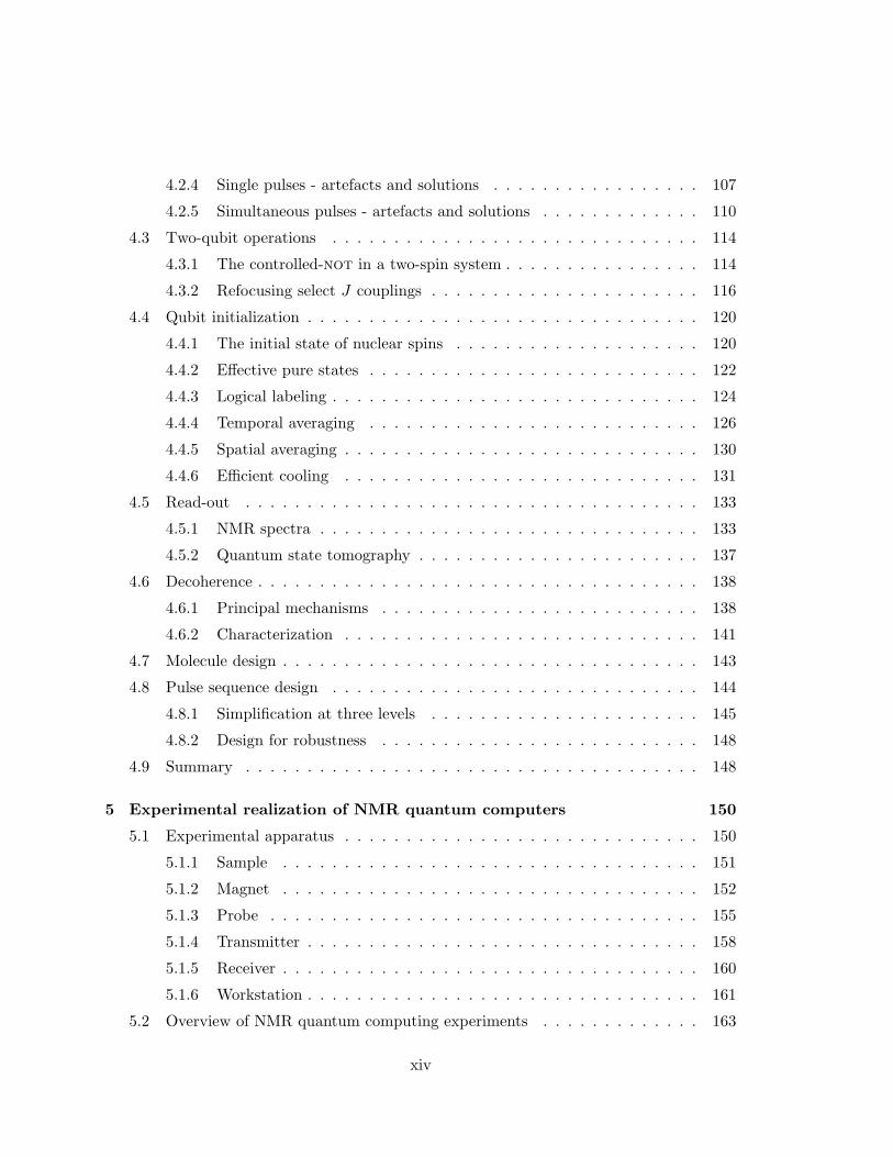
3.5 Conceptual schematic (after [DL99]) of one variant of a quantum dot quan-
tum computer. Lateral side gates on top of a two-dimensional electron gas
(created for example via a AlGaAs/GaAs/AlGaAs quantum well) confine the
motion of an electron to a very small area (the quantum dot). The tunnel-
ing barrier between neighbouring quantum dots can be controlled via the
voltages on the gates. . . . . . . . . . . . . . . . . . . . . . . . . . . . . . . 82
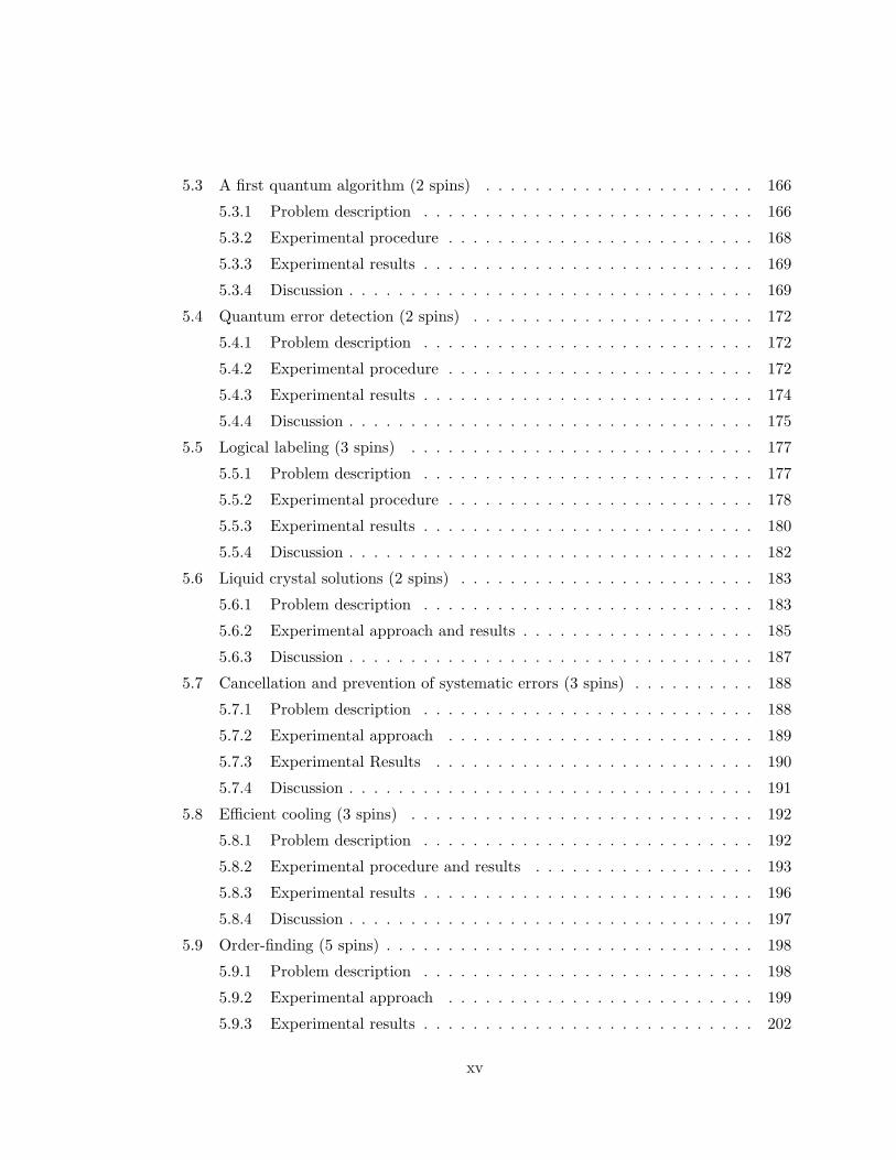
3.6 Schematic of two superconducting flux qubits, each embodied by a small su-
perconducting loop interrupted by Josephson junctions (small barriers made
of a resistive material). The devices shown contain three Josephson junctions,
as in [vtW+00]. . . . . . . . . . . . . . . . . . . . . . . . . . . . . . . . . . . 85
3.7 Schematic of a superconducting charge qubit, realized by a small supercon-
ducting island or “box”, coupled to the ground via a Josephson junction.
The electrostatic potential of the island is controlled by the gate voltage Vg.
The dashed part of the circuit serves for readout; it is not part of the actual
qubit. In practice, improved variations of this design are used, which use
more Josephson junctions in order to be able to have more control over the
qubit parameters. . . . . . . . . . . . . . . . . . . . . . . . . . . . . . . . . . 86
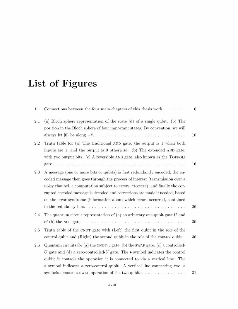
3.8 Model of a crystal lattice quantum computer. The crystal shown here has a
simple cubic lattice; in practice other lattices have been proposed, but the
idea is the same. The nuclei 1, 2, 3, . . . form one quantum computer, the
nuclei a, b, c, . . . form an independent computer, and so forth. Nuclei 1, a
and A represent the analogous qubit in the respective computers. . . . . . . 88
3.9 Model of a Kane-type quantum computer (cross-section), after [Kan98]. . . 90
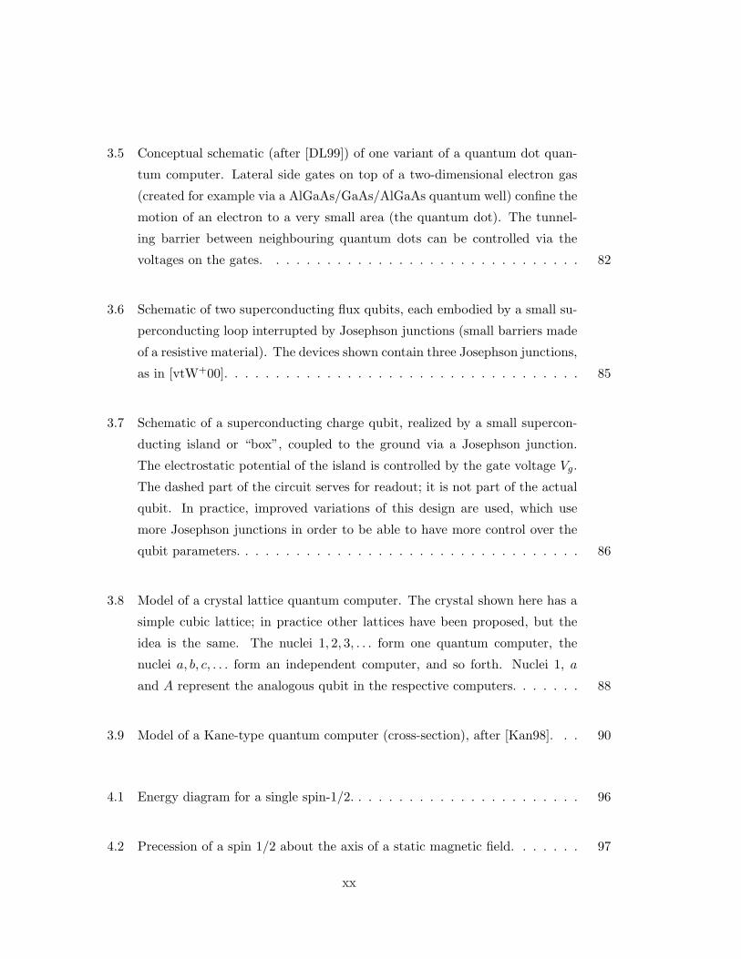
4.1 Energy diagram for a single spin-1/2. . . . . . . . . . . . . . . . . . . . . . . 96
4.2 Precession of a spin 1/2 about the axis of a static magnetic field. . . . . . . 97
xx
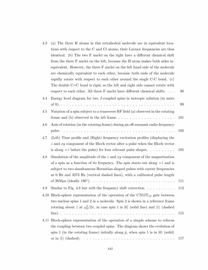
4.3 (a) The three H atoms in this tetrahedral molecule are in equivalent loca-
tions with respect to the C and Cl atoms; their Larmor frequencies are thus
identical. (b) The two F nuclei on the right have a different chemical shift
from the three F nuclei on the left, because the H atom makes both sides in-
equivalent. However, the three F nuclei on the left hand side of the molecule
are chemically equivalent to each other, because both ends of the molecule
rapidly rotate with respect to each other around the single C-C bond. (c)
The double C=C bond is rigid, so the left and right side cannot rotate with
respect to each other. All three F nuclei have different chemical shifts. . . . 98
4.4 Energy level diagram for two J-coupled spins in isotropic solution (in units
of ~). . . . . . . . . . . . . . . . . . . . . . . . . . . . . . . . . . . . . . . . . 99
4.5 Nutation of a spin subject to a transverse RF field (a) observed in the rotating
frame and (b) observed in the lab frame. . . . . . . . . . . . . . . . . . . . . 101
4.6 Axis of rotation (in the rotating frame) during an off-resonant radio-frequency
pulse. . . . . . . . . . . . . . . . . . . . . . . . . . . . . . . . . . . . . . . . 102
4.7 (Left) Time profile and (Right) frequency excitation profiles (displaying the
z and xy component of the Bloch vector after a pulse when the Bloch vector
is along +z before the pulse) for four relevant pulse shapes. . . . . . . . . . 105
4.8 Simulation of the amplitude of the z and xy component of the magnetization
of a spin as a function of its frequency. The spin starts out along +z and is
subject to two simultaneous Hermitian shaped pulses with carrier frequencies
at 0 Hz and 3273 Hz (vertical dashed lines), with a calibrated pulse length
of 2650µs (ideally 180). . . . . . . . . . . . . . . . . . . . . . . . . . . . . . 111
4.9 Similar to Fig. 4.8 but with the frequency shift correction. . . . . . . . . . . 112
4.10 Bloch-sphere representation of the operation of the CNOT12 gate between
two nuclear spins 1 and 2 in a molecule. Spin 2 is shown in a reference frame
rotating about z at ω20/2π, in case spin 1 is |0〉 (solid line) and |1〉 (dashed
line). . . . . . . . . . . . . . . . . . . . . . . . . . . . . . . . . . . . . . . . . 115
4.11 Bloch-sphere representation of the operation of a simple scheme to refocus
the coupling between two coupled spins. The diagram shows the evolution of
spin 1 (in the rotating frame) initially along y, when spin 1 is in |0〉 (solid)
or in |1〉 (dashed). . . . . . . . . . . . . . . . . . . . . . . . . . . . . . . . . 117
xxi

4.12 Refocusing scheme for a four spin system. J12 is active the whole time but
the effect of the other Jij is neutralized. The interval is divided into slices of
equal duration, and the “+” and “-” signs indicate whether a spin is still in
its original position, or upside down. At the interface of certain time slices,
180 pulses (assumed to be instantaneous, and shown as black retangles) are
sent on one or more spins; the pulsed spins transition from + to − or back. 118
4.13 Simplified refocusing scheme for five spins, which can be used if we know in
advance that spins 3, 4 and 5 are along ±z. J12 is active, but J13, J14, J15,
J23, J24, J25 are inactive. The remaining couplings are active but have no
effect given the initial state. . . . . . . . . . . . . . . . . . . . . . . . . . . . 118
4.14 A quantum circuit that implements the Schulman-Vazirani boosting proce-
dure. The controlled-swap (Fredkin) gate has been replaced by two cnot’s
and a Toffoli gate, as in Fig. 2.8. . . . . . . . . . . . . . . . . . . . . . . . 131
4.15 The thermal equilibrium spectrum (amplitude of the real part) of spin 1 in
a molecule of five coupled spins (more details on this molecule are given
in section 5.9). Frequencies are given in units of Hz, with respect to ω10.
The state of the remaining spins is as indicated, based on J12 < 0 and
J13, J14, J15 > 0; furthermore, |J12| > |J13| > |J15| > |J14|. . . . . . . . . . . 135
4.16 Simplification rules for quantum circuits . . . . . . . . . . . . . . . . . . . . 146
4.17 Commutation of unitary operators can help simplify quantum circuits by
moving building blocks around such that cancellations of operations as in
Fig. 4.16 become possible. For example, the three components (separated
by dashed lines) in these two equivalent realizations of the Toffoli gate
commute with each other and can thus be executed in any order. . . . . . . 146
4.18 Choosing one of several equivalent implementations can help simplify quan-
tum circuits, again by enabling cancellation of operations as in Fig. 4.16.
The Toffoli gate has two control qubits, whose role is symmetric and can
thus be swapped. . . . . . . . . . . . . . . . . . . . . . . . . . . . . . . . . . 147
5.1 Schematic overview of an NMR apparatus. . . . . . . . . . . . . . . . . . . . 151
5.2 A typical NMR sample. The sample tube is held by a sample holder when it
is inserted in the superconducting magnet. . . . . . . . . . . . . . . . . . . . 152
xxii

5.3 Oxford Instruments 500 MHz wide-bore NMR magnet. Fill ports for liquid
nitrogen and helium stick out from the top. The cabinet near one of the
magnet legs contains transmit/receive switches, preamplifiers and mixers.
The probe is inserted in the bore of the magnet from below and the sample
is inserted from the top. It sits in the probe in the center of the solenoid. . 153
5.4 Nalorac HFX Probe. The RF coils sit near the top of the probe. BNC
connectors, a cooling air inlet, a connector for the gradient coils and knobs
to adjust to tune/match capacitors are visible at the bottom of the probe. . 156
5.5 Spectrometer electronics cabinet. The magnet is visible behind the cabinet. 159
5.6 Overview of quantum computing experiments. The difficulty of an experi-
ment depends mainly on two parameters: (1) the number of qubits involved
and (2) the complexity of the protocol executed with those qubits, in terms
of the number of gates and the demands on the coupling network (e.g. exper-
iments using only nearest neighbour couplings are easier than experiments
which need a complete or nearly complete coupling network). Numbers next
to the data are the year published. . . . . . . . . . . . . . . . . . . . . . . . 167
5.7 Quantum circuit for performing the simplest instance of the Deutsch-Jozsa
algorithm. . . . . . . . . . . . . . . . . . . . . . . . . . . . . . . . . . . . . . 168
5.8 Proton spectrum after completion of the Deutsch-Jozsa algorithm and a sin-
gle read-out pulse X1, with an effectively pure input state |00〉 and with a
thermal input state [Inset]. The low (high) frequency lines correspond to the
transitions |00〉 ↔ |10〉 (|01〉 ↔ |11〉). The frequency is relative to ω10 (the
Larmor frequency of spin 1), and the amplitude has arbitrary units. The
phase is set such that a spectral line is real and positive (negative) when spin
1 is |0〉 (|1〉) right before the read-out pulse. . . . . . . . . . . . . . . . . . . 170
5.9 Experimentally measured and theoretically expected deviation density matri-
ces after completion of the Deutsch-Jozsa algorithm. The diagonal elements
represent the normalized populations of the states |00〉, |01〉, |10〉 and |11〉(from left to right). The off-diagonal elements represent coherences between
different states. The magnitudes are shown with the sign of the real compo-
nent; all imaginary components were small. . . . . . . . . . . . . . . . . . . 171
5.10 Schematic diagram for the two-bit code experiment. . . . . . . . . . . . . . 173
xxiii

5.11 Predicted Bloch spheres (a) with and (b) without encoding, for a set of
equally spaced storage times (k × 61.5 ms for k = 0, 1 . . . ,5), corresponding
to a probability of phase error (without encoding) of p = 0, 0.071, 0.133,
0.185, 0.230 and 0.269. . . . . . . . . . . . . . . . . . . . . . . . . . . . . . . 174
5.12 Experimentally measured Bloch spheres (a) with and (b) without encoding,
for the same storage times as in Fig. 5.11. The circles are experimental data
points and the solid lines are least square fitted ellipses. . . . . . . . . . . . 175
5.13 Ellipticity as a function of storage time. The experimental datapoints are
given for the case with and without coding, along with ideal predictions as
well as simulations which take the effect of RF inhomogeneities into account. 176
5.14 The logical labeling pulse sequence. The cnot21 and cnot31 are merged. . 179
5.15 Spectrum of the transitions of spin 2, with the states of the other two spins
as indicated. With respect to a reference frame rotating at ω2/2π −J12/2
(indicated by an arrow), spins 2 which see a spin 1 in |0〉, evolve under J23
only and are thus uncoupled from 1. J12 does affect 2’s evolution in the
|1〉1 subspace, but the signal of this subspace does not interfere with that
of the |0〉1 subspace. Similarly, spin 3’s rotating frame must be moved to
ω3/2π − J13/2. A separate channel was used for spins 2 and 3. . . . . . . . 179
5.16 Experimentally determined populations (in arbitrary units, and relative to
the average) of the states |000〉, . . . , |111〉 (Left) in thermal equilibrium and
(Right) after logical labeling. The populations were determined by partial
state tomography [CGKL98]. . . . . . . . . . . . . . . . . . . . . . . . . . . 180
5.17 Normalized experimental deviation density matrix (with the diagonal shifted
to obtain unit trace for the effective pure state), shown in absolute value.
The entries in the second quadrant are very small, which means that the |0〉1and |1〉1 subspaces are uncoupled. The four density matrix elements which
stick out (in the first quadrant) are, in the logically labeled subspace, the
|00〉〈00| and |11〉〈11| entries (which represent populations) and the |00〉〈11|and|11〉〈00| entries (which represent double quantum coherences). . . . . . . 181
xxiv

5.18 Real part of experimental spectra (frequencies in the uncoupling reference
frame) for spin 2 (Top) and 3 (Bottom), after executing Grover’s algorithm 1
(Left), 19 (Center) and 37 (Right) times, with |x0〉 = |00〉. The |0〉1 subspace
corresponds to the spectral lines at ±J23/2 = ±26.9 Hz. Ideally, the line
at -26.9 Hz is positive and absorptive, with unit amplitude, while the line
at +26.9 Hz is zero. Even after 37 iterations, x0 can be unambiguously
determined. . . . . . . . . . . . . . . . . . . . . . . . . . . . . . . . . . . . . 182
5.19 Liquid crystals are a phase of matter whose order is intermediate between
that of a liquid and that of a crystal. The molecules are typically rod-shaped
organic moieties about 25 Angstroms in length and their ordering is a func-
tion of temperature. The liquid crystal shown here is in the nematic phase.
The degree of orientational order of the constituent molecules decreases with
decreasing temperature. . . . . . . . . . . . . . . . . . . . . . . . . . . . . . 184
5.20 Spectral readout of the results of the 2-qubit Grover search using 13C1HCl3 in
a liquid crystal solvent showing absorption and emission peaks which clearly
indicate the value of x0 (00, 01, 10, and 11, from top to bottom). The real
part of the 1H (left) and 13C (right) spectra are shown, with frequencies
relative to ωH0 /2π and ωC0 ). The vertical scale is arbitrary. . . . . . . . . . . 186
5.21 Experimentally measured deviation density matrix elements for the x0 = 11
case. . . . . . . . . . . . . . . . . . . . . . . . . . . . . . . . . . . . . . . . . 187
5.22 (Top) Experimental deviation density matrices ρexp for |x0〉 = |1〉|0〉|1〉,shown in magnitude with the sign of the real part (all imaginary compo-
nents were small), after (a) 2 and (b) 28 Grover iterations. (Bottom) The
corresponding 13C spectra (13C was the least significant qubit). The receiver
phase and read-out pulse are set such that the spectrum be absorptive and
positive for a spin in |0〉. . . . . . . . . . . . . . . . . . . . . . . . . . . . . . 190
5.23 (a) Experimental (error bars) and ideal (circles) amplitude of dx0 , with fits
(dotted) to guide the eye. Dashed line: the signal decay for 13C due to
intrinsic phase randomization or decoherence (for 13C, T2 ≈ 0.65 s). Solid
line: the signal strength retained after applying a continuous RF pulse of the
same cumulative duration per Grover iteration as the pulses in the Grover
sequence (averaged over the three spins; measured up to 4 iterations and
then extrapolated). (b) The relative error εr. . . . . . . . . . . . . . . . . . 191
xxv
5.24 A quantum circuit that implements the Schulman-Vazirani boosting proce-
dure for cooling one out of three qubits. . . . . . . . . . . . . . . . . . . . . 193
5.25 Pulse sequence used to implement the boosting procedure. This pulse se-
quence is designed for molecules with Jab < 0 and Jac, Jbc > 0. . . . . . . . 195
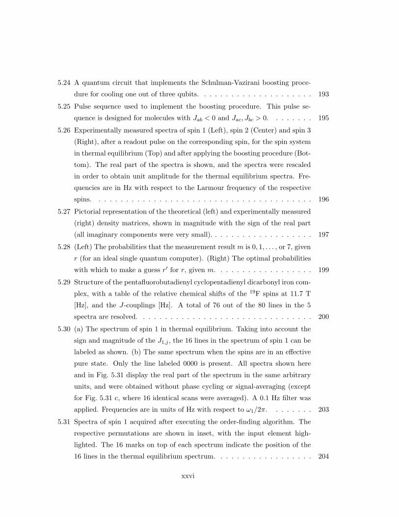
5.26 Experimentally measured spectra of spin 1 (Left), spin 2 (Center) and spin 3
(Right), after a readout pulse on the corresponding spin, for the spin system
in thermal equilibrium (Top) and after applying the boosting procedure (Bot-
tom). The real part of the spectra is shown, and the spectra were rescaled
in order to obtain unit amplitude for the thermal equilibrium spectra. Fre-
quencies are in Hz with respect to the Larmour frequency of the respective
spins. . . . . . . . . . . . . . . . . . . . . . . . . . . . . . . . . . . . . . . . 196
5.27 Pictorial representation of the theoretical (left) and experimentally measured
(right) density matrices, shown in magnitude with the sign of the real part
(all imaginary components were very small). . . . . . . . . . . . . . . . . . . 197
5.28 (Left) The probabilities that the measurement result m is 0, 1, . . . , or 7, given
r (for an ideal single quantum computer). (Right) The optimal probabilities
with which to make a guess r′ for r, given m. . . . . . . . . . . . . . . . . . 199
5.29 Structure of the pentafluorobutadienyl cyclopentadienyl dicarbonyl iron com-
plex, with a table of the relative chemical shifts of the 19F spins at 11.7 T
[Hz], and the J-couplings [Hz]. A total of 76 out of the 80 lines in the 5
spectra are resolved. . . . . . . . . . . . . . . . . . . . . . . . . . . . . . . . 200
5.30 (a) The spectrum of spin 1 in thermal equilibrium. Taking into account the
sign and magnitude of the J1,j , the 16 lines in the spectrum of spin 1 can be
labeled as shown. (b) The same spectrum when the spins are in an effective
pure state. Only the line labeled 0000 is present. All spectra shown here
and in Fig. 5.31 display the real part of the spectrum in the same arbitrary
units, and were obtained without phase cycling or signal-averaging (except
for Fig. 5.31 c, where 16 identical scans were averaged). A 0.1 Hz filter was
applied. Frequencies are in units of Hz with respect to ω1/2π. . . . . . . . 203
5.31 Spectra of spin 1 acquired after executing the order-finding algorithm. The
respective permutations are shown in inset, with the input element high-
lighted. The 16 marks on top of each spectrum indicate the position of the
16 lines in the thermal equilibrium spectrum. . . . . . . . . . . . . . . . . . 204
xxvi

5.32 Outline of the quantum circuit for quantum factorization of the number fif-
teen. The first register of n = 8 qubits is initialized to |0〉 and then put into
the equal superposition∑2n−1
x=0 |x〉 using n Hadamard operations. The sec-
ond register is initialized to |y〉 = |1〉. Then we multiply the second register
by axmod 15 via n controlled multiplications by a2k modulo 15. Next the
Quantum Fourier transform is applied to the first register and the qubits of
the first register are measured. . . . . . . . . . . . . . . . . . . . . . . . . . 205
5.33 Simplified quantum circuit for quantum factorization of the number fifteen. 206
5.34 Quantum circuit for the modular exponentiation. (Left) for a = 11; con-
trolled multiplication of y = 1 by 11 is replaced by controlled addition of
10 to y = 1. (Right) for a = 7; gates A and B correspond to addition of 6
and y = 1 controlled by x0, and gates C through H multiply the result by 7
controlled by x1. As we will see in section 5.10.2, the gates shown in dotted
lines can be left out and the gates shown in dashed lines can be replaced by
similar but simpler gates. . . . . . . . . . . . . . . . . . . . . . . . . . . . . 207
5.35 The seven spin molecule, along with the measured J-coupling constants [Hz],
chemical shifts at 11.7 T [Hz] and relaxation time constants [s]. . . . . . . . 208
5.36 Schematic diagram of the synthesis of the seven-spin molecule. . . . . . . . 208
5.37 Simplified quantum circuit for the modular exponentiation for the “difficult”
case (a = 7). . . . . . . . . . . . . . . . . . . . . . . . . . . . . . . . . . . . 211
5.38 Fluorine spectrum of the seven-spin molecule of Fig. 5.35. The five major
lines correspond )from left to right) to qubits 1, 4, 2, 5, 3. In addition, two
smaller lines from impurities are visible around 25 kHz. The spectrum is
shown in absolute value. Frequencies are given in kHz, with respect to an
arbitrary reference frequency near 470 MHz. . . . . . . . . . . . . . . . . . . 213
5.39 Experimentally measured spectra for the five fluorine spins in thermal equi-
librium. The real part is displayed, in arbitrary units. Frequencies are with
respect to ωi/2π, in Hz. . . . . . . . . . . . . . . . . . . . . . . . . . . . . . 214
5.40 Experimentally measured spectra for the two carbon spins in thermal equi-
librium. The real part is displayed, in arbitrary units. Frequencies are with
respect to ωi/2π, in Hz. . . . . . . . . . . . . . . . . . . . . . . . . . . . . . 215
5.41 Experimentally measured spectra, similar to Fig. 5.39, after preparing all
seven spins in the effective pure ground state. . . . . . . . . . . . . . . . . . 215
xxvii
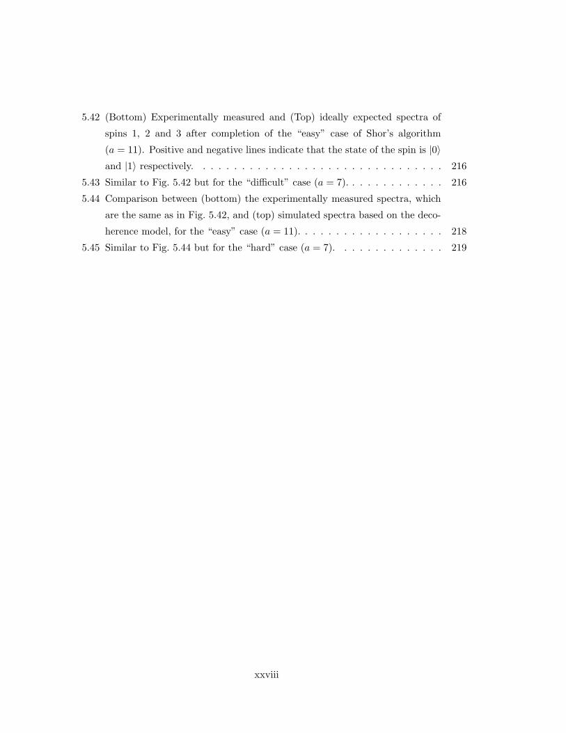
5.42 (Bottom) Experimentally measured and (Top) ideally expected spectra of
spins 1, 2 and 3 after completion of the “easy” case of Shor’s algorithm
(a = 11). Positive and negative lines indicate that the state of the spin is |0〉and |1〉 respectively. . . . . . . . . . . . . . . . . . . . . . . . . . . . . . . . 216
5.43 Similar to Fig. 5.42 but for the “difficult” case (a = 7). . . . . . . . . . . . . 216
5.44 Comparison between (bottom) the experimentally measured spectra, which
are the same as in Fig. 5.42, and (top) simulated spectra based on the deco-
herence model, for the “easy” case (a = 11). . . . . . . . . . . . . . . . . . . 218
5.45 Similar to Fig. 5.44 but for the “hard” case (a = 7). . . . . . . . . . . . . . 219
xxviii

Chapter 1
Introduction
1.1 Historical background
“There is plenty of room at the bottom.” This was the title of a now classic 1959 talk given
by Richard Feynman at the annual meeting of the American Physical Society [Fey60]. In
this talk, Feynman gave physicists and engineers a wonderful challenge: to manipulate and
control things on a small scale. In particular, he challenged his audience to think about
building very small computers, with wires just 10 or 100 atoms in diameter, and circuits just
a few thousand angstroms across. Forty years later, semiconductor technology is rapidly
approaching these dimensions, driven by Moore’s law. But Feynman didn’t mean just small,
he meant really small:
“When we get to the very, very small world — say circuits of seven atoms —
we have a lot of new things that would happen that represent completely new
opportunities for design. Atoms on a small scale behave like nothing on a large
scale, for they satisfy the laws of quantum mechanics. So, as we go down and
fiddle around with the atoms down there, we are working with different laws,
and we can expect to do different things. We can manufacture in different ways.
We can use, not just circuits, but some system involving the quantized energy
levels, or the interactions of quantized spins, etc.”
This is the earliest reference I am aware of that hints at the subject matter of my
thesis work. With reference to his daring ideas, Feynman also made the following crucially
important point:
1
2 CHAPTER 1. INTRODUCTION
“It is not an attempt to violate any laws; it is something, in principle, that can
be done; but in practice, it has not been done because we are too big.”
So what are the laws which limit computation ? How much energy does it take to
compute, and how much time and space does a computation require ?
The relationship between energy consumption and computation has been studied in
detail by Rolf Landauer. In a 1961 paper [Lan61], he showed that the amount of energy
dissipated into the environment when a single bit of information is erased, is at least kBT ln 2,
where kB is Boltzman’s constant and T is the temperature of the environment. As a result,
irreversible logic gates, such as the nand gates in today’s computers, must dissipate a finite
amount of energy, as information is lost when executing the gate (it is not possible to run the
gate backwards and reconstruct the input from the output). Remarkably, Lecerf [Lec63] and
Bennett [Ben73] later showed that it is possible to perform universal computation reversibly,
without ever erasing information, and furthermore that universal computation is possible
without net dissipation of energy.
The time and space resources needed for computation, and in particular how the re-
sources scale with the problem size, are the subject of complexity theory. Arguably the
most significant result of this field, which started with Alan Turing’s introduction of the
Turing machine [Tur36], is the strong Church-Turing thesis [Chu36, Dav65]. It states that
“Any model of computation can be simulated on a probabilistic Turing machine with at most
a polynomial increase in the number of elementary operations required.” As a consequence,
a mechanical machine1 such as Babbage’s difference engine of the 1800’s is polynomially
equivalent to the fastest supercomputer.
Polynomial differences in speed can of course still be significant, and over the past
decades, enormous increases in speed have been realized by making devices that are smaller,
consume less power and are more highly integrated. However, no matter how impressive
the progress, the laws of physics underlying the operation of today’s computers are still the
same as in computers fifty years ago, namely the classical laws of physics.
In the early eighties, the quest for really small computers took on a completely new
face. First, Paul Benioff showed that a quantum mechanical Hamiltonian can represent a
universal (classical) Turing machine [Ben80]. Then Richard Feynman conjectured that a
quantum computer might be able to do more than classical Turing machines; it might for1Provided it has a large enough memory, similar to the tape of a Turing machine.

1.1. HISTORICAL BACKGROUND 3
example efficiently simulate the dynamics of another quantum system [Fey82, Fey85], a feat
which is impossible on classical computers. David Deutsch then fully developed the concept
of a quantum Turing machine and highlighted the potential of quantum computers to speed
up computations via quantum parallellism [Deu85].
Ten years later, the field of quantum computation really took off when Peter Shor
announced his quantum factoring algorithm [Sho94]. This was the first quantum algorithm
exploited quantum parallellism to offer an exponential speed-up over classical machines for
solving an important mathematical problem (prime factorization). Another two years later,
Lov Grover invented a quantum algorithm for unstructured search problems [Gro97] and
Seth Lloyd [Llo96] proved Feynman’s conjecture on quantum simulations.
Despite these spectacular results, the field of quantum computation was regarded with
much scepticism because of the difficulty of maintaining coherent superposition states. How-
ever, much of the scepticism was silenced when Peter Shor [Sho95] and Andrew Steane [Ste96]
discovered quantum error correction and showed that random errors due to decoherence
can in fact be corrected. Furthermore, provided the probability of error per computa-
tional step is low enough, the coding and decoding operations associated with quantum
error correction introduce fewer errors than can be corrected, even with imperfect opera-
tions [ABO97, Kit97, KLZ98].
At this point, the physical realization of quantum computers became another grand
challenge, much like Feynman’s challenge of building a very, very small classical computer:
to build a computer capable of solving problems beyond the reach of classical computers,
by virtue of using quantum mechanical superpositions and entanglement.
Many physical systems have been proposed as potential quantum computers, including
trapped ions [CZ95], cavity quantum electrodynamics [THL+95], electron spins in quantum
dots [LD98], superconducting loops [MOL+99] and nuclear spins [DiV95a]. However, due
to the limited state of the art in any of these experimental techniques, a demonstration
of even the most modest quantum algorithm appeared to be out of reach for a number of
years.
This situation changed completely when Neil Gershenfeld and Isaac Chuang [GC97]
and independently David Cory, Timothy Havel and Amr Fahmy [CFH97] developed an
explicit proposal to build a simple quantum computer using nuclear spins in liquid solution,
requiring only standard nuclear magnetic resonance technology. Fifty five years after nuclear
4 CHAPTER 1. INTRODUCTION
spin states and spin echoes were proposed for (classical) data storage [AGH+55], nuclear
magnetic resonance thus became the workhorse for the early exploration of experimental
quantum computation.
Related fields
In parallel with quantum computation, the related field of quantum information theory de-
veloped, which forms the quantum analogue of classical information theory [CT91]. Quan-
tum information theory describes the notions of a quantum source and a quantum channel,
and studies techniques for quantum source and channel coding. In particular, quantum
information theory sets out to understand how entanglement, which has no classical equiv-
alent, can be used as a resource in communication.
This field has produced spectacular results such as quantum teleportation [BBC+93],
superdense coding [BW92] and quantum cryptography [BB84, Ben92]. Several groups
have already teleported photon states [BPM+97, BBM+98], and secure key distribution
using quantum cryptography has been demonstrated experimentally through optical fibers
over tens of kilometers [MZG96] and through space by daylight over a distance of 1.6 km
[BHL+00] (see [GRTZ01] for a review). Certainly, quantum cryptography is at a more
mature stage than quantum computing.
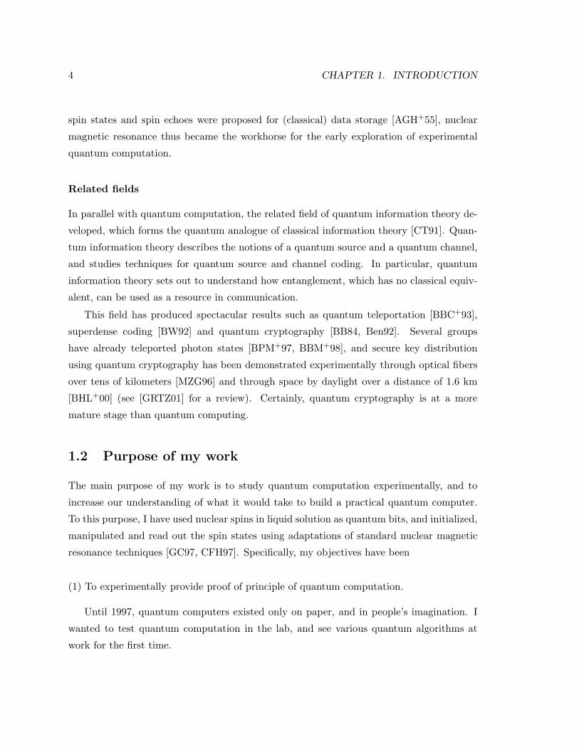
1.2 Purpose of my work
The main purpose of my work is to study quantum computation experimentally, and to
increase our understanding of what it would take to build a practical quantum computer.
To this purpose, I have used nuclear spins in liquid solution as quantum bits, and initialized,
manipulated and read out the spin states using adaptations of standard nuclear magnetic
resonance techniques [GC97, CFH97]. Specifically, my objectives have been
(1) To experimentally provide proof of principle of quantum computation.
Until 1997, quantum computers existed only on paper, and in people’s imagination. I
wanted to test quantum computation in the lab, and see various quantum algorithms at
work for the first time.

1.3. ORGANIZATION OF THE DISSERTATION 5
(2) To stimulate theoretical questions by doing quantum computing experiments.
Interplay between theory and experiment is crucial for the healthy development of any
research field. I hoped to stimulate theoretical thinking about the fundamentals of quan-
tum computing by doing actual experiments. Furthermore, I hoped to interest theorists in
helping with quantum control and in explaining unexpected experimental observations.
(3) To develop techniques for state initialization, coherent quantum control and read out of
quantum states, useful in many implementations of quantum computers.
It is clear that many of the challenges in building quantum computers are similar across
different proposed implementations. Therefore, techniques and solutions invented in the
context of NMR (nuclear magnetic resonance) quantum computing have the potential to
advance other, perhaps more scalable, approaches to the realization of quantum computers.
The general direction of my work has been to push the state of the art towards more
qubits, more gates and more complex algorithms. At each stage, I have conciously paid
attention to all three objectives. The goal was not just to demonstrate “the next algorithm”,
but rather to learn scientifically from the experiment, and in particular to increase our
understanding of how we can meet this wonderful challenge of building a quantum computer,
a computer capable of solving problems beyond the reach of any classical machine.
1.3 Organization of the dissertation
Chapter 2 lays out the principles of quantum computation, introduces quantum circuits
and quantum gates, and explains the operation of quantum algorithms and quantum error
correction. From this theoretical discussion, five requirements for the implementation of
quantum computers naturally emerge. Those are discussed in chapter 3, along with a brief
overview of the state of the art. In chapter 4, we study in detail how those five requirements
can at least in principle be met in liquid solution NMR experiments. Finally, we explore
NMR quantum computing in practice in a series of experiments, presented in chapter 5.
This structure is illustrated in Fig. 1.1.
Additional connections between the chapters are as follows. The selection of topics and
6 CHAPTER 1. INTRODUCTION
Implementation of QC (Ch. 3)
Theory of
NMRQC
QC (Ch.2)Theory of
NMRQC (Ch. 4)
Experiments (Ch. 5)
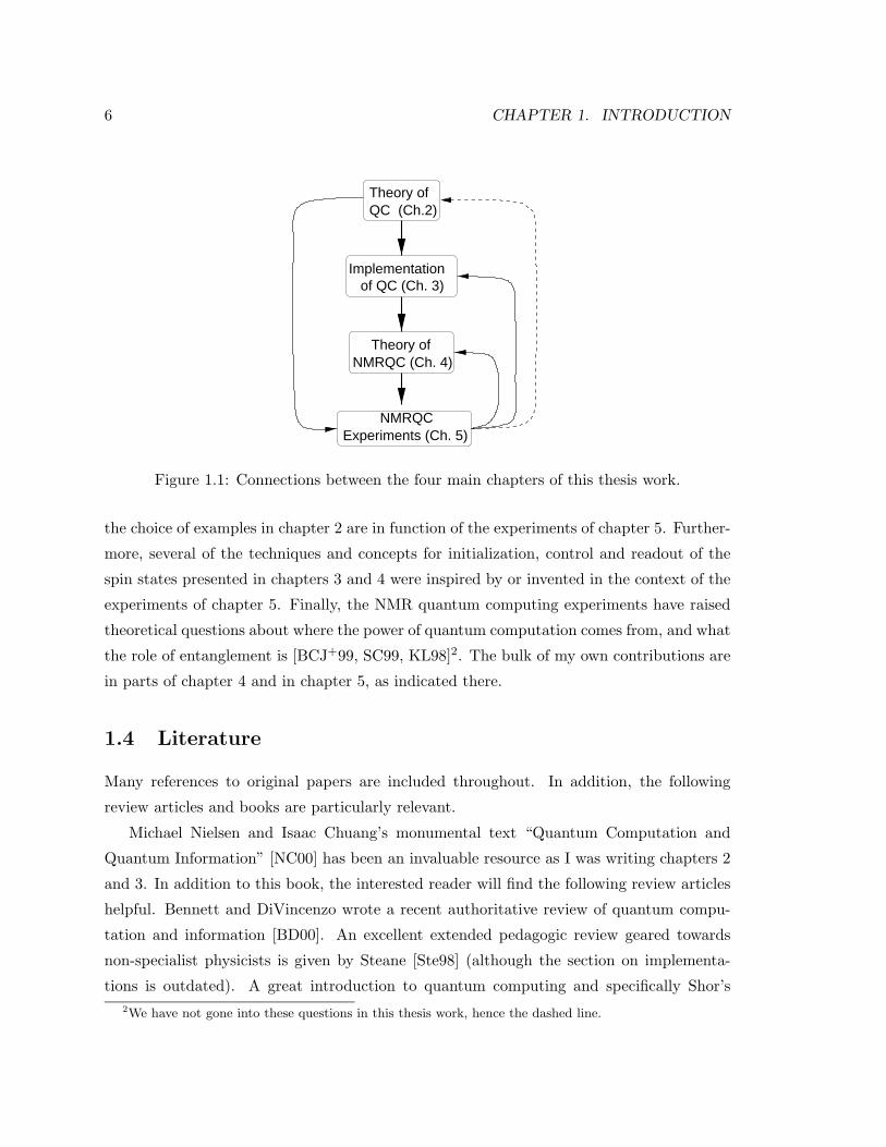
Figure 1.1: Connections between the four main chapters of this thesis work.
the choice of examples in chapter 2 are in function of the experiments of chapter 5. Further-
more, several of the techniques and concepts for initialization, control and readout of the
spin states presented in chapters 3 and 4 were inspired by or invented in the context of the
experiments of chapter 5. Finally, the NMR quantum computing experiments have raised
theoretical questions about where the power of quantum computation comes from, and what
the role of entanglement is [BCJ+99, SC99, KL98]2. The bulk of my own contributions are
in parts of chapter 4 and in chapter 5, as indicated there.
1.4 Literature
Many references to original papers are included throughout. In addition, the following
review articles and books are particularly relevant.
Michael Nielsen and Isaac Chuang’s monumental text “Quantum Computation and
Quantum Information” [NC00] has been an invaluable resource as I was writing chapters 2
and 3. In addition to this book, the interested reader will find the following review articles
helpful. Bennett and DiVincenzo wrote a recent authoritative review of quantum compu-
tation and information [BD00]. An excellent extended pedagogic review geared towards
non-specialist physicists is given by Steane [Ste98] (although the section on implementa-
tions is outdated). A great introduction to quantum computing and specifically Shor’s2We have not gone into these questions in this thesis work, hence the dashed line.

1.4. LITERATURE 7
algorithm, also for physicists, is by Ekert and Jozsa [EJ96], and Lloyd wrote a good intro-
duction for a general audience [Llo95b]. Introductions to a wide array of quantum computer
implementations are compiled in a recent special issue of Fortschritte der Physik [BL00].
Of the many excellent textbooks on quantum mechanics, very few cover the topics most
applicable to quantum computing. Perhaps the most helpful text for understanding the
relevant concepts of quantum mechanics is the great book by Peres [Per93]. Reference
works which cover some of the relevant ideas and notation of quantum mechanics include
Cohen-Tannoudji, Diu and Laloe [CTDL77], Feynman, Leigthon and Sands [FLS65] and
Sakurai [Sak95].
Ray Freeman’s “Spin Choreography” gives a marvelous and intuitive overview of high-
resolution solution NMR techniques and spin dynamics [Fre97]. I found it the most helpful
textbook for the NMR techniques underlying chapter 4. A classic and comprehensive trea-
tise of NMR is Ernst, Bodenhausen and Wokaun [EBW87]. Two other classic texts on
NMR are Slichter [Sli96] and Abragam [Abr61]; both focus on spin physics more than on
spin dynamics.
No textbooks exist specifically on NMR quantum computing, but there are several good
introductory review papers. A good introduction for a general audience is [GC98]. Jonathan
Jones wrote an introductory review for an NMR audience [Jon01], and so did we. We also
wrote an accessible introduction for electrical engineers:
• L.M.K. Vandersypen, C.S. Yannoni, and I.L. Chuang, to appear in The encyclopedia
of NMR (supplement), 2001 [VYC01].
• M. Steffen, L.M.K. Vandersypen, and I.L. Chuang, IEEE Micro, 2001 [SVC01].
Each of the experiments presented in sections 5.3 through 5.9 has been published in
refereed journals. These papers also include many of the techniques presented in chapter 4;
only the technique of section 4.2.5 was published separately.
• 5.3: I. L. Chuang, L. M. K. Vandersypen, X. L. Zhou, D. W. Leung, and S. Lloyd,
Nature, 1998. Reprinted by permission from [CVZ+98] c© (1998) by Macmillan Mag-
azines, Ltd.
• 5.4: D. Leung, L. Vandersypen, X. Zhou, M. Sherwood, C. Yannoni, and I. Chuang,
Phys. Rev. A, 1999. Reprinted by permission from [LVZ+99] c© (1999) by The
American Physical Society.

8 CHAPTER 1. INTRODUCTION
• 5.5: L. M. K. Vandersypen, C. S. Yannoni, M. H. Sherwood, and I. L. Chuang, Phys.
Rev. Lett., 1999. Reprinted by permission from [VYSC99] c© (1999) by The American
Physical Society.
• 5.6: C.S. Yannoni, M.H. Sherwood, L.M.K. Vandersypen, M.G. Kubinec, D.C. Miller,
and I.L. Chuang, Appl. Phys. Lett., 1999. Reprinted by permission from [YSV+99]
c© (1999) by The American Institute of Physics.
• 5.7: L.M.K. Vandersypen, M. Steffen, M. H. Sherwood, C.S. Yannoni, G. Breyta, and
I. L. Chuang, Appl. Phys. Lett., 2000. Reprinted by permission from [VSS+00] c©(2000) by The American Institute of Physics.
• 5.8: D.E. Chang, L.M.K. Vandersypen, and M. Steffen, Chem. Phys. Lett., 2001.
Reprinted by permission from [CVS01] c© (2001) by Elsevier Science.
• 5.9: L.M.K. Vandersypen, M. Steffen, G. Breyta, C.S. Yannoni, R. Cleve, and I. L.
Chuang, Phys. Rev. Lett., 2000. Reprinted by permission from [VSB+00] c©(2000)
by The American Physical Society.
• 4.2.5: M. Steffen, L.M.K. Vandersypen, and I.L. Chuang. J. Magn. Reson., 2000.
Reprinted by permission from [SVC00] c© (2000) by Academic Press.
• 5.10: L.M.K. Vandersypen, M. Steffen, G. Breyta, C.S. Yannoni, M. Sherwood, and
I. L. Chuang, in preparation, 2001 [VSB+01].
Chapter 2
Theory of quantum computation
In this chapter, we review the principles of the theory of quantum computation. From the
outset, the presentation is directed towards a practical appreciation and understanding of
the subject. Our starting point is the notion of quantum bits. We next present the language
of quantum gates and circuits, and use this language to outline the operation of quantum
algorithms and quantum error correction.
2.1 Fundamental concepts
2.1.1 Quantum bits
One quantum bit
In today’s digital computers, information is stored and processed in the form of bits, entities
which can take on only two values: logical zero, 0, or logical one, 1. These are typically
represented by the voltage at a node, or the alignment of a piece of magnetic material, but
any physical system with at least two distinct states can serve to represent a bit, including
two-level quantum systems such as spins-1/2 and polarized photons. The quantum state
|0〉 corresponds to 0 and the state |1〉 corresponds to 1. For a spin-1/2 particle, the two
computational basis states are represented by the spin up and spin down state (|↑〉 or |↓〉),and for photons by the vertical or horizontal polarization state (|l 〉 or |↔〉).
In contrast to classical bits which can only exist as 0 or 1, two-level quantum systems,
9

10 CHAPTER 2. THEORY OF QUANTUM COMPUTATION
called quantum bits or qubits, can also exist in a superposition state of |0〉 and |1〉, mathe-
matically written as
|ψ〉 = a|0〉+ b|1〉 , (2.1)
where a and b are complex numbers satisfying the normalization condition |a|2 + |b|2 = 1.
The overall phase of |ψ〉 is physically irrelevant as it cannot be revealed by any measurement.
Therefore, we can also write |ψ〉 as
|ψ〉 = cosθ
2|0〉+ eiφ sin
θ
2|1〉 , (2.2)
and visualize the state of a qubit as a point on a sphere, called the Bloch sphere, as in
Fig. 2.1. This representation may convey the impression that a qubit is very much like an
analog classical variable, with two degrees of freedom θ and φ. However, as we will see,
qubits are in many ways very different from such analog classical variables. Rather than
pointing along a certain direction, a qubit in a superposition state a|0〉 + b|1〉 is in some
sense in both |0〉 and |1〉 at the same time. Furthermore, as we shall see next, the number
of degrees of freedom in an n-qubit state increases exponentially with n.
|ψ
x
z
y
θ
φ
|0
|1|0 + i
|0 |1+2
|12
(a) (b)
Figure 2.1: (a) Bloch sphere representation of the state |ψ〉 of a single qubit. (b) Theposition in the Bloch sphere of four important states. By convention, we will always let |0〉be along +z.
2.1. FUNDAMENTAL CONCEPTS 11
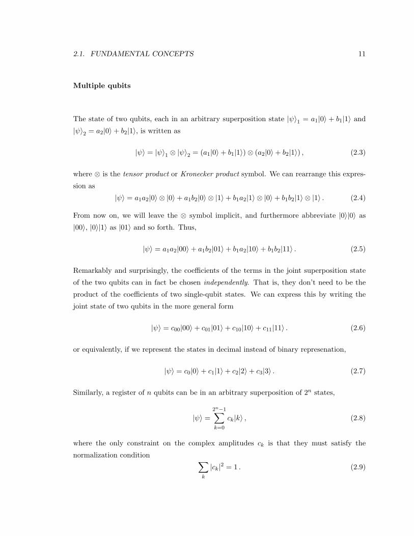
Multiple qubits
The state of two qubits, each in an arbitrary superposition state |ψ〉1 = a1|0〉 + b1|1〉 and
|ψ〉2 = a2|0〉+ b2|1〉, is written as
|ψ〉 = |ψ〉1 ⊗ |ψ〉2 = (a1|0〉+ b1|1〉)⊗ (a2|0〉+ b2|1〉) , (2.3)
where ⊗ is the tensor product or Kronecker product symbol. We can rearrange this expres-
sion as
|ψ〉 = a1a2|0〉 ⊗ |0〉+ a1b2|0〉 ⊗ |1〉+ b1a2|1〉 ⊗ |0〉+ b1b2|1〉 ⊗ |1〉 . (2.4)
From now on, we will leave the ⊗ symbol implicit, and furthermore abbreviate |0〉|0〉 as
|00〉, |0〉|1〉 as |01〉 and so forth. Thus,
|ψ〉 = a1a2|00〉+ a1b2|01〉+ b1a2|10〉+ b1b2|11〉 . (2.5)
Remarkably and surprisingly, the coefficients of the terms in the joint superposition state
of the two qubits can in fact be chosen independently. That is, they don’t need to be the
product of the coefficients of two single-qubit states. We can express this by writing the
joint state of two qubits in the more general form
|ψ〉 = c00|00〉+ c01|01〉+ c10|10〉+ c11|11〉 . (2.6)
or equivalently, if we represent the states in decimal instead of binary represenation,
|ψ〉 = c0|0〉+ c1|1〉+ c2|2〉+ c3|3〉 . (2.7)
Similarly, a register of n qubits can be in an arbitrary superposition of 2n states,
|ψ〉 =2n−1∑k=0
ck|k〉 , (2.8)
where the only constraint on the complex amplitudes ck is that they must satisfy the
normalization condition ∑k
|ck|2 = 1 . (2.9)
12 CHAPTER 2. THEORY OF QUANTUM COMPUTATION
As for single-qubit states, the overall phase is irrelevant. Therefore,
the description of a pure state of n qubits requires 2n − 1 complex numbers.1
This is manifestly different from classical systems. For example, the position of n points on
the sphere of Fig. 2.1 is described by only n rather than 2n complex numbers. In fact, the
position of any n classical particles can always be described by a number of real or complex
numbers that is linear in n.
Since we cannot visualize the state of n qubits via n Bloch spheres, or n points on a single
Bloch sphere, how can we visualize their state? This is difficult — our intuition fails at the
quantum level, because we didn’t grow up with an intuition for quantum mechanics, and
because our observations of the every-day world around us are observations of a classical
world. Mathematically, the extension of the Bloch sphere is called Hilbert space, a 2n
dimensional complex vector space with an inner product. The state of a quantum system
thus corresponds to a point in Hilbert space.
Entanglement
Since the number of degrees of freedom of n quantum systems grows exponentially more
quickly than that of n classical systems, surely there must exist quantum states which have
no classical equivalent. The state of Eq. 2.3 is a classical state: this joint state of two qubits
can be fully described via a description of the individual qubits (which requires one complex
number, or two real numbers, for each qubit). We say that the state of Eq. 2.3 is separable.
In contrast, it is impossible to find two one-qubit states |ψ〉1 = a1|0〉+ b1|1〉 and |ψ〉2 =
a2|0〉+ b2|1〉, such that their tensor product gives the state
|00〉+ |11〉√2
. (2.10)
In other words, this state cannot be written as a product of two one-qubit states. We
call such a state non-separable or entangled. Let us give two more examples: the state12(|00〉− |01〉+ |10〉− |11〉 can be written as 1
2(|0〉+ |1〉)(|0〉− |1〉) and is thus separable; the
state 12(|00〉 + |01〉 + |10〉 − |11〉) cannot be factored into two one-qubit states and is thus
1A mixed state of n qubits has 4n−1 degrees of freedom. The distinction between pure and mixed stateswill be discussed shortly.
2.1. FUNDAMENTAL CONCEPTS 13
entangled.
Mixed states versus pure states
A quantum system in a well-defined and well-known state |ψ〉 is said to be in a pure state.
If all we know about a quantum system is that it is in one of several pure states |ψi〉, each
with certain probabilities pi, we say the quantum system is in a statistical mixture of these
pure states, or for short that it is in a mixed state. The state of a quantum system in a
statistical mixture is conveniently described by its density operator
ρ =∑i
pi|ψi〉〈ψi| , (2.11)
where 〈ψ| represents the Hermitian conjugate of |ψ〉, and |ψ〉〈φ| denotes the outer product
(a linear operator). Obviously, the probabilities pi must satisfy pi ≥ 0 and∑
i pi = 1. For
a pure state |ψ〉, the density operator is simply ρ = |ψ〉〈ψ|.
Every density operator satisfies
Tr(ρ) = 1 , (2.12)
since Tr(ρ) =∑
i piTr(|ψi〉〈ψi|) =∑
i pi. Furthermore, the eigenvalues λj of ρ satisfy
λj ≥ 0 , (2.13)
so ρ is a positive operator, and one can decompose it as
ρ =∑j
λj |j〉〈j| , (2.14)
where the |j〉 are orthogonal eigenvectors of ρ (the |ψi〉 of Eq. 2.11 need not be orthogonal).
We can thus also interpret a quantum system in ρ to be in the state |j〉 with probability λj ,
and make the important observation that an arbitrary density matrix does thus not have a
unique decomposition into any specific mixture of states.
The mathematical distinction between pure and mixed states is that a pure state den-
sity operator has only one non-zero eigenvalue (necessarily equal to 1), whereas a mixed
state density operator has more than one non-zero eigenvalue. It follows that a convenient

14 CHAPTER 2. THEORY OF QUANTUM COMPUTATION
criterion to distinguish pure and mixed states is
Tr(ρ2) = 1 ⇔ ρ is pure (2.15)
Tr(ρ2) < 1 ⇔ ρ is mixed . (2.16)
Of course, any quantum system is really in just one state. We emphasize therefore, that
to say that a quantum system is in a mixed state is merely a statement about our knowledge
of the state of the quantum system. As we shall see, the distinction between pure and mixed
states has important implications — pure states are in many respects more “useful” than
mixed states.
Promise of qubits
It may appear at first sight that a bit which is simultaneously 0 and 1 is not very useful
for computation, and is, in fact, rather confusing. However, the exponential complexity
of quantum systems also suggests that perhaps quantum bits could be immensely useful
for computation. This observation led Richard Feynman to speculate that “quantum com-
puters” might be able to solve certain problems exponentially faster than any classical
machine [Fey85, Fey96]. In the next section, we first verify that quantum systems can in-
deed be used for computation. In the following section we explore the potential of quantum
superpositions and entanglement for performing massively parallel computations.
2.1.2 Computation using quantum systems
So far, we have merely given a static description of quantum bits as two-level quantum
systems which can hold information in binary form. We will now look at the dynamics of
quantum bits, and examine whether we can perform computations by evolving the state of
a set of quantum systems in a controlled way.
Unitary evolution
One of the postulates of quantum mechanics dictates that the time evolution of the state
|ψ(t)〉 of a closed quantum system (i.e. a system which does not interact with the environ-
ment, the rest of the universe) is governed by Schrodinger’s equation:
i~d|ψ(t)〉dt
= H|ψ(t)〉 , (2.17)
2.1. FUNDAMENTAL CONCEPTS 15
where ~ is Plank’s constant and H is the Hamiltonian, an operator for the total energy of
the system. For time-independent Hamiltonians, the Schrodinger equation has a straight-
forward solution:
|ψ(t)〉 = exp(−iHt~
) |ψ(t = 0)〉 . (2.18)
If the Hamiltonian is time-dependent, the Schrodinger equation has no easy solution, al-
though the evolution can be approximated as a sequence of evolutions under time-independent
Hamiltonians. We usually denote the time-evolution operator as U , where
U = exp(−iHt~
) , (2.19)
so
|ψ(t)〉 = U |ψ(0)〉 . (2.20)
Similarly, the time evolution of the density operator ρ of a quantum system is
ρ(t) =∑i
pi|ψi(t)〉〈ψi(t)| =∑i
pi U |ψi(0)〉〈ψi(0)| U † = Uρ(0) U † , (2.21)
where the † symbol indicates the Hermitian conjugate.
From Eq. 2.18, we can appreciate the important role of the Hamiltonian of a quantum
system: it controls the time evolution of the quantum system. Since H is a Hermitian
operator, i.e. it is its own Hermitian conjugate H = H†, the time evolution operator
U = exp(−iHt/~) is unitary, that is UU † = e−iHt/~eiH†t/~ = I = eiH
†t/~e−iHt/~ = U †U .
This implies that the evolution of a closed quantum system is completely reversible . Indeed,
we can unwind any time evolution U by a subsequent time evolution U †.
Geometrically, we can visualize the unitary evolution of a single qubit as a rotation in
the Bloch sphere (Fig. 2.1), a picture we will often use in chapter 4. By extension, the
unitary evolution of multiple qubits corresponds to a rotation in Hilbert space.
Irreversible and reversible computation
Today’s classical computers do not at all operate in a reversible manner. Note for example
that your computer generates heat. Also note that it is not possible to reconstruct the input
of a traditional and gate from its output (Fig. 2.2 a). This is obvious since the and gate
has two input bits and only one output bit; it is never possible to reconstruct the value of

16 CHAPTER 2. THEORY OF QUANTUM COMPUTATION
two bits starting from only one bit. But even if we introduce a second output bit (Fig. 2.2
b), it is not possible to make the and gate reversible. This is because the and gate is not
single-valued. If the output is 00 in the example of Fig. 2.2 b, we cannot know whether the
input was 00 or 01.
It is thus natural to ask whether universal computation can be done reversibly. Rolf
Landauer and Charles Bennett showed that indeed any computation can be performed
in a completely reversible manner, that is without (or with infinitesimal) energy dissipa-
tion [Lan61][Ben73]. The only time heat must be dissipated is in the process of resetting
a bit, which irreversibly erases the information contained in the bit and thus necessarily
increases the entropy.
In Out0 0 00 1 01 0 01 1 1
In Out0 0 0 00 1 0 01 0 1 01 1 1 1
In Out0 0 0 0 0 00 1 0 0 1 01 0 0 1 0 01 1 0 1 1 10 0 1 0 0 10 1 1 0 1 11 0 1 1 0 11 1 1 1 1 0(a) (b)
(c)
Figure 2.2: Truth table for (a) The traditional and gate; the output is 1 when both inputsare 1, and the output is 0 otherwise. (b) The extended and gate, with two output bits. (c)A reversible and gate, also known as the Toffoli gate.
Any multi-valued function f ,
x 7→ f(x) (2.22)
can be made reversible by introducing a second input bit string y of the same length as
f(x) and extending Eq. 2.22 to
(x, y) 7→ (x, y ⊕ f(x)) , (2.23)
where ⊕ is the bitwise addition modulo two (equivalent to the bitwise xor). If we set y to
0, we simply obtain f(x) in the second register:
(x, 0) 7→ (x, f(x)) . (2.24)
2.1. FUNDAMENTAL CONCEPTS 17
We can thus construct a reversible version of the and gate for example, by using an addi-
tional input bit (Fig. 2.2 c). The third bit is always initialized to 0, so in practice only the
top half of the truth table is ever used. The input can now always be reconstructed from
the output. Similarly, if we initialize the third bit to 1, and thus use only the bottom half
of the truth table of Fig. 2.2 c, we obtain a nand gate. Since the nand gate is universal
for classical logic, the Toffoli is universal for reversible classical computation [Tof80].
We will return to the implementation of quantum computers in chapter 3. For now,
we will just state that it may be possible to control the Hamiltonian in such a way that
the time evolution results in a transformation of the qubit states which corresponds to the
transformation of bit values in a classical truth table [Ben80]. That is, the computational
basis states of the qubits (|0〉 or |1〉 for each qubit) can be transformed as
|x〉 7→ |f(x)〉 (2.25)
for reversible f , or, by extension, as
|x〉|y〉 7→ |x〉|y ⊕ f(x)〉 , (2.26)
for irreversible f , corresponding to Eqs. 2.22 and 2.23 respectively. Therefore, we can say
that
quantum computation subsumes classical computation.
Now, what would happen if the quantum bits were initially in a superposition state of the
computational basis states,∑2n−1
k=0 ck|k〉 ? This is the subject of the next section.
2.1.3 Quantum parallellism
Quantum parallellism
Every computation can be seen as the concatenation of many logic gates. Each logic gate
produces an output which is a function of its input. Now consider a classical and reversible2
logic gate which implements a function f with one input bit x and one output bit y = f(x).
If x = 0, the gate will output f(0), and if x = 1, the gate will output f(1). Now imagine we
can implement an analogous quantum logic gate, which transforms a qubit as |x〉 7→ |f(x)〉.2If f is not reversible, we know how to make it reversible from section 2.1.2.

18 CHAPTER 2. THEORY OF QUANTUM COMPUTATION
By virtue of the linearity of quantum mechanics, the same quantum gate transforms a qubit
in a superposition state as
a|0〉+ b|1〉 f7→ a|f(0)〉+ b|f(1)〉 . (2.27)
In some sense, the function f has been evaluated for both its input values (0 and 1) in one
step! Next consider a different logic gate which implements a function f with two input
and two output bits. If we prepare the two qubit system in the state
|ψ〉 = a|00〉+ b|01〉+ c|10〉+ d|11〉 , (2.28)
evaluation of the function f tranforms the state to
a|f(00)〉+ b|f(01)〉+ c|f(10)〉+ d|f(11)〉 , (2.29)
so f has been evaluated for four input values in parallel. For every additional input bit, the
potential number of parallel function evaluations doubles! In general, a function of n bits
implemented on a quantum computer can be evaluated for all 2n possible input values at
the same time:2n−1∑x=0
|x〉 f7→2n−1∑x=0
|f(x)〉 , (2.30)
where x is an integer encoded by a string of n bits. Thus, whereas for classical computers
the number of parallel function evaluations increases at best linearly with their size,
the number of parallel function evaluations grows exponentially with the size of
the quantum computer (the number of qubits).
This truly spectacular notion was first introduced by David Deutsch in 1985, and termed
quantum parallellism [Deu85].
Machines based on quantum bits thus appear to be exponentially more powerful than
any machine using just classical bits. Of course, a computation is only meaningful if the
output result can be read out, but how do we measure the state of quantum bits, and just
what does the measurement give when the qubit is in a superposition state?
2.1. FUNDAMENTAL CONCEPTS 19
Measurement of quantum states
The postulates of quantum mechanics dictate that any measurement of a quantum system
can be described in terms of a set of measurement operators Pm. Measurement of a quan-
tum system in the state |ψ〉 immediately before the measurement gives outcome m with
probability
p(m) = 〈ψ|Pm|ψ〉 . (2.31)
The state of the quantum system after the measurement is
Pm|ψ〉〈ψ|Pm|ψ〉
. (2.32)
The measurement operators must satisfy the completeness relation
∑m
Pm = I , (2.33)
such that the probabilities pm sum to 1. Furthermore, for a projective measurement, we
also require that the operators Pm be Hermitian and that
PmPm′ = δmm′Pm . (2.34)
We can therefore associate an orthonormal basis of states |m〉 with any set of projective
measurement operators Pm, such that Pm = |m〉〈m|. Then, the probability of obtaining m
in a measurement of a quantum system in |ψ〉 is p(m) = |〈m|ψ〉|2 (note that 0 ≤ pm ≤ 1,
with equality only if |ψ〉 = |m〉), and the post-measurement state is |m〉.For example, if we measure a single qubit in the state |0〉 in the |0〉, |1〉 basis (the
computational basis), the measurement always gives 0. If we measure a qubit in a|0〉+ b|1〉in the same basis, we obtain 0 with probability |a|2 and 1 with probability |b|2.
What happens if we measure a qubit in |ψ〉 = a|0〉 + b|1〉 twice in a row, in the same
basis? From Eqs. 2.32 and 2.34, we see that the result of the second measurement will
always be identical to the result of the first measurement. The first measurement will give
m and in the process collapses 3 |ψ〉 onto the corresponding measurement basis state |m〉.Since the |m〉 are orthogonal, the second measurement will with certainty return m as well.
3Collapse is only one of several interpretations of the measurement process. Since they all make the samepredictions for the measurement statistics and outcomes, we will not concern ourselves with interpretationissues.

20 CHAPTER 2. THEORY OF QUANTUM COMPUTATION
Collapse of the quantum state implies that the information contained in the coefficients
a and b is instantaneously and irreversibly destroyed. As a result, an unknown quantum
state cannot be fully characterized even by repeated measurements, whether they take place
in the same basis or in different bases. A second measurement of a qubit in a different basis
than the first measurement will project the state (which now is |m〉, that is |0〉 or |1〉 in
our example) onto the new measurement basis (for example the |0〉+|1〉√2
,|0〉−|1〉√
2 basis).
This measurement does not yield any extra information about |ψ〉, however, because a and
b have already been irretrievably lost; the second measurement is a measurement on the
state |m〉, not on |ψ〉.It would be possible to determine a and b with good accuracy by performing a properly
designed series of measurements on a large number of copies of the qubit in the same un-
known state. However, the no-cloning theorem [Die82, WZ82] forbids the creation of copies
of a qubit in an unknown state (it is of course possible to create many copies of a qubit in
a known state). In summary,
no measurement can fully reveal the state of a qubit in an unknown state.
Furthermore, Eq. 2.31 implies that it is not possible to reliably distinguish two non-
orthogonal quantum states |ψ1〉 and |ψ2〉: regardless of the basis we choose, there must be a
|m〉 for which 〈ψ1|m〉2 6= 0 and 〈ψ2|m〉2 6= 0. Orthogonal states in contrast, can be perfectly
distinguished by a measurement in the appropriate basis.
We note that while the evolution of a closed quantum system is unitary (see sec-
tion 2.1.2), the measurement process inherently invokes an interaction with an external
measuring device during which the quantum system cannot remain closed. As a result, the
measurement process is non-unitary; it constitutes a projection onto a finite set of basis
states in Hilbert space, rather than a rotation in Hilbert space.
Finally, we point out that we have restricted ourselves to projective measurements,
also known as hard measurements. We postpone a discussion of weak measurements until
section 3.1.4 and apply it to the case of NMR in section 4.5.
Hidden variables and measurements on entangled particles
In light of the measurement process, it is natural to ask what the meaning of superpositions
is. Indeed, if upon measurement we obtain only one of the terms in a superposition, wasn’t

2.1. FUNDAMENTAL CONCEPTS 21
the qubit perhaps already in the corresponding state all along, instead of in several states
“at the same time” ? Isn’t there some hidden variable which predetermines what the mea-
surement outcome will be ? This question has been the subject of much debate throughout
the 20th century (for a good introduction, see [Mer85]).
In a 1935 paper, Einstein, Podolsky and Rosen (EPR) considered what would happen if
a measurement is performed on one of two entangled particles [EPR35]. Suppose we prepare
two qubits in the entangled state 1√2|01〉− 1√
2|10〉 (the singlet state, one of the four so-called
EPR states). If we measure qubit 1 in the computational basis, the outcome will be |0〉 or
|1〉. Now, what would be the result of a subsequent measurement of qubit 2? Because of
the entanglement, the wavefunction of both particles collapses to either |01〉 or |10〉 upon
measuring the first qubit, and therefore the outcome for the second qubit will always be
opposite to the outcome of the first qubit. In fact, for the singlet state, the outcomes
for the two particles will be opposite for a measurement in any basis. Furthermore, this
is true even if the two entangled qubits are lightyears away from each other! Actions in
one location would thus appear to have instanteneous consequences for observations in a
different location. Einstein rejected this “spooky action at a distance” calling it absurd. He
believed that quantum theory was incomplete and had to be supplemented with a theory
of local hidden variables.
In 1964, John Bell proposed an actual experiment which would either confirm or dis-
prove local hidden variably theories [Bel64] 4. This experiment was carried out in 1980 by
Alain Aspect [AGR81], and has been repeated many times since then, in attempts to close
more and more possible loopholes in the experiment. The experimental observations have
consistently refuted the existence of local hidden variables, thereby confirming the validity
of quantum theory.
Implications of quantum measurements for quantum parallellism
Returning to quantum parallellism, we see that measurement of two qubits in a superposi-
tion state such as in Eq. 2.29, collapses the state of the qubits and probabilistically returns
f(00), f(01), f(10) or f(11). In general, after performing a phenomenal number of parallel
function evalutions (2n for n qubits), as in Eq. 2.30, a measurement of the final state will
probabilistically give one of the 2n terms in the output superposition state. It thus appears
4Or to be precise, that hidden variables can only exist if information can travel faster than light, whichwe strongly believe is not the case.
22 CHAPTER 2. THEORY OF QUANTUM COMPUTATION
that the exponential computational power of quantum computers is not accessible!
Remarkably, special quantum algorithms exist which allow one to take advantage of
the exponential complexity of quantum systems and circumvent the limitations of quantum
measurements and readout, in order to signficantly speed up certain computational tasks.
2.1.4 Quantum algorithms
Quantum algorithms allow one to take advantage of quantum parallellism and thereby solve
certain problems in far fewer steps than is possible classically.
Notions from complexity theory
The basis for comparison of the power of quantum and classical computers is provided by
complexity theory, which analyzes how the minimal physical resources (time, space, energy)
required for an algorithm to solve a given problem vary with the problem size n [HU79].
The key distinction is whether the resources required are polynomial or exponential in n.
Adding two n digit numbers, for example, can be done in O(n) (a linear function of
n) elementary operations such as nand gates. In contrast, factoring an n digit integer
number into prime numbers is a task for which the best known classical algorithms require
exponentially many operations, about O(en1/3
) [Knu98].
Computer scientists call an algorithm efficient if the required resources grow only poly-
nomially with the problem size, and call it inefficient if the resources increase exponentially.
Problems for which there exist efficient algorithms are called tractable. Problems for which
no efficient algorithm exists are called intractable or hard.
In order to drive home the significance of intractibility, consider the travelling salesman
problem, which is provably intractable classically. Suppose that on a fast computer it takes
one second to find the shortest path connecting 100 cities. For 101 cities, it would then
take two seconds, for 102 cities four seconds and so forth. It would then take over an hour
to find the shortest path through 112 cities, and over a year for only 125 cities. The same
fast computer would need over 35 billion years to solve the travelling salesman problem for
only 160 cities, longer than the estimated age of the universe . . .
2.1. FUNDAMENTAL CONCEPTS 23
Quantum algorithms
The extraordinary promise of quantum computing is that
certain problems which appear intractable on any classical computer are tractable on a
quantum computer.
Factorization of integers into products of prime numbers is an example of such a problem.
This problem is believed to be intractable on any classical machine (although this remains
to be proven): a 400-digit integer cannot be factored with high probability of success in a
reasonable time, not with a handheld calculator, not with a personal computer, not with a
supercomputer, and not using all the fastest supercomputers combined.
However, in 1994, almost 10 years after Deutsch introduced quantum parallellism, Pe-
ter Shor stunned the world with an efficient quantum algorithm for prime factorization
and computation of discrete logarithms [Sho94, Sho97]. The practical importance of this
algorithm is that it could be used to break widely used cryptographic codes, such as the
RSA public key cryptographic system [RSA78]. These codes are based precisely on the fact
that no efficient (classical) algorithm is known for factoring. At a more fundamental level,
Shor’s algorithm is the most powerful example of how quantum mechanics offers a new way
of thinking about information and computation. As a result, the announcement of Shor’s
algorithm gave a tremendous boost to the interest in quantum computing of both funding
agencies and scientists.
Historically, the first quantum algorithm was invented by David Deutsch and Richard
Jozsa (1992) [DJ92]. This algorithm allows a quantum computer to solve with certainty
an artificial mathematical problem known as Deutsch’s problem. It provided the first steps
towards Simon’s algorithm [Sim94, Sim97], and later to Shor’s algorithm. Furthermore, it
is important as a simple quantum algorithm that can be experimentally tested.
Another class of quantum algorithms was discovered in 1996 by Lov Grover [Gro96,
Gro97]. These algorithms allow a quadratic speed-up of unstructured search problems, for
which there is no better approach classically than to try all L candidate solutions one at a
time. A quantum computer using Grover’s algorithm needs to make only√L such trials.
Even though this speed-up is only quadratic rather than exponential, it is still significant.
The last currently known algorithmic application of quantum computers lies in the
simulation of other quantum systems [Llo96], as Feynman conjectured. Even a computer
24 CHAPTER 2. THEORY OF QUANTUM COMPUTATION
consisting of no more than a few dozen quantum bits could outperform the fastest classical
computers in solving relevant physics problems, such as calculating the energy levels of an
atom.
Scope of quantum computing
We close with two final remarks on quantum algorithms.
1. Quantum computing cannot offer any speed-up at all for many common tasks, such
as adding up two numbers or word processing, which can already be done efficiently
on a classical computer.
2. There are many problems which are classically intractable, but for which no efficient
quantum algorithm is possible either [BBBV97].
An efficient quantum algorithm for the travelling salesman problem or a similar prob-
lem would have an enormous impact in the computer science community and the computer
industry. Whether or not such a breakthrough will be made, it would be somewhat dis-
appointing from a practical viewpoint if no other applications of quantum computers were
found than the ones currently known. Either way, it is for certain that the developments
in quantum computation have dramatically changed our understanding of the connection
between physics, information and computation.
We gave here only a brief summary of the known quantum algorithms. Section 2.3
explains the operation and steps of the Deutsch-Jozsa algorithm, Grover’s algorithm and
Shor’s algorithm in detail. We will present experimental implementations of simple instances
of each of these algorithms in chapter 5.
2.1.5 Correcting quantum errors
Quantum errors or decoherence
Quantum parallellism and quantum algorithms inherently rely on quantum mechanical su-
perpositions. However, in real quantum systems, superposition states are preserved only
for a limited time: quantum bits gradually loose coherence due to unavoidable interactions
with the environment, so the information stored in the coefficients of the terms in a super-
position is lost. The environment in a sense acts as a measuring device which alters the
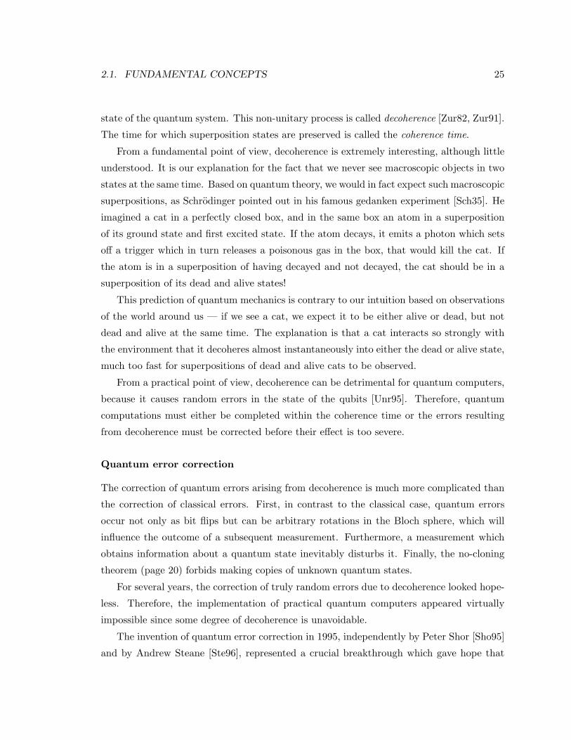
2.1. FUNDAMENTAL CONCEPTS 25
state of the quantum system. This non-unitary process is called decoherence [Zur82, Zur91].
The time for which superposition states are preserved is called the coherence time.
From a fundamental point of view, decoherence is extremely interesting, although little
understood. It is our explanation for the fact that we never see macroscopic objects in two
states at the same time. Based on quantum theory, we would in fact expect such macroscopic
superpositions, as Schrodinger pointed out in his famous gedanken experiment [Sch35]. He
imagined a cat in a perfectly closed box, and in the same box an atom in a superposition
of its ground state and first excited state. If the atom decays, it emits a photon which sets
off a trigger which in turn releases a poisonous gas in the box, that would kill the cat. If
the atom is in a superposition of having decayed and not decayed, the cat should be in a
superposition of its dead and alive states!
This prediction of quantum mechanics is contrary to our intuition based on observations
of the world around us — if we see a cat, we expect it to be either alive or dead, but not
dead and alive at the same time. The explanation is that a cat interacts so strongly with
the environment that it decoheres almost instantaneously into either the dead or alive state,
much too fast for superpositions of dead and alive cats to be observed.
From a practical point of view, decoherence can be detrimental for quantum computers,
because it causes random errors in the state of the qubits [Unr95]. Therefore, quantum
computations must either be completed within the coherence time or the errors resulting
from decoherence must be corrected before their effect is too severe.
Quantum error correction
The correction of quantum errors arising from decoherence is much more complicated than
the correction of classical errors. First, in contrast to the classical case, quantum errors
occur not only as bit flips but can be arbitrary rotations in the Bloch sphere, which will
influence the outcome of a subsequent measurement. Furthermore, a measurement which
obtains information about a quantum state inevitably disturbs it. Finally, the no-cloning
theorem (page 20) forbids making copies of unknown quantum states.
For several years, the correction of truly random errors due to decoherence looked hope-
less. Therefore, the implementation of practical quantum computers appeared virtually
impossible since some degree of decoherence is unavoidable.
The invention of quantum error correction in 1995, independently by Peter Shor [Sho95]
and by Andrew Steane [Ste96], represented a crucial breakthrough which gave hope that
26 CHAPTER 2. THEORY OF QUANTUM COMPUTATION
practical quantum computers may be feasible. The main steps in quantum error correction
are the same as in classical error correction: encoding, a noisy process, decoding, correc-
tion (Fig. 2.3). Despite this similar general outline, the difficulties in correcting quantum
errors require fundamentally different solutions. These principles will be made explicit in
section 2.4, where we explore quantum error correction in more detail.
messageencodedmessage noisy
corruptedmessage
correctchanneldecode &
encodemessage
Figure 2.3: A message (one or more bits or qubits) is first redundantly encoded, the encodedmessage then goes through the process of interest (transmission over a noisy channel, acomputation subject to errors, etcetera), and finally the corrupted encoded message isdecoded and corrections are made if needed, based on the error syndrome (informationabout which errors occurred, contained in the redudancy bits.
Compared to the classical case, quantum error correction involves an even greater over-
head: encoding, decoding and correction require many additional qubits and operations.
An important question then is whether quantum error correction actually corrects for more
errors than it introduces, when the operations are carried out with faulty components. The
answer [ABO97, Kit97, KLZ98], a second key result for quantum computation, was that
provided the error rate (probability of error per elementary operation) is below
a certain threshold, and given a fresh supply of qubits in |0〉, it is possible to
perform arbitrarily long quantum computations.
The critical threshold is called the accuracy threshold . It is currently estimated to be
between 10−4 and 10−6, depending on the assumptions made about the nature of the errors
and the process of interest.
2.2 Quantum gates and circuits
Any algorithm consists of a sequence of steps; in quantum algorithms, each step is a unitary
transformation, Uk. In theory, we could implement the unitary transformation for each step,
Uk, by letting the qubits evolve under the Hamiltonian i lnUk/∆t for a duration ∆t (we recall
Eq. 2.19). In actual experiments, it is often not practical to turn on arbitrary Hamiltonians.
2.2. QUANTUM GATES AND CIRCUITS 27
Fortunately, as we will see, a small set of Hamiltonians is sufficient to generate arbitrary
unitary transformations.
A convenient description of the steps in quantum algorithms at an intermediate level of
abstraction is based on quantum gates, analogous to classical logic gates such as the not,
and and xor gates. In this section, we will
1. describe quantum gates which can be directly implemented on realistic quantum com-
puters,
2. provide a universal set of implementable quantum gates,
3. present methods to decompose complex quantum gates into sequences of directly-
implementable gates, and
4. introduce the quantum circuit notation for the relevant quantum gates (quantum
circuits are diagrams which represent a sequence of quantum gates applied to one or
more qubits) [Deu89, Yao93].
The first three points are the subject of the following three subsections. The fourth
point will be covered throughout this section.
2.2.1 Directly implementable quantum gates
The Hamiltonians present in simple quantum systems contain single-particle terms and
interaction terms between two particles; three-particle terms are normally not observed.
Therefore, the only quantum gates which we can easily implement directly are gates which
act on one or two particles. If each particle represents a qubit, as we shall assume for now,
we can thus realize one- and two-qubit gates directly.
One-qubit gates
Let us first introduce a convenient matrix representation in which to describe quantum
states and unitary transformations. The quantum state |ψ〉 = a|0〉 + b|1〉 is written in
matrix notation as
|ψ〉 =[a
b
], (2.35)
a column vector containing the complex amplitudes of the |0〉 and |1〉 terms. The matrix
representation of 〈ψ| is the complex conjugate of the transpose of the vector |ψ〉. The inner

28 CHAPTER 2. THEORY OF QUANTUM COMPUTATION
product 〈ψ1|ψ2〉 and the outer product |ψ1〉〈ψ2| can be computed as the respective products
of the corresponding column and row matrices.
Now let us consider the simplest building block of quantum computation, a one-qubit
quantum gate, called the not gate. It maps |0〉 onto |1〉 and vice versa, similar to classical
inversion. The unitary matrix which effects this transformation for arbitrary input states is
Unot =[ 0 1
1 0
]. (2.36)
The action of a unitary operator U on a quantum state |ψ〉,
|ψ〉final = U |ψ〉initial , (2.37)
can be calculated by standard matrix multiplication. For example, the output state obtained
after applying Unot to |ψ〉 of Eq. 2.35 is
Unot |ψ〉 =[ 0 1
1 0
] [a
b
]=[b
a
], (2.38)
which is the state vector corresponding to the state a|1〉+ b|0〉, as expected given Eq. 2.27.
The rest of the discussion of one-qubit gates expands on the following notion: any
one-qubit unitary operator can be written in the form
U = eiαRn(θ) , (2.39)
where Rn(θ) corresponds to a rotation in the Bloch sphere (Fig. 2.1) about the n =
(nx, ny, nz) axis and over an angle θ. If there is ambiguity about which qubit R acts on,
we use a superscript to indicate the label of the qubit, Rin(θ). In order to give an explicit
definition of Rn(θ), let us define the usual Pauli matrices
σx ≡[ 0 1
1 0
], σy ≡
[ 0 −ii 0
], σz ≡
[ 1 0
0 −1
], (2.40)
which obey the relations
σxσy = iσz , σxσz = −iσy , σyσz = iσx , (2.41)
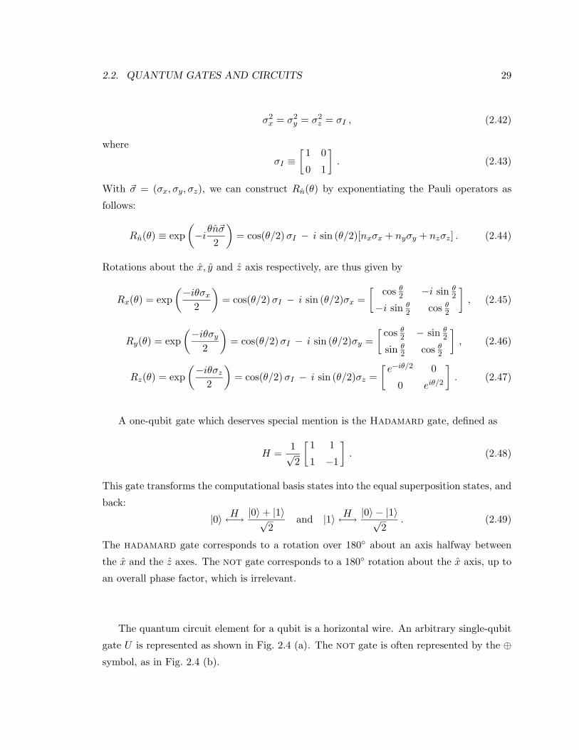
2.2. QUANTUM GATES AND CIRCUITS 29
σ2x = σ2
y = σ2z = σI , (2.42)
where
σI ≡[ 1 0
0 1
]. (2.43)
With ~σ = (σx, σy, σz), we can construct Rn(θ) by exponentiating the Pauli operators as
follows:
Rn(θ) ≡ exp(−iθn~σ
2
)= cos(θ/2)σI − i sin (θ/2)[nxσx + nyσy + nzσz] . (2.44)
Rotations about the x, y and z axis respectively, are thus given by
Rx(θ) = exp(−iθσx
2
)= cos(θ/2)σI − i sin (θ/2)σx =
[ cos θ2 −i sin θ2
−i sin θ2 cos θ2
], (2.45)
Ry(θ) = exp(−iθσy
2
)= cos(θ/2)σI − i sin (θ/2)σy =
[ cos θ2 − sin θ2
sin θ2 cos θ2
], (2.46)
Rz(θ) = exp(−iθσz
2
)= cos(θ/2)σI − i sin (θ/2)σz =
[e−iθ/2 0
0 eiθ/2
]. (2.47)
A one-qubit gate which deserves special mention is the Hadamard gate, defined as
H =1√2
[ 1 1
1 −1
]. (2.48)
This gate transforms the computational basis states into the equal superposition states, and
back:
|0〉 H←→ |0〉+ |1〉√2
and |1〉 H←→ |0〉 − |1〉√2
. (2.49)
The hadamard gate corresponds to a rotation over 180 about an axis halfway between
the x and the z axes. The not gate corresponds to a 180 rotation about the x axis, up to
an overall phase factor, which is irrelevant.
The quantum circuit element for a qubit is a horizontal wire. An arbitrary single-qubit
gate U is represented as shown in Fig. 2.4 (a). The not gate is often represented by the ⊕symbol, as in Fig. 2.4 (b).
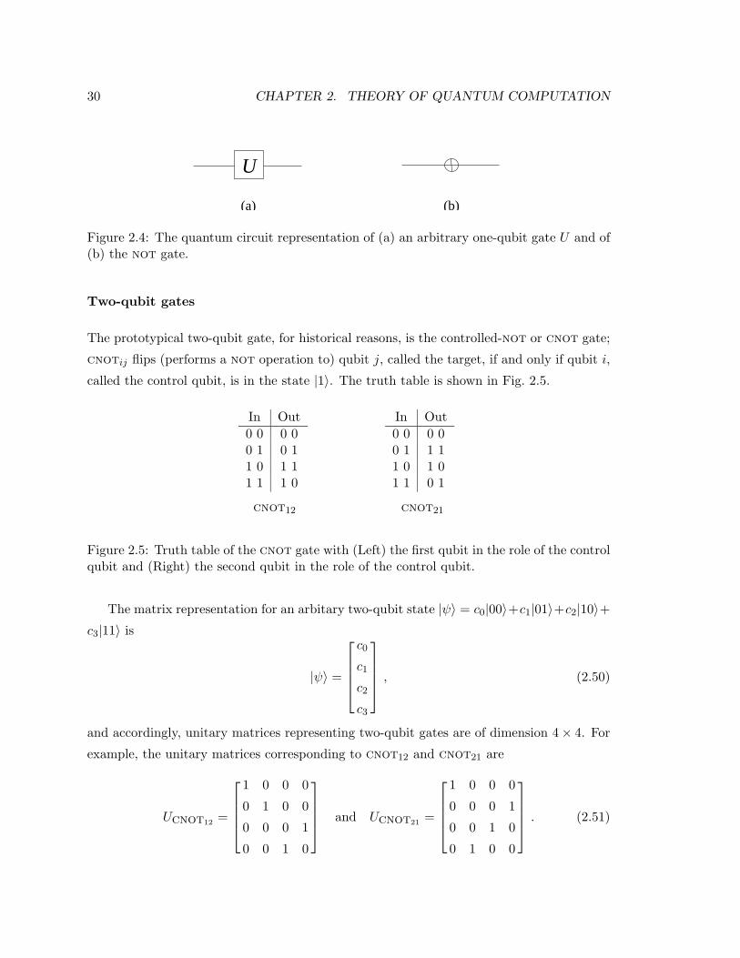
30 CHAPTER 2. THEORY OF QUANTUM COMPUTATION
U
(a) (b)
Figure 2.4: The quantum circuit representation of (a) an arbitrary one-qubit gate U and of(b) the not gate.
Two-qubit gates
The prototypical two-qubit gate, for historical reasons, is the controlled-not or cnot gate;
cnotij flips (performs a not operation to) qubit j, called the target, if and only if qubit i,
called the control qubit, is in the state |1〉. The truth table is shown in Fig. 2.5.
In Out0 0 0 00 1 0 11 0 1 11 1 1 0
In Out0 0 0 00 1 1 11 0 1 01 1 0 1
cnot12 cnot21
Figure 2.5: Truth table of the cnot gate with (Left) the first qubit in the role of the controlqubit and (Right) the second qubit in the role of the control qubit.
The matrix representation for an arbitary two-qubit state |ψ〉 = c0|00〉+c1|01〉+c2|10〉+c3|11〉 is
|ψ〉 =
c0
c1
c2
c3
, (2.50)
and accordingly, unitary matrices representing two-qubit gates are of dimension 4× 4. For
example, the unitary matrices corresponding to cnot12 and cnot21 are
Ucnot12 =
1 0 0 0
0 1 0 0
0 0 0 1
0 0 1 0
and Ucnot21 =
1 0 0 0
0 0 0 1
0 0 1 0
0 1 0 0
. (2.51)
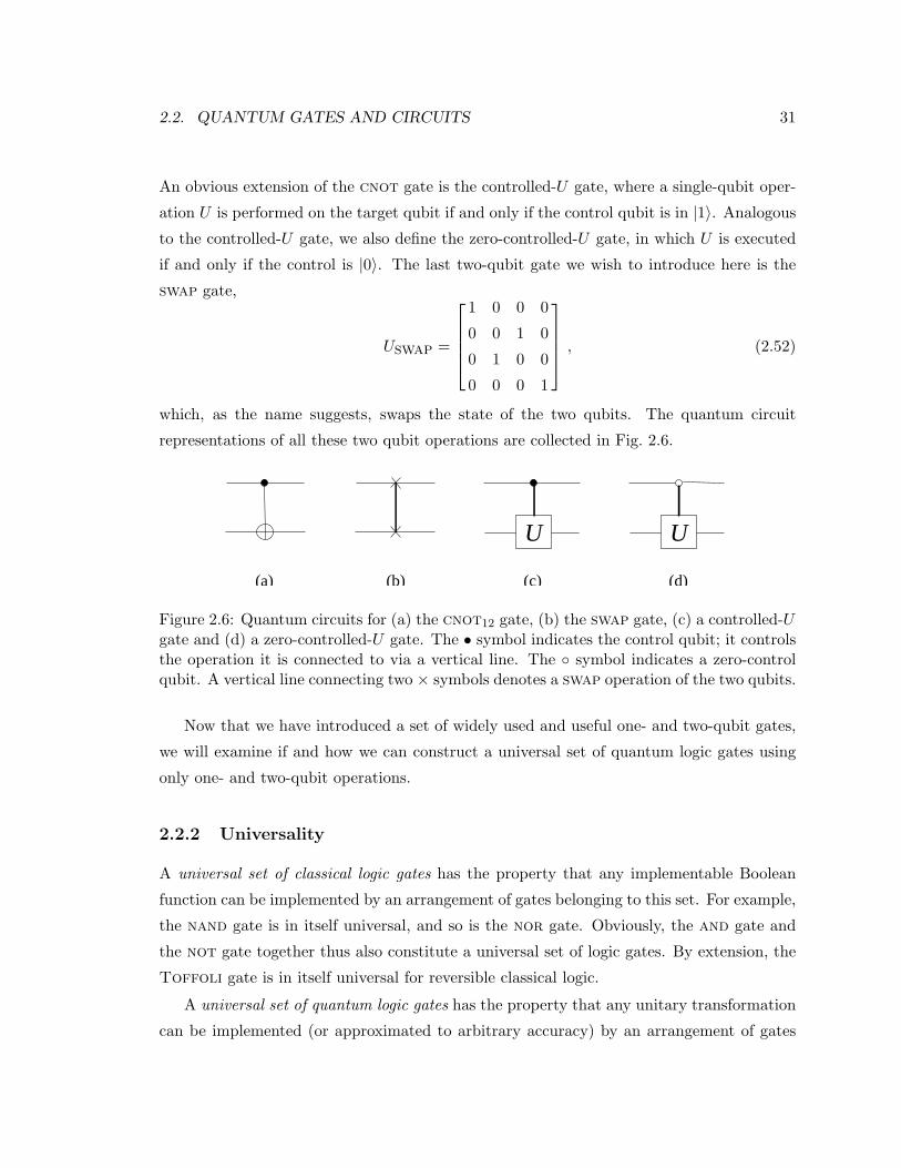
2.2. QUANTUM GATES AND CIRCUITS 31
An obvious extension of the cnot gate is the controlled-U gate, where a single-qubit oper-
ation U is performed on the target qubit if and only if the control qubit is in |1〉. Analogous
to the controlled-U gate, we also define the zero-controlled-U gate, in which U is executed
if and only if the control is |0〉. The last two-qubit gate we wish to introduce here is the
swap gate,
Uswap =
1 0 0 0
0 0 1 0
0 1 0 0
0 0 0 1
, (2.52)
which, as the name suggests, swaps the state of the two qubits. The quantum circuit
representations of all these two qubit operations are collected in Fig. 2.6.
(a) (b)
UU
(c) (d)
Figure 2.6: Quantum circuits for (a) the cnot12 gate, (b) the swap gate, (c) a controlled-Ugate and (d) a zero-controlled-U gate. The • symbol indicates the control qubit; it controlsthe operation it is connected to via a vertical line. The symbol indicates a zero-controlqubit. A vertical line connecting two × symbols denotes a swap operation of the two qubits.
Now that we have introduced a set of widely used and useful one- and two-qubit gates,
we will examine if and how we can construct a universal set of quantum logic gates using
only one- and two-qubit operations.
2.2.2 Universality
A universal set of classical logic gates has the property that any implementable Boolean
function can be implemented by an arrangement of gates belonging to this set. For example,
the nand gate is in itself universal, and so is the nor gate. Obviously, the and gate and
the not gate together thus also constitute a universal set of logic gates. By extension, the
Toffoli gate is in itself universal for reversible classical logic.
A universal set of quantum logic gates has the property that any unitary transformation
can be implemented (or approximated to arbitrary accuracy) by an arrangement of gates
32 CHAPTER 2. THEORY OF QUANTUM COMPUTATION
belonging to this set. Clearly, the Toffoli is not universal for quantum logic, as it is for
example not possible to create a superposition state starting from the ground state using
just Toffoli gates. Deutsch presented a three-qubit gate (a rotation of one qubit condi-
tioned upon two other qubits being |1〉) which is universal [Deu89]; DiVincenzo presented a
universal set of four two-qubit gates [DiV95b]. Lloyd [Llo95a] and independently Deutsch,
Barenco and Ekert [DBE95], extended this result to show that almost any two-qubit gate
is universal.
Of course, certain sets of universal quantum gates are more practical than others to
work with, and we will come back to this in section 3.1.2. The most widely used result in
the theory of quantum gates is that
the combination of the cnot gate with arbitrary single-qubit rotations constitutes
a set of universal quantum gates.
In fact, the cnot along with arbitrary rotations about x and y is sufficient as well, as
it can be shown that for any single-qubit rotation U there exist real numbers α, β, γ and δ
such that
U = eiαRx(β)Ry(γ)Rx(δ) . (2.53)
We will give examples of decompositions of multi-qubit gates into just single-qubit gates
and cnot’s in section 2.2.4.
We close by remarking that universality does not say anything about efficiency. In
fact, it has been proven that the required number of elementary operations, such as cnots
and single-qubit rotations, increases exponentially with n for almost all n-qubit unitary
operations. Therefore, a crucial part in the design of quantum algorithms is to prove that
each of the steps can be implemented efficiently, i.e. in only polynomially many elementary
operations.
2.2.3 Remarks on unitary operators
This section with technical remarks answers two questions: (1) how do we compute the
unitary operator corresponding to several consecutive gates, and (2) given an operation
which acts on a subset of n qubits, how do we write the 2n × 2n unitary matrix which
describes the evolution of the n qubits ?
2.2. QUANTUM GATES AND CIRCUITS 33
Multiplication and commutation of unitary operators
The concatenation of several quantum logic gates is described by the product of the corre-
sponding unitary matrices, ordered such that the operator of the first gate is placed on the
right. Thus, the unitary operator of k consecutive operations U1, U2, . . . , Uk is written as
U = UkUk−1 . . . U2U1 . (2.54)
This may seem awkward but makes sense if we recall Eq. 2.37, because this way U1 is
applied to |ψ〉 first, then U2 and so forth. The order is important since in general
U2U1 6= U1U2 , (2.55)
that is, in general, two unitary operators may not commute under multiplication. Her-
mitian matrices also may or may not commute with each other. Furthermore, for two
non-commuting Hermitian operators H1 and H2,
e−iH1e−iH2 6= e−iH2e−iH1 , (2.56)
e−iH1e−iH2 6= e−i(H1+H2) , (2.57)
e−iH2e−iH1 6= e−i(H1+H2) . (2.58)
These inequalities demonstrate the importance of commutation properties for quantum
computing. Turning on two terms in the Hamiltonian at the same time does not have the
same effect as turning them on one after the other; and turning on one first and then the
other is not the same as the other first and then the one. In closing, let us introduce a few
simple practical commutation rules:
1. Any unitary operator commutes with itself.
2. Unitary operators acting on different qubits commute.
3. All diagonal operators commute with each other.
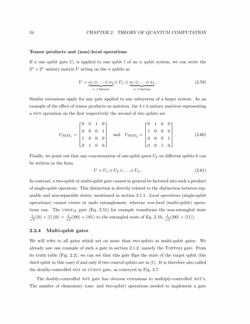
34 CHAPTER 2. THEORY OF QUANTUM COMPUTATION
Tensor products and (non)-local operations
If a one–qubit gate U1 is applied to one qubit l of an n qubit system, we can write the
2n × 2n unitary matrix U acting on the n qubits as
U = σI ⊗ . . .⊗ σI︸ ︷︷ ︸l−1 factors
⊗ U1 ⊗ σI ⊗ . . .⊗ σI︸ ︷︷ ︸n−l factors
, (2.59)
Similar extensions apply for any gate applied to any subsystem of a larger system. As an
example of the effect of tensor products on matrices, the 4×4 unitary matrices representing
a not operation on the first respectively the second of two qubits are
Unot1 =
0 0 1 0
0 0 0 1
1 0 0 0
0 1 0 0
and Unot2 =
0 1 0 0
1 0 0 0
0 0 0 1
0 0 1 0
. (2.60)
Finally, we point out that any concatenation of one-qubit gates Uk on different qubits k can
be written in the form
U = U1 ⊗ U2 ⊗ . . .⊗ Un . (2.61)
In contrast, a two-qubit or multi-qubit gate cannot in general be factored into such a product
of single-qubit operators. This distinction is directly related to the distinction between sep-
arable and non-separable states, mentioned in section 2.1.1. Local operations (single-qubit
operations) cannot create or undo entanglement, whereas non-local (multi-qubit) opera-
tions can. The cnot12 gate (Eq. 2.51) for example transforms the non-entangled state1√2(|0〉+ |1〉)|0〉 = 1√
2(|00〉+ |10〉) to the entangled state of Eq. 2.10, 1√
2(|00〉+ |11〉).
2.2.4 Multi-qubit gates
We will refer to all gates which act on more than two-qubits as multi-qubit gates. We
already saw one example of such a gate in section 2.1.2, namely the Toffoli gate. From
its truth table (Fig. 2.2), we can see that this gate flips the state of the target qubit (the
third qubit in this case) if and only if two control qubits are in |1〉. It is therefore also called
the doubly-controlled not or ccnot gate, as conveyed in Fig. 2.7.
The doubly-controlled not gate has obvious extensions to multiply-controlled not’s.
The number of elementary (one- and two-qubit) operations needed to implement a gate

2.3. QUANTUM ALGORITHMS 35
V V V
V =
√ i2
√−i2√
−i2
√i2
Figure 2.7: Quantum circuit representation of the Toffoli or ccnot gate, and its decom-position into two-qubit gates. We note that V 2 = Unot.
with n− 1 control qubits is O(n2). If we allow a scratch pad qubit (an ancilla), the number
of elementary operations is only O(n) [BBC+95].
Another useful and historically important gate is the Fredkin gate [FT82], or controlled-
swap gate, which swaps the state of two qubits if and only if a third qubit is in |1〉. The
two-qubit swap gate (see page 31) between qubits 2 and 3 can be implemented as cnot23
cnot32 cnot23, or by symmetry also as cnot32 cnot23 cnot32. Therefore, a possible
implementation of a swap of qubits 2 and 3 controlled by qubit 1 is as given in Fig. 2.8.
Figure 2.8: Quantum circuit representation of the Fredkin or cswap gate, and two quan-tum circuits equivalent to the Fredkin gate.
Efficient constructions for gates controlled by more than two qubits are extensively
described in the literature [BBC+95, DiV98]. In sections 5.9 and 5.10 respectively, we
will present quantum circuits for specific multi-qubit gates that were implemented in our
experiments.
2.3 Quantum algorithms
2.3.1 The Deutsch-Jozsa algorithm
In 1992, David Deutsch and Richard Jozsa invented the first ever quantum algorithm [DJ92].
The Deutsch-Jozsa algorithm achieves an exponential advantage over classical algorithms

36 CHAPTER 2. THEORY OF QUANTUM COMPUTATION
in solving Deutsch’s problem [DBE95] with certainty. Deutsch’s problem may be described
as follows. You are given a black box or oracle f which takes n input bits and returns one
output bit. Furthermore you are told that the black box either outputs the same value (0
or 1) for all possible input strings x, or outputs 0 for exactly half the possible input values
and 1 for the other input values. Deutsch’s problem is a thus a promise problem, and the
promise is that f is either constant or balanced.
How many oracle queries do you need classically to solve Deutsch’s problem with cer-
tainty ? As soon as you find that the oracle returns 0 for some inputs and 1 for other inputs,
you know for certain that f is balanced. However, if it the output is still the same after
trying 2n/2 different input values, the function f might still be balanced, even though most
likely it is constant. Only when 2n/2 + 1 input values produce the same output, you can
be sure the function is really constant. Thus, in the worst case, you need 2n/2 + 1 queries.
Using a quantum computer, the input of the oracle can be put in a superposition of all
possible input values, and a single oracle query suffices to determine with certainty whether
f is constant or balanced. We note that rather than to compute individual f(x), which we
know a quantum computer cannot do in fewer steps than a classical computer, the task is
to determine a global property of the function, namely whether f is constant or balanced.
This is a type of problem for which quantum computers may offer an advantage.
Procedure
The steps of the Deutsch-Jozsa algorithm, as improved by Cleve et al. [CEMM98] and
Tapp [Tap98], are outlined in Fig. 2.9. The initial state is
|ψ0〉 = |0〉⊗n|1〉 , (2.62)
where ⊗n indicates that the first register, the input register, is of size n (we will often leave
this impicit). The second register, the output register, contains only one qubit. First we
apply a hadamard gate on each of the n+ 1 qubits, resulting in the state
|ψ1〉 =2n−1∑x=0
|x〉√2n
[|0〉 − |1〉√
2
]. (2.63)
The input register is now in an equal superposition of all possible x. The reason why
the output register is placed in |0〉−|1〉√2
will become clear shortly. Next we query the oracle
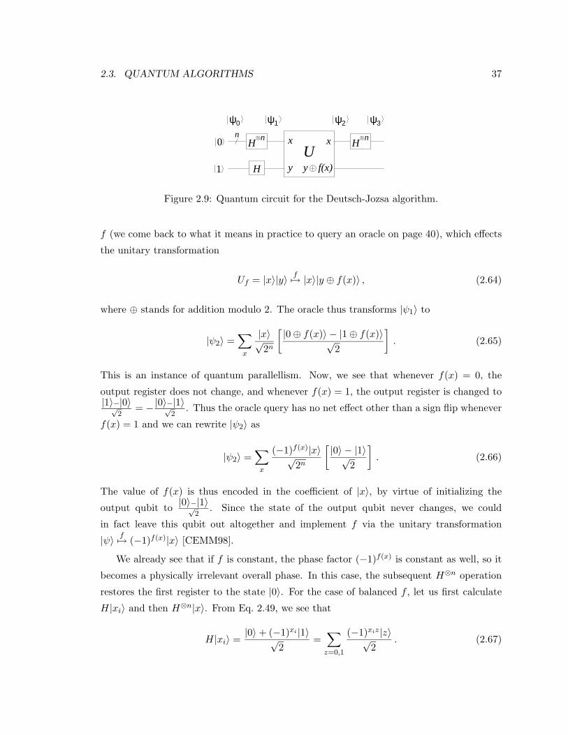
2.3. QUANTUM ALGORITHMS 37
0
ψ0
nH
nH
1 y y f(x)
n
ψ ψ ψ1 2 3
xxU
H
Figure 2.9: Quantum circuit for the Deutsch-Jozsa algorithm.
f (we come back to what it means in practice to query an oracle on page 40), which effects
the unitary transformation
Uf = |x〉|y〉 f7→ |x〉|y ⊕ f(x)〉 , (2.64)
where ⊕ stands for addition modulo 2. The oracle thus transforms |ψ1〉 to
|ψ2〉 =∑x
|x〉√2n
[|0⊕ f(x)〉 − |1⊕ f(x)〉√
2
]. (2.65)
This is an instance of quantum parallellism. Now, we see that whenever f(x) = 0, the
output register does not change, and whenever f(x) = 1, the output register is changed to|1〉−|0〉√
2= −|0〉−|1〉√
2. Thus the oracle query has no net effect other than a sign flip whenever
f(x) = 1 and we can rewrite |ψ2〉 as
|ψ2〉 =∑x
(−1)f(x)|x〉√2n
[|0〉 − |1〉√
2
]. (2.66)
The value of f(x) is thus encoded in the coefficient of |x〉, by virtue of initializing the
output qubit to |0〉−|1〉√2
. Since the state of the output qubit never changes, we could
in fact leave this qubit out altogether and implement f via the unitary transformation
|ψ〉 f7→ (−1)f(x)|x〉 [CEMM98].
We already see that if f is constant, the phase factor (−1)f(x) is constant as well, so it
becomes a physically irrelevant overall phase. In this case, the subsequent H⊗n operation
restores the first register to the state |0〉. For the case of balanced f , let us first calculate
H|xi〉 and then H⊗n|x〉. From Eq. 2.49, we see that
H|xi〉 =|0〉+ (−1)xi |1〉√
2=∑z=0,1
(−1)xiz|z〉√2
. (2.67)

38 CHAPTER 2. THEORY OF QUANTUM COMPUTATION
Therefore,
H⊗n|x1, . . . , xn〉 =
∑z1,...,zn
(−1)x1z1+...+xnzn |z1, . . . zn〉√2n
=∑
z(−1)x·z|z〉√2n
, (2.68)
where x ·z is the bitwise inner product of x and z, modulo 2. Using this result, we find that
|ψ3〉 = H⊗n|ψ2〉 =∑z
∑x
(−1)x·z+f(x)|z〉√2n
[|0〉 − |1〉√
2
]. (2.69)
We now measure the first register. For constant f , the amplitude of the |0〉⊗n term,∑x(−1)f(x), is either +1 or −1, depending on the constant value f takes. Given the
normalization condition of Eq. 2.9, the amplitude of the remaining terms must thus be
zero, like we anticipated. For balanced f , we always have that∑
x(−1)f(x) = 0 as there
are as many positive as negative f(x). The amplitude of the |0〉⊗n term is thus zero in
this case. In summary, if the measurement of the first register gives all 0’s we know f is
constant, and otherwise f is balanced.
Significance
We have thus shown that the Deutsch-Jozsa algorithm solves Deutsch’s problem exponen-
tially faster than any classical machine. While this is truly remarkable in itself, the practical
importance of this algorithm is limited. First, Deutsch’s problem is an artificial mathemat-
ical problem which has no known applications. Second, classical computers can solve this
problem quickly and with high probability of success by asking the oracle what f(x) is for a
few random x: the probability for obtaining k times the same answer (either 0 or 1) if f is
balanced decreases as (1/2)k−1. Only if absolute certainty is required, exponentially many
oracle queries may be required classically.
The significance of this algorithm therefore lies mostly in that it inspired later, more
useful algorithms, is relatively easily understood, and can be used as a simple test for
implementations of quantum computers. In section 5.3, we will present such an experiment
on a two-qubit NMR quantum computer.

2.3. QUANTUM ALGORITHMS 39
2.3.2 Grover’s algorithm
In 1996, Lov Grover invented a quantum algorithm for unstructured searches [Gro96, Gro97].
An example of a structured search is finding the phone number matching with a certain name
using a phone book with N alphabetically listed names. An example of an unstructured
search is to find the name matching with a certain phone number using the same phone
book. The time this takes goes up linearly with N : on average you will have to try
[N(N+1)/2−1]/N ≈ N/2 different names before you find the one with the desired number.
In contrast, using Grover’s algorithm, such a search can be accomplished in√N attempts.
Mathematically, we can describe this as the following promise problem. Given an oracle
which returns f(x) = 0 for all values of x except for a unique entry x = x0 for which f(x) = 1
(there is a unique name x0 in the phone book which has the desired phone number), find
the special element x0 in the least number of oracle queries.
As in the Deutsch-Jozsa algorithm, the oracle query takes the form of the transformation
Uf = |x〉|y〉 f7→ |x〉|x⊕ y〉 , (2.70)
where we will initialize the state of the output qubit |y〉 to |0〉−|1〉√2
. As we have seen in
section 2.3.1, the content of the output register in fact doesn’t change, and f(x) is encoded
in the sign of |x〉. We will therefore leave out the second register and from now on only
consider the effect of the oracle call on |x〉.
Procedure and performance
The steps in Grover’s algorithm for a search space of size N = 2n are:
(a) Initialize to |0〉⊗n.
(b) Apply H⊗n to obtain 1√N
∑N−1x=0 |x〉.
(c) Repeat the following subroutine, known as the Grover iteration, dπ√N/4e times:
1. Query the oracle Uf : |x〉 f7→ (−1)f(x)|x〉. This flips the phase of the |x0〉 term.
2. Apply H⊗n.
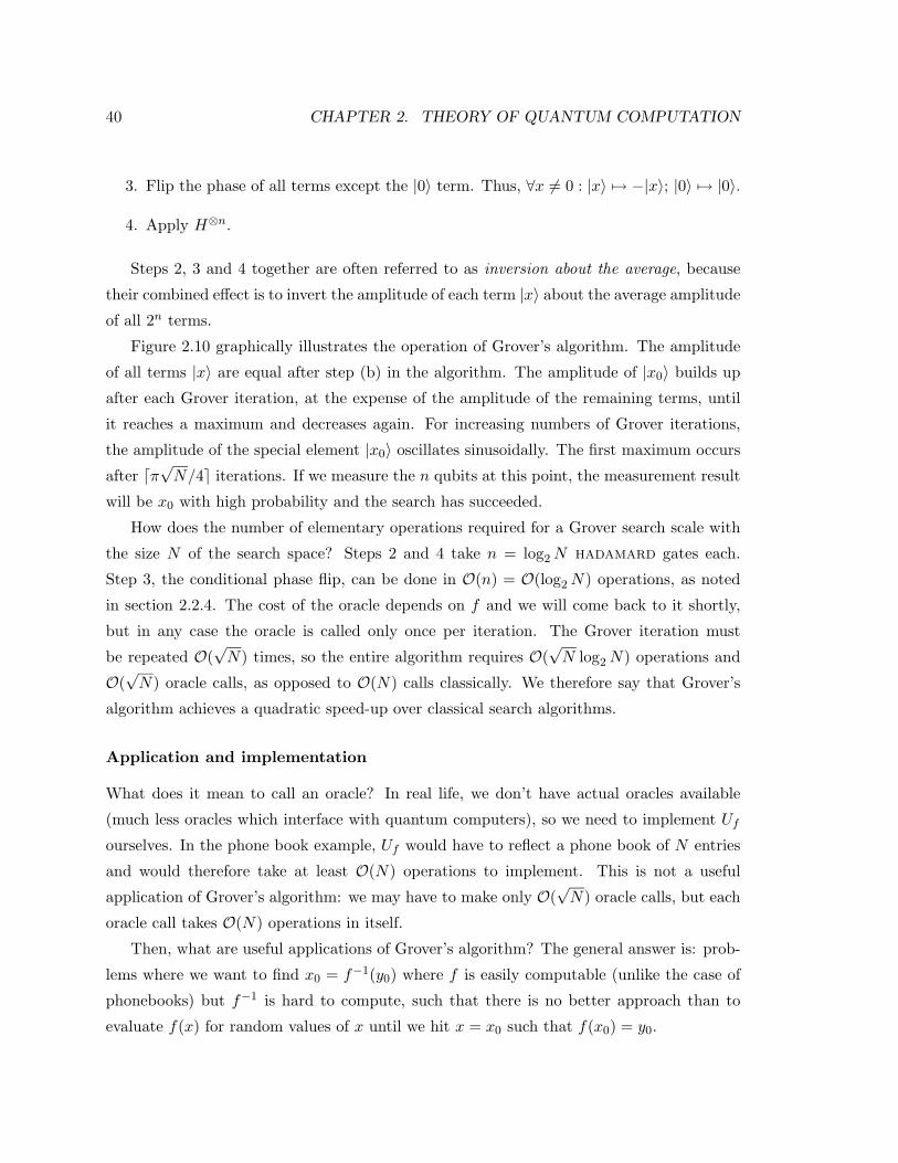
40 CHAPTER 2. THEORY OF QUANTUM COMPUTATION
3. Flip the phase of all terms except the |0〉 term. Thus, ∀x 6= 0 : |x〉 7→ −|x〉; |0〉 7→ |0〉.
4. Apply H⊗n.
Steps 2, 3 and 4 together are often referred to as inversion about the average, because
their combined effect is to invert the amplitude of each term |x〉 about the average amplitude
of all 2n terms.
Figure 2.10 graphically illustrates the operation of Grover’s algorithm. The amplitude
of all terms |x〉 are equal after step (b) in the algorithm. The amplitude of |x0〉 builds up
after each Grover iteration, at the expense of the amplitude of the remaining terms, until
it reaches a maximum and decreases again. For increasing numbers of Grover iterations,
the amplitude of the special element |x0〉 oscillates sinusoidally. The first maximum occurs
after dπ√N/4e iterations. If we measure the n qubits at this point, the measurement result
will be x0 with high probability and the search has succeeded.
How does the number of elementary operations required for a Grover search scale with
the size N of the search space? Steps 2 and 4 take n = log2N hadamard gates each.
Step 3, the conditional phase flip, can be done in O(n) = O(log2N) operations, as noted
in section 2.2.4. The cost of the oracle depends on f and we will come back to it shortly,
but in any case the oracle is called only once per iteration. The Grover iteration must
be repeated O(√N) times, so the entire algorithm requires O(
√N log2N) operations and
O(√N) oracle calls, as opposed to O(N) calls classically. We therefore say that Grover’s
algorithm achieves a quadratic speed-up over classical search algorithms.
Application and implementation
What does it mean to call an oracle? In real life, we don’t have actual oracles available
(much less oracles which interface with quantum computers), so we need to implement Ufourselves. In the phone book example, Uf would have to reflect a phone book of N entries
and would therefore take at least O(N) operations to implement. This is not a useful
application of Grover’s algorithm: we may have to make only O(√N) oracle calls, but each
oracle call takes O(N) operations in itself.
Then, what are useful applications of Grover’s algorithm? The general answer is: prob-
lems where we want to find x0 = f−1(y0) where f is easily computable (unlike the case of
phonebooks) but f−1 is hard to compute, such that there is no better approach than to
evaluate f(x) for random values of x until we hit x = x0 such that f(x0) = y0.
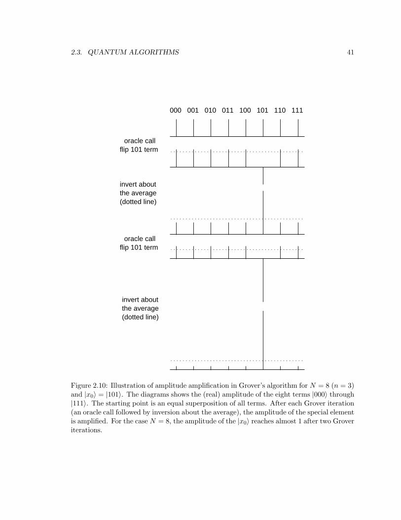
2.3. QUANTUM ALGORITHMS 41
invert aboutthe average(dotted line)
invert aboutthe average(dotted line)
000 001 010 011 100 101 110 111
flip 101 termoracle call
flip 101 termoracle call
Figure 2.10: Illustration of amplitude amplification in Grover’s algorithm for N = 8 (n = 3)and |x0〉 = |101〉. The diagrams shows the (real) amplitude of the eight terms |000〉 through|111〉. The starting point is an equal superposition of all terms. After each Grover iteration(an oracle call followed by inversion about the average), the amplitude of the special elementis amplified. For the case N = 8, the amplitude of the |x0〉 reaches almost 1 after two Groveriterations.

42 CHAPTER 2. THEORY OF QUANTUM COMPUTATION
As an example, consider the following instance of the satisfiability problem: find the
values of x1, x2 and x3 which satisfy the boolean expression (x1x2 + x3)x3. In this case,
it is easy to see that there is one unique solution, x1x2x3 = 100. However, the effort
needed to find a solution for an arbitrary Boolean expression, or even to ascertain whether
there is a solution, increases exponentially with the problem size for any known classical
algorithm. The general satisfiability problem is thus hard [Pap94] 5. A quantum computer
running Grover’s algorithm could solve this problem in quadratically fewer operations than
is possible classically.
For many realistic applications, such as the Satisfiability problem, there may be more
than one solution. However, if there are M solutions, the amplitude of the solutions is
highest after O(√N/M) Grover iterations [BBHT98]. We thus need to know M in order
to know the optimal number of iterations. Fortunately, M can be found in O(√N) oracle
calls as well, via a procedure called quantum counting [BHT98]. In summary, by combining
quantum counting and quantum search, unstructured searches with an unknown number of
solutions can be sped up quadratically compared to any classical algorithm.
In section 5.7, we will present an experimental realization of Grover’s algorithm on
a search space of eight elements. This experiment also nicely illustrates the oscillatory
behavior of the amplitude of |x0〉 as a function of the number of Grover iterations.
2.3.3 Order-finding and Shor’s algorithm
In 1994, Peter Shor discovered an efficient quantum algorithm for prime factorization and
for computing discrete logarithms [Sho94, Sho97]. This algorithm represented a tremen-
dous breakthrough, because it offered an exponential speed-up over both deterministic and
probabilistic classical algorithms for an important mathematical problem.
Shor’s algorithm was later generalized to an algorithm for order-finding and the Abelian
hidden-subgroup problem [Kit95]. The key step common to all algorithms in this class is the
quantum Fourier transform. We will first introduce the quantum Fourier transform (QFT),
then describe an algorithm which uses the QFT for order-finding, and finally present the
factoring algorithm as a specific instance of order-finding. For a good introductory article
on Shor’s algorithm, see [EJ96].
5A restricted case of the satisfiability problem, 2-sat, is not hard.

2.3. QUANTUM ALGORITHMS 43
The quantum Fourier transform
The quantum Fourier transform (QFT) performs the same transformation as the (classical)
fast Fourier transform (FFT), but it can be computed efficiently, which is classically not
possible. Or more precisely, the QFT allows us to efficiently sample the FFT. Even this
is impossible classically and, as we will see, being able to sample the FFT is sufficient for
order-finding.
The FFTN takes as input a string of N complex numbers xj and produces as output
another string of N complex numbers yk, such that
yk =1√N
N−1∑j=0
xje2πijk/N . (2.71)
For an input string with numbers which repeat themselves with period r, the FFTN inverts
the periodicity, i.e. it produces an output string with period N/r, as illustrated in the
following four examples for N = 8 (the output strings have been rescaled for clarity)
r input string output string N/r
8 1 0 0 0 0 0 0 0 7→ 1 1 1 1 1 1 1 1 1 (2.72)
4 1 0 0 0 1 0 0 0 7→ 1 0 1 0 1 0 1 0 2 (2.73)
2 1 0 1 0 1 0 1 0 7→ 1 0 0 0 1 0 0 0 4 (2.74)
1 1 1 1 1 1 1 1 1 7→ 1 0 0 0 0 0 0 0 8 (2.75)
If r does not divide N , the inversion of the period is approximate. In addition to
inverting the period, the FFT converts off-sets in the locations of the numbers in the input
string into phase factors in front of the numbers in the output string:
1 0 0 0 1 0 0 0 7→ 1 0 1 0 1 0 1 0 (2.76)
0 1 0 0 0 1 0 0 7→ 1 0 −i 0 −1 0 i 0 (2.77)
0 0 1 0 0 0 1 0 7→ 1 0 −1 0 1 0 −1 0 (2.78)
0 0 0 1 0 0 0 1 7→ 1 0 i 0 −1 0 −i 0 (2.79)
The QFT performs exactly the same transformation, but differs from the FFT in that

44 CHAPTER 2. THEORY OF QUANTUM COMPUTATION
the complex numbers are stored in the amplitude and phase of the terms in a superposition
state of n = log2N qubits. For N = 8, the qubit string is of length log2 8 = 3, and
the amplitude of the |000〉 term represents the first complex number, the amplitude of the
|001〉 term represents the second number and so forth. As before, we will label the states
|000〉, |001〉, . . . |111〉 as |0〉, |1〉, . . . |7〉. As an example, we see from Eq. 2.77 that the QFT
thus transforms the state |1〉+ |5〉 to the state |0〉 − i|2〉 − |4〉+ i|6〉.The action of the QFT on a computational basis state of length n is
|j〉 7→ 1√N
N−1∑k=0
e2πijk/N |k〉 , (2.80)
which we can rewrite (after some algebra) as
|j1, . . . , jn〉 7→(|0〉+ e2πi0.jn |1〉)(|0〉+ e2πi0.jn−1jn |1〉) · · · (|0〉+ e2πi0.j1j2···jn |1〉)√
2n, (2.81)
where 0.j1j2 . . . jn stands for 2−j1 + 2−2j2 + . . .+ 2−njn . Suppose we now reverse the order
of the qubits in the output of the QFT, so output qubit jn becomes output qubit 1, qubit
jn−1 becomes qubit j2 and so forth. The transformation of Eq. 2.81 then changes into
|j1, . . . , jn〉 7→(|0〉+ e2πi0.j1 |1〉)(|0〉+ e2πi0.j2j1 |1〉) · · · (|0〉+ e2πi0.jnjn−1···j1 |1〉)√
2n. (2.82)
which we can easily implement as follows. The first factor of this expression represents a
180 phase shift of qubit 1 controlled by qubit 1 itself; this is accomplished by a hadamard
gate on qubit 1. The next factor shifts the phase of qubit 2 over 180 controlled by qubit 2 (a
hadamard gate on qubit 2), and over another 90 controlled by qubit 1, which corresponds
to a controlled-Z rotation. The next factor requires a hadamard gate on qubit 3, a Z
rotation of qubit 3 controlled by qubit 2 and a Z1/2 (45) rotation of 3 controlled by 1. The
quantum circuit for the QFT acting on three qubits is shown in Fig. 2.11, and it can be easily
extended for n > 3, using a total of n hadamard gates and n(n−1)/2 controlled rotations.
We next see how the QFT is incorporated in a quantum algorithm for order-finding.
Order-finding
The order of a permutation π on M = 2m elements can be understood via the following
analogy: imagine M rooms and M one-way passages connecting the rooms, with exactly

2.3. QUANTUM ALGORITHMS 45
j3
j
j2
1
j
j2
3
1jHH
H
90
45 90
Figure 2.11: Quantum circuit for the quantum Fourier transform (QFT) acting on threequbits. In this implementation of the QFT, due to Coppersmith [Cop94], the order of thequbits is reversed at the output with respect to the input.
one entrance and one exit in each room (for some rooms, the passage going out may loop
back to the room itself). The rooms are thus connected in subcycles, as shown in Fig. 2.12.
This configuration ensures that if you start in some room y and keep going from one room
to the next using the one-way passages, you must eventually come back to the room you
started from. We then define the order r of the permutation π as the minimum number of
transitions needed to return to the starting room y, where r may depend on y but is never
greater than M .
5 3
4
6 0
1
7
2
Figure 2.12: Pictorial representation of a permutation π on eight elements. The order r is3 if y ∈ 2, 4, 5, r = 1 if y = 6, and r = 4 if y ∈ 0, 1, 3, 7.
Suppose you are in a room y and must determine the order r solely by making trials
of the type “make x transitions starting from room y and check which room you are in”.
Mathematically, we will describe such trials as queries of an oracle or black box which
outputs πx(y), that is the element obtained after permuting x times starting from y using
π (so for the permutation of Fig. 2.12, we have π1(5) = 4, π2(5) = 2 and so forth). How
many such queries are needed in order to find r with a given probability of success ?
Richard Cleve [Cle00] showed that the minimum number of classical oracle queries
needed for a given probability of success increases exponentially with the problem size
m (m = log2M is the number of bits needed to represent M numbers). In contrast, on
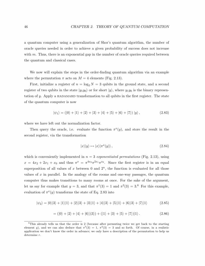
46 CHAPTER 2. THEORY OF QUANTUM COMPUTATION
a quantum computer using a generalization of Shor’s quantum algorithm, the number of
oracle queries needed in order to achieve a given probability of success does not increase
with m. Thus, there is an exponential gap in the number of oracle queries required between
the quantum and classical cases.
We now will explain the steps in the order-finding quantum algorithm via an example
where the permutation π acts on M = 4 elements (Fig. 2.13).
First, initialize a register of n = log2N = 3 qubits in the ground state, and a second
register of two qubits in the state |y1y0〉 or for short |y〉, where y1y0 is the binary represen-
tation of y. Apply a hadamard transformation to all qubits in the first register. The state
of the quantum computer is now
|ψ1〉 = (|0〉+ |1〉+ |2〉+ |3〉+ |4〉+ |5〉+ |6〉+ |7〉) |y〉 , (2.83)
where we have left out the normalization factor.
Then query the oracle, i.e. evaluate the function πx(y), and store the result in the
second register, via the transformation
|x〉|y〉 7→ |x〉|πx(y)〉 , (2.84)
which is conveniently implemented in n = 3 exponentiated permutations (Fig. 2.13), using
x = 4x2 + 2x1 + x0 and thus πx = π4x2π2x1πx0 . Since the first register is in an equal
superposition of all values of x between 0 and 2n, the function is evaluated for all those
values of x in parallel. In the analogy of the rooms and one-way passages, the quantum
computer thus makes transitions to many rooms at once. For the sake of the argument,
let us say for example that y = 3, and that π1(3) = 1 and π2(3) = 3.6 For this example,
evaluation of πx(y) transforms the state of Eq. 2.83 into
|ψ2〉 = |0〉|3〉+ |1〉|1〉+ |2〉|3〉+ |3〉|1〉+ |4〉|3〉+ |5〉|1〉+ |6〉|3〉+ |7〉|1〉 (2.85)
= (|0〉+ |2〉+ |4〉+ |6〉)|3〉) + (|1〉+ |3〉+ |5〉+ |7〉)|1〉 . (2.86)
6This already tells us that the order is 2 (because after permuting twice we get back to the startingelement y), and we can also deduce that π3(3) = 1, π4(3) = 3 and so forth. Of course, in a realisticapplication we don’t know the order in advance; we only have a description of the permutation to help usdetermine r.
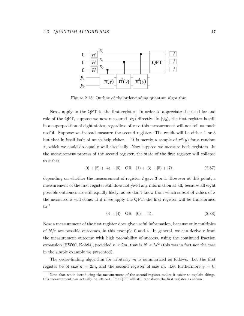
2.3. QUANTUM ALGORITHMS 47
H
H
H2x
x1
x0
( )yπ
0
0
0
π ( )y4π ( )y2
QFT
1
0
y
y
Figure 2.13: Outline of the order-finding quantum algorithm.
Next, apply to the QFT to the first register. In order to appreciate the need for and
role of the QFT, suppose we now measured |ψ2〉 directly. In |ψ2〉, the first register is still
in a superposition of eight states, regardless of π so this measurement will not tell us much
useful. Suppose we instead measure the second register. The result will be either 1 or 3
but that in itself isn’t of much help either — it is merely a sample of πx(y) for a random
x, which we could do equally well classically. Now suppose we measure both registers. In
the measurement process of the second register, the state of the first register will collapse
to either
|0〉+ |2〉+ |4〉+ |6〉 OR |1〉+ |3〉+ |5〉+ |7〉 . (2.87)
depending on whether the measurement of register 2 gave 3 or 1. However at this point, a
measurement of the first register still does not yield any information at all, because all eight
possible outcomes are still equally likely, as we don’t know from which subset of values of x
the measured x will come. But if we apply the QFT, the first register will be transformed
to 7
|0〉+ |4〉 OR |0〉 − |4〉 . (2.88)
Now a measurement of the first register does give useful information, because only multiples
of N/r are possible outcomes, in this example 0 and 4. In general, we can derive r from
the measurement outcome with high probability of success, using the continued fraction
expansion [HW60, Kob94], provided n ≥ 2m, that is N ≥M2 (this was in fact not the case
in the simple example we presented).
The order-finding algorithm for arbitrary m is summarized as follows. Let the first
register be of size n = 2m, and the second register of size m. Let furthermore y = 0,
7Note that while introducing the measurement of the second register makes it easier to explain things,this measurement can actually be left out. The QFT will still transform the first register as shown.

48 CHAPTER 2. THEORY OF QUANTUM COMPUTATION
without loss of generality.
1. Initialize
|0〉|0〉
2. Create a superposition using H⊗n
7→ 1√2n
2n−1∑j=0
|j〉|0〉
3. Apply f(j) (where f(j) = πj(0))
7→ 1√2n
2n−1∑j=0
|j〉|f(j)〉
4. Apply the QFTN to the first register (Eq. 2.80)
7→ 12n
2n−1∑j=0
2n−1∑k=0
e2πijk/N |k〉|f(j)〉
=12n
2n−1∑k=0
2n−1∑j=0
e2πijk/N |k〉|f(j)〉
5. Measure the first register
The probability for obtaining |k〉 upon measurement is the square of the amplitude of
|k〉 in the output state of the QFT,
2n−1∑j=0
e2πijk/N
2
. (2.89)
Due to interference of the terms in this summation, the probability is high for values of k
which are an integer multiple of N/r and very small or zero for other values of k. In fact,
if r divides N exactly, the probability for obtaining a multiple of N/r upon measuring the
output state is equal to 1 (this was the case in the examples for the FFT of Eqs. 2.72-2.75).
In section 5.9, we will present the first implementation of the order-finding algorithm.

2.3. QUANTUM ALGORITHMS 49
We will next describe a specific instance of the order-finding algorithm, namely Shor’s
famous algorithm for prime factorization.
Factoring
The most famous application of the order-finding algorithm, and historically the first one
to be discovered, is to decompose larger integer numbers into their prime factors. Quantum
factoring consists of finding the order of the permutation
π(y) = ay modL , (2.90)
for y = 1. L is the integer we want to factor and a can be any integer < L that is
coprime with L (i.e. a and L should have no common factors other than 1). In words, the
permutation consists of multiplying y by a, and taking the remainder of the division of ay
by L.
Given the order r of the permutation ay modL for y = 1, at least one prime factor of L
is given by
gcd(ar/2 − 1, L) or gcd(ar/2 + 1, L) (2.91)
with high probability. Computing the greatest common denominator of two integers can be
done efficiently on a classical computer, using Euclid’s algorithm. These are results from
number theory [HW60, Kob94].
An important difference between our description of the order-finding problem and the
factoring problem is that for order-finding we assumed that an oracle was available which
we can ask queries of the type πx(y). As was pointed out in section 2.3.2, we must in
practice implement oracle calls ourselves, and we must therefore consider whether this can
be done efficiently. For factoring, calling the oracle means implementing the permutation
πx(y) = axy modL with y = 1, which is equivalent to evaluation of the function
ax modL , (2.92)
known as the modular exponentiation function.
Since ax modL is by definition a number between 0 and L− 1, the second register must
be of size m = dlog2 Le. The first register must be at least twice as large, so n = 2m. Since
50 CHAPTER 2. THEORY OF QUANTUM COMPUTATION
x = xn−12n−1 + . . .+ x121 + x020, we have
axy modL = a2n−1xn−1 . . . a2x1 ax0y modL
= [a2n−1xn−1 . . . [a2x2 [ax0y modL] modL] . . .modL] (2.93)
In words, this means that we first multiply y by a modulo L, if and only if x0 = 1; then
we multiply the result by a2 modulo L, if and only if x1 = 1 and so forth, until we finally
multiply by a2n−1modulo L if and only if xn−1 = 1.
Thus, modular exponentiation is reduced to n = 2m ≈ 2 log2 L multiplications modulo
L, each controlled by just a single qubit xi. The numbers a2, . . . , a2n−1mod L by which we
need to multiply can be found efficiently on a classical computer by repeated squaring, and
multiplication of m-bit numbers take O(m2) elementary operations.
The modular exponentiation step can thus be done efficiently, in O((log2 L)3) one- and
two-qubit gates, and we showed earlier that the other key step in Shor’s factoring algorithm,
the quantum Fourier transform, can also be realized efficiently. The factoring problem,
widely believed to be intractable on classical computers, 8 is thus tractable on quantum
computers.
In section 5.10, we present the first experimental realization of Shor’s algorithm. It is an
implementation of the simplest possible instance for which the algorithm can be non-trivially
demonstrated, namely factorization of the number fifteen 9.
2.3.4 Quantum simulations
The possibility of using quantum computers to solve problems in quantum physics was
was conjectured by Feynman [Fey82] long before quantum algorithms for solving mathe-
matical problems such as factoring were discovered. Seth Lloyd proved this conjecture in
1996 [Llo96].
The general procedure is to map the possible states of the simulated system onto the
states of a set of qubits, and then to apply a sequence of quantum gates which produce
8We note that classically, there are many approaches known to factoring integers besides finding theorder of ay modN , but all of them are inefficient. It is possible, although unlikely, that one day an efficientclassical factoring algorithm will be found. Or perhaps a proof will be constructed that such an algorithmis not possible.
9The algorithm fails for even L and for L which are powers of prime numbers (e.g. the number nine),and factoring is obviously not applicable to prime L. This includes all numbers smaller than 15. The nextsimplest instance of factoring is 21
2.3. QUANTUM ALGORITHMS 51
qubit dynamics analogous to the dynamics of the simulated system. The final state of the
qubits is then mapped back onto the state of the simulated system.
Explicit protocols have been worked out for several realistic physical problems. These
include
• Estimation of the eigenvalues and eigenvectors of a Hamiltonian (this algorithm in-
vokes the QFT), which can be used to find the energy levels of an atom for exam-
ple [AL99].
• Simulation of the dynamics of many-body Fermi systems, using either first or second
quantized descriptions [AL97].
• Simulation of quantum chaos and localization [GS01].
2.3.5 Other quantum algorithms and perspectives
The three main classes of quantum algorithms are (1) those based on the quantum Fourier
transform, (2) search algorithms, and (3) quantum simulations. All of these were invented
in the mid-nineties. Since then, the range of applications of these algorithms has been
extended and refined. However, virtually no fundamentally new algorithms for quantum
computers have been discovered, despite intense effort all over the world.
It would be disappointing if no other applications were found than those currently
known. Nevertheless, existing algorithms are already of significant practical interest. In
particular, quantum simulations may address a broad range of physics problems which
are otherwise intractable. For example, as transistors and other devices continue to shrink,
simulation of their operation at the quantum level may be crucially important but impossible
to do on classical computers.
The impact of quantum computing on the fundamentals of computer science may be just
as profound and long-lasting, as it appears that the strong Church-Turing thesis must be
revised. This thesis states that any two universal Turing machines (a general computational
device [Tur36]) are polynomially equivalent; in other words, the Church-Turing thesis says
that problems which can be efficiently computed on one Turing machine can always be
efficiently computed on another Turing machine. However, quantum Turing machines,
proposed by David Deutsch [Deu85], appear to be capable of efficiently solving problems
which are intractable on classical Turing machines.

52 CHAPTER 2. THEORY OF QUANTUM COMPUTATION
2.4 Quantum error correction
Quantum computers, like any machine, may have faulty or unreliable components. In order
to nevertheless perform reliable computations, errors in the state of the qubits must be
corrected.
Quantum error correction is similar to its classical analogue in many respects. Input
states are encoded in a larger system which is more robust against noise or other error
processes than unencoded states, in the sense that the original information can be retrieved
with greater likelyhood if the input states are encoded than if they are not.
For example, a simple classical code encodes 0 as 000 and encodes 1 as 111. If we send
an uncoded bit of information through a noisy channel which flips a bit with probability p,
then the probability of error per use of the channel is also p. However, if we send the same
bit of information in encoded form (three physical bits), and take a majority vote between
the three bits after the noise process, we can correctly guess the bit of information unless
two of the physical bits are flipped, which happens with probability 3(1− p)p2, or all three
physical bits are flipped, which occurs with probability p3. The resulting probability of
error per bit of information is thus only 3p2 − 2p3, which is smaller than p if 0 < p < 1/2.
Classically, encoding can thus decrease the error probability at the expense of using extra
bits and encoding/decoding operations.
We would like to use similar schemes to encode quantum information, in order to pro-
tect quantum computers and quantum communication channels against errors caused by
decoherence. However, quantum error correction is much more tricky than classical error
correction, because
1. it is not possible to build up redundancy by simply making copies of the quantum
state, due to the no-cloning theorem [Die82, WZ82].
2. measurement of a quantum system destroys its state, so it is not possible to check the
state of a qubit,
3. quantum errors can be arbitrary rotations in the Bloch sphere, while in classical
computers only bit flips (0↔ 1) can occur.
The remarkable and surprising achievement of Shor [Sho95] and Steane [Ste96] was to
show that it is nevertheless possible to reverse the truly random errors due to decoherence.
The underlying principles are
2.4. QUANTUM ERROR CORRECTION 53
1. to use entanglement in order to realize a quantum analogue of redundancy,
2. to measure errors without measuring the quantum state itself,
3. to digitize the errors (force an arbitrary error to collapse into either no error or a full
bit flip, a phase flip or a bit-and-phase flip).
There are many excellent references on the theory of quantum error correction [EM96,
KL96]. We here describe in detail a two-qubit error detection code, which nicely illustrates
how the three guiding principles of quantum error correction are put into practice. Next,
we give a brief overview of larger codes, capable of detecting and correcting more errors,
and introduce the notion of fault-tolerancy.
2.4.1 The two-qubit phase error detection code
The two-qubit phase error detection code [CL95] encodes one qubit information in the joint
state of two qubits. After decoding, it is possible to tell whether or not a phase error
occurred on one of the qubits. If an error is detected, the state is rejected; otherwise it is
kept.
The two-qubit phase error detection code encodes logical 0 and 1 as
|0L〉 =1√2
(|00〉+ |11〉) (2.94)
|1L〉 =1√2
(|01〉+ |10〉) , (2.95)
where the subscript L denotes logical states. An arbitrary qubit state a|0〉+ b|1〉 is encoded
as
|ψ3〉 = a|0L〉+ b|1L〉 (2.96)
=1√2
[a(|00〉+ |11〉) + b(|01〉+ |10〉)
], (2.97)
via the quantum circuit of Fig. 2.14. We thus build up redundancy by encoding the logical
qubit in the state of two qubits using entanglement (principle 1).
Now let us first consider an error process which causes a complete phase flip of one or
more qubits, where we define a phase flip of qubit i as σiz ρ σiz. For a code to detect errors,
it suffices that all errors to be detected map the codeword space C (the space spanned by

54 CHAPTER 2. THEORY OF QUANTUM COMPUTATION
Figure 2.14: Encoding and decoding quantum circuit for the two-qubit code. In betweenencoding and decoding, phase damping may disturb the qubit states.
|0L〉 and |1L〉) onto its orthogonal complement. In this way, detection of errors can be done
unambiguously by a projection onto C without distinguishing individual codewords, hence
without disturbing the encoded information (principle 2). This is precisely what the code
of Eq. 2.95 achieves.
The four possible outcomes of the error process are
|ψII〉 = I ⊗ I |ψ〉 = a|00〉+ |11〉√
2+ b|01〉+ |10〉√
2(2.98)
|ψZI〉 = σz ⊗ I |ψ〉 = a|00〉 − |11〉√
2+ b|01〉 − |10〉√
2(2.99)
|ψIZ〉 = I ⊗ σz|ψ〉 = a|00〉 − |11〉√
2+ b−|01〉+ |10〉√
2(2.100)
|ψZZ〉 = σz ⊗ σz|ψ〉 = a|00〉+ |11〉√
2+ b−|01〉 − |10〉√
2, (2.101)
with the erroneous states |ψZI〉 and |ψIZ〉 orthogonal to the correct state |ψII〉. After
decoding, which is the inverse of the encoding operation (see Fig. 2.14):
|ψII〉dec⇒ (a|0〉+ b|1〉)|0〉 (2.102)
|ψZI〉 ⇒ (a|0〉 − b|1〉)|1〉 (2.103)
|ψIZ〉 ⇒ (a|0〉+ b|1〉)|1〉 (2.104)
|ψZZ〉 ⇒ (a|0〉 − b|1〉)|0〉 . (2.105)
We note that the ancilla (the auxiliary qubit) becomes |1〉 upon decoding if and only
if a single phase error has occurred. Furthermore, the two qubits are in a product state
2.4. QUANTUM ERROR CORRECTION 55
after decoding, so it is possible to read out the syndrome (which indicates whether or not
a phase error occurred) by a projective measurement on the ancilla without measuring the
encoded state, which is held in the first qubit. If the final state of the ancilla is |0〉, we trust
the state of the first qubit is properly preserved, and accept it. If the ancilla is in |1〉, we
distrust the state of the first qubit and reject it.
Clearly, the error σz ⊗ σz cannot be detected, but this occurs only with probability p2,
where we let p be the probability that the phase of a qubit is flipped in the error process.
Furthermore, the code can detect phase errors but cannot reveal which qubit has the error,
so it cannot correct errors. Moreover, |ψIZ〉 decodes to a correct state in the first qubit
which is rejected. This affects the absolute fidelity (the overall probability of successful
recovery) but not the conditional fidelity (the probability of successful recovery if the state
is accepted). All of these properties are intrinsic limitations of using an error detection
code as opposed to an error correction code. With only two physical qubits per qubit of
information, an error detection code is the best we can do.
So far we have considered only complete phase flip errors, but in reality phase shifts
over arbitrary angles may occur. Fortunately, we can discretize such errors (principle 3)
as follows. Suppose the error is an arbitrary phase shift on the first qubit: |0〉 → |0〉,|1〉 → eiθ|1〉. Then, the encoded state becomes
1√2
[a(|00〉+ eiθ|11〉) + b(eiθ|10〉+ |01〉)
](2.106)
=1√2
1 + eiθ
2
[a(|00〉+ |11〉) + b(|10〉+ |01〉)
]+
1√2
1− eiθ
2
[a(|00〉 − |11〉) + b(−|10〉+ |01〉)
]. (2.107)
The decoded state is now a superposition of the states given by Eqs.(2.102) and (2.103):
1√2
1 + eiθ
2(a|0〉+ b|1〉)|0〉+
1√2
1− eiθ
2(a|0〉 − b|1〉)|1〉 . (2.108)
Measurement of the second qubit projects it to either |0〉 or |1〉. Because of entanglement,
the first qubit is projected accordingly to having no phase error, or a complete phase flip!
An arbitrary phase shift of the second qubit is discretized in the same manner.
In section 5.4, we will present an NMR demonstration of the operation of the two-qubit
phase error detection code.

56 CHAPTER 2. THEORY OF QUANTUM COMPUTATION
2.4.2 Error correction codes and fault-tolerancy
Codes with more than two physical qubits per logical qubit are capable not only of detecting
errors but also of correcting errors. Historically, the first two quantum codes capable of
correcting arbitrary single-qubit errors were a nine-qubit code [Ste96] and a seven-qubit
code [Sho95]. A five-qubit code followed later [LMPZ96].
Using counting arguments based on the (quantum) Hamming bound, we can see that
five is the minimum number of qubits that can be used to correct arbitrary errors. A code
which encodes one logical qubit in k physical qubits has k − 1 ancillae which can represent
up to 2k−1 orthogonal error syndromes. There are three types of errors which can occur
on each of the physical qubits: a phase flip, a bit flip and a combined phase and bit flip
(those can be expressed mathematically as σx, σz and σy errors respectively). It is also
possible that no error occurs on any of the k qubits. Thus, assuming that the errors acting
on different qubits are uncorrelated, we need 3k + 1 orthogonal error syndromes, to be
represented by the 2k−1 ancillae. This way, we can simply measure the ancilla qubits upon
decoding, infer precisely what error occurred and on which qubit it acted, and then correct
the error. The requirement for the length k of the codewords is therefore that
2k−1 ≥ 3k + 1 . (2.109)
If only one type of error is expected to occur, say phase errors, Eq. 2.109 can be relaxed to
2k−1 ≥ k + 1, and a three-qubit code is sufficient. Also, analogous to the case of classical
codes, more efficient codes can be constructed by encoding several logical qubits per code-
word.
Implicit in our discussion of quantum error correction so far is the assumption that the
encoding and decoding operations are perfect, and that the qubits are simply sent through
a noisy channel. In the context of quantum computation, such a channel would correspond
to a quantum memory device. However, in realistic quantum computers, information must
also be protected in the course of a computation, and furthermore encoding and decoding
operations are themselves subject to errors. Would it still be helpful to apply quantum
error correction under these circumstances?
The surprising answer is yes, provided the decoherence rate is below a certain level, the
accuracy threshold, expressed as the probability of error per elementary logic operation on
2.5. SUMMARY 57
one or two qubits [ABO97, Kit97, KLZ98].
This notion is developed in the theory of fault-tolerant quantum computation [Got98].
Using concatenated quantum codes and quantum circuits which minimize error propagation
between qubits, the net error rate can be made arbitrarily small, provided the “raw” error
rate is below the accuracy threshold. Thus, a reliable quantum computer can be constructed
from unreliable components.
2.5 Summary
The combination of fundamental concepts in quantum physics, computer science and infor-
mation theory have led to the rich field of quantum computation. Three main theoretical
results of this field are that
1. the complexity of quantum systems grows exponentially with the number of elemen-
tary quantum systems involved,
2. certain problems which appear intractable on any classical computer are tractable on
a quantum computer,
3. reliable quantum computers can be constructed from unreliable components, provided
the error rate is below the accuracy threshold.
These results highlight the theoretical potential of quantum computation for fundamen-
tally new systems and devices, capable of reliably solving problems beyond the reach of
classical machines. From the presentation in this chapter, requirements for the implemen-
tation of quantum computers naturally emerge. This is the subject of the next chapter.
Chapter 3
Implementation of quantum
computers
In the first half of this chapter, we ask ourselves what the fundamental requirements are
for building a quantum computer. In the second half, we briefly review the state of the art
in various proposed embodiments of quantum computers.
3.1 Requirements
Our understanding of the minimal requirements for quantum computation has grown con-
siderably over the years. They are often formulated as the five criteria of David DiVin-
cenzo [DiV00]. These are
1. a scalable physical system with well characterized qubits
2. a universal set of quantum gates,
3. the ability to initialize the state of the qubits to a simple fiducial state, such as
|00 . . . 0〉,
4. a qubit-specific measurement capability,
5. long relevant decoherence times, much longer than the gate operation time.
We shall now explore each of these criteria in detail, in order to develop a good under-
standing of their significance as well as their stringency.
58

3.1. REQUIREMENTS 59
3.1.1 Qubits
The heart of a quantum computer is a set of physical systems which represent the state
of the quantum bits. Since a qubit is by definition a two-level quantum system, spin-1/2
particles and polarized photons are natural realizations of qubits. In practice, a qubit may
also be represented by two levels of a large manifold of levels, for example two energy levels
of an atom. Proposed qubit embodiments range from trapped atoms and ions to nuclear
and electron spins, electric charge, magnetic flux and photons (see section 3.2).
Size of the qubit register
The complexity of just a 40-qubit quantum computer far exceeds the complexity of most
classical computers. That is, a classical computer would need vastly more time to simulate
the dynamics of a 40 qubit computer than it would take the quantum computer itself to
run, even if the clock speed of the classical computer is much greater than the clock speed
of the quantum computer, because the quantum computer can explore 240 computational
paths in parallel.
However, in order to factor a 400 digit number (a task well beyond the capability of
classical computers for the foreseeable future), a few thousand logical qubits are required.1
With error correction, 10 to 100 times more qubits would be needed.
Fortunately, some other interesting applications require much more moderate numbers
of qubits. For example, a quantum computer with 50 to 100 qubits (not counting a possible
overhead for error correction) could compute the electronic orbitals of a small atom such as
boron with greater accuracy than any classical simulation performed to date [AL99].
Alternatives to qubits
In principle, a three-level (or higher) quantum system could also serve as the basic unit
of quantum information. However, this offers no computational advantage and all current
proposals for the physical implementation of quantum computers are based on qubits.
Could we use one 2n level system instead of n two-level systems? Both have a 2n
dimensional Hilbert space and are mathematically perfectly equivalent. However, in a 2n
level system, the levels must either extend over an exponentially large range of energies or1The second register in the order-finding algorithm must be large enough to represent the integer to be
factored, which would be log2 10400 = 400 log2 10 ≈ 1329 bits, and the first register must be at least twiceas large as the second register. In practice, additional scratchpad qubits may be desired.
60 CHAPTER 3. IMPLEMENTATION OF QUANTUM COMPUTERS
must lie exponentially close together. Clearly, this is not a scalable approach to quantum
computing.
Finally, could we use continuous variables, such as the position or momentum of a
particle, to represent quantum information? Properties such as entanglement of continuous
variables have been explored both theoretically and experimentally [BK98]. However, the
precision of any physical device is limited by noise, and it thus appears always necessary for
a realistic computer to discretize the continuous variables in order to perform computations
[LB99].
3.1.2 Quantum gates
The time evolution of a closed quantum system is determined by its Hamiltonian (sec-
tion 2.1.2). In order to realize quantum logic gates, we must therefore be able to control the
Hamiltonian over time such that the resulting time evolutions correspond to the computa-
tional steps of an algorithm [Ben80]. A tremendously helpful theoretical result is that there
exist small sets of unitary transformations which are universal for quantum computation
(section 2.2.2). We shall here single out one particular universal set of gates, the combina-
tion of arbitrary single-qubit rotations with the cnot gate, which has also been the set of
choice in the literature. The starting point for our discussion of quantum gates is that we
require
the ability to manipulate the Hamiltonian accurately, quickly and selectively such that
we can perform a universal set of one- and two-qubit gates on individual qubits or pairs of
qubits.
Coupling network
We must be able to perform two-qubit gates between any two qubits in a quantum computer.
However, a computer with pairwise couplings between all the qubits (Fig. 3.1 a) is nearly
impossible to build, as interactions between physical particles tend to rapidly decrease with
the separation between the particles. For example, nuclear spins in a molecule are well
coupled if they are united in a chemical bond, but the couplings are weaker or sometimes
zero for two- and three-bond couplings.

3.1. REQUIREMENTS 61
A common architecture in proposed quantum computer realizations uses only nearest-
neighbour couplings between qubits placed in a linear or two-dimensional array (Fig. 3.1 b).
This is the case for many solid-state proposals, such as inductively coupled SQUID loops,
quantum dots connected by tunneling barriers and nuclear spins of donor atoms, coupled
via the overlap between the respective electron clouds.
Fortunately, we can effect two-qubit gates between any pair of qubits even if they aren’t
all directly coupled to each other, as long as there exists a path of couplings that indirectly
connects any two qubits. For example, in order to perform a cnot13 gate with the coupling
network of Fig. 3.1 (b), we can first swap the state of qubits 1 and 2 (this can be done via
the sequence cnot12 cnot21 cnot12), then perform a cnot23, and finally swap qubits 1
and 2 again. The net effect is a cnot13.
1 2
35
4
1 2 3 4 5
1 2 3 4 5(a)
(b)
(c)
BUS
Figure 3.1: Three extreme coupling networks between five qubits. (a) A full couplingnetwork. (b) A nearest-neighbour coupling network. (c) Coupling via a bus.
Even if none of the qubits are directly coupled to each other, it is still possible to
perform universal computation provided an external (but still quantum mechanical) degree
of freedom can be selectively coupled to any one qubit in a controlled manner (Fig. 3.1 c).
The external degree of freedom serves as a bus and can facilitate two-qubit gates between
any pair of qubits in much the same way intermediary qubits can facilitate two-qubit gates
between any two qubits in Fig. 3.1.
Examples of such bus degrees of freedom are the collective motional state of an array
of trapped ions, a photon inside an optical cavity which holds several trapped atoms or
a photon which couples to several quantum dots embedded in a semiconductor structure.
Typically, the spatial range over which collective degrees of freedom can extend while main-
taining the ability to significantly couple to the qubits, is also limited. Therefore, such

62 CHAPTER 3. IMPLEMENTATION OF QUANTUM COMPUTERS
architectures may have to be supplemented by additional means for interactions between
different groups of qubits.
Time-dependent control over the Hamiltonian
It is not always necessary that we can turn on and off all the terms in the Hamiltonian at will,
as long as we can reverse undesired time evolutions at a later stage. This is commonly done
for example in NMR, by so-called refocusing techniques (similar to spin-echoes), where the
ωσz term in the Hamiltonion cannot be switched off but it is possible to perform a Rx(180)
or not gate. By applying the not gate halfway a time interval t and again at the end, the
ωσz evolution which took place in the first time interval is unwound in the second interval,
so there is no net evolution (up to an overall and thus irrelevant phase shift). We can verify
this mathematically using Eqs. 2.41, 2.42, 2.45 and 2.47:
Rx(180)e−iωσzt/2Rx(180)e−iωσzt/2 =
(−iσx) [cos(ωt/4)σI − i sin(ωt/4)σz] (−iσx) [cos(ωt/4)σI − i sin(ωt/4)σz] = −σI (3.1)
for any t. The same refocusing technique can be used to time-reverse evolution under the
Hamiltonian σizσjz, as also
σix exp(−itσizσjz/2) σix exp(−itσizσjz/2) = −σiIσjI , (3.2)
for any t. This is pictorially illustrated for the case of NMR in Fig. 4.11. Of course, it isn’t
always so easy to reverse undesired evolutions, as we will see for example in section 4.2, but
nevertheless the use of unitary operations to time-reverse specific undesired evolutions can
tremendously reduce the fabrication requirements for quantum computers.
Selective addressability
We have started from the assumption that we must be able to selectively perform one- and
two-qubit logic gates on arbitrary qubits. However, we can circumvent the need for selective
control of single- and two-particle Hamiltonians by storing each logical qubit in the state of
three physical qubits.
Seth Lloyd showed that universal quantum computation is possible using a cellular

3.1. REQUIREMENTS 63
automata 2 architecture of the form
D −ABC −ABC − ...−ABC
where the different physical qubits A cannot be distinguished from each other nor selectively
addressed, and likewise for the B’s and C’s [Llo93]. Each unit cell ABC is used to represent
one qubit. In the default situation, the qubits of information are stored in the physical qubits
B, and the A’s and C’s are set to 0, except in one unit cell i, where A is set to 1.
A single-qubit operation U on qubit i and qubit i only is obtained via a controlled-U
operation of A on B when Ai is set to 1 while the Aj (j 6= i) are set to 0. By applying
cnot gates on the whole array, we can move up or down the index of the unique A which
is marked as 1. A controlled-U operation of qubit i onto qubit i − 1 can be realized using
cnots and a doubly-controlled U gate for which Ai (set to 1) acts as one of the control
qubits. The special site D is needed to load the initial state. The same site D can be used
to read out the answer to the computation one bit at a time.
This model is reasonably well approximated by nuclear spins in long polymers. It may
also ease the fabrication requirements for many solid-state proposals, including electron
spins in quantum dots, nuclear spins in donor atoms, or nuclear spins in a crystal.
Universality without single-qubit terms in the Hamiltonian
Single-qubit operations are not strictly necessary for universal quantum computation; in
fact, it has been shown that “almost any” two-qubit gate is universal [DBE95, Llo95a]. Un-
fortunately, virtually none of these universal two-qubit gates can be generated by naturally
occurring two-particle Hamiltonians. The underlying reason is that most interaction Hamil-
tonians provided by nature exhibit too much symmetry in the two qubits. The exchange
Hamiltonian,
H = ~σ1 · ~σ2 = σ1xσ
2x + σ1
yσ2y + σ1
zσ2z , (3.3)
which describes the interaction between electron spins in quantum dots coupled through a
tunneling barrier (and related proposals), is an example of such a symmetrical two-qubit
Hamiltonian.
2Computer scientists actually use this term to describe an even more stringent computational model,where the same operation is applied over and over on all the bits in the computer. Surprisingly, even such astringent model can be used to perform meaningful (classical) computations.
64 CHAPTER 3. IMPLEMENTATION OF QUANTUM COMPUTERS
However, by encoding each logical qubit in the state of three physical qubits, univer-
sal quantum computation is nevertheless possible [DBLW00]. The physical qubits must
be placed in a linear array and it must be possible to selectively switch on and off the
interactions between neighbouring physical qubits (by tweaking the tunneling barrier in
the example). State initialization to an encoded basis state is accomplished by cooling the
system down to its ground state in the presence of select couplings.
Encoding each logical qubit in the state of two physical qubits is also possible but
only if the two physical qubits have a different effective magnetic moment [Lev01]. The
two encoded basis states are |01〉 and |10〉; they are clearly susceptible to the exchange
interaction. An additional advantage is that fewer operations are needed.
Universality without two-qubit terms in the Hamiltonian
Quantum computation appears to inherently require non-linear interactions, i.e. two-qubit
terms in the Hamiltonian, in order to realize two-qubit gates. However, universal quan-
tum computation is possible with only linear (i.e. single-qubit) quantum gate elements,
supplemented by measurements and classical feedback, which provide the needed non-
linearity [KLM01] and allow one to create entangled qubits via a probabilistic scenario.
Using the entanglement thus created, two-qubit gates are accomplished by a clever combi-
nation of teleportation and single-qubit gates [GC99].
This proposal has been developed in the context of optical realizations of quantum com-
puters, where it is difficult to obtain appreciable non-linear interactions between quantum
bits (photons) without too much absorption. Potentially, the scheme may be translated
into other physical systems.
Accuracy and speed
An obvious requirement is that the quantum gates be executed with high fidelity, i.e. that
the resulting unitary transformation be as close as possible to the desired unitary evolution.
If that is not possible, we must have sufficient information over the actual evolution and
sufficient control over the Hamiltonian such that we can undo erroneous evolutions at a
later point in time.
Erroneous unitary evolutions that cannot be unwound, have the same detrimental effect
on the computation as random errors due to decoherence and thus effectively increase the
decoherence rate. While they can still be corrected using quantum error correction, this is

3.1. REQUIREMENTS 65
associated with a large overhead. Furthermore, quantum error correction is only effective
if the total error rate (due to decoherence and erroneous unitary evolutions combined) is
below the accuracy threshold, introduced in section 2.4.2.
In order to achieve the accuracy threshold, the duration of a typical logic operation τopmust be short compared to the coherence time τc. Obviously, the speed and accuracy of
logic gates do usually not go hand in hand, so it is key to make an optimal trade-off.
Finally, whereas the clock speed is irrelevant from a complexity theory point of view —
only the scaling of the number of operations with the problem size is relevant —, a quantum
computer with a clock speed of 20 Hz (a realistic number for solution NMR for example) may
appear to be of little practical use. However, let us say that factoring a 400 digit number
would take two hundred thousand quantum operations, which is a reasonable estimate,
and further that quantum error correction would increase this number by a factor of one
hundred. The resulting twenty million operations would take a “lousy” 20 Hz quantum
processor one million seconds, which is not even 12 days, still quite fast given that the same
problem would classically take even the fastest supercomputer longer than the age of the
universe to solve.
3.1.3 Initialization
A fundamental condition for computation which is often taken for granted is the ability to
reliably prepare a known input state. If the input state of a computation is random, the
output is of little use 3. Thus, we demand
the ability to reliably prepare a pure input state.
We recall from section 2.1.1, page 13 that the term “pure” implies that the state is
known. If all we know about a qubit is that it is in one of several states |ψi〉, with certain
probabilities, then the qubit is said to be in a statistical mixture of states, as opposed to a
pure state.
Unlike for the case of classical computers where it is usually easy to reset or initialize bits,
state initialization can be very difficult in quantum computers, depending on the physical3Classically, the output for a random input value may sometimes be of interest, for example if the task
is to determine whether a certain output value occurs at all. However, since quantum computations arereversible, the output is always a permutation of the input, and therefore the output for a random inputholds no information at all.

66 CHAPTER 3. IMPLEMENTATION OF QUANTUM COMPUTERS
realization of the qubits. In qubit implementations where the |0〉 and |1〉 states have distinct
energies, we can prepare the qubits in their ground state by letting them equilibrate at a
low enough temperature T such that the energy difference ∆E between the ground and
excited states satisfies the condition
∆E kBT , (3.4)
where kB is Boltzmann’s constant. Otherwise, the thermally equilibrated qubits are in
a statistical mixture of states, described by the density matrix ρeq = exp(−H/kBT )/Z,
where Z is a normalization factor. At room temperature, kBT ≈ 26 meV, which is much
larger than realistic values of ∆E for many quantum systems. Therefore, many proposed
realizations of quantum computers require cryogenic temperatures, often in the 10 or 100
mK range.
We note that the ability to perform a hard measurement (introduced on page 20 and
further discussed in section 3.1.4), automatically leads to the ability to prepare a pure input
state: it suffices to measure the qubit’s state, and change it if needed.
Unfortunately, in many proposed realizations of quantum computers, it is impossible or
very difficult to set up the qubits in a pure initial state. However, might it not be possible
to access the computational power of quantum systems as long as the state of the qubits is
not completely random (ρ 6= I/2n) ?
Effective pure states
Remarkably, it is indeed possible to perform arbitrary quantum computations on a mixed
state, provided the mixed state is effective pure, or pseudo-pure and the observables are
traceless [GC97, CPH98] (see section 3.1.4). Effective pure states are mixed states described
by a density matrix of the form
ρeff =1− α
2nI + α |ψ〉〈ψ| . (3.5)
For traceless observables, the identity component I does not produce any signal at all.
Furthermore, I doesn’t evolve under unitary transformations, as UIU † = I for all unitary
operations U . A system in an effective pure state ρeff thus has the same dynamical be-
havior and produces the same signal (up to a proportionality factor α) as a system in the
corresponding pure state |ψ〉.

3.1. REQUIREMENTS 67
It is crucial that α not decrease exponentially with the number of qubits n, as α is directly
proportional to the signal strength. If it did, the precision of the measurement would have
to increase exponentially with n or the signal would have to be averaged over exponentially
many experiments. Such an exponential cost would obviously offset the exponential benefit
of quantum computers.
Several methods are known for the preparation of effective pure states starting from a
state in thermal equilibrium at high temperatures, all of which have been developed in the
context of liquid state NMR quantum computation. Unfortunately, all these methods have
in common that α ∝ n/2n. Then, is such an exponential overhead inevitably associated
with the use of high temperature qubits?
Cooling down a subset of hot qubits
The truly surprising answer is no: there exists a scalable algorithm for obtaining k pure
qubits starting from n partly mixed qubits. This algorithm, invented by Schulman and
Vazirani [SV99], has only a linear overhead in the number of qubits (k ∝ n) and a quasi-
linear, O(k log k), overhead in the number of operations. A related algorithm was devised
earlier by Cleve and DiVincenzo in the context of Schumacher compression; this algorithm
requires O(k3) operations and O(√k) zero entropy auxiliary qubits (which are recovered
at the end of the procedure). The Schulman-Vazirani algorithm, in contrast, is capable of
bootstrapping in the sense that it can create bits with (near) zero entropy starting from
only high entropy bits.
The idea behind the Schulman-Vazirani scheme is to redistribute the entropy over the
qubits, such that the entropy of a subset of the qubits approaches zero while the entropy
of the remaining qubits increases (the total entropy is preserved). In order to calculate
the maximum possible k as a function of n, let us define the polarization ε of a qubit as
the difference in probabilities between the ground and excited state, tracing out any other
qubits. Mathematically, the polarization of spin i is defined as
ε = Tr(ρσiz) . (3.6)
A qubit is thus in |0〉 with probability 1+ε2 and in |1〉 with probability 1−ε
2 . The theoretical
maximum kmax of zero temperature (ε = 1) bits that can be extracted from n bits with

68 CHAPTER 3. IMPLEMENTATION OF QUANTUM COMPUTERS
initial polarization ε0 is given by entropy conservation,
nH(
1+ε02
)= kH(1) + (n− k)H(1/2) , (3.7)
where the entropy H is given by
H(p) = −p log2 p− (1− p) log2(1− p) , (3.8)
so H(1) = H(0) = 0 and H(1/2) = 1. From Eq. 3.7, we find
kmax =[1−H
(1 + ε0
2
)]n , (3.9)
which for small ε0 is well approximated by
kmax ≈ ε20 n . (3.10)
Schulman and Vazirani showed that their scheme is not only efficient (the overhead is only
polynomial in n) but is also optimal, in that it achieves the entropic bound in the limit of
large n.
We will present an NMR implementation of the elementary building block of the Schulman-
Vazirani scheme in section 5.8, and describe the operation of this building block when we
discuss state initialization in NMR quantum computation (section 4.4.6).
3.1.4 Read-out
A computation can only be useful if we can access the final result. In a quantum com-
puter, the final result is represented by the final state of one or more qubits. We recall
(section 2.1.3, page 19) that it is not possible to obtain full information about unknown
qubit states, but also (section 2.3) that projective measurements in the |0〉, |1〉 basis are
sufficient if we use quantum algorithms. Furthermore, a different measurement basis is fine
too, since we can always change basis via a unitary transformation just before the measure-
ment. In summary, we need
the ability to perform accurate projective measurements of the qubit states.

3.1. REQUIREMENTS 69
Strong and weak measurements
Read-out of the state of a quantum system requires some form of coupling of the quantum
system to a classical measuring device, such that at the end of the measurement process, the
meter indicates the state of the quantum system, projected onto the measurement basis.
For example, measurement of the state of a qubit represented by two energy levels (|0〉and |1〉) in an atom can be done by pumping the |1〉 state and looking for fluorescence. If
the qubit was in |1〉, the atom will fluoresce, a stream of electrons will flow in a nearby
photomultiplier tube, and a signal will appear on the display of an electrometer. If the
atom was in |0〉, the electrometer will show no signal. If the qubit state was a|0〉+ b|1〉, the
measurement process will collapse the state into |0〉 or |1〉 and the observer will either see
a signal or see no signal, with probabilities |a|2 and |b|2.
Clearly, if the coupling with the measuring apparatus is so strong that the qubit states
instantaneously collapse — a scenario known as a hard or strong measurement — we must be
able to switch off the measuring device during the computation. However, it is also possible
to never switch off the measurement provided the quantum system is only weakly coupled
to the meter. In this scenario, called a weak measurement, information only very slowly
leaks out of the quantum system. On the one hand, the qubits therefore decohere only very
gradually, as opposed to instantaneously 4, but on the other hand, a weak measurement
implies that we cannot learn much about the state of the qubit.
Weak measurements therefore require the use of signal averaging, either over a large
ensemble of identical computers or over time-sequential experiments performed on a single
computer. Signal averaging may also be needed to boost the reliability of the measurement
if the detector efficiency and/or accuracy is limited.
Averaged measurements
Averaging the result of quantum computations poses a specific difficulty. For example, we
recall that in the order-finding algorithm (section 2.3.3), the measurement will with high
probability return an integer multiple of N/r, but we don’t know which multiple. From
any multiple lN/r, we can determine r with high probability of success via a classical com-
putation called the continued fraction expansion. A time averaged measurement, however,
gives ≈∑r
l=0 lN/r = 〈l〉N/r, and an ensemble averaged measurement gives 〈ln〉 . . . 〈l1〉N/r4Weak and strong measurements are understood as taking place on a timescale much slower or faster
than the duration of the computation.
70 CHAPTER 3. IMPLEMENTATION OF QUANTUM COMPUTERS
(where the 〈li〉 are the bitwise averages of l). Either way, it is not possible to compute r
from the averaged measurement outcome except in a few special cases.
This problem can be circumvented by calculating the continued fraction expansion on
the quantum computer without first measuring the output state of the order-finding quan-
tum algorithm [GC97]. Since the output of the continued fraction expansion is deterministic
(it is r), a time or ensemble averaged measurement of the qubits after the continued fraction
expansion will always give r as well. For all the known quantum algorithms with proba-
bilistic outputs, we can use similar derandomization procedures which permit the use of
averaged measurements.
Other remarks
• Do we have to be able to read out each individual physical qubit (the implicit assumption
so far)? The answer is no. It is sufficient to be able to measure the state of just one physical
qubit: at the end of the computation, we can swap one after the other logical qubit into
that physical qubit and measure it. Note that it would not be good to measure one qubit,
then repeat the computation and measure the next qubit, and so forth (unless the out-
put is derandomized [GC97]). Again taking order-finding as an example, we see that at the
end of each experiment, the one bit may come from to a different multiple of N/r every time.
• Do we need to be able to measure qubits during the computation? Again, the answer is
no. If no subsequent operations depend on the measurement outcome, such measurements
can be left out altogether. If subsequent operations on the remaining qubits do depend on
the measurement outcome, we can use controlled quantum gates instead.
• Does it matter if a measurement destroys the physical qubit that was measured? Here
also, the answer is no. In fact, after we measure a qubit, we can do almost anything we
want to it, including throw it away, because this will not affect the state of the remaining
qubits. However, interactions between the measured qubits and the remaining qubits must
be avoided or neutralized, because such interactions would alter the state of the remaining
qubits.

3.1. REQUIREMENTS 71
3.1.5 Coherence
The final requirement is that the qubits have a sufficiently long coherence time τc such that
quantum mechanical superposition states can be preserved throughout the execution of a
quantum algorithm (section 2.1.5). Or alternatively, and more realistically given the large
number of qubits and operations involved in realistic computations,
The decoherence rate must lie below the threshold error rate for fault-tolerant quantum
computation 5:
τop/τc < 10−4 , (3.11)
where τop is the typical duration of a quantum gate. Obviously, this is only a crude measure,
as τop covers a wide range of logic gates and τc lumps together a broad range of errors due to
a variety of decoherence processes and systematic errors which somehow cannot be reversed.
Mathematically, the effect of decoherence can be conveniently described in the operator-
sum representation
ρ 7→∑k
= EkρE†k . (3.12)
where the Ek are operators acting on the Hilbert space of the system. The interpretation
of this expression is that ρ is transformed to
EkρE†k
Tr(EkρE†k)
(3.13)
with probability
p(k) = Tr(EkρE†k) . (3.14)
For trace-preserving processes, the operators Ek must satisfy the completeness relation
∑k
E†kEk = I . (3.15)
The operator sum representation encompasses all physical processes which can act on a
quantum system, including non-unitary processes. We point out that any given physical
process has many possible operator sum representations, and can thus also be interpreted in5The estimated values for the accurracy threshold depend on the error model and on the architecture
of the quantum computer (e.g. whether or not there are only nearest-neighbour interactions between thequbits and whether or not parallel operations are allowed). Most estimates lie in the range of 10−6 to 10−4.

72 CHAPTER 3. IMPLEMENTATION OF QUANTUM COMPUTERS
different ways. We also note that for unitary processes, there is only one term in Eq. 3.12,
E0 = U .
The general rule for obtaining long coherence times is that the qubits be highly isolated
from the environment, because interactions with the environment and information leakage
to the environment are the cause of decoherence [Zur82, Zur91]. We will now review several
ways in which decoherence can manifest itself.
Energy dissipation
Energy dissipation is a decoherence process caused by the exchange of energy between a
quantum system and the environment (the bath). Physical examples of this process are
spontaneous emission in atoms or semiconductor structures, nuclear or electron spins which
return to the thermal equilibrium with the environment, heating of the motional state of
trapped ions, and so forth.
Energy dissipation to a bath at zero temperature is described by
ρ 7→ E0ρE†0 + E1ρE
†1 , (3.16)
where
E0 =[ 1 0
0√
1− γ
], E1 =
[ 0√γ
0 0
]. (3.17)
The E0 operation preserves a qubit in the ground state |0〉 but attenuates the excited state
|1〉; the E1 operation changes the |1〉 state into the |0〉 state with probability γ. The overall
result of this process, known as amplitude damping, is that a qubit in the excited state
decays into the ground state with probability γ, thereby loosing a quantum of energy to
the environment. As a result, an arbitrary one-qubit density matrix is transformed as[a b∗
b c
]7→[ 1− (1− γ)(1− a) b
√1− γ
b∗√
1− γ c(1− γ)
]. (3.18)
If the environment is at finite temperature, the process of Eq. 3.16 must be generalized
to
ρ 7→3∑
k=0
EkρE†k , (3.19)
3.1. REQUIREMENTS 73
where
E0 =√p
[ 1 0
0√
1− γ
], E1 =
√p
[ 0√γ
0 0
],
E2 =√
1− p[√1− γ 0
0 1
], E3 =
√1− p
[ 0 0√γ 0
]. (3.20)
Thus, a qubit in the excited state decays to the ground state with probability γp, and a qubit
in the ground state is lifted to the excited state with probability γ(1− p). The parameter p
depends on the temperature of the environment and the energy difference between |0〉 and
|1〉. The stationary state of this process, called generalized amplitude damping, is the mixed
state
ρ∞ =[p 0
0 1− p
]. (3.21)
We can geometrically visualize the effect of generalized amplitude damping via the trans-
formation of an arbitrary vector on the surface of the Bloch sphere
(rx, ry, rz) 7→(rx√
1− γ, ry√
1− γ, rz(1− γ) + γ(2p− 1)). (3.22)
In many physical systems, γ is a time-varying function of the form γ = 1− e−t/T1 , where T1
is a characteristic time constant, which was first introduced in NMR [Blo46]. It corresponds
to the lifetime of excited states. In real physical system, non-unitary exchange of energy can
also take place between different qubits in the system. This random process also represents
a form of decoherence, just like energy exchange between qubits and the bath.
Finally, we point out that in most proposed quantum bit implementations, energy dissi-
pation on the one hand adversely affects quantum computations, but on the other hand also
represents a natural mechanism for state initialization. After waiting for a sufficiently long
time (several times the T1), the qubits approach thermal equilibrium with the environment.
The thermal equilibrium state thus constitutes a reproducible and fiducial initial state. If
the environment is close enough to zero Kelvin such that ∆E kBT , the thermal equilib-
rium state is very close to being pure. For qubits in equilibrium with a high temperature
bath, additional state preparation operations must be performed in order to distill pure
qubits (section 3.1.3).

74 CHAPTER 3. IMPLEMENTATION OF QUANTUM COMPUTERS
Phase randomization
Phase randomization results in the loss of coherence (the phase relationship) between dif-
ferent basis states, and can caused by interactions with the environment. For example,
local fluctuations in the magnetic field randomize the phase of nuclear or electron spins;
and scattering with defects randomly disturbs the phase of free electrons in solids. In many
systems, phase randomization is the dominant decoherence process and the coherence time
τc is therefore often loosely taken to be the characteristic phase randomization time.
A phase shift over some random angle θ changes an arbitrary pure one-qubit state
|ψ〉 = a|0〉 + b|1〉 into Rz(θ)|ψ〉 = ae−iθ/2|0〉 + beiθ/2|1〉 (see Eq. 2.47). The density matrix
changes accordingly:
ρ = |ψ〉〈ψ| =
[|a|2 ab∗
a∗b |b|2
]7→ Rz(θ)ρRz(θ)† =
[|a|2 ab∗e−iθ
a∗beiθ |b|2
]. (3.23)
If we model phase randomization as a stochastic process with θ drawn from a normal
distribution with variance 2λ, the density matrix resulting from averaging over θ is
〈ρ′〉θ =∫
1√4πλ
e−θ2/4λRz(θ)ρRz(θ)†dθ =
[|a|2 ab∗e−λ
a∗be−λ |b|2
]. (3.24)
A mixed initial density matrix is transformed similarly:[a b∗
b c
]7→
[a e−λb∗
e−λb c
], (3.25)
since it is a weighted average of the constituent pure states.
The off-diagonal elements of the density matrix thus decay exponentially over time, and
phase randomization is therefore also called phase damping. Since the diagonal elements,
which represent the populations of the basis states, remain unaffected, phase randomization
signifies the loss of coherence without net change of energy.
The operator sum representation of the phase damping process is given by the operators
E0 =√γ
[ 1 0
0 1
], E1 =
√1− γ
[ 1 0
0 −1
], (3.26)
so phase randomization is equivalent to a phase flip which occurs with probability 1 − γ,

3.1. REQUIREMENTS 75
where γ = (1 + e−λ)/2.
We can geometrically visualize the effect of phase randomization via the transformation
of an arbitrary vector on the surface of the Bloch sphere. Using Eq. 3.25, we find that
(rx, ry, rz) 7→(rxe−λ, rye
−λ, rz
). (3.27)
In many physical systems, λ increases linearly over time, λ = t/T2. Like T1, the char-
acteristic time constant T2 originated in NMR [Blo46]. Intrinsic phase randomization T2
must be distinguished from systematic dephasing T sys2 where the information about the
erroneous evolution is known, as opposed to lost in the environment. Systematic dephasing
can in principle be reversed without quantum error correction, e.g. spin-echo techniques
can reverse dephasing of spins in an inhomogeneous magnetic field. The decay rate of the
off-diagonal elements due to the combined effects of systematic and random loss of phase
coherence is often described via the time constant T ∗2 , given by
1T ∗2
=1T2
+1
T sys2
. (3.28)
A clean measurement of the phase damping time constant is complicated by the fact that
amplitude damping also results in loss of coherence and the decay of off-diagonal entries
in the density matrix. The measured “T2” therefore usually includes contributions from
amplitude damping (those contributions are negligible only if T1 T2), in addition to
phase damping. On the other hand, phase damping does not affect the diagonal entries of
the density matrix; those entries relax solely due to amplitude damping. Therefore, a clean
measurement of T1 can be done by measuring the decay rate of the diagonal entries of the
density matrix.
For multiple qubits, the effect of phase randomization is often more pronounced the
more qubits are entangled with each other, and the stronger the degree of entanglement.
For example, random phase kicks acting on qubit i will change the maximally entangled state
of n qubits |ψn〉 = (|00 . . . 0〉 + |11 . . . 1〉)/√
2) into (e−θ/2|00 . . . 0〉 + eθ/2|11 . . . 1〉)/√
2. If
random phase kicks occur on all qubits, |ψn〉 becomes (e−nθ/2|00 . . . 0〉+enθ/2|11 . . . 1〉)/√
2.
Therefore the decoherence rate of an n-qubit maximally entangled state is n times higher
than for a 1-qubit system. 6
6This is obviously a crucially important consideration for quantum error correction, which relies preciselyon entanglement to combat decoherence.

76 CHAPTER 3. IMPLEMENTATION OF QUANTUM COMPUTERS
Qubit disappearance
In some realizations of qubits, the physical qubit itself is very fragile (not just the qubit
state). For example, an atom may easily escape from an optical trap, a photon may leak out
of an optical cavity, or may be absorbed when it is sent through a non-linear medium, and
so forth. The qubit itself may thus disappear or be annihilated altogether. The resulting
error is called an erasure error.
Quantum error correction can deal with erasure errors if it is possible to detect the
abscence or presence of a qubit and to replace a missing qubit with a qubit in some standard
state. This state is generally different than the state of the original qubit, but it can be
corrected using standard quantum error correction. In fact, the overhead can be smaller
than usual because the error occurred in a known location.
We note that it is not a problem if qubits are destroyed in the measurement process,
provided a fresh supply of qubits is readily available. Traditional single photon detectors
are an example of such destructive meters. Non-demolition photon detection is in principle
also possible and has been demonstrated in the lab, but remains very hard.
Leakage outside the qubit manifold
A related problem arises if a qubit is embodied by two levels which are part of a larger
manifold of levels. If the quantum system transitions outside the qubit manifold, the com-
putation will obviously go awry.
This can occur in trapped ions and atoms, electronic states in quantum dots, magnetic
flux states in SQUIDS, and so forth. In contrast, the Hilbert space of spin-1/2 particles
and polarized photons is naturally confined to two dimensions, so here it is impossible for
the qubit to leak into extraneous levels.
The extra degrees of freedom can also represent an advantage. For example, it is common
to temporarily take the state of an atom or ion out of the qubit subspace, in order to facilitate
quantum logic operations. This may be needed because of selection rules, or it may simply
be technologically easier to perform the desired logic operations in this way. Extra levels
also lie at the basis of selective measurement schemes, such as fluorescence measurements
in trapped ions.
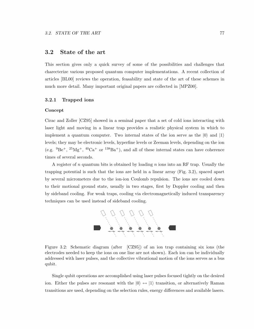
3.2. STATE OF THE ART 77
3.2 State of the art
This section gives only a quick survey of some of the possibilities and challenges that
charecterize various proposed quantum computer implementations. A recent collection of
articles [BL00] reviews the operation, feasability and state of the art of these schemes in
much more detail. Many important original papers are collected in [MPZ00].
3.2.1 Trapped ions
Concept
Cirac and Zoller [CZ95] showed in a seminal paper that a set of cold ions interacting with
laser light and moving in a linear trap provides a realistic physical system in which to
implement a quantum computer. Two internal states of the ion serve as the |0〉 and |1〉levels; they may be electronic levels, hyperfine levels or Zeeman levels, depending on the ion
(e.g. 9Be+, 25Mg+, 40Ca+ or 138Ba+), and all of these internal states can have coherence
times of several seconds.
A register of n quantum bits is obtained by loading n ions into an RF trap. Usually the
trapping potential is such that the ions are held in a linear array (Fig. 3.2), spaced apart
by several micrometers due to the ion-ion Coulomb repulsion. The ions are cooled down
to their motional ground state, usually in two stages, first by Doppler cooling and then
by sideband cooling. For weak traps, cooling via electromagnetically induced transparency
techniques can be used instead of sideband cooling.
Figure 3.2: Schematic diagram (after [CZ95]) of an ion trap containing six ions (theelectrodes needed to keep the ions on one line are not shown). Each ion can be individuallyaddressed with laser pulses, and the collective vibrational motion of the ions serves as a busqubit.
Single qubit operations are accomplished using laser pulses focused tightly on the desired
ion. Either the pulses are resonant with the |0〉 ↔ |1〉 transition, or alternatively Raman
transitions are used, depending on the selection rules, energy differences and available lasers.
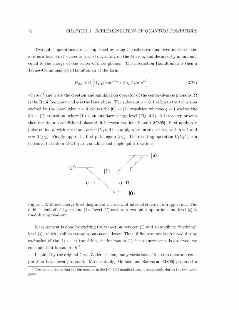
78 CHAPTER 3. IMPLEMENTATION OF QUANTUM COMPUTERS
Two qubit operations are accomplished by using the collective quantized motion of the
ions as a bus. First a laser is turned on, acting on the kth ion, and detuned by an amount
equal to the energy of one center-of-mass phonon. The interaction Hamiltonian is then a
Jaynes-Cummings type Hamiltonian of the form
Hk,q ∝ Ω[|1q〉k〈0|ae
−iφ + |0〉k〈1q|a†eiφ
], (3.29)
where a† and a are the creation and annihilation operator of the center-of-mass phonons, Ω
is the Rabi frequency and φ is the laser phase. The subscript q = 0, 1 refers to the transition
excited by the laser light; q = 0 excites the |0〉 ↔ |1〉 transition whereas q = 1 excites the
|0〉 ↔ |1′〉 transition, where |1′〉 is an auxiliary energy level (Fig. 3.3). A three-step process
then results in a conditional phase shift between two ions k and l [CZ95]. First apply a π
pulse on ion k, with q = 0 and φ = 0 (U1). Then apply a 2π pulse on ion l, with q = 1 and
φ = 0 (U2). Finally apply the first pulse again (U1). The resulting operation U1U2U1 can
be converted into a cnot gate via additional single qubit rotations.
|1’
|s
|0
|1
=1 =0q q
Figure 3.3: Model energy level diagram of the relevant internal states in a trapped ion. Thequbit is embodied by |0〉 and |1〉. Level |1′〉 assists in two qubit operations and level |s〉 isused during read-out.
Measurement is done by exciting the transition between |1〉 and an auxiliary “shelving”
level |s〉, which exhibits strong spontaneous decay. Thus, if fluorescence is observed during
excitation of the |1〉 ↔ |s〉 transition, the ion was in |1〉; if no fluorescence is observed, we
conclude that it was in |0〉.7
Inspired by the original Cirac-Zoller scheme, many variations of ion trap quantum com-
putation have been proposed. Most notably, Mølmer and Sørenson [MS99] proposed a7The assumption is that the ion remains in the |0〉, |1〉manifold except temporarily during the two-qubit
gates.
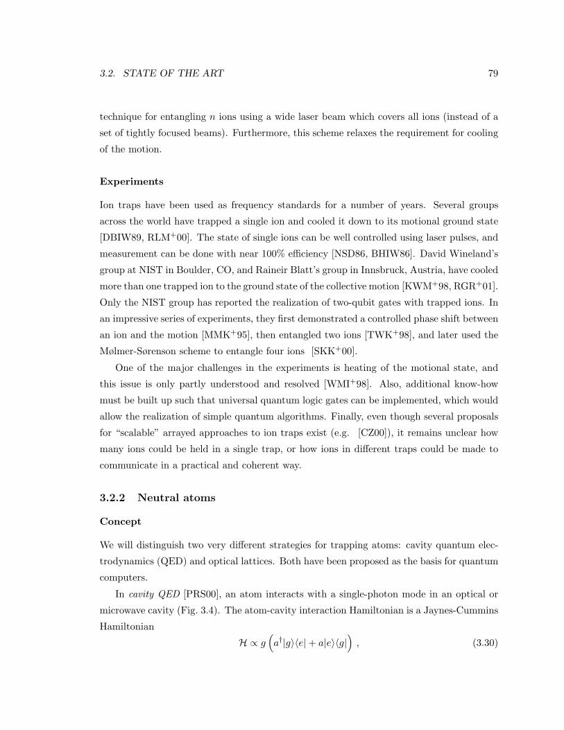
3.2. STATE OF THE ART 79
technique for entangling n ions using a wide laser beam which covers all ions (instead of a
set of tightly focused beams). Furthermore, this scheme relaxes the requirement for cooling
of the motion.
Experiments
Ion traps have been used as frequency standards for a number of years. Several groups
across the world have trapped a single ion and cooled it down to its motional ground state
[DBIW89, RLM+00]. The state of single ions can be well controlled using laser pulses, and
measurement can be done with near 100% efficiency [NSD86, BHIW86]. David Wineland’s
group at NIST in Boulder, CO, and Raineir Blatt’s group in Innsbruck, Austria, have cooled
more than one trapped ion to the ground state of the collective motion [KWM+98, RGR+01].
Only the NIST group has reported the realization of two-qubit gates with trapped ions. In
an impressive series of experiments, they first demonstrated a controlled phase shift between
an ion and the motion [MMK+95], then entangled two ions [TWK+98], and later used the
Mølmer-Sørenson scheme to entangle four ions [SKK+00].
One of the major challenges in the experiments is heating of the motional state, and
this issue is only partly understood and resolved [WMI+98]. Also, additional know-how
must be built up such that universal quantum logic gates can be implemented, which would
allow the realization of simple quantum algorithms. Finally, even though several proposals
for “scalable” arrayed approaches to ion traps exist (e.g. [CZ00]), it remains unclear how
many ions could be held in a single trap, or how ions in different traps could be made to
communicate in a practical and coherent way.
3.2.2 Neutral atoms
Concept
We will distinguish two very different strategies for trapping atoms: cavity quantum elec-
trodynamics (QED) and optical lattices. Both have been proposed as the basis for quantum
computers.
In cavity QED [PRS00], an atom interacts with a single-photon mode in an optical or
microwave cavity (Fig. 3.4). The atom-cavity interaction Hamiltonian is a Jaynes-Cummins
Hamiltonian
H ∝ g(a†|g〉〈e|+ a|e〉〈g|
), (3.30)

80 CHAPTER 3. IMPLEMENTATION OF QUANTUM COMPUTERS
where a† and a are the raising and lowering operator of the cavity, |g〉 and |e〉 are the
ground and excited states of the atom and g is the vacuum Rabi frequency. The coherent
interaction of the atom and the cavity competes with spontaneous decay of the atom at
a rate γ and with cavity decay at a rate κ. In order to obtain “strong” coupling between
the atom and the cavity, we need g (γ, κ), and the dwell time of the atom in the cavity
must be long compared to the inverse of these rates. A high value of γ requires a small
cavity (only about 10 µm long) so the electric field of the single photon is very intense; κ
is determined by the reflectivity of the mirrors and γ depends on the atom and also on the
cavity.
Such cavities, in particular microwave cavities, could in principle be used for quantum
computation, with two internal levels of the atom (|g〉 and |e〉) as a qubit. A register of
several qubits could be realized by trapping several atoms in a cavity. Tighly focused laser
beams coming in from the sides of the cavity could address individual atoms for one-qubit
gates, and the cavity mode could serve as a bus qubit for two-qubit gates, as it interacts
with all the atoms. However, such schemes appear very difficult to realize.
mirror
cavity
g κ
γ
atom
Figure 3.4: A single two-level atom is trapped by the cavity mode of a single photon. Thecavity consists of two curved mirrors. (after Mabuchi in [MPZ00])
A more suitable application of cavity-QED, especially for optical cavities, may lie in the
area of quantum communication. A trapped atom could mediate an interaction between
“flying” (photon) qubits. Furthermore, appropriate excitation of an atom trapped in a
cavity could emit single photons in a controlled way, and thus serve as a source for quantum
cryptography. In microwave cavities, an atom travelling through the cavity could transfer
its quantum information to the cavity, which in turn could transfer the information to a
second atom travelling through the cavity at a later time. All these schemes illustrate that
atom-cavity interactions provide a rich system for the exchange of quantum information
between “flying” qubits and “standing” qubits.

3.2. STATE OF THE ART 81
Atoms trapped in far off-resonance optical lattices have also been proposed as qubits
[BCJD99, DB00]. An optical lattice is created by three sets of optical standing waves at
right angles, created by laser beams. A large number of neutral atoms can be loaded into
the optical lattice for example from a magneto-optical atom trap or from a Bose-Einstein
condensate; the atoms are trapped by the lattice at regular spacings in the “wells” of the
standing waves. On-resonance laser beams can produce single-qubit rotations. By varying
the polarization of the trapping lasers, two sets of atoms in adjacent wells can be made to
pairwise occupy the same well so electric dipole-dipole interactions between the two atoms
in each pair are induced. Two-qubit gates are thus be performed on many pairs of atoms in
parallel, which can be advantageous in some cases but also constitutes a limitation. Good
ways to measure the internal state of atoms trapped in an optical lattice are currently being
investigated.
Experiments
Strong atom-cavity coupling has been achieved in both optical cavities, most notably with
Cs atoms in Kimble’s group at Caltech, [MTCK96] and with Rydberg atoms in microwave
cavities, in Haroche’s lab at the ENS in Paris [BSKM+96]. An atom trapped in an optical
cavity has been used to cause a conditional phase shift between two photons flying through
the cavity and interacting with the atom [THL+95]. This experiment represented the first
explicit realization of a two-qubit gate. An optical cavity has been used as a single-photon
source [LK97] and quantum memory operation of a single photon mode has been accom-
plished in a microwave cavity [MHN+97]. Also via a microwave cavity, three Rydberg atoms
have been entangled with each other [RNO+00].
Compared to trapped ions, coherent control and readout are more complicated in
trapped atoms, since the trapping potentials are much weaker for neutral atoms than for
charged ions. For this and other reasons, it appears that the potential of cavity QED for
quantum computing is limited, but optical cavities may find good use in quantum commu-
nication. Both optical and microwave cavities also provide a beautiful testbed for the study
of decoherence and quantum (non-demolition) measurements, as in [NRO+99].
The state of the art in optical lattices is still extremely limited. On the order of 106
neutral Cs atoms have been trapped in a two-dimensional lattice [HHK+98], but it is not
currently possible to reliably create a completely full lattice, much less to selectively control
or read out the state of atoms trapped in an optical lattice.
82 CHAPTER 3. IMPLEMENTATION OF QUANTUM COMPUTERS
3.2.3 Quantum dots
Loss and DiVincenzo [LD98] worked out a proposal for quantum computing based on “ar-
tificial atoms”, created via semiconductor structures. In such quantum dots, the qubit is
given by the spin of the excess electron on a single-electron quantum dot, placed in a static
magnetic field. The confinement of the electron in the dot must be strong enough such
that excited excitonic and electronic states have much higher energies than the spin Zee-
man energy, and thus have negligable occupancy. The lay out of a possible device is shown
schematically in Fig. 3.5.
Figure 3.5: Conceptual schematic (after [DL99]) of one variant of a quantum dot quantumcomputer. Lateral side gates on top of a two-dimensional electron gas (created for examplevia a AlGaAs/GaAs/AlGaAs quantum well) confine the motion of an electron to a verysmall area (the quantum dot). The tunneling barrier between neighbouring quantum dotscan be controlled via the voltages on the gates.
One-qubit rotations could be realized in several ways. Via advanced scanning probe
techniques, it may be possible to locally and selectively manipulate the electron spin in
just one quantum dot. Alternatively, the Larmor frequency of the electron could be shifted
selectively by changing the bias on the side gates of a specific dot, or by opening a tunneling
barrier to an auxiliary dot which is ferro-magnetic. A narrowband microwave transverse
magnetic field can then selectively rotate the spin of the electron on a specific dot.
Two-qubit gates rely on the exchange interaction between the electrons in adjacent dots,
which arises from tunneling through the barrier between the dots:
H = J ~I1 · ~I2 . (3.31)
By gating the tunneling barrier via the side gates, this interaction can be turned on and off
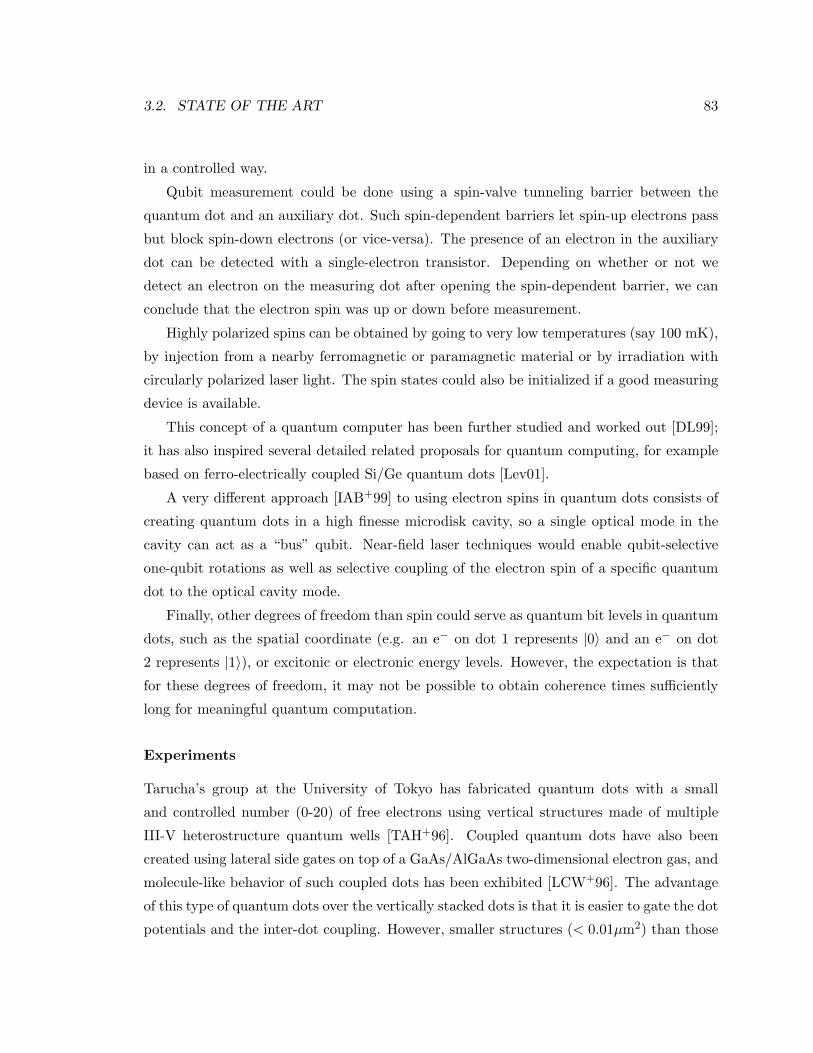
3.2. STATE OF THE ART 83
in a controlled way.
Qubit measurement could be done using a spin-valve tunneling barrier between the
quantum dot and an auxiliary dot. Such spin-dependent barriers let spin-up electrons pass
but block spin-down electrons (or vice-versa). The presence of an electron in the auxiliary
dot can be detected with a single-electron transistor. Depending on whether or not we
detect an electron on the measuring dot after opening the spin-dependent barrier, we can
conclude that the electron spin was up or down before measurement.
Highly polarized spins can be obtained by going to very low temperatures (say 100 mK),
by injection from a nearby ferromagnetic or paramagnetic material or by irradiation with
circularly polarized laser light. The spin states could also be initialized if a good measuring
device is available.
This concept of a quantum computer has been further studied and worked out [DL99];
it has also inspired several detailed related proposals for quantum computing, for example
based on ferro-electrically coupled Si/Ge quantum dots [Lev01].
A very different approach [IAB+99] to using electron spins in quantum dots consists of
creating quantum dots in a high finesse microdisk cavity, so a single optical mode in the
cavity can act as a “bus” qubit. Near-field laser techniques would enable qubit-selective
one-qubit rotations as well as selective coupling of the electron spin of a specific quantum
dot to the optical cavity mode.
Finally, other degrees of freedom than spin could serve as quantum bit levels in quantum
dots, such as the spatial coordinate (e.g. an e− on dot 1 represents |0〉 and an e− on dot
2 represents |1〉), or excitonic or electronic energy levels. However, the expectation is that
for these degrees of freedom, it may not be possible to obtain coherence times sufficiently
long for meaningful quantum computation.
Experiments
Tarucha’s group at the University of Tokyo has fabricated quantum dots with a small
and controlled number (0-20) of free electrons using vertical structures made of multiple
III-V heterostructure quantum wells [TAH+96]. Coupled quantum dots have also been
created using lateral side gates on top of a GaAs/AlGaAs two-dimensional electron gas, and
molecule-like behavior of such coupled dots has been exhibited [LCW+96]. The advantage
of this type of quantum dots over the vertically stacked dots is that it is easier to gate the dot
potentials and the inter-dot coupling. However, smaller structures (< 0.01µm2) than those
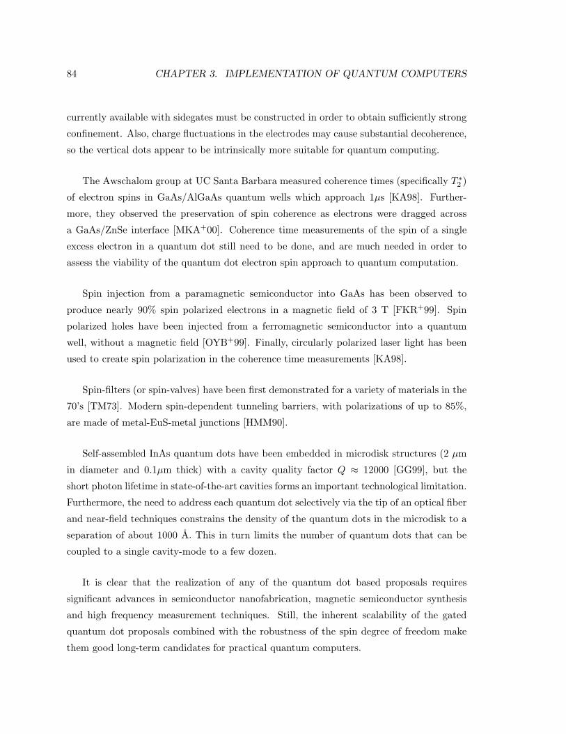
84 CHAPTER 3. IMPLEMENTATION OF QUANTUM COMPUTERS
currently available with sidegates must be constructed in order to obtain sufficiently strong
confinement. Also, charge fluctuations in the electrodes may cause substantial decoherence,
so the vertical dots appear to be intrinsically more suitable for quantum computing.
The Awschalom group at UC Santa Barbara measured coherence times (specifically T ∗2 )
of electron spins in GaAs/AlGaAs quantum wells which approach 1µs [KA98]. Further-
more, they observed the preservation of spin coherence as electrons were dragged across
a GaAs/ZnSe interface [MKA+00]. Coherence time measurements of the spin of a single
excess electron in a quantum dot still need to be done, and are much needed in order to
assess the viability of the quantum dot electron spin approach to quantum computation.
Spin injection from a paramagnetic semiconductor into GaAs has been observed to
produce nearly 90% spin polarized electrons in a magnetic field of 3 T [FKR+99]. Spin
polarized holes have been injected from a ferromagnetic semiconductor into a quantum
well, without a magnetic field [OYB+99]. Finally, circularly polarized laser light has been
used to create spin polarization in the coherence time measurements [KA98].
Spin-filters (or spin-valves) have been first demonstrated for a variety of materials in the
70’s [TM73]. Modern spin-dependent tunneling barriers, with polarizations of up to 85%,
are made of metal-EuS-metal junctions [HMM90].
Self-assembled InAs quantum dots have been embedded in microdisk structures (2 µm
in diameter and 0.1µm thick) with a cavity quality factor Q ≈ 12000 [GG99], but the
short photon lifetime in state-of-the-art cavities forms an important technological limitation.
Furthermore, the need to address each quantum dot selectively via the tip of an optical fiber
and near-field techniques constrains the density of the quantum dots in the microdisk to a
separation of about 1000 A. This in turn limits the number of quantum dots that can be
coupled to a single cavity-mode to a few dozen.
It is clear that the realization of any of the quantum dot based proposals requires
significant advances in semiconductor nanofabrication, magnetic semiconductor synthesis
and high frequency measurement techniques. Still, the inherent scalability of the gated
quantum dot proposals combined with the robustness of the spin degree of freedom make
them good long-term candidates for practical quantum computers.

3.2. STATE OF THE ART 85
3.2.4 Superconducting qubits
Concept
The superconducting qubit proposals differ from all the other proposals discussed here
in that the qubit is represented by two quantized states which are collective states of a
“macroscopic” number of particles: flux states resulting from the motion of millions to
billions of Cooper pairs through a SQUID or charge states produced by millions of Cooper
pairs in a “box”.
Josephson junctions play a central role in both approaches [Ave00]: if the charging
energy EC = e2/2CJ (with CJ the capacitance of the Josephson junction) is much larger
than the Josephson coupling energy EJ , the device is charge-dominated. In contrast, if
EC EJ , the device is dominated by the phase across the junction, which is the conjugate
variable of the charge (or equivalently the number) of the excess electrons on one side of
the junction.
Flux qubits [MOL+99] are given by two energy levels of the quantized flux through a
superconducting ring with one or more Josephson junctions in the phase regime (Fig. 3.6).
In a micrometer sized loop, each flux state arises from the collective motion of up to 109
Cooper pairs producing a µA current through the loop.
CE ,J J
qubit 1 qubit 2
coupling loop
Josephson Junction
Figure 3.6: Schematic of two superconducting flux qubits, each embodied by a small su-perconducting loop interrupted by Josephson junctions (small barriers made of a resistivematerial). The devices shown contain three Josephson junctions, as in [vtW+00].
Several schemes have been proposed for logic gates. One-qubit rotations involve the
application of local magnetic fields which change the environment of a specific qubit. In
addition, by changing the parameters of the Josephson junctions, one-qubit operations can
be performed in different basis. The interaction mechanism for two-qubit gates is inductive
86 CHAPTER 3. IMPLEMENTATION OF QUANTUM COMPUTERS
coupling between neighbouring loops. This coupling can be enhanced via a separate super-
conducting coupling loop with encloses the two qubits (Fig. 3.6), or alternatively the two
loops can be part of the same superconducting circuit.
Measurement of the flux state of a qubit can be done using a DC measuring SQUID (not
shown in the figure), either enclosing the qubit or placed next to the qubit. Unfortunately,
it is not possible with current technology to switch the measuring SQUID off by opening
the measuring loop, so the coupling between the measuring SQUID and the qubit must be
very weak in order to prevent excessive decoherence. Of course, the flip side of very weak
coupling is that extensive signal averaging is required in the measurement.
Charge qubits [MSS99] rely on the quantized number of excess electrons on a small
superconducting island when it is coupled to the ground by a number-state dominated
Josephson junction (Fig. 3.7). As for flux qubits, one-qubit operations can be realized via
local magnetic fields. Two qubit operations can be done by embedding multiple charge
qubits in parallel in a larger circuit, so the different qubits are coupled. The number of
excess Cooper pairs on the box can be measured via a probe Josephson junction through
which Cooper pairs can tunnel out of the box, depending on the charge state of the box
and on the probe voltage Vp (Fig. 3.7).
JC
JE ,
V
C
g
box
Vp
Figure 3.7: Schematic of a superconducting charge qubit, realized by a small supercon-ducting island or “box”, coupled to the ground via a Josephson junction. The electrostaticpotential of the island is controlled by the gate voltage Vg. The dashed part of the circuitserves for readout; it is not part of the actual qubit. In practice, improved variations ofthis design are used, which use more Josephson junctions in order to be able to have morecontrol over the qubit parameters.
Both the charge qubit and the flux qubit devices must be operated at low temperature
(say 20 mK, which is well below the critical temperature of Al or other superconducting
materials of choice), such that the ground state is occupied with probability near 1.

3.2. STATE OF THE ART 87
Experiments
Nakamura and coworkers at NEC in Tsukuba have observed evidence for coherent super-
positions of two charge states in a single-Cooper-pair box [NCT97]. The energy levels were
shifted via a gate-induced charge e (Fig. 3.7) such that the energies of the two lowest levels
(and excess charge of 0 and 2e) would become equal (while the next lowest level is at a
much higher energy); however, the Josephson energy splits these two levels and the result-
ing eigenstates are coherent superpositions of two collective states of a macroscopic number
of Cooper pairs, which differ in charge by 2e. Energy level splitting was experimentally
observed, which suggests that the box was in a coherent superposition of two charge states
[NCT97]. Later, the same group demonstrated coherent control of the quantum states in the
single-Cooper-pair box, via pulsed experiments and time domain measurements of multiple
Rabi oscillations [NPT99].
The groups of Mooij at Delft and Lukens at SUNY Stony Brook both observed simi-
lar evidence for macroscopic superpositions of flux states in small SQUID loops [FPC+00,
vtW+00]. Here the classical energy of two flux states was made equal via an externally
applied static magnetic field. When quantum tunneling between these two states of equal
energy is possible, the loop’s eigenstates become the symmetric and antisymmetric super-
position of the original flux states. The creation of such superposition states was deduced
from the observation of energy level splitting. No time domain measurements demonstrating
coherent control have been performed to date in these systems.
Even though the state of the art is currently more advanced in charge qubits than in
flux qubits, the expectation is that flux qubits have longer coherence times than charge
qubits, so flux states may be better qubits than charge states. Measurements of coherence
times in either system would represent significant progress in evaluating superconducting
qubit proposals.
3.2.5 Solid-state NMR
Concept
In a very different solid-state approach, Yamaguchi and Yamamoto [YY99] propose the use
of nuclear spins in a crystal lattice as quantum bits (Fig. 3.8). In this proposal, which
was further developed by the same group [LGD+00], a quantum computer consists of a
one-dimensional array of spin-1/2 nuclei spaced by a few A along the z axis; the presence

88 CHAPTER 3. IMPLEMENTATION OF QUANTUM COMPUTERS
of a magnetic field with a strong gradient along z (on the order of 1 T/µm) separates the
Larmor frequency of the qubits so they can be individually distinguished and addressed.
1
2
3C
B
Aa
b
c
x
z y
Figure 3.8: Model of a crystal lattice quantum computer. The crystal shown here has asimple cubic lattice; in practice other lattices have been proposed, but the idea is the same.The nuclei 1, 2, 3, . . . form one quantum computer, the nuclei a, b, c, . . . form an independentcomputer, and so forth. Nuclei 1, a and A represent the analogous qubit in the respectivecomputers.
In the transverse direction, the magnetic field must be homogeneous so the crystal
contains many identical copies of this one-dimensional chain of nuclei. All the copies operate
as independent quantum computers provided the interactions between them are switched
off. An important advantage of such a scheme is that the measurement of a qubit can
take place over a large ensemble of nuclear spins instead of just a single nuclear spin as is
required in the Kane proposal (section 3.2.6).
Two qubit gates rely on the magnetic dipole-dipole coupling between spins in the same
computer. With both the magnetic field and the strong field gradient along the direction of
the chain of spins z, the coupling Hamiltonian between two spins i and j within the same
chain is of the form
Hi,j ∝IizI
jz
(|j − i|a)3, (3.32)
where a is the distance between neighbouring nuclei. This Hamiltonian is easy to work with
and can be selectively suppressed simply by applying a suitable periodic train of narrowband
180 pulses [LCYY00].
3.2. STATE OF THE ART 89
The coupling between spins in different copies has a different form. For two spins with
the same Larmor frequency but located in different chains m and n (i.e. analogous qubits
in different computers), the coupling Hamiltonian is of the form
Hmn ∝1− 3 cos2 θmn
(aλmn)3
(3Imz I
nz − ~Im · ~In
), (3.33)
where λmn is the distance between the two nuclei in units of a and θmn is the angle between
the vector which connects them and the direction of the applied field z. This coupling can
be largely switched off as well, using well-known solid-state NMR broadband decoupling
pulse sequences, such as the WAHUHA sequence [Meh83].
The WAHUHA pulse sequence also affects the qubit-qubit coupling of Eq. 3.32 but this
coupling can still be sufficiently controlled for two-qubit gates using additional narrowband
pulses. However, the coupling between qubits with different resonance frequencies (i 6= j)
and in different chains (m 6= n) is partially reintroduced during such two-qubit gates, and
causes decoherence. Fortunately, this effect can be kept quite small by choosing a very
one-dimensional crystal, for example fluorapatite, Ca5F(PO)4)3, where the 19F nuclei serve
as qubits [LGD+00].
Unlike for liquid NMR, state initialization can in principle be done by cooling down the
sample to the milli-Kelvin regime. In practice, such low temperature may be difficult to
maintain given the many RF pulses involved in broadband decoupling. Optical pumping or
polarization transfer from electron spins may then be needed.
Readout is much helped by the ensemble nature of the experiment; even for a relatively
small crystal, there are on the order of 107 members in the ensemble. Given the presence of a
strong magnetic field gradient, magnetic resonance force microscopy using microcantilevers
[RYS92] has been proposed as a natural way to measure the spin states.
The main source of decoherence in this system is residual dipolar couplings. Further-
more, magnetic impurities and cantilever drift ( as the sample would be mounted on the
cantilever) also contribute to decoherence.
An indepedent but less detailed proposal for solid-state NMR quantum computing was
presented by Cory et al. [CLK+00]. The main difference with the crystal lattice proposal is
that in the Cory scheme the quantum computer would be an ensemble of specially designed
molecules, held and aligned in a solid state lattice.

90 CHAPTER 3. IMPLEMENTATION OF QUANTUM COMPUTERS
Experiments
Solid-state NMR has a tradition of over 50 years, and coherence times and decoherence
mechanisms have been studied since the early days [Blo49]. The T1 of nuclear spins in
reasonably pure crystals is limited by thermal fluctuations of paramagnetic impurities but
can easily be several hours. While T2 is typically only on the order of milliseconds due
to dipolar broadening, it can be lengthened by several orders of magnitude using well-
established broadband decoupling techniques which have proven their effectiveness.
Growth of high purity crystals of fluorapatite is relatively well understood. Furthermore,
force microscopy with sufficient sensitivity to detect 107 nuclear spins has been demon-
strated [SMY+01].
No actual quantum logic gates have been implemented yet, but the crystal lattice quan-
tum computer has the potential for scaling up to several hundred qubits, and experiments
are underway. The main challenge lies in the integration and alignment of the different com-
ponents, and the design of a micromagnet which produces a strong magnetic field which is
uniform along two axes but has a steep gradient along the third axis.
The approach based on molecules in solid solutions aims at intermediate sized quantum
computers containing several tens of qubits. Here also, experiments are underway.
3.2.6 Dopants in semiconductors
Bruce Kane, of the University of Maryland, proposed an approach which integrates solid-
state NMR on donor atoms with semiconductor electronics [Kan98]; this scheme has some
conceptual similarities with the quantum dot scheme of section 3.2.3. The quantum bits
are embodied by the spin-1/2 nucleus of 31P dopants arranged in a regular array below the
surface of a silicon substrate (Fig. 3.9), placed in a static magnetic field perpendicular to
the surface.
A A AJ J
Si substrate
barrier
31P 31P 31P+ + +
Figure 3.9: Model of a Kane-type quantum computer (cross-section), after [Kan98].
Phosphorus in silicon is an electron donor at room temperature, but at low temperatures
3.2. STATE OF THE ART 91
(100 mK), the electron is weakly bound to the phosporus ion. A voltage applied to the A
gate located about 200 A above a specific 31P ion, shifts the electron away from that nucleus
and thereby reduces the hyperfine interaction. As a result, the energy difference between
the spin-up and spin-down state of the nuclear spin changes and a radio-frequency pulse
can then selectively rotate the state of the one 31P nuclear spin for which the A gate is
biased.
Two-qubit gates between adjacent phosphorus nuclei rely on an indirect coupling mech-
anism mediated by their respective electrons. The coupling Hamiltonian of two donor-
electron spin systems is
H = A1~I 1n · ~I 1e +A2
~I 2n · ~I 2e + J~I 1e · ~I 2e (3.34)
where A1 and A2 are the hyperfine interaction energies and J is the exchange energy.
In order to obtain reasonable values of J (> 10 GHz), the donor separation must be no
more than 100-200 A. A negative voltage applied to the J gate in between two 31P nuclei
repels the electrons and dimishes their overlap. Because J is proportional to the electron
wavefunction overlap, the e−-e− interaction can thus be turned off at will via the J gates.
Measurement of the 31P nuclear spin states is done in an innovative two-step process.
First, the A gate of the nuclear spin we want to measure, say spin i, is biased, while the A
gate of a neighbouring nuclear spin, j, is not (Ai > Aj). Under these conditions, the J gate
between the two dopant atoms i and j is ramped up such that J > µBB/2 and therefore
the singlet state (|↑↓〉 − |↓↑〉)/√
2 becomes the lowest energy state of the two electron spins
(during the computation, J < µBB/2 so the ground state of the two electron spins is |↓↓〉).The electron spins will then adiabatically evolve into the singlet state if spin i is in |0〉,whereas they remain in the metastable state |↓↓〉 if spin i is in |1〉; the state of spin j is
inconsequential. In the second step, the electron spin state is measured electronically. Both
electrons can be bound to the same donor by biasing the A gates appropriately provided
the electron spins are in (|↑↓〉 − |↓↑〉)/√
2; if the electron spins are in |↓↓〉, the electrons
cannot be bound to the same donor. Thus, by alternating the voltage applied to the two
respective A gates, charge motion can be induced between the two donors if and only the
electrons are in the singlet state, which in turns depends on the state of nuclear spin i. The
charge motion can be detected via a single-electron transistor.
The electron spins are initialized to the ground state by working at 2 T and 100 mK.

92 CHAPTER 3. IMPLEMENTATION OF QUANTUM COMPUTERS
The nuclear spin can be initialized via the measurement process: measure the nuclear spin
and flip it if necessary.
Voltage fluctuations in the control gates, especially the A gates, are expected to con-
tribute to decoherence, as the Larmor precession frequency of the nuclear spins is affected
by the voltage on the A electrodes. More signficantly, the presence of a single-electron
transistor also induces relaxation, at an estimated rate of 1 kHz.
The Kane proposal inspired a related proposal by Eli Yablonovitch and coworkers
[VYW+99]. There are two main differerences with the Kane scheme: (1) the donor electron
spin represents the qubit, instead of the dopant nuclear spin; (2) there are no J gates; both
one-qubit and two-qubit gates could be realized using A gates, which is made possible by
using silicon-germenium heterostructures, bandgap engineering and g factor engineering.
Experiments
The fabrication technology required for a Kane-type computer is still beyond the state of
the art: it is not currently possible to deposit individual phosphorus atoms over large areas
and with atomic precision below a silicon surface, nor can we pattern many electrodes of
only 50 A wide and spaced by 200 A. Alignment of the gates with respect to the buried
dopant atoms represents an additional challenge. Finally, further advances in materials
technology would be needed to obtain highly pure 28Si (the natural abundance of 29Si is
about 5%), and nearly defect-free oxide barriers.
Nevertheless, Kane’s proposal is very appealing for its scalability and elegance, and
provides a strong motivation for developing the necessary technology. In a first step towards
the fabrication of a Kane-type quantum computer, atomic hydrogen has been adsorbed on
a silicon surface, hydrogen desorbed with an STM tip over an area of 1 nm across, and
single phosphine molecules have been adsorbed onto the silicon substrate through the 1 nm
holes in the hydrogen layers [OSS+01].
Measurements of T1 have been done long ago [FG59]. The electron spin T1 at low 31P
concentrations in pure 28Si and at 1.5 K has been measured to be thousands of seconds; the
phosphorus spin T1 was over 10 hours. At 100 mK, even longer T1’s are expected. Finally,
Rabi oscillations have been observed between two low-lying hydrogen-atom like states of an
electron weakly bound to a donor impurity in GaAs [CWK+01].
The Yablonovitch variant puts less demands on lithography, as only one gate must be
fabricated per qubit, and in addition the spacing between the qubits can be much larger than

3.3. SUMMARY 93
in the original proposal (up to 200 nm). On the other hand, there are additional demands
on epitaxial growth techniques due to the need for bandgap and g factor engineering.
3.2.7 Other proposals
Several other proposals exist for the implementation of quantum computers, in addition to
those we have discussed in the preceding sections. We will just mention two of them.
Platzman and Dykman suggested the use of a quasi-two dimensional set of electrons
floating in vacuum above liquid helium [PD99]. Individual electrons are laterally confined
by micrometer sized electrodes below the helium, and strongly interact with neighbouring
electrons. The qubit states are given by the lowest hydrogenic levels, at 10 mK. Locally
applied electric fields would produce one-qubit gates and read-out would be done by selec-
tively releasing excited electrons from the surface, and absorbing them in an electrometer
placed above the surface.
There also exist proposals for all-optical quantum computers [Mil89]. The main obstacle
to such devices, the high losses associated with sufficiently non-linear optical elements, was
recently circumvented by a proposed scheme for efficient quantum computation with just
linear optics [KLM01] (see page 64).
3.3 Summary
Today’s technology enables physicists to separately meet any one of the five requirements
for building a quantum computer exceedingly well. For example, it is possible already to
1. integrate tens of thousands of quantum dots on a single chip using semiconductor
technology,
2. realize extremely precise two-qubit gates using the natural coupling between neigh-
bouring spins,
3. reliably initialize an atom to its internal ground state by atomic cooling techniques,
4. perform near-ideal measurements of the internal state of trapped ions using fluores-
cence techniques,
5. obtain lifetimes of several days for nuclear spins in solids.
94 CHAPTER 3. IMPLEMENTATION OF QUANTUM COMPUTERS
Furthermore, we have seen that many of the traditional requirements for the physical re-
quirements of quantum computers can be relaxed or circumvented.
Nevertheless, satisfying all five criteria within one device still remains an extraordi-
nary challenge which hasn’t been met in any of these systems. In fact, it has not been
possible so far to realize even the simplest quantum algorithms with any of the proposed
implementations we have discussed.
The crucial difficulty can be summarized as follows: on the one hand, long coherence
times require that the qubits be highly isolated from the environment; on the other hand,
we must have external access to the qubits in order to initialize, control and read out their
state. The system which best reconciles these opposing requirements will eventually come
out as the “winning” quantum computer realization.
In the next chapter, we describe in detail an experimental system which we haven’t yet
discussed, but which, as we shall see, truly stands out in its accessibility: nuclear spins in
molecules disolved in liquid solution, and manipulated by magnetic resonance techniques.
Chapter 4
Liquid-state NMR quantum
computing
In this chapter, we will examine whether nuclear spins in molecules in liquid solution satisfy
the five requirements for the implementation of quantum computers. One section will be
devoted to each requirement, except that single-qubit gates and two-qubit gates are treated
in separate sections. Based on this discussion, we will close with guidelines for molecule
design and NMR pulse sequence design.
4.1 Qubits
The qubits in NMR quantum computing are given by the spins of suitable atomic nuclei,
placed in a static magnetic field ~B0.
We shall here be exclusively interested in spin-1/2 nuclei, such as 1H, 13C, 15N,19F and 31P, as they have two discrete eigenstates.
Spin-0 nuclei, for example 12C and 16O, are not magnetic and therefore not detectable with
NMR. Nuclei with spin quantum number greater than 1/2, such as 2H, 14N, 35Cl, 37Cl,79Br and 81Br, don’t make for good qubits either; mapping the larger number of states (e.g.
the spin quantum number of a spin-3/2 particle can be −3/2,−1/2, 1/2 or 3/2) onto qubit
states, and performing quantum logic gates on them, introduces additional complications.
More significantly, nuclear spins with spin > 1/2 tend to have very short coherence times.
95

96 CHAPTER 4. LIQUID-STATE NMR QUANTUM COMPUTING
4.1.1 Single-spin Hamiltonian
The Hamiltonian of a spin 1/2 particle in a magnetic field of strength B0 along the z axis
is [Fre97, EBW87] 1
H0 = −~γB0 Iz = −~ω0 Iz =[−~ω0/2 0
0 ~ω0/2
], (4.1)
where γ is the gyromagnetic ratio of the nucleus and ω0/2π is the Larmor frequency of the
spin (we will sometimes leave the factor of 2π implicit and call ω0 the Larmor frequency).
Iz is the angular momentum operator in the z direction, which relates to the well-known
Pauli matrix as 2Iz = σz; similarly, we will later use 2Ix = σx and 2Iy = σy.
The interpretation of Eq. 4.1 is that the energy of the |0〉 or |↑〉 state (given by 〈0|H|0〉,the upper left element of H) is lower than the energy of |1〉 or |↓〉 (〈1|H|1〉) by an amount
~ω0, as illustrated in the energy diagram of Fig. 4.1. The energy splitting is known as the
Zeeman splitting.
|1
|0
ωh
Figure 4.1: Energy diagram for a single spin-1/2.
The time evolution e−iHt/~ of the spin state under the Hamiltonian of Eq. 4.1 corresponds
to a precession motion in the Bloch sphere (Fig. 2.1) about the axis of the static magnetic
field, similar to the precession of a spinning top about the axis of gravitation, as shown in
Fig. 4.2. The B0 field is typically on the order of 10 Tesla, resulting in precession frequencies
ω0 of a few hundred MHz, which is in the radio-frequency range .
Distinguishing the nuclear spins in a molecule
A molecule with n distinguishable spin-1/2 nuclei constitutes an n-qubit quantum computer.
Spins of different nuclear species (heteronuclear spins) can be easily distinguished spectrally,
1Some authors use a different convention, leaving out the minus sign in Eq. 4.1.
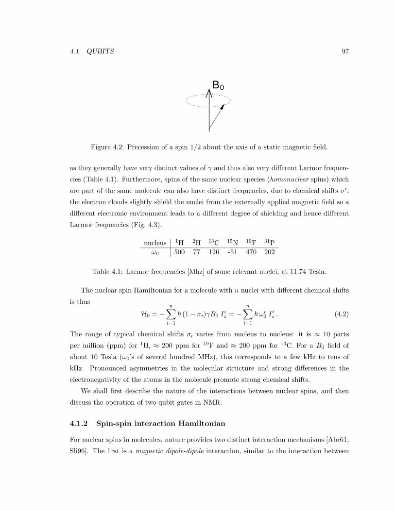
4.1. QUBITS 97
0B
Figure 4.2: Precession of a spin 1/2 about the axis of a static magnetic field.
as they generally have very distinct values of γ and thus also very different Larmor frequen-
cies (Table 4.1). Furthermore, spins of the same nuclear species (homonuclear spins) which
are part of the same molecule can also have distinct frequencies, due to chemical shifts σi:
the electron clouds slightly shield the nuclei from the externally applied magnetic field so a
different electronic environment leads to a different degree of shielding and hence different
Larmor frequencies (Fig. 4.3).
nucleus 1H 2H 13C 15N 19F 31Pω0 500 77 126 -51 470 202
Table 4.1: Larmor frequencies [Mhz] of some relevant nuclei, at 11.74 Tesla.
The nuclear spin Hamiltonian for a molecule with n nuclei with different chemical shifts
is thus
H0 = −n∑i=1
~ (1− σi)γB0 Iiz = −
n∑i=1
~ωi0 Iiz . (4.2)
The range of typical chemical shifts σi varies from nucleus to nucleus: it is ≈ 10 parts
per million (ppm) for 1H, ≈ 200 ppm for 19F and ≈ 200 ppm for 13C. For a B0 field of
about 10 Tesla (ω0’s of several hundred MHz), this corresponds to a few kHz to tens of
kHz. Pronounced asymmetries in the molecular structure and strong differences in the
electronegativity of the atoms in the molecule promote strong chemical shifts.
We shall first describe the nature of the interactions between nuclear spins, and then
discuss the operation of two-qubit gates in NMR.
4.1.2 Spin-spin interaction Hamiltonian
For nuclear spins in molecules, nature provides two distinct interaction mechanisms [Abr61,
Sli96]. The first is a magnetic dipole-dipole interaction, similar to the interaction between
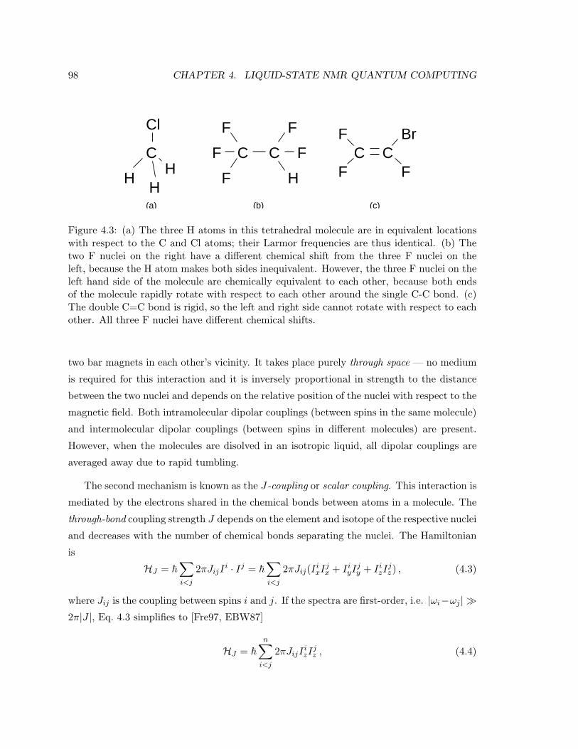
98 CHAPTER 4. LIQUID-STATE NMR QUANTUM COMPUTING
C CF
F
F
F
H
F CCF
F
F
(c)(a) (b)
BrC
Cl
HH
H
Figure 4.3: (a) The three H atoms in this tetrahedral molecule are in equivalent locationswith respect to the C and Cl atoms; their Larmor frequencies are thus identical. (b) Thetwo F nuclei on the right have a different chemical shift from the three F nuclei on theleft, because the H atom makes both sides inequivalent. However, the three F nuclei on theleft hand side of the molecule are chemically equivalent to each other, because both endsof the molecule rapidly rotate with respect to each other around the single C-C bond. (c)The double C=C bond is rigid, so the left and right side cannot rotate with respect to eachother. All three F nuclei have different chemical shifts.
two bar magnets in each other’s vicinity. It takes place purely through space — no medium
is required for this interaction and it is inversely proportional in strength to the distance
between the two nuclei and depends on the relative position of the nuclei with respect to the
magnetic field. Both intramolecular dipolar couplings (between spins in the same molecule)
and intermolecular dipolar couplings (between spins in different molecules) are present.
However, when the molecules are disolved in an isotropic liquid, all dipolar couplings are
averaged away due to rapid tumbling.
The second mechanism is known as the J-coupling or scalar coupling. This interaction is
mediated by the electrons shared in the chemical bonds between atoms in a molecule. The
through-bond coupling strength J depends on the element and isotope of the respective nuclei
and decreases with the number of chemical bonds separating the nuclei. The Hamiltonian
is
HJ = ~
∑i<j
2πJijIi · Ij = ~
∑i<j
2πJij(IixIjx + IiyI
jy + IizI
jz ) , (4.3)
where Jij is the coupling between spins i and j. If the spectra are first-order, i.e. |ωi−ωj | 2π|J |, Eq. 4.3 simplifies to [Fre97, EBW87]
HJ = ~
n∑i<j
2πJijIizIjz , (4.4)
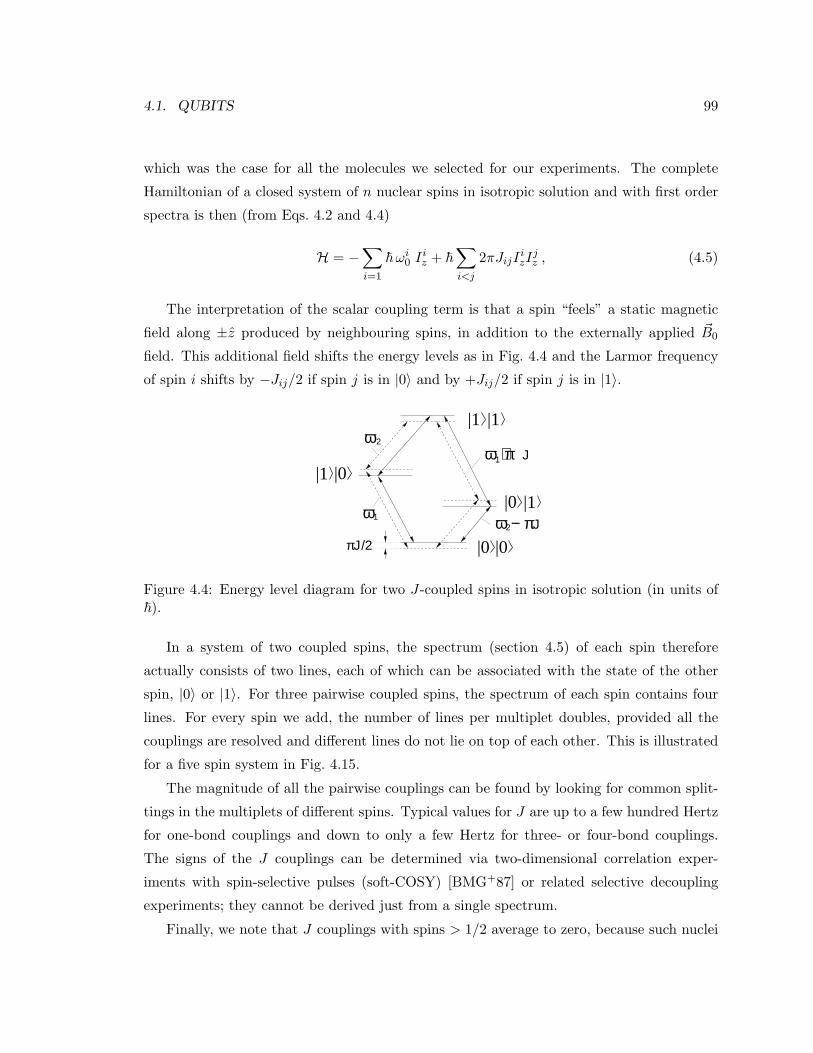
4.1. QUBITS 99
which was the case for all the molecules we selected for our experiments. The complete
Hamiltonian of a closed system of n nuclear spins in isotropic solution and with first order
spectra is then (from Eqs. 4.2 and 4.4)
H = −∑i=1
~ωi0 Iiz + ~
∑i<j
2πJijIizIjz , (4.5)
The interpretation of the scalar coupling term is that a spin “feels” a static magnetic
field along ±z produced by neighbouring spins, in addition to the externally applied ~B0
field. This additional field shifts the energy levels as in Fig. 4.4 and the Larmor frequency
of spin i shifts by −Jij/2 if spin j is in |0〉 and by +Jij/2 if spin j is in |1〉.
|1 |1
|0|1
|0 |0
|0 |1
ω + π1 J2ω
ω1
J/2π2 Jω − π
Figure 4.4: Energy level diagram for two J-coupled spins in isotropic solution (in units of~).
In a system of two coupled spins, the spectrum (section 4.5) of each spin therefore
actually consists of two lines, each of which can be associated with the state of the other
spin, |0〉 or |1〉. For three pairwise coupled spins, the spectrum of each spin contains four
lines. For every spin we add, the number of lines per multiplet doubles, provided all the
couplings are resolved and different lines do not lie on top of each other. This is illustrated
for a five spin system in Fig. 4.15.
The magnitude of all the pairwise couplings can be found by looking for common split-
tings in the multiplets of different spins. Typical values for J are up to a few hundred Hertz
for one-bond couplings and down to only a few Hertz for three- or four-bond couplings.
The signs of the J couplings can be determined via two-dimensional correlation exper-
iments with spin-selective pulses (soft-COSY) [BMG+87] or related selective decoupling
experiments; they cannot be derived just from a single spectrum.
Finally, we note that J couplings with spins > 1/2 average to zero, because such nuclei
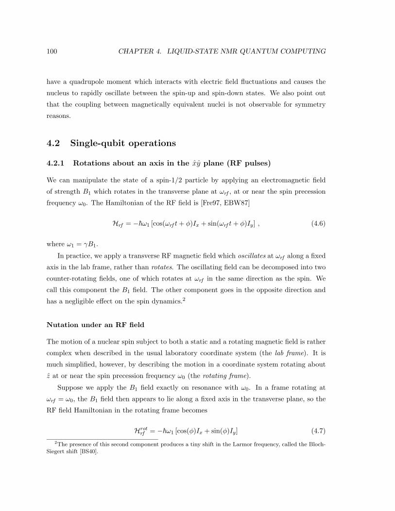
100 CHAPTER 4. LIQUID-STATE NMR QUANTUM COMPUTING
have a quadrupole moment which interacts with electric field fluctuations and causes the
nucleus to rapidly oscillate between the spin-up and spin-down states. We also point out
that the coupling between magnetically equivalent nuclei is not observable for symmetry
reasons.
4.2 Single-qubit operations
4.2.1 Rotations about an axis in the xy plane (RF pulses)
We can manipulate the state of a spin-1/2 particle by applying an electromagnetic field
of strength B1 which rotates in the transverse plane at ωrf , at or near the spin precession
frequency ω0. The Hamiltonian of the RF field is [Fre97, EBW87]
Hrf = −~ω1 [cos(ωrf t+ φ)Ix + sin(ωrf t+ φ)Iy] , (4.6)
where ω1 = γB1.
In practice, we apply a transverse RF magnetic field which oscillates at ωrf along a fixed
axis in the lab frame, rather than rotates. The oscillating field can be decomposed into two
counter-rotating fields, one of which rotates at ωrf in the same direction as the spin. We
call this component the B1 field. The other component goes in the opposite direction and
has a negligible effect on the spin dynamics.2
Nutation under an RF field
The motion of a nuclear spin subject to both a static and a rotating magnetic field is rather
complex when described in the usual laboratory coordinate system (the lab frame). It is
much simplified, however, by describing the motion in a coordinate system rotating about
z at or near the spin precession frequency ω0 (the rotating frame).
Suppose we apply the B1 field exactly on resonance with ω0. In a frame rotating at
ωrf = ω0, the B1 field then appears to lie along a fixed axis in the transverse plane, so the
RF field Hamiltonian in the rotating frame becomes
Hrotrf = −~ω1 [cos(φ)Ix + sin(φ)Iy] (4.7)2The presence of this second component produces a tiny shift in the Larmor frequency, called the Bloch-
Siegert shift [BS40].
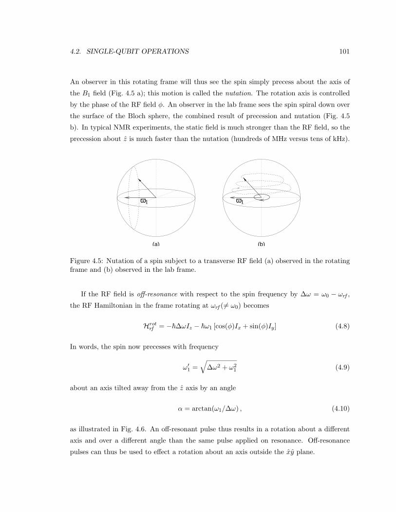
4.2. SINGLE-QUBIT OPERATIONS 101
An observer in this rotating frame will thus see the spin simply precess about the axis of
the B1 field (Fig. 4.5 a); this motion is called the nutation. The rotation axis is controlled
by the phase of the RF field φ. An observer in the lab frame sees the spin spiral down over
the surface of the Bloch sphere, the combined result of precession and nutation (Fig. 4.5
b). In typical NMR experiments, the static field is much stronger than the RF field, so the
precession about z is much faster than the nutation (hundreds of MHz versus tens of kHz).
(a) (b)
ω1ω1
Figure 4.5: Nutation of a spin subject to a transverse RF field (a) observed in the rotatingframe and (b) observed in the lab frame.
If the RF field is off-resonance with respect to the spin frequency by ∆ω = ω0 − ωrf ,
the RF Hamiltonian in the frame rotating at ωrf (6= ω0) becomes
Hrotrf = −~∆ωIz − ~ω1 [cos(φ)Ix + sin(φ)Iy] (4.8)
In words, the spin now precesses with frequency
ω′1 =√
∆ω2 + ω21 (4.9)
about an axis tilted away from the z axis by an angle
α = arctan(ω1/∆ω) , (4.10)
as illustrated in Fig. 4.6. An off-resonant pulse thus results in a rotation about a different
axis and over a different angle than the same pulse applied on resonance. Off-resonance
pulses can thus be used to effect a rotation about an axis outside the xy plane.

102 CHAPTER 4. LIQUID-STATE NMR QUANTUM COMPUTING
ω1
∆ω ω1α
Figure 4.6: Axis of rotation (in the rotating frame) during an off-resonant radio-frequencypulse.
RF pulses
A resonant RF field gated on for a duration pw, nutates a spin in the rotating frame over
an angle
θ = γ B1 pw . (4.11)
The parameter pw is called the pulse width or pulse length.
Thus, a properly timed and calibrated RF pulse with the right phase can perform a
rotation about x of 90, which we will denote Rx(90) (see Eq. 2.45) or for short X. A similar
pulse but twice as long realizes a Rx(180) rotation, written for short as X2. By changing
the phase of the RF by 90, we can similarly implement Y and Y 2 pulses. Changing the
phase another 90 gives a negative rotation about x, denoted Rx(−90) or X, and so forth.
We point out that only the relative phase between pulses applied to the same spin
matters. As soon as we send one pulse on any given spin, the phase of that pulse sets the
phase reference of the corresponding rotating frame for the remainder of the pulse sequence.
Quantum picture
The description of single-spin rotations has been purely classical so far, and in fact it does
not need quantum mechanics at all. For example, a bar magnet with angular momentum
responds in exactly the same way to magnetic fields as does a nuclear spin. However, the
quantum nature of spins, and qubits in general, unmistakably emerges as soon as two or
more spins are involved (section 2.1.1).
Underlying the classical Bloch sphere picture is the evolution of a two-level quantum
mechanical system. An RF field induces transitions between the ground and excited state of
the qubit (Fig. 4.1). After applying an RF pulse, a spin initially in the ground state will upon
measurement be found in the excited state with probability sin2(ω1pw/2). The projection

4.2. SINGLE-QUBIT OPERATIONS 103
on the z axis of the Bloch sphere oscillates with pw as cos(ω1pw). These oscillations are
known as Rabi oscillations, and ω1/2π is the Rabi frequency, with typical values of a few
hundred Hz to a few hundred kHz.
4.2.2 Rotations about the z axis
We recall from Eq. 2.53 that the ability to implement arbitrary rotations about x and
y is sufficient for performing arbitrary single-qubit rotations. For example, two ways to
implement a Z rotation using composite X and Y pulses are
Z = XY X = Y XY , (4.12)
where time goes from right to left, as always for concatenated unitary operations (see sec-
tion 2.2.3). We have used this technique in our first few experiments (sections 5.3-5.5).
However, there are two alternative and more convenient ways to implement Z rotations.
The first approach takes place at the pulse sequence design level. The goal is to move
down all the Z rotations to the very end or the beginning of the pulse sequence. For
example, using Eq. 4.12, we can move a Z rotation past a X or Y rotation,
ZY = XY XY = XZ . (4.13)
Since Z rotations commute with the Hamiltonian of nuclear spins in liquid solution, they
can be moved across time evolution intervals as well. Once all Z rotations are gathered
at the end of the pulse sequence, we only need to execute the net remaining Z rotation
for each spin. Z rotations moved to the start of the sequence have no effect as the initial
state is diagonal (see section 4.4), so they don’t need to be implemented altogether. This
approach was used in the experiment of section 5.7.
The second approach has the same effect, but the experimental procedure is different.
It makes use of an artificial software rotating frame, on top of the hardware rotating frame
provided by a reference oscillator. A Z rotation is implemented simply by shifting the
software reference frame by 90. Subsequent X and Y pulses are then executed with respect
to the new reference frame (e.g. X in the new frame corresonds to Y in the old frame, and
so forth), and the receiver phase is also set with respect to the new software frame. We have
used this procedure in our latest experiments (sections 5.8- 5.10), as it is by far the easiest
to use once the software for the artificial reference frame is written. Since the Z rotations
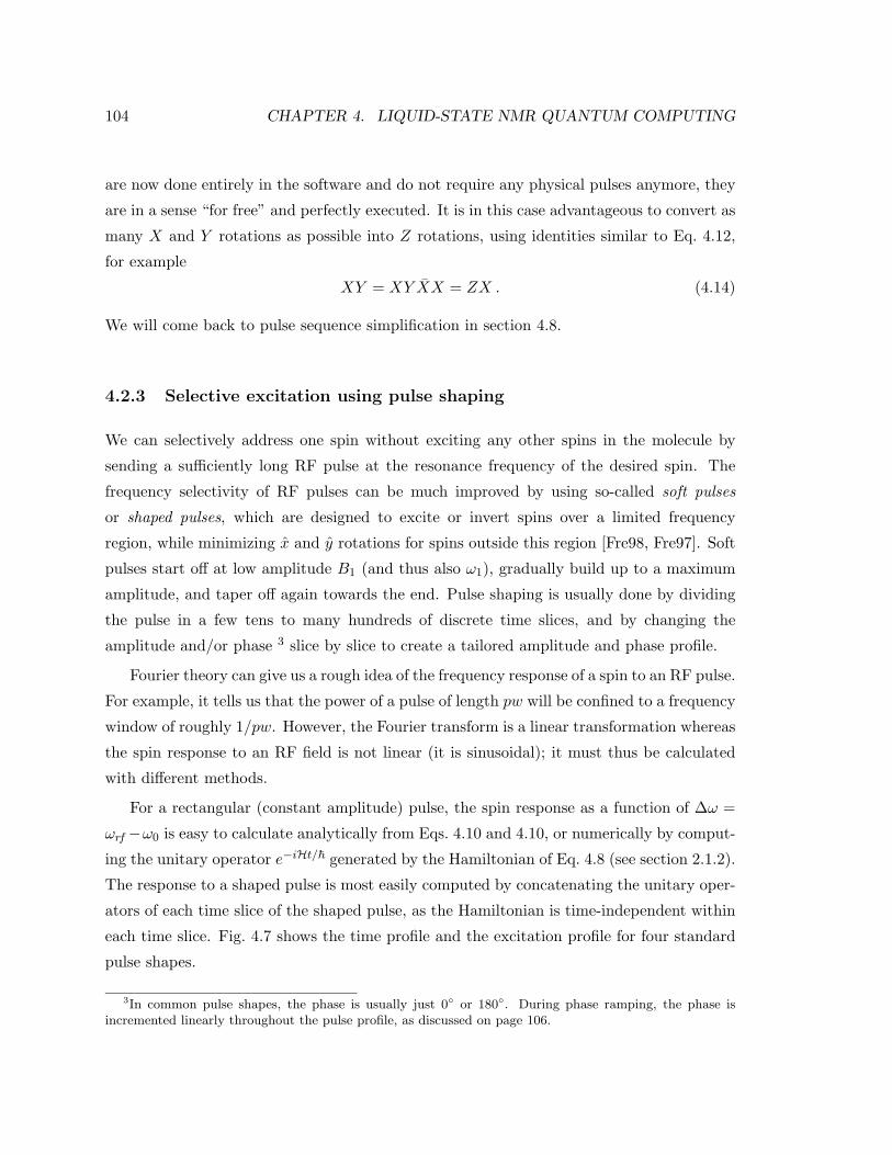
104 CHAPTER 4. LIQUID-STATE NMR QUANTUM COMPUTING
are now done entirely in the software and do not require any physical pulses anymore, they
are in a sense “for free” and perfectly executed. It is in this case advantageous to convert as
many X and Y rotations as possible into Z rotations, using identities similar to Eq. 4.12,
for example
XY = XY XX = ZX . (4.14)
We will come back to pulse sequence simplification in section 4.8.
4.2.3 Selective excitation using pulse shaping
We can selectively address one spin without exciting any other spins in the molecule by
sending a sufficiently long RF pulse at the resonance frequency of the desired spin. The
frequency selectivity of RF pulses can be much improved by using so-called soft pulses
or shaped pulses, which are designed to excite or invert spins over a limited frequency
region, while minimizing x and y rotations for spins outside this region [Fre98, Fre97]. Soft
pulses start off at low amplitude B1 (and thus also ω1), gradually build up to a maximum
amplitude, and taper off again towards the end. Pulse shaping is usually done by dividing
the pulse in a few tens to many hundreds of discrete time slices, and by changing the
amplitude and/or phase 3 slice by slice to create a tailored amplitude and phase profile.
Fourier theory can give us a rough idea of the frequency response of a spin to an RF pulse.
For example, it tells us that the power of a pulse of length pw will be confined to a frequency
window of roughly 1/pw. However, the Fourier transform is a linear transformation whereas
the spin response to an RF field is not linear (it is sinusoidal); it must thus be calculated
with different methods.
For a rectangular (constant amplitude) pulse, the spin response as a function of ∆ω =
ωrf −ω0 is easy to calculate analytically from Eqs. 4.10 and 4.10, or numerically by comput-
ing the unitary operator e−iHt/~ generated by the Hamiltonian of Eq. 4.8 (see section 2.1.2).
The response to a shaped pulse is most easily computed by concatenating the unitary oper-
ators of each time slice of the shaped pulse, as the Hamiltonian is time-independent within
each time slice. Fig. 4.7 shows the time profile and the excitation profile for four standard
pulse shapes.
3In common pulse shapes, the phase is usually just 0 or 180. During phase ramping, the phase isincremented linearly throughout the pulse profile, as discussed on page 106.
4.2. SINGLE-QUBIT OPERATIONS 105
Rec
tang
ular
0 200 400 600 800 1000
−1
0
1
2
3
4
5
6
Time [µs]
ω1 [k
Hz]
−6000 −4000 −2000 0 2000 4000 6000−1
−0.5
0
0.5
1
∆ ω / (2π) [Hz]
Nor
mal
ized
am
plitu
de
Z XY
Gau
ssia
n
0 200 400 600 800 1000
−1
0
1
2
3
4
5
6
Time [µs]
ω1 [k
Hz]
−6000 −4000 −2000 0 2000 4000 6000−1
−0.5
0
0.5
1
∆ ω / (2π) [Hz]
Nor
mal
ized
am
plitu
de
Z XY
Her
mit
e18
0
0 200 400 600 800 1000
−1
0
1
2
3
4
5
6
Time [µs]
ω1 [k
Hz]
−6000 −4000 −2000 0 2000 4000 6000−1
−0.5
0
0.5
1
∆ ω / (2π) [Hz]
Nor
mal
ized
am
plitu
de
Z XY
reburp
0 200 400 600 800 1000
−1
0
1
2
3
4
5
6
Time [µs]
ω1 [k
Hz]
−6000 −4000 −2000 0 2000 4000 6000−1
−0.5
0
0.5
1
∆ ω / (2π) [Hz]
Nor
mal
ized
am
plitu
de
Z XY
Figure 4.7: (Left) Time profile and (Right) frequency excitation profiles (displaying the zand xy component of the Bloch vector after a pulse when the Bloch vector is along +zbefore the pulse) for four relevant pulse shapes.

106 CHAPTER 4. LIQUID-STATE NMR QUANTUM COMPUTING
Pulse shape design
The properties relevant for choosing a pulse shape are:
• selectivity: product of excitation bandwidth and pulse length (lower is more selective),
• transition range: the width of the transition region between the selected and unse-
lected frequency region,
• power: the peak power required for a given pulse length (low is less demanding),
• self-refocusing behavior (see section 4.2.4): degree to which the J couplings between
the selected spin and other spins are refocused (the signature for self-refocusing be-
havior is a flat top in the excitation profile),
• robustness: whether the spin response is very sensitive to experimental imperfections
such as RF field inhomogeneities and calibration errors,
• universality: whether the pulse performs the correct rotation for arbitrary input states
or only for specific input states.
Figure 4.7 strikingly illustrates the difference in performance between different pulse shapes.
Table 4.2 summarizes these properties for a selection of important pulse shapes. All the
pulses in the table are universal pulses; quantum computations must work for any input
state so we cannot compromise on universality.4 Obviously, no single pulse shape optimizes
for all properties simultaneously, so pulse shape design consists of finding the optimal trade
off for the desired application. For our experiments, we have been selected molecules with
large chemical shifts, so sharp transition regions are not so important. Furthermore, the
probes and spectrometer can deal with relatively high powers. The crucial parameters are
the effect of coupling during the pulses, the selectivity (short, selective pulses minimize
relaxation) and to some extent the robustness.
Phase ramping
Excitation at a frequency which differs from the RF carrier frequency ωrf by ∆ω, is made
possible by linearly incrementing the phase of the pulse during the application of the pulse,4Strictly speaking, one could use non-universal pulses in the early stages of certain algorithms, or during
the state preparation sequences, but we have never done this.

4.2. SINGLE-QUBIT OPERATIONS 107
selec- transition self- robust-tivity range power refocusing ness
Rectangular poor very wide minimal no goodGauss 90 [BFF+84] excellent wide low fair goodGauss 180 [BFF+84] excellent wide low fair goodHrm 90 [War84] moderate moderate average good fairHrm 180 [War84] good moderate average very good fairuburp 90 [GF91] poor narrow high excellent poorreburp 180 [GF91] poor narrow high excellent poorav 90 [AV93] fair moderate average good fair
Table 4.2: Properties of relevant pulse shapes
at a rate δφ/δt = ∆ω. The result of this procedure, known as phase-ramping [Pat91], is
that the frequency of the output signal of the phase shifter is δφ/δt higher than ωrf , the
frequency at the input of the phase shifter. This is expressed by replacing Eq. 4.6 by
Hrf = ~ω1
cos[ωrf t+
(φ0 +
δφ
δtt
)]Ix + sin
[ωrf t+
(φ0 +
δφ
δtt
)]Iy
= ~ω1
cos[(ωrf +
δφ
δt
)t+ φ0
]Ix + sin
[(ωrf +
δφ
δt
)t+ φ0
]Iy
. (4.15)
In practice, the continuous phase ramp is approximated by discrete steps ∆φ from one time
slice of duration ∆t to the next, such that ∆φ/∆t = δφ/δt. If ∆t is short enough such that
∆φ is only a few degrees to about 10 degrees, this is a good approximation of a continuous
phase ramp.
Excitation at multiple frequencies simultaneously via a single pulse can be accomplished
by an extension of phase ramping. Within each time slice, the amplitude and phase of each
pulse describe a vector. In order to merge several pulses into a single pulse, it suffices to
take the vector sum of all the original pulses within each slice and use this sum to describe
the corresponding time slice of the combined pulse.
4.2.4 Single pulses - artefacts and solutions
Bloch-Siegert shifts
The presence of RF irradiation during pulses causes a shift ∆ωBS in the precession frequency
of spins at frequencies well outside the excitation frequency window [EB90]. This effect has
108 CHAPTER 4. LIQUID-STATE NMR QUANTUM COMPUTING
become known as a transient (generalized) Bloch-Siegert shift 5; at a deeper level, the
acquired phase can be understood as an instance of Berry’s phase [Ber84]. The magnitude
of ∆ωBS is approximately ω21/2(ωrf − ω0) (for ω1 ωrf − ω0), where ω0 is the Larmor
frequency in the absence of an RF field. The frequency shifts can easily reach several
hundred Hz and the direction of the shift is always away from the frequency of the RF field.
Each spin thus accumulates a spurious phase shift during RF pulses applied to spins
at nearby frequencies. Since ω1 varies over time for shaped pulses, the Bloch-Siegert shift
generally varies throughout the pulse, but the cumulative phase shifts can be easily com-
puted in advance for each possible spin-pulse combination, if all the frequency separations,
pulse shapes and pulse lengths are known. The unintended phase shifts Rz(θ) can then be
compensated for during the execution of a pulse sequence by inserting appropriate Rz(−θ).This is easy to do, especially if software reference frames are used (section 4.2.2).
Coupled evolution during pulses
Spins within the same molecule interact with each other via the J coupling (Eq. 4.4). This
interaction forms the basis for two-qubit gates (section 4.3), but the spin-spin interactions
cannot be turned off and are thus also active during the RF pulses, which are intended
to be just single-qubit transformations. For short pulses at high power, J is very small
compared to ω1 so the coupled evolution which takes place during the pulses is negligible.
However, for soft pulses, ω1 is often of the same order of magnitude as J , and in this case
the coupling terms strongly affect the intended nutation, in a way similar to off-resonance
effects (Fig. 4.6): coupling to another spin shifts the spin frequency to ω0 ± J/2, so a pulse
sent at ω0 hits the spin off-resonance by ±J/2.
Fortunately, specialized pulse shapes exist which minimize the effect of coupling during
the pulses (see Table 4.2). Such self-refocusing pulses [GF91] take a spin over a complicated
trajectory in the Bloch sphere, in such a way that the net effect of couplings between the
selected and non-selected spins is reduced. It is as if those couplings are only in part or
even not at all active during the pulse (couplings between pairs of non-selected spins will
still be fully active). Although the self-refocusing behavior of certain shaped pulses can
be intuitively explained to some degree, many actual pulse shapes have been the result of
5The original paper by Bloch and Siegert [BS40] refers to the frequency shift produced by the counter-rotating RF field (see page 100), but the term Bloch-Siegert shift has been used in a generalized sense inthe NMR community.
4.2. SINGLE-QUBIT OPERATIONS 109
numerical optimizations. Table 4.2 summarizes how effective several common pulse shapes
are at refocusing the J couplings. A general observation is that it is relatively easy to make
180 pulses self-refocusing, but much harder for 90 pulses.
Complementary to the use of self-refocusing pulses, undesired coupled evolution that
still takes place during a pulse can be (in part) unwound at a different time in the pulse
sequence via a “negative” time evolution (section 4.3.1). A complication in unwinding the
coupled evolution is that Hrf and HJ do not commute; this implies that a real pulse can-
not be perfectly decomposed into an idealized pulse (no coupling present) followed and/or
preceeded by a time interval of coupled evolution.
Nevertheless, we found that the coupled evolution is reversed quite well by a negative
time interval both before and after the pulse,
e+iHJ pw τ/~e−i(Hrf+HJ ) pw /~e+iHJ pw τ/~ ≈ e−iHrf pw /~ , (4.16)
where τ is chosen in each equation such that the approximations are as good as possible
according to some matrix distance (we have used the 2-norm distance measure). A negative
time interval only before or after the pulse,
e+iHJ pw τ/~e−i(Hrf+HJ ) pw /~ ≈ e−iHrf pw /~ ≈ e−i(Hrf+HJ ) pw /~e+iHJ ) pw τ/~ , (4.17)
is much less effective. This is can be seen from Table 4.3, which we will now discuss.
For Gaussian 90 pulses, the J1i evolution, which doesn’t commute with X1, is unwound
much better by two symmetrically placed negative time evolution intervals of duration pwτ
than by a single τ (we will from now on leave pw implicit; τ will be in units of pw throughout)
before or after the pulse. Furthermore, while evolution under Jij (i, j 6= 1) commutes with
a pulse on spin 1 and can thus be perfectly reversed, the optimal values of τ to unwind J1i
and Jjk evolution lie much closer together if the τ ’s are placed symmetrically.
Hermite shaped 180 pulses are self-refocusing, so J1i is not active during the pulse and
need not be reversed. In the asymmetric scheme with only a single τ either before or after
the pulse, τ must thus be 0 such that no J1i evolution is introduced. However, in order
to unwind Jij , we need τ to be 1. We can thus not take care of both J1i and Jij in the
asymmetric scheme. In contrast, a symmetric pair of intervals τ separated by a 180 pulse
on spin 1 gives net zero J1i evolution for any value of τ . We can thus set τ to the optimal
value for unwinding Jjk and obtain an excellent net single-qubit 180 rotation.

110 CHAPTER 4. LIQUID-STATE NMR QUANTUM COMPUTING
gauss90 X1τ τX1τ
J1i fair, τ ≈ 0.6 excellent, τ ≈ 0.57Jij perfect, τ = 1 perfect, τ = 0.5
J1i, Jij fair, (0.6 <)τ < 1 very good, 0.5 < τ < 0.57
hrm180 X1τ τX1τ
J1i excellent, τ = 0 excellent, ∀τJij perfect, τ = 1 perfect, τ = 0.5
J1i, Jij poor, 0 < τ < 1 excellent, τ = 0.5
Table 4.3: Comparison of the degree to which J-coupled evolution during a single pulse onspin 1 is unwound via asymmetric versus symmetric negative time intervals τ (expressed asa fraction of the duration of pw), for various coupling scenarios. The optimal τ is indicatedin each case.
In practice, we have used the symmetrized decomposition of Eq. 4.16 in order to obtain
a first order improvement in the unitary evolution. Further fine-tuning can be done if
different negative evolution times are allowed to unwind different coupling terms. Higher-
order corrections are in principle possible because the undesired evolution is known and can
be fully characterized, although such a scheme would be substantially more complicated
to implement. Also, with the degree of control in current implementations, it is unclear if
such higher order corrections would be effective. Finally, if the input state is diagonal, as
is the case in many input state preparation pulse sequences, couplings that do not involve
the selected spin (e.g. J23 during X1 pulses) have no effect, and need not be unwound. In
this case, τ should be optimized to refocus just the J1i couplings.
It is clear that properly controlling non-commuting terms in the Hamiltonian will be
a recurring challenge for virtually any proposed quantum computer implementation. We
believe that a general (as opposed to an ad-hoc) and practical method for removing the effect
of select terms in the Hamiltonian constitutes an important and interesting open problem.
4.2.5 Simultaneous pulses - artefacts and solutions
Simultaneous pulses, as opposed to consecutive pulses, are desirable for quantum compu-
tation because they help keep the pulse sequence within the coherence time. However, the
effects of Bloch-Siegert shifts, discussed in the previous section for single pulses, are aggra-
vated during simultaneous pulses. The effect of J couplings during simultaneous pulses also

4.2. SINGLE-QUBIT OPERATIONS 111
deserves a separate discussion.
Bloch-Siegert shifts
The Bloch-Siegert shifts introduced in the previous section result in additional problems
during simultaneous pulses applied to two or more spins at nearby frequencies. If we apply
spin-selective pulses simultaneously to two spins 1 and 2 with resonance frequencies ω10 and
ω20 (say ω1
0 < ω20), the pulse at ω1
0 temporarily shifts the frequency of spin 2 to ω20 + ∆ωBS .
As a result, the pulse on spin 2, which is still applied at ω20, will be off-resonance by an
amount −∆ωBS . Analogously, the pulse at ω10 is now off the resonance of spin 1 by ∆ωBS .
The resulting rotations of the spins deviate significantly from the intended rotations.
Fig. 4.8 shows the simulated inversion profiles for a spin subject to two simultaneous
Hermite 180 pulses separated by 3273 Hz. The centers of the inversion profiles have
shifted away from the intended frequencies and the inversion is incomplete, which can be
seen most clearly from the substantial residual xy-magnetization (> 30%) over the whole
region intended to be inverted. Note that since the frequencies of the applied pulses are
off the spin resonance frequencies, perfect rotations cannot be achieved no matter what
tip angle is chosen. In practice, simultaneous soft pulses at nearby frequencies have been
avoided in NMR [LKF99] or the poor quality of the spin rotations was accepted.
−6000 −4000 −2000 0 2000 4000 6000−1
−0.5
0
0.5
1
spin frequency [Hz]
ampl
itude
Z XY
Figure 4.8: Simulation of the amplitude of the z and xy component of the magnetizationof a spin as a function of its frequency. The spin starts out along +z and is subject totwo simultaneous Hermitian shaped pulses with carrier frequencies at 0 Hz and 3273 Hz(vertical dashed lines), with a calibrated pulse length of 2650µs (ideally 180).
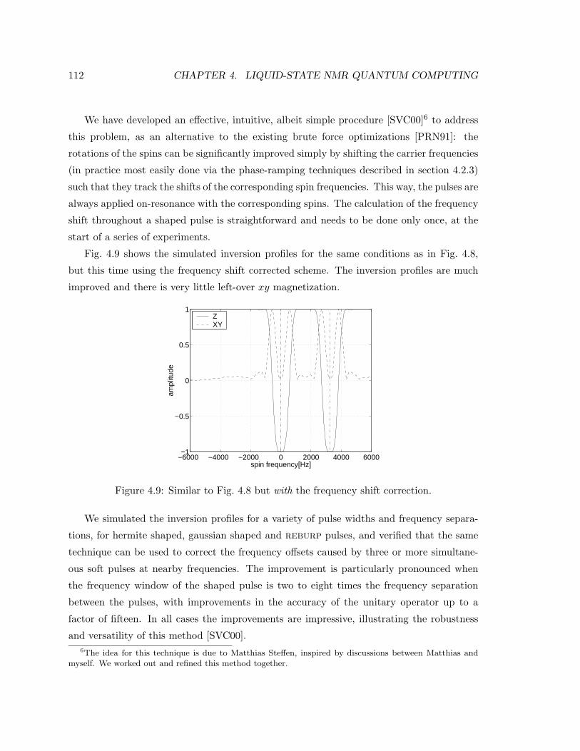
112 CHAPTER 4. LIQUID-STATE NMR QUANTUM COMPUTING
We have developed an effective, intuitive, albeit simple procedure [SVC00]6 to address
this problem, as an alternative to the existing brute force optimizations [PRN91]: the
rotations of the spins can be significantly improved simply by shifting the carrier frequencies
(in practice most easily done via the phase-ramping techniques described in section 4.2.3)
such that they track the shifts of the corresponding spin frequencies. This way, the pulses are
always applied on-resonance with the corresponding spins. The calculation of the frequency
shift throughout a shaped pulse is straightforward and needs to be done only once, at the
start of a series of experiments.
Fig. 4.9 shows the simulated inversion profiles for the same conditions as in Fig. 4.8,
but this time using the frequency shift corrected scheme. The inversion profiles are much
improved and there is very little left-over xy magnetization.
−6000 −4000 −2000 0 2000 4000 6000−1
−0.5
0
0.5
1
spin frequency[Hz]
ampl
itude
Z XY
Figure 4.9: Similar to Fig. 4.8 but with the frequency shift correction.
We simulated the inversion profiles for a variety of pulse widths and frequency separa-
tions, for hermite shaped, gaussian shaped and reburp pulses, and verified that the same
technique can be used to correct the frequency offsets caused by three or more simultane-
ous soft pulses at nearby frequencies. The improvement is particularly pronounced when
the frequency window of the shaped pulse is two to eight times the frequency separation
between the pulses, with improvements in the accuracy of the unitary operator up to a
factor of fifteen. In all cases the improvements are impressive, illustrating the robustness
and versatility of this method [SVC00].6The idea for this technique is due to Matthias Steffen, inspired by discussions between Matthias and
myself. We worked out and refined this method together.

4.2. SINGLE-QUBIT OPERATIONS 113
We have experimentally confirmed the improvements predicted by the simulations, and
used this technique in the experiments of sections 5.9 and 5.10.
Coupled evolution during pulses
The evolution of two coupled spins which are pulsed simultaneouly leads to multiple-
quantum coherences, even if the pulses are self-refocusing, because the interaction between
the two pulses disturbs the self-refocusing behavior [KF95]. Can we compensate for this
coupled evolution using negative time evolution before and after? Or is it better to send
the pulses back to back? Table 4.4 reviews these questions for the case of gaussian 90 and
Hermite 180 pulses.
The back to back Gaussian 90 pulses very poorly unwind any J ’s involving one or both
selected spins. Using simultaneous pulses and symmetrically placed τ ’s, J12 is still not very
well reversed, but all the J1i and J2i (i 6= 1, 2) are unwound very well. Jij (i, j 6= 1, 2)
always commutes with pulses on spins 1 and 2, and can thus be perfectly unwound, with an
optimal value of τ close to the optimal value for reversing the evolution under other J ’s. In
the end, the achieved unitary evolution is quite good when using simultaneous pulses with
negative evolution before and after, as long as J12 is not too strong.
Because Hermite shaped 180 pulses are self-refocusing, J12 is not active during the back
to back pulses and need not be reversed; however, all the other couplings are very poorly
unwound when using back to back pulses. During two simultaneous pulses, J12 is almost
fully active, but can be unwound quite well; the J1i and J2i can be reversed very well too.
As always, Jij commutes with pulses on spins 1 and 2, and can thus be perfectly unwound.
If the negative evolution is arranged symmetrically (and only then), the optimal values of τ
for unwinding the evolution under the respective couplings are all approximately the same,
resulting in a very good unitary transformation for simultaneous pulses with symmetric
unwinding.
The general conclusion is that it is much better to send the two pulses simultaneously
than back to back. Furthermore, as was the case for single pulses, it is by far better to have
negative evolution both before and after the pulses.
Even with symmetrically placed negative time intervals and using simultaneous pulses,
the coupled evolution which takes place during the pulses is often (depending on the value
of the respective Jij) not unwound to the same degree as in the case of single pulses, and

114 CHAPTER 4. LIQUID-STATE NMR QUANTUM COMPUTING
gauss90 τX1X2τ τX1,2τ X1,2τ
J12 poor, τ ≈ 0.57 fair, τ ≈ 0.5 poor, τ ≈ 0.9J1i, J2i poor, τ ≈ 1.06 excellent, τ ≈ 0.57 fair, τ =≈ 0.57
J12, J1i, J2i poor, 0.57 < τ < 1.15 good, (0.5 <)τ < 0.57 poor, 0.45 < τ < 0.65Jij perfect, τ = 1 perfect, τ = 0.5 perfect, τ = 1
hrm180 τX1X2τ τX1,2τ X1,2τ
J12 excellent, τ = 0 good, τ ≈ 0.45 good, τ ≈ 0.9J1i, J2i poor, τ > 0 excellent, ∀τ excellent, τ = 0
J12, J1j , J2i poor, τ = 0 very good, τ ≈ 0.45 poor, 0 < τ < 0.9Jij perfect, τ = 1 perfect, τ = 0.5 perfect, τ = 1
Table 4.4: Comparison of the degree to which J-coupled evolution during two pulses isunwound for three scenario’s: (1) two pulses back to back preceeded and followed by negativeevolution, (2) two simultaneous pulses preceeded and followed by negative evolution, and forcomparison (3) two simultaneous pulses only followed by negative evolution. The optimalτ is indicated in each case.
τX12τX2τ may in some cases give better results than simultaneous pulses. However, im-
plementing the negative time evolution in between the two pulses makes the pulse sequence
much longer.
In the experiments, we have also used three simultaneous pulses. Similar arguments for
the compensation of J-coupled evolution as those we made for two simultaneous pulses,
hold for three or more simultaneous pulses.
4.3 Two-qubit operations
4.3.1 The controlled-not in a two-spin system
The basis for two-qubit gates in NMR is the pairwise interaction between spins in the same
molecule, described in section 4.1.2. The most natural two-qubit gate between nuclear
spins in a molecule is therefore an evolution under the coupling Hamiltonian of Eq. 4.4 for
a duration t,
UJ(t) = exp[−i2πJI1z I
2z t] =
e−iπJt/2 0 0 0
0 e+iπJt/2 0 0
0 0 e+iπJt/2 0
0 0 0 e−iπJt/2
. (4.18)
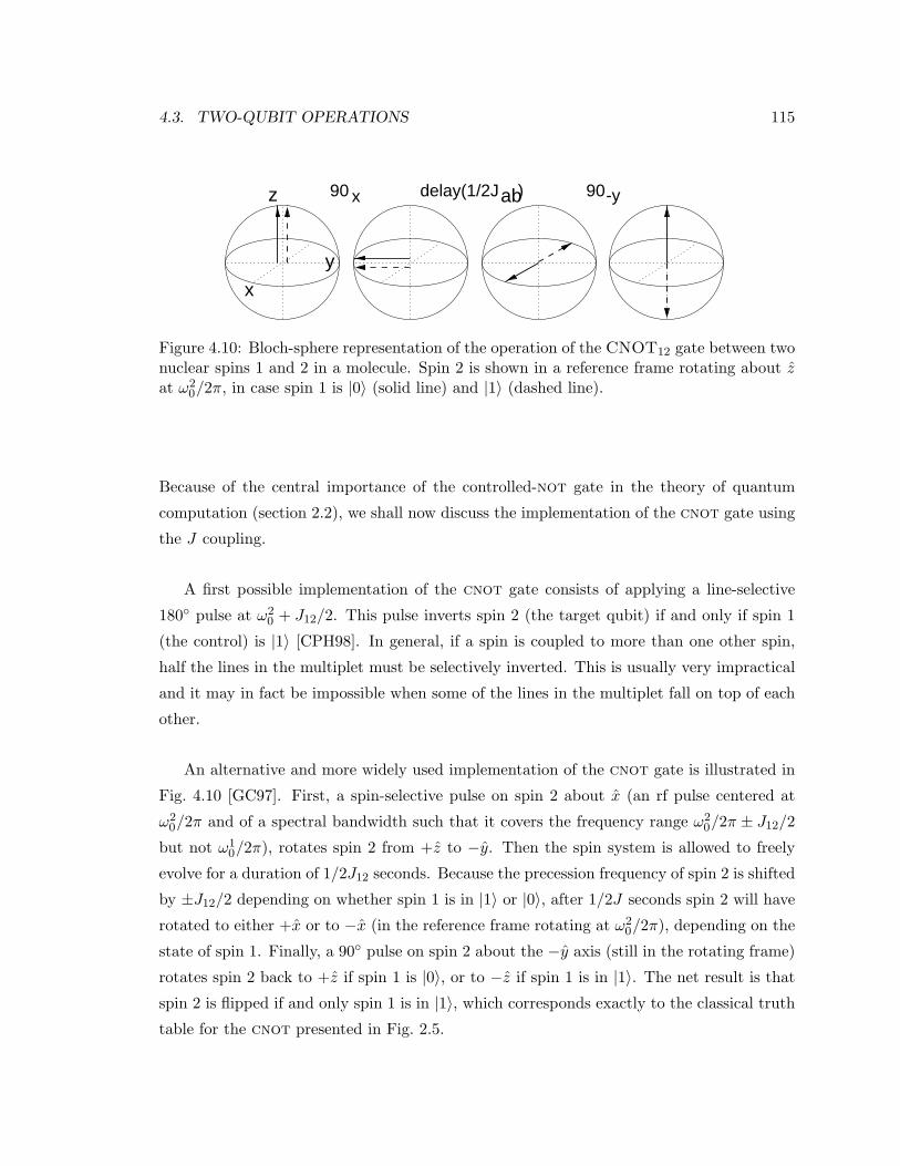
4.3. TWO-QUBIT OPERATIONS 115
x
y
z 90 x 90-yabdelay(1/2J )
Figure 4.10: Bloch-sphere representation of the operation of the CNOT12 gate between twonuclear spins 1 and 2 in a molecule. Spin 2 is shown in a reference frame rotating about zat ω2
0/2π, in case spin 1 is |0〉 (solid line) and |1〉 (dashed line).
Because of the central importance of the controlled-not gate in the theory of quantum
computation (section 2.2), we shall now discuss the implementation of the cnot gate using
the J coupling.
A first possible implementation of the cnot gate consists of applying a line-selective
180 pulse at ω20 + J12/2. This pulse inverts spin 2 (the target qubit) if and only if spin 1
(the control) is |1〉 [CPH98]. In general, if a spin is coupled to more than one other spin,
half the lines in the multiplet must be selectively inverted. This is usually very impractical
and it may in fact be impossible when some of the lines in the multiplet fall on top of each
other.
An alternative and more widely used implementation of the cnot gate is illustrated in
Fig. 4.10 [GC97]. First, a spin-selective pulse on spin 2 about x (an rf pulse centered at
ω20/2π and of a spectral bandwidth such that it covers the frequency range ω2
0/2π ± J12/2
but not ω10/2π), rotates spin 2 from +z to −y. Then the spin system is allowed to freely
evolve for a duration of 1/2J12 seconds. Because the precession frequency of spin 2 is shifted
by ±J12/2 depending on whether spin 1 is in |1〉 or |0〉, after 1/2J seconds spin 2 will have
rotated to either +x or to −x (in the reference frame rotating at ω20/2π), depending on the
state of spin 1. Finally, a 90 pulse on spin 2 about the −y axis (still in the rotating frame)
rotates spin 2 back to +z if spin 1 is |0〉, or to −z if spin 1 is in |1〉. The net result is that
spin 2 is flipped if and only spin 1 is in |1〉, which corresponds exactly to the classical truth
table for the cnot presented in Fig. 2.5.

116 CHAPTER 4. LIQUID-STATE NMR QUANTUM COMPUTING
However, the sequence of Fig. 4.10 actually implements the unitary transformation
X2 UJ(1/2J)Y2 = Ucnot12 =
1 0 0 0
0 i 0 0
0 0 0 −i0 0 1 0
, (4.19)
which is similar to but different from Ucnot of Eq. 2.51. An additional phase shift on both
spins is needed in order to obtain Ucnot exactly:
Z1Z2X2 UJ(1/2J)Y2 = Ucnot12 =
1 0 0 0
0 1 0 0
0 0 0 1
0 0 1 0
. (4.20)
4.3.2 Refocusing select J couplings
The coupling terms in the Hamiltonian of nuclear spins in a molecule are given by nature
and cannot be turned off. Therefore, in order to implement a cnotij in a molecule with
n coupled spins, we need a means to effectively deactivate all couplings except Jij . This is
done in NMR by refocusing the undesired coupled evolutions via a sequence of 180 pulses,
in a similar way as is done in spin-echo experiments.
Fig. 4.11 pictorially shows how refocusing pulses can neutralize the J coupling between
two spins. In (a), the evolution of spin 1 which takes place in the first time interval is
reversed in the second time interval, due to the 180 pulse on spin 2. In (b), spin 1 continues
to evolve in the same direction the whole time, but still comes back to its initial position
thanks to the 180 pulse on spin 1. The second 180 pulse is needed to ensure that both
spins return to their initial state regardless of the initial state. We note that if refocusing
pulses are sent on both spins simultaneously, the coupling is active again.
Mathematically, we can see how refocusing of J couplings works via
X21 UJ(τ)X2
1 = UJ(−τ) = X22 UJ(τ)X2
2 , (4.21)
which leads to
X21 UJ(τ)X2
1 UJ(τ) = I = X22 UJ(τ)X2
2 UJ(τ) (4.22)
for all values of τ .

4.3. TWO-QUBIT OPERATIONS 117
(a)
(b)
x
y
z
x
y
z
τ τ
ττ
delay( ) delay( )
delay( )delay( )
1802y 1802
y
1801y180y
1
Figure 4.11: Bloch-sphere representation of the operation of a simple scheme to refocus thecoupling between two coupled spins. The diagram shows the evolution of spin 1 (in therotating frame) initially along y, when spin 1 is in |0〉 (solid) or in |1〉 (dashed).
Fig. 4.12 shows a refocusing scheme which preserves the effect of the J12 coupling in a
four spin system, while effectively inactivating all the other couplings. The underlying idea
is that a coupling between spins i and j acts “forward” during intervals where both spins
have the same sign in the diagram, and acts “in reverse” whenever the spins have opposite
signs. Whenever a coupling acts forward and in reverse for the same duration over the
course of a refocusing scheme, it has no net effect. If the forward and reverse evolutions are
not balanced in duration, a net coupled evolution takes place corresponding to the excess
forward or reverse evolution.
Systematic methods for designing refocusing schemes for multi-spin systems have been
developed specifically for the purpose of quantum computing. The most compact scheme
is based on Hadamard matrices [LCYY00, JK99], but this is also the experimentally most
demanding, as it requires that many spins be pulsed simultaneously. On the other extreme
are schemes without any simultaneous pulses [LBCF99], but which take significantly longer.
Finally, we point out that refocusing schemes can be considerably simplified if we know
that certain spins are along the z axis, because the J coupling does not affect spins along
the z axis. This is a common situation in the early stages of a quantum computations.
Fig. 4.13 gives such a simplified refocusing scheme for five coupled spins.

118 CHAPTER 4. LIQUID-STATE NMR QUANTUM COMPUTING
+ + + +
+ + + + + + + +
+ + + + - - --
- - --
+ + + +
+ + + +
3
4
2
1
Figure 4.12: Refocusing scheme for a four spin system. J12 is active the whole time but theeffect of the other Jij is neutralized. The interval is divided into slices of equal duration,and the “+” and “-” signs indicate whether a spin is still in its original position, or upsidedown. At the interface of certain time slices, 180 pulses (assumed to be instantaneous, andshown as black retangles) are sent on one or more spins; the pulsed spins transition from +to − or back.
2 + -
3 + +
4 + +
+ +5
1 + -
Figure 4.13: Simplified refocusing scheme for five spins, which can be used if we know inadvance that spins 3, 4 and 5 are along ±z. J12 is active, but J13, J14, J15, J23, J24, J25
are inactive. The remaining couplings are active but have no effect given the initial state.
Negative time evolution
It is sometimes necessary to implement a unitary transformation which corresponds to a
free evolution under certain couplings for a negative time. From the preceding paragraphs,
we see that this can be achieved using a refocusing sequence where the desired couplings
evolve in reverse for a longer time than they act forward.
Starting from an existing refocusing scheme, negative evolutions can thus be obtained
simply by reducing the appropriate delay times. Of course, the effective negative time
evolution obtained in this way cannot be longer than the original delay times. If longer
negative delay times are needed, we can increase the remaining delay times in order to
increase the imbalance between forward and reverse evolutions for the desired couplings.
If there is no refocusing sequence already in place which can be changed, realizing
4.3. TWO-QUBIT OPERATIONS 119
negative time evolution under certain couplings requires an additional refocusing sequence.
This is obviously to be avoided if possible.
Coupling network considerata
For systems with more than two spins, two complications arise when performing two-qubit
gates. They are illustrated by the two extreme coupling networks in Fig. 3.1 (a) and (b).
First, if two spins are not directly coupled to each other, a cnot between these two spins
must be done using intermediary spins (see section 3.1.2, p. 60) [CKH+00]. Second, if every
spin is coupled to every other spin (this is possible only in relatively small molecules), the
pulse sequence of Fig. 4.10 must be supplemented by a complex refocusing scheme which
selects only the desired coupling.
Clearly, both scenarios are associated with a considerable overhead. It is important to
note that this overhead is only polynomial (at most quadratic) in the number of qubits. A
cnot between any two qubits along a chain of n spins with just nearest-neighbour couplings
takes at most 2(n− 2) swap operations, and a Hadamard based refocusing scheme between
n fully coupled spins takes at most n time segments and no more than n 180 pulses per
segment.
From a computer science point of view, the overhead during two-qubit gates is thus
almost irrelevant, as it does not affect the efficiency (polynomial versus exponential cost) of
an algorithm. From an experimentalist’s point of view, the overhead is of course significant
given the limited state-of-the-art in experimental quantum computing. Any possibility
for minimizing the number of refocusing or swap operations, for example by mapping the
coupling network onto the particular algorithm at hand, should therefore be exploited.
Furthermore, this overhead does potentially negate the benefits of quadratic speed-ups
obtained in algorithms such as Grover’s.

120 CHAPTER 4. LIQUID-STATE NMR QUANTUM COMPUTING
4.4 Qubit initialization
4.4.1 The initial state of nuclear spins
Nuclear spins in thermal equilibrium
The experimentally most accessible state is the state where the spin is in thermal equilibrium
with the environment, described by
ρeq =exp−H0/kBT
Z=
1Z
[e−~ω0/2kBT 0
0 e+~ω0/2kBT
](4.23)
so the spin statistics are given by the Boltzman distribution,
Pr[|0〉] =e−~ω0/2kBT
Z=
e−~ω0/2kBT
e−~ω0/2kBT + e+~ω0/2kBT(4.24)
Pr[|1〉] =e+~ω0/2kBT
Z= 1− Pr[|0〉] . (4.25)
For typical magnetic field strengths (about 10 Tesla), ~ω0/kBT ≈ 10−5 1, so we can very
well approximate the exponentials in Eqs. 4.23-4.25 via the first order Taylor expansion,
ρeq ≈12
[ 1 + ~ω0/2kBT 0
0 1− ~ω0/2kBT
], (4.26)
and the spin polarization (Eq. 3.6) in thermal equilibrium, ε0, is
ε0 = ~ω0/2kT 1 . (4.27)
Since ~ω0/kBT ≈ 10−5 1, we have that Pr[|0〉] ≈ Pr[|1〉].
Similarly, the state of n spins in thermal equilibrium is described by
ρeq ≈12n
1 +
∑nk~ωk0
2kBT
1− ~ωn02kBT
+∑n−1
k~ωk0
2kBT
. . .
1−∑n
k~ωk0
2kBT
, (4.28)
where we have neglected the effect of the coupling energies, a perfectly valid approximation
at typical magnetic fields (10 Tesla), as ~ω0 is about 106 times larger than ~2πJij .
4.4. QUBIT INITIALIZATION 121
The 2n possible states of n spins then occur with almost equal probabilities; we cannot
know in which state a thermally equilibrated n-spin system really is 7. The situation we
desire is very diffirent: a single and known state (say the |00 . . . 0〉 state) should be occupied
with probability 1.
Hyperpolarization
Various physical cooling methods could be used to boost the polarization of the spins.
Cooling the liquid NMR sample down to the milli-Kelvin regime would result in very high
polarizations. However, the sample would be frozen, so the molecules wouldn’t be able to
tumble around as is the case in liquids, and as a result, dipolar couplings would be reintro-
duced. Intramolecular dipolar couplings complicate the spin dynamics and intermolecular
couplings result in broad spectral lines. Several proposals [YY99, LGD+00, CLK+00] exist
to address these complications (see also section 3.2.5) and it is conceivable that quantum
computers will be realized using solid-state NMR in the future.
The use of optical pumping [FSH98] for polarization enhancement has already been
demonstrated in a two-qubit molecule (13CHCl3) in liquid solution, which was then used
for a quantum computation [VLV+01]. The pumping procedure consists of several steps.
First, the spin of an unpaired electron in vaporized rubidium is hyperpolarized by shining
circularly polarized laser light on the D1 electronic transition of Rb. Then the Rb vapor
is mixed with xenon gas, and polarization is transferred from the Rb electron spin to the129Xe nuclear spins as Van der Waals molecules are formed or two-body collisions take
place. Finally, the hyperpolarized 129Xe is mixed with the quantum computer molecule
and polarization is transferred (via SPINOE cross-relaxation) to the spins which serve as
quantum bits. Qubit polarization enhancements by a factor of 10 to 100 have already been
achieved, but the resulting polarization of 10−4 to 10−3 is still several orders of magnitude
away from full polarization.
Two proton spins have recently been polarized to an estimated 10% polarization using
para hydrogen, and subsequently used in a quantum computation [HBG00]. In thermal
equilibrium at 20.4 K (the boiling point of H2), H2 contains more than 99% para hydrogen.
These are dihydrogen molecules with the two 1H spins in the singlet state. Activated
7It may appear that we do know the state very well, namely ρeq of Eq. 4.28, but it is important to notethat this density matrix represents a statistical mixture of states. The mixedness expresses precisely ouruncertainty about whether each spin is up or down.

122 CHAPTER 4. LIQUID-STATE NMR QUANTUM COMPUTING
charcoal or some other catalyst is needed to accelerate the ortho/para conversion. By
reacting n/2 para hydrogen molecules with an appropriate precursor molecule, an n qubit
quantum computer molecule with highly polarized spins can be formed. With this method,
polarizations of about 50% should be within reach. However, while finding suitable quantum
computer molecules is difficult in itself (section 4.7), the additional requirement that the
molecule must be easily formed from a precursor and H2 presents a substantial limitation.
Other hyperpolarization techniques used in NMR are dynamic nuclear polarization
(DNP) [Jef63] and chemically induced dynamic nuclear polarization (CIDNP). In DNP,
polarization is transferred from the electron spin in a free radical to the nuclear spins.
Since the magnetic moment of an electron spin is about 1800 times stronger than that of
nuclear spins, its equilibrium polarization is accordingly higher. These techniques have not
yet been demonstrated in combination with a quantum computation.
Clearly, the state of the art in any of the hyperpolarization techniques is still far from
producing fully polarized spins useful for quantum computing. Even though these tech-
niques may be significantly further developed in the future, we must look for other state
initialization procedures if we want to study quantum computation with room temperature
spins today.
4.4.2 Effective pure states
The use of room temperature nuclear spins for quantum computing has been made possible
by the invention of effective pure states, or pseudo-pure states, briefly introduced on page 66.
This surprising concept makes an ensemble of nuclear spins at room temperature look as if
it were at zero temperature, up to a decrease in signal strength.
The starting point is a well-known fact, namely that the NMR signal is proportional to
population differences, irrespective of the populations themselves. Thus, a density matrix
proportional to the identity matrix does not produce a signal — for every molecule in which
a spin points one way, there is another molecule where the corresponding spin points the
opposite way, so their signals cancel out. Mathematically, we say that the observables in
NMR are traceless (see section 4.5). Furthermore, UIU † = I, that is the identity matrix
does not transform under unitary transformations. We thus need to concern us only with
the deviation density matrix ρ∆, the component of the density matrix which deviates from

4.4. QUBIT INITIALIZATION 123
the identity background:
ρ∆ = ρ− I/2n . (4.29)
where we assume that ρ is normalized, that is Tr(ρ) = 1.
Gershenfeld and Chuang [GC97], and independently Cory, Havel and Fahmy [CFH97,
CPH98], then observed that a density matrix of the form of Eq. 3.5,
ρeff =1− α
2nI + α|ψ〉〈ψ| . (4.30)
gives the signal and has the dynamical behavior of just the second term, |ψ〉〈ψ|, which
represents a pure state. We therefore call ρeff an effective pure state, or pseudo-pure state.
Written out in matrix form for |ψ〉 = |00 . . . 0〉, Eq. 4.30 becomes
ρeff =1− α
2n
1
1. . .
1
+ α
1
0. . .
0
. (4.31)
We see that the signature of an effective pure basis state of n spins is that the density
matrix ρeff is diagonal and that all the diagonal entries (populations) are equal, except one,
in this case the first entry (the ground state population).
How do we obtain ρeff (Eq. 4.30) from ρeq (Eq. 4.28) ? The procedure for prepar-
ing effective pure states must incorporate a non-unitary step one way or another as the
eigenvalues of ρeq and ρeff are not the same. Three methods are known to do this: logical
labeling[GC97], spatial averaging[CPH98] and temporal averaging[KCL98]. Logical labeling
consists of the selection of a subspace of the Hilbert space, in which all subsequent com-
putations take place. In temporal averaging, the output spectra of separate, consecutive
experiments are added together (each with a different state preparation sequence). Spatial
averaging is similar to temporal averaging, but averaging takes place over space instead of
over time.
These three methods will be explained in detail in the next three sections. To date,
temporal and spatial averaging have been the most widely used techniques for preparing
effective pure states. Several hybrid schemes [KCL98, KLMT00] have also been developed
which trade off complexity of the preparation steps for the number of experiments.
Unfortunately, as we shall see, all these state preparation schemes have in common

124 CHAPTER 4. LIQUID-STATE NMR QUANTUM COMPUTING
that creating effective pure states incurs an exponential cost either in the signal strength
or in the number of consecutive experiments involved. The reason for this cost is that
effective state preparation techniques simply select out the signal from the ground state
population present in thermal equilibrium and the fraction of the molecules in the ground
state is proportional to n/2n. Such an exponential overhead obviously defeats the purpose
of quantum computation, but is not problematic for experiments with small numbers of
qubits.
4.4.3 Logical labeling
Logical labeling [GC97, VYSC99] consists of applying a pulse sequence which rearranges
the thermal equilibrium populations such that a subset of the spins is in an effective pure
state, conditioned upon the state of the remaining spins. Then the computation is carried
out within this embedded subsystem. This concept of embedding was previously used to
observe Berry’s phase in NMR spectroscopy [SPM86].
For example, the thermal equilibrium deviation density matrix for a homonuclear three-
spin system is approximately
000 001 010 011 100 101 110 111
ρeq = 123
~ω02kBT
3
1
1
−1
1
−1
−1
−3
, (4.32)
where the labels above the density matrix help identify the populations of the respective
states. We note that the populations within the subspace spanned by the states |000〉, |011〉,|101〉 and |110〉 naturally have the signature of an effective pure state.
In order to simplify subsequent logical operations and to separate the signals of the
effective pure subspace and its complement, the populations can be rearranged by a sequence

4.4. QUBIT INITIALIZATION 125
of 1 and 2-qubit unitary operations to obtain
000 001 010 011 100 101 110 111
ρeff = 123
~ω02kBT
3
1
1
1
−1
−1
−1
−3
. (4.33)
Now the subspace |000〉, |001〉, |010〉, |011〉 is in an effective pure state. This subspace
corresponds to just spins 2 and 3 conditioned on or labeled by the state of the spin 1 being
|0〉 (we will call this the |0〉1 subspace). The logical labeling procedure, combined with
removal of coupling to spin 1 for the remainder of the pulse sequence, thus allows 2-qubit
quantum computations on an effective pure state of spins 2 and 3.
The subspace dimension is limited by the number of equally populated states in equi-
librium, which is Cn/2n = n!/[(n/2)!]2 (for even n) in a homonuclear system, giving k =
log2(1 + Cn/2n ). Thus for large n, k/n tends to 1 (n=40 for k=37). For heteronuclear spin
systems, the analysis is more complex and k/n is generally smaller, but the number k of
cold qubits that logical labeling can extract from n hot spins still scales favorably. The
number of operations required to rearrange the populations also scales polynomially with
n.
What is the signal strength obtained via logical labeling? We recall that the NMR signal
strength is proportional to population differences. For homonuclear systems with even n,
the Cn/2n equal entries in ρeq (and thus ρeff) are all zero (for large odd n, they are very
close to zero). The largest entry in ρeq is n~ω0/2n2kBT . The maximum signal strength S
obtainable from a logically labeled state thus scales as n/2n. Since only one experiment is
involved, the noise N is independent of n. The dependence of the signal-to-noise ratio on
n is thusS
N∝ n
2n(4.34)
In section 5.5, we will present an implementation of logical labeling on a three-spin
system. Despite its elegance, the logical labeling procedure has not been used much in

126 CHAPTER 4. LIQUID-STATE NMR QUANTUM COMPUTING
practice. The main reason is that one or more spins must be sacrificed as labeling spins,
and extra spins are still very “expensive” due to the difficulty of finding large molecules
with suitable properties for quantum computing.
4.4.4 Temporal averaging
Temporal labeling consists of adding up the spectra of multiple experiments, where each
experiment starts off with a different state preparation pulse sequence which permutes the
populations. The preparation sequences are designed such that the sum of the resulting
input states has the effective pure state signature. By the linearity of quantum mechanics,
the sum of the output states of the respective experiments corresponds to the output which
would be obtained if the input state were the sum of the respective input states. This will
become clear as we discuss three variations of temporal averaging.
Cyclic permutations
The original temporal averaging scheme takes a sum over 2n − 1 experiments for an n spin
molecule. Each of the state preparation sequences implements a different cyclic permutation
of all populations except the ground state population.
For example, suppose the thermal equilibrium density matrix of two spins is
ρ1 = ρeq =
a
b
c
d
, (4.35)
where we use a, b, c and d in order to emphasize that this method works for arbitrary initial
population distributions. If we cyclicly permute the last three diagonal entries via a unitary
transformation Up = Ucnot12Ucnot21 , we obtain
ρ2 = UpρeqU†p =
a
d
b
c
, (4.36)

4.4. QUBIT INITIALIZATION 127
and if we permute ρeq with U2p = Ucnot21Ucnot12 , we get
ρ3 = U2pρeqU
†p
2
a
c
d
b
. (4.37)
We see that with ρeff = ρ1 + ρ2 + ρ3 and e = b+ c+ d,
ρeff =
3a
e
e
e
= e
1
1
1
1
+ (3a− e)
1
0
0
0
. (4.38)
How does the signal-to-noise ratio (SNR) obtained from the resulting summation scale
with n ? The ground state populations from all 2n− 1 experiments simply add up, and the
ground state population of any one experiment goes as n/2n; the noise N increases as the
square root of the number of experiments. Thus, with the number of experiments
l = 2n − 1 (4.39)
the signal-to-noise ratio goes as
S
N∝ n
2n2n − 1√2n − 1
=n
2n√
2n − 1 =n
2n√l . (4.40)
This is the same S/N we would obtain if we signal averaged over l identical logical labeling
experiments.
Since the implementation of cyclic permutations becomes rapidly very complex for n > 2,
we have used this temporal averaging scheme only for experiments on two qubits (sec-
tions 5.3-5.4). We have developed the following more practical approach for larger n.
Linearly independent permutations
The purpose of temporal averaging is just to average out differences between 2n − 1 popu-
lations. This can be done in many ways besides doing cyclic permutations. In fact, for any
set of 2n − 1 linearly independent population distributions diag(ρi), we can solve for a set
128 CHAPTER 4. LIQUID-STATE NMR QUANTUM COMPUTING
of weights vi such that
ρeff =l∑
i=1
viρi . (4.41)
The main advantage is that each of the state preparation pulse sequences can be kept
much simpler than the sequences needed for cyclic permutations. Furthermore, while this
approach may still require up to 2n− 1 experiments to get exactly ρeff , it is flexible enough
that ρeff can be well approximated using far fewer experiments.
The main disadvantage is that S/N is suboptimal. For l experiments with vi,
S
N∝ n
2n
∑li=1 vi√∑li=1 v
2i
≤ n
2nl√l
=n
2n√l , (4.42)
with equality only if all the weights, vi, are equal to 1. Especially if some of the vi are
negative, the S/N can be quite poor. Nevertheless, we successfully used this method to
prepare an effective pure state of n = 3 spins (section 5.7), and then used this state as the
input state for Grover’s algorithm.
Product operator approach
Temporal averaging can be simplified significantly further by taking advantage of the struc-
ture in the thermal equilibrium and effective pure state density matrices. This structure
is most easily understood not in terms of the density matrices themselves but instead of
their Pauli matrix expansion. In this description, the thermal equilibrium deviation density
matrix for five homonuclear spins is
ρeq = ZIIII + IZIII + IIZII + IIIZI + IIIIZ (4.43)
where we use IIIIZ instead of the more cumbersome notation σI ⊗ σI ⊗ σI ⊗ σI ⊗ σz. For
n spins, ρeq thus consists of n product operator terms. The five-spin effective pure ground
state is 8
ρeff = ZIIII + . . .+ IIIIZ + ZZIII + . . .+ IIIZZ +
ZZZII + . . .+ IIZZZ + ZZZZI + . . .+ IZZZZ + ZZZZZ , (4.44)8We chose to use Z = σz instead of Iz = σz/2 in order not to have different powers of two in front of the
respective terms (ZZ = 4IzIz, ZZZ = 8IzIzIz and so forth).

4.4. QUBIT INITIALIZATION 129
a total of 31 = 2n − 1 terms. Using short sequences of cnot operations, the n = 5 terms
obtained in equilibrium can be transformed into different sets of five terms, according to
the following simple transformation rules, which follow from the definition of the controlled-
not:
IICNOT12−→ II , (4.45)
IZCNOT12−→ ZZ , (4.46)
ZICNOT12−→ ZI , (4.47)
ZZCNOT12−→ IZ . (4.48)
For homonuclear n spin systems, the summation of as few as d(2n − 1)/ne different experi-
ments thus suffices to create all 2n − 1 terms.
This scheme achieves a savings in the number of separate experiments l by a factor of n,
compared to cyclic permutations. Furthermore, the S/N is optimal because all the terms
are added up with equal and positive weights:
l =2n − 1n
, (4.49)
S
N=
n
2n2n − 1/n√2n − 1/n
=n
2n√l . (4.50)
In practice, it may be advantageous to use slightly more experiments in order to keep
the preparation sequences as short as possible. In the five-qubit experiment presented in
section 5.9, we used nine experiments, giving a total of 9× 5 = 45 product operator terms
in the summation. The fourteen extra terms were canceled out pairwise, using not (X2i )
operations to flip the sign of selected terms, using
INOT−→ I , (4.51)
ZNOT−→ −Z . (4.52)
Of course, terms which are canceled out do no contribute to the signal, but they do still
contribute to the noise, so this diminishes S/N .
For heteronuclear systems, the situation is slightly more complex, as the terms in
Eq. 4.43 must be weighted by the respective ωi. For example, for a fully heteronuclear

130 CHAPTER 4. LIQUID-STATE NMR QUANTUM COMPUTING
five-spin system,
ρeq = ω1ZIIII + ω2IZIII + ω3IIZII + ω4IIIZI + ω5IIIIZ . (4.53)
The density matrix obtained via temporal averaging contains the same weights, and may
thus not be effective pure. Nevertheless, for partly heteronuclear, partly homonuclear
molecules, significant reductions in the number of experiments can be achieved while pre-
serving a good S/N , as we demonstrated in a seven-spin experiment (section 5.10).
4.4.5 Spatial averaging
Spatial averaging [CPH98] uses a pulse sequence containing magnetic field gradients to
equalize all the populations except the ground state population. The magnetic field gradient
causes spins in different regions of the sample to precess at different frequencies, so their
phases are apparently randomized. In fact, the dephasing is not really random and can be
undone by applying a reverse field gradient, as long as molecules haven’t randomly diffused
too far through the sample volume to a region of different magnetic field strength. Either
way, the effect on the density matrix is that all the off-diagonal entries (except zero quantum
coherences) are erased.
Spatial averaging pulse sequences are most easily understood in terms of product op-
erators too. A possible procedure for two homonuclear spins, in a similar notation as in
Eqs. 4.43-4.53, goes as follows [CPH98]:
ZI + IZR2x(60)
−−−→ ZI +12IZ −
√3
2IY (4.54)
gradz−−−→ ZI +
12IZ (4.55)
R1x(45)
−−−→√
22ZI +
12IZ −
√2
2Y I (4.56)
d(1/2J12)
−−−→√
22ZI +
12IZ +
√2
2XZ (4.57)
R1y(−45)
−−−→12ZI − 1
2XI +
12IZ +
12XZ +
12ZZ (4.58)
gradz−−−→
12ZI +
12IZ +
12ZZ (4.59)
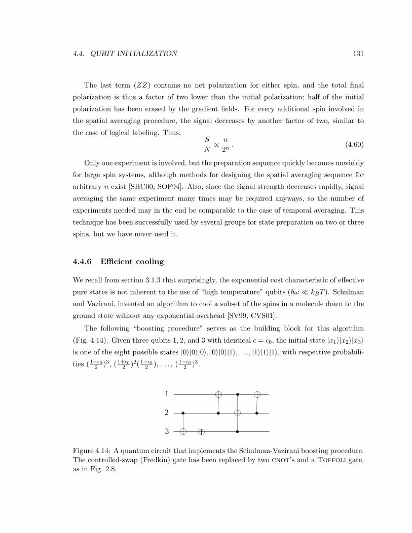
4.4. QUBIT INITIALIZATION 131
The last term (ZZ) contains no net polarization for either spin, and the total final
polarization is thus a factor of two lower than the initial polarization; half of the initial
polarization has been erased by the gradient fields. For every additional spin involved in
the spatial averaging procedure, the signal decreases by another factor of two, similar to
the case of logical labeling. Thus,S
N∝ n
2n. (4.60)
Only one experiment is involved, but the preparation sequence quickly becomes unwieldy
for large spin systems, although methods for designing the spatial averaging sequence for
arbitrary n exist [SHC00, SOF94]. Also, since the signal strength decreases rapidly, signal
averaging the same experiment many times may be required anyways, so the number of
experiments needed may in the end be comparable to the case of temporal averaging. This
technique has been successfully used by several groups for state preparation on two or three
spins, but we have never used it.
4.4.6 Efficient cooling
We recall from section 3.1.3 that surprisingly, the exponential cost characteristic of effective
pure states is not inherent to the use of “high temperature” qubits (~ω kBT ). Schulman
and Vazirani, invented an algorithm to cool a subset of the spins in a molecule down to the
ground state without any exponential overhead [SV99, CVS01].
The following “boosting procedure” serves as the building block for this algorithm
(Fig. 4.14). Given three qubits 1, 2, and 3 with identical ε = ε0, the initial state |x1〉|x2〉|x3〉is one of the eight possible states |0〉|0〉|0〉, |0〉|0〉|1〉, . . . , |1〉|1〉|1〉, with respective probabili-
ties (1+ε02 )3, (1+ε0
2 )2(1−ε02 ), . . . , (1−ε0
2 )3.
1
2
3
Figure 4.14: A quantum circuit that implements the Schulman-Vazirani boosting procedure.The controlled-swap (Fredkin) gate has been replaced by two cnot’s and a Toffoli gate,as in Fig. 2.8.

132 CHAPTER 4. LIQUID-STATE NMR QUANTUM COMPUTING
First perform a cnot operation on 3 conditioned on the state of 2. The new state of the
three qubits is |x′1〉|x′2〉|x′3〉 = |x1〉|x2〉|x2 ⊕ x3〉, where ⊕ denotes addition modulo 2. Note
that conditioned on |x′3〉 = |0〉, the polarization of 2 is now 2ε01+ε02 (2 is almost twice as “cold”
as before); conditioned on |x′3〉 = |1〉, the polarization of 2 is 0 (2 is at infinite temperature).
However, overall, the polarization of 2 is still the same as before, ε0. The polarization of 1
is of course also still ε0. We then perform a not operation on 3 followed by a Fredkin gate
with 3 as the control qubit. The result is that 1 and 2 are swapped if and only if |x′3〉 = |0〉(and thus if and only if 2 has been cooled): |x′′1〉|x′′2〉|x′′3〉 = |x′2〉|x′1〉|x′3〉 if |x′3〉 = |0〉, and
|x′′1〉|x′′2〉|x′′3〉 = |x′1〉|x′2〉|x′3〉 otherwise. On average, 1 will thus be colder than before. The
resulting polarization of 1 is ε = 3ε02 +O(ε), where the higher order terms are negligible,
so the polarization of spin 1 is enhanced by a factor of 3/2.
In order to achieve increasingly higher polarizations, this boosting procedure must be
applied repeatedly, whereby a fraction of the cold spins obtained from one round is made
progressively colder in the next. Spins of little or no polarization are discarded in each
round. Analyzing the polarization transfer using energy and temperature considerations,
Schulman and Vazirani showed [SV99] that the progression of rounds can be arranged so
that k bits with nearly optimal enhancement can be extracted, approaching the entropy
bound of Eq. 3.7. Furthermore, the number of elementary operations (pulses and delay
times in NMR) required to accomplish the entire process is only O(n logn). In summary,
the highly random initial state of room temperature nuclear spins represents no funda-
mental obstacle to scalable quantum computation.
However, the prefactor in the overhead in the number of spins is n/k ≈ 1/ε20 (Eq. 3.10,
for small ε0), which is unreasonably high (about 109) for thermally equilibrated nuclear
spins at room temperature with current magnetic field strengths. It means we would need
a molecule with at least k109 spins in order to obtain a k-qubit computer. This is clearly
impractical.
Until hyperpolarization techniques become much more advanced, the significance of the
Schulman-Vazirani scheme for NMR quantum computing is thus purely at a fundamental
level: NMR quantum computing is in principle scalable. However, for systems with much
higher initial polarizations, Schulman-Vazirani cooling can be very useful if it is difficult to
otherwise obtain completely pure qubits.
4.5. READ-OUT 133
4.5 Read-out
4.5.1 NMR spectra
Measurement procedure
The magnetic signal of a single nuclear spin is to weak to be directly detected9. Therefore,
NMR experiments are done using a large ensemble of identical molecules, typically on the
order of 1018, disolved in a liquid solvent. The same10 operations are applied to all the
molecules in the ensemble, so the final state of the spins is the same in all molecules.
The measurement is done with an RF coil mounted next to the sample (section 5.1),
which records the oscillating magnetic signal produced by the transverse component of the
magnetic moment of the precessing spins (the longitudinal component does not precess and
is not picked up by the coil); this time-domain signal is Fourier-transformed in order to
obtain a spectrum.
Different spins (qubits) in a molecule are spectrally distinguishable via their Larmor
frequencies ωi (section 4.1), and the amplitude and phase of the different spectral lines give
information about the respective spin states. Mathematically, the time-domain signal of
spin i can be expressed as
V (t) = 2V0Tr[e−iHt/~ρ(0)eiHt/~(−iIix − Iiy)
], (4.61)
where ρ(0) is the density matrix at the start of the measurement and V0 is the maximum
signal strength (discussed on page 136). The phases of the observable (−iIix − Iiy) are
chosen11 such that a positive absorptive line corresponds to a spin along −y, a negative
absorptive line to a spin along +y, and positive and negative dispersive lines to a spin along
+x and −x respectively. Eq. 4.61 represents the signal in the lab frame, but by mixing the
signal with a reference oscillator at ωi0, we obtain instead the expectation value of −iIix− Iiyin the rotating frame, which is the relevant reference frame for quantum computing. If ρ
is mixed, as is the case in room temperature experiments, the expectation value represents
an averaged read out over the statistical mixture of states. What we observe is the excess
9Under certain circumstances, the spin states can be inferred via optical techniques. This is the case forexample in ion traps.
10This requires extremely homogeneous magnetic fields (both DC and RF). In practice, the operationsapplied to different molecules are only approximately the same (see section 5.1).
11Other authors have adopted different conventions.

134 CHAPTER 4. LIQUID-STATE NMR QUANTUM COMPUTING
of spins in the most populated state(s).
Since a spin along the ±z axis of the Bloch-sphere, which corresponds to the |0〉, |1〉basis, does not produce an NMR signal, we have to change basis via a Rx(90) read-out
pulse in order to perform a measurement in the |0〉, |1〉 basis. With the above phase
conventions, a spin in |0〉 before the read-out pulse will give a positive absorptive line after
the read-out pulse, and a spin in |1〉 will give a negative line. Inspection of the spectrum
acquired after a read-out pulse thus immediately reveals the projection of the spin state
onto the |0〉, |1〉 basis just before the read-out pulse.
Measurement process
What is really happening to the spins during the measurement process? What difference
does it make whether or not an observer looks at the signal, or even whether the signal
is recorded? And why can we accurately measure both the (non-commuting) x and y
components of the state of a quantum mechanical object ?
The measurement of the spin states in NMR is a weak measurement (see section 3.1.4):
the measuring apparatus, the RF coil, is present all the time, but it is only very weakly
coupled to the nuclear spins and contributes very little to decoherence. Of course, the spins
still decohere through interactions with other spins and with the “bath”, and in addition the
spins dephase due to ~B0 inhomogeneities. The oscillation of the magnetic signal therefore
decays over time (usually exponentially). The decaying time domain signal pick up the the
RF coil is called the free induction decay (FID).
If the envelope of the FID decays as e−t/T (usually T = T ∗2 , defined in section 4.6), the
Fourier transform of the FID is a Lorentzian line,
∝ 11 + (ω − ω0)2
− iω
1 + (ω − ω0)2, (4.62)
which has a linewidth at half height of
∆f =∆ω2π
=1
2πT. (4.63)
Since the measurement is weak, only very little information can be obtained about the
state of individual spins. However, thanks to the large number of identical molecules in an
NMR sample, we can acquire much more information about the (average) spin state than

4.5. READ-OUT 135
we could even in principle ever obtain about the state of an individual spin. For example,
the built-in averaging nature of ensemble measurements allows us to directly measure the
expectation value of two non-commuting observables.
Ensemble averaged measurements can thus in some respects provide more information
than projective measurements on single quantum systems. At the same time, averaging
erases certain information which quantum algorithms rely on. Fortunately, all current quan-
tum algorithms can be modified to circumvent this difficulty, as explained in section 3.1.4.
Multiplet fine structure
Extra information about the spin states is contained in the multiplet fine structure of the
spectra. The spectrum of each spin in a n-spin molecule may be split in up to 2n−1 lines,
due to J-coupling terms in the Hamiltonian which modulate the time domain signal of
Eq. 4.61 by J Hertz. After we have determined the magnitude and sign of the J couplings,
we can then associate each line in the multiplet with the state of the other spins, as shown
in Fig. 4.15 for a five-spin molecule.
−50 0 500
2
4
6
8
10
0000
0010
0001
0011
0100
0110
0101
0111
1111
1101
1110
1100
1011
1001
1010
1000
Figure 4.15: The thermal equilibrium spectrum (amplitude of the real part) of spin 1in a molecule of five coupled spins (more details on this molecule are given in section 5.9).Frequencies are given in units of Hz, with respect to ω1
0. The state of the remaining spins is asindicated, based on J12 < 0 and J13, J14, J15 > 0; furthermore, |J12| > |J13| > |J15| > |J14|.
The presence or abscence of specific lines in a multiplet of one spin can thus reveal
information about the other spins. For example, for an effective pure ground state (sec-
tion 4.4.2), the only line we expect to see in the spectrum of Fig. 4.15 is the line labeled
0000. Similarly, in logical labeling (section 4.4.3), the multiplet structure can be used to

136 CHAPTER 4. LIQUID-STATE NMR QUANTUM COMPUTING
identify the logically labeled subspace. We have used the extra information in the fine
structure in many of the experiments presented in chapter 5.
Signal-to-noise ratio
The maximum NMR signal, V0, measured via a pick-up coil after applying a read-out pulse
to a spin in thermal equilibrium, is proportional to
1. the number of molecules, which is linear in the volume, V , and the concentration, nc,
2. the number of equivalent sites, ne, in the molecule for the spin (e.g. this number is
three for 1H in CH3Cl),
3. the equilibrium polarization, ε0, which is proportional to γ, B0 and 1/Ts, where Ts is
the absolute temperature of the sample,
4. ω0 (because the measurement is inductive), which is proportional to γ and B0,
5. the quality factor, Q, of the coil,
6. the filling factor, η, (the fraction of the coil volume occupied by the sample),
7. a factor, K, which depends on the coil geometry and reflects the coupling of the spins
to the coil.
The noise in NMR measurements is normally dominated by the thermal noise of the
coil. The rms noise amplitude is proportional to the square root of
1. the absolute temperature of the coil, Tc,
2. the shunt resistance of the tuned circuit, R = QLω0, (L is the inductance),
3. the width of the narrow band audio-filter, ∆f .
How much the lines in an NMR spectrum rise above the noise level depends not only on
the actual signal strength and noise level, but also on the degree to which the signal is spread
out in frequency. Thus, the signal-to-noise ratio of an NMR spectrum is also proportional
to 1/m, where m is the multiplicity of the multiplet, and to T ∗2 , as∫∞
0 exp(−t/T ∗2 ) = T ∗2 (a
long T ∗2 gives narrow and thus tall lines).

4.5. READ-OUT 137
In summary, the signal-to-noise ratio can be expressed as
S
N∝ ncV neγ
2B20QηKT
∗2
mTs(TcQLγB0∆f)1/2=ncV neγ
3/2B3/20 Q1/2ηKT ∗2
mTs(TcL∆f)1/2. (4.64)
In practice, many of these parameters are interdependent. For a more detailed discussion
of the signal-to-noise ratio, see Ref [HR76].
4.5.2 Quantum state tomography
The spectra of a few select spins suffice to obtain the answer to a computation. Nevertheless,
the full density matrix conveys a lot of extra information, which can be used to expose the
presence of errors not visible in the single output spectra and furthermore is a useful tool
for debugging pulse sequences.
The procedure for reconstructing the density matrix is called quantum state tomogra-
phy [CGKL98, CGK98, CVZ+98]. In order to explain the idea behind this procedure, we
take another look at the signal of Eq. 4.61. The operator −iIix − Iiy selects specific entries
in the density matrix, called single quantum coherence (SQC) elements. The SQC elements
“connect” basis states which differ by only one quantum of energy (for example |00〉 ↔ |01〉but not |00〉 ↔ |11〉). The SQC elements of a two-spin density matrix are
. . × .
. . . ×× . . .
. × . .
and
. × . .
× . . .
. . . ×
. . × .
(4.65)
for spins 1 and 2 respectively. We recall that the density matrix is Hermitian, so the entries
above and below the diagonal (going from upper left to lower right) are each other’s complex
conjugate. In Eq. 4.65, there are thus only two independent SQC elements for each spin.
Those complex numbers are directly proportional to the area underneath the two spectral
lines in each of the doublets of the two-spin spectrum. For an n spin system, the 2n−1 lines
within each multiplet can be identified with 2n−1 SQC elements per spin.
Quantum state tomography then consists of repeating the computation many times,
each time looking at the final state of the spins “from a different angle”, by applying
different sets of read-out pulses which rotate different elements of the density matrix into
observable positions. In an idealized experiment (no imperfections), the density matrix
138 CHAPTER 4. LIQUID-STATE NMR QUANTUM COMPUTING
uniquely follows from the area underneath the individual lines within all the multiplets. In
real experiments, all the spectral information may not be compatible with each other, but
we can obtain a good estimate of the actual density matrix via a least-squares fit.
Since quantum state tomography involves on the order of 4n experiments (the number
of degrees of freedom in the density matrix), it is practical only for experiments involving
a few spins; we have reconstructed density matrices only for experiments with two or three
spins (sections 5.3- 5.7).
4.6 Decoherence
The decoherence process of uncoupled nuclear spins is well described by a combination of
two phenomena: longitudinal and transverse relaxation12 [Abr61, Sli96]. These two pro-
cesses are closely related to generalized amplitude damping and phase damping respectively,
which have been described mathematically in section 3.1.5. We will first present the main
decoherence mechanisms and then describe standard methods to measure the characteristic
relaxation time constants.
4.6.1 Principal mechanisms
Relaxation of nuclear spins is caused by fluctuations in the magnetic field experienced by the
spins. Whether the magnetic field fluctuations contribute to energy exchange with the bath
or phase randomization depends on the time scale of the fluctuations. Roughly speaking,
we have that
• fluctuations at ω0 lead to efficient energy exchange with the spins (the bath and the
spins act as RF transmitters and receivers tuned to the same frequency),
• fluctuations at zero frequency, i.e. slow fluctuations, give rise to phase randomization.
Depending on the mechanism, however, fluctuations at ω0 and at 2ω0, may also con-
tribute to phase randomization. Similarly, fluctuations at 2ω0 may also contribute to energy
exchange. Finally, if two or more coupled spins are present, energy exchange is also pro-
moted by fluctuations at the sum and difference frequencies of the spins (ωi0 ± ωj0) [Abr61].
12For coupled spins (dipole coupled or J coupled), the decoherence process also includes cross-relaxationand the nuclear Overhauser effect (NOE), but we shall not discuss those here.
4.6. DECOHERENCE 139
The following mechanisms at a microscopic scale contribute to relaxation of nuclear
spins in liquid solution:
1. Intermolecular dipole-dipole interactions with nuclear spins.
This interaction is modulated by molecular translation and rotation and contributes
to phase randomization (T2). It can be dominant in relatively large molecules, when
all the high-γ nuclei are well separated in the molecule.
2. Intramolecular dipole-dipole interactions with nuclear spins.
This interaction fluctuates due to molecular tumbling; its contribution to T1 scales as
T−11 ∝ γiγj/rij , where γi and γj are the gyromagnetic ratios for spins i and j, and rij
is the distance between the two nuclei.
3. Intra- and intermolecular dipole-dipole interactions with electron spins.
If unpaired electrons are present, such as in paramagnetic ions and free radicals, this
decoherence mechanism will usually dominate because electrons have a much large
magnetic moment than the nuclei.
4. Chemical shift anisotropy.
If the chemical shift is anisotropic, it rapidly fluctuates due to molecular tumbling.
This effect increases with magnetic field strength as T−11 ∝ B2
0 (chemical shifts are
linear in the field strength).
5. Spin-rotation interaction.
Molecular rotations create magnetic fields which are modulated due to collisions. This
mechanism is important especially in small, symmetric molecules.
6. Scalar coupling.
Rapid fluctuations in the J coupling contribute to relaxation.
7. Quadrupolar coupling.
Nuclei with a spin quantum number larger than 1/2 don’t have a spherically sym-
metric nuclear charge. As a result, such nuclei interact with electric field gradients.
Fluctuations in the electric field gradient due to molecular tumbling cause quadrupolar
nuclei to relax very fast.

140 CHAPTER 4. LIQUID-STATE NMR QUANTUM COMPUTING
8. Coupling to quadrupolar nuclei.
The rapidly fluctuating spin state of quadrupolar nuclei contributes to relaxation of
other spins.
9. Chemical exchange.
Fast chemical exchange of part of a molecule causes the chemical shifts of nuclei in
the remaining part of the molecule to rapidly jump back and forth between two or
more values.
In addition, fluctuations due to noisy RF amplifiers or other external sources which emit
electro-magnetic fields at ω0 shorten T1. Similarly, magnetic field inhomogeneities (in B0
or B1) shorten the apparent T2. However, magnetic field inhomogeneities can in principle
be easily unwound via refocusing pulses, provided diffusion rates are slow compared to the
time scale of the operations. The literature therefore distinguishes between T2, the intrinsic
transverse relaxation time constant, and T ∗2 , which incorporates both intrinsic relaxation
and inhomogeneous broadening.
Minimizing relaxation
To some degree, relaxation is influenced by parameters under the control of the experi-
menter. For quantum computation, it is crucial to maximally take advantage of the possi-
bilities to reduce relaxation.
A first set of guidelines hinges on the idea of motional narrowing. Rapid molecular
tumbling shortens the correlation times of many fluctuations and therefore tends to lengthen
T2 (which is usually much shorter than T1). The tumbling rate depends on the following
parameters:
1. Molecule size: small molecules tumble more easily.
2. Viscosity of the solvent: lower viscosity obviously promotes rapid tumbling (super-
critical solvents are ideal from this point of view, as they combine the high density
and solubility of liquids with the low viscosity of gases).
3. Temperature: higher temperatures provide more thermal energy for tumbling and also
tend to reduce solvent viscosity.
Additional guidelines for sample preparation and molecule selection are:

4.6. DECOHERENCE 141
1. Remove oxygen and other paramagnetic impurities from the solution.
2. Avoid quadrupolar nuclei in the molecule.
3. Reduce the solute concentration in order to reduce intermolecular relaxation, and
choose solvents preferrably with nonmagnetic nuclei or low-γ nuclei, or else with
different nuclear species than those in the solute molecule, because like nuclei relax
each other more efficiently than unlike nuclei.
4. Remove reagents with which the molecule may exchange chemically.
Finally, non-intrinsic relaxation can be minimized by
1. making the B0 field as homogeneous as possible.
2. Spinning the sample about the z axis in order to average out the remaining transverse
field inhomogeneities.
3. Filter out particles in the solvent, as they create magnetic field inhomogeneities (as-
suming their magnitic susceptibility is different than that of the solvent).
4. Using RF coils with good homogeneity.
5. Blanking the amplifiers in between RF pulses.
6. Reduce radiation damping by reducing the sample concentration or lowering the Q
of the probe (during a pulse, the spins are tipped into the transverse plane, so they
induce a voltage in the coil which in turn tips the spins back).
4.6.2 Characterization
We have used the following (standard) procedures for measuring the T1, T2 and T ∗2 [Fre97].
Inversion recovery constitutes a clean measurement of T1. First, a 180 pulse inverts
the spin from +z to −z; then the spin is allowed to relax back to its equilibrium state +z
for a variable duration t; finally, a 90 read out pulse tips the spin into the xy plane and
the signal is recorded. The pulse sequence is thus
X2 − t−X − acquisition . (4.66)

142 CHAPTER 4. LIQUID-STATE NMR QUANTUM COMPUTING
With properly set receiver phase settings, the peak height of the measured spectrum varies
with t as
S = S0
[1− αe−t/T1
], (4.67)
where α is a fitting parameter which compensates for incomplete inversion due to RF field
inhomogeneities (ideally α = 2). Typical values for T1 are a few seconds to a few tens of
seconds.
T ∗2 is the time constant of the free induction decay, so T = T ∗2 in Eq. 4.63 (assuming the
line is Lorentzian, which is not necessarily the case in an inhomogeneous magnetic field),
and
∆f =∆ω2π
=1
2πT ∗2. (4.68)
We can thus easily derive T ∗2 from the linewidth at half height. Measurement of T2 requires
that dephasing due to magnetic field inhomogeneities be refocused. The standard measure-
ment for T2 is the Carr-Purcell-Meiboom-Gill (CPMG) pulse sequence. First a Y pulse
takes the spin to +x. Then, the subsequence
τ
4X2 τ
2X2 τ
4(4.69)
is repeated k times, where k is arrayed, and the signal is recorded for each value of k. Typical
values of τ are 1-10 ms, short enough such that minimal diffusion takes place during the
delay times, and long enough such that the duty cycle (the ratio of the duration of the
pulses over the delay times) is not too high. The measured signal will decay exponentially
with the total decay time t = kτ ,
S = S0 e−t/T2 . (4.70)
In theory for small molecules T2 ≈ T1, although in practice T2 values were a few tenths of
a second to a few seconds in the molecules we have used, substantially shorter than T1.
We note that the measured values of T2 (and T ∗2 ) do not correspond exactly to the
phase damping time constants defined in section 3.1.5. The CPMG measurement gives the
decay rate of the single quantum coherence elements of the density matrix, to which both
amplitude damping and phase damping contribute. However, in practice, often T1 T2 in
which case the CPMG measurement does give the phase damping time constant, to good
approximation.
4.7. MOLECULE DESIGN 143
Finally, the T2 measurement is affected by coupled evolution, in particular when τ is
on the order of 1/2J . In a multi-spin system, it becomes difficult to choose τ so it is
different enough from 1/2J for the various J-coupling strengths. Different choices of τ give
considerably different measured T2’s, so their meaning is diminished [VV78].
4.7 Molecule design
The choice of a suitable molecule is crucial for the success of NMR quantum computing
experiments. The fundamental properties which make a molecule suitable for quantum
computation follow from the preceding sections.
First, the number of spin-1/2 nuclei in the molecule must be equal or larger than the
required number of qubits. Reasonable choices for qubits include 1H, 13C, 15N, 19F and 31P,
as they all have a spin-1/2 nucleus, and are found relatively easily in small organic molecules
(however, isotopic labeling is needed to obtain 13C and 15N in high concentration).
Second, in order to be able to complete a large number of two-qubit operations within
the coherence time, we desire
|Jij | 1T2,
1T1. (4.71)
Third, in order to have sufficiently slow coupled evolution during spin-selective shaped
pulses, we need |ω1| |Jij | and since spin-selectivity requires |ωi0 − ωj0| > |ω1|, we desire
|ωi0 − ωj0| |Jij | . (4.72)
This condition at the same time ensures that the spectra are first order. We note that
Eqs. 4.71 and 4.72 automatically guarantuee that |ωi0 − ωj0| 1/T2, 1/T1, such that many
one-qubit operations can be done within the coherence time as well.
Eq. 4.72 is exceedingly well satisfied in heteronuclear molecules. In homonuclear molecules,
strong chemical shifts are promoted by strong asymmetries in the molecule. The normal
range of chemical shifts is about 200 ppm for 19F (about 100 kHz at 10 Tesla), 200 ppm for13C nuclei (about 25 kHz), 10 ppm for 1H (about 5 kHz) and > 300 ppm for 15N (about 7.5
kHz). In homonuclear molecules, 19F and 13C are thus preferred. 19F and 13C also tend to
have strong J couplings, needed to satisfy Eq. 4.71 while 1H often has smaller J couplings.
On the one hand, low-γ nuclei such as 15N and 13C tend to have longer coherence times
than high-γ nuclei such as 1H and 19F. On the other hand, high-γ nuclei such as 1H and

144 CHAPTER 4. LIQUID-STATE NMR QUANTUM COMPUTING
19F have the advantage that they give the strongest signals (recall Eq. 4.64). 13C, 15N have
a low γ, and the γ of 31P is intermediate (see Table 4.1).
Section 4.6.1 discusses several other elements related to molecule design which affect the
coherence time.
We have already seen (section 4.3) that Eq. 4.71 is not binding. This condition can be
extended to say that a sufficient network of J ’s larger than 1/T2 must be available , such
that a two-qubit gate between any pair of spins (implemented directly or indirectly) takes
a short time compared to the coherence time.
Similarly, Eq. 4.72 assumes that we need to individually address all the spins, but this
isn’t always necessary either (section 3.1.2). A polymer with a unit cell ABC which repeats
itself n times and terminates on a D (where A,B,C and D have distinct chemical shifts)
can possibly serve as an n qubit computer (Fig. 3.1. The caveat is that it isn’t known how
to set up a proper initial state when using nuclear spins at room temperature in such an
architecture.
Finally, there are several more mundane but even more important practical requirements
for quantum computer molecules: they must be stable (i.e. not decompose) for a reasonably
long time, disolve in an NMR solvent (chloroform, acetone, ether, DMSO, benzene, toluene,
among others), be available or possible to synthesize, be affordable (99% 13C or 15N enriched
compounds can be very expensive) and safe. Indeed, many molecules which one could draw
on the board for their beautiful presumed NMR properties turn out to be unstable, very
hard to synthesize, or toxic.
4.8 Pulse sequence design
A computation with nuclear spins consists of a carefully designed sequence of RF pulses
separated by delay times, corresponding to computational steps. Those elementary instruc-
tions, pulses and delay times, can be viewed as the machine language of an NMR quantum
computer.
The goal of pulse sequence design is to translate a high-level description of a quantum
algorithm into unitary transformations acting on one or several qubits, then to decompose
each unitary operation into one- and two-qubit gates, and finally into pulses and delay
times. This process is analogous to compiling code on traditional computers.
We know from previous sections on quantum gates (2.2) and their implementation in
4.8. PULSE SEQUENCE DESIGN 145
NMR (4.2-4.3) that many pulse sequences result in exactly the same unitary transformation.
Good pulse sequence design therefore attempts to find the shortest and most robust pulse
sequence that implements the desired transformations.
A key point in pulse sequence design is that the process must itself be efficient. For
example, suppose an algorithm acts on five qubits with initial state |00000〉 and that the final
state is (|01000〉+ |01100〉/√
2. The overall result of the sequence of unitary transformations
is thus that qubit 2 is flipped and that qubit 3 is placed in an equal superposition of |0〉and |1〉. This net transformation can obviously be obtained immediately by the sequence
X22Y3. However, the effort needed to compute this net transformation generally increases
exponentially with the problem size, so such extreme simplifications are not practical.
4.8.1 Simplification at three levels
At the most abstract level of pulse sequence simplification, careful study of a quantum
algorithm can give insight in how to reduce the resources needed. For example, we recall
that a key step in both the Deutsch-Jozsa algorithm and the Grover algorithm can be
described as the transformation |x〉|y〉 → |x〉|x⊕ y〉 (see Eqs. 2.64 and 2.70), where |y〉 is set
to (|0〉−|1〉)/√
2, so that the transformation in effect is |x〉(|0〉−|1〉)/√
2→ (−1)f(x)|x〉(|0〉−|1〉)/
√2. We might thus as well leave the last qubit out as it is never changed.
At the next level, that of quantum circuits, we can use the simplification rules such
as those illustrated in Fig. 4.16. In this process, we can fully take advantage of commu-
tation rules to move building blocks around, as illustrated in Fig. 4.17 (see also page 33).
Commutation rules can also tell us which gates can in principle be executed simultaneously.
Furthermore, we can use the fact that U acting on a diagonal density matrix doesn’t need to
have the right phases (e.g. compare Eq. 4.19 and Eq. 4.20). Finally, we can take advantage
of the fact the most building blocks have many equivalent implementations, as shown in
Fig. 4.18.
At the lowest level, that of pulses and delay times, further simplification is possible by
taking out adjacent pulses which cancel out, such as X and X. In fact, we can go one step
further and choose those pulses sequence for each building block which will give the most
cancellation of pulses. For this purpose, it is convenient to have a library of equivalent
implementations for the most commonly used quantum gates. For example, two equivalent

146 CHAPTER 4. LIQUID-STATE NMR QUANTUM COMPUTING
U U
U
0 1
U U
U U
Figure 4.16: Simplification rules for quantum circuits
U U U U UU
Figure 4.17: Commutation of unitary operators can help simplify quantum circuits bymoving building blocks around such that cancellations of operations as in Fig. 4.16 becomepossible. For example, the three components (separated by dashed lines) in these twoequivalent realizations of the Toffoli gate commute with each other and can thus beexecuted in any order.
decompositions of a cnot12 gate (with J12 > 0) are
Z1 Z2X2 1/2J Y2 , (4.73)
where time goes from right to left, and
Z1 Z2 X2 1/2J Y2 , (4.74)
and two equivalent implementations of the hadmard gate on qubit 2 are
X22 Y2 (4.75)
and
Y2X2 . (4.76)
Then, if we want to perform a hadamard operation on qubit 2 followed by a cnot12 gate,
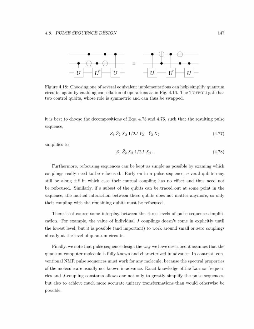
4.8. PULSE SEQUENCE DESIGN 147
UU UU U U
Figure 4.18: Choosing one of several equivalent implementations can help simplify quantumcircuits, again by enabling cancellation of operations as in Fig. 4.16. The Toffoli gate hastwo control qubits, whose role is symmetric and can thus be swapped.
it is best to choose the decompositions of Eqs. 4.73 and 4.76, such that the resulting pulse
sequence,
Z1 Z2X2 1/2J Y2 Y2X2 (4.77)
simplifies to
Z1 Z2X2 1/2J X2 . (4.78)
Furthermore, refocusing sequences can be kept as simple as possible by examing which
couplings really need to be refocused. Early on in a pulse sequence, several qubits may
still be along ±z in which case their mutual coupling has no effect and thus need not
be refocused. Similarly, if a subset of the qubits can be traced out at some point in the
sequence, the mutual interaction between these qubits does not matter anymore, so only
their coupling with the remaining qubits must be refocused.
There is of course some interplay between the three levels of pulse sequence simplifi-
cation. For example, the value of individual J couplings doesn’t come in explicitly until
the lowest level, but it is possible (and important) to work around small or zero couplings
already at the level of quantum circuits.
Finally, we note that pulse sequence design the way we have described it assumes that the
quantum computer molecule is fully known and characterized in advance. In contrast, con-
ventional NMR pulse sequences must work for any molecule, because the spectral properties
of the molecule are usually not known in advance. Exact knowledge of the Larmor frequen-
cies and J-coupling constants allows one not only to greatly simplify the pulse sequences,
but also to achieve much more accurate unitary transformations than would otherwise be
possible.
148 CHAPTER 4. LIQUID-STATE NMR QUANTUM COMPUTING
4.8.2 Design for robustness
The exact choice of pulse sequence greatly affects the robustness against erroneous unitary
evolutions, in particular those due to coupled evolution during pulses and the inhomogeneity
of the RF field used to pulse the spins. In addition to keeping pulse sequences short,
robustness is thus an important consideration in the process of designing pulse sequences.
Undesired coupled evolution can be minimized by choosing suitable pulse shapes (sec-
tion 4.2.4) but also through pulse sequence design, at the lowest level. Simultaneous pulses,
especially 90 pulses, on spins with a large mutual J coupling should be avoided (sec-
tion 4.2.5) and coupled evolution during pulses can be unwound by adjusting the adjacent
refocusing sequences (section 4.2.5).
Erroneous evolution because of RF field inhomogeneity can be very substantial (sec-
tion 5.1), but can in principle be unwound: a X2 pulse causes some spread in the spin
states and we expect a subsequent X2 pulse to unwind this spread quite well, definitely
much better than another X2 pulse. For longer trains of 180 pulses, it isn’t always so easy
to predict which choice of phase for the pulses is most robust to RF field inhomogeneities.
For example, contrary to our intuition, X2X2X2X2 performs much better than X2X2X2X2
and similar extensions exist for longer trains of 180 pulses [LFF82].
Quantum computing pulse sequence are hardly ever so transparant, unfortunately. Ac-
tual refocusing sequences are complicated by the fact that spin-selective 180 pulses on
different spins are interspersed with each other. Furthermore, 90 pulses disturb possible
cancellation between preceding and subsequent 180 pulses.
A general framework for undoing systematic errors such as those due to RF field inhomo-
geneities is highly desirable. This is clearly an ambitious undertaking, but it is encouraging
to know that very strong cancellation of such errors has been observed, even in complex
quantum computing sequences (see sections 5.5 and 5.7).
4.9 Summary
The main message of this chapter is that nuclear spins in molecules in liquid solution largely
satisfy the five requirements for the implementation of quantum computers:
1.√
spin-1/2 nuclei in a molecule are well-defined qubits,
4.9. SUMMARY 149
2.√
the dynamics of coupled nuclear spins can be controlled via RF pulses and delay
times, even though certain terms in the Hamiltonian cannot be switched off,
3. (√
) room temperature nuclear spins can be made to look like they are at zero tem-
perature, although currently only at an exponential cost,
4.√
the state of each qubit can be read out spectroscopically, provided a large ensemble
of molecules is used,
5.√
nuclear spins have long coherence times (easily a few seconds).
In the next chapter, we will present a series of experiments in which we explore how these
methods and concepts translate into the reality of actual quantum computations.

Chapter 5
Experimental realization of NMR
quantum computers
After a description of the experimental apparatus1, we will give a brief overview of the
experimental NMR quantum computing work performed to date (section 5.2). We then
present in detail a series of eight experiments in which we explored quantum computing in
practice. These are an early quantum computation (5.3), an early quantum error detec-
tion experiment (5.4), an explicit demonstration of cold dynamics using room temperature
spins (5.5), a quantum computation performed in a liquid crystal solvent (5.6), a study of
systematic errors with three spins (5.7), an implementation of efficient cooling of one out
of three spins (5.8), a realization of the order-finding algorithm with five qubits (5.9) and
prime factorization of the number fifteen using seven spins and Shor’s algorithm (5.10).
5.1 Experimental apparatus
Figure 5.1 schematically shows the main components of an NMR spectrometer. A sample
containing a large number of identical molecules disolved in liquid solution is placed in
a strong magnetic field. Radio-frequency pulses are applied to the sample via a radio-
frequency coil and the same coil is used to detect the magnetic signal of the spins during
read out. The whole experiment is controlled by a workstation. We now describe each
1The experiments of sections 5.3 and 5.4 took place in the Chemistry Department at Stanford University.The remaining experiments took place at the IBM Almaden Research Center. Both NMR spectrometers arelargely identical, but where they differ, the description is for the instrument at IBM.
150

5.1. EXPERIMENTAL APPARATUS 151
component in more detail.
B0
RF coil
static field coil
sample tube
computeroscillator
RFtransmit/receive
power
preamplifier
switch
amplifier
Figure 5.1: Schematic overview of an NMR apparatus.
5.1.1 Sample
The heart of an NMR quantum computer is a molecule containing several atoms with
spin-1/2 nuclei. In practice, the signal from a single molecule is too weak to be detected
with current techniques, so on the order of 1018 molecules are used in order to boost the
signal. Each molecule in the ensemble acts as an individual quantum computer, and all
1018 quantum computers go through the same operations. The fact that there are many
molecules in the sample does not increase the power of the computer; it just increases the
signal strength. The power of the computer depends only the number of spins per molecule
(see section 4.7 for a discussion of molecule design).
The molecules are disolved in a liquid solvent at room temperature and atmospheric
pressure. Solvent selection is based on the solubility of the quantum computer molecule in
the solvent and on the coherence time of the qubits obtained in the solvent, which depends
on residual couplings between spins in the solvent and in the solute (see section 4.6). The
solute concentration is a trade-off between signal strength and coherence times.
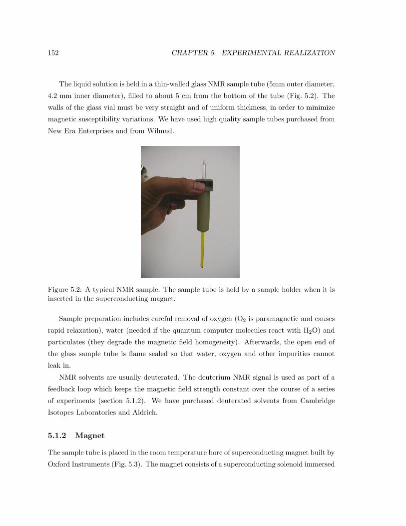
152 CHAPTER 5. EXPERIMENTAL REALIZATION
The liquid solution is held in a thin-walled glass NMR sample tube (5mm outer diameter,
4.2 mm inner diameter), filled to about 5 cm from the bottom of the tube (Fig. 5.2). The
walls of the glass vial must be very straight and of uniform thickness, in order to minimize
magnetic susceptibility variations. We have used high quality sample tubes purchased from
New Era Enterprises and from Wilmad.
Figure 5.2: A typical NMR sample. The sample tube is held by a sample holder when it isinserted in the superconducting magnet.
Sample preparation includes careful removal of oxygen (O2 is paramagnetic and causes
rapid relaxation), water (needed if the quantum computer molecules react with H2O) and
particulates (they degrade the magnetic field homogeneity). Afterwards, the open end of
the glass sample tube is flame sealed so that water, oxygen and other impurities cannot
leak in.
NMR solvents are usually deuterated. The deuterium NMR signal is used as part of a
feedback loop which keeps the magnetic field strength constant over the course of a series
of experiments (section 5.1.2). We have purchased deuterated solvents from Cambridge
Isotopes Laboratories and Aldrich.
5.1.2 Magnet
The sample tube is placed in the room temperature bore of superconducting magnet built by
Oxford Instruments (Fig. 5.3). The magnet consists of a superconducting solenoid immersed

5.1. EXPERIMENTAL APPARATUS 153
in a bath of liquid Helium (at 4.2 Kelvin). The Helium vessel is surrounded by a vacuum
seal, a liquid Nitrogen vessel and another vacuum seal. The whole magnet is mounted on
air-cushioned vibration isolation legs.
A persistent current of about 100 A through the windings of the solenoid produces a
magnetic field in the bore of 11.7 Tesla, reasonably strong for an NMR magnet and about
200,000 times the strength of the earth’s magnetic field. The resulting Larmor frequencies
are in the range of 50 to 500 MHz (see Table 4.1). About three meters away from the
center of the magnet, the stray magnetic field is still about five Gauss (10 times the earth’s
magnetic field). Clearly, it is important to keep all magnetic objects away from the magnet,
as they may otherwise be pulled in and damage the magnet.
Figure 5.3: Oxford Instruments 500 MHz wide-bore NMR magnet. Fill ports for liquidnitrogen and helium stick out from the top. The cabinet near one of the magnet legscontains transmit/receive switches, preamplifiers and mixers. The probe is inserted in thebore of the magnet from below and the sample is inserted from the top. It sits in the probein the center of the solenoid.
Strong fields are advantageous because the separation between the spectral lines of
nuclei of the same isotope (the chemical shift) increases linearly with the field strength.
Large frequency separations make it easier to address each qubit individually. However,
spin coherence times may decrease as the field goes up (relaxation due to chemical shift

154 CHAPTER 5. EXPERIMENTAL REALIZATION
anisotropies increases as the field increases), so it isn’t clear that an even stronger field
would be better for quantum computing.
The bore diameter of our magnet is 89 mm, compared to 52 mm for standard magnets
intended for liquid state NMR. The extra space permits the use of custom-built probes
with better performance than the commercially available liquids probes, although we did
use narrow-bore probes in all the experiments presented in this work.
Of crucial importance is the homogeneity of the magnetic field, as it directly affects
the spectral linewidths and thereby both the signal-to-noise ratio and the overlap of lines
within a multiplet. An inhomogeneous field also causes dephasing in the course of a pulse
sequence, although this can in large part be refocused.
Two sets of shimming coils mounted around the bore produce magnetic fields which
even out any inhomogeneities in the field of the main solenoid. One set consists of about
ten superconducting coils, which are energized upon installation and never readjusted. The
current of the second set of about 25 room temperature coils can be adjusted by the user.
Each shimming coil creates a magnetic field with a specific spatial variation in strength: the
field strength of the Z1 coil varies linearly along the z axis, the Z2 coil varies quadratically
along z and so forth. A typical set of shimming coils contains Z coils up to fifth or sixth
order, transverse (X and Y ) coils up to fourth order, and combined coils (e.g. X2Z) up to
fourth order as well.
The optimal shim settings are sensitive to the RF coil geometry, the solvent suscepti-
bility, the sample height, the glass tube dimensions and susceptibility, the temperature and
the presence of magnetic objects in the vicinity of the magnet. The homogeneity of the coil
can be assessed via the lock signal strength (see below), the shape and decay rate of the
FID and the lineshape and linewidth. With a lot of effort, variations in the strength of the
static magnetic field can be made better than 1 part in 2× 10⁹ over the active region of the
sample (4.2 mm in diameter by 1.5 to 2 cm in height), giving linewidths of only 0.2 Hz at
500 MHz 2, a truly extraordinary homogeneity.
A second important consideration is that the field strength of a superconducting magnet
slowly drifts over time, as the current through the windings does dissipate power, albeit
2At this point, the intrinsic T2 of most samples dominates the linewidth. In fact, with most samples it isnot possible to obtain such narrow lines.

5.1. EXPERIMENTAL APPARATUS 155
only a tiny amount. For a good NMR magnet, the drift is below one Hertz per hour. To
put this in perspective, at a drift rate of 1 Hz/hr the field decreases by only 8.76 kHz per
year, which is 8.76 kHz / 500 MHz < 0.002% per year. An NMR magnet can thus easily
be used for several decades without any substantial loss in field strength.
Even though the field drift is very slow, it is still appreciable in experiments where
precise control over the spin dynamics is required, as is the case of quantum computation.
The spin Larmor frequencies slowly drift away from the RF source frequencies so pulses will
be off-resonance. Furthermore, the rotating reference frame provided by the RF sources
gets progressively out of phase with the actual rotating frame of the spins.
The drift of the magnetic field is therefore compensated for via a room temperature Z0
coil which superimposes a magnetic field on top of the field produced by the main solenoid.
The current through the compensating coil is regulated via a feed-back loop aimed at locking
the frequency of the deuterium signal of the solvent (and thus also the field strength) to a
prescribed value; the deuterium nuclei in the solvent are pulsed every few seconds, and the
deuterium signal is monitored (the deuterium frequency is 77 MHz, far away from other
frequencies of interest). At the start of a series of experiments, the user must set up the
lock power and the gain and phase of the lock feed-back signal. From then on, the lock
mechanism operates automatically in the background.
Other possible solutions for B0 drift include making the RF source frequencies track the
drifting Larmor frequencies, or the use of additional 180 pulses to refocus chemical shift
evolution. The latter involves additional pulses and is not desirable.
5.1.3 Probe
The probe is in a cylindrical aluminum housing (Fig. 5.4) which contains the RF coils, a
tuning and matching electrical circuit, a temperature control system, a sample spinning
mechanism and sometimes gradient coils.
RF coils and tune/match circuits
Saddle-shaped Helmholtz RF coils mounted near the top of the probe closely surround the
glass sample tube over a height of about 1.5 cm. The region of the sample which is well
coupled to the coils, called the active region, is a little larger than the region surrounded
by the RF coil, usually about 2cm. The coils typically have only one to three windings,

156 CHAPTER 5. EXPERIMENTAL REALIZATION
and are made of low-resistivity metals such as copper or Pd-plated copper foil or Al filled
copper wire in order to compensate for susceptibility differences.
Figure 5.4: Nalorac HFX Probe. The RF coils sit near the top of the probe. BNC connec-tors, a cooling air inlet, a connector for the gradient coils and knobs to adjust to tune/matchcapacitors are visible at the bottom of the probe.
The coils are incorporated in a resonant circuit tuned to the Larmor frequency of one or
several nuclei, in order to obtain a high quality factor Q (values of 100 to 300 are typical),
and thus a high signal-to-noise ratio (Eq. 4.64). The exact resonance frequency of the circuit
can be adjusted via a mechanically variable capacitor. Using a second variable capacitor,
the impedance of the circuit is matched to 50Ω. The tune and match capacitors are usually
mounted close by the coil, and are adjustable via long mechanical rods which stick out from
the bottom of the probe. Probe tuning and matching is done by minimizing the reflected
power for the desired frequencies.
Because of the difficulty of building high Q resonant circuits with multiple resonances
over a wide frequency range, many commercial probes contain two pairs of Helmholtz coils,
mounted at right angles with little overlap such that there is little cross-talk between the
twe sets of coils. One coil then serves the high-band nuclei 1H and 19F (500 and 470 MHz
at 11.7 T) and the other coil serves the low-band nuclei (the highest of which is 31P, at 202
MHz). The lock (2H, at 77 MHz) is usually on the high-band coil such that the lock signal
interferes as little as possible with the other low-band signals. Our probe is a “normal”
probe, with the high-band coil on the inside; “inverse” probes have the high-band coil on

5.1. EXPERIMENTAL APPARATUS 157
the outside.
The sensitivity of a probe depends not only on the Q but also on the filling factor η
and the geometrical coupling K between the coils and the spins (Eq. 4.64). Because of
the reciprocity between transmitting and receiving RF signals, a convenient measure for
the sensitivity is the minimum 90 pulse length for a given power and coil volume. The
absolute minimum achievable 90 pulse length (typically 6 − 15µs) depends also on how
much power the probe can take before the coil windings or the capacitors arc.
The RF field homogeneity of saddle shaped Helmholtz coils is quite poor: the envelope
of the Rabi oscillation decays by about 5% per 90 rotation. In other words, the error
of a single one-qubit rotation just due to RF coil inhomogeneity is on the order of 5%.
Fortunately, the effects of this error can, at least in principle, be largely undone by clever
pulse sequence design (sections 4.8 and 5.7).
More homogeneous RF coils could be easily designed, for example, by using a solenoidal
geometry. However, this would sacrifice B0 homogeneity. The B0 homogeneity is several
orders of magnitude better than the B1 homogeneity, and this is needed because in typical
pulse sequences the number of revolutions about ~B0 is also many orders of magnitude larger
than the number of Rabi oscillations about ~B1.
Another possibility to improve the RF field homogeneity would be to limit the sample
volume to the homogeneous region of the RF coils. However, the abrupt change in magnetic
susceptibility at the interface of the liquid sample and the glass or gas would then distort
the B0 field in the active region. We have experimented with specially designed plugs with a
susceptibility matched to that of the solvent, but such plugs give only modest improvements
and are hard to use in combination with flame sealed sample tubes.
Other functions of the probe
The sample temperature is regulated and under user control via a temperature controlled
nitrogen flow inside the probe, directed over the sample tube. Seperate nitrogen flows
suspend the sample holder on a thin layer of nitrogen gas and make the sample spin about
the z axis. The spinning rate is regulated and under user control over the range of 0 to 50
Hertz.
In addition to the RF coils, some NMR probes contain also either one (Z) or three
(X,Y, Z) gradient coils. These coils produce a static magnetic field in the z direction, but
the strength of this field varies linearly along the x, y or z axis.

158 CHAPTER 5. EXPERIMENTAL REALIZATION
For the first two experiments (5.3-5.4), we used a Varian made tripple resonance HCN
probe (i.e. simultaneously tuned to 1H, 13C and 15N). For all the other experiments, we
have used a tripple resonance HFX probe made by Nalorac (X means that the low band
coil is tunable over a wide range). Both probes are equipped with gradient coils but we
have not used them in any of the experiments of chapter 5.
5.1.4 Transmitter
The function of the transmitter is to send RF pulses to the probe. We used a custom-
modified Varian UNITYINOVA spectrometer, equipped with four transmitter channels.
Fig. 5.5 shows a photograph of the spectrometer electronics cabinet.
A master oscillator crystal (a temperature controlled crystal oscillator) provides four
frequency sources (PTS 620 RKN2X-62/X-116) with a 10 MHz reference signal. From the
10 MHz input signal, each PTS source creates a continuous wave signal (up to 1 Vrms) in
the range of 1-620 MHz via direct synthesis. The resolution of the sources is 0.01 Hz (we
didn’t set the last digit, though), the phase noise is −63 dBc) and the stability is as good
as that of the master oscillator. The frequency sources are set 20 MHz higher than the
frequency desired for the RF pulses.
The four resulting CW signals are input to a set of four transmitter boards. These boards
gate the signals in order to create pulses of the intended duration. The minumum pulse
length is 100 ns and the resolution is 50 ns. The phase of the pulses can be set in steps of
0.5. This is implemented in two stages: a 90 step coarse phase shifter is complemented
by a fine phase shifter which achieves a resolution of 0.5 by mixing two quadratures with
adjustable amplitudes. Each transmitter board contains a linear attenuator, which controls
the amplitude of the outgoing signal from zero amplitude to full amplitude in 4095 steps.
The transmitter boards also contain a single-sideband mixer which mixes the gated signals
with a 20 MHz signal so the outgoing signals have the frequency desired for the RF pulses
sent to the probe.
The amplitude and phase control of the transmitter boards can be used to create shaped
pulses. A set of four fast memory boards, called waveform generator boards is used to load
all the information needed for several consecutive shaped pulses quickly enough onto the
respective transmitter boards.
From the transmitter boards, the signals are routed to four coarse attenuators, which
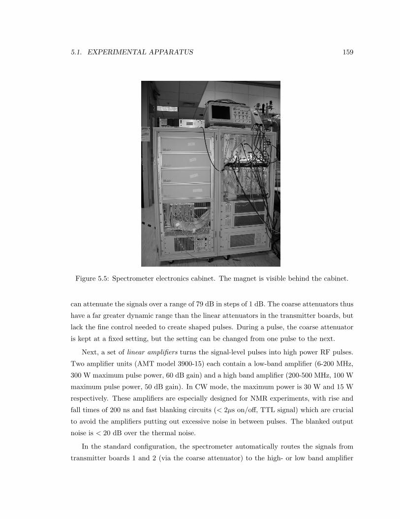
5.1. EXPERIMENTAL APPARATUS 159
Figure 5.5: Spectrometer electronics cabinet. The magnet is visible behind the cabinet.
can attenuate the signals over a range of 79 dB in steps of 1 dB. The coarse attenuators thus
have a far greater dynamic range than the linear attenuators in the transmitter boards, but
lack the fine control needed to create shaped pulses. During a pulse, the coarse attenuator
is kept at a fixed setting, but the setting can be changed from one pulse to the next.
Next, a set of linear amplifiers turns the signal-level pulses into high power RF pulses.
Two amplifier units (AMT model 3900-15) each contain a low-band amplifier (6-200 MHz,
300 W maximum pulse power, 60 dB gain) and a high band amplifier (200-500 MHz, 100 W
maximum pulse power, 50 dB gain). In CW mode, the maximum power is 30 W and 15 W
respectively. These amplifiers are especially designed for NMR experiments, with rise and
fall times of 200 ns and fast blanking circuits (< 2µs on/off, TTL signal) which are crucial
to avoid the amplifiers putting out excessive noise in between pulses. The blanked output
noise is < 20 dB over the thermal noise.
In the standard configuration, the spectrometer automatically routes the signals from
transmitter boards 1 and 2 (via the coarse attenuator) to the high- or low band amplifier

160 CHAPTER 5. EXPERIMENTAL REALIZATION
within the first dual amplifier unit, depending on whether the signals are high or low
band. Similarly, the signals from transmitter boards 3 and 4 go to the correct side of the
second dual amplifier unit. In some experiments, we have used different configurations,
using external combiners, in order to extend the routing capabilities of the spectrometer as
needed. We have also inserted stepper attenuators with a range of 1 dB and a resolution
of 0.1 dB in order to even out differences in output power between the four transmitter
boards.
The output of the two high- and low-band power amplifiers are combined as needed
with high power combiners, and then routed to the high and low band coil of the probe via
active PIN diode transmit/receive switches. In transmit mode (during the pulse sequence),
these switches connect the probe to the power amplifier output with less than 0.5 dB loss
and isolate the power amplifiers from the receiver preamplifiers (see section 5.1.5). Extra
protection for the preamplifiers is provided by quarter wave length cables and shunt diodes.
In order to attenuate broadband noise put out by the amplifiers, narrow band, high-pass
or low-pass filters are inserted between the power amplifier and the transmit/receive switch
as needed.
The pulse amplitude and duration are calibrated via a series of experiments in which
the amplitude and/or duration are systematically varied. The amplitude of the resulting
output spectra varies sinusoidally as a function of the pulse amplitude and duration. The
settings which give the first zero crossing of the output signal are the optimal 180 pulse
settings. For a 90 pulse, either the amplitude or the duration must be halved.
For the seven-qubit experiment of section 5.10, we installed an additional frequency
source (PTS 620 MHO 2YX-62), gating circuit and power amplifier (ENI model 500 LA,
1 V max input, 27 dB gain) in order to be able to send CW power at the 1H frequency
during the pulse sequence (but not during the read-out) without sacrificing any of the four
transmitter channels which were used to pulse the 19F and 13C spins. A narrow-band 1H
filter at the output of the ENI amplifier ensured a low noise level going into the probe at
the 19F and 13C frequencies.
5.1.5 Receiver
The function of the receiver is to record the voltage induced in the coil by the oscillating
magnetic signals from the spins. We have tested and used a prototype four-channel re-
ceiver system designed by Varian NMR. Conventional spectrometers have only one receiver

5.1. EXPERIMENTAL APPARATUS 161
channel.
With the transmit/receive switch in receive mode, the NMR signal is routed from the
high-band and low-band RF coils to a high- or low-band preamplifier, with a typical loss of
0.1-0.2 dB. The overall noise figure of the preamplifiers is 1.7 dB for the high band preamp
and 1.2-1.6 dB for the low band preamp, low enough such that the total noise level is
dominated by the coil rather than by the preamp. The preamp gain is about 35 dB.
The amplified RF signals are then mixed with the output of the PTS sources to an
intermediate frequency (IF) around 20 MHz. The four IF signals are routed to the receiver
boards in the electronics cabinet, where the signals are mixed with a 20 MHz signal down
to audio-frequencies, separated into two quadratures, and sent through audio filters (the
filter bandwidth can be adjusted from 1000 Hz to 256 kHz). Both quadratures are then
amplified to the desired level and digitized (the maximum number of points is 524288 and
the maximum sampling rate is 1 MHz). Finally, the digitized signals are uploaded to a
workstation.
We note that the digitized signal is phase referenced against the same frequency sources
(PTS RF sources and the 20 MHz source) as were used in the transmitter chain. For each
channel, the phase of the receiver is thus coherent with the phase of the transmitter, and
the phase of the output spectra will be exactly the same every time the same pulse sequence
is executed.
5.1.6 Workstation
The spectrometer is operated via Vnmr (Varian software) running on a Sun Ultra 10 work-
station. Once the hardware is configured properly for a certain type of experiment and
for a certain number and kind of spins, the user can set up new experiments entirely by
computer.
Pulse sequences are written in C, with additional commands such as “send a pulse on
channel 2”, provided by Varian. Such a command must be accompanied by parameters and
extra commands to specify, for example, that the pulse must last 426 µs, be phase shifted
by −29 with respect to the x axis of the oscillator reference frame (the lab frame), be
14 dB below full power, have a gaussian shaped profile, and also that it causes a 12 phase
shift on spin 4 and a −25 phase shift on spin 1, has a pre-pulse delay of 10 µs, a post-pulse
delay of 20 µs, and so forth.
For each experiment, we wrote a framework with convenient macros which can be called
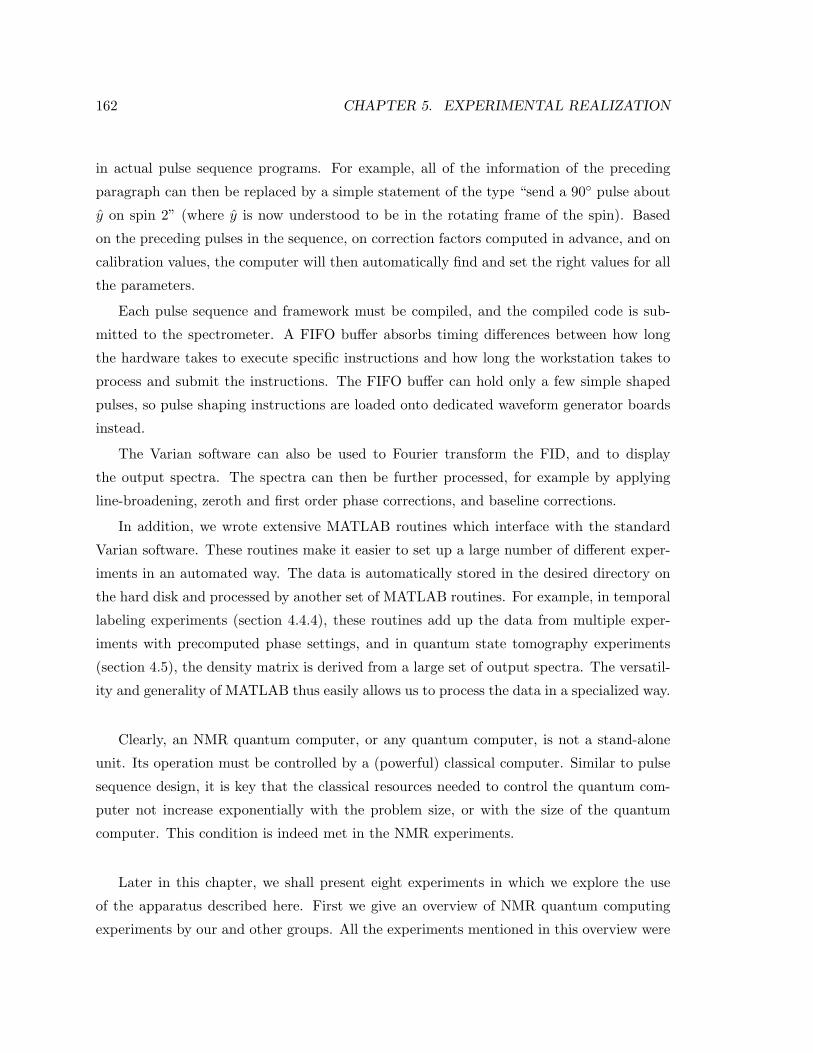
162 CHAPTER 5. EXPERIMENTAL REALIZATION
in actual pulse sequence programs. For example, all of the information of the preceding
paragraph can then be replaced by a simple statement of the type “send a 90 pulse about
y on spin 2” (where y is now understood to be in the rotating frame of the spin). Based
on the preceding pulses in the sequence, on correction factors computed in advance, and on
calibration values, the computer will then automatically find and set the right values for all
the parameters.
Each pulse sequence and framework must be compiled, and the compiled code is sub-
mitted to the spectrometer. A FIFO buffer absorbs timing differences between how long
the hardware takes to execute specific instructions and how long the workstation takes to
process and submit the instructions. The FIFO buffer can hold only a few simple shaped
pulses, so pulse shaping instructions are loaded onto dedicated waveform generator boards
instead.
The Varian software can also be used to Fourier transform the FID, and to display
the output spectra. The spectra can then be further processed, for example by applying
line-broadening, zeroth and first order phase corrections, and baseline corrections.
In addition, we wrote extensive MATLAB routines which interface with the standard
Varian software. These routines make it easier to set up a large number of different exper-
iments in an automated way. The data is automatically stored in the desired directory on
the hard disk and processed by another set of MATLAB routines. For example, in temporal
labeling experiments (section 4.4.4), these routines add up the data from multiple exper-
iments with precomputed phase settings, and in quantum state tomography experiments
(section 4.5), the density matrix is derived from a large set of output spectra. The versatil-
ity and generality of MATLAB thus easily allows us to process the data in a specialized way.
Clearly, an NMR quantum computer, or any quantum computer, is not a stand-alone
unit. Its operation must be controlled by a (powerful) classical computer. Similar to pulse
sequence design, it is key that the classical resources needed to control the quantum com-
puter not increase exponentially with the problem size, or with the size of the quantum
computer. This condition is indeed met in the NMR experiments.
Later in this chapter, we shall present eight experiments in which we explore the use
of the apparatus described here. First we give an overview of NMR quantum computing
experiments by our and other groups. All the experiments mentioned in this overview were

5.2. OVERVIEW OF NMR QUANTUM COMPUTING EXPERIMENTS 163
done using an apparatus similar to ours.
5.2 Overview of NMR quantum computing experiments
Nuclear magnetic resonance spectroscopy, invented in 1946, developed from a method to
study magnetism into a powerful and versatile tool for the study of molecular structure
and reaction dynamics. The first 25 years of NMR were dominated by CW slow passage
experiments. In the 1970’s, pulsed Fourier transform spectroscopy was developed, which led
to an unprecedented expansion of the field and its applications. Many of the pulsed NMR
protocols have a structure which we now recognize is similar to quantum computing pulse
sequences; for example, the INEPT pulse sequence for polarization transfer is in essence the
same as the sequence for a cnot gate.
Only in the last four years have researchers begun to implement NMR pulse sequences
with the explicit purpose of studying quantum computation. Several groups besides our
own have pursued liquid NMR quantum computing very actively and they continue to
implement a variety of quantum information processing tasks. We will now give a very brief
overview of this work.
Quantum algorithms
The first quantum algorithms ever implemented experimentally were Grover’s algorithm
for two qubits [CGK98, JMH98] and the Deutsch-Jozsa algorithm for two qubits [CVZ+98,
JM98] (section 5.3). These experiments were performed in the Fall of 1997 and Winter of
1998, by Ike Chuang’s group at UC Berkeley and Stanford University using the 13C and1H spins of 13C-labeled chloroform and in Jonathan Jones’s lab at Oxford University using
two two 1H spins of cytosine.
Later, the quantum counting algorithm (an extension of Grover’s search algorithm) was
also implemented on the two spins of cytosine [JM99]. The two-qubit Grover algorithm was
implemented again on a subspace of two spins out of the three 19F spins of bromotrifluo-
roethylene, in the first demonstration of logical labeling [VYSC99] (section 5.5). Finally, the
three-qubit Grover algorithm was realized using the 1H-13C-19F spin system of dibromoflu-
oromethane; up to 28 Grover iterations, involving a record 280 two-qubit gates [VSS+00]
(section 5.7).
The Deutsch-Jozsa algorithm for three qubits was implemented in Ray Freeman’s lab at

164 CHAPTER 5. EXPERIMENTAL REALIZATION
Cambridge University using the three 1H nuclei in 2,3-dibromoproponic acid, and exploring
the use of transition selective pulses [LBF98]. The same molecule was used again later in a
similar experiment [DAK00]. A more advanced version of the algorithm was demonstrated
using the three 13C nuclei in fully labeled alanine, and swap gates to realize two-qubit
gates between the two weakly coupled 13C spins [CKH+00]. The same molecule was used
without swap gates for another three-qubit Deutsch-Jozsa experiment [KLL00]. A partial
(particularly simple) implementation of the five-qubit Deutsch-Jozsa algorithm was carried
out using one 1H, 15N and 19F nucleus and two 13C nuclei in a molecule derived from
glycine [MFM+00]. This experiment, done by Steffen Glaser’s group in Franfurt, was the
first demonstration of coherent control over five qubits.
The implementation of quantum algorithms was taken to a new level of complexity
by the first implementation of a Shor-type quantum algorithm for order-finding on a five-
fluorine spin system, carried out at IBM/Stanford [VSB+00] (section 5.9). This algorithm
combined exponentiated permutations with the three-qubit quantum Fourier transform; the
latter had been implemented earlier in itself using 13C labeled alanine [WPF+01]. The five-
qubit experiment was followed by a seven-qubit demonstration, also at IBM/Stanford, of
the simplest instance of Shor’s quantum factoring algorithm, the prime factorization of the
number 15 [VSB+01] (section 5.10).
Quantum error correction
The first demonstration of quantum error correction was done using alanine and trichloro-
ethylene, in David Cory’s group at MIT/Harvard and by Raymand Laflamme and Em-
manual Knill at Los Alamos [CMP+98]. They implemented the three-qubit phase error
correction code and studied its operation for one particular input state in the presence of
gradient fields to introduce artifical errors, and also when subject to just intrinsic decoher-
ence. A more complete version of this experiment was carried out later by the same groups,
using gradient fields [SCS+00]. Meanwhile, a complete experiment for the two-bit phase er-
ror detection code had been implemented by our group, for intrinsic decoherence [LVZ+99]
(section 5.4). Recently, the Los Alamos group demonstrated the five-bit phase and am-
plitude error correction code for full bit and phase flip errors that were artificially intro-
duced [KLMN01].

5.2. OVERVIEW OF NMR QUANTUM COMPUTING EXPERIMENTS 165
Quantum simulations
Relatively little but very interesting work has been done on quantum simulations. David
Cory’s group first simulated the dynamics of truncated quantum harmonic and anharmonic
oscillators, using the two proton spins of 2,3-dibromothiophene [STH+99]. Later, the same
group simulated a non-physical three-body interaction using the three carbon spins in fully
labeled alanine [TSS+99].
Other quantum protocols
The group at Los Alamos prepared an effective pure GHZ state (a GHZ state is a maximally
entangled state of three particles) [LKZ+98], and later performed a similar experiment on
seven spins [KLMT00]. Even though the claim that entangled states or cat states had been
prepared has been refuted on the basis that the spin states at room temperature are too
mixed to be entangled [BCJ+99] (rather than entangled states, a three spin and seven spin
coherence has been observed), these experiments remain the first, albeit relatively simple,
experiments with three respectively seven qubits. GHZ correlations on mixed states have
been studied further in an experiment by the MIT group [NCL00].
Also at Los Alamos, a teleportation protocol has been carried out using two 13C nuclei
and one 1H nucleus in 13C labeled trichloroethylene [NKL98]. Superdense coding was
also demonstrated, with 13C labeled chloroform [FZF+00]. Just like the work on pseudo-
entangled states, the significance of these experiments is limited by the mixedness of the
states and furthermore by the fact that the nuclei are separated from each other by only a
few Angstroms.
Polarization enhancement
It is clear that the tiny polarizations obtained for nuclear spins in thermal equilibrium
at room temperature severely limit the usefulness of NMR quantum computers. Several
experiments have been done to study the feasability of boosting the nuclear spin polar-
ization. In an algorithmic approach, the building block of the Schulman-Vazirani cooling
scheme has been demonstrated at IBM/Stanford using the three fluorine spins of bromotri-
fluoroethylene [CVS01] (section 5.8). However, this scheme is impractical as long as the
starting polarization remains very low. Also at IBM/Stanford, the initial polarization of
the 1H and 13C spins in labeled chloroform has been increased by a factor of about 10 using
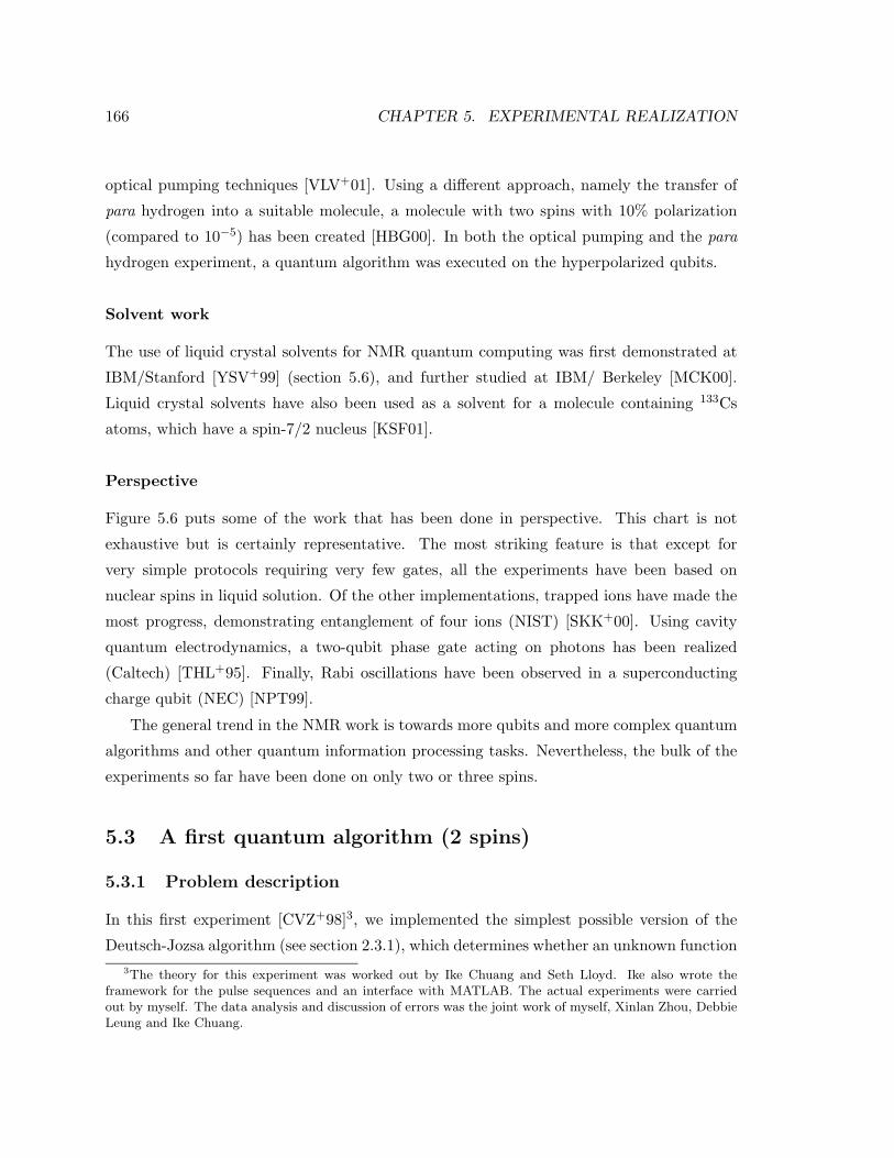
166 CHAPTER 5. EXPERIMENTAL REALIZATION
optical pumping techniques [VLV+01]. Using a different approach, namely the transfer of
para hydrogen into a suitable molecule, a molecule with two spins with 10% polarization
(compared to 10−5) has been created [HBG00]. In both the optical pumping and the para
hydrogen experiment, a quantum algorithm was executed on the hyperpolarized qubits.
Solvent work
The use of liquid crystal solvents for NMR quantum computing was first demonstrated at
IBM/Stanford [YSV+99] (section 5.6), and further studied at IBM/ Berkeley [MCK00].
Liquid crystal solvents have also been used as a solvent for a molecule containing 133Cs
atoms, which have a spin-7/2 nucleus [KSF01].
Perspective
Figure 5.6 puts some of the work that has been done in perspective. This chart is not
exhaustive but is certainly representative. The most striking feature is that except for
very simple protocols requiring very few gates, all the experiments have been based on
nuclear spins in liquid solution. Of the other implementations, trapped ions have made the
most progress, demonstrating entanglement of four ions (NIST) [SKK+00]. Using cavity
quantum electrodynamics, a two-qubit phase gate acting on photons has been realized
(Caltech) [THL+95]. Finally, Rabi oscillations have been observed in a superconducting
charge qubit (NEC) [NPT99].
The general trend in the NMR work is towards more qubits and more complex quantum
algorithms and other quantum information processing tasks. Nevertheless, the bulk of the
experiments so far have been done on only two or three spins.
5.3 A first quantum algorithm (2 spins)
5.3.1 Problem description
In this first experiment [CVZ+98]3, we implemented the simplest possible version of the
Deutsch-Jozsa algorithm (see section 2.3.1), which determines whether an unknown function3The theory for this experiment was worked out by Ike Chuang and Seth Lloyd. Ike also wrote the
framework for the pulse sequences and an interface with MATLAB. The actual experiments were carriedout by myself. The data analysis and discussion of errors was the joint work of myself, Xinlan Zhou, DebbieLeung and Ike Chuang.
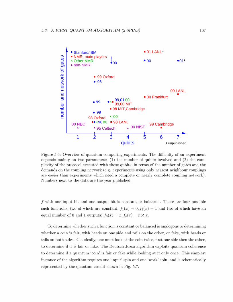
5.3. A FIRST QUANTUM ALGORITHM (2 SPINS) 167
num
ber
and
netw
ork
of g
ates
Stanford/IBM
Other NMRNMR, main players
non-NMR
1 2 3 4 5 6 7
99
01
qubits
99 Cambridge
98 MIT,Cambridge
00 Frankfurt
00
99,0199,00 MIT
00
98 LANL
99
00 NIST95 Caltech00 NEC
98 Oxford
00 LANL
99 Oxford98
01 LANL
9800
00 00
*
*
unpublished*
Figure 5.6: Overview of quantum computing experiments. The difficulty of an experimentdepends mainly on two parameters: (1) the number of qubits involved and (2) the com-plexity of the protocol executed with those qubits, in terms of the number of gates and thedemands on the coupling network (e.g. experiments using only nearest neighbour couplingsare easier than experiments which need a complete or nearly complete coupling network).Numbers next to the data are the year published.
f with one input bit and one output bit is constant or balanced. There are four possible
such functions, two of which are constant, f1(x) = 0, f2(x) = 1 and two of which have an
equal number of 0 and 1 outputs: f3(x) = x, f4(x) = not x.
To determine whether such a function is constant or balanced is analogous to determining
whether a coin is fair, with heads on one side and tails on the other, or fake, with heads or
tails on both sides. Classically, one must look at the coin twice, first one side then the other,
to determine if it is fair or fake. The Deutsch-Jozsa algorithm exploits quantum coherence
to determine if a quantum ‘coin’ is fair or fake while looking at it only once. This simplest
instance of the algorithm requires one ‘input’ spin and one ‘work’ spin, and is schematically
represented by the quantum circuit shown in Fig. 5.7.
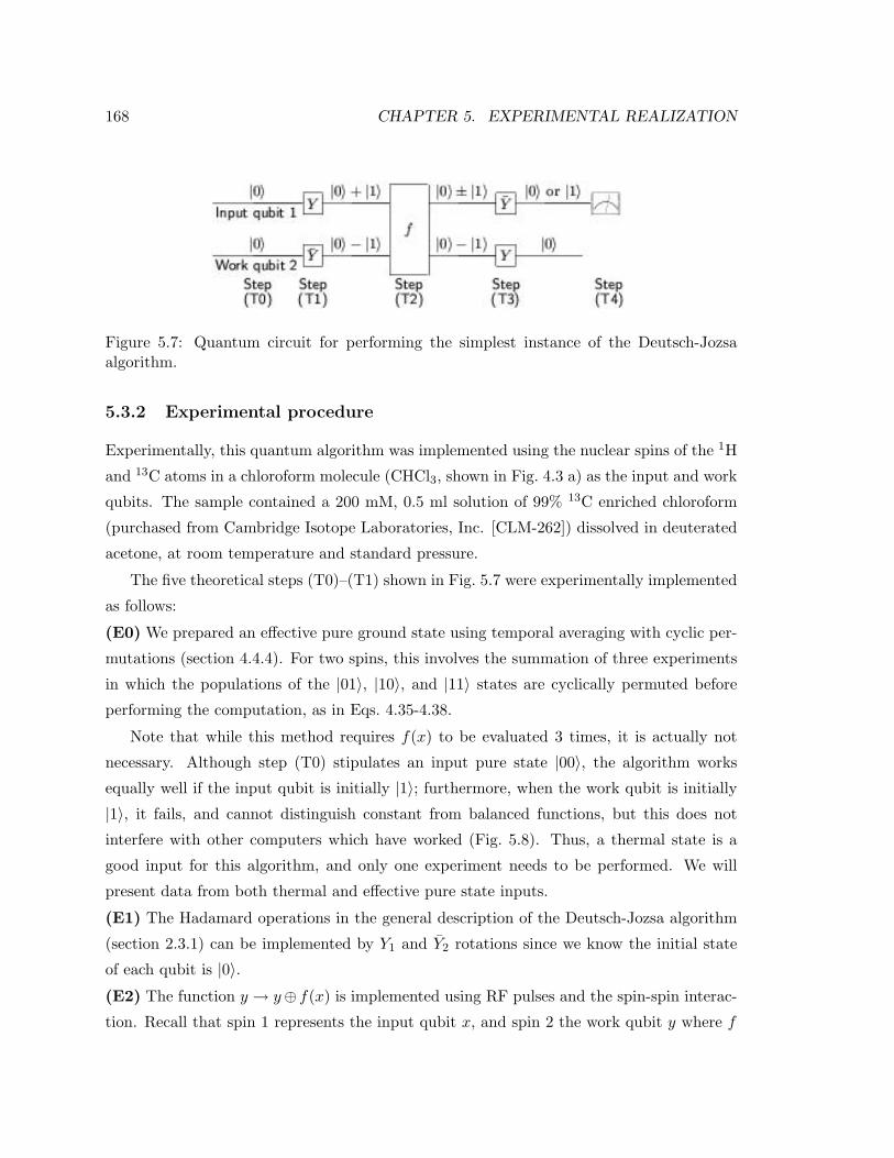
168 CHAPTER 5. EXPERIMENTAL REALIZATION
Figure 5.7: Quantum circuit for performing the simplest instance of the Deutsch-Jozsaalgorithm.
5.3.2 Experimental procedure
Experimentally, this quantum algorithm was implemented using the nuclear spins of the 1H
and 13C atoms in a chloroform molecule (CHCl3, shown in Fig. 4.3 a) as the input and work
qubits. The sample contained a 200 mM, 0.5 ml solution of 99% 13C enriched chloroform
(purchased from Cambridge Isotope Laboratories, Inc. [CLM-262]) dissolved in deuterated
acetone, at room temperature and standard pressure.
The five theoretical steps (T0)–(T1) shown in Fig. 5.7 were experimentally implemented
as follows:
(E0) We prepared an effective pure ground state using temporal averaging with cyclic per-
mutations (section 4.4.4). For two spins, this involves the summation of three experiments
in which the populations of the |01〉, |10〉, and |11〉 states are cyclically permuted before
performing the computation, as in Eqs. 4.35-4.38.
Note that while this method requires f(x) to be evaluated 3 times, it is actually not
necessary. Although step (T0) stipulates an input pure state |00〉, the algorithm works
equally well if the input qubit is initially |1〉; furthermore, when the work qubit is initially
|1〉, it fails, and cannot distinguish constant from balanced functions, but this does not
interfere with other computers which have worked (Fig. 5.8). Thus, a thermal state is a
good input for this algorithm, and only one experiment needs to be performed. We will
present data from both thermal and effective pure state inputs.
(E1) The Hadamard operations in the general description of the Deutsch-Jozsa algorithm
(section 2.3.1) can be implemented by Y1 and Y2 rotations since we know the initial state
of each qubit is |0〉.(E2) The function y → y⊕ f(x) is implemented using RF pulses and the spin-spin interac-
tion. Recall that spin 1 represents the input qubit x, and spin 2 the work qubit y where f
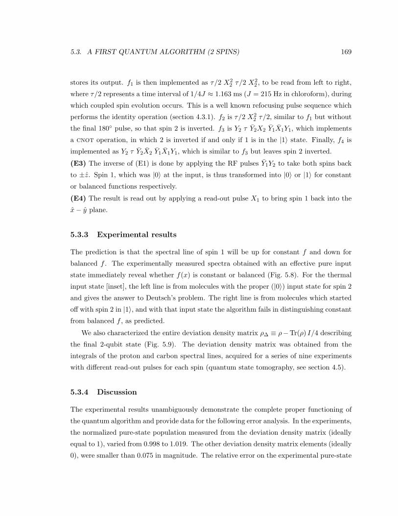
5.3. A FIRST QUANTUM ALGORITHM (2 SPINS) 169
stores its output. f1 is then implemented as τ/2 X22 τ/2 X
22 , to be read from left to right,
where τ/2 represents a time interval of 1/4J ≈ 1.163 ms (J = 215 Hz in chloroform), during
which coupled spin evolution occurs. This is a well known refocusing pulse sequence which
performs the identity operation (section 4.3.1). f2 is τ/2 X22 τ/2, similar to f1 but without
the final 180 pulse, so that spin 2 is inverted. f3 is Y2 τ Y2X2 Y1X1Y1, which implements
a cnot operation, in which 2 is inverted if and only if 1 is in the |1〉 state. Finally, f4 is
implemented as Y2 τ Y2X2 Y1X1Y1, which is similar to f3 but leaves spin 2 inverted.
(E3) The inverse of (E1) is done by applying the RF pulses Y1Y2 to take both spins back
to ±z. Spin 1, which was |0〉 at the input, is thus transformed into |0〉 or |1〉 for constant
or balanced functions respectively.
(E4) The result is read out by applying a read-out pulse X1 to bring spin 1 back into the
x− y plane.
5.3.3 Experimental results
The prediction is that the spectral line of spin 1 will be up for constant f and down for
balanced f . The experimentally measured spectra obtained with an effective pure input
state immediately reveal whether f(x) is constant or balanced (Fig. 5.8). For the thermal
input state [inset], the left line is from molecules with the proper (|0〉) input state for spin 2
and gives the answer to Deutsch’s problem. The right line is from molecules which started
off with spin 2 in |1〉, and with that input state the algorithm fails in distinguishing constant
from balanced f , as predicted.
We also characterized the entire deviation density matrix ρ∆ ≡ ρ−Tr(ρ) I/4 describing
the final 2-qubit state (Fig. 5.9). The deviation density matrix was obtained from the
integrals of the proton and carbon spectral lines, acquired for a series of nine experiments
with different read-out pulses for each spin (quantum state tomography, see section 4.5).
5.3.4 Discussion
The experimental results unambiguously demonstrate the complete proper functioning of
the quantum algorithm and provide data for the following error analysis. In the experiments,
the normalized pure-state population measured from the deviation density matrix (ideally
equal to 1), varied from 0.998 to 1.019. The other deviation density matrix elements (ideally
0), were smaller than 0.075 in magnitude. The relative error on the experimental pure-state

170 CHAPTER 5. EXPERIMENTAL REALIZATION
Figure 5.8: Proton spectrum after completion of the Deutsch-Jozsa algorithm and a singleread-out pulse X1, with an effectively pure input state |00〉 and with a thermal inputstate [Inset]. The low (high) frequency lines correspond to the transitions |00〉 ↔ |10〉(|01〉 ↔ |11〉). The frequency is relative to ω1
0 (the Larmor frequency of spin 1), and theamplitude has arbitrary units. The phase is set such that a spectral line is real and positive(negative) when spin 1 is |0〉 (|1〉) right before the read-out pulse.
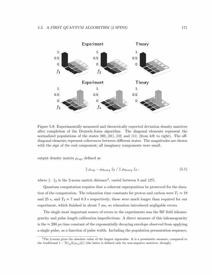
5.3. A FIRST QUANTUM ALGORITHM (2 SPINS) 171
0
0.5
1
0
0.5
1
0
0.5
1
0
0.5
1
0
0.5
1
0
0.5
1
Figure 5.9: Experimentally measured and theoretically expected deviation density matricesafter completion of the Deutsch-Jozsa algorithm. The diagonal elements represent thenormalized populations of the states |00〉, |01〉, |10〉 and |11〉 (from left to right). The off-diagonal elements represent coherences between different states. The magnitudes are shownwith the sign of the real component; all imaginary components were small.
output density matrix ρexp, defined as
‖ ρexp − ρtheory ‖2 / ‖ ρtheory ‖2 , (5.1)
where ‖ · ‖2 is the 2-norm matrix distance4, varied between 8 and 12%.
Quantum computation requires that a coherent superposition be preserved for the dura-
tion of the computation. The relaxation time constants for proton and carbon were T1 ≈ 19
and 25 s, and T2 ≈ 7 and 0.3 s respectively; these were much longer than required for our
experiment, which finished in about 7 ms, so relaxation introduced negligable errors.
The single most important source of errors in the experiments was the RF field inhomo-
geneity and pulse length calibration imperfections. A direct measure of this inhomogeneity
is the ≈ 200 µs time constant of the exponentially decaying envelope observed from applying
a single pulse, as a function of pulse width. Including the population permutation sequence,
4The 2-norm gives the absolute value of the largest eigenvalue. It is a pessimistic measure, compared tothe traditional 1− Tr(
√ρ1ρ2√ρ1) (the latter is defined only for non-negative matrices, though).
172 CHAPTER 5. EXPERIMENTAL REALIZATION
about 7 pulses are applied to each nucleus, with a cumulative duration of ≈ 70− 100µs.
The second most important contribution to errors is the low carbon signal-to-noise ratio:
the carbon signal peak height/RMS noise was about 35, versus ≈ 4300 for the proton. The
carbon signal was much weaker because the carbon gyromagnetic ratio is 4 times smaller,
and the carbon receiver coil is mounted farther away from the sample. Smaller contributions
to errors came from incomplete thermalization between subsequent experiments, carrier
frequency offsets, and numerical errors in the data analysis.
In summary, the quantum computation succeeded, and the quantum computer solved a
problem in fewer steps than is possible classically. Furthermore, for this small-scale quantum
computer, imperfections were dominated by technology, rather than by fundamental issues.
5.4 Quantum error detection (2 spins)
5.4.1 Problem description
The goal of this experiment [LVZ+99]5 was to study the effectiveness of quantum error
correction in a real experimental system, focusing on effects arising from imperfections of
the logic gates. We did this by testing the two-qubit error detection code of section 2.4.1
on a two-spin molecule.
We designed the experiment such that potential artificial origins of (favorable) bias
were eliminated in the following ways. First, we compared the preservation of arbitrary
states stored with and without coding (the latter is unprotected but not affected by coding
operations). Second, by ensuring that all qubits used in the code decohere at nearly the
same rate, we eliminated apparent improvements brought about by having an ancilla with
a lifetime much longer than the original unencoded qubit. Third, our experiment utilized
only naturally occurring error processes.
5.4.2 Experimental procedure
The molecule selected for this experiment was 13C-labeled sodium formate (CHOO−Na+)
at 15C. The sample was a 0.6 ml, 1.26 molar solution (8:1 molar ratio with anhydrous
calcium chloride) in deuterated water. The proton and carbon were used as input (qubit5This experiment was proposed by Debbie Leung and Ike Chuang. They also worked out the theory. Sam-
ples were selected and prepared by Mark Sherwood and Nino Yannoni. I performed the actual experiment.The data analysis and numerical simulations were mostly the work of Debbie, Ike and Xinlan Zhou.
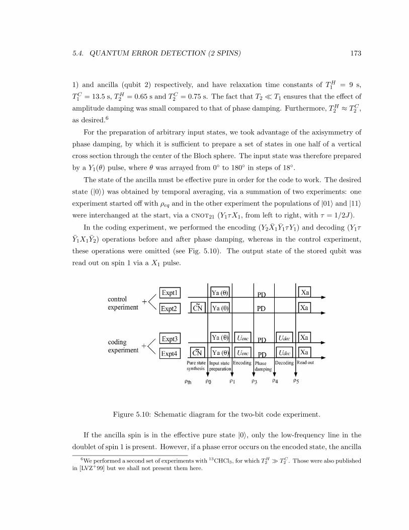
5.4. QUANTUM ERROR DETECTION (2 SPINS) 173
1) and ancilla (qubit 2) respectively, and have relaxation time constants of TH1 = 9 s,
TC1 = 13.5 s, TH2 = 0.65 s and TC2 = 0.75 s. The fact that T2 T1 ensures that the effect of
amplitude damping was small compared to that of phase damping. Furthermore, TH2 ≈ TC2 ,
as desired.6
For the preparation of arbitrary input states, we took advantage of the axisymmetry of
phase damping, by which it is sufficient to prepare a set of states in one half of a vertical
cross section through the center of the Bloch sphere. The input state was therefore prepared
by a Y1(θ) pulse, where θ was arrayed from 0 to 180 in steps of 18.
The state of the ancilla must be effective pure in order for the code to work. The desired
state (|0〉) was obtained by temporal averaging, via a summation of two experiments: one
experiment started off with ρeq and in the other experiment the populations of |01〉 and |11〉were interchanged at the start, via a cnot21 (Y1τX1, from left to right, with τ = 1/2J).
In the coding experiment, we performed the encoding (Y2X1Y1τY1) and decoding (Y1τ
Y1X1Y2) operations before and after phase damping, whereas in the control experiment,
these operations were omitted (see Fig. 5.10). The output state of the stored qubit was
read out on spin 1 via a X1 pulse.
Figure 5.10: Schematic diagram for the two-bit code experiment.
If the ancilla spin is in the effective pure state |0〉, only the low-frequency line in the
doublet of spin 1 is present. However, if a phase error occurs on the encoded state, the ancilla6We performed a second set of experiments with 13CHCl3, for which TH2 TC2 . Those were also published
in [LVZ+99] but we shall not present them here.

174 CHAPTER 5. EXPERIMENTAL REALIZATION
will be |1〉 after decoding. Thus, after decoding, the low-frequency line of the doublet of spin
1 corresponds to “accepted” states and the high-frequency line corresponds to “rejected”
states.
5.4.3 Experimental results
The predicted accepted output states with and without coding are shown in Fig. 5.11.
These plots are the result of numerical simulations which include the phase damping model
of Eq. 3.26 in section 3.1.5. The main feature is that the Bloch sphere becomes ellipsoidal
without encoding but remains largely spherical (i.e. the state is better preserved) with
encoding. We note that the amplitude of the accepted states is shrunk with respect to the
original state; this is because the two-bit code can only detect, not correct errors.
0 0.25 0.5 0.75 1
−1
−0.75
−0.5
−0.25
0
0.25
0.5
0.75
1|0>
|1>
x−axis of Bloch sphere
z−ax
is o
f Blo
ch s
pher
e
0 0.25 0.5 0.75 1
−1
−0.75
−0.5
−0.25
0
0.25
0.5
0.75
1|0>
|1>
x−axis of Bloch sphere
z−ax
is o
f Blo
ch s
pher
e
Figure 5.11: Predicted Bloch spheres (a) with and (b) without encoding, for a set of equallyspaced storage times (k×61.5 ms for k = 0, 1 . . . ,5), corresponding to a probability of phaseerror (without encoding) of p = 0, 0.071, 0.133, 0.185, 0.230 and 0.269.
Figure 5.12 shows the experimentally measured accepted output states, again with and
without coding. The agreement of the main features between Figs. 5.11 and 5.12 is striking.

5.4. QUANTUM ERROR DETECTION (2 SPINS) 175
0 0.25 0.5 0.75 1
−1
−0.75
−0.5
−0.25
0
0.25
0.5
0.75
1|0>
|1>
x−axis of Bloch sphere
z−ax
is o
f Blo
ch s
pher
e
t = 0
t = 61.5
0 0.25 0.5 0.75 1
−1
−0.75
−0.5
−0.25
0
0.25
0.5
0.75
1|0>
|1>
x−axis of Bloch sphere
z−ax
is o
f Blo
ch s
pher
e
t = 61.5
t = 0
Figure 5.12: Experimentally measured Bloch spheres (a) with and (b) without encoding,for the same storage times as in Fig. 5.11. The circles are experimental data points and thesolid lines are least square fitted ellipses.
5.4.4 Discussion
We quantified how well a quantum state is preserved experimentally via the ellipticity of
the Bloch sphere, which we define as √I(θ = 0)I(θ = π
2 )(5.2)
where the intensity I as a function of θ is ideally of the form
Iideal(θ) = A+B sin2 θ . (5.3)
In order to include signal strength attenuation with increasing θ and constant offsets in
the angular positions, we actually fitted (non-linear least-squares fit) the experimental data

176 CHAPTER 5. EXPERIMENTAL REALIZATION
points to the expression
Iexp(θ) = (A+B sin2(θ +D))(1− C(θ +D)) (5.4)
instead.
0 50 100 150 200 250 300 3500.8
1
1.2
1.4
1.6
1.8
2
2.2
2.4
2.6
Storage time [ms]
Elli
ptic
ity
w/o codingw/t codingideal simulation
Figure 5.13: Ellipticity as a function of storage time. The experimental datapoints are givenfor the case with and without coding, along with ideal predictions as well as simulationswhich take the effect of RF inhomogeneities into account.
The data of Fig. 5.13 demonstrate that coding removes the first order term in the growth
of the Bloch sphere ellipticity as a function of storage time, which corresponds to the first
order improvement in the conditional fidelity expected from the theory (section 2.4.1).
However, imperfections in the logic gates caused the ellipticity to increase by 10% for the
case of zero storage time (i.e. the zeroth order term). This number represents the cost of
“noisy” gates.
While the data of Fig. 5.12 exhibit a clear correction effect, there are notable deviations
from the ideal case of Fig. 5.11. First, the ellipses with coding are smaller than their

5.5. LOGICAL LABELING (3 SPINS) 177
counterparts without coding (this reduces the absolute fidelity but not the conditional
fidelity). This is most obvious when the storage time is zero, in which case the coding
and the control experiments should produce equal outputs. Second, the signal strength
is attenuated with increasing θ relative to ideal ellipses. Third, although the data points
are well fitted by ellipses, their angular positions are not exactly as expected (“θ-offsets”).
Finally, the spacings between the ellipses deviate from expectation.
A major cause of experimental errors was RF field inhomogeneity, which causes gate
imperfections. This was determined by a series of simulations of RF inhomogeneity effects,
which reproduced the reduced amplitude in the coding experiments. The asymmetry in
the experimental Bloch spheres is well explained by amplitude damping. We do not have a
convincing explanation for the other two discrepancies.
In summary, we have demonstrated experimentally that using a two bit phase damping
detection code, the coherence time of qubits in bulk NMR systems can be conditionally
lengthened. These experimental results also provide quantitative measures of the major
imperfections in the system. The principle source of errors, RF field inhomogeneity, was
studied and a numerical simulation was developed to model our data. Despite the imper-
fections, a net amount of error reduction was observed, when comparing cases with and
without coding, including gate errors in both cases.
5.5 Logical labeling (3 spins)
5.5.1 Problem description
The goal of this experiment [VYSC99]7 was threefold: (1) to take a step in complexity from
two spins to three spins, (2) to explore the use of homonuclear spin systems and (3) to test
the concept of logical labeling for the first time. These three goals come together naturally
as at least three spins are required for a meaningful demonstration of logical labeling, and
all three spins must be homonuclear (section 4.4.3).
The operations needed for logical labeling follow from comparison of Eq. 4.32 with
7This experiment was proposed by myself. I also worked out the theory, wrote the framework for dealingwith homonuclear spins, invented the “uncoupling frame” wrote the pulse sequences, carried out the experi-ment and did the data analysis, under the guidance of Ike Chuang. Nino Yannoni and Mark Sherwood cameup with the molecule, prepared the sample and gave advice on NMR techniques.

178 CHAPTER 5. EXPERIMENTAL REALIZATION
Eq. 4.33: the populations of the states |001〉 ↔ |101〉 and |010〉 ↔ |110〉 must be inter-
changed, while the remaining four populations must be unaffected. This requires a cnot21
and a cnot31.
As a test of logical labeling and subsequent control over the dynamical behavior of
the logically labeled spins, we chose to implement Grover’s algorithm on the effective pure
two-qubit subspace within the three-spin molecule. With the two-qubit version of this al-
gorithm, one can find the unique but unknown x0 among N = 4 possible values of x which
satisfies f(x0) = 1 in just one query, compared to on average 2.25 queries classically.
A fourth, additional, goal was to study the preservation of the effective pure state after
many operations. Grover’s algorithm lends itself perfectly to such studies in the form of
many repeated Grover iterations (section 2.3.2).
5.5.2 Experimental procedure
We selected bromotrifluoroethylene (Fig. 4.3 c) dissolved in deuterated acetone (10 mol%)
as the central molecule in our experiments, because the spin-1/2 19F nuclei have large J-
couplings and chemical shifts, as well as long coherence times, which make it suitable for
quantum computation. The 12C nuclei are non-magnetic and the interaction of the spin-3/2
Br nucleus with the fluorine spins is averaged out due to fast Br relaxation (chapter 4).
The 19F Larmour frequencies are ≈ 470 MHz (at 11.7 T) and the spectrum is first order,
consisting of three well-separated quadruplets, with ω1−ω2/2π ≈ 13.2 kHz and ω3−ω1/2π ≈9.5 kHz. The coupling constants are measured to be J12 = −122.1 Hz, J13 = 75.0 Hz and
J23 = 53.8 Hz (see also [EM62]). In order to simultaneously address the four lines in one
quadruplet without affecting the other two quadruplets, the envelope of the RF pulses was
Gaussian shaped and the RF power was adjusted to obtain pulses of ≈ 300µs.
The two cnot gates of the logical labeling step commute and can thus be executed
simultaneously. This was done via the pulse sequence of Fig. 5.14. This sequence implements
the cnot gates only up to single-spin Z rotations, which suffices for a diagonal initial state
as used here. Furthermore, the I2z , I3
z and I2z I
3z terms in the Hamiltonian have no effect,
since spins 2 and 3 remain along ±z. I1z can be ignored because the pulses were applied in
a reference frame in resonance with each spin.
After logical labeling, the state must remain effective pure throughout the subsequent
computation. This requires that while a computation is carried out using spins 2 and 3,
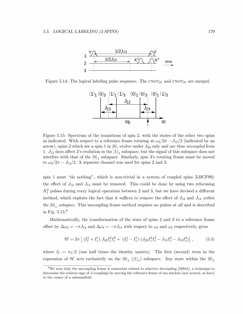
5.5. LOGICAL LABELING (3 SPINS) 179
1
2
3
1/2J13
121/2J
Y Y
XX2 2time
Figure 5.14: The logical labeling pulse sequence. The cnot21 and cnot31 are merged.
J23
J12
J23
ω2
0 3 1310 3
ω
1 1 1 311 1 0 0
Figure 5.15: Spectrum of the transitions of spin 2, with the states of the other two spinsas indicated. With respect to a reference frame rotating at ω2/2π −J12/2 (indicated by anarrow), spins 2 which see a spin 1 in |0〉, evolve under J23 only and are thus uncoupled from1. J12 does affect 2’s evolution in the |1〉1 subspace, but the signal of this subspace does notinterfere with that of the |0〉1 subspace. Similarly, spin 3’s rotating frame must be movedto ω3/2π − J13/2. A separate channel was used for spins 2 and 3.
spin 1 must “do nothing”, which is non-trivial in a system of coupled spins [LBCF99]:
the effect of J12 and J13 must be removed. This could be done by using two refocusing
X21 pulses during every logical operation between 2 and 3, but we have devised a different
method, which exploits the fact that it suffices to remove the effect of J12 and J13 within
the |0〉1 subspace. This uncoupling frame method requires no pulses at all and is described
in Fig. 5.15.8
Mathematically, the transformation of the state of spins 2 and 3 to a reference frame
offset by ∆ω2 = −πJ12 and ∆ω3 = −πJ13 with respect to ω2 and ω3 respectively, gives
H′ = 2π[
(I1I + I1
z ) J23I2z I
3z + (I1
I − I1z ) (J23I
2z I
3z − J12I
2z − J13I
3z )], (5.5)
where II = σI/2 (one half times the identity matrix). The first (second) term in the
expression of H′ acts exclusively on the |0〉1 (|1〉1) subspace. Any state within the |0〉18We note that the uncoupling frame is somewhat related to selective decoupling [ME61], a technique to
determine the relative sign of J-couplings by moving the reference frame of one nucleus (not several, as here)to the center of a submanifold.

180 CHAPTER 5. EXPERIMENTAL REALIZATION
subspace evolves only under J23I2z I
3z and will remain within the |0〉1 subspace. Within the
|0〉1 subspace and using the uncoupling reference frame, spins 2 and 3 are thus uncoupled
from 1.
For the implementation of the Grover algorithm on the logically labeled spins in the
uncoupling frame, we used a pulse sequence similar to the one described in [CGK98]. First,
Y2Y3 rotates both spins from |00〉 into (|00〉+ |01〉+ |10〉+ |11〉)/2, an equal superposition of
the four possible inputs. The amplitude of the |x0〉 term is then amplified in two steps (see
section 2.3.2). First, one of four functions fx0(x) is evaluated, flipping the sign of the |x0〉term. This is done by one of four conditional phase flips Y2Y4 Φ2Θ3 Y2Y3 1/2J23, where
Φ = X for f00 and f10 and Φ = X for f01 and f11. Θ = X for f00 and f01 and Θ = X for f10
and f11. Second, inversion about the average is implemented by a Hadamard gate on both
spins, followed by the conditional phase flip corresponding to f00, and another Hadamard
gate. The pulse sequence for this inversion step can be reduced to X2X3 Y2Y3 1/2J23 Y2Y3.
The entire sequence for Grover’s algorithm takes approximately 20 ms and the labeling
step takes about 7 ms. The coherence time for the three 19F spins, expressed as the measured
transverse relaxation time constant T2 ≈ 4-8 s, is sufficiently long for coherence to be
maintained throughout the labeling and computation operations.
5.5.3 Experimental results
Fig. 5.16 shows the measured populations of the eight basis states, before and after the se-
quence of Fig. 5.14. The results agree with the theoretical predictions of Eqs. 4.32 and 4.33.
000 001 010 011 100 101 110 111−3
0
3
000 001 010 011 100 101 110 111−3
0
3
Figure 5.16: Experimentally determined populations (in arbitrary units, and relative to theaverage) of the states |000〉, . . . , |111〉 (Left) in thermal equilibrium and (Right) after logicallabeling. The populations were determined by partial state tomography [CGKL98].
We experimentally confirmed that spins 2 and 3 are uncoupled from spin 1 by recon-
structing the deviation density matrix of the three-spin system after creating the state

5.5. LOGICAL LABELING (3 SPINS) 181
(|00〉+ |11〉)/√
2 in the |0〉1 subspace. For this three spin system, quantum state tomogra-
phy involved a series of 27 consecutive experiments with different sets of read-out pulses.
Fig. 5.17 shows the |0〉1 subsystem in the predicted effective pure state and uncoupled from
the |1〉1 subspace. The relative error in the state is ‖ ρexp − ρth ‖2/‖ ρth ‖2 = 19 %.
000001
010011
100101
110111
0
0.25
0.5
Figure 5.17: Normalized experimental deviation density matrix (with the diagonal shiftedto obtain unit trace for the effective pure state), shown in absolute value. The entries in thesecond quadrant are very small, which means that the |0〉1 and |1〉1 subspaces are uncoupled.The four density matrix elements which stick out (in the first quadrant) are, in the logicallylabeled subspace, the |00〉〈00| and |11〉〈11| entries (which represent populations) and the|00〉〈11| and|11〉〈00| entries (which represent double quantum coherences).
The theoretical prediction for the Grover algorithm is that the output state of qubits 2
and 3 is the (effective pure) state |x0〉. This can be determined by a measurement of spins
2 and 3 after a read-out pulse on each spin. The experimental spectra (Fig. 5.18, Left) as
well as the deviation density matrices of the logically labeled subspace before, during and
after the computation, confirm that the state remains an effective pure state throughout
the computation and that the final state is |x0〉.
An interesting question is how many logical operations can be executed while preserving
the effective pure character of the spins, and further, how quickly errors accumulate during
longer pulse sequences. We study this by iterating the conditional flip and inversion steps in
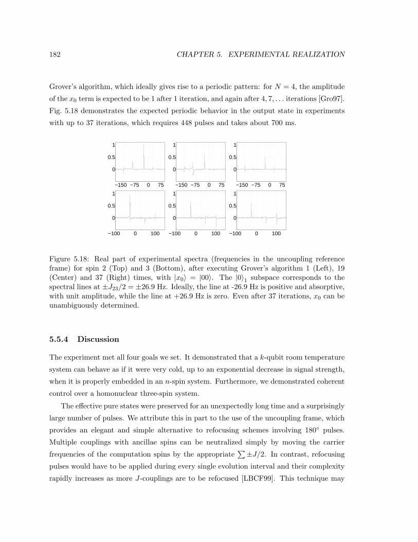
182 CHAPTER 5. EXPERIMENTAL REALIZATION
Grover’s algorithm, which ideally gives rise to a periodic pattern: for N = 4, the amplitude
of the x0 term is expected to be 1 after 1 iteration, and again after 4, 7, . . . iterations [Gro97].
Fig. 5.18 demonstrates the expected periodic behavior in the output state in experiments
with up to 37 iterations, which requires 448 pulses and takes about 700 ms.
−150 −75 0 75
0
0.5
1
−150 −75 0 75
0
0.5
1
−150 −75 0 75
0
0.5
1
−100 0 100
0
0.5
1
−100 0 100
0
0.5
1
−100 0 100
0
0.5
1
Figure 5.18: Real part of experimental spectra (frequencies in the uncoupling referenceframe) for spin 2 (Top) and 3 (Bottom), after executing Grover’s algorithm 1 (Left), 19(Center) and 37 (Right) times, with |x0〉 = |00〉. The |0〉1 subspace corresponds to thespectral lines at ±J23/2 = ±26.9 Hz. Ideally, the line at -26.9 Hz is positive and absorptive,with unit amplitude, while the line at +26.9 Hz is zero. Even after 37 iterations, x0 can beunambiguously determined.
5.5.4 Discussion
The experiment met all four goals we set. It demonstrated that a k-qubit room temperature
system can behave as if it were very cold, up to an exponential decrease in signal strength,
when it is properly embedded in an n-spin system. Furthermore, we demonstrated coherent
control over a homonuclear three-spin system.
The effective pure states were preserved for an unexpectedly long time and a surprisingly
large number of pulses. We attribute this in part to the use of the uncoupling frame, which
provides an elegant and simple alternative to refocusing schemes involving 180 pulses.
Multiple couplings with ancillae spins can be neutralized simply by moving the carrier
frequencies of the computation spins by the appropriate∑±J/2. In contrast, refocusing
pulses would have to be applied during every single evolution interval and their complexity
rapidly increases as more J-couplings are to be refocused [LBCF99]. This technique may
5.6. LIQUID CRYSTAL SOLUTIONS (2 SPINS) 183
find application in future experiments using logical labeling, as well as in quantum error
detection experiments [LVZ+99], where the computation must only proceed within the
subspace labeled error-free by the ancillae. However, refocusing pulses are still required
whenever a coupling must be removed over an entire system rather than in a subspace only.
In addition to decoherence, errors mainly arise from imperfections in the pulses and
coupled evolution during the 300 µs pulses (reduction of τ1 and τ2 partially compensated
for this effect). Spectra of the quality of Fig. 5.18 were obtained by choosing a particular
implementation of the composite z rotation in the phase flip step, such that the errors it
introduces partially cancel with the errors of the inversion step. For example, while Y XY ,
Y X Y, XY X and XY X are all mathematically equivalent, the errors may in practice add
up or cancel out with the errors from previous or subsequent pulse sequence segments.
Clearly, a general optimization procedure will be very helpful for designing effective pulse
sequences in future experiments involving more qubits.
5.6 Liquid crystal solutions (2 spins)
5.6.1 Problem description
The goal of this experiment [YSV+99]9 was to explore the use of liquid crystal solvents for
quantum computing. In principle, liquid crystals offer several advantages over liquids as
solvents for molecules used for NMR quantum computing. A liquid crystal solvent partly
orients the solute molecules (Fig. 5.19) and as a result, the dipolar coupling between nuclear
spins in molecules is not averaged out anymore as it is in isotropic solution. Liquid crystal
solvents therefore permit a significant increase in clock frequency, while short spin-lattice
relaxation times permit fast succession of experiments. Even more importantly, the clock
frequency may increase by more than the relaxation rates, so more operations may be
completed within the coherence time.
The coupling Hamiltonian for n spins in a molecule dissolved in a liquid crystal solvent
9Nino Yannoni proposed to use liquid crystal solvents instead of liquid solvents. He also selected asuitable liquid crystal solvent and prepared the sample. Mark Kubinec (at UC Berkeley) and I (at IBM)did experiments. The published data were taken at IBM. Mark Sherwood and Dolores Miller simulated thespectra and verified first-orderness. This work was done under the guidance of Ike Chuang.
184 CHAPTER 5. EXPERIMENTAL REALIZATION
!!!!!!!!!!!!
""""""""""""
Figure 5.19: Liquid crystals are a phase of matter whose order is intermediate betweenthat of a liquid and that of a crystal. The molecules are typically rod-shaped organicmoieties about 25 Angstroms in length and their ordering is a function of temperature.The liquid crystal shown here is in the nematic phase. The degree of orientational order ofthe constituent molecules decreases with decreasing temperature.
is
Hlc/~ = −n∑i
ω′i0 I
iz+
n∑i<j
Jij(IixIjx+IiyI
jy +IizI
jz )+
n∑i<j
Dij
[2IizI
jz −
12
(IixIjx + IiyI
jy)]. (5.6)
A dipolar term, which was absent from the coupling Hamiltonian in liquid solution (Eq. 4.5)
now appears because the molecules are partially oriented. Also the resonance frequency ω′i0includes the effects of molecular orientation and chemical shift anisotropy [EL75]. The
dipolar coupling strength D, which also depends on the orientation, is typically 100 Hz to
10 kHz.
Unfortunately, the pulse sequences used for NMR quantum computing in isotropic liq-
uids can not be applied if the Hamiltonian takes the form of Eq. 5.6. However, for an n-spin
system with first order spectra, Eq. 5.6 becomes [SEP67]
H lc = −n∑i=1
~ω′i0 I
iz + ~
n∑i<j
2π(Jij + 2Dij)IizIjz , (5.7)
This Hamiltonian has the same form as the Hamiltonian of Eq. 4.5, so the pulse sequences
that have been used successfully for NMR quantum computing in isotropic solution can
now be applied directly to liquid crystal solutions, permitting computations with fclock =
2|(J + 2D)| Hz, a frequency that can be much higher than 2|J |.

5.6. LIQUID CRYSTAL SOLUTIONS (2 SPINS) 185
5.6.2 Experimental approach and results
We chose 13C-labeled chloroform (CHCl3) as the quantum computer molecule. This is the
molecule we had used successfully in the first quantum computing experiments. The liquid
crystal we selected was ZLI-167 (EMI Industries, Hawthorne, NY).
Table 5.1 shows the 13C - 1H coupling strength, the spin-lattice relaxation time (T1) and
the spin-spin relaxation time (T2) for 13C and 1H in chloroform (13CHCl3) in liquid crystal
solution and for comparison also in isotropic solution, both at ambient temperature.
solvent J J + 2D T1 (13C) T1 (1H) T2 (13C) T2 (1H)acetone-d6 215 25 19 0.3 7ZLI-1167 1706 2 1.4 0.2 0.7
Table 5.1: 13C-1H spin couplings [Hz] and relaxation times [s] for 13C1HCl3 in isotropic(deuterated acetone) and liquid crystal (ZLI-1167) solution.
In order to show that quantum computations can be done successfully using liquid-
crystal solution NMR, we have implemented the Grover search algorithm for two qubits
using 13CHCl3 dissolved in ZLI-1167. The carbon and proton spins were first prepared in an
effective pure state created by temporal labeling (via cyclic permutations, see section 4.4.4)
followed by the Grover protocol used in the logical labeling experiment of section 5.5.
The prediction is that the algorithm will put the spins in the state |x0〉. The 13C and 1H
readout spectra for the four possible x0 are shown in Fig. 5.20. As predicted for two spins
in an effective pure state, the value of x0 is clearly indicated by the amplitude and phase of
the two resonance lines in the 13C and 1H spectra. Measurement of the deviation density
matrix using quantum state tomography confirms that the output states are as theoretically
predicted, as illustrated in Fig. 5.21 for x0 = 11.

186 CHAPTER 5. EXPERIMENTAL REALIZATION
−1
0
1
−1
0
1
−1
0
1
−1
0
1
−1
0
1
−1
0
1
−1 0 1−1
0
1
[kHz]−1 0 1
−1
0
1
[kHz]
Figure 5.20: Spectral readout of the results of the 2-qubit Grover search using 13C1HCl3 ina liquid crystal solvent showing absorption and emission peaks which clearly indicate thevalue of x0 (00, 01, 10, and 11, from top to bottom). The real part of the 1H (left) and 13C(right) spectra are shown, with frequencies relative to ωH0 /2π and ωC0 ). The vertical scaleis arbitrary.
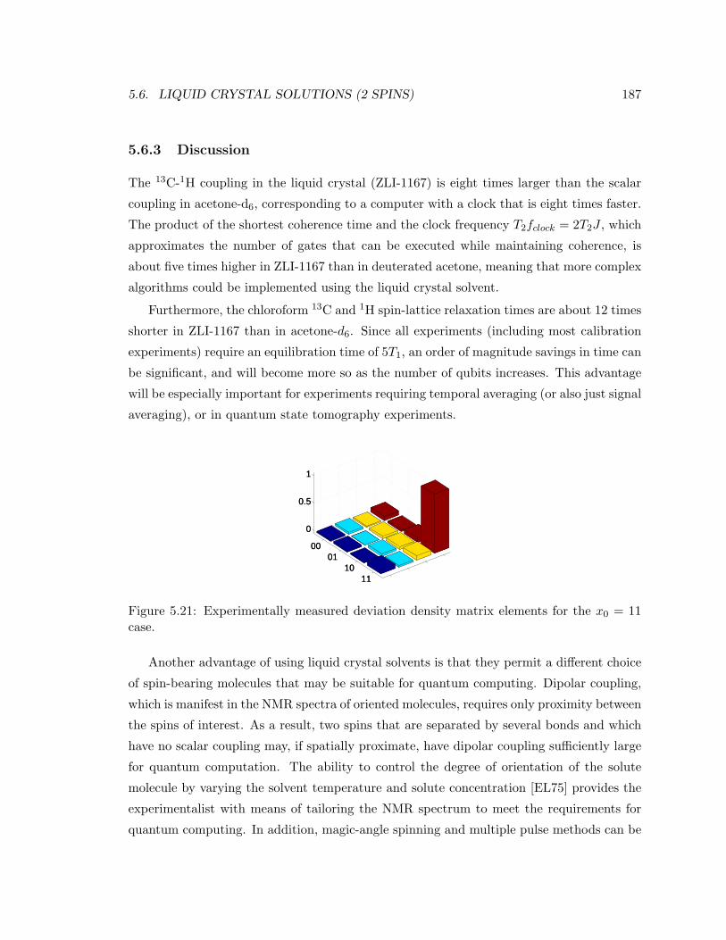
5.6. LIQUID CRYSTAL SOLUTIONS (2 SPINS) 187
5.6.3 Discussion
The 13C-1H coupling in the liquid crystal (ZLI-1167) is eight times larger than the scalar
coupling in acetone-d6, corresponding to a computer with a clock that is eight times faster.
The product of the shortest coherence time and the clock frequency T2fclock = 2T2J , which
approximates the number of gates that can be executed while maintaining coherence, is
about five times higher in ZLI-1167 than in deuterated acetone, meaning that more complex
algorithms could be implemented using the liquid crystal solvent.
Furthermore, the chloroform 13C and 1H spin-lattice relaxation times are about 12 times
shorter in ZLI-1167 than in acetone-d6. Since all experiments (including most calibration
experiments) require an equilibration time of 5T1, an order of magnitude savings in time can
be significant, and will become more so as the number of qubits increases. This advantage
will be especially important for experiments requiring temporal averaging (or also just signal
averaging), or in quantum state tomography experiments.
0001
1011
0
0.5
1
Figure 5.21: Experimentally measured deviation density matrix elements for the x0 = 11case.
Another advantage of using liquid crystal solvents is that they permit a different choice
of spin-bearing molecules that may be suitable for quantum computing. Dipolar coupling,
which is manifest in the NMR spectra of oriented molecules, requires only proximity between
the spins of interest. As a result, two spins that are separated by several bonds and which
have no scalar coupling may, if spatially proximate, have dipolar coupling sufficiently large
for quantum computation. The ability to control the degree of orientation of the solute
molecule by varying the solvent temperature and solute concentration [EL75] provides the
experimentalist with means of tailoring the NMR spectrum to meet the requirements for
quantum computing. In addition, magic-angle spinning and multiple pulse methods can be

188 CHAPTER 5. EXPERIMENTAL REALIZATION
used to preferentially scale the dipolar splitting in the spectrum of a liquid-crystal-oriented
molecule to convert it to first order [OOC+91].
Complications do arise with the use of liquid crystal solvents: (1) the NMR lines of small
molecules dissolved in liquid crystal solvents are susceptible to a broadening mechanism not
found in isotropic solution, most likely due to variations in the degree of orientation caused
by thermal gradients in the sample. Nonetheless, resonance line widths < 2 Hz (13C) and
< 3 Hz (1H) were obtained for 13C1HCl3 in ZLI-1167; (2) the large dipolar couplings may
cause unwanted evolution of the spins during the RF pulses, especially in homonuclear spin
systems.
We have not used liquid crystal solvents in any of the later experiments. However, due
to their many advantages and only moderate disadvantages, we believe it is worth revisiting
this possibility in the context of larger spin systems.
5.7 Cancellation and prevention of systematic errors (3 spins)
5.7.1 Problem description
In this experiment [VSS+00]10 we studied the effect of systematic errors in the one-qubit
gates. Aside from the well-understood scaling limitations due to the use of a high-temperature
(almost random) system instead of a low-temperature (low entropy) polarized spin sys-
tem (section 4.4), such errors represent an important limitation in using nuclear spins in
molecules to implement larger quantum algorithms.
Single-qubit gates are implemented by applying RF pulses of precise duration and phase,
but which in practice greatly vary in strength over the sample volume, causing the gate
fidelity [SN96] to be less than 95% (section 5.1). Producing a homogeneous RF field is
difficult because of the sample geometry and the necessity of keeping the B1 field transverse
to the B0 field. If such systematic errors simply accumulated, these observations would
imply that for a success rate of only 1%, fewer than 90 gates (0.9590 ≈ 0.01) applied to any
one spin could ever be cascaded in these systems.
10I worked out the theory and many of the pulse sequence simplification ideas, along with Matthias Steffenand Ike Chuang. The simplified temporal averaging scheme is due to Ike. The experiment and data analysiswas done by myself and Matthias. The molecule was synthesized by Greg Breyta, and proposed by NinoYannoni and Mark Sherwood, who also gave advice on NMR techniques.

5.7. CANCELLATION AND PREVENTION OF SYSTEMATIC ERRORS (3 SPINS)189
One technique which has been proposed for controlling errors in quantum gates is quan-
tum error correction (section 2.4), but this is associated with a large overhead. The prin-
ciple attribute of quantum error correction techniques is their ability to correct completely
random errors which originate from fundamentally irreversible decoherence phenomena; in
principle, systematic errors, which are inherently reversible — at least on an appropriate
time scale — should be much easier to control, given knowledge about their origin.
We tested the extent to which systematic errors can (1) be avoided by simplifying the
pulse sequences and (2) be made to cancel out in practice. The concrete experiment for
this test consisted of repeated executions of the two main steps in Grover’s algorithm (the
oracle call and the inversion about the average described in section 2.3.2) for three spins.
The three-qubit Grover algorithm can find a “marked” element x0 among N = 8 possible
values of x in only two oracle queries (evaluations of f(x)), whereas a classical search needs
4.375 attempts on average to find x0. The oracle call requires one Toffoli gate plus
several one-qubit gates, and so thus the inversion about the average. The amplitude of |x0〉is predicted to reach a first maximum after two iterations, and oscillates as the number of
iterations increases.
5.7.2 Experimental approach
The first method we developed to reduce the number of one- and two-spin gates needed to
implement arbitrary unitary operations was the general pulse simplification methodology
of section 4.8. As a result, the pulse sequence for each Toffoli gate used in the algorithm
was reduced from 70.5 90 pulses and 8 evolutions of 1/2J (if only cnot’s and 1-qubit
gates would have been used to implement the controlled-V ’s, as in the standard methods
of [BBC+95]) to 19 pulses, 2 evolutions of 1/2J and 3 of 1/4J .
The second method to reduce the complexity concerns the initialization of the qubits
to an effective ground state. We generalized the temporal averaging procedure from a
scheme based on cyclic permutations to a scheme based on arbitrary linearly independent
experiments (section 4.4). Whereas cyclic permutations would require seven experiments
with very complex state preparation sequences, all the data shown here were obtained using
just three experiments with much simpler preparation sequences. The expected variance of
the 2n − 1 populations obtained with this state preparation procedure amounts to only 7%
of their average value.
The actual pulse sequences used in the experiment are collected in Appendix B.

190 CHAPTER 5. EXPERIMENTAL REALIZATION
5.7.3 Experimental Results
We selected 13C-labeled CHFBr211 for our experiments. The 1H, 19F and 13C spins served
as the quantum bits. The coupling constants in this heteronuclear spin system are JHC =
224 Hz, JHF = 50 Hz and JFC = −311 Hz. As always, the scalar interaction with the Br
nuclei is averaged out and only contributes to decoherence.
In order to read out the final state of the three spins, we used the extra information
given by the multiple lines in the spectrum of each spin. Given that all three spins are in
an effective pure energy eigenstate and that they are all mutually coupled, each spectrum
contains only a single line, the frequency of which, combined with the knowledge of the Jij ,
reveals the state of the remaining spins. The inset of Fig. 5.22 (a) gives the experimentally
measured 13C output spectrum after two Grover iterations. Fig. 5.22 (a) also gives the
complete output deviation density matrix.
000
111
00.10.20.30.4
[arb
itrar
y un
its]
000
111
00.020.040.06
[arb
itrar
y un
its]
Figure 5.22: (Top) Experimental deviation density matrices ρexp for |x0〉 = |1〉|0〉|1〉, shownin magnitude with the sign of the real part (all imaginary components were small), after (a)2 and (b) 28 Grover iterations. (Bottom) The corresponding 13C spectra (13C was the leastsignificant qubit). The receiver phase and read-out pulse are set such that the spectrum beabsorptive and positive for a spin in |0〉.
The agreement between experimental results and theoretical predictions is good, con-
sidering that about 100 pulses were used and that the systematic error rate exceeds 5% per
RF pulse (the measured signal loss due to RF field inhomogeneity after applying Xi). This11Synthesized by heating a mixture of 13CHBr3 (2.25 g, CIL) and HgF2 (2.8 g, Aldrich) in increments
(5C for 15 min) from 70C to 85C in a Kugelrohr apparatus and condensing the product into a cooledbulb. This material was re-distilled bulb-to-bulb at 65C to give 750 mg (99 % purity) of 13CHFBr2, whichwas dissolved in d6-acetone.

5.7. CANCELLATION AND PREVENTION OF SYSTEMATIC ERRORS (3 SPINS)191
suggests that the systematic errors cancel each other out to some degree. We examined this
in more detail in a series of experiments with increasingly longer pulse sequences executing
up to 28 Grover iterations (Fig. 5.23).
0 10 20 30−0.2
0
0.2
0.4
0.6
0.8
0 10 20 300
0.2
0.4
0.6
0.8
1
c=1 c=1/lossfit
Figure 5.23: (a) Experimental (error bars) and ideal (circles) amplitude of dx0 , with fits(dotted) to guide the eye. Dashed line: the signal decay for 13C due to intrinsic phaserandomization or decoherence (for 13C, T2 ≈ 0.65 s). Solid line: the signal strength retainedafter applying a continuous RF pulse of the same cumulative duration per Grover iterationas the pulses in the Grover sequence (averaged over the three spins; measured up to 4iterations and then extrapolated). (b) The relative error εr.
5.7.4 Discussion
Fig. 5.23 (a) shows that the diagonal entry dx0 of ρexp oscillates as predicted but the oscil-
lation is damped as a result of errors, with a time constant Td of 12.8 iterations. However,
Td would have been smaller than 1.5 if the errors due to just the RF field inhomogeneity
were cumulative (Fig. 5.23 (a), solid line). Remarkably, after a considerable initial loss, dx0
decays at a rate close to the 13C T2 decay rate (dashed line), which can be regarded as a
lower bound on the overall error rate.
A more complete measure to quantify the error and benchmark results is the relative
error εr =‖ cρexp−ρth ‖2 / ‖ ρth ‖2, where ρexp and ρth are the experimental and theoretical
(traceless) deviation density matrices. Comparison of εr with c = 1 and c equal to the inverse
of the signal loss (Fig. 5.23 (b)) reveals that signal loss dominates over other types of error.
Furthermore, the small values of εr with c > 1 suggest that |x0〉 can be unambiguously
identified, even after almost 1350 pulses. This is confirmed by the density matrix measured
192 CHAPTER 5. EXPERIMENTAL REALIZATION
after 28 iterations, which has a surprisingly good signature (Fig. 5.22 (b)). Given the
error of > 5% per single 90 rotation, all these observations demonstrate that substantial
cancellation of errors took place in our experiments.
The error cancellation achieved was partly due to a judicious choice of the phases of
the refocusing pulses, but a detailed mathematical description in terms of error operators is
needed to fully exploit this effect in arbitrary pulse sequences. This difficult undertaking is
made worthwhile by our observations. This conclusion is strengthened by a similar observa-
tion in the experiment of section 5.5. Also, we believe that error cancellation behavior is not
just a property of the Grover iterations, because we found experimentally that the choice
of implementation of the building blocks dramatically affects the cancellation effectiveness.
In summary, more than 280 two-qubit quantum gates involving 1350 RF pulses were
successfully cascaded, which far exceeds not only the number of gates used in all previous
NMR quantum computing experiments but also the limitation of 90 pulses, imposed by cu-
mulative systematic errors. Whereas the cancellation of systematic errors makes it possible
to perform such a surprisingly large number of operations, the methods for simplifying pulse
sequences reduce the number of operations needed to implement a given quantum circuit.
This combination permitted the observation of 28 full cycles of the Grover algorithm with
3 spins, and suggests that many other interesting quantum computing experiments may be
within reach.
5.8 Efficient cooling (3 spins)
5.8.1 Problem description
The goal of this experiment [CVS01]12 was to cool down the spin temperature of one out of
three spins using the Schulman-Vazirani scheme for efficient cooling [SV99]. A secondary
goal was to draw the attention of the quantum computing community to the Schulman-
Vazirani algorithm.
The ideas underlying Schulman-Vazirani cooling have been introduced in section 3.1.3.
The quantum circuit which summarizes the steps in the Schulman-Vazirani boosting pro-
cedure, was described in section 4.4.6, Fig. 5.24. We include it here again for convenience.
12I devised this experiment. Darrick Chang, a summer student, worked out the pulse sequences and tookthe data under my guidance, and with the help of Matthias Steffen.

5.8. EFFICIENT COOLING (3 SPINS) 193
1
2
3
Figure 5.24: A quantum circuit that implements the Schulman-Vazirani boosting procedurefor cooling one out of three qubits.
While it is common in NMR to enhance the polarization of a low-γ nucleus by polar-
ization transfer from a high-γ nucleus [EBW87, Fre97], in this experiment the goal was to
enhance the polarization of one out of three equally polarized spins. Any polarization gain
is thus exclusively the result of bootstrapping using the Schulman-Vazirani cooling scheme.
In this case, the theoretical maximum achievable polarization enhancement is by a factor
of 3/2; this is equivalent to lowering the spin temperature of that spin by the same factor.
5.8.2 Experimental procedure and results
A 2 mol % solution of C2F3Br in deuterated acetone provided three spins with equal polar-
izations. We chose this particular molecule for its remarkable spectral properties (we had
successfully used it in the logical labeling experiment of section 5.5): strong chemical shifts
(0, 28.2, and 48.1 ppm, arbitrarily referenced) and large scalar couplings (Jab = −122.1 Hz,
Jac = 75.0 Hz, and Jbc = 53.8 Hz) combined with long relaxation times (T2’s ≈ 4-8 s). The
experiments were conducted at 30.0C.
The quantum circuit of Fig. 5.24 results in the unitary operation (with qubit 1 the most
significant qubit)
U =
0 1 0 0 0 0 0 0
1 0 0 0 0 0 0 0
0 0 1 0 0 0 0 0
0 0 0 0 1 0 0 0
0 0 0 0 0 1 0 0
0 0 0 1 0 0 0 0
0 0 0 0 0 0 1 0
0 0 0 0 0 0 0 1
, (5.8)
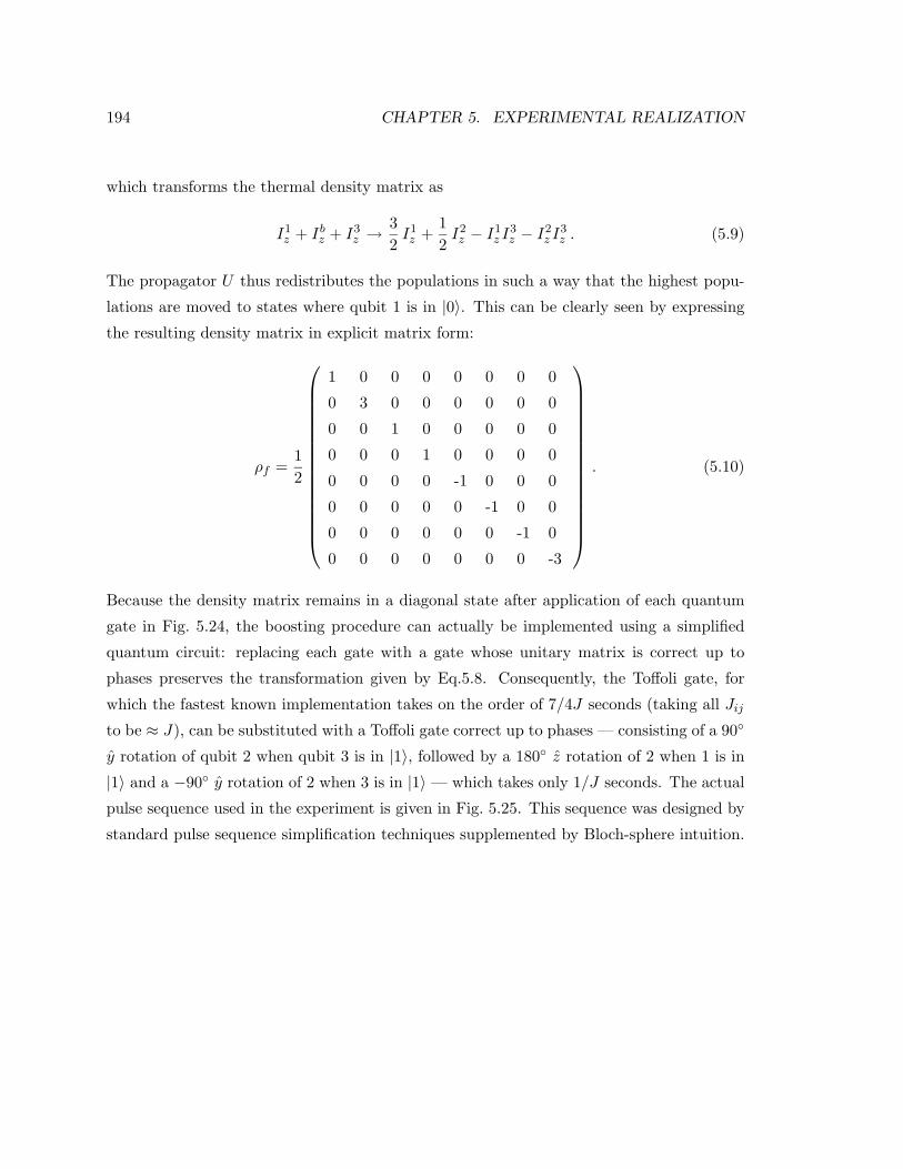
194 CHAPTER 5. EXPERIMENTAL REALIZATION
which transforms the thermal density matrix as
I1z + Ibz + I3
z →32I1z +
12I2z − I1
z I3z − I2
z I3z . (5.9)
The propagator U thus redistributes the populations in such a way that the highest popu-
lations are moved to states where qubit 1 is in |0〉. This can be clearly seen by expressing
the resulting density matrix in explicit matrix form:
ρf =12
1 0 0 0 0 0 0 0
0 3 0 0 0 0 0 0
0 0 1 0 0 0 0 0
0 0 0 1 0 0 0 0
0 0 0 0 -1 0 0 0
0 0 0 0 0 -1 0 0
0 0 0 0 0 0 -1 0
0 0 0 0 0 0 0 -3
. (5.10)
Because the density matrix remains in a diagonal state after application of each quantum
gate in Fig. 5.24, the boosting procedure can actually be implemented using a simplified
quantum circuit: replacing each gate with a gate whose unitary matrix is correct up to
phases preserves the transformation given by Eq.5.8. Consequently, the Toffoli gate, for
which the fastest known implementation takes on the order of 7/4J seconds (taking all Jijto be ≈ J), can be substituted with a Toffoli gate correct up to phases — consisting of a 90
y rotation of qubit 2 when qubit 3 is in |1〉, followed by a 180 z rotation of 2 when 1 is in
|1〉 and a −90 y rotation of 2 when 3 is in |1〉— which takes only 1/J seconds. The actual
pulse sequence used in the experiment is given in Fig. 5.25. This sequence was designed by
standard pulse sequence simplification techniques supplemented by Bloch-sphere intuition.

5.8. EFFICIENT COOLING (3 SPINS) 195
The resulting unitary operator is
U =
0 1 0 0 0 0 0 0
1 0 0 0 0 0 0 0
0 0 -1 0 0 0 0 0
0 0 0 0 -1 0 0 0
0 0 0 0 0 1 0 0
0 0 0 -1 0 0 0 0
0 0 0 0 0 0 1 0
0 0 0 0 0 0 0 1
. (5.11)
Figure 5.25: Pulse sequence used to implement the boosting procedure. This pulse sequenceis designed for molecules with Jab < 0 and Jac, Jbc > 0.
All pulses were spin-selective, and varied in duration from 1 to 3 ms. Hermite 180
and av90 shaped pulses were employed for 180 and 90 rotations respectively, in order to
minimize the effect of the J couplings between the selected and non-selected spins during
the pulses. Couplings between the unselected spins are irrelevant whenever those spins are
along ±z, as is the case here.
Bloch-Siegert shifts (sections 4.2.4 and 4.2.5) were accounted for in the pulse sequence
out of necessity: they resulted in an extra phase acquired by the non-selected spins in their
respective on-resonance reference frames, in some cases by more than 90 per pulse, while
even phase shifts on the order of 5 are unacceptable. Bloch-Siegert corrections and other
z rotations were implicitly performed by changing the phase of subsequent RF pulses. The
duration of the pulse sequence of Fig. 5.25 is about 70 ms.

196 CHAPTER 5. EXPERIMENTAL REALIZATION
5.8.3 Experimental results
The theoretical predictions for the spectrum of each spin after the boosting procedure can
be derived most easily from Eq. 5.10, taking into account the sign and magnitude of the J-
couplings. After a readout pulse on spin 1, the four spectral lines in the spectrum of 1 should
ideally have normalized amplitudes 1 : 2 : 1 : 2, compared to 1 : 1 : 1 : 1 for the thermal
equilibrium spectrum (for spins 2 and 3, the boosting procedure ideally results in normalized
amplitudes of 0 : 1 : 0 : 1 and −1 : 0 : 0 : 1, respectively). So the prediction is that the
boosting procedure increases the signal of spin 1 averaged over the four spectral lines by a
factor of 3/2, equal to the bound for polarization enhancement established in section 4.4.6.
The experimentally measured spectra before and after the boosting procedure are shown in
Fig. 5.26. The operation of the boosting procedure was further validated by measuring the
full three-spin deviation density matrix, shown in Fig. 5.27.
−100 0 100−1
0
1
2
−100 0 100−1
0
1
2
−100 0 100−1
0
1
2
−100 0 100−1
0
1
2
−100 0 100−1
0
1
2
−100 0 100−1
0
1
2
Figure 5.26: Experimentally measured spectra of spin 1 (Left), spin 2 (Center) and spin3 (Right), after a readout pulse on the corresponding spin, for the spin system in thermalequilibrium (Top) and after applying the boosting procedure (Bottom). The real part ofthe spectra is shown, and the spectra were rescaled in order to obtain unit amplitude for thethermal equilibrium spectra. Frequencies are in Hz with respect to the Larmour frequencyof the respective spins.
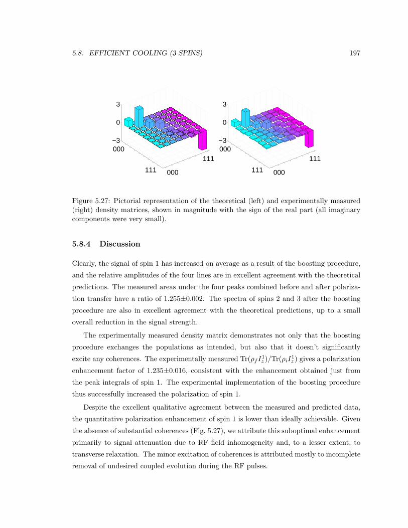
5.8. EFFICIENT COOLING (3 SPINS) 197
000
111000
111
−3
0
3
000
111000
111
−3
0
3
Figure 5.27: Pictorial representation of the theoretical (left) and experimentally measured(right) density matrices, shown in magnitude with the sign of the real part (all imaginarycomponents were very small).
5.8.4 Discussion
Clearly, the signal of spin 1 has increased on average as a result of the boosting procedure,
and the relative amplitudes of the four lines are in excellent agreement with the theoretical
predictions. The measured areas under the four peaks combined before and after polariza-
tion transfer have a ratio of 1.255±0.002. The spectra of spins 2 and 3 after the boosting
procedure are also in excellent agreement with the theoretical predictions, up to a small
overall reduction in the signal strength.
The experimentally measured density matrix demonstrates not only that the boosting
procedure exchanges the populations as intended, but also that it doesn’t significantly
excite any coherences. The experimentally measured Tr(ρfI1z )/Tr(ρiI1
z ) gives a polarization
enhancement factor of 1.235±0.016, consistent with the enhancement obtained just from
the peak integrals of spin 1. The experimental implementation of the boosting procedure
thus successfully increased the polarization of spin 1.
Despite the excellent qualitative agreement between the measured and predicted data,
the quantitative polarization enhancement of spin 1 is lower than ideally achievable. Given
the absence of substantial coherences (Fig. 5.27), we attribute this suboptimal enhancement
primarily to signal attenuation due to RF field inhomogeneity and, to a lesser extent, to
transverse relaxation. The minor excitation of coherences is attributed mostly to incomplete
removal of undesired coupled evolution during the RF pulses.
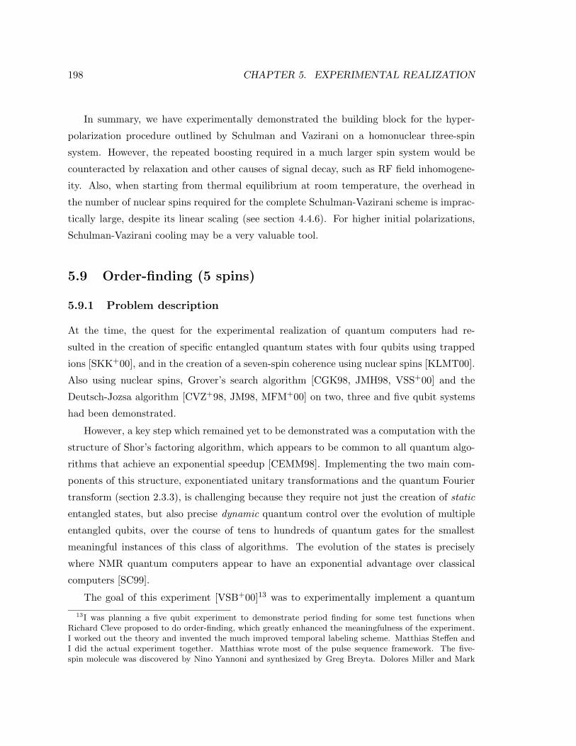
198 CHAPTER 5. EXPERIMENTAL REALIZATION
In summary, we have experimentally demonstrated the building block for the hyper-
polarization procedure outlined by Schulman and Vazirani on a homonuclear three-spin
system. However, the repeated boosting required in a much larger spin system would be
counteracted by relaxation and other causes of signal decay, such as RF field inhomogene-
ity. Also, when starting from thermal equilibrium at room temperature, the overhead in
the number of nuclear spins required for the complete Schulman-Vazirani scheme is imprac-
tically large, despite its linear scaling (see section 4.4.6). For higher initial polarizations,
Schulman-Vazirani cooling may be a very valuable tool.
5.9 Order-finding (5 spins)
5.9.1 Problem description
At the time, the quest for the experimental realization of quantum computers had re-
sulted in the creation of specific entangled quantum states with four qubits using trapped
ions [SKK+00], and in the creation of a seven-spin coherence using nuclear spins [KLMT00].
Also using nuclear spins, Grover’s search algorithm [CGK98, JMH98, VSS+00] and the
Deutsch-Jozsa algorithm [CVZ+98, JM98, MFM+00] on two, three and five qubit systems
had been demonstrated.
However, a key step which remained yet to be demonstrated was a computation with the
structure of Shor’s factoring algorithm, which appears to be common to all quantum algo-
rithms that achieve an exponential speedup [CEMM98]. Implementing the two main com-
ponents of this structure, exponentiated unitary transformations and the quantum Fourier
transform (section 2.3.3), is challenging because they require not just the creation of static
entangled states, but also precise dynamic quantum control over the evolution of multiple
entangled qubits, over the course of tens to hundreds of quantum gates for the smallest
meaningful instances of this class of algorithms. The evolution of the states is precisely
where NMR quantum computers appear to have an exponential advantage over classical
computers [SC99].
The goal of this experiment [VSB+00]13 was to experimentally implement a quantum
13I was planning a five qubit experiment to demonstrate period finding for some test functions whenRichard Cleve proposed to do order-finding, which greatly enhanced the meaningfulness of the experiment.I worked out the theory and invented the much improved temporal labeling scheme. Matthias Steffen andI did the actual experiment together. Matthias wrote most of the pulse sequence framework. The five-spin molecule was discovered by Nino Yannoni and synthesized by Greg Breyta. Dolores Miller and Mark

5.9. ORDER-FINDING (5 SPINS) 199
algorithm for finding the order of a permutation (section 2.3.3); its structure is the same as
for Shor’s factoring algorithm and it scales exponentially faster than any classical algorithm
for the problem.
Specifically, we set out to implement the smallest instance of order-finding for which
quantum computers outperform classical computers: the case of permutations π on four
elements (M = 4), using a total of five qubits (m = 2 and n = 3).
It can be proven that in this case the best classical algorithm needs two queries of
the oracle to determine r with certainty, and that using only one query of the oracle, the
probability of finding r using a classical algorithm can be no more than 1/2. One optimal
classical strategy is to first ask the oracle for the value of π3(y): when the result is y, r
must be 1 or 3; otherwise r must be 2 or 4. In either case, the actual order can be guessed
only with probability 1/2.
In contrast, the probability of success is ∼ 0.55 after only one oracle-query using the
quantum circuit of Fig. 2.13 on a single quantum computer: depending on the measurement
outcome after running the algorithm, we can make a probabilistic guess r′ as shown in
Fig. 5.28. The probability of success Pr[r′ = r] is independent of the distribution of r or π.
Figure 5.28: (Left) The probabilities that the measurement result m is 0, 1, . . . , or 7, givenr (for an ideal single quantum computer). (Right) The optimal probabilities with which tomake a guess r′ for r, given m.
Note that since an ensemble of ∼ 1018 quantum computers contribute to the signal in
our experiment, the order will follow from the output data with virtual certainty.
5.9.2 Experimental approach
We custom synthesized a molecule [GMS68] containing five fluorine nuclear spins which
served as the qubits. The molecule as well as the chemical shifts and J-coupling constants
are shown in Fig. 5.29. The linewidths of the NMR transitions were ∼ 1 Hz, so the T ∗2
Sherwood did spectral simulations of the molecule. All this work was done under the guidance of Ike Chuang.
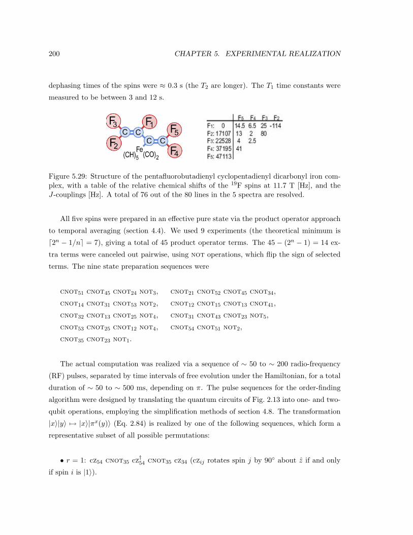
200 CHAPTER 5. EXPERIMENTAL REALIZATION
dephasing times of the spins were ≈ 0.3 s (the T2 are longer). The T1 time constants were
measured to be between 3 and 12 s.
Figure 5.29: Structure of the pentafluorobutadienyl cyclopentadienyl dicarbonyl iron com-plex, with a table of the relative chemical shifts of the 19F spins at 11.7 T [Hz], and theJ-couplings [Hz]. A total of 76 out of the 80 lines in the 5 spectra are resolved.
All five spins were prepared in an effective pure state via the product operator approach
to temporal averaging (section 4.4). We used 9 experiments (the theoretical minimum is
d2n − 1/ne = 7), giving a total of 45 product operator terms. The 45 − (2n − 1) = 14 ex-
tra terms were canceled out pairwise, using not operations, which flip the sign of selected
terms. The nine state preparation sequences were
cnot51 cnot45 cnot24 not3, cnot21 cnot52 cnot45 cnot34,
cnot14 cnot31 cnot53 not2, cnot12 cnot15 cnot13 cnot41,
cnot32 cnot13 cnot25 not4, cnot31 cnot43 cnot23 not5,
cnot53 cnot25 cnot12 not4, cnot54 cnot51 not2,
cnot35 cnot23 not1.
The actual computation was realized via a sequence of ∼ 50 to ∼ 200 radio-frequency
(RF) pulses, separated by time intervals of free evolution under the Hamiltonian, for a total
duration of ∼ 50 to ∼ 500 ms, depending on π. The pulse sequences for the order-finding
algorithm were designed by translating the quantum circuits of Fig. 2.13 into one- and two-
qubit operations, employing the simplification methods of section 4.8. The transformation
|x〉|y〉 7→ |x〉|πx(y)〉 (Eq. 2.84) is realized by one of the following sequences, which form a
representative subset of all possible permutations:
• r = 1: cz54 cnot35 cz†54 cnot35 cz34 (czij rotates spin j by 90 about z if and only
if spin i is |1〉).

5.9. ORDER-FINDING (5 SPINS) 201
• r = 2: cnot35.
• r = 3: cnot32 cnot25 cnot32 cnot21 cz14 cnot51 cz†14 cnot51 cz54 cnot21 cz15
cnot41 cz†15 cnot41 cz45. (this sequence does the transformation πx(y) for y = 2 only;
sequences for r = 3 that would work for any y are prohibitively long).
• r = 4: cnot24 cz34 cz54 cnot35 cz54.
Each transformation was tested independently to confirm its proper operation. All pulse
sequences were implemented on the four-channel spectrometer described in section 5.1, and
using the methods of section 4.2 to serve two qubits with one channel. The frequency of
one channel was set at (ω2 +ω3)/2, and the other three channels were set on the resonance
of spins 1, 4 and 5. The chemical shift evolutions of spins 2 and 3 were calculated with
the help of a time-counter, which kept track of the time elapsed from the start of the
pulse sequence. On-resonance excitation of spins 2 and 3 was achieved using phase-ramping
techniques. All pulses were spin-selective and Hermite shaped. Rotations about the z-axis
were implemented by adjusting the phases of the subsequent pulses. Unintended phase
shifts of spins i during a pulse on spin j 6= i were calculated and accounted for by adjusting
the phase of subsequent pulses. During simultaneous pulses, the effect of these phase shifts
was largely removed by shifting the frequency of the pulses via phase-ramping, in such a
way that they track the shifting spin frequencies and thereby greatly improve the accuracy
of the simultaneous rotations of two or more spins.
Upon completion of the pulse sequence, the states of the three spins in the first register
were measured and the order r was determined from the read-out. Since an ensemble of
quantum computers rather than a single quantum computer was used, the measurement
gives the bitwise average values of mi (i = 1, 2, 3), instead of a sample of m = m1m2m3
with probabilities given in Fig. 5.28 14. Formally, measurement of spin i returns Oi =
1 − 2〈mi〉 = 2 Tr(ρIzi), where ρ is the final density operator of the system. The Oi are
obtained experimentally from integrating the peak areas in the spectrum of the magnetic
signal of spin i after a 90 read-out pulse on spin i, phased such that positive spectral lines
correspond to positive Oi. The theoretically predicted values of Oi (i = 1, 2, 3) for each
value of r follow directly from the probabilities for m in Fig. 5.28. For reference, we also
include the values of O4 and O5 (for y = 0; if y 6= 0, O4 and O5 can be negative): for the case
14It is not clear that the bitwise average outputs of the QFT suffice to determine r for permutations onarbitrary n. Instead, the continued fraction expansion can be ran on the quantum computer to compute r.
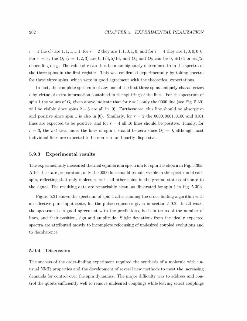
202 CHAPTER 5. EXPERIMENTAL REALIZATION
r = 1 the Oi are 1, 1, 1, 1, 1; for r = 2 they are 1, 1, 0, 1, 0; and for r = 4 they are 1, 0, 0, 0, 0.
For r = 3, the Oi (i = 1, 2, 3) are 0, 1/4, 5/16, and O4 and O5 can be 0, ±1/4 or ±1/2,
depending on y. The value of r can thus be unambiguously determined from the spectra of
the three spins in the first register. This was confirmed experimentally by taking spectra
for these three spins, which were in good agreement with the theoretical expectations.
In fact, the complete spectrum of any one of the first three spins uniquely characterizes
r by virtue of extra information contained in the splitting of the lines. For the spectrum of
spin 1 the values of Oi given above indicate that for r = 1, only the 0000 line (see Fig. 5.30)
will be visible since spins 2 − 5 are all in |0〉. Furthermore, this line should be absorptive
and positive since spin 1 is also in |0〉. Similarly, for r = 2 the 0000, 0001, 0100 and 0101
lines are expected to be positive, and for r = 4 all 16 lines should be positive. Finally, for
r = 3, the net area under the lines of spin 1 should be zero since O1 = 0, although most
individual lines are expected to be non-zero and partly dispersive.
5.9.3 Experimental results
The experimentally measured thermal equilibrium spectrum for spin 1 is shown in Fig. 5.30a.
After the state preparation, only the 0000 line should remain visible in the spectrum of each
spin, reflecting that only molecules with all other spins in the ground state contribute to
the signal. The resulting data are remarkably clean, as illustrated for spin 1 in Fig. 5.30b.
Figure 5.31 shows the spectrum of spin 1 after running the order-finding algorithm with
an effective pure input state, for the pulse sequences given in section 5.9.2. In all cases,
the spectrum is in good agreement with the predictions, both in terms of the number of
lines, and their position, sign and amplitude. Slight deviations from the ideally expected
spectra are attributed mostly to incomplete refocusing of undesired coupled evolutions and
to decoherence.
5.9.4 Discussion
The success of the order-finding experiment required the synthesis of a molecule with un-
usual NMR properties and the development of several new methods to meet the increasing
demands for control over the spin dynamics. The major difficulty was to address and con-
trol the qubits sufficiently well to remove undesired couplings while leaving select couplings

5.10. SHOR’S FACTORING ALGORITHM (7 SPINS) 203
−50 0 500
2
4
6
8
10
0000
0010
0001
0011
0100
0110
0101
0111
1111
1101
1110
1100
1011
1001
1010
1000
a
−50 0 50
0
40
80
− − − − − − − −−−−−−−−−b
Figure 5.30: (a) The spectrum of spin 1 in thermal equilibrium. Taking into account thesign and magnitude of the J1,j , the 16 lines in the spectrum of spin 1 can be labeled asshown. (b) The same spectrum when the spins are in an effective pure state. Only theline labeled 0000 is present. All spectra shown here and in Fig. 5.31 display the real partof the spectrum in the same arbitrary units, and were obtained without phase cycling orsignal-averaging (except for Fig. 5.31 c, where 16 identical scans were averaged). A 0.1 Hzfilter was applied. Frequencies are in units of Hz with respect to ω1/2π.
active — much of the more advanced techniques for single-qubit rotations presented in sec-
tion 4.2 were developed for this experiment. Furthermore, the pulse sequence had to be
executed within the coherence time. Clearly, the same challenges will be faced in moving
beyond liquid state NMR, and we anticipate that solutions such as those reported here will
be useful in future quantum computer implementations, in particular in those involving
spins, such as solid state NMR [Kan98], electron spins in quantum dots [LD98] and ion
traps [SKK+00].
5.10 Shor’s factoring algorithm (7 spins)
5.10.1 Problem description
Prime factorization of a composite number using a quantum computer has been the “Holy
Grail” of the early exploration of small scale quantum computers. The fundamental interest
in quantum factoring combined with the unprecedented complexity of the experiment make
the experimental demonstration of quantum factoring a landmark achievement. Our goal
has been to accomplish this feat [VSB+01].15
15Ike Chuang encouraged me to think about what it would take to do a quantum factoring experiment, andto lead the work. I worked out the theory and requirements under Ike’s guidance. Xinlan Zhou suggested
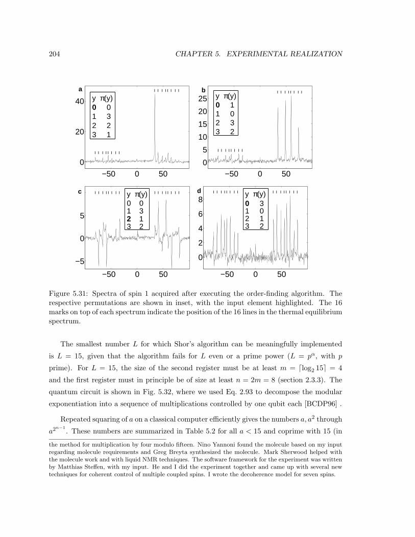
204 CHAPTER 5. EXPERIMENTAL REALIZATION
−50 0 50
0
20
40
− − − − − − − −
−−−−−−−−y π(y)0 01 32 23 1
a
−50 0 500
5
10
15
20
25
− − − − − − − −
−−−−−−−−
y π(y)0 11 02 33 2
b
−50 0 50
−5
0
5
− − − − − − − −−−−−−−−− y π(y)0 01 32 13 2
c
−50 0 50
0
2
4
6
8
− − − − − − − −−−−−−−−− y π(y)0 31 02 13 2
d
Figure 5.31: Spectra of spin 1 acquired after executing the order-finding algorithm. Therespective permutations are shown in inset, with the input element highlighted. The 16marks on top of each spectrum indicate the position of the 16 lines in the thermal equilibriumspectrum.
The smallest number L for which Shor’s algorithm can be meaningfully implemented
is L = 15, given that the algorithm fails for L even or a prime power (L = pα, with p
prime). For L = 15, the size of the second register must be at least m = dlog2 15e = 4
and the first register must in principle be of size at least n = 2m = 8 (section 2.3.3). The
quantum circuit is shown in Fig. 5.32, where we used Eq. 2.93 to decompose the modular
exponentiation into a sequence of multiplications controlled by one qubit each [BCDP96] .
Repeated squaring of a on a classical computer efficiently gives the numbers a, a2 through
a2n−1. These numbers are summarized in Table 5.2 for all a < 15 and coprime with 15 (in
the method for multiplication by four modulo fifteen. Nino Yannoni found the molecule based on my inputregarding molecule requirements and Greg Breyta synthesized the molecule. Mark Sherwood helped withthe molecule work and with liquid NMR techniques. The software framework for the experiment was writtenby Matthias Steffen, with my input. He and I did the experiment together and came up with several newtechniques for coherent control of multiple coupled spins. I wrote the decoherence model for seven spins.
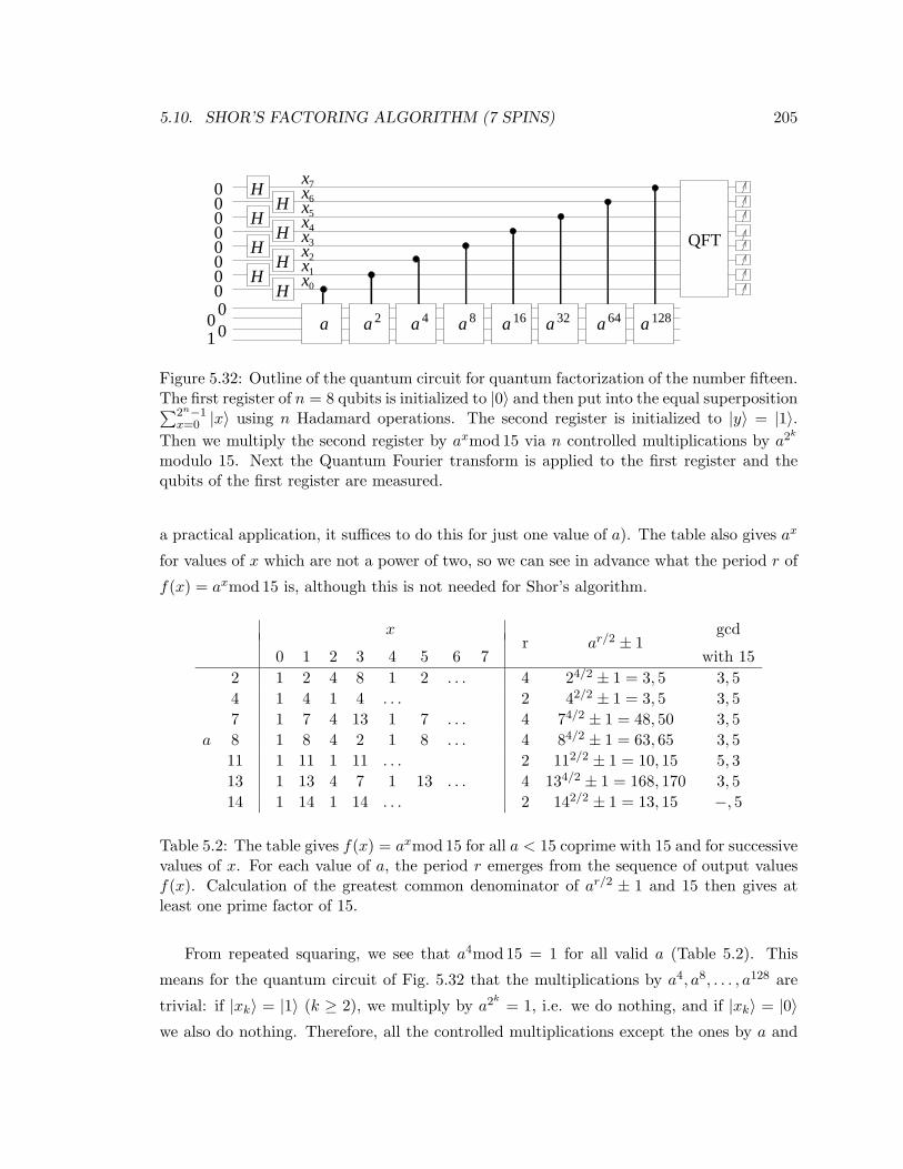
5.10. SHOR’S FACTORING ALGORITHM (7 SPINS) 205
a 2 84a 16 32aaa 64a 128aa
HH
HH
HH
HH
xxxxxxx
x0
1
2
3
4
5
6
700000
00
0
00
0
1
QFT
Figure 5.32: Outline of the quantum circuit for quantum factorization of the number fifteen.The first register of n = 8 qubits is initialized to |0〉 and then put into the equal superposition∑2n−1
x=0 |x〉 using n Hadamard operations. The second register is initialized to |y〉 = |1〉.Then we multiply the second register by axmod 15 via n controlled multiplications by a2k
modulo 15. Next the Quantum Fourier transform is applied to the first register and thequbits of the first register are measured.
a practical application, it suffices to do this for just one value of a). The table also gives ax
for values of x which are not a power of two, so we can see in advance what the period r of
f(x) = axmod 15 is, although this is not needed for Shor’s algorithm.
x gcd
0 1 2 3 4 5 6 7r ar/2 ± 1
with 152 1 2 4 8 1 2 . . . 4 24/2 ± 1 = 3, 5 3, 54 1 4 1 4 . . . 2 42/2 ± 1 = 3, 5 3, 57 1 7 4 13 1 7 . . . 4 74/2 ± 1 = 48, 50 3, 5
a 8 1 8 4 2 1 8 . . . 4 84/2 ± 1 = 63, 65 3, 511 1 11 1 11 . . . 2 112/2 ± 1 = 10, 15 5, 313 1 13 4 7 1 13 . . . 4 134/2 ± 1 = 168, 170 3, 514 1 14 1 14 . . . 2 142/2 ± 1 = 13, 15 −, 5
Table 5.2: The table gives f(x) = axmod 15 for all a < 15 coprime with 15 and for successivevalues of x. For each value of a, the period r emerges from the sequence of output valuesf(x). Calculation of the greatest common denominator of ar/2 ± 1 and 15 then gives atleast one prime factor of 15.
From repeated squaring, we see that a4mod 15 = 1 for all valid a (Table 5.2). This
means for the quantum circuit of Fig. 5.32 that the multiplications by a4, a8, . . . , a128 are
trivial: if |xk〉 = |1〉 (k ≥ 2), we multiply by a2k = 1, i.e. we do nothing, and if |xk〉 = |0〉we also do nothing. Therefore, all the controlled multiplications except the ones by a and

206 CHAPTER 5. EXPERIMENTAL REALIZATION
a2 can be left out. For a = 4, 11 or 14, we even have a2mod 15 = 1, so in this case we only
need to keep the controlled multiplication by a. We thus see that at most two qubits of
the first register act non-trivially during the modular exponentiation, and we might as well
leave out the other qubits altogether.16 Since the essence of Shor’s algorithm lies in the
interplay between modular exponentiation and the QFT, we chose to retain n = 3 qubits
to represent x.
In total, we shall thus use seven qubits (n = 3 and m = 4), as in Fig. 5.33. The possible
choices of a break down into two groups. The first group (a = 4, 11 and 14) is “easy” as
only multiplication by a is needed; we will refer to the second group (a = 2, 7, 8 and 13)
as the “difficult” case. We will implement the algorithm both for the easy and the difficult
case, using a = 11 and a = 7 respectively.
HH
H00
0
1000
xx
x0
1
2
a a 2
QFT1:2:3:4:5:6:7:
Figure 5.33: Simplified quantum circuit for quantum factorization of the number fifteen.
The controlled multiplications are done as follows. Multiplication of y = 1 by a is
equivalent to adding a − 1 to y = 1. The controlled multiplication by a can thus be
implemented via a few cnots of qubit 3 onto select qubits in the second register, as shown
in Fig. 5.34. Multiplication of y by 4 shifts the bits of y over two places:
y3 y2 y1 y0
× 4
y3 y2 y1 y0 0 0
In order to take the remainder of y3y2y1y000 divided by 15, we note that the weight of
bit y2 is now 16 and the weight of y3 is now 32; furthermore, we note that 16mod 15 = 1 and
that 32mod 15 = 2. In other words, y3y2y1y000 mod 15 = y1y0y3y2. In effect, multiplication
16In reality, if in the process of repeated squaring we find that a2kmod 15 = 1 for some k, while a2k−16= 1,
we know that the period r must be r = 2k. There is then really no need anymore to run the quantumalgorithm. This is the case for L = 15 for any choice of a. Nevertheless, the non-trivial operation of Shor’salgorithm can still be demonstrated [BCDP96].
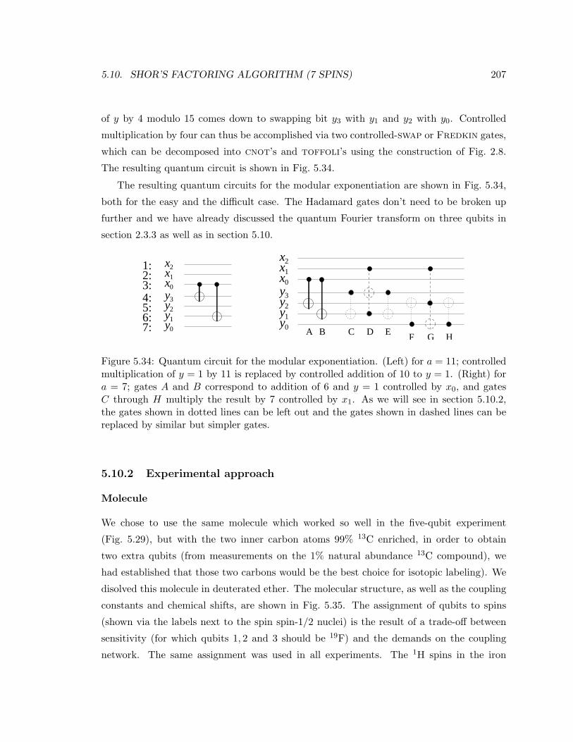
5.10. SHOR’S FACTORING ALGORITHM (7 SPINS) 207
of y by 4 modulo 15 comes down to swapping bit y3 with y1 and y2 with y0. Controlled
multiplication by four can thus be accomplished via two controlled-swap or Fredkin gates,
which can be decomposed into cnot’s and toffoli’s using the construction of Fig. 2.8.
The resulting quantum circuit is shown in Fig. 5.34.
The resulting quantum circuits for the modular exponentiation are shown in Fig. 5.34,
both for the easy and the difficult case. The Hadamard gates don’t need to be broken up
further and we have already discussed the quantum Fourier transform on three qubits in
section 2.3.3 as well as in section 5.10.
2xx1x0
y3yyy
2
1
0
1:2:3:4:5:6:7:
2xx1x0
y3yyy
2
1
0 A B C E G HFD
Figure 5.34: Quantum circuit for the modular exponentiation. (Left) for a = 11; controlledmultiplication of y = 1 by 11 is replaced by controlled addition of 10 to y = 1. (Right) fora = 7; gates A and B correspond to addition of 6 and y = 1 controlled by x0, and gatesC through H multiply the result by 7 controlled by x1. As we will see in section 5.10.2,the gates shown in dotted lines can be left out and the gates shown in dashed lines can bereplaced by similar but simpler gates.
5.10.2 Experimental approach
Molecule
We chose to use the same molecule which worked so well in the five-qubit experiment
(Fig. 5.29), but with the two inner carbon atoms 99% 13C enriched, in order to obtain
two extra qubits (from measurements on the 1% natural abundance 13C compound), we
had established that those two carbons would be the best choice for isotopic labeling). We
disolved this molecule in deuterated ether. The molecular structure, as well as the coupling
constants and chemical shifts, are shown in Fig. 5.35. The assignment of qubits to spins
(shown via the labels next to the spin spin-1/2 nuclei) is the result of a trade-off between
sensitivity (for which qubits 1, 2 and 3 should be 19F) and the demands on the coupling
network. The same assignment was used in all experiments. The 1H spins in the iron

208 CHAPTER 5. EXPERIMENTAL REALIZATION
complex broaden the lines of the nearest 13C spin, and were therefore decoupled during the
pulse sequence.
F
F F
FCF
C67
4
3
5
21
Fe
5 5C H CO
C
C
CO
T T J J J J
1 -22052.0 5.0 1.3 -221.0 37.7 6.6 -114.3 14.5 25.162 489.5 13.7 1.8 18.6 -3.9 2.5 79.9 3.9 3 25088.3 3.0 2.5 1.0 -13.5 41.6 12.94 -4918.7 10.0 1.7 54.1 -5.7 2.15 15186.6 2.8 1.8 19.4 59.5
7 4244.3 31.6 2.0
JJω
6 -4519.1 45.4 2.0 68.9
7i 6i 5i 4i 3i 2ii 1,i 2,ii
Figure 5.35: The seven spin molecule, along with the measured J-coupling constants [Hz],chemical shifts at 11.7 T [Hz] and relaxation time constants [s].
C13 C
OEtBr
H
HO
C13 C
OEt
HO
F
H C13 C
H
HO
F O Na- +
MoF6C13 C
H
F
F
F
C
F
F F
13C
C13 C
F
F
Fbp = 3-6C
AgF NaOH
C13 C
H
F
H
BuLi/hexane
THF
bp = -78C bp = -51C
BuLi/hexane
C13 C
F
F
F
-
bp = -26C
F
F
F
C13 C
F
F
F
I
bp = 30C
1) Zn2) Pd(Ph P)
3 4
distill
C
F
F F
13C
C13 C
F
FFe
[Fe(Cp)(CO) ]
Na(Hg)
THF
2 2
CpCO
CO
distill
2I
o
Figure 5.36: Schematic diagram of the synthesis of the seven-spin molecule.

5.10. SHOR’S FACTORING ALGORITHM (7 SPINS) 209
The synthesis of this unusual molecule was quite complex, and is summarized in Fig. 5.36.
Ethyl (2-13C)bromoacetate (Cambridge Isotopes) was converted to ethyl 2-fluoroacetate by
heating with AgF followed by hydrolysis to sodium fluoroacetate using NaOH in MeOH. The
resulting salt was converted to 1,1,1,2-tetrafluoroethane using MoF6 [dP79] and was subse-
quently treated with two equivalents of BuLi followed by I2 to provide trifluoroiodoethene
[BCHP96]. Half of the ethene was converted to the zinc salt which was recombined with
the remaining ethene and coupled using Pd(Ph3P)4 to give (2,3-13C)-hexafluorobutadiene
[JKB+87]. The end product was obtained by reacting this butadiene with the anion ob-
tained from treating [(p-C5H5)Fe(CO)2]2 with sodium amalgam [GMS68].
Input state preparation
For the creation of an effective pure state of all seven spins, we used a two-stage extension
of the scheme used in the five-spin experiment. In the first stage, the five fluorine spins are
made effective pure via summation of the nine experiments of Table 5.3, where the first five
qubits are fluorine spins and the last two are carbons.
Equilibrium ZIIIIII IZIIIII IIZIIII IIIZIII IIIIZII1. C24C12C31C51 ZIIZZII ZZZZZII ZIZZZII −IIZIIII IIIIZII2. C35C43C14N2 ZIIIIII ZZIIIII −IIZIIII ZZIZZII ZZIIZII3. C43C14C21C31N5 ZIZIZII ZZZIZII IIZIIII −IIIZIII ZZZIIII4. C42C14C51C21N1N5 ZIZZIII ZZIZIII ZZZZIZZ −IIIZIII IIIIZII5. C35C43C24C35 ZIIIIII IZZIIII IIZIIII IZZZIII IZZIZII6. C13C15C21C12 ZIZIIII IZIIIII IIZIIII IIZZIII IIZIZII7. C42C34C53C31 ZIIIZII IZIZZII IZZZZII IIIZIII IIIZZII8. C42C34C53C42C34N1 −ZIIIIII IZIZIII IIZZZII IIIZIII IIIZZII9. C35C34C51N4N2N3 ZIIZIII IZIIZII −IIZIIII −IIIZZII −IIIIZII
Table 5.3: First stage of the temporal averaging procedure to prepare an effective purestate of five nuclei of the same species and two other nuclei of another species. The tableshows how the terms in the thermal equilibrium density matrix are transformed by eachtemporal averaging sequence (the IIIIIZI and IIIIIIZ terms are not shown as they areleft unaffected in this first stage). Cij stands for cnotij and Ni stands for noti.
These state preparation sequences were designed to be as short as possible by making
optimal use of the available coupling network. The nine experiments are repeated four
times, each time with different additional operations. In this process, all except four of the
IIIIIZI and IIIIIIZ terms are averaged away (these terms have about one fourth the
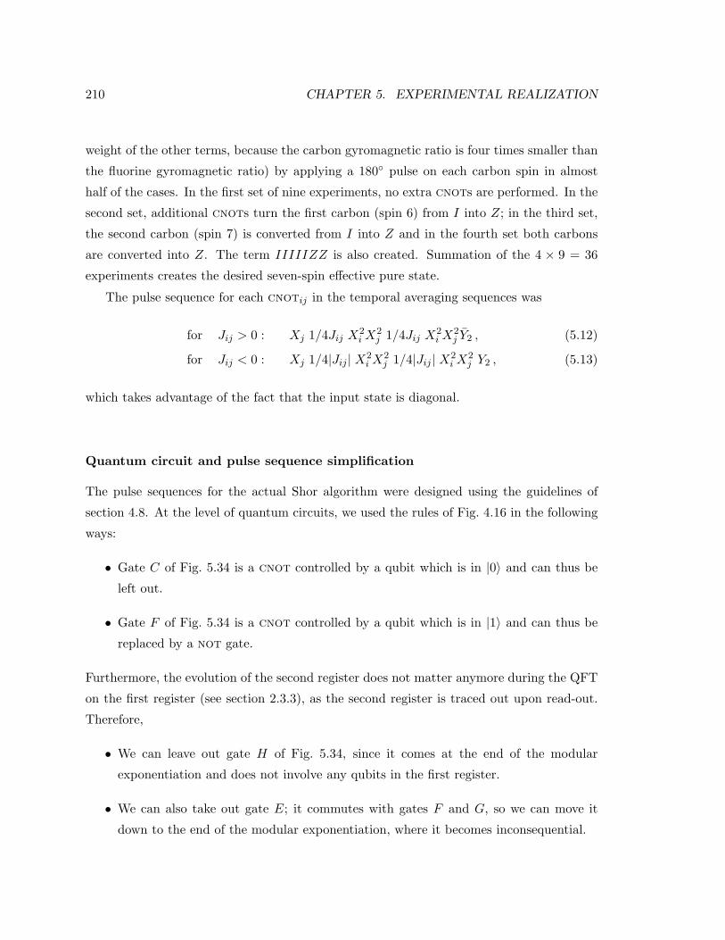
210 CHAPTER 5. EXPERIMENTAL REALIZATION
weight of the other terms, because the carbon gyromagnetic ratio is four times smaller than
the fluorine gyromagnetic ratio) by applying a 180 pulse on each carbon spin in almost
half of the cases. In the first set of nine experiments, no extra cnots are performed. In the
second set, additional cnots turn the first carbon (spin 6) from I into Z; in the third set,
the second carbon (spin 7) is converted from I into Z and in the fourth set both carbons
are converted into Z. The term IIIIIZZ is also created. Summation of the 4 × 9 = 36
experiments creates the desired seven-spin effective pure state.
The pulse sequence for each cnotij in the temporal averaging sequences was
for Jij > 0 : Xj 1/4Jij X2iX
2j 1/4Jij X2
iX2j Y2 , (5.12)
for Jij < 0 : Xj 1/4|Jij | X2iX
2j 1/4|Jij | X2
iX2j Y2 , (5.13)
which takes advantage of the fact that the input state is diagonal.
Quantum circuit and pulse sequence simplification
The pulse sequences for the actual Shor algorithm were designed using the guidelines of
section 4.8. At the level of quantum circuits, we used the rules of Fig. 4.16 in the following
ways:
• Gate C of Fig. 5.34 is a cnot controlled by a qubit which is in |0〉 and can thus be
left out.
• Gate F of Fig. 5.34 is a cnot controlled by a qubit which is in |1〉 and can thus be
replaced by a not gate.
Furthermore, the evolution of the second register does not matter anymore during the QFT
on the first register (see section 2.3.3), as the second register is traced out upon read-out.
Therefore,
• We can leave out gate H of Fig. 5.34, since it comes at the end of the modular
exponentiation and does not involve any qubits in the first register.
• We can also take out gate E; it commutes with gates F and G, so we can move it
down to the end of the modular exponentiation, where it becomes inconsequential.

5.10. SHOR’S FACTORING ALGORITHM (7 SPINS) 211
Furthermore, we took advantage of the fact that the target of the two Toffoli’s (gates
D and G in Fig. 5.34) are in a computational basis state, not in a superposition state.
Therefore, the phases of only half the non-zero entries in the Toffoli unitary matrices
need to be the same, and we can use a simplified set of gates to implement them.
Y Z 2 Y
Y Z 2 Y
DB A
y3yyy
2
1
0
2xx1x0
F G
Figure 5.37: Simplified quantum circuit for the modular exponentiation for the “difficult”case (a = 7).
In addition, we simplified the refocusing schemes in two ways. Early on in the pulse
sequence, certain spins in the second register are still in |0〉 or |1〉, and the couplings between
any two such spins need not be refocused. In order to maximally take advantage of this
simplification, gate A was performed after gate E. This is allowed since A commutes with B,
C, D and E. During the QFT, the evolution of the second register does not matter anymore,
so the couplings between the spins in the second register need not be refocused during the
QFT (couplings between the first and second register qubits must still be refocused). We
did refocus inhomogeneous dephasing for all spins in the transverse plane at all times.
The quantum circuit resulting from these various simplifications is shown in Fig. 5.37.
Spectrometer
The four-channel spectrometer was converted into a seven-channel spectrometer using the
same approach as for the five-qubit experiment of section 5.9: additional rotating reference
frames were created using a software time counter, and phase ramping techniques enabled
excitation of spins away from the signal source frequency. The frequency source of channel
1 was placed at ω1, on resonance with spin 1, source 2 was set at (ω2 + ω4)/2, source 3
at (ω3 + ω5)/2 and source 4 at (ω6 + ω7)/2. In addition, we installed an extra frequency
source, power amplifier and power combiner for proton decoupling.
We selected Hermite 180 and Gaussian 90 pulse shapes based on our previous experience,

212 CHAPTER 5. EXPERIMENTAL REALIZATION
collected in Table 4.2, and on the spectral properties of the molecule and the demands of
the algorithms. Generalized Bloch-Siegert effects were precomputed and compensated for,
both for single (section 4.2.4) and simultaneous (section 4.2.5) pulses. Simultaneous pulses
on strongly coupled spins were avoided. Furthermore, coupled evolution during the pulses
was unwound using symmetrically placed negative delay times, following the guidelines of
Table 4.3 for single pulses and Table 4.4 for simultaneous pulses.
The complete pulse sequence for the difficult case contains about 300 180 pulses and
about 30 90 pulses. The duration of the temporal averaging part is on the order of 200
ms, the modular exponentiation takes about 400 ms, and the QFT sequence lasts about
120 ms.
Read-out
Upon completion of the pulse sequence, the reduced density matrix of the three qubits in
the first register is predicted to be
ρ =∑l
wl|lN/r〉〈lN/r| =∑l
wl|l 8r 〉〈l8r | (5.14)
We shall attempt to deduce r from the output spectra of the first three qubits, after a
readout pulse, which represent bitwise ensemble averaged values. Once r is known, we can
find the prime factors of L = 15 as (recall Eq. 2.91)
gcd(ar/2 ± 1, 15) . (5.15)
5.10.3 Experimental results
Fig. 5.38 shows the thermal equilibrium fluorine spectrum of the sample. Fig. 5.39 zooms in
on five of the lines in this spectrum, corresponding to the five fluorine spins of the quantum
computer molecule of Fig. 5.35. Fig. 5.40 shows the spectra of the two carbon spins.
Each multiplet contains up to 26 = 64 lines, because each spin is coupled to six other
spins. For spin 1, all 64 lines are beautifully resolved. For the other spins, some of the
lines fall on top of each other, but this does not pose a problem since at the end of a Shor’s
algorithm we only need to know the overall signature: lines up, lines down, or partly up /
partly down.
5.10. SHOR’S FACTORING ALGORITHM (7 SPINS) 213
Figure 5.38: Fluorine spectrum of the seven-spin molecule of Fig. 5.35. The five major linescorrespond )from left to right) to qubits 1, 4, 2, 5, 3. In addition, two smaller lines fromimpurities are visible around 25 kHz. The spectrum is shown in absolute value. Frequenciesare given in kHz, with respect to an arbitrary reference frequency near 470 MHz.
The spectra of spins 1, 2 and 3 after preparing a seven-spin effective pure ground state
are shown in Fig. 5.41. These spectra are the summation of 36 spectra, each obtained after
a different input state preparation pulse sequence. As expected, only one line is retained
in each multiplet, which indicates that we have distilled a suitable initial state for Shor’s
algorithm.
The experimentally measured spectra upon completion of the “easy” case of Shor’s
algorithm are shown in Fig. 5.42. Clearly, the lines of spins 1 and 2 are up, so qubits 1
and 2 are in |0〉; qubit 3 is in a mixture of |0〉 and |1〉 as it has positive and negative lines.
With qubit 3 the most significant qubit after the QFT [Cop94], the first register is thus
in a mixture of |000〉 and |100〉, or |0〉 and |4〉 in decimal notation. The periodicity in the
amplitude of |x〉 is thus 4, and therefore r = 8/4 = 2. If we plug this in in Eq. 5.15, we
obtain gcd(112/2 ± 1, 15) = 3, 5. The prime factors of 15 have thus been unambiguously
derived from the output spectra.
Similar spectra for the “difficult” case are shown in Fig. 5.43. From the spectra, we
conclude that qubit 1 is in |0〉, and qubits 2 and 3 are in a mixture of |0〉 and |1〉. The
register is thus in a mixture of |000〉, |010〉, |100〉 and |110〉, which in decimal is |0〉, |2〉,|4〉 and |6〉. The periodicity in the amplitude of the first register is thus 2, and therefore
r = 8/2 = 4. Plugging this in in Eq. 5.15 gives gcd(74/2 ± 1, 15) = 3, 5. Even after the very
long pulse sequence of the “difficult” case, the prime factors of 15 have thus successfully
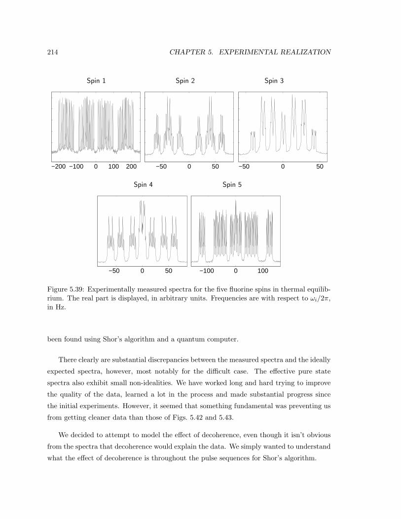
214 CHAPTER 5. EXPERIMENTAL REALIZATION
Spin 1 Spin 2 Spin 3
−200 −100 0 100 200 −50 0 50 −50 0 50
Spin 4 Spin 5
−50 0 50 −100 0 100
Figure 5.39: Experimentally measured spectra for the five fluorine spins in thermal equilib-rium. The real part is displayed, in arbitrary units. Frequencies are with respect to ωi/2π,in Hz.
been found using Shor’s algorithm and a quantum computer.
There clearly are substantial discrepancies between the measured spectra and the ideally
expected spectra, however, most notably for the difficult case. The effective pure state
spectra also exhibit small non-idealities. We have worked long and hard trying to improve
the quality of the data, learned a lot in the process and made substantial progress since
the initial experiments. However, it seemed that something fundamental was preventing us
from getting cleaner data than those of Figs. 5.42 and 5.43.
We decided to attempt to model the effect of decoherence, even though it isn’t obvious
from the spectra that decoherence would explain the data. We simply wanted to understand
what the effect of decoherence is throughout the pulse sequences for Shor’s algorithm.

5.10. SHOR’S FACTORING ALGORITHM (7 SPINS) 215
Spin 6 Spin 7
−150 0 150 −75 0 75
Figure 5.40: Experimentally measured spectra for the two carbon spins in thermal equilib-rium. The real part is displayed, in arbitrary units. Frequencies are with respect to ωi/2π,in Hz.
Spin 1 Spin 2 Spin 3
−200 −100 0 100 200 −50 0 50 −50 0 50
Figure 5.41: Experimentally measured spectra, similar to Fig. 5.39, after preparing all sevenspins in the effective pure ground state.
5.10.4 Decoherence model
The NMR literature gives very detailed descriptions of decoherence in coupled spin systems,
going back to the ideas of Redfield [Red57, Red65] and worked out later by many others
[VV78, Jee82, EBW87]. This so-called superoperator formalism is very general and allows
one to simulate decoherence in nuclear spin systems starting from knowledge of internu-
clear distances, chemical shift anisotropy tensors, and so forth, and of correlations of these
mechanism in time and space, which are governed by molecular tumbling and diffusion
rates. While such calculations are in principle amenable to computer simulations, detailed
knowledge about the correlation functions and the other parameters is not always available.
Furthermore, a full superoperator description of relaxation is exceedingly complex for the
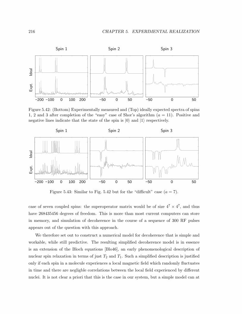
216 CHAPTER 5. EXPERIMENTAL REALIZATION
Spin 1 Spin 2 Spin 3
Exp
t.Id
eal
−200 −100 0 100 200 −50 0 50 −50 0 50
Figure 5.42: (Bottom) Experimentally measured and (Top) ideally expected spectra of spins1, 2 and 3 after completion of the “easy” case of Shor’s algorithm (a = 11). Positive andnegative lines indicate that the state of the spin is |0〉 and |1〉 respectively.
Spin 1 Spin 2 Spin 3
Exp
t.Id
eal
−200 −100 0 100 200 −50 0 50 −50 0 50
Figure 5.43: Similar to Fig. 5.42 but for the “difficult” case (a = 7).
case of seven coupled spins: the superoperator matrix would be of size 47 × 47, and thus
have 268435456 degrees of freedom. This is more than most current computers can store
in memory, and simulation of decoherence in the course of a sequence of 300 RF pulses
appears out of the question with this approach.
We therefore set out to construct a numerical model for decoherence that is simple and
workable, while still predictive. The resulting simplified decoherence model is in essence
is an extension of the Bloch equations [Blo46], an early phenomenological description of
nuclear spin relaxation in terms of just T2 and T1. Such a simplified description is justified
only if each spin in a molecule experiences a local magnetic field which randomly fluctuates
in time and there are negligble correlations between the local field experienced by different
nuclei. It is not clear a priori that this is the case in our system, but a simple model can at
5.10. SHOR’S FACTORING ALGORITHM (7 SPINS) 217
least serve to give a first idea of the impact of decoherence during the execution of Shor’s
algorithm. Comparison of the simulation results with the experimental data will reveal the
usefulness of this simplified model.
In order to make the model easily compatible with our matrix formalism for unitary
operations (section 2.2), we chose to describe decoherence in the operator sum representation
or Kraus representation [Kra83]. The operator sum representation of both generalized
amplitude damping (T1) and phase damping (related to T2) has been described in the
quantum computing literature [NC00] (see also section 3.1.5), although only for single spins,
and for both processes separately.
We have devised and implemented an integrated model of phase damping and generalized
amplitude damping acting on seven coupled spins in the course of arbitrary pulse sequences.
We have been able to keep the model workable by assuming that each spin decoheres
independently and by making the following observations:
1. Amplitude damping error operators acting on different spins commute.
2. Phase damping error operators acting on different spins commute.
3. Amplitude damping and phase damping commute with each other. This follows from
the fact that the error operators Ei for amplitude damping (Eq. 3.20) commute with
the Ei for phase damping (Eq. 3.26) when applied to σx, σy, σz and σI and thus also
when they act on arbitrary ρ.
4. Phase damping commutes with the ideal unitary evolution under H, as both processes
are described by diagonal matrices.
As a result, there is no need to simulate all these processes simultaneously; they can
be simulated one after the other, in any order. This prevents an explosion of terms in the
operator sum representation, which would have been the case if cross-products of all the Eihad been required. However,
1. Amplitude damping does not commute with the ideal unitary evolution under H.
2. Phase and amplitude damping do not commute with the ideal unitary evolution during
RF pulses.

218 CHAPTER 5. EXPERIMENTAL REALIZATION
In order to still maintain a workable model, we have nevertheless treated these processes
as if they did commute. This is not necessarily a good approximation, but it does allow us
to get a first estimate of the effect of decoherence.
Concretely, we modeled a delay time of duration t via e−iHt/~ followed by amplitude
damping acting on spin 1 for a duration t, then amplitude damping acting on spin 2 and
so forth, followed by phase damping acting for the same duration on each spin one after
the other. Similarly, a shaped pulse of duration pw was modeled via an ideal shaped pulse,
preceeded by amplitude damping and phase damping, acting on each spin separately for a
duration pw. Thanks to these approximations, the simulation of the complete Shor pulse
sequence, including 36 temporal averaging sequences, takes only a few minutes to run on four
IBM power3-II processors. We measured the characteristic amplitude and phase damping
time constants for each spin and plugged those values into the model (excerpts from the
simulation code are given in Appendix A). The model thus has no free parameters.
The output spectra obtained from the simulation are shown in Figs. 5.44 and 5.45 for
the easy and difficult case respectively, along with the experimental output spectra. In both
cases, the model reproduced the main unexpected observed non-idealities in the data in a
remarkably convincing manner.
Spin 1 Spin 2 Spin 3
Exp
t.S
imu
l.
−200 −100 0 100 200 −50 0 50 −50 0 50
Figure 5.44: Comparison between (bottom) the experimentally measured spectra, whichare the same as in Fig. 5.42, and (top) simulated spectra based on the decoherence model,for the “easy” case (a = 11).
The good agreement between the spectra predicted by the relaxation model and the
experimental spectra suggests that the assumptions underlying the model are valid, at
least to a reasonable degree. We attribute the remaining discrepancies between the data
and the simulations to the approximations made in the model as well as to experimental

5.11. SUMMARY 219
Spin 1 Spin 2 Spin 3E
xpt.
Sim
ul.
−200 −100 0 100 200 −50 0 50 −50 0 50
Figure 5.45: Similar to Fig. 5.44 but for the “hard” case (a = 7).
imperfections such as RF inhomogeneity, imperfect calibrations and incomplete unwinding
of coupled evolution during the pulses.
5.10.5 Discussion
The prime factors of fifteen can be deduced from the output spectra, both for the easy and
the difficult case, demonstrating the proper operation of the factoring algorithm. This is in
itself really remarkable.
The unexpected non-idealities in the data are well reproduced by a simple numeric model
that incorporates the effect of decoherence. This is the first NMR quantum computing
experiment in which decoherence was the dominant source of errors; the demands of Shor’s
algorithm are clearly pushing the limits of the current molecule, despite its exceptionally
good properties. Certainly, the predictive but workable decoherence model for multiple
coupled spins is a valuable tool to assess the feasability of future NMR quantum computing
experiments.
Finally, the good agreement between the measured and simulated spectra suggests that
the degree of unitary control in the experiment was very high, which bodes well for related
proposed implementations of quantum computers [Kan98, LD98].
5.11 Summary
The sequence of successful experiments presented in this chapter clearly demonstrate that
nuclear spins in liquid solution represent a beautiful playground in which to explore quantum
220 CHAPTER 5. EXPERIMENTAL REALIZATION
computing experimentally. The main results of these experiments are
• experimental proof of principle of quantum computing — the solution of mathematical
problems in fewer steps than is possible with any classical machine,
• experimental proof of principle of quantum error detection — coding gives a first order
improvement in the conditional fidelity,
• an explicit demonstration of zero temperature dynamics with room temperature nu-
clear spins,
• the observation of a surprisingly large degree of cancellation of systematic errors —
the concatenation of a record 280 two-qubit gates on three spins,
• a demonstration that liquid crystal solvents can be used for NMR quantum computing
— such solvents may allow more gates within the coherence time,
• the demonstration of coherent control over up to seven coupled nuclear spins over the
course of tens of two-qubit gates,
• the demonstration of a workable yet predictive model of decoherence for seven coupled
nuclear spins.
The main experimental challenges we had to address in the course of these experiments
include
• the identification and synthesis of suitable molecules,
• the exponential overhead in the creation of effective pure states,
• the limitations of a four-channel spectrometer,
• ”turning off” undesired terms in the Hamiltonian, which is especially tricky if they
don’t commute with the desired terms,
• developing predictive numerical models of unitary and non-unitary spin dynamics.
Despite the successful resolution of these challenges in our experiments, liquid NMR
quantum computers are difficult to scale, in particular because of the exponential overhead
5.11. SUMMARY 221
in the input state preparation. It also appears unlikely that the accuracy threshold for fault-
tolerant quantum computation can be reached, except perhaps for very small molecules.
Nevertheless, full quantum algorithms with 10-15 spins may be possible, and interest-
ing demonstrations of coherent control over several dozens of spins may be possible using
thermal input states. Certainly, nuclear spins in liquid solution will continue to provide an
exciting and accessible avenue to study quantum computation experimentally.

Chapter 6
Conclusions
Quantum computation has now entered the realm of experimental reality: simple quantum
computers based on nuclear spins in molecules have been used to solve problems in fewer
steps than is possible with any classical device. We have continuously been pushing the state
of the art in NMR quantum computing by implementing meaningful quantum algorithms
on two, then three, later five and finally seven qubits. In these experiments, we have not
been content with just the simplest quantum protocols requiring only nearest neighbour
couplings, but instead chose realistic experiments which really put the quantum computers
to test.
In order to make this possible, special molecules were synthesized and a large number of
experimental techniques have been developed for state initialization, coherent control and
read-out. These include more efficient and effective temporal averaging schemes for state
preparation, methods to reduce cross-talk during spin-selective shaped pulses, methods
to reduce cross-talk between shaped pulses on different spins, the uncoupling frame for
automatic refocusing within a subspace, pulse sequence simplification procedures at various
levels, software rotating reference frames, refocusing schemes to remove undesired terms in
the Hamiltonian, ways to interpret ensemble averaged measurements, and readout schemes
based on the multiplet fine structure.
We have gained a good understanding of the main sources of imperfections in the ex-
periments by developing a set of practical and predictive simulation tools which allow us to
model both unitary and decoherence processes for molecules with multiple coupled nuclear
spins. In the early heteronuclear experiments, RF field inhomogeneity was the dominant
222
223
source of errors. In the later homonuclear experiments, which require longer pulses, cou-
pled evolution during the RF pulses became the most significant source of errors. Other
sources of errors included imperfect calibrations, incomplete frequency drift compensation
and limited signal-to-noise. All these imperfections arise from technological rather than
from fundamental issues, and we have demonstrated that such systematic errors can be
cancelled out to a great extent. Even though intrinsic decoherence played a role in all the
experiments, only in the last experiment did decoherence become the dominant source of
errors.
There exist well-understood scaling limitations for nuclear spin quantum computers
starting off in thermal equilibrium at room temperature. Most importantly, the probability
that all spins in a quantum computer with n spins starts off in the desired ground state de-
creases as n/2n. While a subset of the spins can be efficiently cooled down algorithmically,
the overhead for this procedure is impractically large unless substantial hyperpolarization
of the nuclear spins can be achieved by other means. An additional problem is that the
coherence time of nuclear spins in molecules tends to shorten as the number of spins in-
creases.
Nevertheless, I am convinced that solution NMR quantum computing will continue
to help address many open problems and unanswered questions (and raise many more).
Those questions include very fundamental ones, such as “where does the power of quantum
computing come from?”. But as quantum computation has become an experimental reality,
many important open problems are practical ones. (1) How can we remove the effect of
undesired terms in the Hamiltonian via an approach that is both general and practical?
(2) How do we arrange the sequence of operations in a systematic way, so as to maximize
the cancellation of systematic errors? (3) How do we create and validate practical and
predictive decoherence models?
The work presented in this thesis work constitutes a first step towards answering these
important questions, but it represents by no means an endpoint. The significance of the
practical open problems will only increase as other, perhaps more scalable implementations
of quantum computers reach the stage of realizing actual quantum computations. Similarly,
I hope that the significance of the techniques and concepts we developed for NMR quan-
tum computing will grow, as they find useful application in other realizations of quantum
computers.
Both the questions and the answers which stemmed from the work on NMR quantum

224 CHAPTER 6. CONCLUSIONS
computers have tremendously increased our understanding of what it takes to build a quan-
tum computer. Still, the big question we asked in the beginning remains open: can we build
a practical quantum computer?
This question can only be answered by measuring the coherence time and developing
techniques for initialization, control and read-out of the qubit states in a variety of potential
embodiments of quantum computers. The fundamental requirement for any implementation
is that the accuracy threshold for fault-tolerant quantum computation be reached1. Specif-
ically, the probability of error per elementary logic gate should be less than about 0.01 %,
in the most optimistic estimates at present. It is clear that reaching the accuracy threshold
represents a formidable challenge; it requires not only coherence times long compared to
the gate times, but also extremely accurate unitary control over the qubits. Nevertheless,
0.01 % doesn’t seem a priori impossible, and in the spirit of Feynman, we say:
We know of no laws of physics that prohibit practical quantum computers — we
just haven’t gotten around to building one . . .
Therefore, while I don’t believe that horses can be made to fly, I do think that practical
quantum computers may one day be built. It is my hope and expectation that this thesis
work has contributed to the realization of this wonderful challenge, which holds such a great
promise.
1In order to perform meaningful quantum computations without using quantum error correction, theprobability of error should be even lower, so the accuracy threshold is a reasonable upper bound for theerror rate.

Appendix A
Numerical model
The MATLAB model for simulation of the unitary and non-unitary processes in the course
of a pulse sequence contains four primitives:
1. d.m: free evolution under the Hamiltonian
2. X.m, Y.m and Z.m: ideal single-spin rotations
3. gad7.m: generalized amplitude damping (GAD)
4. pd7.m: phase damping (PD)
The last two programs, which model non-unitary processes, act directly on a density
matrix. The programs for unitary processes act on density matrices via the program rho.m.
The simulation programs require that the number of qubits nq be declared in advance, and
that the Hamiltonian and the Pauli matrices be set up by calling def.m.
In the next subsections, we shall give excerpts from the MATLAB code of def.m, rho.m,
d.m, X.m, gad7.m and pd7.m and two helper programs. Finally, we will give an excerpt from
a pulse sequence which calls these primitives.
A.1 Set up the Hamiltonian and Pauli matrices
% File: def.m% Date: 1997% Author: Lieven Vandersypen <[email protected]>
225
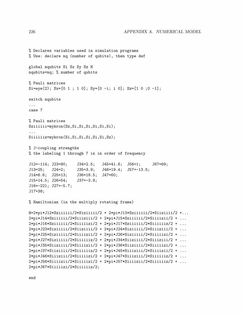
226 APPENDIX A. NUMERICAL MODEL
% Declares variables used in simulation programs% Use: declare nq (number of qubits), then type def
global nqubits Si Sx Sy Sz Hnqubits=nq; % number of qubits
% Pauli matricesSi=eye(2); Sx=[0 1 ; 1 0]; Sy=[0 -i; i 0]; Sz=[1 0 ;0 -1];
switch nqubits...case 7
% Pauli matricesSziiiiii=mykron(Sz,Si,Si,Si,Si,Si,Si);...Siiiiiiz=mykron(Si,Si,Si,Si,Si,Si,Sz);
% J-coupling strengths% the labeling 1 through 7 is in order of frequency
J12=-114; J23=80; J34=2.5; J45=41.6; J56=1; J67=69;J13=25; J24=2; J35=3.9; J46=19.4; J57=-13.5;J14=6.6; J25=13; J36=18.5; J47=60;J15=14.5; J26=54; J37=-3.8;J16=-221; J27=-5.7;J17=38;
% Hamiltonian (in the multiply rotating frame)
H=2*pi*J12*Sziiiiii/2*Siziiiii/2 + 2*pi*J13*Sziiiiii/2*Siiziiii/2 +...2*pi*J14*Sziiiiii/2*Siiiziii/2 + 2*pi*J15*Sziiiiii/2*Siiiizii/2 + ...2*pi*J16*Sziiiiii/2*Siiiiizi/2 + 2*pi*J17*Sziiiiii/2*Siiiiiiz/2 + ...2*pi*J23*Siziiiii/2*Siiziiii/2 + 2*pi*J24*Siziiiii/2*Siiiziii/2 + ...2*pi*J25*Siziiiii/2*Siiiizii/2 + 2*pi*J26*Siziiiii/2*Siiiiizi/2 + ...2*pi*J27*Siziiiii/2*Siiiiiiz/2 + 2*pi*J34*Siiziiii/2*Siiiziii/2 + ...2*pi*J35*Siiziiii/2*Siiiizii/2 + 2*pi*J36*Siiziiii/2*Siiiiizi/2 + ...2*pi*J37*Siiziiii/2*Siiiiiiz/2 + 2*pi*J45*Siiiziii/2*Siiiizii/2 + ...2*pi*J46*Siiiziii/2*Siiiiizi/2 + 2*pi*J47*Siiiziii/2*Siiiiiiz/2 + ...2*pi*J56*Siiiizii/2*Siiiiizi/2 + 2*pi*J57*Siiiizii/2*Siiiiiiz/2 + ...2*pi*J67*Siiiiizi/2*Siiiiiiz/2;
end
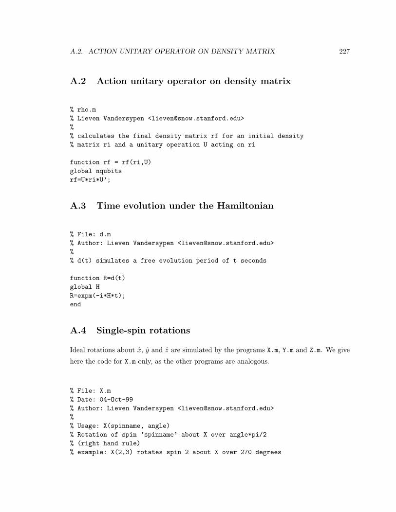
A.2. ACTION UNITARY OPERATOR ON DENSITY MATRIX 227
A.2 Action unitary operator on density matrix
% rho.m% Lieven Vandersypen <[email protected]>%% calculates the final density matrix rf for an initial density% matrix ri and a unitary operation U acting on ri
function rf = rf(ri,U)global nqubitsrf=U*ri*U’;
A.3 Time evolution under the Hamiltonian
% File: d.m% Author: Lieven Vandersypen <[email protected]>%% d(t) simulates a free evolution period of t seconds
function R=d(t)global HR=expm(-i*H*t);end
A.4 Single-spin rotations
Ideal rotations about x, y and z are simulated by the programs X.m, Y.m and Z.m. We give
here the code for X.m only, as the other programs are analogous.
% File: X.m% Date: 04-Oct-99% Author: Lieven Vandersypen <[email protected]>%% Usage: X(spinname, angle)% Rotation of spin ’spinname’ about X over angle*pi/2% (right hand rule)% example: X(2,3) rotates spin 2 about X over 270 degrees

228 APPENDIX A. NUMERICAL MODEL
function X=X(spinname,angle)
global nqubits
if nargin == 1if nqubits == 1
angle=spinname; spinname=1;else
error(’X.m requires two arguments if nqubits > 1 !’)end
end
operator=expm(-i*angle*pi/2*[0 1;1 0]/2); % calculate 1-spin operatorX=gop(spinname,operator); % turns 1-spin operator into n-spin operator
A.5 Generalized amplitude damping
% file: gad7.m% April 2001% Lieven Vandersypen <[email protected]>%% simulate generalized amplitude damping (GAD), 7 spins% model assumes no correlation of GAD on different spins%% Usage rout=gad(rin,p,t,ratio)%% rin initial density matrix% p equilibrium polarization% t duration for which GAD acts% ratio set this to 1 to simulate GAD, set this to say 1e9 to% simulate the same sequence without GAD% rout final density matrix
function rout=gad(rin,p,t,ratio)
T1_1=ratio(1)*5.0; % the labeling is in order of frequencyT1_2=ratio(1)*10.0;T1_3=ratio(1)*13.7;T1_4=ratio(1)*2.8;T1_5=ratio(1)*3.0;
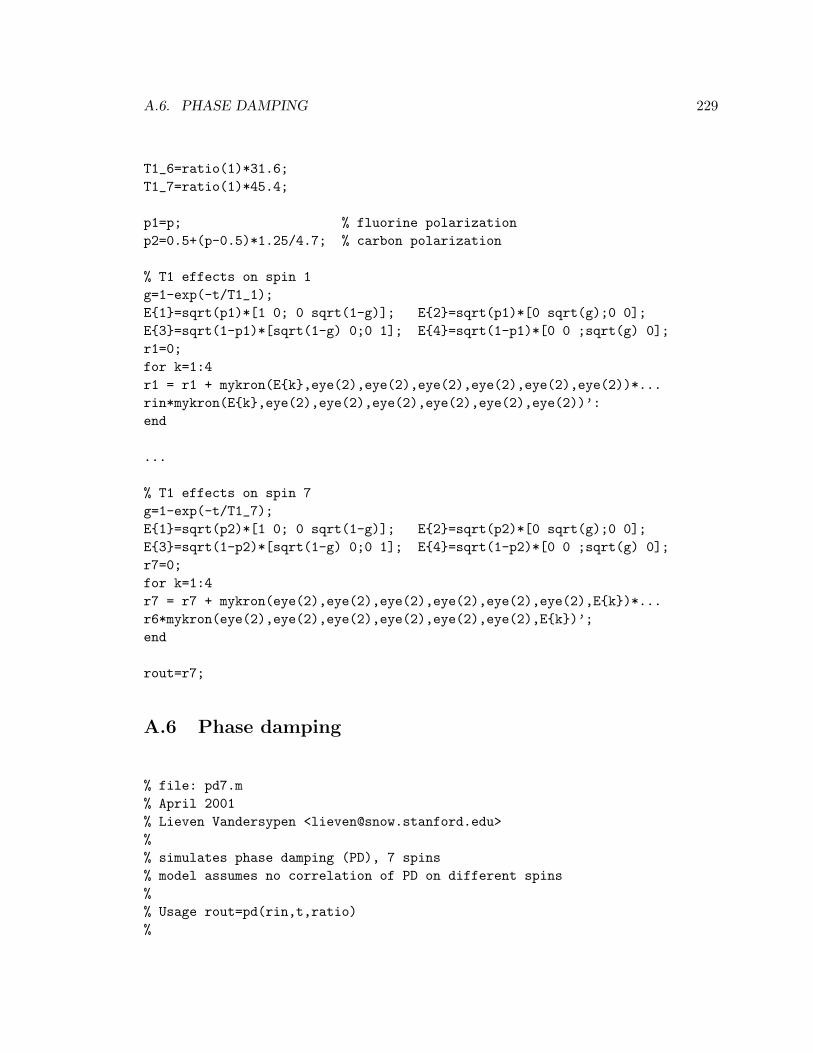
A.6. PHASE DAMPING 229
T1_6=ratio(1)*31.6;T1_7=ratio(1)*45.4;
p1=p; % fluorine polarizationp2=0.5+(p-0.5)*1.25/4.7; % carbon polarization
% T1 effects on spin 1g=1-exp(-t/T1_1);E1=sqrt(p1)*[1 0; 0 sqrt(1-g)]; E2=sqrt(p1)*[0 sqrt(g);0 0];E3=sqrt(1-p1)*[sqrt(1-g) 0;0 1]; E4=sqrt(1-p1)*[0 0 ;sqrt(g) 0];r1=0;for k=1:4r1 = r1 + mykron(Ek,eye(2),eye(2),eye(2),eye(2),eye(2),eye(2))*...rin*mykron(Ek,eye(2),eye(2),eye(2),eye(2),eye(2),eye(2))’:end
...
% T1 effects on spin 7g=1-exp(-t/T1_7);E1=sqrt(p2)*[1 0; 0 sqrt(1-g)]; E2=sqrt(p2)*[0 sqrt(g);0 0];E3=sqrt(1-p2)*[sqrt(1-g) 0;0 1]; E4=sqrt(1-p2)*[0 0 ;sqrt(g) 0];r7=0;for k=1:4r7 = r7 + mykron(eye(2),eye(2),eye(2),eye(2),eye(2),eye(2),Ek)*...r6*mykron(eye(2),eye(2),eye(2),eye(2),eye(2),eye(2),Ek)’;end
rout=r7;
A.6 Phase damping
% file: pd7.m% April 2001% Lieven Vandersypen <[email protected]>%% simulates phase damping (PD), 7 spins% model assumes no correlation of PD on different spins%% Usage rout=pd(rin,t,ratio)%
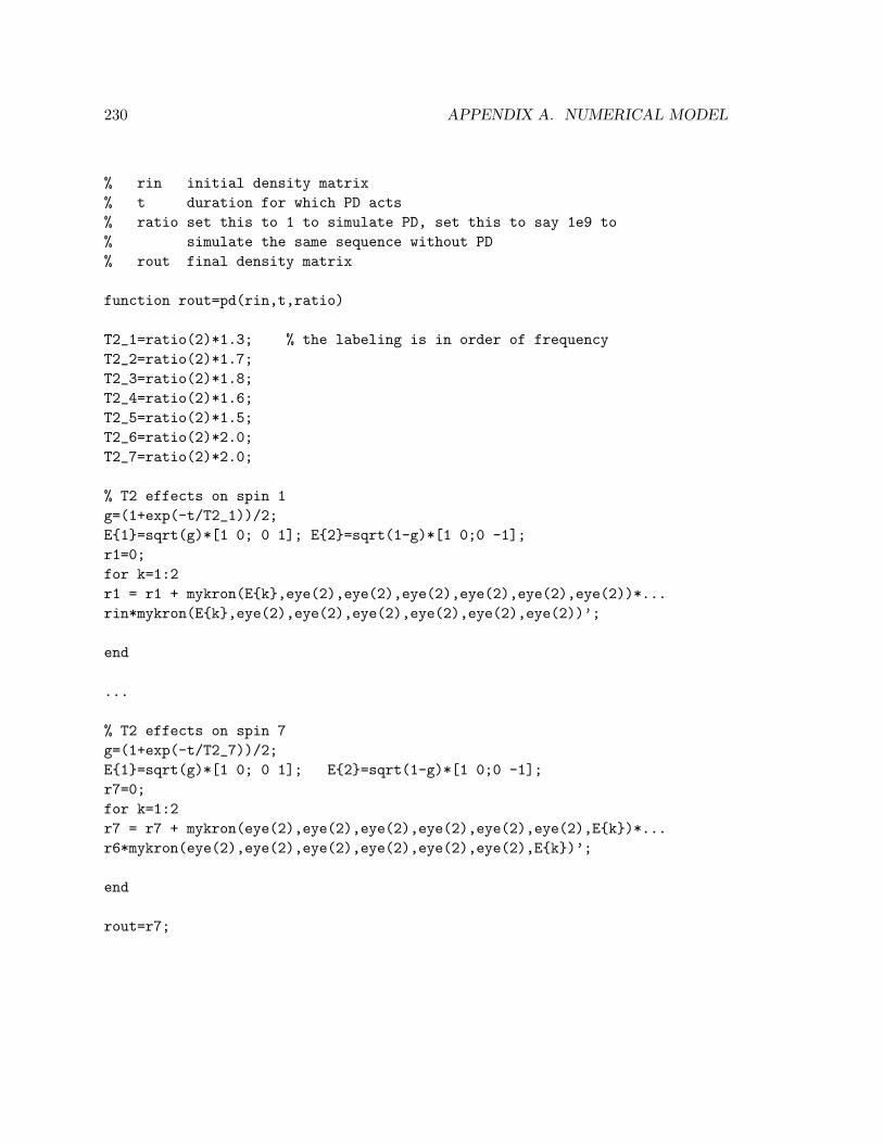
230 APPENDIX A. NUMERICAL MODEL
% rin initial density matrix% t duration for which PD acts% ratio set this to 1 to simulate PD, set this to say 1e9 to% simulate the same sequence without PD% rout final density matrix
function rout=pd(rin,t,ratio)
T2_1=ratio(2)*1.3; % the labeling is in order of frequencyT2_2=ratio(2)*1.7;T2_3=ratio(2)*1.8;T2_4=ratio(2)*1.6;T2_5=ratio(2)*1.5;T2_6=ratio(2)*2.0;T2_7=ratio(2)*2.0;
% T2 effects on spin 1g=(1+exp(-t/T2_1))/2;E1=sqrt(g)*[1 0; 0 1]; E2=sqrt(1-g)*[1 0;0 -1];r1=0;for k=1:2r1 = r1 + mykron(Ek,eye(2),eye(2),eye(2),eye(2),eye(2),eye(2))*...rin*mykron(Ek,eye(2),eye(2),eye(2),eye(2),eye(2),eye(2))’;
end
...
% T2 effects on spin 7g=(1+exp(-t/T2_7))/2;E1=sqrt(g)*[1 0; 0 1]; E2=sqrt(1-g)*[1 0;0 -1];r7=0;for k=1:2r7 = r7 + mykron(eye(2),eye(2),eye(2),eye(2),eye(2),eye(2),Ek)*...r6*mykron(eye(2),eye(2),eye(2),eye(2),eye(2),eye(2),Ek)’;
end
rout=r7;

A.7. HELPER PROGRAMS 231
A.7 Helper programs
% File: gop.m (generalized operator)% Date: 08-Oct-99% Author: Lieven Vandersypen <[email protected]>%% Usage: gop(s,U)% In: single-qubit unitary operator U, qubit name s% Out: n-spin unitary operator which acts on qubit s with U and% trivially on the remaining qubits
function gop=gop(s,U)
global nqubits
goplocal=U;
for position=1:(s-1)goplocal=kron(eye(2),goplocal);
endfor position=s+1:nqubits
goplocal=kron(goplocal,eye(2));endgop=goplocal;
% File: mykron.m% Date: 17-Aug-98% Author: I. Chuang <[email protected]>%% kronecker product function which accepts multiple arguments.
function out = mykron(ma,mb,varargin)
if (length(varargin) == 0)out = kron(ma,mb);return;
elseout = mykron(kron(ma,mb),varargin:);return;
end
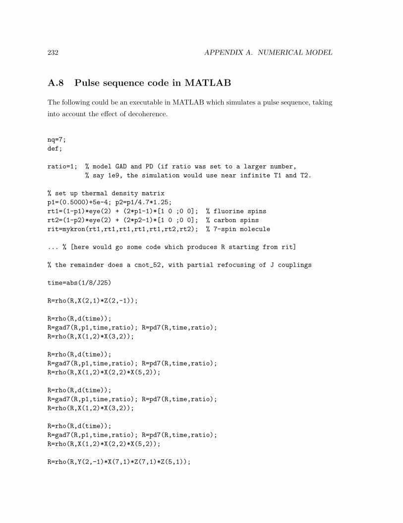
232 APPENDIX A. NUMERICAL MODEL
A.8 Pulse sequence code in MATLAB
The following could be an executable in MATLAB which simulates a pulse sequence, taking
into account the effect of decoherence.
nq=7;def;
ratio=1; % model GAD and PD (if ratio was set to a larger number,% say 1e9, the simulation would use near infinite T1 and T2.
% set up thermal density matrixp1=(0.5000)+5e-4; p2=p1/4.7*1.25;rt1=(1-p1)*eye(2) + (2*p1-1)*[1 0 ;0 0]; % fluorine spinsrt2=(1-p2)*eye(2) + (2*p2-1)*[1 0 ;0 0]; % carbon spinsrit=mykron(rt1,rt1,rt1,rt1,rt1,rt2,rt2); % 7-spin molecule
... % [here would go some code which produces R starting from rit]
% the remainder does a cnot_52, with partial refocusing of J couplings
time=abs(1/8/J25)
R=rho(R,X(2,1)*Z(2,-1));
R=rho(R,d(time));R=gad7(R,p1,time,ratio); R=pd7(R,time,ratio);R=rho(R,X(1,2)*X(3,2));
R=rho(R,d(time));R=gad7(R,p1,time,ratio); R=pd7(R,time,ratio);R=rho(R,X(1,2)*X(2,2)*X(5,2));
R=rho(R,d(time));R=gad7(R,p1,time,ratio); R=pd7(R,time,ratio);R=rho(R,X(1,2)*X(3,2));
R=rho(R,d(time));R=gad7(R,p1,time,ratio); R=pd7(R,time,ratio);R=rho(R,X(1,2)*X(2,2)*X(5,2));
R=rho(R,Y(2,-1)*X(7,1)*Z(7,1)*Z(5,1));

Appendix B
Pulse sequence three-spin Grover
search
We here give the final pulse sequences used in the experiment of Section 5.7. They are taken
from the C code submitted to the spectrometer, with additional comments for clarity.
======================================================================NOTATION======================================================================
Yb(1) represents a 1*pi/2 = pi/2 pulse on spin b about the Y axismXc(0.5) represents a 0.5*pi/2 = pi/4 pulse on spin c about the-X axis, etcetera
AB(), AC() and BC() represent simultaneous pulses on two spins. Thefirst two arguments are the tip angle in units of pi/2, and the lasttwo arguments are the phase of each pulse.
Example: AC(0.5,2,PHX,PHmY) performs a pi/4 pulse on spin a aboutthe X axis, and a pi pulse on spin c about the -Y axis
ABC() represents a simultaneous pulse on all three spins. The firstthree arguments are the tip angle in units of pi/2, and the lastthree arguments are the phase of each pulse.
=====================================================================OUTLINE=====================================================================
233

234 APPENDIX B. PULSE SEQUENCE THREE-SPIN GROVER SEARCH
delay(d1); /* THERMALIZATION */
tom3htemplab1(); /* TEMPORAL LABELING */
ABC(1,1,1,PHY,PHY,PHY); /* Hadamard on each spin */
/* the parameter ctype determines which will be the marked element x0that will be "found" during the execution of the algorithm */
pfa=2; pfb=2; pfc=2; /* default values */
if (ctype) /* if ctype=0, skip search */
if (((ctype-1)/4)%2) pfa=0;if (((ctype-1)/2)%2) pfb=0;if (((ctype-1)/1)%2) pfc=0;
loop(v9,v10); /* start loop Grover iterations *//* function evaluation */
ABC(pfa,pfb,pfc,PHX,PHX,PHX); /* depends on ctype */tom3hphaseflip4(); /* flip sign 111 term */ABC(pfa,pfb,pfc,PHmX,PHmX,PHmX); /* depends on ctype */
/* inversion about the average */ABC(1,1,1,PHY,PHY,PHY); /* pi/2 Y pulse on each spin */tom3hphaseflip4(); /* flip sign 111 term */ABC(1,1,1,PHmY,PHmY,PHmY); /* pi/2 -Y pulse on each spin */
endloop(v10);
/* close if (ctype) */
tomoPULSE; /* TOMOGRAPHY PULSES */
=====================================================================tom3hphaseflip4() - this function implements a diagonal unitary
operator with the elements [1 1 1 1 1 1 1 -1] on the diagonal=====================================================================
Yb(2); delay(1/8/Jbc); Xa(1); Ya(0.5); Xa(1); delay(1/8/Jbc);Yb(1); Xb(0.5); delay(1/4/Jab); mYc(2); delay(1/4/Jab); Yb(1); mXb(1);delay(1/8/Jbc); Ya(2); delay(1/8/Jbc);mXb(1); Yb(0.5); delay(1/4/Jab); Yc(1); Xc(0.5); Yc(1); delay(1/4/Jab);Yb(1); delay(1/8/Jac); mYb(2); delay(1/8/Jac);

235
=====================================================================tom3htemplab1() - this function implements one of several sequences,
each of which transforms the initial (thermal equilibrium) densitymatrix into one of the terms of the temporal labeling summation
=====================================================================
switch (ptype)case 0: break; /* I */case 1: /* cnotab */
Yb(1); delay(1/4/Jab); Xc(2); delay(1/4/Jab); BC(1,2,PHX,PHX);break;
case 2: /* cnotac */Yc(1); delay(1/4/Jac); Xb(2); delay(1/4/Jac); BC(2,1,PHX,PHX);break;
case 3: /* cnotbc, Jbc<0 */mYc(1); delay(1/4/Jbc); Xa(2); delay(1/4/Jbc); AC(2,1,PHX,PHX);break;
case 4: /* cnotba */Ya(1); delay(1/4/Jab); Xc(2); delay(1/4/Jab); AC(1,2,PHX,PHX);break;
case 5: /* cnotca */Ya(1); delay(1/4/Jac); Xb(2); delay(1/4/Jac); AB(1,2,PHX,PHX);break;
case 6: /* cnotcb, Jbc<0 */mYb(1); delay(1/4/Jbc); Xa(2); delay(1/4/Jbc); AB(2,1,PHX,PHX);break;
case 7: /* cnotab.cnotca (time -->) */Yb(1); delay(1/4/Jab); Xc(2); delay(1/4/Jab); BC(1,2,PHX,PHX);Ya(1); delay(1/4/Jac); Xb(2); delay(1/4/Jac); AB(1,2,PHX,PHX);break;

Bibliography
[ABO97] D. Aharonov and M. Ben-Or. Fault tolerant computation with constant error.
In Proceedings of the Twenty-Ninth Annual ACM Symposium on the Theory
of Computing, pp. 176–188, 1997.
[Abr61] A. Abragam. Principles of Nuclear Magnetism. Clarendon Press, Oxford,
1961.
[AGH+55] A.G. Anderson, R.L. Garwin, E.L. Hahn, J.W. Horton, G.L. Tucker, and R.M.
Walker. J. Appl. Physics, 26, 1324, 1955.
[AGR81] A. Aspect, P. Grangier, and G. Roger. Experimental tests of realistic local
theories via Bell’s theorem. Phys. Rev. Lett., 47(7), 460–463, 1981.
[AL97] D. S. Abrams and S. Lloyd. Simulation of many-body Fermi systems on a
quantum computer. Phys. Rev. Lett., 79(13), 2586–2589, 1997.
[AL99] D.S. Abrams and S. Lloyd. Quantum algorithm for providing exponential speed
increase for finding eigenvalues and eigenvectors. Phys. Rev. Lett., 83(24),
5162–5165, 1999.
[AV93] D. Abramovich and S. Vega. Derivation of broadband and narrowband excita-
tion pulses using the Floquet formalism. J. Magn. Reson. A, 105(18), 30–48,
1993.
[Ave00] D.V. Averin. Quantum computing and quantum measurement with mesoscopic
Josephson junctions. Fortschr. Phys., 48(9–11), 1055–1074, 2000.
[BB84] C. H. Bennett and G. Brassard. Quantum cryptography: Public key distri-
bution and coin tossing. In Proceedings of IEEE International Conference on
236
BIBLIOGRAPHY 237
Computers, Systems and Signal Processing, pp. 175–179, IEEE, New York,
1984. Bangalore, India, December 1984.
[BBBV97] C. H. Bennett, E. Bernstein, G. Brassard, and U. Vazirani. Strengths and
weaknesses of quantum computing. SIAM J. Comput., 26(5), 1510–1523, 1997.
[BBC+93] C. H. Bennett, G. Brassard, C. Crepeau, R. Jozsa, A. Peres, and W. Wootters.
Teleporting an unknown quantum state via dual classical and EPR channels.
Phys. Rev. Lett., 70, 1895–1899, 1993.
[BBC+95] A. Barenco, C. H. Bennett, R. Cleve, D. P. DiVincenzo, N. Margolus, P. Shor,
T. Sleator, J. Smolin, and H. Weinfurter. Elementary gates for quantum com-
putation. Phys. Rev. A, 52, 3457–3467, 1995.
[BBHT98] M. Boyer, G. Brassard, P. Høyer, and A. Tapp. Tight bounds on quantum
searching. Fortsch. Phys. – Prog. Phys., 46(4–5), 493–505, 1998.
[BBM+98] D. Boschi, S. Branca, F. De Martini, L. Hardy, and S. Popescu. Experimental
realization of teleporting an unknown pure quantum state via dual classical
and Einstein-Podolski-Rosen channels. Phys. Rev. Lett., 80, 1121–1125, 1998.
[BCDP96] D. Beckman, A. N. Chari, S. Devabhaktuni, and J. Preskill. Efficient networks
for quantum factoring. Phys. Rev. A, 54(2), 1034, 1996.
[BCHP96] J. Burdon, P.L. Coe, I.B. Haslock, and R.L. Powell. The hydrofluorocarbon
1,1,1,2-tetrafluoroethane (hfc-134a) as a ready source of trifluorovinyllithium.
J. Chem. Soc. Chem Commun., pp. 49–50, 1996.
[BCJ+99] S. L. Braunstein, C. M. Caves, R. Jozsa, N. Linden, S. Popescu, and R. Schack.
Separability of very noisy mixed states and implications for NMR quantum
computing. Phys. Rev. Lett., 83(5), 1054–1057, 1999.
[BCJD99] G. K. Brennen, C. M. Caves, P. S. Jessen, and I. H. Deutsch. Quantum logic
gates in optical lattices. Physical Review Letters, 82, 1060–1063, 1999.
[BD00] Charles H. Bennett and David P. DiVincenzo. Quantum information and
computation. Nature, 404, 247–55, 2000.

238 BIBLIOGRAPHY
[Bel64] John S. Bell. On the Einstein-Podolsy-Rosen paradox. Physics, 1, 195–200,
1964.
[Ben73] C. H. Bennett. Logical reversibility of computation. IBM J. Res. Dev., 17(6),
525–32, 1973.
[Ben80] P. Benioff. The computer as a physical system: A microscopic quantum me-
chanical Hamiltonian model of computers as represented by Turing machines.
J. Stat. Phys., 22(5), 563–591, 1980.
[Ben92] C. H. Bennett. Quantum cryptography using any two nonorthogonal states.
Phys. Rev. Lett., 68(21), 3121–3124, 1992.
[Ber84] M.V. Berry. Proc. R. Soc. London A, 392, 45, 1984.
[BFF+84] C.J. Bauer, R. Freeman, T. Frenkiel, J. Keeler, and A.J. Shaka. Gaussian
pulses. J. Magn. Reson., 58, 442–457, 1984.
[BHIW86] J. C. Bergquist, R. G. Hulet, W. M. Itano, and D. J. Wineland. Observation
of quantum jumps in a single atom. Phys. Rev. Lett., 57(14), 1699–1702, 1986.
[BHL+00] W. T. Buttler, R. J. Hughes, S. K. Lamoreaux, G. L. Morgan, J. E. Nordholt,
and C. G. Peterson. Daylight quantum key distribution over 1.6 km. Phys.
Rev. Lett., 84(24), 5652–5655, 2000.
[BHT98] G. Brassard, P. Høyer, and A. Tapp. Quantum counting. In Automata, Lan-
guages and Programming, 25th Int. Colloquium, Aalborg, Denmark, pp. 13–17,
Springer-Verlag, Berlin, 1998. arXive e-print quant-ph/9805082.
[BK98] S.L. Braunstein and H. J. Kimble. Teleportation of continuous quantum vari-
ables. Phys. Rev. Lett., 80, 869–72, 1998.
[BL00] S. Braunstein and H.-K. Lo, editors. Scalable Quantum Computers - paving
the way to realization. Wiley, Berlin, Germany, 2000. Reprint of Fortschr.
Phys., vol. 48(9-11), 2000. Special issue on the implementation of quantum
computers.
[Blo46] F. Bloch. Nuclear induction. Phys. Rev., 70(7-8), 460–474, 1946.
BIBLIOGRAPHY 239
[Blo49] N. Bloembergen. Physica, 15, 386, 1949.
[BMG+87] R. Bruschweiler, J.C. Madsen, C. Griesinger, O.W. Sørensen, and R.R. Ernst.
J. Magn. Reson., 73, 380, 1987.
[BPM+97] D. Bouwmeester, J. W. Pan, K. Mattle, M. Eibl, H. Weinfurter, and
A. Zeilinger. Experimental quantum teleportation. Nature, 390(6660), 575–
579, 1997.
[BS40] F. Bloch and A. Siegert. Magnetic resonance for nonrotating fields. Phys.
Rev., 57, 522–527, 1940.
[BSKM+96] M. Brune, F. Schmidt-Kaler, A. Maali, J. Dreyer, E. Hagley, J.-M. Raimond,
and S. Haroche. Quantum rabi oscillation: a direct test of field quantization
in a cavity. Phys. Rev. Lett., 76, 1800–1803, 1996.
[BW92] C. H. Bennett and S. J. Wiesner. Communication via one- and two-particle
operators on Einstein-Podolsky-Rosen states. Phys. Rev. Lett., 69, 2881–2884,
1992.
[CEMM98] R. Cleve, A. Ekert, C. Macchiavello, and M. Mosca. Quantum algorithms
revisited. Proc. R. Soc. London A, 454(1969), 339–354, 1998.
[CFH97] D. G. Cory, A. F. Fahmy, and T. F. Havel. Ensemble quantum computing by
NMR spectroscopy. Proc. Nat. Acad. Sci. USA, 94, 1634–1639, 1997.
[CGK98] I. L. Chuang, N. Gershenfeld, and M. Kubinec. Experimental implementation
of fast quantum searching. Phys. Rev. Lett., 18(15), 3408–3411, 1998.
[CGKL98] I. L. Chuang, N. Gershenfeld, M. G. Kubinec, and D. W. Leung. Bulk quantum
computation with nuclear-magnetic-resonance: theory and experiment. Proc.
R. Soc. London A, 454(1969), 447–467, 1998.
[Chu36] A. Church. An unsolvable problem of elementary number theory. Am. J.
Math., 58, 345, 1936.
[CKH+00] D. Collins, K.W. Kim, W.C. Holton, H. Sierzputowska-Gracz, and E.O. Ste-
jskal. NMR quantum computation with indirectly coupled gates. Phys. Rev.
A, 62, 022304, 2000.

240 BIBLIOGRAPHY
[CL95] I. L. Chuang and R. Laflamme. Quantum error correction by coding. arXive
e-print quant-ph/9511003, Oct 1995.
[Cle00] R. Cleve. The query complexity of order-finding. In Proceedings of the 15th
Annual IEEE Conference on Computational Complexity, Firenze, Italy, pp.
54–59, IEEE Computer Society Press, Los Alamitos, CA, 2000. arXive e-print
quant-ph/9911124.
[CLK+00] D.G. Cory, R. Laflamme, E. Knill, L. Viola, T.F. Havel, N. Boulant, G. Boutis,
E. Fortunato, S. Lloyd, R. Martinez, C. Negrevergne, M. Pravia, Y. Sharf,
G. Teklemariam, Y.S. Weinstein, and W.H. Zurek. NMR based quantum
information processing: achievements and prospects. Fortschr. Phys., 48(9–
11), 875–907, 2000.
[CMP+98] D. G. Cory, W. Mass, M. Price, E. Knill, R. Laflamme, W. H. Zurek, T. F.
Havel, and S. S. Somaroo. Experimental quantum error correction. Phys. Rev.
Lett., 81(10), 2152–2155, 1998.
[Cop94] D. Coppersmith. An approximate Fourier transform useful in quantum factor-
ing. IBM Research Report RC 19642, 1994.
[CPH98] D. G. Cory, M. D. Price, and T. F. Havel. Nuclear magnetic resonance spec-
troscopy: An experimentally accessible paradigm for quantum computing.
Physica D, 120, 82–101, 1998.
[CT91] T. M. Cover and J. A. Thomas. Elements of Information Theory. John Wiley
and Sons, New York, 1991.
[CTDL77] C. Cohen-Tannoudji, B. Diu, and F. Laloe. Quantum Mechanics (2 volumes).
John Wiley and Sons, New York, 1977.
[CVS01] D.E. Chang, L.M.K. Vandersypen, and M. Steffen. NMR implementation of
a building block for scalable quantum computation. Chem. Phys. Lett., 338,
337–344, 2001.
[CVZ+98] I. L. Chuang, L. M. K. Vandersypen, X. L. Zhou, D. W. Leung, and S. Lloyd.
Experimental realization of a quantum algorithm. Nature, 393(6681), 143–146,
1998.
BIBLIOGRAPHY 241
[CWK+01] B.E. Cole, J.B. Williams, B.T. King, M.S. Sherwin, and C.R. Stanley. Coherent
manipulation of semiconductor quantum bits with terahertz radiation. Nature,
410, 60–63, 2001.
[CZ95] J. I. Cirac and P. Zoller. Quantum computations with cold trapped ions. Phys.
Rev. Lett., 74, 4091, 1995.
[CZ00] J. I. Cirac and P. Zoller. A scalable quantum computer with ions in an array
of microtraps. Nature, 404, 579–581, 2000.
[DAK00] K. Dorai, Arvind, and A. Kumar. Implementing quantum-logic operations,
pseudopure state, and the Deutsch-Jozsa algorithm using non-commuting se-
lective pulses in NMR. Phys. Rev. A, 61, 042306(7), 2000.
[Dav65] M. D. Davis. The Undecidable. Raven Press, Hewlett, New York, 1965.
[DB00] I.H. Deutsch and G.K. Brennen. Quantum computing with neutral atoms in
an optical lattice. Fortschr. Phys., 48(9-11), 925–943, 2000.
[DBE95] D. Deutsch, A. Barenco, and A. Ekert. Universality in quantum computation.
Proc. R. Soc. London A, 449(1937), 669–677, 1995.
[DBIW89] F. Diedrich, J.C. Bergquist, W.M. Itano, and D.J. Wineland. Laser cooling to
the zero-point energy of motion. Phys. Rev. Lett., 62, 430, 1989.
[DBLW00] D.P. DiVincenzo, D.P. Bacon, D.A. Lidar, and K.B. Whaley. Universal quan-
tum computation with the exchange interactin. Nature, 408, 339, 2000.
[Deu85] D. Deutsch. Quantum theory, the Church-Turing Principle and the universal
quantum computer. Proc. R. Soc. Lond. A, 400, 97–117, 1985.
[Deu89] D. Deutsch. Quantum computational networks. Proc. R. Soc. London A, 425,
73, 1989.
[Die82] D. Dieks. Communication by EPR devices. Phys. Lett. A, 92(6), 271–272,
1982.
[DiV95a] D. P. DiVincenzo. Quantum computation. Science, 270, 255, 1995.
242 BIBLIOGRAPHY
[DiV95b] D. P. DiVincenzo. Two-bit gates are universal for quantum computation. Phys.
Rev. A, 51(2), 1015–1022, 1995.
[DiV98] D. P. DiVincenzo. Quantum gates and circuits. Proc. R. Soc. London A, 454,
261–276, 1998.
[DiV00] D. P. DiVincenzo. The physical implementation of quantum computers.
Fortschr. Physik, 48(9-11), 771–783, 2000.
[DJ92] D. Deutsch and R. Jozsa. Rapid solution of problems by quantum computation.
Proc. R. Soc. London A, 439, 553, 1992.
[DL99] D.P. DiVincenzo and D. Loss. Quantum computers and quantum coherence.
J. Magnetism and Magnetic Matls., 200, 202, 1999.
[dP79] M. Van der Puy. The reaction of molybdenum hexafluoride with carboxylic
acids. J. Fluor. Chem., 13, 375–378, 1979.
[EB90] L. Emsley and G. Bodenhausen. Phase shifts induced by transient bloch-siegert
effects in NMR. Chem. Phys. Lett., 168(3,4), 297–303, 1990.
[EBW87] R. R. Ernst, G. Bodenhausen, and A. Wokaun. Principles of Nuclear Magnetic
Resonance in One and Two Dimensions. Oxford University Press, Oxford,
1987.
[EJ96] A. Ekert and R. Jozsa. Quantum computation and Shor’s factoring algorithm.
Rev. Mod. Phys., 68, 1, 1996.
[EL75] J.W. Emsley and J.C. Lindon. NMR Spectroscopy using liquid crystal solvents.
Pergamon Press, Oxford, 1975.
[EM62] D.D. Elleman and S.L. Manatt. J. Chem. Phys., 36, 1945–1947, 1962.
[EM96] A. Ekert and C. Macchiavello. Error correction in quantum communication.
Phys. Rev. Lett., 77, 2585, 1996.
[EPR35] A. Einstein, B. Podolsky, and N. Rosen. Can quantum-mechanical description
of physical reality be considered complete? Phys. Rev., 47, 777–780, 1935.

BIBLIOGRAPHY 243
[Fey60] R.P. Feynman. There’s plenty of room at the bottom. In Engineer-
ing and Science, Caltech, Pasadena, CA, February 1960. Available at
http://www.zyvex.com/nanotech/feynman.html.
[Fey82] R. P. Feynman. Simulating physics with computers. Int. J. Theor. Phys., 21,
467, 1982.
[Fey85] R. P. Feynman. Quantum mechanical computers. Optics News, p. 11, February
1985.
[Fey96] Richard Feynman. Feynman Lectures on Computation. Addison-Wesley, New
York, 1996.
[FG59] G. Feher and E.A. Gere. Electron spin resonance experiments on donors in
silicon. ii. electron spin relaxation effects. Phys. Rev., 114, 1245–1256, 1959.
[FKR+99] R. Fiederling, M. Keim, G. Reuscher, W. Ossau, G. Schmidt, A. Waag, and
L.W. Molenkamp. Injection and detection of a spin-polarized current in a light
emitting diode. Nature, 402, 787–790, 1999.
[FLS65] R. P. Feynman, R. B. Leighton, and M. Sands. Volume III of The Feynman
Lectures on Physics. Addison-Wesley, Reading, Mass., 1965.
[FPC+00] J.R. Friedman, V. Patel, W. Chen, S.K. Tolpygo, and J.E. Lukens. Quantum
superposition of distinct macroscopic states. Nature, 406, 43–46, 2000.
[Fre97] R. Freeman. Spin Choreography. Spektrum, Oxford, 1997.
[Fre98] R. Freeman. Shaped radiofrequency pulses in high resolution NMR. Progr. in
NMR Spectr., 32, 59–106, 1998.
[FSH98] R.J. Fitzgerald, K.L. Sauer, and W. Happer. Chem. Phys. Lett., 284, 87, 1998.
[FT82] Edward Fredkin and Tommaso Toffoli. Conservative logic. Int. J. Theor. Phys.,
21(3/4), 219–253, 1982.
[FZF+00] X. Fang, X. Zhu, M. Feng, X. Mao, and F. Du. Experimental implementation
of dense coding using nuclear magnetic resonance. Phys. Rev. A, 61, 022307(5),
2000.

244 BIBLIOGRAPHY
[GC97] N. Gershenfeld and I. L. Chuang. Bulk spin resonance quantum computation.
Science, 275, 350–356, 1997.
[GC98] N. Gershenfeld and I.L. Chuang. Quantum computing with molecules. Scien-
tific American, June 1998.
[GC99] D. Gottesman and I. L. Chuang. Quantum teleportation is a universal com-
putational primitive. Nature, 402, 390–392, 1999.
[GF91] H. Geen and R. Freeman. Band-selective radiofrequency pulses. J. Magn.
Reson., 93, 93–141, 1991.
[GG99] J.-M. Gerard and B. Gayral. In H. Benisty, J.-M. Gerard, and C. Weisbuch, ed-
itors, QED phenomena and applications of microcavities and photonic crystals,
Springer-Verlag, Berlin, 1999.
[GMS68] M. Green, N. Mayne, and F.G.A. Stone. J. Chem. Soc. (A), p. 902, 1968.
[Got98] D. Gottesman. Theory of fault-tolerant quantum computation. Phys. Rev. A,
57(1), 127–137, 1998.
[Gro96] Lov K. Grover. A fast quantum mechanical algorithm for database search.
In 28th ACM Symposium on Theory of Computation, p. 212, Association for
Computing Machinery, New York, 1996.
[Gro97] Lov K. Grover. Quantum mechanics helps in searching for a needle in a
haystack. Phys. Rev. Lett., 79(2), 325, 1997.
[GRTZ01] N. Gisin, G. Ribordy, W. Tittel, and H. Zbinden. Quantum cryptography.
arXive e-print quant-ph/0101098, 2001.
[GS01] B. Georgeot and D.L. Shepelyanky. Exponential gain in quantum computing
of quantum chaos and localization. Phys. Rev. Lett., 86(13), 2890–2893, 2001.
[HBG00] P. Hubler, J. Bargon, and S.J. Glaser. Nuclear magnetic resonance quantum
computing exploiting the pure spin state of para hydrogen. J. Chem. Phys.,
113(6), 2056–2059, 2000.
BIBLIOGRAPHY 245
[HHK+98] S. E. Hamann, D. L. Haycock, G. Klose, P. H. Pax, I. H. Deutsch, and P. S.
Jessen. Resolved-sideband raman cooling to the ground state of an optical
lattice. Phys. Rev. Lett., 80, 4149–4152, 1998.
[HMM90] X. Hao, J.S. Moodera, and R. Meservey. Spin-filter effect of ferromagnetic
europium sulfide tunnel barriers. Phys. Rev. B, 42(13), 8235–8243, 1990.
[HR76] D.I. Hoult and R.E. Richards. The signal-to-noise ratio of the nuclear magnetic
resonance experiment. J. Magn. Reson., 24, 71–85, 1976.
[HU79] J.E. Hopcroft and J.D. Ullman. Introduction to automata theory, languages,
and computation. Addison-Wesley, Reading, MA, 1979.
[HW60] G. H. Hardy and E. M. Wright. An Introduction to the Theory of Numbers,
Fourth Edition. Oxford University Press, London, 1960.
[IAB+99] A. Imamoglu, D. D. Awschalom, G. Burkard, D. P. DiVincenzo, D. Loss,
M. Sherwin, and A. Small. Quantum information processing using quantum
dot spins and cavity qed. Phys. Rev. Lett., 83(20), 4204–7, 1999.
[Jee82] J. Jeener. Superoperators in magnetic resonance. Adv. Magn. Res., 10, 1–51,
1982.
[Jef63] C.D. Jeffries. Dynamic nuclear orientation. Wiley, New York, 1963.
[JK99] J. A. Jones and E. Knill. Efficient refocussing of one spin and two spin inter-
actions for NMR quantum computation. J. Magn. Reson., 141, 322, 1999.
[JKB+87] W.R. Dolbier Jr., H. Koroniak, D.J. Burton, P.L. Heinze, A.R. Bailey, G.S.
Shaw, and S.W. Hansen. Kinetic and thermodynamic studies of the thermal
electrocyclic interconversions of perfluorinated dienes an cyclobutenes. J. Am.
Chem. Soc., 109, 219–225, 1987.
[JM98] J. A. Jones and M. Mosca. Implementation of a quantum algorithm to solve
Deutsch’s problem on a nuclear magnetic resonance quantum computer. J.
Chem. Phys., 109, 1648, 1998.
[JM99] J.A. Jones and M. Mosca. Approximate quantum counting on an NMR en-
semble quantum computer. Phys. Rev. Lett., 83, 1050, 1999.
246 BIBLIOGRAPHY
[JMH98] J. A. Jones, M. Mosca, and R. H. Hansen. Implementation of a quantum
search algorithm on a nuclear magnetic resonance quantum computer. Nature,
393(6683), 344, 1998.
[Jon01] J.A. Jones. NMR quantum computation. Progr. NMR Spectr., 38, 325–360,
2001.
[KA98] J.M. Kikkawa and D.D. Awschalom. Phys. Rev. Lett., 80, 4313, 1998.
[Kan98] Bruce Kane. A silicon-based nuclear spin quantum computer. Nature, 393,
133–137, 1998.
[KCL98] E. Knill, I. Chuang, and R. Laflamme. Effective pure states for bulk quantum
computation. Phys. Rev. A, 57(5), 3348–3363, 1998.
[KF95] E. Kupce and R. Freeman. Close encounters between soft pulses. J. Magn.
Reson. A, 112, 261–264, 1995.
[Kit95] A. Yu. Kitaev. Quantum measurements and the Abelian stabilizer problem.
arXive e-print quant-ph/9511026, 1995.
[Kit97] A. Y. Kitaev. Quantum computations: algorithms and error correction. Russ.
Math. Surv., 52(6), 1191–1249, 1997.
[KL96] E. Knill and R. Laflamme. A theory of quantum error correcting codes. Phys.
Rev. A, 55(2), 900–911, 1996.
[KL98] E. Knill and R. Laflamme. On the power of one bit of quantum information.
Phys. Rev. Lett., 81, 5672–5675, 1998.
[KLL00] H. Kim, J.-S. Lee, and S. Lee. Implementation of the refined deutsch-jozsa
algorithm on a three-bit NMR quantum computer. Phys. Rev. A, 62, 022312,
2000.
[KLM01] E. Knill, R. Laflamme, and G. J. Milburn. A scheme for efficient quantum
computation with linear optics. Nature, 409, 46–52, 2001.
[KLMN01] E. Knill, R. Laflamme, R. Martinez, and C. Negrevergne. Implementation of
the five-qubit error correction benchmark. arXiv:quant-ph/0101034, 2001.
BIBLIOGRAPHY 247
[KLMT00] E. Knill, R. Laflamme, R. Martinez, and C.-H. Tseng. An algorithmic bench-
mark for quantum information processing. Nature, 404, 368–370, 2000.
[KLZ98] E. Knill, R. Laflamme, and W. H. Zurek. Resilient quantum computation.
Science, 279(5349), 342–345, 1998.
[Knu98] D. E. Knuth. Seminumerical Algorithms 3rd Edition, Volume 2 of The Art of
Computer Programming. Addison-Wesley, Reading, Massachusetts, 1998.
[Kob94] N. Koblitz. A Course in Number Theory and Cryptography. Springer-Verlag,
New York, 1994.
[Kra83] Karl Kraus. States, Effects, and Operations: Fundamental Notions of Quantum
Theory. Lecture Notes in Physics, Vol. 190. Springer-Verlag, Berlin, 1983.
[KSF01] A. Khitrin, H. Sun, and B.M. Fung. Method of multifrequency excitation for
creating pseudopure states for NMR quantum computing. Phys. Rev. A, 63,
020301(4), 2001.
[KWM+98] B. E. King, C. S. Wood, C. J. Myatt, Q. A. Turchette, D. Leibfried, W. M.
Itano, C. Monroe, and D. J. Wineland. Cooling the collective motion of trapped
ions to initialize a quantum register. Phys. Rev. Lett., 81, 1525–1529, 1998.
[Lan61] R. Landauer. Irreversibility and heat generation in the computing process.
IBM J. Res. Dev., 5, 183, 1961.
[LB99] S. Lloyd and S. Braunstein. Quantum computation over continuous variables.
Phys. Rev. Lett., 82, 1784–1787, 1999.
[LBCF99] N. Linden, H. Barjat, R.J. Carbajo, and R. Freeman. Pulse sequences for
NMR quantum computers: how to manipulate nuclear spins while freezing the
motion of coupled neighbours. Chem. Phys. Lett., 305, 28–34, 1999.
[LBF98] N. Linden, H. Barjat, and R. Freeman. Am implementation of the deutsch-
jozsa algorithm on a three-qubit NMR quantum computer. Chem. Phys. Lett,
296, 61–67, 1998.
[LCW+96] C. Livermore, C.H. Crouch, R.M. Westervelt, K.L. Campman, and A.C. Gos-
sard. The Coulomb blockade in coupled quantum dots. Science, 274, 1332–
1335, 1996.
248 BIBLIOGRAPHY
[LCYY00] D. W. Leung, I. L. Chuang, F. Yamaguchi, and Y. Yamamoto. Efficient im-
plementation of coupled logic gates for quantum computation. Phys. Rev. A,
61, 042310(7), 2000.
[LD98] Daniel Loss and David P. DiVincenzo. Quantum computation with quantum
dots. Phys. Rev. A, 57, 120–126, 1998.
[Lec63] Y. Lecerf. Machines de Turing reversibles. Comptes Rendus, 257, 2597–2600,
1963.
[Lev01] J. Levy. Universal quantum computation with spin-1/2 pairs and heisenberg
exchange. arXive e-print quant-ph/0101057, 2001.
[LFF82] M.H. Levitt, R. Freeman, and T. Frenkiel. J. Magn. Reson., 47, 328, 1982.
[LGD+00] T.D. Ladd, J.R. Goldman, A. Dana, F. Yamaguchi, and Y. Yamamoto. Quan-
tum computation in a one-dimensional crystal lattice with NMR force mi-
croscopy. arXive e-print quant-ph/0009122, 2000.
[LK97] C.K. Law and H.J. Kimble. Deterministic generation of a bit-stream of single-
photon pulses. J. Mod. Optics, 44, 2067, 1997.
[LKF99] N. Linden, E. Kupce, and R. Freeman. NMR quantum logic gates for homonu-
clear spin systems. Chem. Phys. Lett, 311, 321–327, 1999.
[LKZ+98] R. Laflamme, E. Knill, W. H. Zurek, P. Catasti, and S. V. S. Mariappan. NMR
GHZ. Phil. Trans. Roy. Soc. Lond. A, 356, 1941–1948, 1998.
[Llo93] Seth Lloyd. A potentially realizable quantum computer. Science, 261, 1569,
1993.
[Llo95a] S. Lloyd. Almost any quantum logic gate is universal. Phys. Rev. Lett., 75(2),
346–349, 1995.
[Llo95b] Seth Lloyd. Quantum-mechanical computers. Scientific American, 273(4), 44,
October 1995.
[Llo96] S. Lloyd. Universal quantum simulators. Science, 273, 1073, 1996.

BIBLIOGRAPHY 249
[LMPZ96] R. Laflamme, C. Miquel, J.-P. Paz, and W. H. Zurek. Perfect quantum error
correction code. Phys. Rev. Lett., 77, 198, 1996.
[LVZ+99] D. Leung, L. Vandersypen, X. Zhou, M. Sherwood, C. Yannoni, and I. Chuang.
Experimental realization of a two-bit phase damping quantum code. Phys. Rev.
A, 60(3), 1924–1943, 1999.
[MCK00] M. Marjanska, I.L. Chuang, and M.G. Kubinec. J. Chem. Phys., 112, 5095,
2000.
[ME61] J.F. Maher and D.F. Evans. Proc. Chem. Soc., pp. 208–209, June 1961.
[Meh83] M. Mehring. High resolution NMR in solids. Spring-Verlag, Berlin, 1983.
[Mer85] N. D. Mermin. Is the moon there when nobody looks? Reality and the quantum
theory. Physics Today, p. 45, April 1985.
[MFM+00] R. Marx, A.F. Fahmy, J.M. Myers, W. Bermel, and S.J. Glaser. Approaching
five-bit NMR quantum computing. Phys. Rev. A, 62, 123310–8, 2000.
[MHN+97] X. Maıtre, E. Hagley, G. Nogues, C. Wunderlich, P. Goy, M. Brune, J.-M.
Raimond, and S. Haroche. Quantum memory with a single photon in a cavity.
Phys. Rev. Lett., 79, 769–772, 1997.
[Mil89] G. J. Milburn. Quantum optical fredkin gate. Phys. Rev. Lett., 62(18), 2124–
2127, 1989.
[MKA+00] I. Malajovich, J. M. Kikkawa, D. D. Awschalom, J. J. Berry, and N. Samarth.
Coherent transfer of spin through a semiconductor heterointerface. Phys. Rev.
Lett., 84(5), 2000.
[MMK+95] C. Monroe, D. M. Meekhof, B. E. King, W. M. Itano, and D. J. Wineland.
Demonstration of a fundamental quantum logic gate. Phys. Rev. Lett., 75,
4714, 1995.
[MOL+99] J. E. Mooij, T. P. Orlando, L. Levitov, Lin Tian, Caspar H. van der Waal,
and Seth Lloyd. Josephson persistent-current qubit. Science, 285, 1036–1039,
1999.

250 BIBLIOGRAPHY
[MPZ00] C. Macchiavello, G.M. Palma, and A. Zeilinger, editors. Quantum computation
and quantum information theory. World Scientific, Singapore, 2000.
[MS99] K. Mølmer and A. Sørensen. Multiparticle entanglement of hot trapped ions.
Phys. Rev. Lett., 82, 1835–1838, 1999.
[MSS99] Y. Maklin, Gerd Schon, and Alexander Shnirman. Josephson-junction qubits
with controlled couplings. Nature, 398, 305–307, 1999.
[MTCK96] H. Mabuchi, Q.A. Turchette, M.S. Chapman, and H.J. Kimble. Real-time
detection of individual atoms falling through a high finesse optical cavity. Opt.
Lett., 21, 1393–1395, 1996.
[MZG96] A. Muller, H. Zbinden, and N. Gisin. Quantum cryptography over 23 km in
installed under-lake telecom fibre. Europhys. Lett., 33, 334–339, 1996.
[NC00] M.A. Nielsen and I.L. Chuang. Quantum computation and quantum informa-
tion. Cambridge University Press, Cambridge, England, 2000.
[NCL00] R.J. Nelson, D.G. Cory, and S. Lloyd. Experimental demonstration of
Greenberger-Horne-Zeilinger correlations using nuclear magnetic resonance.
Phys. Rev. A, 61, 022106(5), 2000.
[NCT97] Y. Nakamura, C.D. Chen, and J.S. Tsai. Spectroscopy of energy-level splitting
between two macroscopic quantum states of charge coherently superposed by
josephson coupling. Phys. Rev. Lett., 79, 2328–2331, 1997.
[NKL98] M. A. Nielsen, E. Knill, and R. Laflamme. Complete quantum teleportation
using nuclear magnetic resonance. Nature, 396(6706), 52–55, 1998.
[NPT99] Y. Nakamura, Yu. A. Pashkin, and J. S. Tsai. Coherent control of macroscopic
quantum states in a single-cooper-pair box. Nature, 398, 786–788, 1999.
[NRO+99] G. Nogues, A. Rauschenbeutel, S. Osnaghi, M. Brune, J. M. Raimond, and
S. Haroche. Seeing a single photon without destroying it. Nature, 400, 239–
242, 1999.
[NSD86] W. Nagourney, J. Sandberg, and H. Dehmelt. Shelved optical electron am-
plifier: observation of quantum jumps. Phys. Rev. Lett., 56(26), 2797–2799,
1986.
BIBLIOGRAPHY 251
[OOC+91] J.-M. Ouvrard, B. N. Ouvrard, J. Courtieu, C. L. Mayne, and D. M. Grant.
J. Magn. Reson., 93, 225, 1991.
[OSS+01] J.L. O’Brien, S.R. Schofield, M.Y. Simmons, R.G. Clark, A.S. Dzurak, N.J.
Curson, B.E. Kane, N. S. McAlpine, M.E. Hawley, and G.W. Brown. Towards
the fabrication of phosphorous qubits for a silicon quantum computer. To
appear in Phys. Rev. B, 2001.
[OYB+99] Y. Ohno, D.K. Young, B. Beschoten, F. Masukura, H. Ohno, and D.D.
Awschalom. Electrical spin injection in a ferromagnetic semiconductor het-
erostructure. Nature, 402, 790–792, 1999.
[Pap94] C. M. Papadimitriou. Computational Complexity. Addison-Wesley, Reading,
Massachusetts, 1994.
[Pat91] S.L. Patt. Single- and multiple-frequency-shifted laminar pulses. J. Magn.
Reson., 96, 94–102, 1991.
[PD99] P. M. Platzman and M. I. Dykman. Quantum computing with electrons float-
ing on liquid helium. Science, 284, 1967, 1999.
[Per93] A. Peres. Quantum Theory: Concepts and Methods. Kluwer Academic, Dor-
drecht, 1993.
[PRN91] J. Pauly, P. Le Roux, and Dwight Nishimura. Parameter relations for the
Shinnar-Le Roux selective excitation pulse design algorithm. IEEE Transac-
tions on medical imaging, 10(1), 53–65, 1991.
[PRS00] P.Grangier, G. Reymond, and N. Schlosser. Implementations of quantum com-
puting using cavity quantum electrodynamics schemes. Fortschr. Phys., 48(9-
11), 859–874, 2000.
[Red57] A.G. Redfield. IBM J. Res. Dev., 1, 19, 1957.
[Red65] A.G. Redfield. Adv. Magn. Res., 1, 1–32, 1965.
[RGR+01] H. Rohde, S. T. Gulde, C. F. Roos, P. A. Barton, D. Leibfried, J. Eschner,
F. Schmidt-Kaler, and R. Blatt. Sympathetic ground state cooling and coher-
ent manipulation with two-ion-crystals. J. Opt. B, 3, S34, 2001.

252 BIBLIOGRAPHY
[RLM+00] C. F. Roos, D. Leibfried, A. Mundt, F. Schmidt-Kaler, J. Eschner, and
R. Blatt. Experimental demonstration of ground state laser cooling with elec-
tromagnetically induced transparency. Phys. Rev. Lett., 85(26), 5547–5550,
2000.
[RNO+00] A. Rauschenbeutel, G. Nogues, S. Osnaghi, P. Bertet, M. Brune, J.-M. Rai-
mond, and Serge Haroche. Step-by-step engineered multiparticle entanglement.
Science, 288, 2024–2028, 2000.
[RSA78] R. L. Rivest, A. Shamir, and L. M. Adleman. A method of obtaining digital
signatures and public-key cryptosystems. Comm. ACM, 21(2), 120–126, 1978.
[RYS92] D. Rugar, C.S. Yannoni, and J.A. Sidles. Mechanical detection of magnetic
resonance. Nature, 360, 563, 1992.
[Sak95] J. J. Sakurai. Modern Quantum Mechanics. Addison-Wesley, Reading, Mass.,
1995.
[SC99] R. Schack and C. M. Caves. Classical model for bulk-ensemble NMR quantum
computation. Phys. Rev. A, 60(6), 4354–4362, 1999.
[Sch35] Erwin Schrodinger. Die gegenwartage Situation in der Quantenmechanik. Die
Naturwissenschaften, 23, 807–812, 824–828, 844–849, 1935.
[SCS+00] Y. Sharf, D.G. Cory, S.S. Somaroo, T.F. Havel, E. Knill, and R. Laflamme. A
study of quantum error correction by geometric algebra and liquid-state NMR
spectroscopy. Molec. Phys., 98(17), 1347–1363, 2000.
[SEP67] A. Saupe, G. Englert, and A. Povh. ACS Adv. in Chem. Ser., 63, 51, 1967.
[SHC00] Y. Sharf, T.F. Havel, and D.G. Cory. Spatially encoded pseudopure states for
NMR quantum-information processing. Phys. Rev. A, 62, 052314(8), 2000.
[Sho94] P. W. Shor. Algorithms for quantum computation: discrete logarithms and fac-
toring. In Proceedings, 35th Annual Symposium on Foundations of Computer
Science, pp. 124–134, IEEE Press, Los Alamitos, CA, 1994.
[Sho95] P. W. Shor. Scheme for reducing decoherence in quantum memory. Phys. Rev.
A, 52, 2493, 1995.

BIBLIOGRAPHY 253
[Sho97] P. W. Shor. Polynomial-time algorithms for prime factorization and discrete
logarithms on a quantum computer. SIAM J. Comp., 26(5), 1484–1509, 1997.
[Sim94] D. Simon. On the power of quantum computation. In Proceedings, 35th Annual
Symposium on Foundations of Computer Science, pp. 116–123, IEEE Press,
Los Alamitos, CA, 1994.
[Sim97] D. R. Simon. On the power of quantum computation. SIAM J. Comput.,
26(5), 1474–1483, 1997.
[SKK+00] C.A. Sackett, D. Kielpinsky, B.E. King, C. Langer, V. Meyer, C.J. Myatt,
M. Rowe, Q.A. Turchette, W.M. Itano, D.J. Wineland, and C. Monroe. Ex-
perimental entanglement of four particles. Nature, 404, 256–258, 2000.
[Sli96] Charles P. Slichter. Principles of Magnetic Resonance. Springer, Berlin, 1996.
[SMY+01] B.C. Stipe, H.J. Mamin, C.S. Yannoni, T.D. Stowe, T.W. Kenny, and D. Ru-
gar. Electron spin relaxation induced by a micron-sized ferromagnet. in prepa-
ration for submission to Science, 2001.
[SN96] B. W. Schumacher and M. A. Nielsen. Quantum data processing and error
correction. Phys. Rev. A, 54(4), 2629, 1996.
[SOF94] U. Sakaguchi, H. Ozawa, and T. Fukumi. Method for effective pure states with
any number of spins. Phys. Rev. A, 61, 042313(5), 1994.
[SPM86] D. Suter, A. Pines, and M. Mehring. Indirect phase detection of NMR spinor
transitions. Phys. Rev. Lett., 57, 242–244, 1986.
[Ste96] A. M. Steane. Error correcting codes in quantum theory. Phys. Rev. Lett., 77,
793, 1996.
[Ste98] A. Steane. Quantum computing. Rep. Prog. Phys., 61(2), 117–173, 1998.
[STH+99] S. Somaroo, C. H. Tseng, T. F. Havel, R. Laflamme, and D. G. Cory. Quantum
simulations on a quantum computer. Phys. Rev. Lett., 82, 5381–5384, 1999.
[SV99] L. J. Schulman and U. Vazirani. Molecular scale heat engines and scalable
quantum computation. Proc. 31st Ann. ACM Symp. on Theory of Computing
(STOC ’99), pp. 322–329, 1999.
254 BIBLIOGRAPHY
[SVC00] M. Steffen, L.M.K. Vandersypen, and I.L. Chuang. Simultaneous soft pulses
applied at nearby frequencies. J. Magn. Reson., 146, 369–374, 2000.
[SVC01] M. Steffen, L.M.K. Vandersypen, and I.L. Chuang. Toward quantum com-
putation: a five-qubit quantum processor. IEEE Micro, 21(2), 24–34, March
2001.
[TAH+96] S. Tarucha, D.G. Austing, T. Honda, R.J. van der Hage, and L. P. Kouwen-
hoven. Phys. Rev. Lett., 77, 3613, 1996.
[Tap98] A. Tapp. unpublished, 1998.
[THL+95] Q. A. Turchette, C. J. Hood, W. Lange, H. Mabuchi, and H. J. Kimble. Mea-
surement of conditional phase shifts for quantum logic. Phys. Rev. Lett., 75,
4710, 1995.
[TM73] P.M. Tedrow and R. Meservey. Spin polarization of electrons tunneling from
films of Fe, Co, Ni and Ga. Phys. Rev. B, 7(1), 318–326, 1973.
[Tof80] T. Toffoli. Reversible computing. In W. de Bakker and J. van Leeuwen,
editors, Automata, Languages, and Programming, pp. 632–644. Springer, New
York, 1980.
[TSS+99] D.H. Tseng, S. Somaroo, Y. Sharf, E. Knill, R. Laflamme, T.F. Havel, and
D.G. Cory. Quantum simulation of a three-body-interaction hamiltonian on
an NMR quantum computer. Phys. Rev. A, 61, 012302(6), 1999.
[Tur36] A. M. Turing. On computable numbers, with an application to the Entschei-
dungsproblem. Proc. Lond. Math. Soc. 2 (reprinted in [Dav65]), 42, 230, 1936.
[TWK+98] Q.A. Turchette, C.S. Wood, B.E. King, C.J. Myatt, D. Leibfried, W.M. Itano,
C. Monroe, and D.J. Wineland. Deterministic entanglement of two trapped
ions. Phys. Rev. Lett., 81, 3631–3634, 1998.
[Unr95] W. G. Unruh. Maintaining coherence in quantum computers. Phys. Rev. A,
51(2), 992–997, 1995.
[VLV+01] A.S. Verhulst, O. Liivak, H.M. Vieth, C.S. Yannoni, and I.L. Chuang. Non-
thermal nuclear magnetic resonance quantum computing using hyperpolarized
xenon. submitted to Appl. Phys. Lett., 2001.

BIBLIOGRAPHY 255
[VSB+00] L.M.K. Vandersypen, M. Steffen, G. Breyta, C.S. Yannoni, R. Cleve, and I. L.
Chuang. Experimental realization of an order-finding algorithm with an NMR
quantum computer. Phys. Rev. Lett., 85(25), 5452–5455, 2000.
[VSB+01] L.M.K. Vandersypen, M. Steffen, G. Breyta, C.S. Yannoni, R. Cleve, and
I. L. Chuang. Experimental realization of shor’s quantum factoring algorithm
(15 = 3× 5). in preparation, 2001.
[VSS+00] L.M.K. Vandersypen, M. Steffen, M. H. Sherwood, C.S. Yannoni, G. Breyta,
and I. L. Chuang. Implementation of a three-quantum-bit search algorithm.
Appl. Phys. Lett., 76(5), 646–648, 2000.
[vtW+00] C.H. van der Wal, A.C.J. ter Haar, F.K. Wilhelm, R.N. Schouten, C.J.P.M.
Harmans, T.P. Orlando, S. Lloyd, and J.E. Mooij. Quantum superposition of
macroscopic persistent-current states. Science, 290, 773–777, 2000.
[VV78] R.L. Vold and R.R. Vold. Nuclear magnetic relaxation in coupled spin systems.
Progr. in NMR Spectr., 12, 79–133, 1978.
[VYC01] L.M.K. Vandersypen, C.S. Yannoni, and I.L. Chuang. Liquid state NMR quan-
tum computing. In D.M. Grant and R.K. Harris, editors, to appear in The en-
cyclopedia of NMR (supplement). John Wiley and Sons, West Sussex, England,
2001.
[VYSC99] L. M. K. Vandersypen, C. S. Yannoni, M. H. Sherwood, and I. L. Chuang.
Realization of effective pure states for bulk quantum computation. Phys. Rev.
Lett., 83, 3085–3088, 1999.
[VYW+99] Rutger Vrijen, Eli Yablonovitch, Kang Wang, Hong Wen Jiang, Alex Balandin,
Vwani Roychowdhury, Tal Mor, and David DiVincenzo. Electron spin reso-
nance transistors for quantum computing in silicon-germanium heterostruc-
tures. arXive e-print quant-ph/9905096, 1999.
[War84] W. Warren. Effects of arbitrary laser or NMR pulse shapes on population
inversion and coherence. J. Chem. Phys., 81(12), 5437–5448, 1984.

256 BIBLIOGRAPHY
[WMI+98] D. J. Wineland, C. Monroe, W. M. Itano, D. Leibfried, B. E. King, and
D. M. Meekhof. Experimental issues in coherent quantum-state manipulation
of trapped atomic ions. J. Res. Natl. Inst. Stand. Tech., 103, 259, 1998.
[WPF+01] Y.S. Weinstein, M.A. Pravia, E.M. Fortunato, S. Lloyd, and D.G. Cory. Im-
plementation of the quantum fourier transform. Phys. Rev. Lett., 86(9), 1889–
1891, 2001.
[WZ82] W. K. Wootters and W. H. Zurek. A single quantum cannot be cloned. Nature,
299, 802–803, 1982.
[Yao93] A. C. Yao. Quantum circuit complexity. Proc. of the 34th Ann. IEEE Symp.
on Foundations of Computer Science, pp. 352–361, 1993.
[YSV+99] C.S. Yannoni, M.H. Sherwood, L.M.K. Vandersypen, M.G. Kubinec, D.C.
Miller, and I.L. Chuang. Nuclear magnetic resonance quantum computing
using liquid crystal solvents. Appl. Phys. Lett., 75(22), 3563–3565, 1999.
[YY99] F. Yamaguchi and Y. Yamamoto. Crystal lattice quantum computer. Appl.
Phys. A, 68, 1–8, 1999.
[Zur82] W. H. Zurek. Environment-induced super-selection rules. Phys. Rev. D, 26(8),
1862–1880, 1982.
[Zur91] W. H. Zurek. Decoherence and the transition from quantum to classical. Phys.
Today, 44(10), 36–44, 1991.