UNIVERSITY OF CALIFORNIA, SAN DIEGO

Experimental Studies of Multi-Species Pure Ion Plasmas: CyclotronModes, Long-Range Collisional Drag, and Non-Linear Langmuir Waves

A dissertation submitted in partial satisfaction of the

requirements for the degree

Doctor of Philosophy

in

Physics

by

Matthew Affolter

Committee in charge:

Professor C. Fred Driscoll, ChairProfessor Robert E. ContinettiProfessor Daniel H. E. DubinProfessor Clifford M. SurkoProfessor George R. Tynan

2016

Copyright

Matthew Affolter, 2016

All rights reserved.

The dissertation of Matthew Affolter is approved, and

it is acceptable in quality and form for publication on

microfilm and electronically:

Chair

University of California, San Diego

2016

iii

DEDICATION

To my parents, Bob and Mandy, and my grandfather, Frank Wilson,

for the many years of support and encouragement.

iv

EPIGRAPH

The desire for knowledge shapes a man.

—Patrick Rothfuss, The Wise Man’s Fear

v

TABLE OF CONTENTS

Signature Page . . . . . . . . . . . . . . . . . . . . . . . . . . . . . . . . . . . iii

Dedication . . . . . . . . . . . . . . . . . . . . . . . . . . . . . . . . . . . . . . iv

Epigraph . . . . . . . . . . . . . . . . . . . . . . . . . . . . . . . . . . . . . . v

Table of Contents . . . . . . . . . . . . . . . . . . . . . . . . . . . . . . . . . . vi

List of Figures . . . . . . . . . . . . . . . . . . . . . . . . . . . . . . . . . . . viii

List of Tables . . . . . . . . . . . . . . . . . . . . . . . . . . . . . . . . . . . . ix

Acknowledgements . . . . . . . . . . . . . . . . . . . . . . . . . . . . . . . . . x

Vita . . . . . . . . . . . . . . . . . . . . . . . . . . . . . . . . . . . . . . . . . xii

Abstract of the Dissertation . . . . . . . . . . . . . . . . . . . . . . . . . . . . xiii

Chapter 1 Introduction and Overview . . . . . . . . . . . . . . . . . . . . . 1

Chapter 2 Experimental Apparatus . . . . . . . . . . . . . . . . . . . . . . 52.1 IV Apparatus . . . . . . . . . . . . . . . . . . . . . . . . . 52.2 Laser Diagnostics . . . . . . . . . . . . . . . . . . . . . . . 62.3 RZ Poisson-Boltzmann Solver . . . . . . . . . . . . . . . . 82.4 Laser Cooling . . . . . . . . . . . . . . . . . . . . . . . . . 102.5 Magnetic Field Calibration . . . . . . . . . . . . . . . . . . 112.6 Acknowledgements . . . . . . . . . . . . . . . . . . . . . . 12

Chapter 3 Cyclotron Mode Frequencies and Resonant Absorption . . . . . 133.1 Introduction . . . . . . . . . . . . . . . . . . . . . . . . . . 133.2 Thermal Cyclotron Spectroscopy . . . . . . . . . . . . . . . 143.3 Resonant Heating . . . . . . . . . . . . . . . . . . . . . . . 163.4 Radially Uniform Plasma . . . . . . . . . . . . . . . . . . . 193.5 Mass Spectroscopy Calibration Equation . . . . . . . . . . 253.6 Non-Uniform Species Fractions . . . . . . . . . . . . . . . . 273.7 Bernstein Waves . . . . . . . . . . . . . . . . . . . . . . . . 323.8 Conclusion . . . . . . . . . . . . . . . . . . . . . . . . . . . 333.9 Acknowledgements . . . . . . . . . . . . . . . . . . . . . . 33

Chapter 4 Inter-species Drag Damping of Langmuir Waves . . . . . . . . . 344.1 Introduction . . . . . . . . . . . . . . . . . . . . . . . . . . 344.2 Species Concentrations . . . . . . . . . . . . . . . . . . . . 364.3 Trivelpiece-Gould Waves . . . . . . . . . . . . . . . . . . . 36

vi

4.4 Damping Measurements . . . . . . . . . . . . . . . . . . . 384.5 Drag Damping Theory . . . . . . . . . . . . . . . . . . . . 404.6 Long-Range Collisionality . . . . . . . . . . . . . . . . . . 424.7 Centrifugal Separation and Fluid Locking . . . . . . . . . . 454.8 Conclusion . . . . . . . . . . . . . . . . . . . . . . . . . . . 514.9 Acknowledgements . . . . . . . . . . . . . . . . . . . . . . 51

Chapter 5 Non-Linear Langmuir Waves . . . . . . . . . . . . . . . . . . . . 525.1 Introduction . . . . . . . . . . . . . . . . . . . . . . . . . . 525.2 Details of the TG Dispersion Relation . . . . . . . . . . . . 545.3 Harmonic Generation . . . . . . . . . . . . . . . . . . . . . 575.4 Non-Linear Frequency Shifts . . . . . . . . . . . . . . . . . 595.5 Three-Wave Decay . . . . . . . . . . . . . . . . . . . . . . 615.6 Oscillatory Coupling and Exponential Growth Rates . . . . 625.7 Conclusion . . . . . . . . . . . . . . . . . . . . . . . . . . . 665.8 Acknowledgements . . . . . . . . . . . . . . . . . . . . . . 68

Bibliography . . . . . . . . . . . . . . . . . . . . . . . . . . . . . . . . . . . . 69

vii

LIST OF FIGURES

Figure 2.1: Schematic Diagram of the IV Apparatus . . . . . . . . . . . . . . 6Figure 2.2: Atomic Energy Level Diagram . . . . . . . . . . . . . . . . . . . 7Figure 2.3: LIF Measured Mg+ Velocity Distributions . . . . . . . . . . . . . 8Figure 2.4: Radial Profiles of Mg+ Density and Rotation Velocities . . . . . . 9

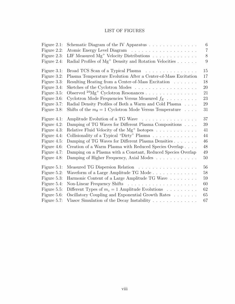
Figure 3.1: Broad TCS Scan of a Typical Plasma . . . . . . . . . . . . . . . 15Figure 3.2: Plasma Temperature Evolution After a Center-of-Mass Excitation 17Figure 3.3: Resulting Heating from a Center-of-Mass Excitation . . . . . . . 18Figure 3.4: Sketches of the Cyclotron Modes . . . . . . . . . . . . . . . . . . 20Figure 3.5: Observed 24Mg+ Cyclotron Resonances . . . . . . . . . . . . . . . 21Figure 3.6: Cyclotron Mode Frequencies Versus Measured fE . . . . . . . . . 23Figure 3.7: Radial Density Profiles of Both a Warm and Cold Plasma . . . . 29Figure 3.8: Shifts of the mθ = 1 Cyclotron Mode Versus Temperature . . . . 31

Figure 4.1: Amplitude Evolution of a TG Wave . . . . . . . . . . . . . . . . 37Figure 4.2: Damping of TG Waves for Different Plasma Compositions . . . . 39Figure 4.3: Relative Fluid Velocity of the Mg+ Isotopes . . . . . . . . . . . . 41Figure 4.4: Collisionality of a Typical “Dirty” Plasma . . . . . . . . . . . . . 44Figure 4.5: Damping of TG Waves for Different Plasma Densities . . . . . . . 46Figure 4.6: Creation of a Warm Plasma with Reduced Species Overlap . . . . 48Figure 4.7: Damping on a Plasma with a Constant, Reduced Species Overlap 49Figure 4.8: Damping of Higher Frequency, Axial Modes . . . . . . . . . . . . 50

Figure 5.1: Measured TG Dispersion Relation . . . . . . . . . . . . . . . . . 56Figure 5.2: Waveform of a Large Amplitude TG Mode . . . . . . . . . . . . . 58Figure 5.3: Harmonic Content of a Large Amplitude TG Wave . . . . . . . . 59Figure 5.4: Non-Linear Frequency Shifts . . . . . . . . . . . . . . . . . . . . 60Figure 5.5: Different Types of mz = 1 Amplitude Evolutions . . . . . . . . . 62Figure 5.6: Oscillatory Coupling and Exponential Growth Rates . . . . . . . 65Figure 5.7: Vlasov Simulation of the Decay Instability . . . . . . . . . . . . . 67

viii

LIST OF TABLES

Table 4.1: Plasma Compositions . . . . . . . . . . . . . . . . . . . . . . . . . 36

ix

ACKNOWLEDGEMENTS

First and foremost, I would like to thank Dr. Fred Driscoll and Dr. Francois

Anderegg. I started graduate school with very little experimental expertise, and

it was only through their guidance that I became the experimentalist I am today.

Dr. Driscoll, my advisor, constantly challenged me to focus on the fundamentals

of the problem. He taught me the type of critical thinking that is required to be a

good experimentalist. The sum of my knowledge of optics, vacuum technology, and

electronic repair I owe to the patient and lucid explanations of Dr. Anderegg. He was

always willing to explain the basics, and taught me good experimental practices.

I also owe a debt of gratitude to the group theorists Dr. Tom O’Neil and Dr.

Dan Dubin. My decision to studying plasma physics was heavily influenced by my

first year electrodynamics course taught by Dr. O’Neil, and I am grateful that I made

that decision. Most of the theory in this dissertation comes from Dr. Dubin. He was

always available to answer questions, and help interpret the experimental results.

Lastly, I would like to thank my family and friends. My parents who have

always been supportive of my endeavors. I would not have made it this far without

your encouragement. My brother Ben for getting me to take time off to hangout; it

is always fun to beat you at fishing. And Cody Chapman, my roommate and fellow

graduate student, for taking my mind off work with ridiculous TV and hours of playing

Skyrim (“what a waste”).

This research was supported financially by the National Science Foundation

Grant PHY-1414570, and the Department of Energy Grants DE-SC0002451 and

DE-SC0008693.

Chapters 2 and 3, in part, are a reprint of the material as it appears in

x

three journal articles: M. Affolter, F. Anderegg, D. H. E. Dubin, and C. F. Driscoll,

Physics Letters A, 378, 2406 (2014); M. Affolter, F. Anderegg, D.H.E. Dubin and

C.F. Driscoll, Physics of Plasmas, 22, 055701 (2015); and M. Affolter, F. Anderegg,

C.F. Driscoll, Journal of the American Society for Mass Spectrometry, 26, 330 (2015).

The dissertation author was the primary investigator and author of these papers.

Chapter 4, in part, is currently being prepared for submission for publication.

M. Affolter, F. Anderegg, D.H.E. Dubin and C.F. Driscoll. The dissertation author

was the primary investigator and author of this material.

Chapter 5, in part, is currently being prepared for submission for publication. M.

Affolter, F. Anderegg, D.H.E. Dubin, F. Valentini and C.F. Driscoll. The dissertation

author was the primary investigator and author of this material.

xi

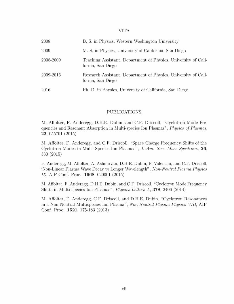
VITA

2008 B. S. in Physics, Western Washington University

2009 M. S. in Physics, University of California, San Diego

2008-2009 Teaching Assistant, Department of Physics, University of Cali-fornia, San Diego

2009-2016 Research Assistant, Department of Physics, University of Cali-fornia, San Diego

2016 Ph. D. in Physics, University of California, San Diego

PUBLICATIONS

M. Affolter, F. Anderegg, D.H.E. Dubin, and C.F. Driscoll, “Cyclotron Mode Fre-quencies and Resonant Absorption in Multi-species Ion Plasmas”, Physics of Plasmas,22, 055701 (2015)

M. Affolter, F. Anderegg, and C.F. Driscoll, “Space Charge Frequency Shifts of theCyclotron Modes in Multi-Species Ion Plasmas”, J. Am. Soc. Mass Spectrom., 26,330 (2015)

F. Anderegg, M. Affolter, A. Ashourvan, D.H.E. Dubin, F. Valentini, and C.F. Driscoll,“Non-Linear Plasma Wave Decay to Longer Wavelength”, Non-Neutral Plasma PhysicsIX, AIP Conf. Proc., 1668, 020001 (2015)

M. Affolter, F. Anderegg, D.H.E. Dubin, and C.F. Driscoll, “Cyclotron Mode FrequencyShifts in Multi-species Ion Plasmas”, Physics Letters A, 378, 2406 (2014)

M. Affolter, F. Anderegg, C.F. Driscoll, and D.H.E. Dubin, “Cyclotron Resonancesin a Non-Neutral Multispecies Ion Plasma”, Non-Neutral Plasma Physics VIII, AIPConf. Proc., 1521, 175-183 (2013)

xii

ABSTRACT OF THE DISSERTATION

Experimental Studies of Multi-Species Pure Ion Plasmas: CyclotronModes, Long-Range Collisional Drag, and Non-Linear Langmuir Waves

by

Matthew Affolter

Doctor of Philosophy in Physics

University of California, San Diego, 2016

Professor C. Fred Driscoll, Chair

Cyclotron modes are studied on rigid rotor, multi-species ion plasmas confined in

a Penning-Malmberg trap. Collective effects and radial electric fields shift the cyclotron

mode frequencies away from the “bare” cyclotron frequencies 2πF(s)c ≡ (qsB/Msc) for

each species s. These frequency shifts are measured on the distinct cyclotron modes

(mθ = 0, 1, and 2) with cos(mθθ) azimuthal dependence. We find that the frequency

shifts corroborate a simple theory expression in which collective effects enter only

through the E×B rotation frequency fE and the species fraction δs, when the plasma

is radially uniform. At ultra-low temperatures, these plasmas exhibit centrifugal

xiii

separation by mass, and additional frequency shifts are observed in agreement with a

more general theory. Additionally, quantitative measurements of the plasma heating

from short resonant cyclotron bursts are found to be proportional to the species

fraction.

These cyclotron modes are used as a diagnostic tool to estimate the plasma

composition, in order to investigate the damping of Langmuir waves due to inter-species

collisions. Experiments and theory of this collisional inter-species drag damping are

presented. This also provides the first experimental confirmation of recent theory

predicting enhanced collisional slowing due to long-range collisions. Drag damping

theory, proportional to the collisional slowing rate, is in quantitative agreement with

the experimental results only when these long-range collisions are included, exceeding

classical collision calculations by as much as an order of magnitude.

At large wave amplitudes, Langmuir waves exhibit harmonic generation, non-

linear frequency shifts, and a parametric decay instability, which are experimentally

investigated. The parametric wave-wave coupling rates are in agreement with three-

wave instability theory in the dispersion dominated oscillatory coupling regime, and

in the phase-locked exponential decay regime. However, significant variations are

observed near the decay threshold, including slow, oscillatory growth of the daughter

wave amplitude. These experimental results have motivated wide-ranging theory and

simulations, which provide both insights and puzzles.

xiv

Chapter 1

Introduction and Overview

Plasmas consisting of a single sign of charge, commonly referred to as non-

neutral plasmas, possess the important property that they can be confined in a state

of global thermal equilibrium by a combination of static electric and magnetic fields,

called a Penning-Malmberg trap [1]. The thermal equilibrium state is characterized

by the plasma temperature T , density n0, and radius Rp. These plasmas are well

controlled and diagnosed, enabling precise measurements of many physical processes

over a wide range of densities and temperatures.

Non-neutral ion plasmas are used to study a broad range of physics including

quantum simulations [2], spectroscopy [3], and basic plasma physics [4]. Rarely do

these pure ion plasmas consist of a single-species. Plasma sources routinely contain

multiple species and isotopes [5, 6], and unwanted impurity ions often arise from

ionization and chemical reactions with the neutral background gas [7, 8, 9]. These

impurities are difficult to diagnose, and they introduce complex multi-species plasma

phenomena. The majority of this dissertation is concerned with methods of diagnosing

these impurities, and on the multi-species effects they introduce.

1

2

Chapter 2 presents the details of the IV apparatus [5] on which these ex-

periments are conducted. This is a laser-diagnosed Penning-Malmberg trap with a

Magnesium plasma source. A brief overview of the trap geometry and “rotating-wall”

technique will be discussed, along with details of the laser diagnostics and cooling of

these ion plasmas.

Methods of diagnosing the species fractions through cyclotron modes are

presented in Chapter 3. We will describe a new laser-thermal cyclotron spectroscopy

technique, which detects mode resonances at very low amplitudes. This technique

enables detailed observations of surface cyclotron modes with mθ = 0, 1, and 2. For

each species s, we observe cyclotron mode frequency shifts that depend on the plasma

density through the rotation frequency, and on the charge concentration of species s, in

close agreement with recent theory. This includes the novel mθ = 0, radial “breathing”

mode, which generates no external electric field except at the plasma ends. These

cyclotron frequency shifts can be used to determine the plasma rotation frequency and

the species charge concentrations, in close agreement with our laser diagnostics. These

new results give a physical basis for the “space charge” and “amplitude” calibration

equations of cyclotron mass spectroscopy [10], widely used in molecular chemistry and

biology.

In Chapter 4, damping measurements of small amplitude Langmuir waves are

presented, spanning a range of four decades in temperature. These Langmuir waves

are θ-symmetric, standing plasma oscillations discretized by the axial wavenumber

kz = mzπ/Lp. At high temperatures (T ∼ 0.5 eV), these axial plasma waves are

Landau damped [11], but this prototypical Landau damping becomes exponentially

weak for T . 0.2 eV. However, we believe that Landau damping is extended to a lower

3

temperature regime (0.02 . T . 0.2 eV) through the same Landau interaction acting

on “bounce-harmonics” of the wave, caused by finite-length effects. The primary

interest of this chapter will be on the low temperature regime (T . 10−2 eV) where

the damping scales roughly as T−3/2 and is dependent on the plasma composition,

suggesting inter-species drag as the damping mechanism.

This inter-species drag damping provides a test of recent collision theory [12],

which predicts that the parallel slowing rate of these magnetized plasmas is enhanced

through long-range collisions. Drag damping theory, proportional to the parallel

slowing rate, is presented. We find that this drag damping theory is in quantitative

agreement with the experimental results only when long-range collisions are included,

exceeding classical collision calculations by as much as an order of magnitude.

The non-linear effects of frequency shifts, harmonic content, and instability of

large amplitude Langmuir waves are presented in Chapter 5. We characterize non-linear

frequency shifts and Fourier harmonic content versus amplitude, both of which are

increased when the wave dispersion is made more nearly acoustic. Non-linear coupling

rates are measured between large amplitude mz = 2 waves and small amplitude

mz = 1 waves, which have a small frequency detuning ∆ω ≡ 2ω1 − ω2. At small

excitation amplitudes, this detuning causes the mz = 1 mode amplitude to “bounce”

at rate ωB ≈ ∆ω, with amplitude excursions A1 ∝ δn2/n0 in quantitative agreement

with cold fluid theory [13] and Vlasov simulations. At larger excitation amplitudes,

where the non-linear coupling rate exceeds the detuning, phase-locked exponential

growth of the mz = 1 mode is observed, consistent with the three-wave instability

theory [13]. Significant variations are observed experimentally near the decay threshold,

including an average growth of the daughter wave amplitude before the phase-locked

4

regime. A recent cold fluid analysis [14] that considers frequency harmonics of these

large amplitude waves give stunningly divergent instability predictions that depend

sensitively on the dispersion-moderated harmonic content.

Chapter 2

Experimental Apparatus

2.1 IV Apparatus

These experiments are conducted on pure ion plasmas confined in a Penning-

Malmberg trap, as shown in Fig. 2.1. A Magnesium vacuum electrode arc [15] creates

a neutralized plasma, and the free electrons stream out through the +180 V end

confinement potentials, leaving Ntot ∼ 2 × 108 ions in a cylindrical column with

a length Lp ∼ 10 cm. Radial confinement is provided by the axial magnetic field

B = 2.965 ± 0.002 Tesla (−z). The ions are predominately Mg+ in three isotopic

states, with natural abundances 79% 24Mg+, 10% 25Mg+, and 11% 26Mg+. Other

impurity ions, mostly of H3O+, arise from chemical reactions with the background

gas. By changing the background gas pressure over the range 10−10 ≤ P ≤ 10−8 Torr,

the impurity ion fraction is varied from 5− 30%.

A “rotating wall” (RW) technique [16] utilizes azimuthally rotating wall voltages

to maintain the plasma in a near rigid-rotor equilibrium state for days. By altering

the frequency of this RW, the plasma can be arranged to a desired density n0, rotation

5

6

Rotating!Wall!

Cooling'Beam'Probe'Beam'

y'

x'z'

Figure 2.1: Schematic diagram of the IV apparatus. A cylindrical Penning-Malmberg trap with “rotating wall” and laser diagnostics.

frequency fE ≡ vθ/r, and radius Rp. The ion densities range over n0 = (0.9 →

6.4)× 107 cm−3, with rotation rates fE = (4→ 31) kHz, and inversely varying radii

Rp = (6→ 3) mm. The plasma length Lp and wall radius Rw = 2.86 cm remain fixed.

2.2 Laser Diagnostics

Detailed measurements of these Mg+ plasmas are obtained from laser induced

fluorescence techniques [5]. Figure 2.2 diagrams the Mg+ atomic energy levels, and

the two cyclic transitions that are in the near UV (λ ∼ 280 nm). In these experiments,

we use the 3S1/2,mj =−1/2 → 3P3/2,mj =−3/2 transition (blue dashed arrow) at

a frequency f0 ∼ 1.1 × 1015 Hz for laser diagnostics. A tunable, CW dye laser is

frequency-doubled to create a UV probe beam, which can be sent through the plasma

either perpendicular or parallel to the magnetic field. The frequency fL of this probe

beam is scanned over the Doppler-broadened atomic transition of each Mg+ isotope.

The excited ion state decays immediately and the resulting fluorescence photons are

7

3P3/2%

3S1/2%

+%3/2%+%1/2%)%1/2%)%3/2%

+%1/2%)%1/2%

279.55%nm%

+ΔE

ΔE−

mj%

Figure 2.2: Energy level diagram of a Mg+ ion. The Zeeman effect splits the3S1/2 and 3P3/2 levels (dotted) into magnetic field dependent energy states.The arrows illustrate the cyclic transitions used for laser diagnostics andcooling (blue dashed), and for magnetic field calibration (red/blue).

counted using a photomultiplier tube. From this detected photon count rate, we

construct the Mg+ velocity distribution.

Figure 2.3 shows raw data and 3-isotope Voigt fits to the typical Mg+ distribu-

tions resulting from a perpendicular probe laser scan at three radial (x) locations in

the plasma. For r > 0, the velocity distributions are positively and negatively detuned

from the vθ = 0 resonance due to a Doppler shift from the plasma rotation, either

away from or towards the probe laser beam in the (−y) direction. This detuning is a

direct measurement of the E ×B rotation profile vθ(r). Radial profiles of the plasma

temperature T (r) and Mg+ density nMg(r) can also be obtained by fitting the velocity

distribution at each radial location with Voigt distributions for each Mg+ isotope.

Shown in Fig. 2.4 are the measured density and rotation profiles (symbols) at

three different rotation rates. These profiles are a convolution of the true “top-hat”

plasma profile with the finite size (∆x half-width σL ∼ 0.39 mm) probe laser beam. We

obtain the true plasma radius Rp and rotation frequency fE by fitting to a convolved

8

0

2

4

6

8

-4 -2 0 2 4 6

-100 -50 0 50 100 150

Det

ecte

d Ph

oton

Rat

e

Laser Frequency Detuning [GHz]

[106 /

(sec

mW

)]

x = -0.1 mm

x = -3.1 mmx = 3.2 mm

vθ [103 cm / sec]

T ~ 10-2 eV

Figure 2.3: Data and fits of the LIF measured Mg+ velocity distributionsat three radial locations r ≡ |x| in the plasma. At each location, the largerpeak is the distribution of 24Mg+, and the smaller hump is the combineddistributions of 25Mg+ and 26Mg+.

“top-hat” model with constant n(r) = nMg and vθ(r) = 2πrfE for r ≤ Rp, giving the

dashed curves in Fig. 2.4. The solid lines in Fig. 2.4 are the resulting true “top-hat”

Mg+ density and rigid-rotor rotation profiles of the plasma. This rigid-rotor rotation

frequency fE is a direct measurement of the total electric field strength from ion space

charge and trap potentials.

2.3 RZ Poisson-Boltzmann Solver

A RZ Poisson-Boltzmann solver extends these measured radial cross-sections

to determine the plasma length. This solver iterates the RZ density n(r, z) to establish

9

0

1

2

3

4M

g+ Den

sity

[107 c

m-3

]Rp = 3.51 mm

Rp = 4.18 mm

Rp = 5.65 mm

2σL

0

10

20

30

40

50

60

0 1 2 3 4 5 6 7

V θ [1

03 cm

/sec

]

r [mm]

Shot #2363

fE = 24.5 kHz fE = 17.1kHz

fE = 9.3 kHz

Figure 2.4: Radial profiles of Mg+ density (Top) and rotation velocities(Bottom) at three different rotation rates for a T ∼ 10−2 eV plasma. Symbolsare laser-width-averaged data, and dashed curves are fits to the “top-hat”rigid-rotor model (solid lines). The three circled/boxed data points correspondto the LIF signals of Fig. 2.3.

10

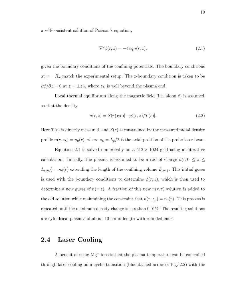
a self-consistent solution of Poisson’s equation,

∇2φ(r, z) = −4πqn(r, z), (2.1)

given the boundary conditions of the confining potentials. The boundary conditions

at r = Rw match the experimental setup. The z-boundary condition is taken to be

∂φ/∂z = 0 at z = ±zE, where zE is well beyond the plasma end.

Local thermal equilibrium along the magnetic field (i.e. along z) is assumed,

so that the density

n(r, z) = S(r) exp[−qφ(r, z)/T (r)]. (2.2)

Here T (r) is directly measured, and S(r) is constrained by the measured radial density

profile n(r, zL) = n0(r), where zL = Lp/2 is the axial position of the probe laser beam.

Equation 2.1 is solved numerically on a 512 × 1024 grid using an iterative

calculation. Initially, the plasma is assumed to be a rod of charge n(r, 0 ≤ z ≤

Lconf ) = n0(r) extending the length of the confining volume Lconf . This initial guess

is used with the boundary conditions to determine φ(r, z), which is then used to

determine a new guess of n(r, z). A fraction of this new n(r, z) solution is added to

the old solution while maintaining the constraint that n(r, zL) = n0(r). This process is

repeated until the maximum density change is less than 0.01%. The resulting solutions

are cylindrical plasmas of about 10 cm in length with rounded ends.

2.4 Laser Cooling

A benefit of using Mg+ ions is that the plasma temperature can be controlled

through laser cooling on a cyclic transition (blue dashed arrow of Fig. 2.2) with the

11

rest-frame resonance ω0. An ion moving with velocity v is then resonant at a laser

frequency ω(~v) = ω0 + ~k · ~v, where ~k = ω0/c is the laser wavenumber. By tuning the

axial cooling laser (±z) to a frequency slightly below ω0, ions moving with a specific

velocity vc towards the laser will be resonantly excited, and receive a momentum “kick”

decreasing the ion velocity. These excited ions will then remit a photon in a random

direction. On average, this absorbtion/emission cycle results in a reduction in the

ions velocity, and thus cooling of the plasma along the parallel (z) degree of freedom.

Perp-to-parallel collisions at a rate ν⊥‖ then cool the perpendicular degree of freedom.

In these experiments, the plasma temperature is controlled over the range

(10−5 → 1) eV through laser cooling of the 24Mg+ ions. This corresponds to a several

decade change in the perp-to-parallel collisionality ν⊥‖ = (104 → 1) s−1, and in the

Debye length λD = (0.005→ 1.7) mm. The radial distribution of ion species is also

temperature dependent through the effect of centrifugal mass separation [17, 18, 19, 20].

For plasmas at T & 10−2 eV, the ions species are uniformly mixed. In contrast, at

T < 10−3 eV, the species begin to centrifugally separate by mass, with near-complete

separation at T < 10−4 eV. This is discussed in Section 3.6.

2.5 Magnetic Field Calibration

Chapter 3 of this dissertation deals with cyclotron mode frequency shifts

on the order of a percent of the “bare” cyclotron frequency. To understand these

frequency shifts, we calibrated the magnetic field strength in the confinement volume

by measuring the Zeeman splitting of the Mg+ atomic levels. As shown in Fig. 2.2,

the atomic energy levels are split, and this spacing is dependent on the magnetic

field strength. The energy (or frequency) difference between the two cyclic transition,

12

illustrated by the arrows in Fig. 2.2, is

∆EZ ≡ ∆E+ −∆E− = h∆fZ = 28.0136hB [GHz/Tesla]. (2.3)

A 120 GHz scan in the UV covering these two cyclic transitions finds ∆fZ = 83.06±0.06

GHz, corresponding to a magnetic field strength of B = 2.965 ± 0.002 Tesla. This

10−3 accuracy is maintained for all experiments.

2.6 Acknowledgements

This chapter, in part, is a reprint of the material as it appears in three journal

articles: M. Affolter, F. Anderegg, D. H. E. Dubin, and C. F. Driscoll, Physics Letters

A, 378, 2406 (2014); M. Affolter, F. Anderegg, D.H.E. Dubin and C.F. Driscoll, Physics

of Plasmas, 22, 055701 (2015); and M. Affolter, F. Anderegg, C.F. Driscoll, Journal of

the American Society for Mass Spectrometry, 26, 330 (2015). The dissertation author

was the primary investigator and author of these papers.

Chapter 3

Cyclotron Mode Frequencies and

Resonant Absorption

3.1 Introduction

Plasmas exhibit a variety of cyclotron modes, which are used in a broad range

of devices to manipulate and diagnose charged particles. In fusion devices, cyclotron

modes are used for plasma heating [21, 22, 23], and the intensity of the plasma

cyclotron emission provides a diagnostic of the plasma temperature [24, 25]. Cyclotron

modes in ion clouds are widely used in molecular chemistry and biology to precisely

measure ion mass. In these plasmas, with a single sign of charge [26, 27, 28], collective

effects and electric fields shift the cyclotron mode frequencies away from the “bare”

cyclotron frequencies 2πF(s)c ≡ (qsB/Msc) for each species s. Mass spectroscopy

devices typically attempt to mitigate these effects with the use of calibration equations,

but these equation commonly neglect collective effects [29] or conflate them with

amplitude effects [27].

13

14

Here we quantify the shifts of cyclotron mode frequencies for several cyclotron

modes varying as cos(mθθ − 2πf(s)mθt). The mθ = 1 mode represents an orbit of the

center-of-mass, and is the most commonly utilized mode. We also quantify the plasma

heating from resonant wave absorption of the mθ = 1 mode. These measurements are

conducted on well-controlled, laser-diagnosed, multi-species ion plasmas, with near

uniform charge density n0 characterized by the near-uniform E×B rotation frequency

fE ≡ cen0/B. On these radially uniform plasmas, the cyclotron mode frequency shifts

are proportional to fE, with a constant of proportionality dependent on the species

fraction δs ≡ ns/n0, as predicted by the simple theory expression [7, 30, 31] of Eq. 3.4.

The plasma heating from resonant wave absorption is analyzed quantitatively using a

center-of-mass model. We find that the plasma heating and cyclotron mode frequency

shifts can be used as diagnostic tools to measure the species fractions δs.

The cyclotron mode frequencies are also investigated on plasmas with non-

uniform species distributions ns(r). The radial distribution of species is controlled

through the effects of centrifugal mass separation [17, 18, 19, 20]. When the species

are well separated radially, each cyclotron mode frequency depends on the “local”

concentration of that species. These measurements are in agreement with a more

general theory [30, 31] involving a radial integral over ns(r), with a simple asymptote

for complete separation into distinct annuli.

3.2 Thermal Cyclotron Spectroscopy

Thermal Cyclotron Spectroscopy (TCS) is used to detect the cyclotron reso-

nances. A cartoon of this process is shown in the inset of Fig. 3.1. A series of RF

bursts, scanned over frequency, are applied to an azimuthally sectored confinement ring.

15

0

1000

2000

3000

4000

5000

6000

20 25 30 35 40

ion mass [amu]

Fluo

resc

ence

[co

unts

/10m

s]

Burst Frequency [kHz]2800 2300 1800 1300

O2

+H3O+

24Mg+

25Mg+

26Mg+

mθ = 1 modesFile #38584

0

0.5

1

-150 -100 -50 0 50 100 150

F( v // )

v// [103 cm / sec]

initial 24Mg+

distribution

heated 24Mg+

distribution

coolingfluorescence

increases

cooling laserfrequency

Figure 3.1: Broad TCS scan of a typical plasma containing 24Mg+, 25Mg+,and 26Mg+; with H3O

+ and O+2 impurity ions. This mass spectra is obtained

by monitoring the plasma heating from resonant wave absorption throughthe cooling laser fluorescence, as depicted in the inset cartoon.

Resonant wave absorption heats the plasma, changing the 24Mg+ velocity distribution,

which is detected through LIF diagnostics.

Figure 3.1 shows a broad TCS scan used to identify the composition of a “dirty”

plasma. Here the plasma heating is detected as an increase in the cooling fluorescence,

and we use a long RF burst of 104 cycles to obtain a narrow frequency resolution. As

expected, the plasma consist of 24Mg+, and the Magnesium isotopes 25Mg+ and 26Mg+.

Ions of mass 19 amu and 32 amu are also typically observed, which we believe to be

H3O+ and O+

2 , resulting from ionization and chemical reactions with the background

gas at a pressure of P ∼ 10−9 Torr. Typical “dirty” plasma isotopic charge fractions

are δ24 = 0.54, δ25 = 0.09, δ26 = 0.10, with the remaining 27% a mixture of H3O+ and

16

O+2 .

3.3 Resonant Heating

To quantify the resultant heating from resonant wave absorption, we measure

the time evolution of the parallel velocity distribution F (v‖, t) concurrent with a

resonant RF burst. This entails detuning the probe laser frequency to a v‖ in the

Mg+ distribution. The cooling beam is then blocked, a cyclotron mode is excited, and

the arrival time of each detected photon is recorded. By repeating this process for

100 different probe detuning frequencies (i.e. parallel velocities), F (v‖, t) is measured

for specified time bins. These distributions are fit by Maxwellian distributions to

construct the time evolution of the plasma temperature.

Figure 3.2 shows the resulting temperature evolution for the excitation of the

center-of-mass mode of 24Mg+ at three different burst amplitudes AB. In this case,

the plasma is initially cooled to T ∼ 10−3 eV, and the heating due to collisions with

the room temperature background gas is negligible, at about 1.7× 10−6 eV/ms. At

20 ms, the cyclotron mode is excited using a 200 cycle burst at f(24)1 = 1894.6 kHz,

corresponding to a burst period τB = 0.1 ms. The plasma temperature increases by

∆Ts on a 10 ms time scale as the cyclotron energy is deposited isotropically as heat in

the plasma, through ion-ion collisions.

We find ∆Ts ∝ (δs/Ms)(ABτB)2 for short bursts τB . 0.1 ms, as shown in

Fig. 3.3. Here the center-of-mass mode of 24Mg+ and 26Mg+ are excited at f(24)1 =

1894.6 kHz and f(26)1 = 1745.2 kHz, with short bursts of 100 and 200 cycles. The

amount of heating is dependent on the concentration of the species δs, with the

majority species 24Mg+ heating the plasma about 4× more than the minority species

17

0

5

10

15

20

0 20 40 60 80 100 120 140

T [1

0-3 e

V ]

time [ms]

Shot #2448

No Burst

AB = 5.5 Vpp

AB = 7.5 Vpp

AB = 9.5 Vpp

ΔT24 = 10-2 eV

Burs

t

≈

Figure 3.2: Time evolution of the plasma temperature after the excitationof the center-of-mass mode of 24Mg+ at three different burst amplitudes AB.A 200 cycle RF burst at f

(24)1 = 1894.6 kHz is used, corresponding to a short

burst period τB = 0.1 ms.

26Mg+.

This ∆Ts scaling is consistent with a center-of-mass model. Consider an ion

initially at rest in the plasma, which is then excited at the species center-of-mass

cyclotron frequency ω(s)1 = 2πf

(s)1 by a sinusoidal electric field of amplitude E0. The

resulting motion can be model as an undamped driven harmonic oscillator,

r +[ω(s)1

]2r =

qsE0

Ms

sin[ω(s)1 t]. (3.1)

The amplitude of the driven cyclotron motion increases linearly in time, with an

average energy in an oscillation of

〈Es〉 ∝q2sMs

(ABτB)2, (3.2)

18

1

10

10-4 10-3

Δ Ts

[10-3

eV

]

AB τB [V s]

Shot #2448

24Mg+

26Mg+

mθ = 1 modes

δ 24δ 26

≈ 4

ΔT24 = 1.5 ×104 eVVs( )2 ABτ B( )2

ΔT26 = 3.4 ×103 eVVs( )2 ABτ B( )2

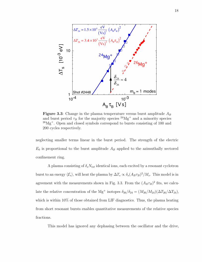
Figure 3.3: Change in the plasma temperature versus burst amplitude ABand burst period τB for the majority species 24Mg+ and a minority species26Mg+. Open and closed symbols correspond to bursts consisting of 100 and200 cycles respectively.

neglecting smaller terms linear in the burst period. The strength of the electric

E0 is proportional to the burst amplitude AB applied to the azimuthally sectored

confinement ring.

A plasma consisting of δsNtot identical ions, each excited by a resonant cyclotron

burst to an energy 〈Es〉, will heat the plasma by ∆Ts ∝ δs(ABτB)2/Ms. This model is in

agreement with the measurements shown in Fig. 3.3. From the (ABτB)2 fits, we calcu-

late the relative concentration of the Mg+ isotopes δ26/δ24 = (M26/M24)(∆T26/∆T24),

which is within 10% of those obtained from LIF diagnostics. Thus, the plasma heating

from short resonant bursts enables quantitative measurements of the relative species

fractions.

This model has ignored any dephasing between the oscillator and the drive,

19

which can result from collisions, damping, or an initially off-resonant burst. Dephasing

will result in less energy per ion, and a smaller ∆Ts. We find that the ∆Ts ∝ (ABτB)2

scaling is only valid for short bursts τB . 0.1 ms. As the burst period is increased,

keeping ABτB constant, we observe a decrease in the plasma heating. At a τB ∼ 1.7

ms (∼ 3000 cycles), the heating is decreased to less than 40% of the short burst

expectation, with a larger decrease for the minority species.

This dephasing for long bursts explains why the height of the peaks in Fig. 3.1

underestimate the concentrations of the minority species. At present it is unclear

what is causing the dephasing on this time scale. We have changed the initial plasma

temperature by an order of magnitude (10−3 → 10−2) eV to no effect, and the burst

frequency is accurate to a few hundred Hz, ruling out an off-resonant drive.

3.4 Radially Uniform Plasma

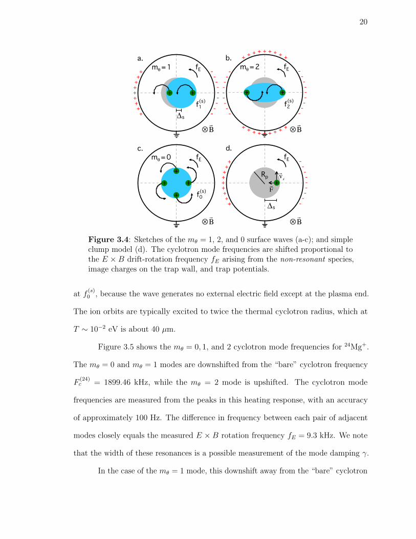
Frequency shifts are measured for the mθ = 0, 1, and 2 cyclotron modes having

density perturbations on the plasma radial surface varying as δn ∝ cos(mθθ− 2πf(s)mθt),

as shown in Fig. 3.4. For the mθ = 1 mode, the ion orbits are in phase, resulting in a

displacement of the center-of-mass of the exited species, which then orbits the center

of the trap at f(s)1 , as in Fig. 3.4 (a). This mode is excited by a dipole burst on an

azimuthally sectored confinement ring. A quadrupole burst can excite the “elliptical”,

mθ = 2 mode [32, 7]. As shown in Fig. 3.4 (b), this elliptical density perturbation,

rotating at f(s)2 , is created by a 180◦ phase shift of the ion orbits on opposite radial

edges of the plasma. The final mode we have analyzed is the novel mθ = 0, radial

“breathing” mode [33, 34, 35] in which the plasma cross-section expands and contracts

radially, as shown in Fig. 3.4 (c). To excite this mode, the end of the plasma is wiggled

20

mθ = 1!

f1!(s)!

Δs!

a.!+!

+!+!+!+!+!+!+!+! -!

-!-!-!-!-!-!-!-!fE!

mθ = 0! fE!

f0!(s)!

c.!

+!+!

+!+!+!+!+!+!+!

mθ = 2!

f2!(s)!

b.!

-!-!

-!-!-!-!-!-!-!fE!

+! +! +! +! +! +! +! +! +!

-!-!

-!-!-!-!-!-!-!

Δs!

d.!+!

+!+!+!+!+!+!+!+! -!

-!-!-!-!-!-!-!-!fE!

Rp! vs

F

⊗ B ⊗

B

⊗ B ⊗

B

Figure 3.4: Sketches of the mθ = 1, 2, and 0 surface waves (a-c); and simpleclump model (d). The cyclotron mode frequencies are shifted proportional tothe E ×B drift-rotation frequency fE arising from the non-resonant species,image charges on the trap wall, and trap potentials.

at f(s)0 , because the wave generates no external electric field except at the plasma end.

The ion orbits are typically excited to twice the thermal cyclotron radius, which at

T ∼ 10−2 eV is about 40 µm.

Figure 3.5 shows the mθ = 0, 1, and 2 cyclotron mode frequencies for 24Mg+.

The mθ = 0 and mθ = 1 modes are downshifted from the “bare” cyclotron frequency

F(24)c = 1899.46 kHz, while the mθ = 2 mode is upshifted. The cyclotron mode

frequencies are measured from the peaks in this heating response, with an accuracy

of approximately 100 Hz. The difference in frequency between each pair of adjacent

modes closely equals the measured E ×B rotation frequency fE = 9.3 kHz. We note

that the width of these resonances is a possible measurement of the mode damping γ.

In the case of the mθ = 1 mode, this downshift away from the “bare” cyclotron

21

2500

3000

3500

4000

4500

5000

1880 1885 1890 1895 1900 1905 1910

mθ = 1 mθ = 2

mθ = 0

Burst Frequency [kHz]

Fluo

resc

ence

[co

unts

/10m

s]

fE

File #49749

2γ

24Mg+

Fc(24)

fE

Figure 3.5: Observed 24Mg+ cyclotron resonances for mθ = 0, 1, and 2 modes.Modes are shifted away from the “bare” cyclotron frequency F

(24)c = 1899.46

kHz. These modes have a frequency spacing of approximately the E × Brotation frequency fE = 9.3 kHz.

frequency can be understood through a simple “clump” model. Sketched in Fig. 3.4

(d) is a cylindrical trap confining a multi-species ion plasma. A species is excited to

an amplitude ∆s, and undergoes uniform circular motion about the center of the trap

with a velocity vs, resulting in a frequency f(s)1 = vs/2π∆s. The dynamics of this

excited species can be modeled by a point particle located at the center-of-mass of

the excited species. The radial forces acting on this point particle are the centrifugal,

vs ×B, and electrostatic forces, summing to zero as

Msv2s

∆s

− qsc

vsBz + qsEr = 0. (3.3)

Here Er represents the electric field generated by the non-resonant species, trap

potentials, and image charge on the trap wall; rather than the total electric field

22

Er measured through fE. (That is, the clump cannot push on itself.) Equation 3.3

reduces to f(s)1 = F

(s)c when Er = 0. However, Er > 0 increases the outward radial

force, mandating a downshift in the center-of-mass mode frequency.

In these experiments, the radial electric field Er is controlled by compressing

the plasma with the RW, and the strength of this electric field is measured through the

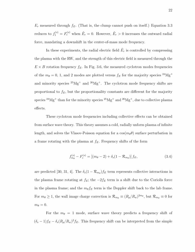
E ×B rotation frequency fE. In Fig. 3.6, the measured cyclotron modes frequencies

of the mθ = 0, 1, and 2 modes are plotted versus fE for the majority species 24Mg+

and minority species 25Mg+ and 26Mg+. The cyclotron mode frequency shifts are

proportional to fE, but the proportionality constants are different for the majority

species 24Mg+ than for the minority species 25Mg+ and 26Mg+, due to collective plasma

effects.

These cyclotron mode frequencies including collective effects can be obtained

from surface wave theory. This theory assumes a cold, radially unform plasma of infinite

length, and solves the Vlasov-Poisson equation for a cos(mθθ) surface perturbation in

a frame rotating with the plasma at fE. Frequency shifts of the form

f (s)mθ− F (s)

c = [(mθ − 2) + δs(1−Rmθ)] fE, (3.4)

are predicted [30, 31, 4]. The δs(1−Rmθ)fE term represents collective interactions in

the plasma frame rotating at fE; the −2fE term is a shift due to the Coriolis force

in the plasma frame; and the mθfE term is the Doppler shift back to the lab frame.

For mθ ≥ 1, the wall image charge correction is Rmθ ≡ (Rp/Rw)2mθ , but Rmθ ≡ 0 for

mθ = 0.

For the mθ = 1 mode, surface wave theory predicts a frequency shift of

(δs − 1)fE − δs(Rp/Rw)2fE. This frequency shift can be interpreted from the simple

23

1860

1880

1900

1920

Shot #2363

mθ = 0

mθ = 1

mθ = 224Mg+

Fc = 1899.22 kHz

δ24

= 53.4%

(24)

1780

1800

1820

1840

Cycl

otro

n M

ode

Freq

uenc

y f m

[

kHz]

mθ = 0

mθ = 1

mθ = 2

25Mg+

Fc = 1823.47 kHz

δ25

= 8.68%

(25)

(s)

Cycl

otro

n M

ode

Freq

uenc

y f m

[

kHz]

(s) θ

1700

1720

1740

1760

0 5 10 15 20 25 30fE [kHz]

mθ = 0

mθ = 1

mθ = 226Mg+

Fc = 1753.58 kHz

δ26

= 9.88%

(26)

Figure 3.6: Cyclotron mode frequencies versus measured fE for 24Mg+,25Mg+, and 26Mg+. Symbols are experimental data and curves are fits toEq. 3.4, which determine F

(s)c (dotted) and δs for each species.

24

clump model. The (δs − 1)fE term represents the radial electric field from the non-

resonant species. A species clump cannot exert a force on itself, reducing the effective

space charge electric field by δs. However, the image charges of the clump do exert a

force on the clump center-of-mass, represented here by a frequency shift of

f(s)D = δsfE

(Rp

Rw

)2

, (3.5)

equal to the species mθ = 1 diocotron frequency. In these experiments Rp << Rw, so

the dominant frequency shift is caused by the non-resonant species. The image charge

frequency shift f(s)D < 200 Hz, and is dependent on the concentration of the species.

Fitting Eq. 3.4 to the measured frequency shifts in Fig. 3.6, we find that the

observed mode frequency spacing is consistent to within the 2% accuracy of the LIF

measurements of fE, and that these cyclotron modes converge to the “bare” cyclotron

frequency F(s)c in the limit fE → 0. Also, the slope of the frequency shifts in Fig. 3.6

provide a measurement of the species fractions δs for each species. The relative Mg+

ratios δ25/δ24 and δ26/δ24 are within 20% of those obtained through LIF diagnostics,

and within 5% of that obtained from the resonant wave absorption technique. The

corresponding mass ratios from F(s)c are accurate to within 200 ppm.

Four frequencies f(s)mθ from two mθ modes in two plasma states could be used

to determine the plasma characteristics fE and δs, and thereby determine F(s)c . In

Fig. 3.6, the measured cyclotron frequency differences of the two circled (vertical) data

pairs give fE = (9.33, 16.97) kHz versus the measured (9.29, 17.13) kHz; and Eq. 3.4

then gives δ26 = 9.06% and F(26)c = 1753.82 kHz, in close agreement with the results

in Fig. 3.6. Of course, similar information from multiple species would improve this

plasma characterization.

25

This surface wave theory [30, 31, 4] has ignored finite-length effects resulting

from the trap end potentials. These effects have been measured on the low-frequency

diocotron mode in electron plasmas [36]. Extending these results to the plasma

conditions of our experiments, we find that finite-length effects produce a frequency

shift of approximately 50 Hz.

In a single species plasma (δ = 1), the frequency shifts from trap potentials

and image charge are dominant, because there are no non-resonant species. Prior

work [32] measured the center-of-mass cyclotron mode frequency on electron plasmas,

and found that the mθ = 1 mode is downshifted by the diocotron frequency fD due

to image charge in the conducting walls. Later multi-species work [7] described the

spacing between the mθ-modes in terms of several fD when image charges dominated.

This prior work was conducted on hot plasmas T ∼ 3 eV, with parabolic density

profiles extending to large Rp/Rw. In general, fE is the more fundamental parameter

describing these frequency shifts, since image charge forces are generally weak.

3.5 Mass Spectroscopy Calibration Equation

The accuracy of Fourier transform ion cyclotron resonance mass spectrometry

(FTICR-MS) is often limited by these cyclotron frequency shifts. Conversion from the

measured cyclotron frequency to a mass to charge ratio (M/q)s is typically done using

one of the several calibration equations [10], which correct for the space charge electric

field and its influence on the cyclotron frequency. In this section, we extend the simple

clump model to calculate a calibration equation consistent with our experimental

results.

26

Solving for (M/q)s in Eq. 3.3 produces a calibration equation,

(M

q

)s

=Bz

2πcf(s)1

− 1

(2πf(s)1 )2

Er∆s

. (3.6)

The accuracy of Eq. 3.6 depends on correctly modeling Er/∆s at the radial position

∆s of the clump. Note that Er/r represents the E × B drift rotation frequency as

fE(r) = (cEr/r)/2πB. In our experiments, fE is uniform with r.

When the equilibrium charge densities are uniform and the excitation amplitude

is small (i.e.,∆s < Rp), the electric field ratio Er/∆s is basically independent of radius.

Then, the “calibration” of Eq. 3.6 is independent of radius. The ion cloud is also

assumed to be long compared to its radius Lp >> Rp, so that the ion cloud and image

charge electric fields can be approximated as those of an infinitely long cylinder. The

partial electric field Er produced from the non-excited ion cloud species, from image

charges of the excited species, and from trap potentials VT is then

Er∆s

= 2π(1− δs)en0 + 2πδsen0R1 + 2VTGT , (3.7)

where en0 = Q0/πR2pLp is the total charge density, and GT is a trap-dependent

geometrical factor relating the z-averaged Er/r to the applied VT [37].

Here we see that the dependence on δs comes from the reduction of the effective

electric field, since the excited species clump cannot apply a force on itself; and from

the image charge in the confining wall, which does apply a force on the excited clump.

The image charges of the non-excited species are θ-symmetric, and the image charges

of any other excited species are assumed to be non-resonant and therefore time-average

to zero. By taking δs → 0 (i.e., treating a single particle excitation and ignoring image

27

charge), this electric field Er reduces to that of Jeffries et al. [37].

From this Er/∆s, a calibration equation can be obtained,

(M

q

)s

=

A︷︸︸︷Bz

2πc

1

f(s)1

+

[ B︷ ︸︸ ︷−(

2πen0 + 2VTGT

(2π)2

)+

C︷ ︸︸ ︷en0

{1−R1

2π

}δs

]1

(f(s)1 )2

. (3.8)

This calibration equation depends on the relative charge density δs of species s. If the

excitation amplitudes ∆s are the same for each species, then the received wall signal

Is is a measure of δs, and Eq. 3.8 results in the “intensity-dependent” calibration

equation of Refs [38, 27]. In general, Is is only an approximate measure of δs because

it is also proportional to the excitation amplitude as Is ∝ δs∆s. The parameters A and

B are identical to those of the simplest calibration equation in general use [29]. They

calibrate single particle effects such as the magnetic field strength, and frequency shifts

from the entire ion cloud and trap potentials. Parameter C corrects for overestimating

the frequency shift from the ion cloud when self forces between the excited species

and itself were included, and also includes the effects of image charge.

3.6 Non-Uniform Species Fractions

In this section, we investigate the cyclotron mode frequencies on plasmas with

radially non-uniform species fractions ns(r). The radial distribution of each species

varies because of centrifugal mass separation. When uniformly distributed, species of

different mass drift-rotate at slightly different rates, and therefore experience viscous

drags in the azimuthal direction. These drags produces Fdrag ×Bz radial drifts, which

radially separate each species and forms a more uniform rotation profile. The species

concentrate into separate radial annuli, each approaching the full plasma density n0,

28

with the lighter species on center.

The equilibrium density profiles of each species can be theoretically determined.

The ratio of densities between two species is equal to

na(r)

nb(r)= Cab exp

[1

2T(Ma −Mb)(2πfE)2r2

], (3.9)

where Cab is a constant determined by the overall fraction of each species [20]. The

effects of centrifugal mass separation are important for species with a large mass

difference and for cold plasmas.

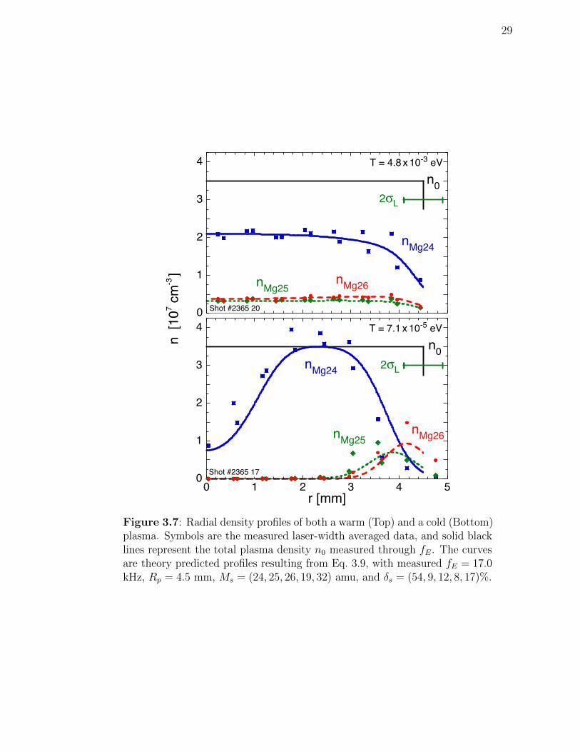
Shown in Fig. 3.7 are measured density profiles for both a warm plasma with

minimal separation, and a cold plasma with strong separation. The symbols represent

the LIF measured densities of the Mg+ isotopes, and the solid black line is the total

plasma density n0 measured through the E × B rotation frequency. The curves

are theory predicted profiles for the measured species fractions δs, plasma rotation

frequency fE, and “top-hat” radius Rp. These theory profiles have been convolved

with the finite size probe laser beam σL, so they can be compared directly with the

experimental measurements.

At T = 4.8× 10−3 eV, the species are uniformly mixed, as shown in Fig. 3.7

(Top). This is a typical example of a radially uniform plasma. Here the species

fractions δs ≡ ns/n0 are constant over the plasma radius, and the cyclotron mode

frequencies are well described by Eq. 3.4. Note that the sum of the Mg+ isotopes is

not equal to the total plasma density due to the presence of impurity ions, H3O+ and

O+2 , not detected by the LIF diagnostics.

As the plasma is cooled, the species centrifugally separate and concentrate

into radial annuli increasing the “local” ns(r). At T = 7.1× 10−5 eV, the 24Mg+ has

29

0

1

2

3

4

Shot #2365 20

n0

nMg24

nMg25nMg26

T = 4.8 x 10-3 eV

2σL

0

1

2

3

4

0 1 2 3 4 5r [mm]

Shot #2365 17

n0nMg24

nMg25nMg26

T = 7.1 x 10-5 eV

2σL

n [1

07 cm

-3 ]

Figure 3.7: Radial density profiles of both a warm (Top) and a cold (Bottom)plasma. Symbols are the measured laser-width averaged data, and solid blacklines represent the total plasma density n0 measured through fE. The curvesare theory predicted profiles resulting from Eq. 3.9, with measured fE = 17.0kHz, Rp = 4.5 mm, Ms = (24, 25, 26, 19, 32) amu, and δs = (54, 9, 12, 8, 17)%.

30

approached the full plasma density n0, pushing the heavier Mg+ isotopes to the radial

edge, as shown in Fig. 3.7 (Bottom). The central hole observed in the Mg+ density

profile is a result of the lighter impurity species H3O+. Although the radially-averaged

species fractions are unchanged, the peak “local” fractions δs(r) ≡ ns(r)/n0 have

increased for each species. We find that the cyclotron mode frequencies are dependent

on these peak “local” species fractions.

Shown in Fig. 3.8 are measurements of the mθ = 1 frequency shifts as the

“local” species concentrations are varied by altering the plasma temperature. These

shifts are measured on 24Mg+, 26Mg+, and H3O+. At T & 10−3 eV, the species are

uniformly mixed and the frequency shifts are approximately (δs − 1)fE, as predicted

by Eq. 3.4. Cooling the plasma increases the “local” species concentrations, and

decreases the mθ = 1 frequency shift. At the coldest temperatures T ∼ 10−4 eV, the

“local” 24Mg+ and H3O+ densities have approached the full plasma density n0, and

the center-of-mass cyclotron mode frequency is nearly the “bare” cyclotron frequency.

Similar frequency shifts are observed for both the mθ = 0 and mθ = 2 modes, offset

by (mθ − 1)fE.

The full cyclotron mode analysis was developed by Dubin in Ref. [31]. For

radially varying ion densities ns(r) or varying rotation fE(r), the mode resonances

at f(s)mθ are predicted by peaks in the real part of the admittance Re(Ymθ). Here

Ymθ ≡ I/V relates electrode displacement current I to electrode voltage V . It has a

frequency dependence of

Ymθ ∝ i(2πf)Gmθ + 1

Gmθ − 1, (3.10)

with

Gmθ ≡ −2mθ

R2mθw

∫ Rw

0

drβ(r) r2mθ−1

α(r) − β(r), (3.11)

31

-1

-0.8

-0.6

-0.4

-0.2

0

10-4 10-3 10-2

T (fE/17kHz)2 (Rp/4.8mm)2 [eV]

H3O+

( f1

- F

c )

/ f E

= ( δ

s - 1

)

Shot #2365-9

24Mg+

26Mg+

mθ = 1 modes

(s)

(s)

fE

~ 17 kHz

Radially'Uniform'Centrifugally'Separated'

≈

Figure 3.8: Normalized shifts of the mθ = 1 cyclotron mode frequencies for24Mg+, 26Mg+, and H3O

+, as the “local” species concentrations increase dueto centrifugal separation. Symbol shapes represent species; symbol fill distin-guishes measurements on three plasmas with slightly different compositions.The temperature T is scaled by the centrifugal energy of these plasmas, whichdiffer by approximately 25%. Curves are theory predictions assuming a typicalspecies concentration Ms = (24, 25, 26, 19, 32) amu with δs = (54, 9, 9, 8, 20)%.The four vertical lines are the FWHM of the 24Mg+ cyclotron resonance atvarious temperatures.

β(r) ≡ ns(r)

n0

fE(0), (3.12)

and

α(r) ≡ (f (s)mθ− F (s)

c + iγ/2π)− (mθ − 2)fE(r) +r

2

∂

∂rfE(r). (3.13)

Peaks in Re(Ymθ) occur when Gmθ → 1.

The curves in Fig. 3.8 are the shifts resulting from numerically integrating

Eq. 3.10 with ns(r) as predicted for centrifugal separation, Eq. 3.9. As the plasma is

cooled, the “local” ns(r) increases towards the full “top-hat” density n0: this isolates

the species, and removes frequency shifts from the electric field of other species. As a

32

result, the cyclotron mode frequencies are shifted towards the single-species δs = 1

limit with ordinate 0. Here, the remaining shifts due to image charge [31] and trap

electric fields are negligible. The discontinuity in the 24Mg+ theory curve is due to

multiple modes with different radial mode structure. Although multiple radial modes

have been observed on some plasmas they were not observed for this set of data

possibly due to stronger damping.

Varying the plasma temperature also changes the observed width of the cy-

clotron resonance as shown by the four vertical FWHM (2γ) bars in Fig. 3.8. At

high temperatures T & 10−2 eV, the observed resonance width is determined by the

frequency width of the drive, which is approximately 0.4 kHz. When the plasma is

cooled, the ion-ion collision frequency ν⊥‖ increases, and the observed resonance width

probably reflects collisional damping of the cyclotron modes, varying qualitatively like

ν⊥‖. For T . 10−3 eV, inter-species collisions are reduced by centrifugal separation

of the species, and the cyclotron resonance width is observed to remain constant at

approximately 6 kHz.

3.7 Bernstein Waves

At temperatures T & 0.1 eV, where ion-ion collisionality is small, we observed

multiple closely-spaced modes near Fc with spacing dependent on T . This mode

splitting is similar to that observed in electron plasmas [32]; but here this splitting

occurs for the mθ = 1 mode where no splitting was previously seen. Theory work in

progress analyzes radially standing Bernstein waves in multi-species ion plasmas [31],

and a connection to this theory is being pursued.

33

3.8 Conclusion

On radially uniform plasmas, the mθ = 0, 1, and 2 cyclotron mode frequencies

are shifted by radial electric fields and collective effects in agreement with surface

wave theory, Eq. 3.4. These frequency shifts can be used to measure the plasma E×B

rotation frequency fE, and species fractions δs. This quantitative understanding of

the frequency shifts give a physical basis for the “space charge” and “amplitude”

calibration equations commonly used in mass spectroscopy. For short bursts τB . 0.1

ms, the plasma heating from resonant wave absorption of the mθ = 1 mode is

found to be ∆Ts ∝ δs(ABτB)2/Ms, providing another diagnostic tool of δs. For non-

uniform plasmas, the cyclotron mode frequencies are dependent on the “local” species

concentrations, and the frequency shifts from non-resonant species are removed when

the excited species is completely separated.

3.9 Acknowledgements

This chapter, in part, is a reprint of the material as it appears in three journal

articles: M. Affolter, F. Anderegg, D. H. E. Dubin, and C. F. Driscoll, Physics Letters

A, 378, 2406 (2014); M. Affolter, F. Anderegg, D.H.E. Dubin and C.F. Driscoll, Physics

of Plasmas, 22, 055701 (2015); and M. Affolter, F. Anderegg, C.F. Driscoll, Journal of

the American Society for Mass Spectrometry, 26, 330 (2015). The dissertation author

was the primary investigator and author of these papers.

Chapter 4

Inter-species Drag Damping of

Langmuir Waves

4.1 Introduction

Collision rates are fundamental to our understanding of transport phenomena

in plasmas. In magnetized plasmas, the cyclotron radius rc is often less than the

Debye length λD, and classical 3D Boltzmann collisions are limited to short-range,

with impact parameters ρ < rc. Rarely considered in these magnetized plasmas are

long-range (rc < ρ < λD) collisions described by guiding centers interacting as they

move along the magnetic field. However, experiments and theory have shown that these

long-range collisions can enhance cross-field diffusion [39, 40], heat transport [41, 42],

and viscosity [43, 44] by orders of magnitude in regimes where λD > rc.

Recent theory [12] provides a precise analysis of these long-range collisions on

the parallel slowing rate in a magnetized plasma. A new fundamental length scale d

was identified, separating collisions into regimes: ρ < d where the colliding particles

34

35

can be treated as two-body, point-like Boltzmann collisions; and ρ > d a Fokker-Planck

regime where multiple weak collisions occur simultaneously. This theory predicts that

the rate of collisional slowing parallel to the magnetic field is strongly enhanced by

long-range collisions. This enhancement of the parallel slowing rate applies to Penning

trap plasmas for both matter and antimatter [45, 46, 47], for some astrophysical

plasmas [48], and even for the edge region of tokomak plasmas [49, 50, 51].

Here we present the first experimental confirmation of this enhanced collisional

slowing rate, obtained through measurements of the damping of Langmuir waves

in a multi-species ion plasma. Collisional drag damping theory predicts damping

proportional to the collisional slowing rate. The measured damping rates are in quan-

titative agreement with the theory when long-range collisions are included: exceeding

predictions considering only 3D Boltzmann, short-range collisions by as much as an

order of magnitude.

These measurements of collisional drag damping extend over a range of two

decades in temperature. When collisions are weak and the ion species are uniformly

mixed, the damping rates are proportional to the collisionality, scaling roughly as

T−3/2. The damping is reduced at low temperatures as centrifugal mass separation

(see Sec. 3.6) and collisional locking of the fluid elements becomes significant. At

ultra-low temperatures, the plasma approaches the moderately correlated regime, and

these damping measurements may provide insight into the collisionality of a correlated,

magnetized plasma.

36

4.2 Species Concentrations

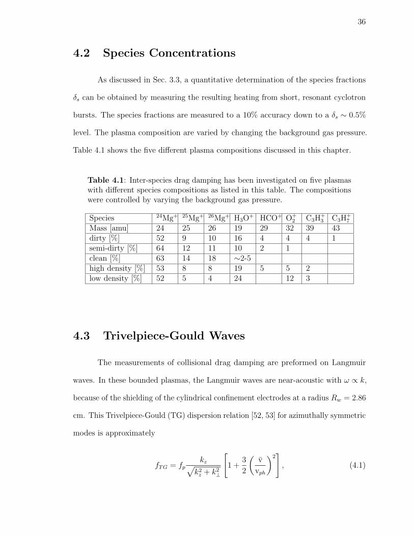
As discussed in Sec. 3.3, a quantitative determination of the species fractions

δs can be obtained by measuring the resulting heating from short, resonant cyclotron

bursts. The species fractions are measured to a 10% accuracy down to a δs ∼ 0.5%

level. The plasma composition are varied by changing the background gas pressure.

Table 4.1 shows the five different plasma compositions discussed in this chapter.

Table 4.1: Inter-species drag damping has been investigated on five plasmaswith different species compositions as listed in this table. The compositionswere controlled by varying the background gas pressure.

Species 24Mg+ 25Mg+ 26Mg+ H3O+ HCO+ O+

2 C3H+3 C3H

+7

Mass [amu] 24 25 26 19 29 32 39 43dirty [%] 52 9 10 16 4 4 4 1semi-dirty [%] 64 12 11 10 2 1clean [%] 63 14 18 ∼2-5high density [%] 53 8 8 19 5 5 2low density [%] 52 5 4 24 12 3

4.3 Trivelpiece-Gould Waves

The measurements of collisional drag damping are preformed on Langmuir

waves. In these bounded plasmas, the Langmuir waves are near-acoustic with ω ∝ k,

because of the shielding of the cylindrical confinement electrodes at a radius Rw = 2.86

cm. This Trivelpiece-Gould (TG) dispersion relation [52, 53] for azimuthally symmetric

modes is approximately

fTG = fpkz√

k2z + k2⊥

[1 +

3

2

(v

vph

)2], (4.1)

37

10-4

10-3

10-2

0 5 10 15 20 25 30 35 40

1

10

δn / n

0

Time [ms]

γ = 132 s-1T = 2.7 x 10-3 eVf1 = 26.05 kHz

vf [m /

s]

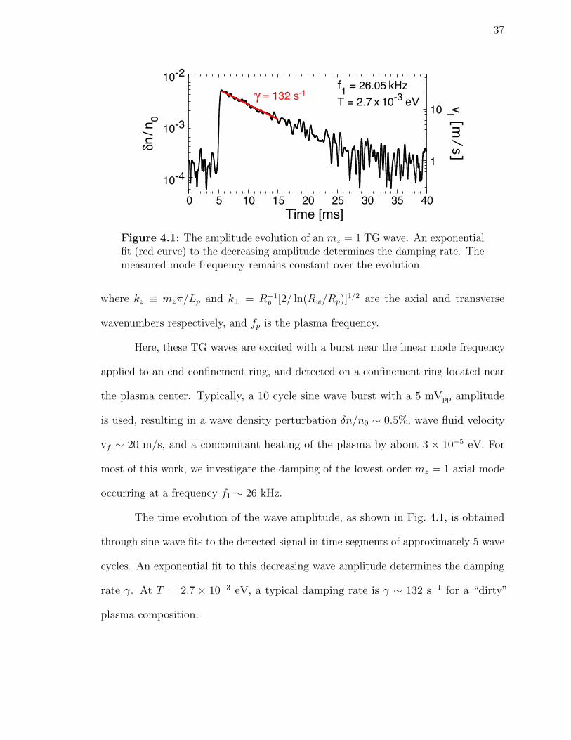
Figure 4.1: The amplitude evolution of an mz = 1 TG wave. An exponentialfit (red curve) to the decreasing amplitude determines the damping rate. Themeasured mode frequency remains constant over the evolution.

where kz ≡ mzπ/Lp and k⊥ = R−1p [2/ ln(Rw/Rp)]1/2 are the axial and transverse

wavenumbers respectively, and fp is the plasma frequency.

Here, these TG waves are excited with a burst near the linear mode frequency

applied to an end confinement ring, and detected on a confinement ring located near

the plasma center. Typically, a 10 cycle sine wave burst with a 5 mVpp amplitude

is used, resulting in a wave density perturbation δn/n0 ∼ 0.5%, wave fluid velocity

vf ∼ 20 m/s, and a concomitant heating of the plasma by about 3 × 10−5 eV. For

most of this work, we investigate the damping of the lowest order mz = 1 axial mode

occurring at a frequency f1 ∼ 26 kHz.

The time evolution of the wave amplitude, as shown in Fig. 4.1, is obtained

through sine wave fits to the detected signal in time segments of approximately 5 wave

cycles. An exponential fit to this decreasing wave amplitude determines the damping

rate γ. At T = 2.7 × 10−3 eV, a typical damping rate is γ ∼ 132 s−1 for a “dirty”

plasma composition.

38

4.4 Damping Measurements

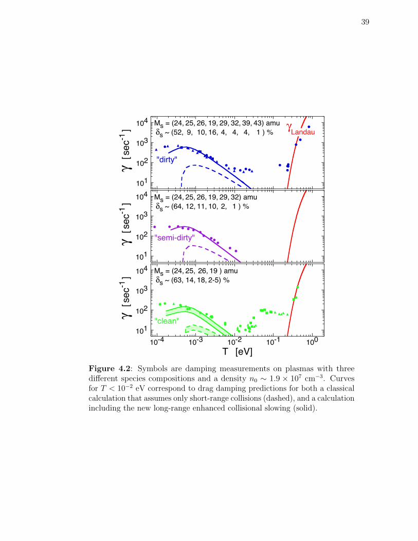
Figure 4.2 shows measurements of the damping rate over four decades in

the plasma temperature. At high temperatures (T ∼ 0.5 eV), collisionless Landau

damping dominates. Quantitative agreement with Landau theory is obtained for small

amplitude waves as indicated by the solid red curve [11]. This prototypical Landau

damping becomes exponentially weak for T . 0.2 eV. However, we believe the damping

in the regime 0.02 . T . 0.2 eV is a result of the same Landau interaction, but on

“bounce-harmonics” of the wave, caused by finite-length effects. Recent experiments [54]

conducted in this temperature regime have demonstrated that an externally applied

“squeeze” increases these wave harmonics, causing stronger damping in quantitative

agreement with recent bounce harmonic Landau damping theory [55].

At cryogenic temperatures (T . 10−2 eV), the damping is proportional to the

collisionality: dependent on the plasma composition and scaling roughly as T−3/2.

Figure 4.2 shows damping measurements on plasmas with three different compositions

as listed in Table 4.1. Short cyclotron bursts were used to measure the “dirty” and

“semi-dirty” plasma compositions; whereas, the “clean” composition is an estimate

from the size of the H3O+ hole in a centrifugally separated Mg+ density profile, similar

to Fig. 3.7. We find that the damping increases by a factor of 4 as the concentration

of impurities is increased from the “clean” to “dirty” plasma compositions. For

T . 10−3 eV, the damping is observed to decrease from the T−3/2 scaling consistent

with the onset of centrifugal mass separation. The fact that the measured damping is

dependent on the plasma composition and scales as T−3/2 suggests inter-species drag

as the observed damping mechanism.

39

101

102

103

104γ

[ sec

-1 ] γ

LandauMs = (24, 25, 26, 19, 29, 32, 39, 43) amuδs ~ (52, 9, 10, 16, 4, 4, 4, 1 ) %

"dirty"

101

102

103

104 Ms = (24, 25, 26, 19, 29, 32) amuδs ~ (64, 12, 11, 10, 2, 1 ) %

γ [ s

ec-1

]

"semi-dirty"

101

102

103

104

10-4 10-3 10-2 10-1 100

T [eV]

Ms = (24, 25, 26, 19 ) amuδs ~ (63, 14, 18, 2-5) %

γ [ s

ec-1

]

"clean"

Figure 4.2: Symbols are damping measurements on plasmas with threedifferent species compositions and a density n0 ∼ 1.9 × 107 cm−3. Curvesfor T < 10−2 eV correspond to drag damping predictions for both a classicalcalculation that assumes only short-range collisions (dashed), and a calculationincluding the new long-range enhanced collisional slowing (solid).

40

4.5 Drag Damping Theory

This inter-species drag damping can be understood from cold fluid theory.

Basically, ions are accelerated by the wave electric field as eE/Ms, producing a

disparity in the velocity of different species. Inter-species collisions then cause drag

forces on each species, which damps the wave. The wave particle velocity of species s

parallel to the magnetic field is

δvs =ekzδφ

Msω− i∑s′

νss′

ω(δvs − δvs′) , (4.2)

where νss′ is the collisional slowing rate between species s and s′, δφ is the wave

potential, and ω is the complex wave frequency.

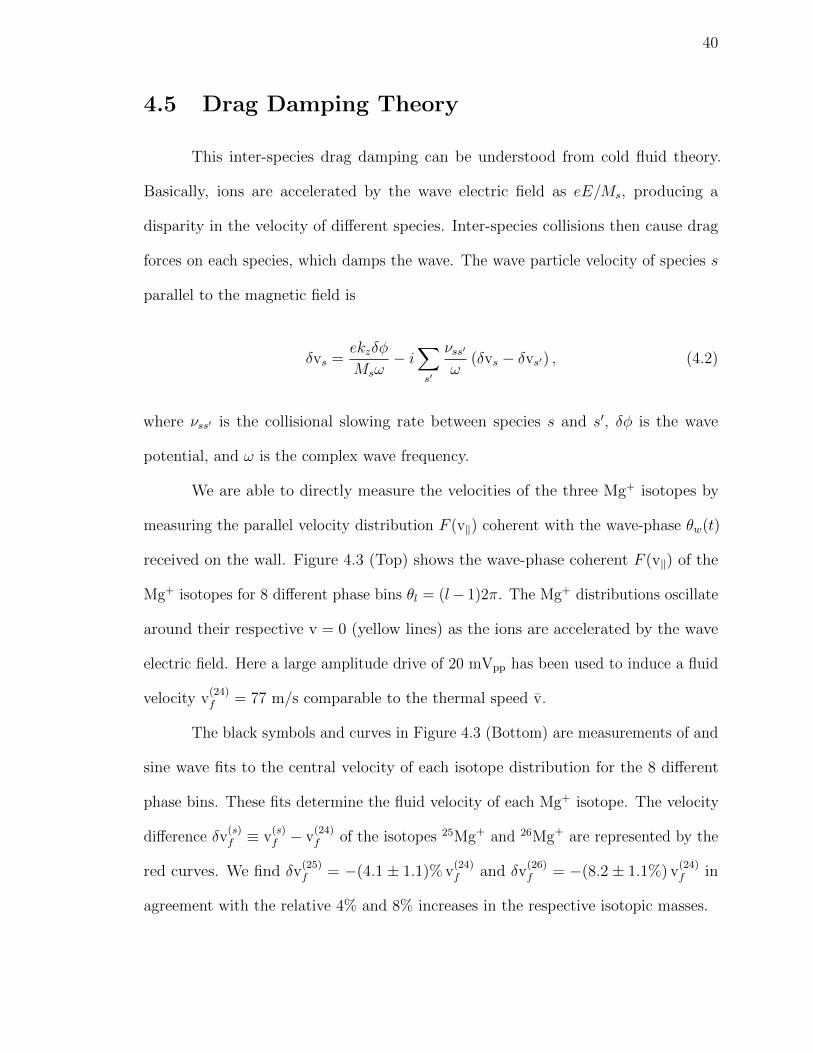
We are able to directly measure the velocities of the three Mg+ isotopes by

measuring the parallel velocity distribution F (v‖) coherent with the wave-phase θw(t)

received on the wall. Figure 4.3 (Top) shows the wave-phase coherent F (v‖) of the

Mg+ isotopes for 8 different phase bins θl = (l− 1)2π. The Mg+ distributions oscillate

around their respective v = 0 (yellow lines) as the ions are accelerated by the wave

electric field. Here a large amplitude drive of 20 mVpp has been used to induce a fluid

velocity v(24)f = 77 m/s comparable to the thermal speed v.

The black symbols and curves in Figure 4.3 (Bottom) are measurements of and

sine wave fits to the central velocity of each isotope distribution for the 8 different

phase bins. These fits determine the fluid velocity of each Mg+ isotope. The velocity

difference δv(s)f ≡ v

(s)f − v

(24)f of the isotopes 25Mg+ and 26Mg+ are represented by the

red curves. We find δv(25)f = −(4.1± 1.1)% v

(24)f and δv

(26)f = −(8.2± 1.1%) v

(24)f in

agreement with the relative 4% and 8% increases in the respective isotopic masses.

41

Detuning([GHz](3.2( 10.4(6.8(

Phase([π(ra

dians](

2(

1(

0(

F(v |

|(,(θ

w)(([cou

nts/(sec(m

W)](

0(

300(

600(

900(

vf( 25 x(δvf(

24Mg+( 25Mg+( 26Mg+(

24Mg+(

25Mg+( 26Mg+(

vf((((=(77(m/s((24)(

θ1$θ2$θ3$θ4$θ5$θ6$θ7$θ8$

WF(8094P8605(

T(≈(8(x(10P4(eV(

(s)(

Figure 4.3: Measurements of the parallel velocity distribution function F (v‖)coherent with the wave-phase θw(t) (Top), each phase is offset for clarity.Black symbols and curves (Bottom) are measurements of and sine wave fits tothe central velocity of the oscillating Mg+ distributions. Red curves (Bottom)are 25× the relative velocity of the Mg+ isotopes to that of 24Mg+.

42

For azimuthally symmetric waves, the drag damping is calculated by solving

for the complex ω = ωr + iγ in the linearized Poisson equation,

1

r

∂

∂r

(r∂δφ

∂r

)− k2zδφ = −4πekz

ω

∑s

n0sδvs (4.3)

using the shooting method. Here, the linearized continuity equation δns = kzn0sδvs/ω

has been used to replace the perturbed density δns with the species velocity δvs.

Also, the equilibrium density n0s has radial dependence at low temperatures when

centrifugal mass separation becomes important. The collisional drag damping rate γ

is proportional to the rate of collisional slowing νss′ .

For plasmas that are both radially uniform and have weak collisionality

(νss′ � ωTG), the collisional drag damping can be solved analytically as

γ ≡ Im(ω) =1

4ω2p

∑s

∑s′

(Ms′ −Ms)2

M2s′

ω2p,sνss′ , (4.4)

where ω2p,s = 4πe2ns/Ms is the species plasma frequency, and ω2

p = Σω2p,s is the total

plasma frequency. This equation is valid in the regime T & 10−3 eV for the plasmas

considered in these experiments. Equation 4.4 recovers the electron-ion drag damping

results of Lenard and Bernstein [56] for neutral plasmas. Here, an enhancement of

νss′ from long-range collisions will increase the drag damping.

4.6 Long-Range Collisionality

Recent theory [12] has shown that two types of long-range collisions occur,

separated by the newly identified diffusion scale length d ≡ b(v2/b2ν2ss′)1/5 ∝ T 1/5,

43

where b = e2/T is the distance of closest approach. The present experiments cover a

range in temperature 10−4 . T . 1 eV, corresponding to a range in the diffusion scale

length 33 . d . 135 µm. For impact parameters ρ < d, collisions occur faster than

the diffusion timescale, so they can be regarded as isolated Boltzmann collisions. In

contrast, for ρ > d, multiple weak collisions occur simultaneously and particles diffuse

in velocity, so Fokker-Planck theory is required. The predicted slowing-down rate has

the “classical” scaling with an enhanced Coulomb logarithm, specifically

νss′ =√πns′ vss′b

2 ln Λ, (4.5)

where

vss′ ≡√

2Tµ/Ms, (4.6)

µ ≡MsMs′/(Ms +Ms′) (4.7)

is the reduced mass, and

ln Λ =4

3ln

(min[rc, λD]

b

)+ p ln

(d

max[b, rc]

)+ 2 ln

(λD

max[d, rc]

)(4.8)

is the enhanced Coulomb logarithm. The first logarithmic term in Eq. 4.8 is from

classical short-range, Boltzmann collisions. The collisional slowing rate is enhanced by

the second and third terms, which represent long-range Boltzmann and Fokker-Planck

collisions respectively. For repulsive (like-sign) collisions p = 5.899; whereas, p = 0 for

attractive (opposite-sign) collisions in neutralized plasmas.

In Fig. 4.4, these short and long-range collision rates are plotted over a range

in temperature for our typical “dirty” plasma. Long-range, 1D Boltzmann collisions

44

102

103

104

105

0

0.5

1

10-4 10-3 10-2

Σνs,

24

Z

T [eV]

Long-Range1D Fokker-Planck

Long-Range1D Boltzmann

Sum

Short-Range3D Boltzmann

ωTG

Z19,24

ν s, 2

4s∑

Figure 4.4: Short and long-range collision rate versus temperature for atypical “dirty” plasma. The dashed purple line is the radial overlap betweenspecies 24Mg+ and H3O

+.

clearly dominate the collisionality in these plasmas, exceeding the classical short-range

collision rate by as much as an order of magnitude. At low temperatures T < 4× 10−4

eV, the plasma becomes strongly magnetized (i.e. rc < b), and the short-range collision

rate approaches zero, because the cyclotron energy of the colliding pairs is an adiabatic

invariant [57]. Long-range, 1D Fokker-Planck collisions are rather weak, and approach

zero for T . 3× 10−4 eV when λD < d.

Predictions of the drag damping theory for both a classical calculation that

assumes only short-range collisions (dashed), and a calculation including the new

long-range enhanced collisional slowing (solid) are shown in Fig. 4.2. Theory is in

quantitative agreement with the experimental results only when long-range collisions

are included, exceeding predictions considering only short-range collisions by as much

as an order of magnitude.

45

The discrepancy between theory and experiments around 10−2 eV may be a

result of another damping mechanism. Cold fluid theory predicts that these TG waves

are also damped from viscous momentum transfer along and across the magnetic

field [58]. In this temperature regime, this damping is too weak (γ ∼ 5 s−1) to explain

the discrepancy we observe, but an enhancement of this damping is predicted from

finite-length effects [59]. Bounce harmonic Landau damping is another mechanism

that may increase the damping in this temperature regime.

4.7 Centrifugal Separation and Fluid Locking

At T . 10−3 eV, the measured and predicted drag damping rates decrease from

the collisional T−3/2 scaling. We analyze two effects that contribute to this decrease.

First, the ions begin to centrifugally separate by mass, with the lighter ions near r = 0.

In Fig. 4.4, the dashed purple curve represents the radial overlap between species

s = 24Mg+ and s′ = H3O+, defined as

Zss′ ≡2∫ Rp0

δs(r)δs′(r)rdr

δsδs′R2p

. (4.9)

On warm plasmas T & 10−3 eV, the species are radially uniform and Zss′ = 1.

However, as the species centrifugally separate, Zss′ decreases, approaching zero for

complete radial separation. This reduction in the radial species overlap decreases

the inter-species drag. Of course, Zss′ represents radially local collisions only, and

non-local interactions will persist even with complete radial separation.

Secondly, the collisionality approaches the wave frequency ωTG around T ∼ 10−3

eV, as shown in Fig. 4.4. For ν ∼ ωTG, the species collide before developing a disparity

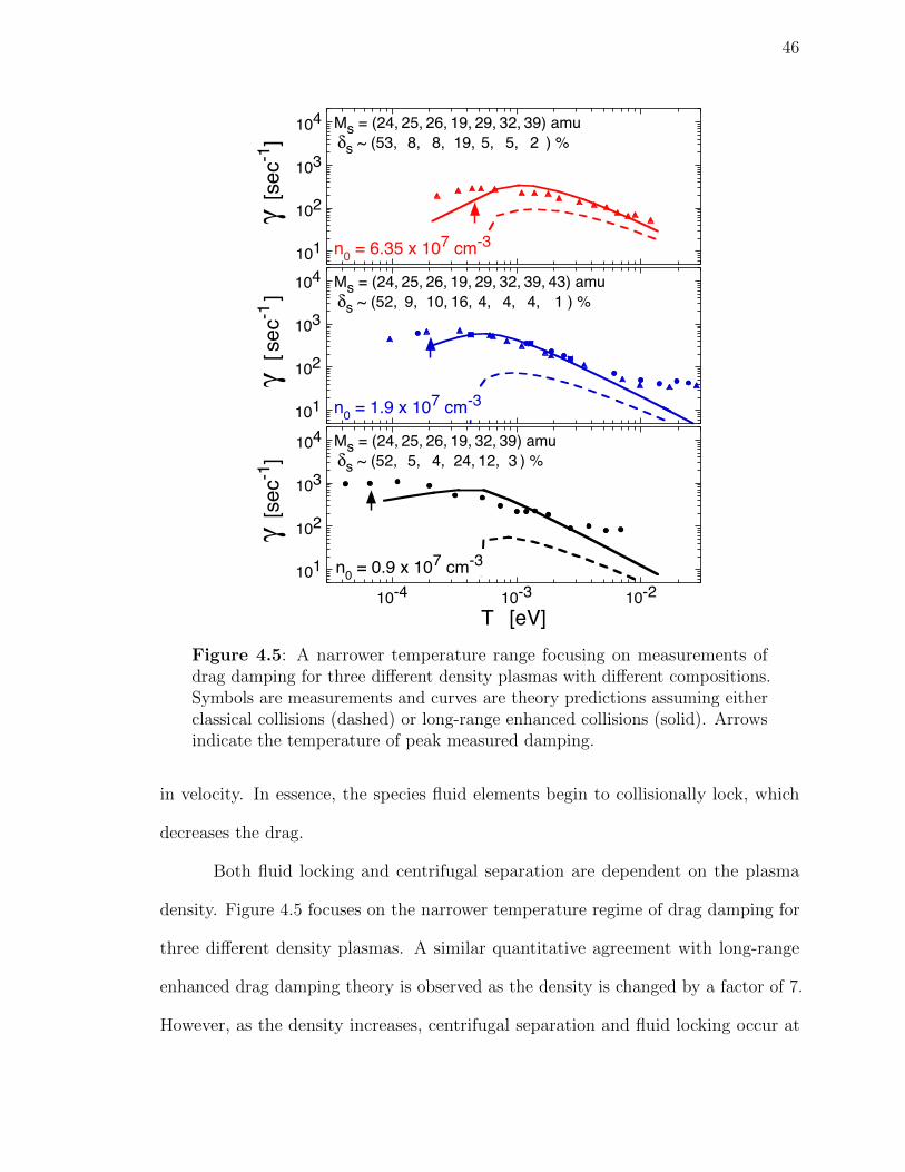
46

101

102

103

104

γ [s

ec-1

]

Ms = (24, 25, 26, 19, 29, 32, 39) amuδs ~ (53, 8, 8, 19, 5, 5, 2 ) %

n0 = 6.35 x 107 cm-3

101

102

103

104γ

[ sec

-1 ]

Ms = (24, 25, 26, 19, 29, 32, 39, 43) amuδs ~ (52, 9, 10, 16, 4, 4, 4, 1 ) %

n0 = 1.9 x 107 cm-3

101

102

103

104

10-4 10-3 10-2

γ [s

ec-1

]

T [eV]

Ms = (24, 25, 26, 19, 32, 39) amuδs ~ (52, 5, 4, 24, 12, 3 ) %

n0 = 0.9 x 107 cm-3

Figure 4.5: A narrower temperature range focusing on measurements ofdrag damping for three different density plasmas with different compositions.Symbols are measurements and curves are theory predictions assuming eitherclassical collisions (dashed) or long-range enhanced collisions (solid). Arrowsindicate the temperature of peak measured damping.

in velocity. In essence, the species fluid elements begin to collisionally lock, which

decreases the drag.

Both fluid locking and centrifugal separation are dependent on the plasma

density. Figure 4.5 focuses on the narrower temperature regime of drag damping for

three different density plasmas. A similar quantitative agreement with long-range

enhanced drag damping theory is observed as the density is changed by a factor of 7.

However, as the density increases, centrifugal separation and fluid locking occur at

47

higher temperatures, and a corresponding increase in the temperature of the measured

“peak” damping is observed. These results suggest that fluid locking and centrifugal

separation are at least in part responsible for the decrease in the damping from the

T−3/2 scaling.

To isolate how reducing the radial overlap between species influences the drag

damping, we use the fact that the plasma thermally equilibrates on a faster timescale

than the species diffuse radially. This enables, for a short period of time, the creation

of a warm plasma with a reduced Zss′ . Figure 4.6 depicts the details of this process.

The plasma is initially cooled to a low temperature T ∼ 10−4 eV, where the species

are centrifugally separated by mass. At r = 0.3 cm on a Rp = 0.5 cm plasma, Fig. 4.6a

shows the measured 25Mg+ and 26Mg+ peaks (blue) as 2× and 4× smaller than

expected for a uniform species distribution. A 500 mVpp, 200 cycle burst at 36 kHz

is applied to the plasma end at 20 ms, heating the plasma. In Fig. 4.6c, the plasma

temperature is shown to re-equilibrate after this heating burst to T ∼ 3× 10−3 eV

on a 20 ms timescale. But, on this timescale, the species have not remixed radially

(Fig. 4.6b). The species generally remix in about 500 ms. By exciting a wave before

the species have remixed (Fig. 4.6d), we are able to measure the drag damping on

a warm plasma with a reduced radial species overlap. This process can be repeated

for different heating burst amplitudes to change the plasma temperature and hence

collisionality, while keeping the species overlap Zss′ roughly constant.

Figure 4.7 shows damping measurements on a standard “dirty” plasma for

which the overlap integral Z19,24(T ) results from centrifugal separation at the abscissa

T; and on the same “dirty” plasma for which the radial species overlap is kept small and

constant at Z19,24 ∼ 0.43 determined by the initial T ∼ 10−4 eV. Clearly, reducing the

48

-20-10

01020

0 20 40 60 80 100 120Wal

l Sig

nal [µV

]

WF 2265WaveDrive

HeatingBurst

time [ms]

d) Digitized Wall Signal

10-4

10-3

10-2

T [e

V]

HeatingBurst

c) Temperature Evolution

WF 2215-2315

0

4

8

12

16

-1 0 1 2 3 4D

etec

ted

Phot

on R

ate

Laser Frequency Detuning [GHz]

[105

/ (se

c m

W)]

T = 9.3 x 10-5 eV

0 - 20 msa)24Mg+

25Mg+ 26Mg+

0

1

2

-1 0 1 2 3 4

T = 2.8 x 10-3 eV

60 - 70 msb)24Mg+

25Mg+ 26Mg+

Figure 4.6: Process for creating a warm plasma with reduced radial overlapbetween the species. The blue curves of (a) and (b) are the measured Mg+

distributions at a radius of 0.3 cm before and after a heating burst; and thered dashed curves are what the distributions would look like on a radiallyuniform plasma. The plasma temperature equilibrates (c) before the specieshave remixed, enabling damping measurements (d) on a warm but radiallynon-uniform plasma.

49

101

102

103

10-4 10-3 10-2

γ [s

ec-1

]

T [eV]

Ms = (24, 25, 26, 19, 29, 32, 39, 43) amuδs ~ (52, 9, 10, 16, 4, 4, 4, 1 ) %

Z T( )

Z 10−4( ) = 0.434x#

Figure 4.7: Measurements of drag damping on a typical “dirty” plasma withcentrifugal separation determined by the abscissa T (blue); and on a plasmawith the same “dirty” composition but with a reduced radial species overlapZ19,24 ∼ 0.43 determined by the initial T ∼ 10−4 eV (red).

species overlap reduces the drag damping. At T ∼ 2× 10−3 eV, Z19,24 differs from 1 to

0.43, and the damping rate is reduced by a factor of 4. The agreement between theory

and experiments for T & 6× 10−4 eV demonstrates that the influence of centrifugal

separation is properly modeled by radially local collisions in this temperature regime.

The data for T < 6× 10−4 eV is inconclusive.

The effect that collisional locking of the species fluid elements has on the

drag damping is investigated by measuring the damping rate of higher frequency,

axial modes. This inter-species drag damping depends on the disparity in the species

velocity, and not on the axial mode structure, so higher frequency axial modes are

predicted to have the same damping rate. However, collisional locking occurs when

the collisionality approaches the wave frequency, so a higher frequency modes will

have less fluid locking.

50

101

102

103

10-4 10-3 10-2

γ [

sec-1

]

T [eV]

Ms = (24, 25, 26, 19, 29, 32, 39, 43) amuδs ~ (48, 9, 10, 20, 4, 4, 4, 1 ) %

mz = 1mz = 2

mz = 3

Figure 4.8: Drag damping measurements on higher frequency, axial modeswith f1 = 27.25 kHz, f2 = 50.35 kHz and f3 = 68.45 kHz. Dashed lines aretheory curves assuming classical collisions and solid curves are that sametheory assuming long-range enhanced collisions.

Figure 4.8 shows the damping rate of the first three axial modes (mz = 1, 2,

and 3). For T & 3 × 10−4 eV, the higher frequency modes are all damped at the

same rate, as predicted by theory in the weak collisionality regime. In contrast, below

T . 3×10−4 eV, the higher frequency modes are more heavily damped, which suggests

less fluid locking. This stronger damping is in qualitative agreement with theory, which

predicts a factor of 2 increase in the damping rate for mz = 3 at T = 3× 10−4 eV.

In general, these TG waves are more heavily damped than the current theory

prediction at ultra-low temperatures T . 4× 10−4 eV. In this centrifugally separated

temperature regime, non-local interaction may be significant, which are not included

in the current theory. Also, for the typical density n0 = 1.9× 107, the plasma ions

becomes moderately correlated, with correlation parameter Γ ≡ e2/aT & 0.2 for

T . 4 × 10−4 eV, where a = (3/4πn0)1/3 is the Wigner-Seitz radius. Correlations

51

may limit the parallel collisionality [60, 61], decreasing the effects of fluid locking and

increasing the predicted damping rates.

4.8 Conclusion

In summary, measurements of collisional inter-species drag damping have pro-

vided the first experimental confirmation of the long-range enhanced, parallel collisional

slowing rate. We presented collisional drag damping theory, which is in quantitative

agreement with the experimental results for a range of plasma compositions and

densities only when long-range collisions are included. At low temperatures T . 10−3

eV, the damping is observed to be reduced from the typical T−3/2 collisional scaling as

centrifugal separation and fluid locking become significant. Non-local interactions and

correlations may be responsible for the discrepancies between theory and experiments

at ultra-low temperatures.

4.9 Acknowledgements

This chapter, in part, is currently being prepared for submission for publication.

M. Affolter, F. Anderegg, D.H.E. Dubin and C.F. Driscoll. The dissertation author was

the primary experimentalist and author of this material. Dubin previously developed

and published the long-range collision theory as Ref. [12].

Chapter 5

Non-Linear Langmuir Waves

5.1 Introduction

This chapter describes experiments and theory on the fundamentals of non-

linear wave couplings, using pure ion plasmas as the model system. This is partially

motivated by non-linear phenomena observed when high power lasers impinge on

plasmas. In these laser-plasma interactions, the high intensity laser couples to ion

acoustic waves (IAWs), causing scattering of the electromagnetic waves. This process,

called stimulated Brillouin scattering (SBS), is a concern for inertial confinement

fusion, as it may reduce the laser energy coupled into the fusion capsule, or reduce

the spherical symmetry. Experiments have shown that SBS saturates at high laser

intensities [62, 63, 64, 65]. Several non-linear effects have been postulated to explain

this saturation, including non-linear frequency shifts [66, 67], and the parametric decay

of the driven IAW into two daughter waves [68, 69, 70, 71, 72]. The near-acoustic

dispersion relation of cold IAWs is similar to the dispersion of Langmuir waves on our

confined ion plasmas, so the fundamental non-linear effects should be similar.

52

53

Here we experimentally quantify non-linear effects in Langmuir waves, including

harmonic generation, non-linear frequency shifts, and the parametric decay instability.

These experiments are conducted on well-controlled, laser-diagnosed, pure ion plasmas

confined in a Penning-Malmberg trap. The plasma waves are azimuthally symmetric

standing waves, discretized by the axial wavenumber kz = mz(π/Lp). The dispersion

ω(k) is basically acoustic, i.e. ω(k) ∝ vphk(1− εk2) with ε ∝ Rp/Lp. By varying the

plasma length, experiments are conducted on plasmas with different deviations from

acoustic dispersion.

At large wave amplitudes, the detected wave density perturbation is no longer

a simple sinusoid. We observe frequency harmonics corresponding to a steepening of

the wave density perturbation, and non-linear frequency shifts of the fundamental.

Both the harmonic content and the relative frequency shifts are more prominent when

the dispersion is more nearly acoustic.

The wave-wave coupling rates are measured between large amplitude mz = 2

waves and small amplitude mz = 1 waves, which have a small frequency detuning

∆ω = 2ω1−ω2. The large wave amplitude is characterized by the parametric coupling

strength Γ0 ≡ (δn2/n0)(ω1+ω2)(R/8), where R ∼ 0.85 is the radial coupling coefficient.

We find that the relative amplitudes of Γ0 and ∆ω are fundamental to the overall

wave-wave interaction. At small excitation amplitudes (2Γ0 < ∆ω), this detuning

causes the mz = 1 mode amplitude to “bounce” at rate ωB ≈ ∆ω with amplitude

excursions ∆A1 ∝ (δn2/n0), in quantitative agreement with three-wave theory [13].

At larger excitation amplitudes (2Γ0 > ∆ω), phase-locked exponential growth of the

mz = 1 mode is observed, consistent with the three-wave instability analysis [13]. Near

the decay threshold 2Γ0 ∼ ∆ω, an unexpected slow average growth of the bouncing

54

mz = 1 wave amplitude is observed, which may be a result of the plasma evolving

during the wave-wave interaction.

5.2 Details of the TG Dispersion Relation

As discussed in Sec. 4.3, the linear dispersion relation of Langmuir waves

in trapped plasmas is near-acoustic, because of the shielding of the confinement

electrodes at Rw. In this section, we investigate the details of this deviation from

acoustic dispersion. The Trivelpiece-Gould (TG) dispersion relation [52, 53] for cold,

azimuthally symmetric, z-periodic travelling waves on a “top-hat” plasma of radius

Rp is approximately

ωmz = ωpkz/k⊥√

1 + (kz/k⊥)2, (5.1)

where kz ≡ mz(π/Lp) and k⊥ = R−1p [2/ ln(Rw/Rp)]1/2 are the axial and transverse

wavenumbers respectively, and ωp =√

4πe2n0/Ms is the plasma frequency. However,

in comparison to experiments, neither kz nor k⊥ are definable to better than 10%. For

our trapped plasmas of length Lp, two counter propagating ±kz traveling waves with

phase velocity vph = ω/kz create a standing wave perturbation. These standing wave

resonances occur when the traveling wave and its reflections from the plasma ends are

in phase.

These waves are excited from a confinement ring located near the plasma end,

and the resulting wave is detected as induced image charge on an off-center ring, as

shown in the Fig. 5.1 inset. Typically, a 40 cycle sine wave burst with an amplitude

AB ∼ 50− 100 mVpp is used. These bursts are ramped to/from full amplitude over

4 cycles to prevent excitation of other waves. By the end of the burst, the plasma

55

has been heated from T ∼ 2 × 10−3 eV to T & 10−2 eV. At this temperature, few

particles are resonant with the wave vph/v ∼ 28 and Landau damping is negligible;

here the waves damp through collisions at a rate γ ∼ 100 /s, as discussed in Sec. 4.4.

Figure 5.1 shows frequency measurements of several small amplitude (AB ∼ 2

mVpp) TG modes for two different plasma lengths. We see that the measured mode

frequencies (symbols) are nearly acoustic (dashed lines), and that the deviation

from acoustic dispersion is dependent on the plasma geometry (k⊥/k1). When the

plasma length is increased from 13.6 cm to 20.3 cm (blue to red data), the relative

deviation from acoustic dispersion ∆ω/ω1 is reduced by about 50%. The on-axis

plasma length is varied over the range 12.4 . Lp . 20.3 cm by varying the strength

of the confining potentials, enabling a corresponding control of the mode frequencies

23.8 & ω1/2π & 13.7 kHz and detuning 3.1 & ∆ω/2π & 0.85 kHz.

The curves in Fig. 5.1 are predictions of Eq. 5.1 with different transverse

wavenumbers. Theory defines k⊥ = R−1p [2/ ln(Rw/Rp)]1/2. This approximation is valid

for plasmas with mzπRw/Lp � 1 and Rp/Rw � 1. We find that for the plasmas in

these experiments with πRw/Lp ∼ 0.6 and Rp/Rw ∼ 0.2 that the measured mz = 1

mode frequency is in agreement with this approximate k⊥ prediction if Lp is increased

by approximately 10% (dotted curves). However, this approximate k⊥ prediction fails

to explain the large deviation from acoustic dispersion of the higher axial modes for

reasonable 10% variations in the plasma parameters (Lp, Rp, and n0).

The discrepancy in the frequency for the higher kz modes is result of k⊥

having a slight kz dependence for these short plasmas, which is ignored in the typical

approximation. The transverse wavenumber k⊥ is determined by the boundary

condition that the radial wave potential be continuous at the plasma radius [52, 53]

56

0

20

40

60

80

0 1 2 3 4 5 6 7

ω / 2

π [k

Hz]

mz

k1 = 0.15 cm-1k1 = 0.23 cm-1

k⊥ / k1 = 9.0

k⊥ / k1 = 14.7

Digi$zer(

+V( +V(

mz(=(1(

mz(=(2(

Figure 5.1: Measured TG dispersion relation (symbols) for two differentplasma geometries compared against cold fluid theory. Dashed lines areacoustic dispersion relations, and dotted/solid curves are TG dispersionrelations with approximate/correct k⊥. The experimentally measured densityn0 and plasma radius Rp are used for the theory predictions with a slightlyincreased plasma length of approximately 1.1Lp. The inset is a sketch of thetypical confinement geometry and the two lowest order modes.

57

given by

k⊥RpJ ′0(k⊥Rp)

J0(k⊥Rp)= kzRp

I ′0(kzRp)K0(kzRw)− I0(kzRw)K ′0(kzRp)

I0(kzRp)K0(kzRw)− I0(kzRw)K0(kzRp)(5.2)

for mθ = 0 modes in a strong magnetic field. For a plasma with Lp = 13.6 cm and

Rp = 0.48 cm, Eq. 5.2 determines k⊥ ≈ 1.96 + 0.12mz. This slight increase of k⊥ for

the higher axial modes increases the deviation from acoustic dispersion in agreement

with the experimental results (solid curves).

5.3 Harmonic Generation

At large wave amplitudes, harmonic generation steepens and increases the peak

wave density perturbation. The detected voltage on the wall of a large amplitude mz

standing mode has the functional form

V (t) ∝∑j

A(j)mz cos(jkzz) cos(jωmz), (5.3)

where j = 1, 2, 3, ... correspond to phase-locked frequency harmonics of the funda-

mental, and A(j)mz = δn

(j)mz/n0 is the amplitude of these harmonics. Experimentally, we

measure V (t) with harmonic content at jωmz . Gauss’s law relates the detected wall

voltage V(j)mz of the cos(jkzz) term to the wave density perturbation δn

(j)mz/n0 as

δn(j)mz

n0

=

(jmzπ

f(j)mzJ0(Rpk⊥)

)(C

qNtot

)V (j)mz , (5.4)

where C is the capacitance of the electrode, f(j)mz ≡ [sin(jkz(z0 + LD)) − sin(jkzz0)],

and z0 is the axial location of the detection electrode of length LD [11]. The accuracy

58

-0.25

0

0.25

0.5

7 7.05 7.1 7.15 7.2t [ms]

WF 99762

j = 1

k⊥ / k1 = 9.0

Σ δn

1 / n0

( j )

j =1 4

Figure 5.2: Detected waveform of a large amplitude mz = 1 TG mode. Theamplitude of the fundamental in shown in red, and the black curve includesthe observe j = 2, 3, and 4 frequency harmonics.

of Eq. 5.4 is dependent on properly determining the plasma n(r, z) equilibrium relative

to the cylindrical detection electrodes, and is typically accurate to within 10% for the

two lowest order modes. Note that to simplify the notation the superscript j = 1 is

typically removed when referring to the fundamental density perturbation.

In Fig. 5.2, the detected temporal waveform of a large amplitude mz = 1 mode

is shown for a typical plasma with k⊥/k1 = 9.0. The wave density perturbation (black

curve) includes frequency harmonics j = 2, 3, and 4. These harmonics lead to a

peak density perturbation about twice the size of the fundamental (red curve). For

this work, we describe the size of these non-linear waves by the amplitude of the

fundamental density perturbation δnmz/n0.

The amplitude of these frequency harmonics (j = 2, 3, and 4) is dependent

on the size of the fundamental density perturbation, and on the deviation from

acoustic dispersion. Figure 5.3 shows that the amplitude of the frequency harmonics

59

10-3

10-2

10-1

0.05 0.07 0.1 0.2 0.3 0.4

δn1 / n

0

δn1 / n0

WF 99762

δn1 / n0 = 1.8(δn1 / n0)2δn1 / n0 = 1.6(δn1 / n0)3δn1 / n0 = 3.4(δn1 / n0)4

j = 2

k⊥ / k1 = 9.0

j = 3

j = 4

(2)

(3)

(4)

( j )

Figure 5.3: Measured amplitude of the frequency harmonics j = 2, 3, and 4of a large amplitude mz = 1 mode. Symbols are the amplitude measurementsand curves are fits to the data.

is proportional to the fundamental density perturbation to the jth power. We also

observe larger harmonic content for more acoustic dispersion relations. When ∆ω/ω1

is reduced by 50% by making the plasma longer, we find roughly a factor of 2 increase

in the j = 2 harmonic A(2)1 .

5.4 Non-Linear Frequency Shifts

Along with this harmonic content, we observe a non-linear frequency shift of the

fundamental. The symbols of Fig. 5.4 are measurements of the non-linear frequency

shift of the mz = 1 mode versus the wave density perturbation squared (δn1/n0)2 for

two different plasma geometries. These frequency shifts are proportional to (δn1/n0)2,

and increase as the plasma dispersion becomes more acoustic (increased k⊥/kz). To

insure that these frequency shifts are measured at roughly the same temperature, the

60

0

1

2

3

0 0.02 0.04 0.06 0.08

δω1 / ω

1 [10

-2]

(δn1 / n0)2

k⊥ / k1 = 9.0

k⊥ / k1 = 14.7

δω1 / ω1 = 35.5 (δn1 / n0)2

δω1 / ω1 = 79.6 (δn1 / n0)2

Figure 5.4: Symbols represent the measured percentage change of the mz = 1mode frequency versus the density perturbation squared for two differentplasma geometries, and dashed lines are fits to the data.

measurements are made shortly after the drive as been turned off before wave damping

heats the plasma. Similar density dependent frequency shifts have been observed in

large amplitude IAW simulations [67, 66].

The observed harmonic content and non-linear frequency shifts are in qualitative

agreement with a cold fluid theory that keeps higher harmonics of the fundamental [14].

This theory predicts similar amplitude scalings of the frequency harmonics, and an

increase in both the harmonic content and the relative frequency shifts as the dispersion

relation becomes more acoustic. However, the predicted magnitude of these effects

are significantly larger than the observations. Presumably, finite-length effects are

important in these experiments, which this periodic theory ignores.

61

5.5 Three-Wave Decay

Large amplitude mz = 2 pump waves are predicted to parametrically couple

to two mz = 1 daughter waves enabling a decay instability. Experiments [71, 72]

and simulations [68, 70] studying IAWs have observed this decay instability, but no

quantitative experiments have been conducted. Cold fluid, three-wave theory predicts

a threshold for the decay related to the deviation from acoustic dispersion by

Γ =

√Γ20 −

(∆ω

2

)2

> 0, (5.5)

where

Γ0 =R

4

(ω1 + ω2

2

)δn2

n0

(5.6)

is the wave-wave coupling strength between the mz = 1 and mz = 2 modes, and

∆ω = 2ω1 − ω2 is the linear frequency detuning. When 2Γ0 > ∆ω, Γ is real and

represents the exponential growth rate ΓE of the mz = 1 mode.

However, when 2Γ0 < ∆ω the coupling strength cannot overcome the detuning.

In this regime, the pump and daughter waves exchange energy in-and-out of phase

resulting in the mz = 1 mode amplitude to “bounce” at a rate ωB = 2ω1 − ω2, where

ω1 is the frequency of the small amplitude daughter wave in the presence of the

pump wave. Three-wave theory considering an infinitesimal daughter wave amplitude

predicts frequency pulling

δω1 ≡ ω1 − ω1 = Im(Γ)−∆ω/2 (5.7)

towards resonance with the pump wave at ω2/2.

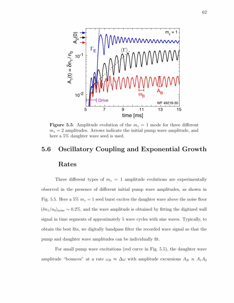
62

10-2

10-1

5 7 9 11 13 15

A 1(t)

= δ

n 1 / n

0

time [ms]

DriveωB

AB

ΓE

WF 49218-30

mz = 1

A 2(0

)

Γ

Figure 5.5: Amplitude evolution of the mz = 1 mode for three differentmz = 2 amplitudes. Arrows indicate the initial pump wave amplitude, andhere a 5% daughter wave seed is used.

5.6 Oscillatory Coupling and Exponential Growth

Rates

Three different types of mz = 1 amplitude evolutions are experimentally

observed in the presence of different initial pump wave amplitudes, as shown in

Fig. 5.5. Here a 5% mz = 1 seed burst excites the daughter wave above the noise floor

(δn1/n0)noise ∼ 0.2%, and the wave amplitude is obtained by fitting the digitized wall

signal in time segments of approximately 5 wave cycles with sine waves. Typically, to

obtain the best fits, we digitally bandpass filter the recorded wave signal so that the

pump and daughter wave amplitudes can be individually fit.

For small pump wave excitations (red curve in Fig. 5.5), the daughter wave

amplitude “bounces” at a rate ωB ≈ ∆ω with amplitude excursions AB ∝ A1A2

63

around an average 〈A1〉. At larger pump wave amplitudes (black curve in Fig. 5.5),

the bounce frequency ωB decreases and the amplitude excursions AB increase. The

amplitude modulation of the daughter wave can be modeled as

A1(t) = 〈A1〉+ AB sin(ωBt). (5.8)

Using this model, we find that the rate of energy exchange between the pump and

daughter waves is

ΓOCR ≡A1(0)

A1(0)=

AB〈A1〉

ωB; (5.9)

identified here as the oscillatory coupling rate (OCR). This OCR provides a measure

of Γ before the exponential growth regime. Figure 5.6 plots this ΓOCR normalized to

∆ω versus the normalized coupling strength for various detunings. We find that ΓOCR

is in quantitative agreement with three-wave theory independent of the deviation from

acoustic dispersion.

As the pump wave amplitude nears the decay threshold (2Γ0/∆ω ∼ 1), a slow

average growth of the “bouncing” mz = 1 wave amplitude is detected, as shown

in Fig. 5.5. This average growth occurs at a rate 〈Γ〉 . 500 s−1 ∼ 0.03∆ω until

δn1/n0 & 2δn2/n0. At the moment, the cause of this average growth is unknown. This

behavior may be a result of the plasma evolving during this wave-wave interaction,

which is not considered in the three-wave analysis. Over the course of this “bouncing”

average growth, the plasma heats as collisions damp the wave. A typical 10% density

perturbation, once damped, results in an ∆T ∼ 5× 10−3 eV increase in the plasma

temperature. Also not considered by three-wave theory is the evolution in the wave

frequencies. We showed in Sec. 5.3 that at these large amplitudes the wave frequencies

64

are shifted away from their linear frequencies, so as the pump and daughter waves

evolve in amplitude ωB changes. At amplitudes near the decay threshold, ωB ∼ 0.5∆ω

and evolves to ∆ω as the waves damp. Recent cold fluid theory that includes frequency

harmonics [14] predicts a similar “bouncing” growth behavior, and connections with

this theory are being pursued.

The dip in the three-wave theory coupling rate at 2Γ0/∆ω = 1 corresponds to

the daughter wave frequency being pulled by δω1 = 0.5∆ω into resonance with the

pump wave. This implies that the rate of energy exchange ωB → 0. Experimentally,

we measure a reduction in the daughter wave frequency δω1 . 0.2∆ω, and no dip

in ΓOCR. A possible cause for this discrepancy is that three-wave theory treats an

infinitesimal daughter wave; whereas, experimentally to measure the mz = 1 frequency

and ΓOCR the wave must be excited above the noise floor to δn1/n0 & 1%.

Exponential growth of the daughter wave is observed for 2Γ0/∆ω & 1 roughly

consistent with three-wave theory. Here no mz = 1 seed is used. The daughter wave

grows above the noise floor, and the rate of this exponential growth is measured by

fitting an exponentially growing sine wave to the digitized wall signal. In general, the

rates ΓE ∼ 3000 − 8000 /s are obtained from fits over 5 − 10 cycles of the growing

mz = 1 wave, and during this growth the mz = 2 amplitude is about 20 times the

mz = 1 amplitude. As shown in Fig. 5.6, this rate of exponential growth scales roughly

as the three-wave theory prediction, but is about 30% lower in magnitude.

It is surprising that three-wave theory is in such good agreement with the ex-

perimental results. This theory ignores the harmonic content and non-linear frequency

shifts of the pump wave, which near the decay threshold are observed to increase

the peak density perturbation by about 20% and decrease the detuning to 0.7∆ω.

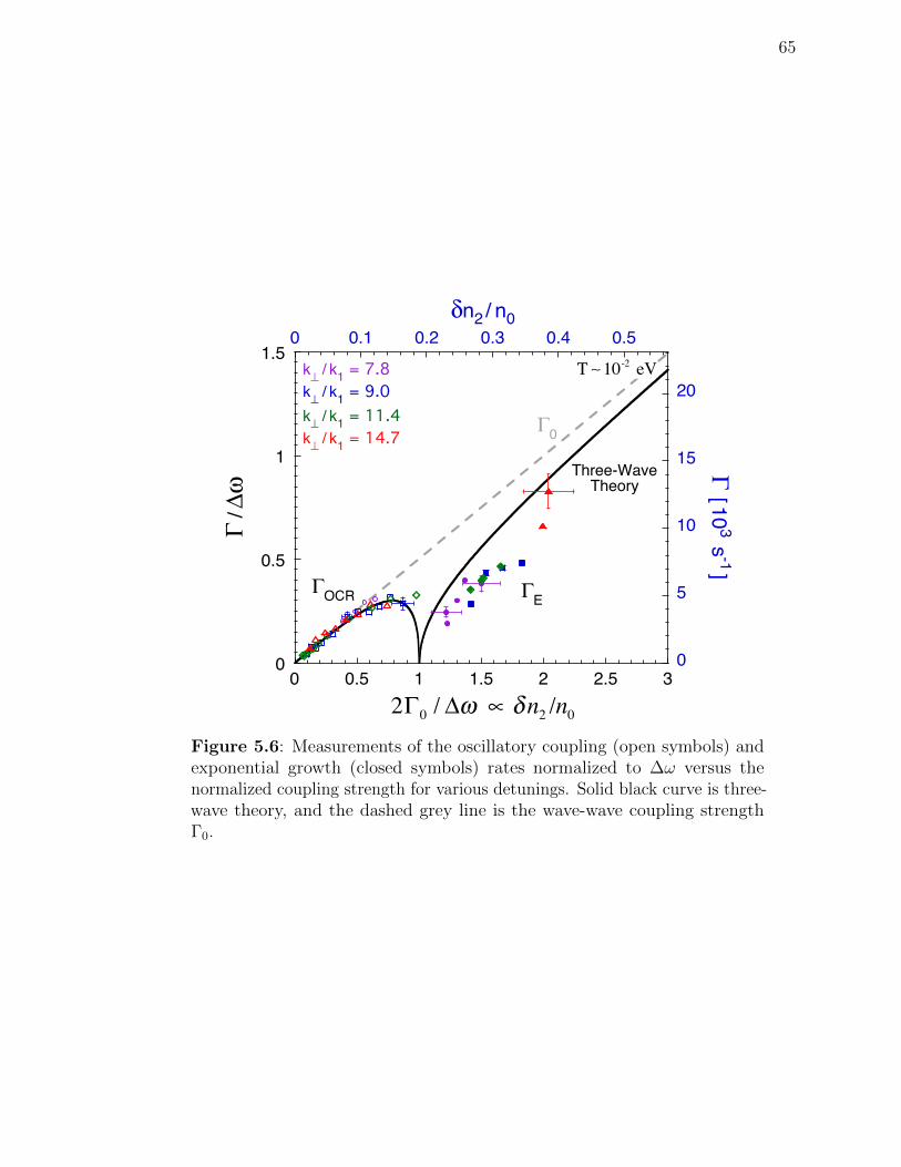
65

0

0.5

1

1.5

0 0.5 1 1.5 2 2.5 3

0 0.1 0.2 0.3 0.4 0.5

0

5

10

15

20

Γ / Δ

ω

2 Γ0 / Δω

Three-WaveTheory

k⊥ / k1 = 7.8k⊥ / k1 = 9.0k⊥ / k1 = 11.4k⊥ / k1 = 14.7 Γ0

ΓOCR ΓE

δn2 / n0

Γ [ 103

s -1 ]

2Γ0 / Δω ∝ δn2 /n0

T 10-2 eV

Figure 5.6: Measurements of the oscillatory coupling (open symbols) andexponential growth (closed symbols) rates normalized to ∆ω versus thenormalized coupling strength for various detunings. Solid black curve is three-wave theory, and the dashed grey line is the wave-wave coupling strengthΓ0.

66

Naively, one would expect that this reduction in the detuning would reduce the decay

threshold to 2Γ0/∆ω ∼ 0.7. In further contradiction, recent cold fluid theory [14] with

strong harmonic content and large non-linear frequency shifts predicts a stabilization

of the decay instability, with decay thresholds 2Γ0/∆ω & 4. That is, the threshold of

this decay is not yet understood.

Figure 5.7 shows RZ-Vlasov simulations for the experimental parameters of the

typical k⊥/k1 = 9.0 plasma. At a temperature T = 0.1 eV, where Landau damping is

negligible, these simulations show oscillatory coupling and exponential growth rates

in agreement with the experimental results. Higher temperature simulations show a

reduction in the instability threshold as kinetic effects become important. For the

highest temperature of T = 0.5 eV, the ratio vph/v = 3 indicates that Landau damping

is strong. Previous experiments investigating the decay instability of higher axial

modes (mz = 4 and 6) on hot electron plasmas [73] observed a decrease in the decay

threshold as the plasma temperature was increased in qualitative agreement with

these Vlasov simulations.

5.7 Conclusion

In summary, large amplitude Langmuir waves with a near-acoustic dispersion

relation are shown to exhibit harmonic generation, non-linear frequency shifts, and a

parametric decay instability. This harmonic content steepens the waveform, and can

increase the peak wave density perturbation by as much as a factor of 2. These large

amplitude waves have non-linear frequency shifts proportional to the wave density

perturbation squared, and dependent on the relative deviation from acoustic dispersion.

Surprisingly, three-wave theory that ignores these effects predicts oscillatory coupling

67

0

0.2

0.4

0.6

0.8

1

0 0.5 1 1.5 2

Γ / Δ

ω

2 Γ0 / Δω

T = 0.5 eV

T = 0.2 eV

T = 0.1 eV

k⊥ / k1 = 9.0

2Γ0 / Δω ∝ δn2 /n0

vph / v 7

vph / v 5

vph / v 3

Figure 5.7: RZ Vlasov simulations of the decay instability for three differ-ent plasma temperatures. Open symbols are oscillatory coupling rates andclosed symbols are exponential growth rates. Arrows indicate the instabilitythreshold.

68

and exponential growth rates in agreement with the experimental results. However,

near the decay threshold an unexpected average “bouncing” growth of the daughter

wave is observed, which is presumably a result of the plasma evolving during the

wave-wave interaction.

5.8 Acknowledgements

This chapter, in part, is currently being prepared for submission for publica-

tion. M. Affolter, F. Anderegg, D.H.E. Dubin, F. Valentini and C.F. Driscoll. The

dissertation author was the primary investigator and author of this material.

Bibliography

[1] D. H. E. Dubin and T. M. ONeil, Reviews of Modern Physics 71, 87 (1999).

[2] J. W. Britton, B. C. Sawyer, A. C. Keith, C.-C. J. Wang, J. K. Freericks, H. Uys,M. J. Biercuk, and J. J. Bollinger, Nature 484, 489 (2012).

[3] R. S. Van Dyck Jr, D. Farnham, and P. Schwinberg, Phys. Rev. Lett. 70, 2888(1993).

[4] R. C. Davidson, Physics of Nonneutral Plasmas, volume 5, Addison-Wesley NewYork, 1990.

[5] F. Anderegg, X.-P. Huang, E. Sarid, and C. F. Driscoll, Review of ScientificInstruments 68, 2367 (1997).

[6] A. G. Marshall, C. L. Hendrickson, and G. S. Jackson, Mass SpectrometryReviews 17, 1 (1998).

[7] E. Sarid, F. Anderegg, and C. F. Driscoll, Physics of Plasmas 2, 2895 (1995).

[8] B. Roth, P. Blythe, H. Wenz, H. Daerr, and S. Schiller, Physical Review A 73,042712 (2006).

[9] B. C. Sawyer, J. G. Bohnet, J. W. Britton, and J. J. Bollinger, Physical ReviewA 91, 011401 (2015).

[10] L.-K. Zhang, D. Rempel, B. N. Pramanik, and M. L. Gross, Mass SpectrometryReviews 24, 286 (2005).

[11] J. R. Danielson, F. Anderegg, and C. F. Driscoll, Phys. Rev. Lett. 92, 245003(2004).

[12] D. H. E. Dubin, Physics of Plasmas 21, 052108 (2014).

[13] A. Ashourvan, Doctoral Dissertation, UCSD (2014).

[14] D. H. E. Dubin and A. Ashourvan, Physics of Plasmas 22, 102102 (2015).

69

70

[15] R. A. MacGill, I. G. Brown, and J. E. Galvin, Review of Scientific Instruments61, 580 (1990).

[16] F. Anderegg, E. M. Hollmann, and C. F. Driscoll, Phys. Rev. Lett. 81, 4875(1998).

[17] T. M. O’Neil, Physics of Fluids 24, 1447 (1981).

[18] D. Larson, J. Bergquist, J. Bollinger, W. M. Itano, and D. Wineland, Phys. Rev.Lett. 57, 70 (1986).

[19] G. Andresen et al., Phys. Rev. Lett. 106, 145001 (2011).

[20] D. H. E. Dubin, 1521, 26 (2013).

[21] J. Adam, Plasma Physics and Controlled Fusion 29, 443 (1987).

[22] R. Gilgenbach, M. Read, K. Hackett, R. Lucey, B. Hui, V. Granatstein, K. Chu,A. England, C. Loring, O. Eldridge, H. Howe, A. Kulchar, E. Lazarus, M. Mu-rakami, and J. Wilgen, Phys. Rev. Lett. 44, 647 (1980).

[23] H. Laqua, V. Erckmann, H. Hartfuß, H. Laqua, and W7-AS ECRH Group, Phys.Rev. Lett. 78, 3467 (1997).

[24] F. Volpe, H. Laqua, and W7-AS Team, Review of Scientific Instruments 74, 1409(2003).

[25] G. Taylor, P. Efthimion, B. Jones, T. Munsat, J. Spaleta, J. Hosea, R. Kaita,R. Majeski, and J. Menard, Review of Scientific Instruments 72, 285 (2001).

[26] M. Easterling, T. Mize, and I. Amster, Analytical Chemistry 71, 624 (1999).

[27] C. Masselon, A. Tolmachev, G. Anderson, R. Harkewicz, and R. Smith, Journalof the American Society for Mass Spectrometry 13, 99 (2002).

[28] R. Wong and I. Amster, International Journal of Mass Spectrometry 265, 99(2007).

[29] E. B. Ledford, D. L. Rempel, and M. L. Gross, Analytical Chemistry 56, 2744(1984).

[30] R. W. Gould, Physics of Plasmas 2, 1404 (1995).

[31] D. H. E. Dubin, Physics of Plasmas 20, 042120 (2013).

[32] R. W. Gould and M. A. LaPointe, Phys. Rev. Lett. 67, 3685 (1991).

[33] S. Barlow, J. Luine, and G. Dunn, International Journal of Mass Spectrometryand Ion Processes 74, 97 (1986).

71

[34] D. Rempel, E. Ledford Jr, S. Huang, and M. Gross, Analytical Chemistry 59,2527 (1987).

[35] A. Peurrung, R. Kouzes, and S. Barlow, International Journal of Mass Spectrom-etry and Ion Processes 157, 39 (1996).

[36] K. S. Fine and C. F. Driscoll, Physics of Plasmas 5, 601 (1998).

[37] J. Jeffries, S. Barlow, and G. Dunn, International Journal of Mass Spectrometryand Ion Processes 54, 169 (1983).

[38] R. Burton, K. Matuszak, C. Watson, and J. Eyler, Journal of the AmericanSociety for Mass Spectrometry 10, 1291 (1999).

[39] D. H. E. Dubin, Phys. Rev. Lett. 79, 2678 (1997).

[40] F. Anderegg, X.-P. Huang, C. F. Driscoll, E. M. Hollmann, T. M. O’Neil, andD. H. E. Dubin, Phys. Rev. Lett. 78, 2128 (1997).

[41] D. H. E. Dubin and T. M. O’Neil, Phys. Rev. Lett. 78, 3868 (1997).

[42] E. M. Hollmann, F. Anderegg, and C. F. Driscoll, Phys. Rev. Lett. 82, 4839(1999).

[43] C. F. Driscoll, J. H. Malmberg, and K. S. Fine, Phys. Rev. Lett. 60, 1290 (1988).

[44] J. M. Kriesel and C. F. Driscoll, Phys. Rev. Lett. 87, 135003 (2001).

[45] G. Andresen et al., Nature 468, 673 (2010).

[46] G. Gabrielse, X. Fei, L. A. Orozco, R. L. Tjoelker, J. Haas, H. Kalinowsky, T. A.Trainor, and W. Kells, Phys. Rev. Lett. 63, 1360 (1989).

[47] B. M. Jelenkovic, A. S. Newbury, J. J. Bollinger, W. M. Itano, and T. B. Mitchell,Phys. Rev. A 67, 063406 (2003).

[48] A. M. Beloborodov and C. Thompson, The Astrophysical Journal 657, 967(2007).

[49] J. A. Boedo, D. L. Rudakov, R. A. Moyer, G. R. McKee, R. J. Colchin, M. J.Schaffer, P. Stangeby, W. West, S. L. Allen, T. E. Evans, et al., Physics ofPlasmas 10, 1670 (2003).

[50] Y. Liang, H. Koslowski, P. Thomas, E. Nardon, B. Alper, P. Andrew, Y. Andrew,G. Arnoux, Y. Baranov, M. Becoulet, et al., Phys. Rev. Lett. 98, 265004 (2007).

[51] B. LaBombard, J. Rice, A. Hubbard, J. Hughes, M. Greenwald, J. Irby, Y. Lin,B. Lipschultz, E. Marmar, C. Pitcher, et al., Nuclear Fusion 44, 1047 (2004).

72

[52] A. Trivelpiece and R. Gould, Journal of Applied Physics 30, 1784 (1959).

[53] J. R. Danielson, D. H. E. Dubin, R. G. Greaves, and C. M. Surko, Reviews ofModern Physics 87, 247 (2015).

[54] F. Anderegg, M. Affolter, A. A. Kabantsev, D. H. E. Dubin, A. Ashourvan, andC. F. Driscoll, Physics of Plasmas 23, 055706 (2016).

[55] A. Ashourvan and D. H. E. Dubin, Physics of Plasmas 21, 052109 (2014).

[56] A. Lenard and I. B. Bernstein, Physical Review 112, 1456 (1958).

[57] M. E. Glinsky, T. M. ONeil, M. N. Rosenbluth, K. Tsuruta, and S. Ichimaru,Physics of Fluids B 4, 1156 (1992).

[58] M. Anderson and T. ONeil, Physics of Plasmas 14, 112110 (2007).

[59] M. W. Anderson, T. M. ONeil, D. H. E. Dubin, and R. W. Gould, Physics ofPlasmas 18, 102113 (2011).

[60] G. Dimonte and J. Daligault, Phys. Rev. Lett. 101, 135001 (2008).

[61] S. D. Baalrud and J. Daligault, Phys. Rev. Lett. 110, 235001 (2013).

[62] A. Ng, L. Pitt, D. Salzmann, and A. A. Offenberger, Phys. Rev. Lett. 42, 307(1979).

[63] J. E. Bernard and J. Meyer, Phys. Rev. Lett. 55, 79 (1985).

[64] S. H. Glenzer, L. M. Divol, R. L. Berger, C. Geddes, R. K. Kirkwood, J. D.Moody, E. A. Williams, and P. E. Young, Phys. Rev. Lett. 86, 2565 (2001).

[65] C. E. Clayton, C. Joshi, and F. F. Chen, Phys. Rev. Lett. 51, 1656 (1983).

[66] T. Chapman, R. Berger, S. Brunner, and E. Williams, Phys. Rev. Lett. 110,195004 (2013).

[67] R. Berger, S. Brunner, T. Chapman, L. Divol, C. Still, and E. Valeo, Physics ofPlasmas 20, 032107 (2013).

[68] T. Chapman, S. Brunner, J. Banks, R. Berger, B. Cohen, and E. Williams,Physics of Plasmas 21, 042107 (2014).

[69] D. Pesme, C. Riconda, and V. Tikhonchuk, Physics of Plasmas 12, 092101 (2005).

[70] B. Cohen, E. Williams, R. Berger, D. Pesme, and C. Riconda, Physics of Plasmas16, 032701 (2009).

[71] H. Bandulet, C. Labaune, K. Lewis, and S. Depierreux, Phys. Rev. Lett. 93,035002 (2004).

73

[72] C. Niemann, S. H. Glenzer, J. Knight, L. Divol, E. A. Williams, G. Gregori, B. I.Cohen, C. Constantin, D. H. Froula, D. S. Montgomery, and R. P. Johnson, Phys.Rev. Lett. 93, 045004 (2004).

[73] H. Higaki, Plasma Physics and Controlled Fusion 39, 1793 (1997).